Embed Size (px)
Citation preview
Multi-Edge Low-Density Parity-Check Coded Modulation
by
Lei Zhang
A thesis submitted in conformity with the requirementsfor the degree of Master of Applied Science
Graduate Department of Edward Rogers Sr. Department of Electricaland Computer Engineering
University of Toronto
Copyright c© 2011 by Lei Zhang
Abstract
Multi-Edge Low-Density Parity-Check Coded Modulation
Lei Zhang
Master of Applied Science
Graduate Department of Edward Rogers Sr. Department of Electrical and Computer
Engineering
University of Toronto
2011
A method for designing low-density parity-check (LDPC) codes for bandwidth-efficient
high-order coded modulation is proposed. Code structure utilizes the multi-edge-type
LDPC code ensemble to achieve an improved match between codeword bit protection ca-
pabilities and modulation bit-channel capacities over existing LDPC coded modulation
techniques. The multi-dimensional EXIT vector field for the specific multi-edge parame-
terization is developed for the analysis and design of code ensembles. A multi-dimensional
EXIT decoding convergence condition is derived to enable efficient optimization. Code
design results in terms of ensemble thresholds and finite-length Monte-Carlo simulations
indicate that the new technique improves on the state-of-the-art performance, with sig-
nificantly lower design and implementation complexity.
ii

Acknowledgements
This thesis would not have been written but for the great number of people from
whom I have received sage advice, unparalleled friendship and unconditional love. At the
forefront of this amazing group is my advisor, professor Frank Kschischang, whose over-
arching perspective, originality of ideas, seemingly boundless knowledge and meticulous
attention to detail have ensured a smooth and thoroughly enjoyable research experience
for me. In the last few years I’ve experienced tremendous academic and professional
growth under his guidance, inspired by his dedication and excellence in all aspects of an
academic career, from research, teaching, to professional commitments. It has been an
honour and a pleasure to work with professor Kschischang.
A special thank you to Dr. Benjamin Smith, whose wealth of knowledge, insights
and advice have greatly facilitated my research. I’ve also enjoyed the many stimulating
conversations we’ve had regarding careers and the minutiae of academia. It is one of
the many aspects which allowed him to become a valuable role model to an incipient
researcher such as myself.
To all my friends, I honestly believe that without your encouragement, company, and
coffee breaks, I would not have been able to overcome several particularly trying stages
throughout this endeavour. Thank you all. I hope to have the opportunity to repay each
and every one of you in kind.
Finally, to my parents, I dedicate this thesis to you as a small token of my appreciation
for your unconditional love and support. I love you both from the bottom of my heart.
iii
Contents
1 Introduction 1
1.1 Improving BICM-LDPC . . . . . . . . . . . . . . . . . . . . . . . . . . . 5
1.2 Literature Review . . . . . . . . . . . . . . . . . . . . . . . . . . . . . . . 8
1.3 Thesis Outline . . . . . . . . . . . . . . . . . . . . . . . . . . . . . . . . . 10
2 Technical Background 11
2.1 Target System . . . . . . . . . . . . . . . . . . . . . . . . . . . . . . . . . 11
2.1.1 IID channel adapter . . . . . . . . . . . . . . . . . . . . . . . . . 13
2.1.2 Non-iterative vs. Iterative demapping . . . . . . . . . . . . . . . . 14
2.1.3 Shaping . . . . . . . . . . . . . . . . . . . . . . . . . . . . . . . . 16
2.2 Analysis and Design of Binary LDPC Codes . . . . . . . . . . . . . . . . 16
2.2.1 Ensemble-based design and density evolution . . . . . . . . . . . . 16
2.2.2 Extrinsic information transfer charts . . . . . . . . . . . . . . . . 23
2.3 Multi-edge-type LDPC Codes . . . . . . . . . . . . . . . . . . . . . . . . 26
3 Multi-edge LDPC Coded Modulation 31
3.1 Multi-edge Parameterization . . . . . . . . . . . . . . . . . . . . . . . . . 31
3.1.1 Check degree edge-type assignment . . . . . . . . . . . . . . . . . 35
3.2 Multi-edge Optimization . . . . . . . . . . . . . . . . . . . . . . . . . . . 38
3.2.1 Multi-dimensional EXIT vector field . . . . . . . . . . . . . . . . 39
3.2.2 Design of multi-edge coded modulation . . . . . . . . . . . . . . . 47
iv
4 Results 61
4.1 Threshold . . . . . . . . . . . . . . . . . . . . . . . . . . . . . . . . . . . 61
4.1.1 Discussion . . . . . . . . . . . . . . . . . . . . . . . . . . . . . . . 62
4.1.2 High code rate designs . . . . . . . . . . . . . . . . . . . . . . . . 65
4.2 Finite-length . . . . . . . . . . . . . . . . . . . . . . . . . . . . . . . . . . 65
4.2.1 Rate 3/4 Gray-labelled 16-QAM . . . . . . . . . . . . . . . . . . . 68
4.2.2 Rate 1/2 Gray-labelled 16-QAM . . . . . . . . . . . . . . . . . . . 72
4.2.3 Fixed BER performance comparison . . . . . . . . . . . . . . . . 72
5 Conclusion 76
Bibliography 78
v
List of Tables
3.1 Density evolution thresholds for the (3,6) regular LDPC check degree edge-
type split pairings under Gray-labelled 16-QAM. . . . . . . . . . . . . . . 36
3.2 Density evolution thresholds for the (3,9) regular LDPC check degree edge-
type split pairings under Gray-labelled 16-QAM. . . . . . . . . . . . . . . 37
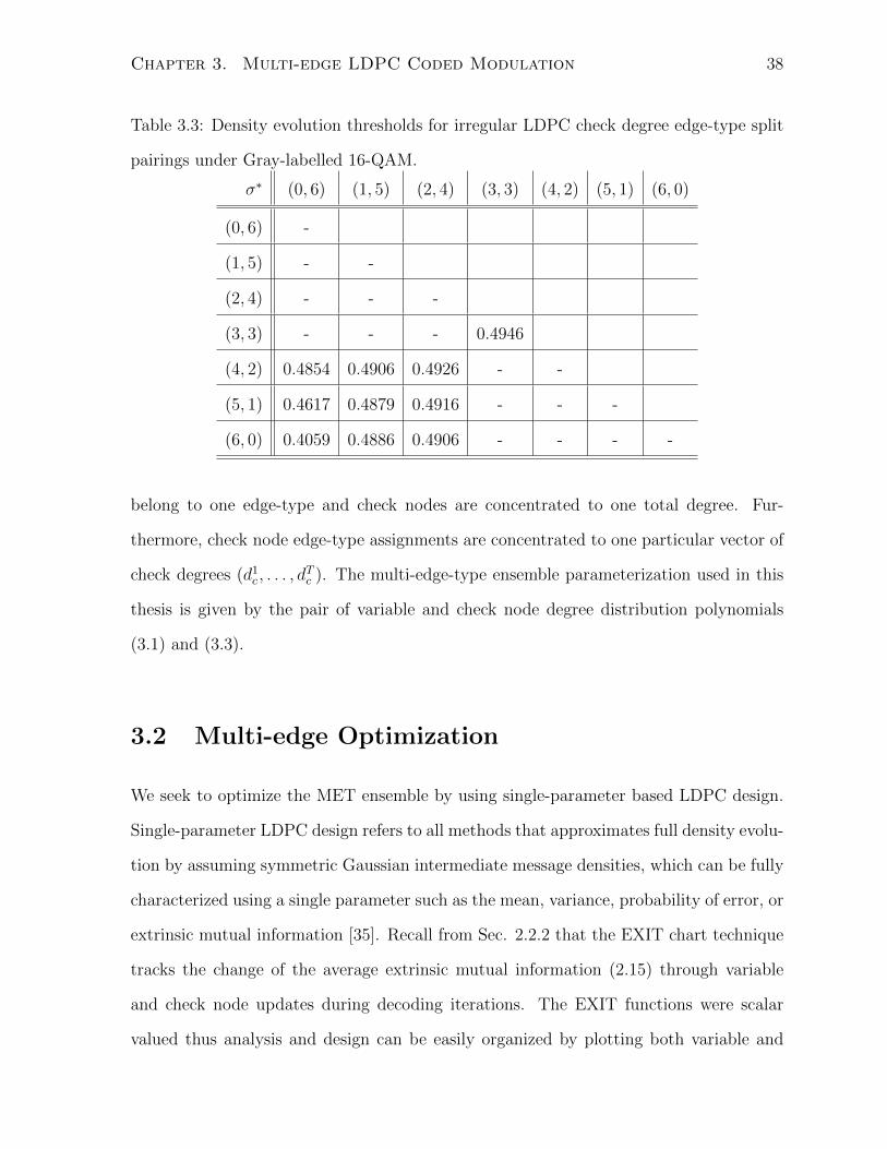
3.3 Density evolution thresholds for irregular LDPC check degree edge-type
split pairings under Gray-labelled 16-QAM. . . . . . . . . . . . . . . . . 38
3.4 Bit-channel capacities for Gray-labelled 2n-QAM at rate (n− 1)/n . . . . 59
4.1 ME-LCM-OPT optimized ensembles for 2n-QAM rate (n− 1)/n codes . 63
4.2 ME-LCM-OPT optimized ensembles of various code rates for 16-QAM . 66
4.3 ME-LCM-OPT optimized ensembles of various code rates for 16-QAM
(continued) . . . . . . . . . . . . . . . . . . . . . . . . . . . . . . . . . . 67
4.4 Legend for data points in Fig. 4.6 . . . . . . . . . . . . . . . . . . . . . . 75
vi
List of Figures
1.1 Decoding block diagrams of BICM and MLC-MSD with 4 bit-levels. . . . 4
1.2 Tanner graph for parity check matrix in Eqn. 1.3. . . . . . . . . . . . . . 5
1.3 Gray-labelled 16-QAM constellation with labels corresponding to bits b0b1b2b3. 7
1.4 Histogram of LLRs for Gray-mapped 16-QAM bit-levels b0, b1, b2, b3. . . 7
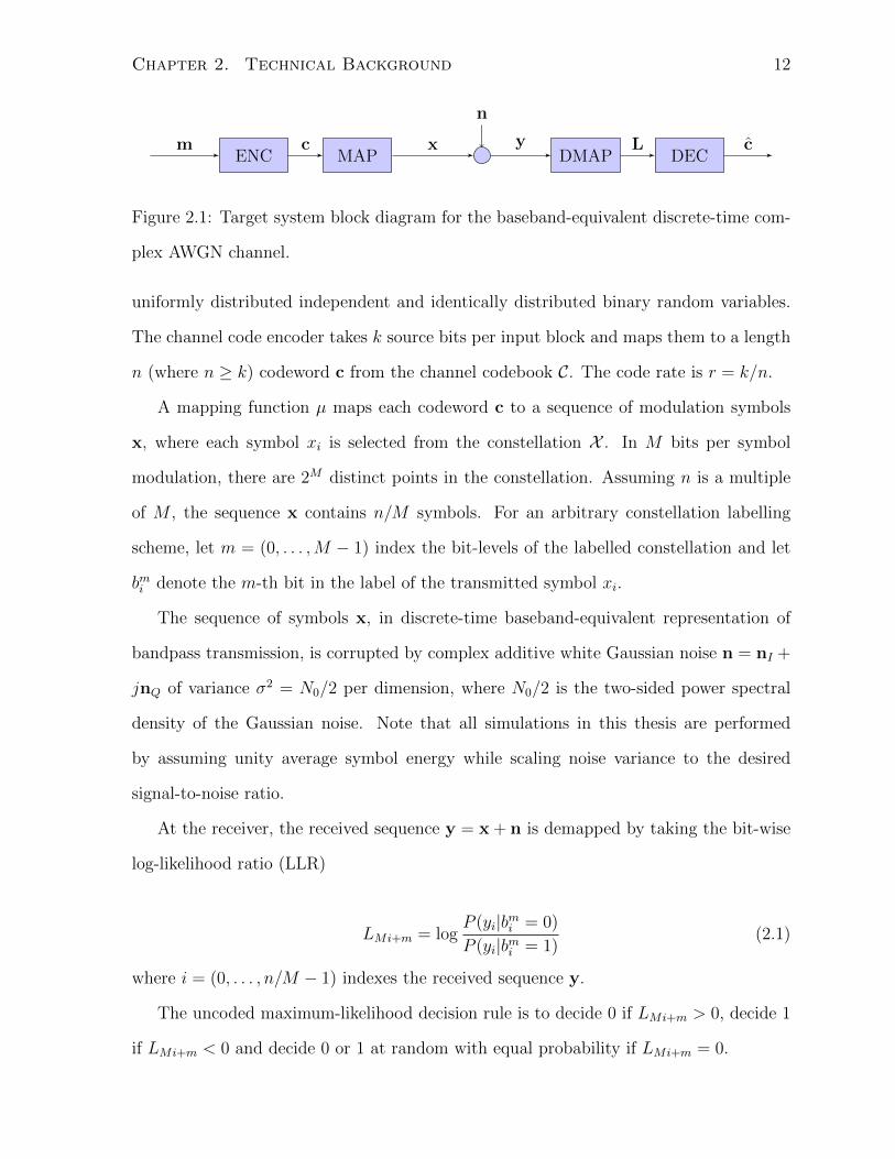
2.1 Target system block diagram for the baseband-equivalent discrete-time
complex AWGN channel. . . . . . . . . . . . . . . . . . . . . . . . . . . . 12
2.2 Bit-channel and symbol-channel capacities of 16-QAM for set-partition
labelled MLC/MSD and Gray-labelled BICM. . . . . . . . . . . . . . . . 15
2.3 EXIT chart of optimized rate = 0.33 ensemble at threshold of -1.91 dB
Es/N0. . . . . . . . . . . . . . . . . . . . . . . . . . . . . . . . . . . . . . 25
2.4 A possible multi-edge-type representation of the Tanner graph in Fig. 1.2 27
3.1 Tanner graph of the 2 edge-type specified MET parameterization, node
degrees are illustrative and not meant to be realistic. . . . . . . . . . . . 33
3.2 Multi-dimensional EXIT vector field for 2 edge-types at threshold σ∗ =
0.3665. . . . . . . . . . . . . . . . . . . . . . . . . . . . . . . . . . . . . . 44
3.3 Multi-dimensional EXIT vector field for 2 edge-types at above threshold
σ = 0.3666. . . . . . . . . . . . . . . . . . . . . . . . . . . . . . . . . . . 46
3.4 Backward-difference vector field of 2 edge-types at threshold σ∗ = 0.3665. 51
vii
3.5 Backward-difference vector field of 2 edge-types at above threshold σ =
0.3666. . . . . . . . . . . . . . . . . . . . . . . . . . . . . . . . . . . . . . 55
4.1 ME-LCM-OPT optimized ensembles for 2n-QAM rate (n− 1)/n codes. . 64
4.2 Probability of bit and errors for n = 4096 rate 3/4 code and Gray-labelled
16-QAM. . . . . . . . . . . . . . . . . . . . . . . . . . . . . . . . . . . . . 69
4.3 Probability of bit and errors for n = 8192 rate 3/4 code and Gray-labelled
16-QAM. . . . . . . . . . . . . . . . . . . . . . . . . . . . . . . . . . . . . 70
4.4 Probability of bit and errors for n = 16384 rate 3/4 code and Gray-labelled
16-QAM. . . . . . . . . . . . . . . . . . . . . . . . . . . . . . . . . . . . . 71
4.5 Probability of bit and errors for n = 16200 rate 1/2 code and Gray-labelled
16-QAM. . . . . . . . . . . . . . . . . . . . . . . . . . . . . . . . . . . . . 73
4.6 Comparison of Es/N0 required to achieve BER of 10−5 at different spectral
efficiencies for Gray-labelled 16-QAM. . . . . . . . . . . . . . . . . . . . . 74
viii
Chapter 1
Introduction
In many communication systems, the modulation and channel code are designed sepa-
rately. Several factors motivate this paradigm. A complicated modulation system can
often be encapsulated by a simple channel model, such as the binary symmetric channel
(BSC), to greatly simplify the channel code design without incurring a significant loss in
performance. For applications with high error tolerance, the uncoded modulation error
rate may be sufficiently low to obviate the need for a channel code. Even the pedagogical
tradition in undergraduate and graduate digital communication courses dictates sepa-
rating modulation and coding. The most dominant reason, however, is the complexity
of designing the modulation and channel code in conjunction. The trade-off between
the cost to design the more complex system and the performance gains from doing so
often results in the pragmatic engineering solution of the distinct modulation-coding
architecture.
For applications where bandwidth is a limiting resource, the gain in combining mod-
ulation and channel coding significantly outweighs the increase in system complexity. A
well-known example of coded modulation is Trellis Coded Modulation (TCM) [1]. TCM
combines the Euclidean distance properties of the modulation signal constellation with
the Hamming distance properties of the error-correcting convolutional (trellis) code in its
1
Chapter 1. Introduction 2
design process. Design rules map trellis transitions of the convolutional code to subsets
of the constellation of different Euclidean distances. In the early 1980’s, telephone line
modem designers considered 9600 kbit/s to be the limiting throughput under standard
bandwidth and power constraints. With the introduction of TCM in 1984, telephone
modems achieved 14.4 kbit/s and higher [2], which helped usher in the meteoric rise of
personal dial-up Internet services.
After the discovery of capacity-approaching turbo and low-density parity-check (LDPC)
codes in the early 90’s [3,4], coded modulation using these modern codes evolved follow-
ing two dominant approaches based on modulation bit-level capacities. Bit-Interleaved
Coded-Modulation (BICM) [5] uses an interleaver between the channel code encoder and
the bit-to-symbol mapper. BICM averages the Euclidean distances of different modula-
tion bit-levels so that the underlying error-correcting code experiences an average noise
degradation from the channel. The BICM bit-channel capacities, I(bi;Y ), can be shown
to be an approximation of the expanded symbol channel mutual information using the
“chain rule”
I(X;Y ) = I(b0, . . . , bn−1;Y )
=n−1∑i=0
I(bi;Y |b0, . . . , bi−1) (1.1)
≥n−1∑i=0
I(bi;Y ). (1.2)
Even though capacity is lost in the process, it has been shown in [5] that BICM
with Gray labelling can closely approximate the finite-constellation constrained channel
capacity. A capacity-approaching code can then be designed for each bit-channel capacity.
An alternative method of coded modulation is Multi-Level Coding (MLC) [6, 7]. In
MLC, for a fixed constellation label, the bit-level capacities are given by (1.1) and achieves
the symbol channel capacity. Again, capacity-approaching codes can be designed for each
bit-channel. At the receiver, decoding progresses in a level-by-level fashion called Multi-
Chapter 1. Introduction 3
Stage Decoding (MSD) [7]. Initially only the decoder for bit-level b0 is active. Assuming
all b0 bits are correctly decoded, the receiver uses this side-information along with received
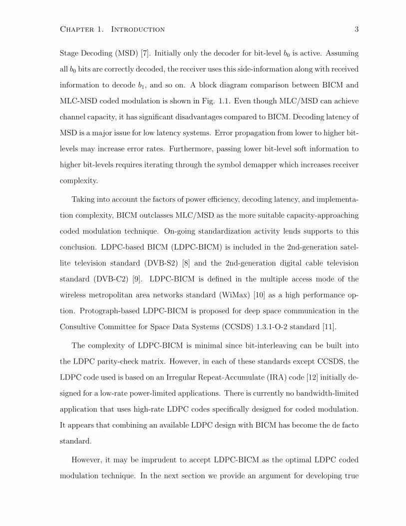
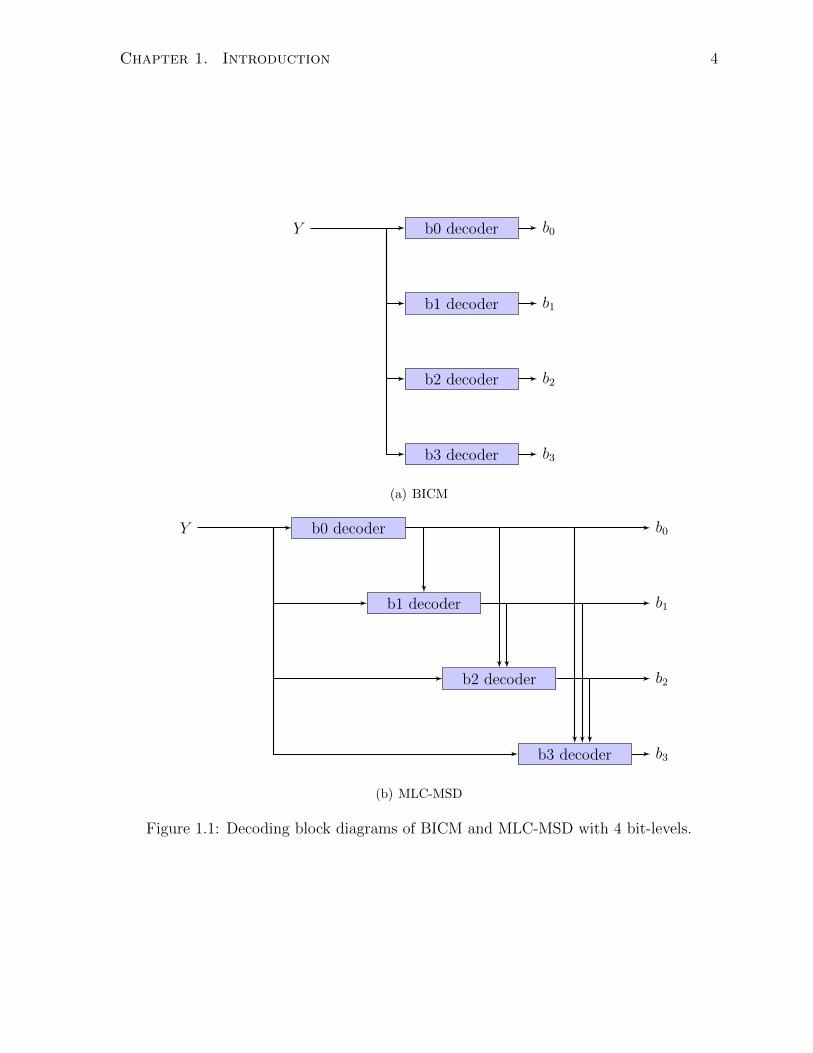
information to decode b1, and so on. A block diagram comparison between BICM and
MLC-MSD coded modulation is shown in Fig. 1.1. Even though MLC/MSD can achieve
channel capacity, it has significant disadvantages compared to BICM. Decoding latency of
MSD is a major issue for low latency systems. Error propagation from lower to higher bit-
levels may increase error rates. Furthermore, passing lower bit-level soft information to
higher bit-levels requires iterating through the symbol demapper which increases receiver
complexity.
Taking into account the factors of power efficiency, decoding latency, and implementa-
tion complexity, BICM outclasses MLC/MSD as the more suitable capacity-approaching
coded modulation technique. On-going standardization activity lends supports to this
conclusion. LDPC-based BICM (LDPC-BICM) is included in the 2nd-generation satel-
lite television standard (DVB-S2) [8] and the 2nd-generation digital cable television
standard (DVB-C2) [9]. LDPC-BICM is defined in the multiple access mode of the
wireless metropolitan area networks standard (WiMax) [10] as a high performance op-
tion. Protograph-based LDPC-BICM is proposed for deep space communication in the
Consultive Committee for Space Data Systems (CCSDS) 1.3.1-O-2 standard [11].
The complexity of LDPC-BICM is minimal since bit-interleaving can be built into
the LDPC parity-check matrix. However, in each of these standards except CCSDS, the
LDPC code used is based on an Irregular Repeat-Accumulate (IRA) code [12] initially de-
signed for a low-rate power-limited applications. There is currently no bandwidth-limited
application that uses high-rate LDPC codes specifically designed for coded modulation.
It appears that combining an available LDPC design with BICM has become the de facto
standard.
However, it may be imprudent to accept LDPC-BICM as the optimal LDPC coded
modulation technique. In the next section we provide an argument for developing true
Chapter 1. Introduction 4
Y b0 decoder
b1 decoder
b2 decoder
b3 decoder
b0
b1
b2
b3
(a) BICM
Y b0 decoder
b1 decoder
b2 decoder
b3 decoder
b0
b1
b2
b3
(b) MLC-MSD
Figure 1.1: Decoding block diagrams of BICM and MLC-MSD with 4 bit-levels.
Chapter 1. Introduction 5
LDPC coded modulation that accounts for modulation bit-level differences in LDPC
code design. Significant performance gains maybe achievable with such an improvement
to LDPC-BICM.
1.1 Improving BICM-LDPC
To introduce the argument for an improved BICM-LDPC design technique, we introduce
a few necessary details of LDPC codes. To keep the treatment brief, we relegate additional
technical details to Ch. 2.
LDPC codes are linear codes with sparse parity-check matrices. Each column of the
LDPC parity-check matrix represents a codeword bit. The non-zero entries in a column
denote the parity-check equations to which the particular codeword bit belongs. The
non-zero entries in a row of the parity-check matrix denote the codeword bits checked
by that parity-check equation. The parity-check matrix can be visually represented by
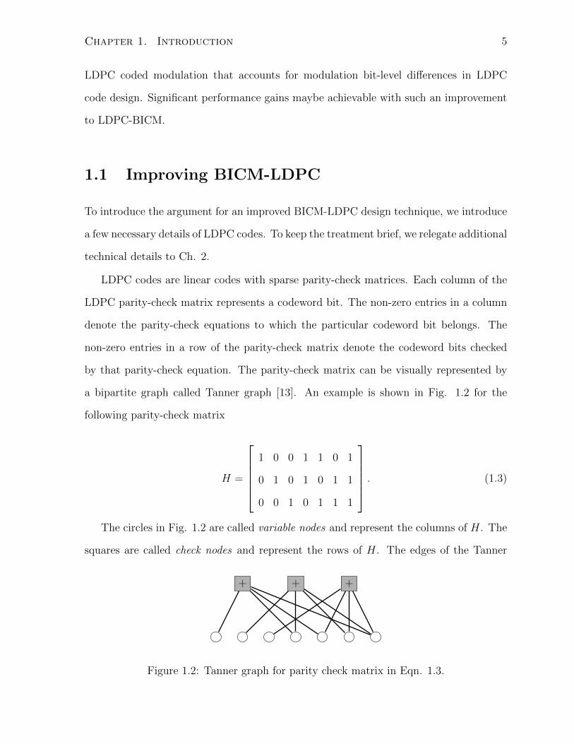
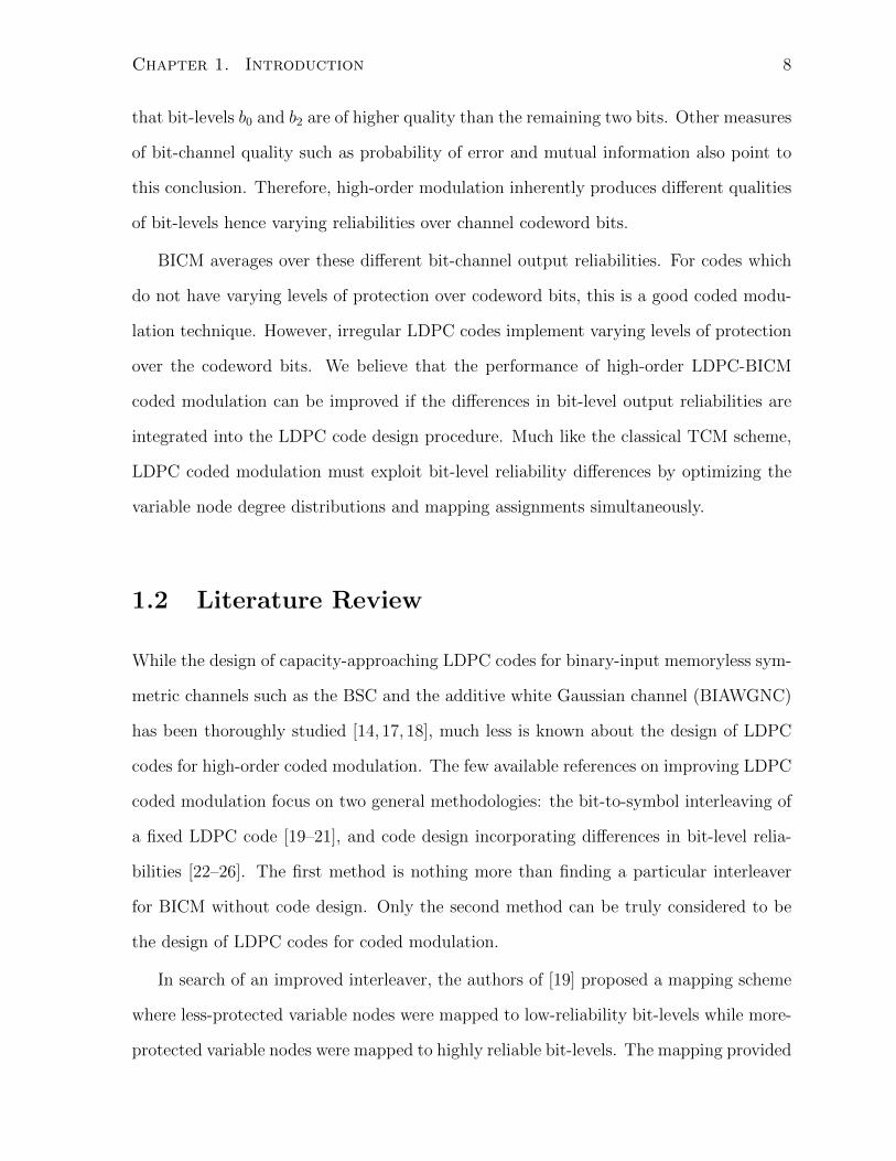
a bipartite graph called Tanner graph [13]. An example is shown in Fig. 1.2 for the
following parity-check matrix
H =
1 0 0 1 1 0 1
0 1 0 1 0 1 1
0 0 1 0 1 1 1
. (1.3)
The circles in Fig. 1.2 are called variable nodes and represent the columns of H. The
squares are called check nodes and represent the rows of H. The edges of the Tanner
+ + +
Figure 1.2: Tanner graph for parity check matrix in Eqn. 1.3.
Chapter 1. Introduction 6
graph connect codeword bits to the parity-check equations to which they belong.
The total number of edges that each variable/check node possesses is called the de-
gree of the variable/check node, corresponding to the number of non-zero entries in a
column/row of the parity-check matrix. If all variable nodes have the same degree, the
LDPC code is called regular. LDPC codes with variable nodes of different degrees are
called irregular codes. All capacity-approaching LDPC codes are irregular [14,15].
Decoding of LDPC codes uses the sum-product algorithm [16]. At the start, each vari-
able node receives a reliability measure from the demapper and sends it to neighbouring
checks. At the check nodes, the reliabilities are updated according to how well they sat-
isfy the parity-check constraints. After a complete iteration, variable nodes re-evaluate
their reliabilities according to repetition code constraints. This “message passing” action
continues until the variable node reliabilities are sufficiently high for a hard decision or
a maximum number of iterations has been reached.
We now outline the argument for seeking to improve the design of LDPC codes for
BICM systems. As repetition codes, LDPC variable nodes of different degrees offer dif-
ferent levels of error correction capability. High-degree variable nodes behave as very
long repetition codes and therefore are extremely reliable. However their low rates de-
crease the overall code rate significantly. On the other hand, degree 2 variable nodes
offer essentially no error correction but have the highest rate of all repetition codes. In
a capacity-approaching irregular LDPC code, there exists an inherent variation among
the different codeword bits.
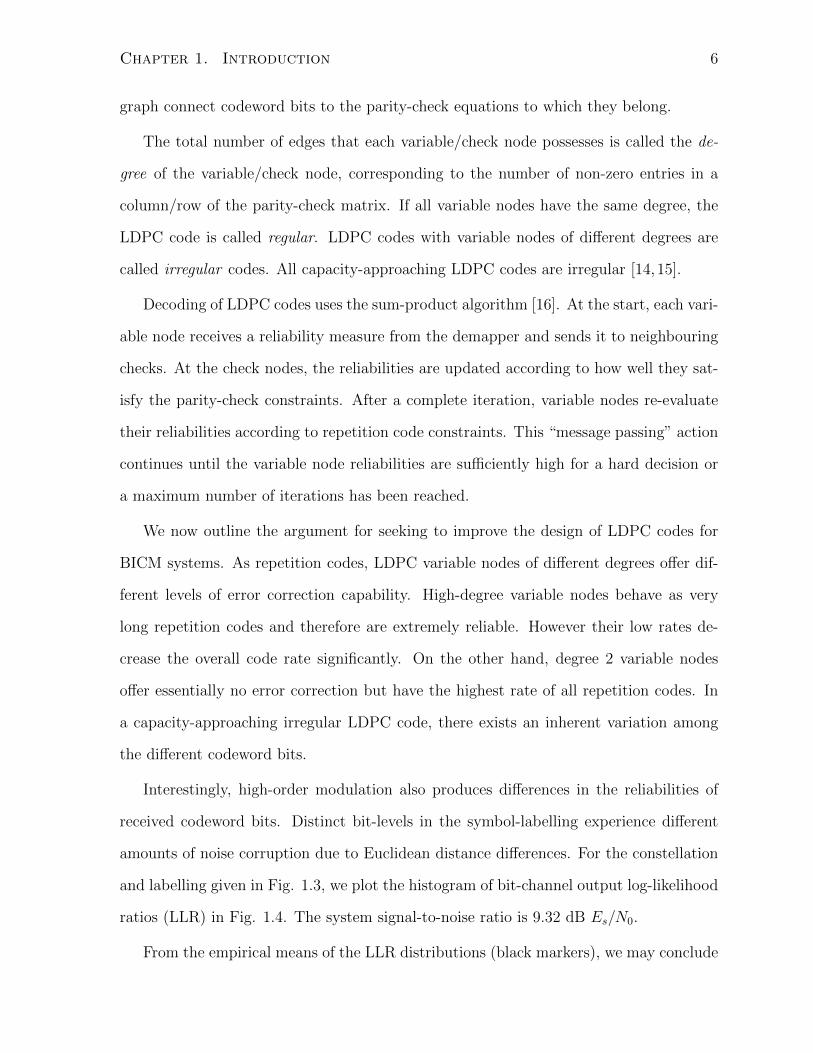
Interestingly, high-order modulation also produces differences in the reliabilities of
received codeword bits. Distinct bit-levels in the symbol-labelling experience different
amounts of noise corruption due to Euclidean distance differences. For the constellation
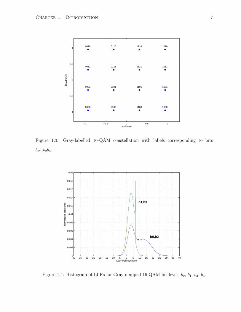
and labelling given in Fig. 1.3, we plot the histogram of bit-channel output log-likelihood
ratios (LLR) in Fig. 1.4. The system signal-to-noise ratio is 9.32 dB Es/N0.
From the empirical means of the LLR distributions (black markers), we may conclude
Chapter 1. Introduction 7
−1 −0.5 0 0.5 1
−1
−0.5
0
0.5
1
In−Phase
Qua
drat
ure
0000
0001
0011
0010
0100
0101
0111
0110
1100
1101
1111
1110
1000
1001
1011
1010
Figure 1.3: Gray-labelled 16-QAM constellation with labels corresponding to bits
b0b1b2b3.
−40 −35 −30 −25 −20 −15 −10 −5 0 5 10 15 20 25 30 35 400
0.002
0.004
0.006
0.008
0.01
0.012
0.014
0.016
0.018
0.02
Log−likelihood ratio
Nor
mal
ized
occ
uran
ce
b1,b3
b0,b2
Figure 1.4: Histogram of LLRs for Gray-mapped 16-QAM bit-levels b0, b1, b2, b3.
Chapter 1. Introduction 8
that bit-levels b0 and b2 are of higher quality than the remaining two bits. Other measures
of bit-channel quality such as probability of error and mutual information also point to
this conclusion. Therefore, high-order modulation inherently produces different qualities
of bit-levels hence varying reliabilities over channel codeword bits.
BICM averages over these different bit-channel output reliabilities. For codes which
do not have varying levels of protection over codeword bits, this is a good coded modu-
lation technique. However, irregular LDPC codes implement varying levels of protection
over the codeword bits. We believe that the performance of high-order LDPC-BICM
coded modulation can be improved if the differences in bit-level output reliabilities are
integrated into the LDPC code design procedure. Much like the classical TCM scheme,
LDPC coded modulation must exploit bit-level reliability differences by optimizing the
variable node degree distributions and mapping assignments simultaneously.
1.2 Literature Review
While the design of capacity-approaching LDPC codes for binary-input memoryless sym-
metric channels such as the BSC and the additive white Gaussian channel (BIAWGNC)
has been thoroughly studied [14, 17, 18], much less is known about the design of LDPC
codes for high-order coded modulation. The few available references on improving LDPC
coded modulation focus on two general methodologies: the bit-to-symbol interleaving of
a fixed LDPC code [19–21], and code design incorporating differences in bit-level relia-
bilities [22–26]. The first method is nothing more than finding a particular interleaver
for BICM without code design. Only the second method can be truly considered to be
the design of LDPC codes for coded modulation.
In search of an improved interleaver, the authors of [19] proposed a mapping scheme
where less-protected variable nodes were mapped to low-reliability bit-levels while more-
protected variable nodes were mapped to highly reliable bit-levels. The mapping provided
Chapter 1. Introduction 9
0.15-0.20 dB of improvement at no complexity increase. Intuitively, the improvement may
have been the result of allowing the most-reliable messages to propagate widely from high-
degree variable nodes. In [20], a mapping was proposed to minimize the connections of
each check node to variable nodes with low-reliability channel output, resulting in 0.3-0.7
dB of improvement. Finally, [21] proposed an improved interleaver for the DVB-S2 LDPC
code after taking into account the bit-level reliability differences. These mapping-based
methods certainly improved LDPC-BICM performance, but since the underlying LDPC
code was fixed the improvement was limited.
The most significant work on the design of LDPC codes for coded modulation has
been [22]. The work applies density evolution [14] to design LDPC codes for the dis-
tinct bit-channels of MLC and BICM. The problem is reduced to several binary LDPC
code designs. In [23] a powerful class of low-complexity, low error-floor LDPC codes
based on protographs are applied to high-order modulation with impressive performance.
Together, the references [22, 23] provide the most significant references for our work.
In [27, 28] LDPC codes are only used for low to medium quality bit channels, while
very high quality bit-channels are either uncoded or protected by very simple classical
codes. In [24–26], the multi-edge-type concepts are used in LDPC coded modulation.
Multi-edge-type LDPC codes [29, pp. 382-397] can incorporate the distinct bit-channel
reliabilities into code optimization. They also give the designer flexible control over code
structure to trade-off between complexity and performance. Although [24–26] did allude
to multi-edge ideas, they fall short of providing a specific multi-edge parameterization
with efficient analysis and design techniques. The key contribution of this thesis is the
design of multi-edge-type LDPC codes for LDPC-BICM.
Chapter 1. Introduction 10
1.3 Thesis Outline
Ch. 2 provides all the necessary technical background used in the rest of this thesis.
The target system model, fundamentals of LDPC design, density evolution and extrinsic
information transfer (EXIT) charts are a few of the topics reviewed in the chapter. Ch.
3 develops the multi-edge LDPC code design technique for coded modulation and forms
the main body of the thesis. The development follows from the initial specialization
of the multi-edge parameterization, to the multi-dimensional EXIT chart method for
analyzing such ensembles, to the innovative technique for code design based on the multi-
dimensional EXIT chart. Results of the new LDPC coded modulation design technique
are given in Ch. 4 in terms of both the ensemble thresholds and finite-length simulations.
Ch. 5 concludes the thesis and provides directions for future work.
Chapter 2
Technical Background
The goal of this chapter is to provide a comprehensive review of the technical knowledge
required for understanding the rest of the thesis. Sec. 2.1 describes the target system.
Several alternatives are discussed and justifications are given for choosing to limit the
scope of the thesis to one system. Binary LDPC analysis and design techniques are
reviewed in Sec. 2.2. A thorough understanding of the details and intuition of these
techniques is essential since the solutions developed in this thesis are based on these
binary design techniques. Lastly, Sec. 2.3 provides details on multi-edge-type LDPC
codes.
Throughout this thesis, bold font always denotes a vector quantity of length clear
from context. A bold constant denotes a vector of repeated entries, all of which are
equal to the indicated value. For example, 1 = (1, . . . , 1). A bold variable either denotes
a vector of variables, for example x = (x1, . . . , xn) or a vector field function f(x) =
(f1(x), . . . , fn(x)). The difference between them will be clear from context.
2.1 Target System
We now describe the system at which the design techniques given in this thesis are
aimed. As illustrated in Fig. 2.1, the source of the target system generates a sequence of
11
Chapter 2. Technical Background 12
ENC MAP
n
DMAP DECm c x y L c
Figure 2.1: Target system block diagram for the baseband-equivalent discrete-time com-
plex AWGN channel.
uniformly distributed independent and identically distributed binary random variables.
The channel code encoder takes k source bits per input block and maps them to a length
n (where n ≥ k) codeword c from the channel codebook C. The code rate is r = k/n.
A mapping function µ maps each codeword c to a sequence of modulation symbols
x, where each symbol xi is selected from the constellation X . In M bits per symbol
modulation, there are 2M distinct points in the constellation. Assuming n is a multiple
of M , the sequence x contains n/M symbols. For an arbitrary constellation labelling
scheme, let m = (0, . . . ,M − 1) index the bit-levels of the labelled constellation and let
bmi denote the m-th bit in the label of the transmitted symbol xi.
The sequence of symbols x, in discrete-time baseband-equivalent representation of
bandpass transmission, is corrupted by complex additive white Gaussian noise n = nI +
jnQ of variance σ2 = N0/2 per dimension, where N0/2 is the two-sided power spectral
density of the Gaussian noise. Note that all simulations in this thesis are performed
by assuming unity average symbol energy while scaling noise variance to the desired
signal-to-noise ratio.
At the receiver, the received sequence y = x + n is demapped by taking the bit-wise
log-likelihood ratio (LLR)
LMi+m = logP (yi|bmi = 0)
P (yi|bmi = 1)(2.1)
where i = (0, . . . , n/M − 1) indexes the received sequence y.
The uncoded maximum-likelihood decision rule is to decide 0 if LMi+m > 0, decide 1
if LMi+m < 0 and decide 0 or 1 at random with equal probability if LMi+m = 0.
Chapter 2. Technical Background 13
For complex additive white Gaussian channel with N0 = σ2 the LLR is given by
LMi+m = log
∑a∈X 0
m
exp
(− 1
N0
‖yi − a‖2)
∑b∈X 1
m
exp
(− 1
N0
‖yi − b‖2) . (2.2)
where X 0m and X 1
m partition the signalling constellation X into sets of points where bm = 0
and bm = 1, respectively.
The length n sequence L is decoded by the channel code decoder to the decoded word
c. A bit error occurs if ci 6= ci for some i, a frame error occurs if one or more bit errors
occur in the decoded word. After correct decoding, the transmitted message m can be
extracted from c if C is systematic. In this thesis, we judge the system error performance
only by comparing c to c.
2.1.1 IID channel adapter
As will be explained in Sec. 2.2, it is highly desirable for the bit-wise channels from
the transmitted codeword bits ci to the demapped LLR bit reliabilities Li to be output
symmetric. By definition, a binary-input channel is output symmetric if
P (Li|ci = 0) = P (−Li|ci = 1). (2.3)
High-order modulation systems are in general not output symmetric. A work-around
to this difficulty was introduced in [22] by inserting independent and identically dis-
tributed (iid) channel adapters into the system. At the transmitter, the iid channel
adapter XORs codeword c with a random binary sequence u generated from identically
distributed, uniform Bernoulli random variables. At the receiver, the sequence L is multi-
plied bit-wise by 1−2u. It is easy to verify that these two operations produce bit-channel
output symmetry while maintaining the same bit-channel capacity as the original sys-
tem. For proof please see the reference [22]. Note that iid channel adapters can be easily
Chapter 2. Technical Background 14
implemented in practice using synchronized pseudo-random binary sequence generators
at the transmitter and receiver.
2.1.2 Non-iterative vs. Iterative demapping
The system in Fig. 2.1 performs the single demap and decode operation used in BICM
systems. In MLC/MSD, the decoders for the lower bit-levels pass decoded bit informa-
tions back to the demapper to assist the next bit-level decoder. As mentioned, MSD can
achieve a capacity higher than non-iterative demapping. However, it has been shown
in [5] that if binary-reflected Gray labelling (BRGL) is used to label the constellation,
then the difference between the iterative and non-iterative demapping schemes is ex-
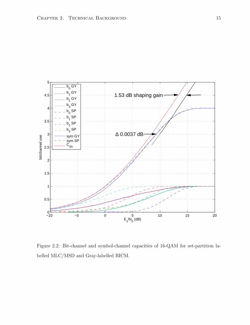
tremely small at high code rates. Fig. 2.2 plots the bit-channel and symbol-channel
capacities for 16-QAM under iterative and non-iterative decoding. The iterative scheme
is labelled using set-partition while non-iterative scheme uses BRGL. Note the small
difference (0.0037 dB) between MLC/MSD and BICM at rate 3/4.
The three types of capacities shown in Fig. 2.2 should be carefully distinguished.
The ultimate Shannon limit (red curve) is the capacity achieved under a continuous,
capacity-achieving input distribution with iterative demapping. The iterative demap-
ping capacity (dashed blue curve) can be achieved under discrete, uniformly distributed
16-QAM constellation with iterative demapping. The non-iterative demapping capacity
(solid blue curve) can be achieved under discrete, uniformly distributed 16-QAM constel-
lation without iterative demapping. We will always refer to the non-iterative demapping
capacity in this thesis unless otherwise noted.
Iterative demapping requires higher receiver complexity and latency. In light of the
negligible loss in capacity at the operating point marked in Fig. 2.2, we are justified to
focus on the low-complexity non-iterative Gray-labelled BICM scheme.
Chapter 2. Technical Background 15
−10 −5 0 5 10 15 200
0.5
1
1.5
2
2.5
3
3.5
4
4.5
5
Es/N
0 (dB)
bit/c
hann
el u
se
b
0 GY
b1 GY
b2 GY
b3 GY
b0 SP
b1 SP
b2 SP
b3 SP
sym GYsym SPC
Sh
1.53 dB shaping gain
∆ 0.0037 dB
Figure 2.2: Bit-channel and symbol-channel capacities of 16-QAM for set-partition la-
belled MLC/MSD and Gray-labelled BICM.
Chapter 2. Technical Background 16
2.1.3 Shaping
The gap between the ultimate Shannon limit and MLC/MSD capacity is due to the use
of a discrete, uniformly-distributed M -QAM constellation for the continuous-input com-
plex AWGN channel. From information theory we know the capacity-achieving input
distribution for this channel is a two-dimensional circularly symmetric Gaussian distri-
bution. The technique of approximating this ideal input distribution using a discrete
distribution is called shaping [30, 31]. An asymptotic shaping gain of 1.53 dB can be
achieved as shown in Fig. 2.2. We neglect shaping in our system to limit the scope of our
research. This simplification has also been made in all of prior works cited in Sec. 1.2.
We believe that shaping techniques can be applied to our code designs without affecting
the coded modulation gains.
2.2 Analysis and Design of Binary LDPC Codes
In this section we review well-known design and analysis techniques for capacity-approaching
irregular LDPC codes. Asymptotic ensemble analysis using density evolution and its ap-
proximation using extrinsic information transfer (EXIT) charts is explained in detail.
2.2.1 Ensemble-based design and density evolution
An irregular LDPC code of length n is fully specified by the number of variable nodes
and their degrees, the number of check nodes and their degrees, and the edge connections
between variable and check nodes. The number of variable and check nodes and their
degrees can be conveniently represented by using degree distribution polynomials
Λ(x) =dv∑i=1
Λixi , P (x) =
dc∑i=2
Pixi (2.4)
where dv and dc are maximum variable and check node degrees, Λi and Pi are the number
of variable and check nodes of each degree. Note that check degrees are greater or equal
Chapter 2. Technical Background 17
to 2 since a parity check equation of 1 term is useless. The total number of variable
nodes is Λ(1) = n and of check nodes is P (1) = (1− r)n.
It is more useful to normalize (2.4) by the number of variable and check nodes. We
define the node-perspective normalized degree distribution polynomials
L(x) =Λ(x)
Λ(1), R(x) =
P (x)
P (1). (2.5)
Node-perspective indicates that the coefficient in each term of the degree polynomial
denotes the fraction of nodes of that degree. An alternative edge-perspective degree
distribution polynomial indicates that the coefficients refer to the fraction of edges (in
total number edges) that are connected to nodes of that degree. It is easy to convert
node-perspective to edge-perspective degree distribution polynomials by
λ(x) =L′(x)
L′(1), ρ(x) =
R′(x)
R′(1)(2.6)
where ′ denotes differentiation.
Converting back to node-perspective degree distribution polynomials is achieved by
L(x) =
∫ x0λ(s)ds∫ 1
0λ(s)ds
, R(x) =
∫ x0ρ(s)ds∫ 1
0ρ(s)ds
. (2.7)
An ensemble is the set of all parity-check matrices (equivalently Tanner graphs) that
satisfy the degree distribution polynomials. By “satisfy”, we mean satisfy to within some
small tolerance, since in finite block-length it is often impossible to exactly satisfy the
distribution polynomials. Consider the degree of a node to be the number of “sockets”
it has available for edges to plug into. An edge-count constraint L′(1) = R′(1) is placed
on the variable and check degree distribution polynomials to ensure an equal number
of sockets on both sides. Let π be a permutation for a particular connection of edges
between variable node sockets and check node sockets. An ensemble is defined to be the
collection of all Tanner graphs which satisfy the degree distribution polynomials, under
all possible permutations π, and all possible channel outputs [18].
Chapter 2. Technical Background 18
The channel outputs are assumed to be independent between all codeword bits. The
bit-channel is assumed to be output symmetric as defined in (2.3). For a symmetric
channel, one can show that assuming only the all-zeros codeword is sent is equivalent
in performance to assuming all possible codewords are sent [29, pp. 215-216]. Hence
under the symmetric channel assumption, the ensemble also encompasses all possible
transmitted codewords. This is why iid channel adapters are necessary in our target
system. Ensemble-based analysis cannot be used for code design if the bit-channels are
not output symmetric.
The sum-product algorithm
Ensemble-based analysis evaluates the expected probability of message errors for some
decoding algorithm, averaged over all Tanner graphs and channel outputs in the ensem-
ble. The decoding algorithm for LDPC codes in AWGN is a specialized instance of the
message-passing sum-product algorithm [16] called Belief Propagation (BP) [4].
For any variable node vi in a LDPC code Tanner graph, denote its channel output
LLR by µi. Let J denote the indices of its neighbouring check nodes. For any check
node cj, let I denote the indices of its neighbouring variable nodes. Let µvi→j and µci→j
represent the messages passed from variable and check node of index i to a node of index
j. Initially, all µci→j = 0 and all µvi→j = µi.
In subsequent iterations, the variable node update equation is
µvi→j =∑j′∈J\j
µcj′→i + µi, ∀j ∈ J . (2.8)
The check node update equation is
µcj→i = 2 tanh−1
∏i′∈I\i
tanh
(µvi′→j
2
) , ∀i ∈ I. (2.9)
A full decoding iteration includes one execution of variable and check updates. At
Chapter 2. Technical Background 19
the end of every iteration, a hard decision is made for variable vi based on µvi→j + µcj→i
using the decision rule from Sec. 2.1. Decoding ends when the hard-decision codeword
passes parity check or a maximum number of decoding iterations has been reached.
Concentration, decoding-tree and density evolution
Several key results justify ensemble-based analysis and its main tool, density evolution.
The concentration theorem [18] states that if P n(l) is the expected fraction of incorrect
messages passed during the l-th decoding iteration for a block-length n code ensemble,
then the probability of the actual fraction of incorrect messages for a sample code of the
ensemble being outside of (P n(l)− δ, P n(l) + δ) tends to 0 exponentially with n, for any
δ > 0.
Given the concentration theorem, the problem of analyzing the error performance of
a particular code Tanner graph is converted to analyzing the expected performance of all
Tanner graphs in the ensemble. At first this appears to be an even more difficult problem,
but the expansion of a code to its ensemble allows for a second simplifying theorem to
be applied.
A second key theorem in [18] states that the ensemble expected fraction of incorrect
messages P n(l) converges to P∞(l) as n tends to infinity, where P∞(l) is the fraction
of incorrect messages passed during iteration l assuming the decoding neighbourhood of
depth l is cycle-free.
The decoding neighbourhood of depth l for a variable node vi is the recursive expan-
sion of edges and neighbouring nodes of vi in l decoding iterations. An additional level
of check and variable nodes is added with every iteration. A length 2l cycle exists if vi
appears in its own decoding neighbourhood of depth l. Intuitively, the presence of cycles
means the message received by vi after l decoding iterations is necessarily dependent on
previous messages from vi, hence messages are correlated. Correlated message passing is
extremely difficult to analyze. The convergence of ensemble expectation to the cycle-free
Chapter 2. Technical Background 20
case allows for the assumption that all messages are independent, greatly simplifying
analysis. The results for the cycle-free graph directly apply to the ensemble expectation,
since they are equal as n tends to infinity.
The fraction of error messages of the cycle-free graph is analyzed using Density Evo-
lution (DE) [18]. DE tracks all messages in the BP decoding algorithm for the cycle-free
graph realization of the code ensemble, over all possible channel outputs and transmitted
codewords. As the name suggests, DE operates on probability densities of the channel
outputs and messages.
Let P0 denote the density of the channel output LLR. Initially, the variable nodes all
send their channel output, therefore the density of the µvi→j messages is P0. At the check
nodes, let Γ() and Γ−1() be a transform and its inverse that implements (2.9) and allows
for the message calculation in the transform domain to be a sum. Such a transform is
given in [18]. For a degree i check node, with independent incoming messages, the output
message density is given by
Γ−1(Γ(P0)⊗(i−1)) (2.10)
where⊗ denotes convolution and exponentiation is a shorthand for repeated convolutions.
Averaging over all check node degrees and their respective edge-perspective distribu-
tion coefficients, we obtain the µcj→i message density after 1 iteration as
Q1 = Γ−1(ρ(Γ(P0))) = Γ−1
(dc∑i=2
ρiΓ(P0)⊗(i−1)
). (2.11)
In the cycle-free decoding neighbourhood, all messages remain independent after node
updates. Therefore the variable message density after 1 iteration is
P1 = P0 ⊗ λ(Q1) = P0 ⊗dv∑i=1
λ⊗(i−1)i . (2.12)
For any iteration l, the recursive density update for µvi→j messages is
Chapter 2. Technical Background 21
Pl = P0 ⊗ λ(Γ−1(ρ(Γ(Pl−1)))). (2.13)
The density evolution threshold for the AWGN channel is defined to be σ∗ such that
Pl → 0 as l →∞ for all σ < σ∗. In [15] a quantized version of density evolution named
discrete density evolution is given with good implementation and numerical stability
characteristics. All thresholds reported in this thesis are evaluated using discrete density
evolution.
To summarize, in ensemble-based LDPC code analysis, for a given pair of variable and
check node degree distributions, the goal is to evaluate the expected fraction of incorrect
messages for the ensemble of all code Tanner graphs, channel outputs and transmitted
codewords. At large block-lengths, the faction of incorrect messages of any specific code
Tanner graph is concentrated around the ensemble expectation. The expectation is shown
to be asymptotically equal to the fraction of incorrect messages of the cycle-free decoding
neighbourhood, which can be analytically determined using density evolution.
Gaussian-approximated density evolution
Density evolution is an effective analytical tool for finding the threshold of LDPC code
ensembles parameterized by degree distribution pairs. However, as a synthesis method
to find good degree distribution pairs it is overly complex to be useful in optimization.
Originally, [14] used the genetic algorithm differential evolution [32] to optimize degree
distribution pairs. Such heuristic algorithms are prone to being trapped in local minima
and does not give any convergence guarantee. In addition, since every optimization
iteration requires many threshold evaluations, this leads to extremely high runtimes.
The complexity of density evolution can be reduced if the message densities (Pl, Ql)
are approximated by using symmetric Gaussian densities. Intuitively, since variable node
updates are convolutions of independent input message densities, by the central limit
theorem [33] the output message density is approximately Gaussian for high node degrees.
Chapter 2. Technical Background 22
For the purpose of this discussion, we define a symmetric Gaussian density to be a
Gaussian density with σ2 = 2µ [29]. Consequently, only one parameter µ is needed
to fully specify the density function. This Gaussian-approximated density evolution
(GA-DE) was introduced in [34] where the authors found degree distribution pairs with
thresholds within 0.02 dB of full density evolution designs.
The key simplifying aspect of GA-DE is the node update equations are no longer
operations on densities but on the single representative parameter. The convolution of
symmetric Gaussian densities with mean µ at a degree i variable node simply results in
an output Gaussian of mean (i−1)µl−1 +µ0 where µ0 is the mean of the channel output.
The check node update can be similarly condensed into an expression involving the input
message means only. An entire GA-DE iteration can be expressed from the perspective
of the average variable output message mean µvl as
µvl = f(µv0, µvl−1) (2.14)
where f is the single-variable function model of (2.13). It has been shown in [34] that
the condition f(µv0, µvl−1) > µvl−1 is necessary and sufficient to ensure convergence to zero
incorrect messages in GA-DE. More importantly, this convergence condition is linear,
thus allowing optimization to be achieved by using efficient linear programming.
GA-DE was an early instance of single-parameter approximations of density evolu-
tion. The idea of single-parameter approximation is to apply the symmetric Gaussian
approximation to reduce the cumbersome operations of (2.13) to iterated functions of one
parameter. Powerful optimization tools can then be applied to the iterated functions.
The single-parameter approximation design technique was further studied in [35] using
a semi-Gaussian approximation. The modification improved threshold accuracy and de-
sign flexibility as the original GA-DE did not work well for variable degrees greater than
10 [34].
Chapter 2. Technical Background 23
2.2.2 Extrinsic information transfer charts
The most widely used single-parameter approximation of density evolution is the extrinsic
information transfer (EXIT) technique. In essence, EXIT uses the “extrinsic information”
parameter as the single-parameter approximation for GA-DE. The definition of extrinsic
information is based on the extrinsic processing principle of iterative decoding algorithms.
Extrinsic processing is evident in BP update equations (2.8), (2.9) where the out-going
message from node i to node j always excludes the incoming message from node j to
node i. On a cycle-free decoding graph, the extrinsic processing principle ensures that a
node will never receive messages dependent on itself.
Assume a variable node initially receives an incorrect channel output LLR, to correct
this bit it must eventually receive sufficiently correct extrinsic messages. This means the
mutual information between the extrinsic messages of bit i and the value of bit i must
eventually converge to 1 as l→∞. The mutual information is defined in [36] as
I(X;L) = H(X)−H(X|L)
= 1−∫∞−∞
e−(ξ−σ2/2)2/2σ2√2πσ2
log2 [1 + e−ξ]dξ
≡ J(σ)
(2.15)
where X is the uniform binary random variable representing a codeword bit and L is the
demapped LLR output from a symmetric AWGN channel of variance σ2.
Using this conversion between σ and extrinsic mutual information, the update equa-
tions for EXIT-based GA-DE are
Ivl =dv∑i=1
λiJ
(√(i− 1)[J−1(Icl )]
2 + σ2ch
), (2.16)
Icl = 1−dc∑i=2
ρiJ(√
(i− 1)[J−1(1− Ivl−1)]2)
(2.17)
where v, c superscripts indicate the extrinsic mutual information updates due to variable
or check nodes, l is the decoding iteration, and σ2ch is the channel output LLR variance.
Chapter 2. Technical Background 24
The functions J(σ) and J−1(I) can be pre-calculated or approximated as in [36]. Note
the extrinsic informations are averaged over different variable and check node degrees.
An approximation is made in (2.17) to find the check node mutual information update
based on duality between parity-check and repetition codes. For a full justification please
refer to [36, 37]. The condition for successful decoding is Ivl → 1 as l → ∞. Successful
decoding is defined to be the existence of a sequence of codes of block-length n such that
the probability of bit error goes to 0 as n → ∞ and l → ∞. Conversely, decoding is
unsuccessful for a code ensemble if the probability of bit error is bounded away from 0
as n→∞ and l→∞ [29].
Combining (2.16) and (2.17) into a function f , the equivalent convergence condition
for successful decoding is [35]
f(Iv, σ2ch) > Iv, ∀Iv ∈ [J(σch), 1) (2.18)
Observe that (2.16) is a linear combination with coefficients λi, so that (2.18) can be
re-written as
Ivl =dv∑i=1
λifi(Ivl−1, σ
2ch), (2.19)
where fi captures the extrinsic mutual information transfer of only degree i variable nodes
and one particular check degree. We call these functions elementary EXIT functions. The
code design optimization problem is a linear programming problem that maximizes the
code rate 1− (∑ρj/j/
∑λi/i) over variable node degree distributions λi given by
maxλi
∑i≥1
λii
λi ≥ 0∑i≥1 λi = 1∑
i≥1 λifi(Ivl−1) > Ivl−1, ∀Ivl−1 ∈ [J(σch), 1).
(2.20)
Chapter 2. Technical Background 25
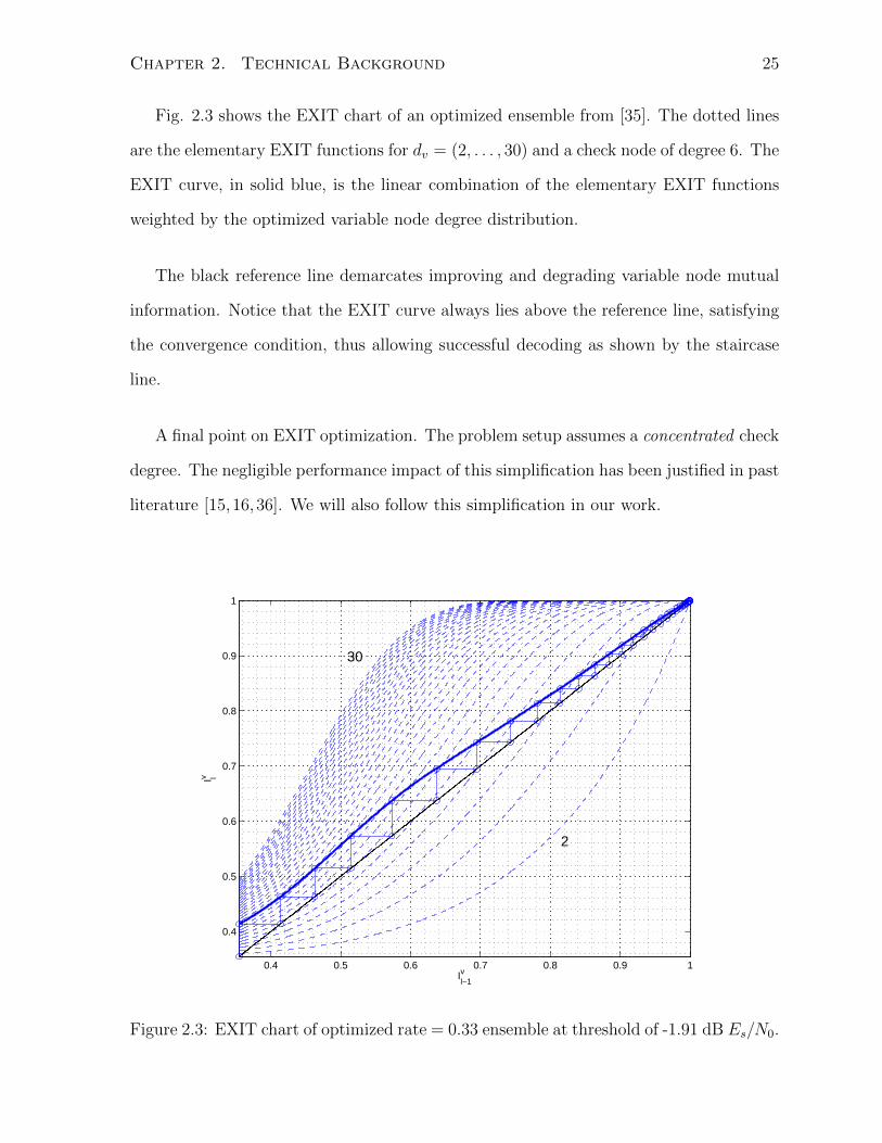
Fig. 2.3 shows the EXIT chart of an optimized ensemble from [35]. The dotted lines
are the elementary EXIT functions for dv = (2, . . . , 30) and a check node of degree 6. The
EXIT curve, in solid blue, is the linear combination of the elementary EXIT functions
weighted by the optimized variable node degree distribution.
The black reference line demarcates improving and degrading variable node mutual
information. Notice that the EXIT curve always lies above the reference line, satisfying
the convergence condition, thus allowing successful decoding as shown by the staircase
line.
A final point on EXIT optimization. The problem setup assumes a concentrated check
degree. The negligible performance impact of this simplification has been justified in past
literature [15,16,36]. We will also follow this simplification in our work.
0.4 0.5 0.6 0.7 0.8 0.9 1
0.4
0.5
0.6
0.7
0.8
0.9
1
Il−1v
I lv
2
30
Figure 2.3: EXIT chart of optimized rate = 0.33 ensemble at threshold of -1.91 dB Es/N0.
Chapter 2. Technical Background 26
2.3 Multi-edge-type LDPC Codes
The key motivation for the development of multi-edge-type LDPC codes is to impose
structure over the random single-edge-type code ensemble defined by pairs of variable
and check node degree distribution polynomials. Here we describe two examples where
prudently imposed structure leads to complexity reduction or performance improvement
over completely structureless code ensembles.
Given a maximum variable node degree, it has been observed that under density
evolution optimization, variable node degree distributions heavily utilize variable nodes
of the highest degree in order to achieve capacity-approaching performance [14]. In
practical implementation, the complexity of the decoder hardware scales directly with
the maximum variable degree. Therefore, it is desirable to reduce the maximum variable
degree while maintaining the capacity-approaching performance. High degree variable
nodes are appealing since they help to propagate any reliable intrinsic information and
extrinsic information that they are likely to produce. Under the purely random socket
assignment of single-edge-type LDPC codes, a very high variable node degree is required
to achieve this “spreading” effect with sufficiently high probability. However, if a code
designer imposes structure on maximum degree variable nodes, for example by avoiding
connections to many degree 2 nodes, then the same effect can be achieved with high
probability for a lower maximum variable degree [29, pp. 384-389].
A second example concerns degree 1 variable nodes in LDPC code ensembles. Since a
degree 1 variable node only sends its channel observation during message-passing decod-
ing, if it receives an erroneous channel observation then any check node it is connected
to is likely to pass on the erroneous message to its neighbouring variable nodes. It is
easy to see that if two or more degree 1 variable nodes are connected to the same check
node and a few receives erroneous channel observations, they will never be corrected
under message-passing decoding. Density evolution on a single-edge-type ensemble with
degree 1 variable nodes correctly gives a bit error probability bounded away from zero.
Chapter 2. Technical Background 27
For multi-edge-type code ensembles, the code designer can explicitly impose structure
on degree 1 variable nodes to eliminate the case where two or more are connected to the
same check node. With the extra structure, the bit error probability can be made to
go to zero for infinite block-length [29, pp. 394-397]. The inclusion of degree 1 variable
nodes brings many benefits such as lower error floor, improved decoding threshold, and
simpler implementation.
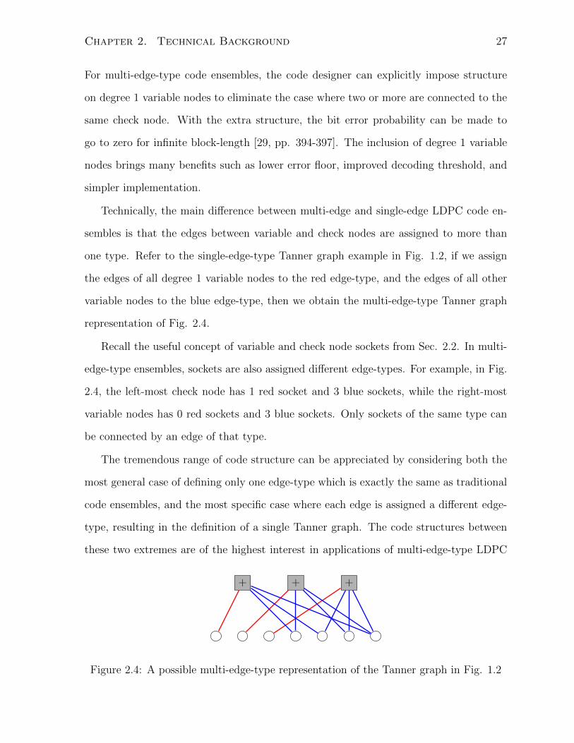
Technically, the main difference between multi-edge and single-edge LDPC code en-
sembles is that the edges between variable and check nodes are assigned to more than
one type. Refer to the single-edge-type Tanner graph example in Fig. 1.2, if we assign
the edges of all degree 1 variable nodes to the red edge-type, and the edges of all other
variable nodes to the blue edge-type, then we obtain the multi-edge-type Tanner graph
representation of Fig. 2.4.
Recall the useful concept of variable and check node sockets from Sec. 2.2. In multi-
edge-type ensembles, sockets are also assigned different edge-types. For example, in Fig.
2.4, the left-most check node has 1 red socket and 3 blue sockets, while the right-most
variable nodes has 0 red sockets and 3 blue sockets. Only sockets of the same type can
be connected by an edge of that type.
The tremendous range of code structure can be appreciated by considering both the
most general case of defining only one edge-type which is exactly the same as traditional
code ensembles, and the most specific case where each edge is assigned a different edge-
type, resulting in the definition of a single Tanner graph. The code structures between
these two extremes are of the highest interest in applications of multi-edge-type LDPC
+ + +
Figure 2.4: A possible multi-edge-type representation of the Tanner graph in Fig. 1.2
Chapter 2. Technical Background 28
codes.
In the rest of this section we overview the notation used to work with multi-edge-type
code ensembles, closely following the treatment in [29, pp. 382-397]. The emphasis will
be on the distinguishing features between single and multi-edge-type notations. It may
be helpful for the reader to review the single-edge-type notations in Sec. 2.2 to compare
with those introduced here.
The notation used to distinguish edge-types in multi-edge-type (MET) degree distri-
butions extends the placeholder variable x and node degree d to vectors x and d, where
each vector component refers to an edge-type. Whereas a single-edge-type check node of
degree 4 in the node-perspective is denoted by x4, a check node of 3 edge-types of degree
d = (2, 3, 4) is denoted in the node-perspective by x21x32x
43. In Fig. 2.4, the left-most
check node would be denoted by x11x32. A variable node in an MET ensemble has the
additional vector r specifying the channel output densities to which it is connected. A
variable node with 2 type 1 sockets and 2 type 2 sockets receiving the channel output
density 1 is denoted by x21x2xr1 while the same variable node receiving channel output
density 2 is denoted by x21x22r2. In addition to imposing structure, the ability to assign
different channel output densities to different variable nodes is another reason for using
MET ensembles in this work. Our goal is to exploit the different output densities of
bit-channels using inherent differences in LDPC codeword bit protection.
Throughout this thesis, the total number of edge-types is denoted by T and indexed
by k = (1, . . . , T ). The total number of distinct channel output densities is denoted by
S and indexed by s = (0, . . . , S). Note that there are S + 1 channel output densities,
however the s = 0 density corresponds to the channel output of a punctured variable node
which is not used in this work. All edge-type specific quantities such as the maximum
variable or check degree, or edge-perspective degree distribution, will be distinguished by
a superscript. For example d1v or λ1 are quantities of the edge-type 1. Finally, let ∂x be
a shorthand for the partial differentiation operator ∂∂x
.
Chapter 2. Technical Background 29
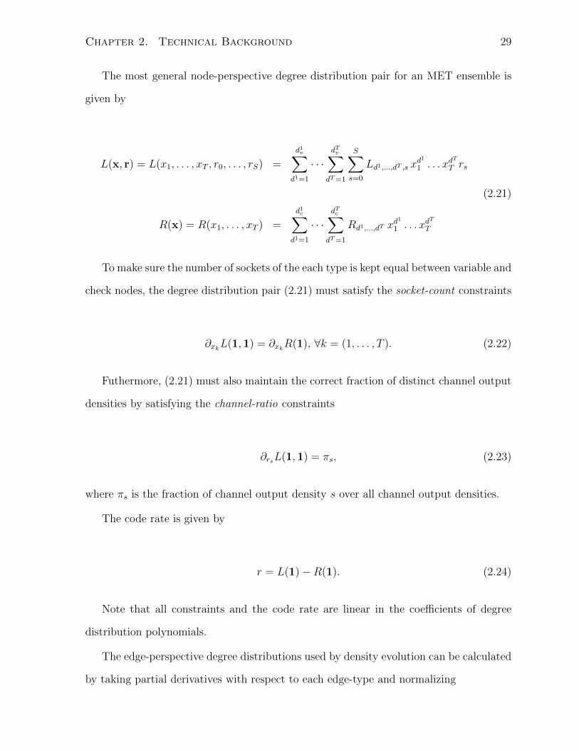
The most general node-perspective degree distribution pair for an MET ensemble is
given by
L(x, r) = L(x1, . . . , xT , r0, . . . , rS) =
d1v∑d1=1
· · ·dTv∑dT=1
S∑s=0
Ld1,...,dT ,s xd1
1 . . . xdT
T rs
R(x) = R(x1, . . . , xT ) =
d1c∑d1=1
· · ·dTc∑dT=1
Rd1,...,dT xd1
1 . . . xdT
T
(2.21)
To make sure the number of sockets of the each type is kept equal between variable and
check nodes, the degree distribution pair (2.21) must satisfy the socket-count constraints
∂xkL(1,1) = ∂xkR(1), ∀k = (1, . . . , T ). (2.22)
Futhermore, (2.21) must also maintain the correct fraction of distinct channel output
densities by satisfying the channel-ratio constraints
∂rsL(1,1) = πs, (2.23)
where πs is the fraction of channel output density s over all channel output densities.
The code rate is given by
r = L(1)−R(1). (2.24)
Note that all constraints and the code rate are linear in the coefficients of degree
distribution polynomials.
The edge-perspective degree distributions used by density evolution can be calculated
by taking partial derivatives with respect to each edge-type and normalizing
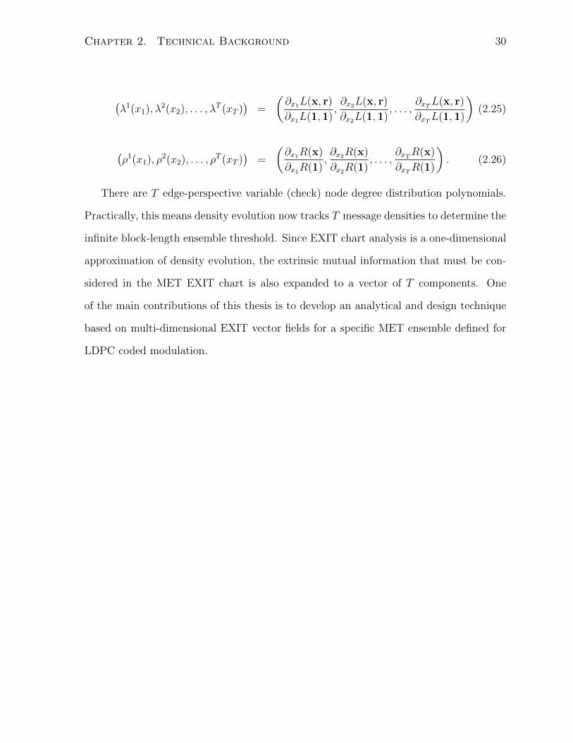
Chapter 2. Technical Background 30
(λ1(x1), λ
2(x2), . . . , λT (xT )
)=
(∂x1L(x, r)
∂x1L(1,1),∂x2L(x, r)
∂x2L(1,1), . . . ,
∂xTL(x, r)
∂xTL(1,1)
)(2.25)
(ρ1(x1), ρ
2(x2), . . . , ρT (xT )
)=
(∂x1R(x)
∂x1R(1),∂x2R(x)
∂x2R(1), . . . ,
∂xTR(x)
∂xTR(1)
). (2.26)
There are T edge-perspective variable (check) node degree distribution polynomials.
Practically, this means density evolution now tracks T message densities to determine the
infinite block-length ensemble threshold. Since EXIT chart analysis is a one-dimensional
approximation of density evolution, the extrinsic mutual information that must be con-
sidered in the MET EXIT chart is also expanded to a vector of T components. One
of the main contributions of this thesis is to develop an analytical and design technique
based on multi-dimensional EXIT vector fields for a specific MET ensemble defined for
LDPC coded modulation.
Chapter 3
Multi-edge LDPC Coded
Modulation
In this chapter we develop the main contributions of this thesis. In Sec. 3.1 the general
MET ensemble is reduced to a specific parameterization for LDPC coded modulation.
Thorough justifications are given for all simplifications. Sec. 3.2 develops the main
analytical tool for the specified MET ensemble: the multi-dimensional EXIT vector field.
Several properties of the vector field are proved. Code design using the multi-dimensional
EXIT vector field is accomplished after deriving the multi-edge-type convergence criterion
based on the fixed points of the iterated system.
3.1 Multi-edge Parameterization
We seek to leverage two important properties unique to multi-edge-type (MET) LDPC
framework in our coded modulation design. MET ensembles allow, as input, more than
one channel output density at variable nodes. This is precisely the desired property for
incorporating bit-level differences into the ensemble optimization process. Furthermore,
the expanded number of edge-types offers flexible control over the structure of the LDPC
ensemble. Structural features can be defined in the ensemble definition before optimiza-
31
Chapter 3. Multi-edge LDPC Coded Modulation 32
tion. Several reasons exist for imposing code structure, most common are to reduce
design and implementation complexity or to lower the error floor.
In this work, we specify a MET structure for complexity reduction. The number of free
coefficients in the general MET variable and check degree distribution polynomials (2.21)
grows exponentially with the number of edge-types. Taking into account the plausible
number of distinct channel output densities, for example 5 in the case of Gray-labelled
1024-QAM, optimizing the general degree distributions quickly becomes intractable.
We would like to simplify the parameterization to a manageable complexity without
sacrificing the desired properties of the MET framework. This can be achieved by first
assigning one edge-type to each distinct bit-channel output density. For example, in
Gray-labelled 16-QAM there are 4 bit-channels but only 2 distinct bit-channel output
densities, therefore only 2 edge-types are used; whereas for set-partition labelled 16-
QAM there are 4 distinct bit-channel output densities, requiring 4 edge-types in the
MET parameterization.
In addition, each variable node is restricted to have sockets of only one edge-type,
while different edge-type sockets are present at check nodes. We are inspired to make
this simplification by the MLC scheme, where a distinct LDPC code is optimized for each
bit-level in order to approach the capacity of the overall symbol channel. We extend the
idea by allowing variable node messages of different edge-types to interact at check nodes,
and more importantly, by optimizing the code across all bit-channels simultaneously.
With these two restrictions on the general MET ensemble, a flexible trade-off between
designing one code for an averaged channel (BICM) and designing distinct codes for dis-
tinct bit-channels (MLC) is achieved by our specific MET parameterization. The single,
optimized code under our MET parameterization will not only be properly matched to
each bit-channel, but also to the overall high-order modulation symbol channel. Fig. 3.1
(b) illustrates the specified MET parameterization for the case of 2 distinct bit-channels
such as Gray-labelled 16-QAM.
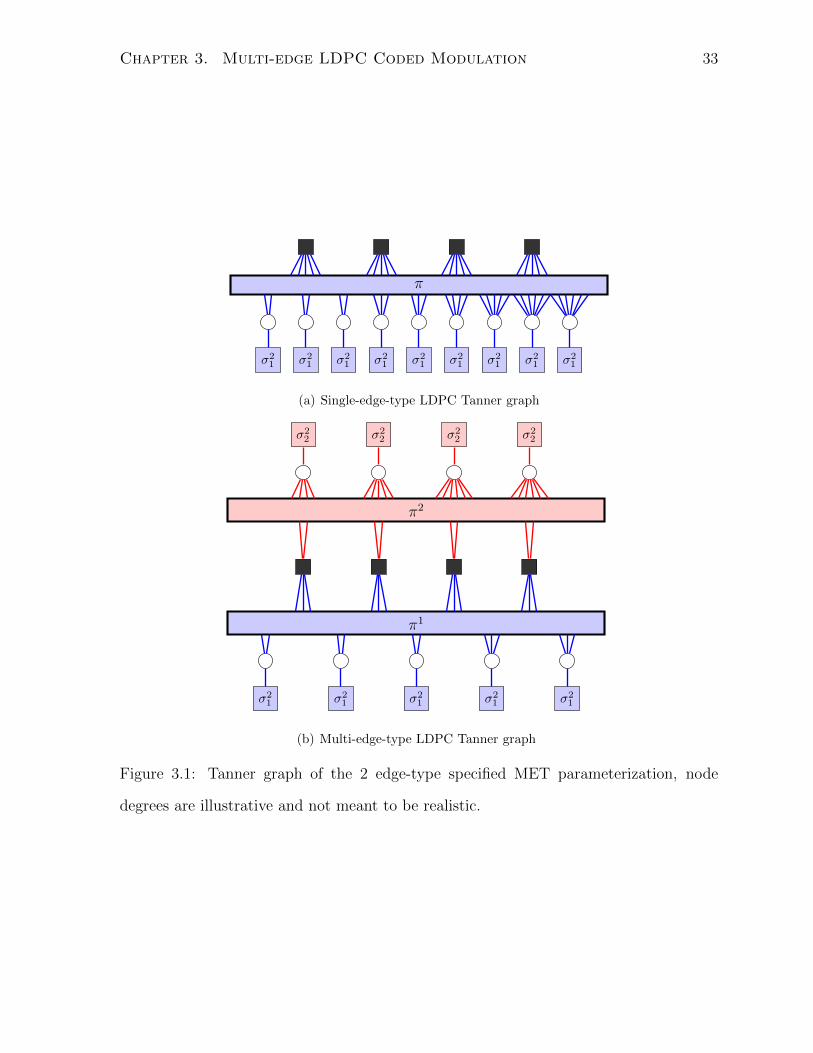
Chapter 3. Multi-edge LDPC Coded Modulation 33
σ21 σ2
1 σ21 σ2
1 σ21 σ2
1 σ21 σ2
1 σ21
π
(a) Single-edge-type LDPC Tanner graph
σ21 σ2
1 σ21 σ2
1 σ21
σ22 σ2
2 σ22 σ2
2
π1
π2
(b) Multi-edge-type LDPC Tanner graph
Figure 3.1: Tanner graph of the 2 edge-type specified MET parameterization, node
degrees are illustrative and not meant to be realistic.
Chapter 3. Multi-edge LDPC Coded Modulation 34
The variable degree distribution for the specific MET parameterization is
L(x1, . . . , xT , r1, . . . , rT ) =T∑k=1
dkv∑i=1
Li,kxikrk. (3.1)
The index k serves the dual purposes of indexing the edge-types and channel densities,
since they are the same under our specification. The bit-channel density of index k = 0
is removed since puncturing is not considered in this work. From (3.1) and Fig. 3.1 it is
clear that the MET parameterization from the variable node perspective is identical to
a single-edge-type parameterization.
In fact, if the check node degree distributions are specified such that no mixing of
edge-types can occur, the specific MET parameterization degenerates to the MLC scheme.
However, we do allow different edge-types at the check nodes, which allows messages from
different bit-channels to mix. As a final simplification, we require the total check node
degree dc be concentrated to only one value. The total check node degree is the number
of all sockets at a check node, regardless of type. Under this simplification, (2.21) can be
written as
R(x1, . . . , xT ) =∑
{d1,...,dT |d1+···+dT=dc}
Rd1,...,dT xd11 . . . xdTT . (3.2)
Even after concentrating to one total check degree, the check degree distribution
remains overly complex. The additional complication is in choosing the assignment of
check node sockets to different edge-types, under the same total degree. For 2 edge-types
and a total check degree of dc there are dc + 1 possible edge-type assignments. For more
than 2 edge-types the number of possible assignments grows rapidly, and is related to
the partition function P [dc] from number theory [38]. In order to gain insight into this
problem and to explore the possibility of concentrating to only one check node edge-type
assignment, we undertook an empirical study using simple MET LDPC ensembles with
2 edge-types.
Chapter 3. Multi-edge LDPC Coded Modulation 35
3.1.1 Check degree edge-type assignment
The goal of this study is to justify further simplifying the check node degree distribution
to a single term, given by
R(x1, . . . , xT ) = Rd1c ,...,dTcxd1c1 . . . x
dTcT , (3.3)
where d1c + · · ·+ dTc = dc is a chosen check degree edge-type assignment. Note the direct
use of dkc to denote the number of check sockets of type k, since only one term of the sum
is present.
The first code under study is the regular (3,6) ensemble, where the notation corre-
sponds to (dv,dc), of rate 1/2. For Gray-labelled 16-QAM with 2 distinct bit-channels,
the degree 6 check node can be split into (d1c , d2c) = {(0, 6), (1, 5), . . . , (6, 0)} over the
2 edge-types. However, since the variable node parameterization imposes a constraint
(2.22) on the number of edges of each type, we focus on the case of pairs of check degree
edge-type splits where the distribution coefficients can be directly found. For example,
the check degree distribution polynomial for the pair of assignments (0,6), (4,2) is
R(x1, x1) = R1x62 +R2x
41x
22, (3.4)
where R1,R2 are obtained by substituting (3.4) into (2.22) and solving the system. The
thresholds for all pairs of check node splits are given in Table 3.1, the pairs that do not
satisfy the edge-count constraint are marked by “-”.
The check node split pairing with the highest density evolution threshold is the sin-
gle symmetrical (3,3) split. The next highest threshold belongs to the pair of nearly-
symmetrical (2,4), (4,2) splits. From this simple example it appears that when the check
degree polynomial is restricted to pairs of edge-type assignments as in (3.4), concentrat-
ing to a single symmetrical split gives the highest threshold.
To see if the same property can be observed for an odd total check degree, we repeated
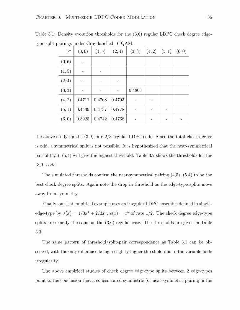
Chapter 3. Multi-edge LDPC Coded Modulation 36
Table 3.1: Density evolution thresholds for the (3,6) regular LDPC check degree edge-
type split pairings under Gray-labelled 16-QAM.
σ∗ (0, 6) (1, 5) (2, 4) (3, 3) (4, 2) (5, 1) (6, 0)
(0, 6) -
(1, 5) - -
(2, 4) - - -
(3, 3) - - - 0.4808
(4, 2) 0.4711 0.4768 0.4793 - -
(5, 1) 0.4439 0.4737 0.4778 - - -
(6, 0) 0.3925 0.4742 0.4768 - - - -
the above study for the (3,9) rate 2/3 regular LDPC code. Since the total check degree
is odd, a symmetrical split is not possible. It is hypothesized that the near-symmetrical
pair of (4,5), (5,4) will give the highest threshold. Table 3.2 shows the thresholds for the
(3,9) code.
The simulated thresholds confirm the near-symmetrical pairing (4,5), (5,4) to be the
best check degree splits. Again note the drop in threshold as the edge-type splits move
away from symmetry.
Finally, our last empirical example uses an irregular LDPC ensemble defined in single-
edge-type by λ(x) = 1/3x1 + 2/3x3, ρ(x) = x5 of rate 1/2. The check degree edge-type
splits are exactly the same as the (3,6) regular case. The thresholds are given in Table
3.3.
The same pattern of threshold/split-pair correspondence as Table 3.1 can be ob-
served, with the only difference being a slightly higher threshold due to the variable node
irregularity.
The above empirical studies of check degree edge-type splits between 2 edge-types
point to the conclusion that a concentrated symmetric (or near-symmetric pairing in the
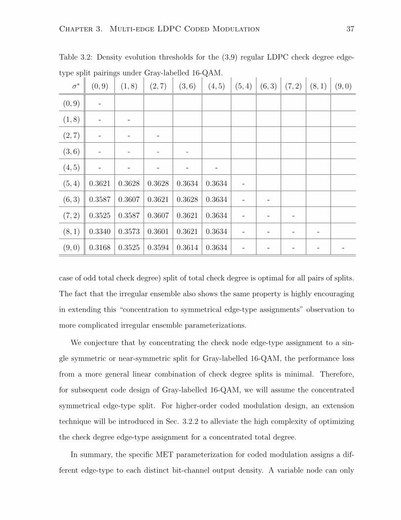
Chapter 3. Multi-edge LDPC Coded Modulation 37
Table 3.2: Density evolution thresholds for the (3,9) regular LDPC check degree edge-
type split pairings under Gray-labelled 16-QAM.
σ∗ (0, 9) (1, 8) (2, 7) (3, 6) (4, 5) (5, 4) (6, 3) (7, 2) (8, 1) (9, 0)
(0, 9) -
(1, 8) - -
(2, 7) - - -
(3, 6) - - - -
(4, 5) - - - - -
(5, 4) 0.3621 0.3628 0.3628 0.3634 0.3634 -
(6, 3) 0.3587 0.3607 0.3621 0.3628 0.3634 - -
(7, 2) 0.3525 0.3587 0.3607 0.3621 0.3634 - - -
(8, 1) 0.3340 0.3573 0.3601 0.3621 0.3634 - - - -
(9, 0) 0.3168 0.3525 0.3594 0.3614 0.3634 - - - - -
case of odd total check degree) split of total check degree is optimal for all pairs of splits.
The fact that the irregular ensemble also shows the same property is highly encouraging
in extending this “concentration to symmetrical edge-type assignments” observation to
more complicated irregular ensemble parameterizations.
We conjecture that by concentrating the check node edge-type assignment to a sin-
gle symmetric or near-symmetric split for Gray-labelled 16-QAM, the performance loss
from a more general linear combination of check degree splits is minimal. Therefore,
for subsequent code design of Gray-labelled 16-QAM, we will assume the concentrated
symmetrical edge-type split. For higher-order coded modulation design, an extension
technique will be introduced in Sec. 3.2.2 to alleviate the high complexity of optimizing
the check degree edge-type assignment for a concentrated total degree.
In summary, the specific MET parameterization for coded modulation assigns a dif-
ferent edge-type to each distinct bit-channel output density. A variable node can only
Chapter 3. Multi-edge LDPC Coded Modulation 38
Table 3.3: Density evolution thresholds for irregular LDPC check degree edge-type split
pairings under Gray-labelled 16-QAM.
σ∗ (0, 6) (1, 5) (2, 4) (3, 3) (4, 2) (5, 1) (6, 0)
(0, 6) -
(1, 5) - -
(2, 4) - - -
(3, 3) - - - 0.4946
(4, 2) 0.4854 0.4906 0.4926 - -
(5, 1) 0.4617 0.4879 0.4916 - - -
(6, 0) 0.4059 0.4886 0.4906 - - - -
belong to one edge-type and check nodes are concentrated to one total degree. Fur-
thermore, check node edge-type assignments are concentrated to one particular vector of
check degrees (d1c , . . . , dTc ). The multi-edge-type ensemble parameterization used in this
thesis is given by the pair of variable and check node degree distribution polynomials
(3.1) and (3.3).
3.2 Multi-edge Optimization
We seek to optimize the MET ensemble by using single-parameter based LDPC design.
Single-parameter LDPC design refers to all methods that approximates full density evolu-
tion by assuming symmetric Gaussian intermediate message densities, which can be fully
characterized using a single parameter such as the mean, variance, probability of error, or
extrinsic mutual information [35]. Recall from Sec. 2.2.2 that the EXIT chart technique
tracks the change of the average extrinsic mutual information (2.15) through variable
and check node updates during decoding iterations. The EXIT functions were scalar
valued thus analysis and design can be easily organized by plotting both variable and
Chapter 3. Multi-edge LDPC Coded Modulation 39
check transfer curves on one coordinate plane and solving a curve fitting problem [35,36].
3.2.1 Multi-dimensional EXIT vector field
In multi-edge-type ensembles, the MET density evolution as given by (2.25),(2.26) con-
tains as many distinct densities as the number of edge-types, T . Therefore, the single-
parameter EXIT approximation of MET density evolution uses a vector of mutual in-
formations to keep track of all edge-type message densities. In other words, the EXIT
chart is now multi-dimensional. The key contribution of this thesis is developing effi-
cient and accurate analysis and design methods for a specific MET ensemble based on
multi-dimensional EXIT charts.
For illustrative purposes, we focus on variable mutual information in the EXIT up-
date equations. A full iteration of the EXIT update equations maps the variable node
extrinsic mutual information in the previous iteration Ivl−1 to the output extrinsic mutual
information of the current iteration Ivl , while the check node update is implicitly nested
into the update as shown
Ivl = f v(f c(Ivl−1), Iv0 ). (3.5)
This expression can be fully determined if the check node degree distribution has
been given. This can be satisfied either by concentrating the check node to one degree,
as we have done in our parameterization, or by an iterative design procedure where one
of the check or variable node distributions is assumed to be fixed while the other is being
optimized [29, pp. 239-240]. It is not difficult to derive the check node mutual information
analogue of the analysis and design procedures. However, in our development we shall
only focus on the variable mutual informations. With this understanding, we drop the v
superscript to avoid excessive notation.
In general, optimization based on the multi-dimensional EXIT chart is as difficult
as directly optimizing using MET density evolution. The mixing of different edge-type
Chapter 3. Multi-edge LDPC Coded Modulation 40
densities at both variable and check nodes complicates the EXIT chart and prohibits
an efficient optimization procedure. An additional edge-type exponentially increases
the number of EXIT functions in the optimization problem. This may be why prior
work on single-parameter analysis and design of MET ensembles has been scarce, where
as EXIT techniques for single-edge ensembles have flourished. A review of literature
revealed only [25,39] as attempts at EXIT-based MET ensemble optimization. Only [39]
explicitly defined multi-dimensional EXIT charts but fell short of providing an effective
optimization procedure.
Keeping design complexity low while retaining the desired properties of MET ensem-
bles has been a guiding principle throughout this work. It is this disciplined approach
that allows for the reduction in complexity of multi-dimensional EXIT charts to allow for
an efficient optimization procedure. The key simplification in the MET parameterization
of Sec. 3.1 is to restrict variable nodes to only one edge-type, determined by its assigned
bit-channel. Under this restriction, from the variable node perspective the EXIT charts
are exactly the same as the single-edge case, as shown by the variable node update equa-
tions of the multi-dimensional EXIT chart for the vector of variable mutual informations
(I1l , . . . , ITl )
Ikl =
dkv∑i=2
λki J[(i− 1)J−1(Ic,kl ) + σ2
k
](3.6)
where σ2k is the LLR variance of the bit-channel output assigned to edge-type k. Unless
specifically noted, all expressions in this section containing the index k are to be un-
derstood as the set of T expressions over all edge-types (1, . . . , T ), indexed by k. The
mutual information conversion functions J(σ2), J−1(I) denote the composite functions
J(√σ2) and [J−1(I)]2 respectively.
The check node mutual information update is slightly more complex since all edge-
types mix at check nodes. Given the concentrated check node edge-type assignment
vector (d1c , . . . , dTc ) the multi-dimensional EXIT check node update expression is
Chapter 3. Multi-edge LDPC Coded Modulation 41
Ic,kl = 1− J
(dkc − 1)J−1(1− Ikl−1) +T∑t=1t6=k
dtcJ−1(1− I tl−1)
(3.7)
where the coefficients {ρk} have been removed since the concentrated check degree edge-
type assignment in (3.3) means {ρk ≡ 1}. The check node update expression is similar to
the single-edge type version, with the main difference being the input mutual informations
now come in T types, and the output consists of T simultaneous mutual information
updates.
For a full iteration update of the variable vector mutual information, substitute the
appropriate edge-type output of (3.7) into (3.6) to obtain
Ikl =
dkv∑i=2
λki J
(i− 1)J−1
1− J
(dkc − 1)J−1(1− Ikl−1) +T∑t=1t6=k
dtcJ−1(1− I tl−1)
+ σ2
k
.(3.8)
To clarify the functional relationships between all input and output mutual infor-
mation components in (3.8), it is more convienent to encapsulate the expression within
function representations. Let Ic,kl = f c,k(I1l−1, . . . , ITl−1) denote the check node update
(3.7) for mutual information of edge-type k . Let Iv,kl = f v,k(Ic,kl , Ik0 ) denote the variable
node update (3.6) for mutual information of edge-type k, where Ik0 = J(σ2k) is the mu-
tual information of the LLR density from the bit-channel corresponding to edge-type k.
Expression (3.8) can now be written as
I1l = f v,1(f c,1(I1l−1, . . . , ITl−1), I
10 )
I2l = f v,2(f c,2(I1l−1, . . . , ITl−1), I
20 )
......
...
ITl = f v,T (f c,T (I1l−1, . . . , ITl−1), I
T0 )
, (3.9)
or in bold-font notation
Chapter 3. Multi-edge LDPC Coded Modulation 42
Il = f(Il−1). (3.10)
We see that the multi-dimensional EXIT update (3.10) is a vector field in T dimen-
sional space RT .
The domain D of f is the Cartesian product of all closed real intervals between bit-
channel output mutual informations Ik0 and 1 for each edge-type
D = [I10 , 1]× [I20 , 1]× · · · × [IT0 , 1]. (3.11)
Here we state a property of the vector field f .
Proposition 3.1. For any set of edge-perspective variable degree distributions {λki }dkvi=2,
f : D 7→ D
Proof. By definition all bit mutual informations are between 0 and 1. Looking at expres-
sion (3.6), the inner-most check node output Ic,kl = f c,k(Il) is greater or equal to 0 for all
Il ∈ D since it is a mutual information. Since the function J−1(Ic,kl ) returns the standard
deviation of the symmetric Gaussian density corresponding to the check output mutual in-
formation, it is also greater than 0, therefore (i−1)J−1(Ic,kl )+σ2k ≥ σ2
k. Using the fact that
J(σ2) is monotonically increasing in σ2 [40] we have J((i−1)J−1(Ic,kl ) +σ2k) ≥ J(σ2
k), ∀i.
Since the degree distribution coefficients {λki }dkvi=2 are probabilities thus greater than or
equal to 0, we have
Ik0 ≤dkv∑i=2
λki J[(i− 1)J−1(Ic,kl ) + σ2
k
]≤ 1 (3.12)
where J(σ2k) is replaced by Ik0 since they are equivalent. Since ∀Il ∈ D and each compo-
nent of the vector field update f(Il) is in [Ik0 , 1], we have f : D 7→ D.
Fig. 3.2 illustrates a 2 edge-type Gray-labelled 16-QAM multi-dimensional EXIT
vector field f for an optimized multi-edge ensemble at the threshold noise level. The
Chapter 3. Multi-edge LDPC Coded Modulation 43
two-component input mutual information vector is plotted on both subplots and labelled
as I1l−1 and I2l−1. The domain D is the x-y plane. The vector field expression for this
example is
f(Il−1) =
I1l = f v,1(f c,1(I1l−1, I2l−1), I
10 )
I2l = f v,2(f c,2(I1l−1, I2l−1), I
20 )
. (3.13)
The components of the vector field output have been separated into two subplots with
I1l corresponding to the left subplot and I2l corresponding to the right subplot.
Each subplot consists of two surfaces and an EXIT decoding path. Take for example
the left subplot which describes the mutual information transfer characteristic for every
point in D. At the initial point (I10 , I20 ) = (0.610, 0.905), the top surface is the EXIT
transfer function f v,1(f c,1(I1l−1, I2l−1), I
10 ), referred to here as F1. The bottom surface is
the “no-improvement” reference where the output type 1 mutual information is equal
to the input type 1 mutual information, referred to here as R1. At the beginning of
decoding, surface F1 is above R1, indicating that the mutual information of type 1 im-
proves with the initial EXIT update. Similarly, at the same point in the right subplot,
the EXIT transfer function f v,2(f c,2(I1l−1, I2l−1), I
20 ), denoted by F2, is also above the “no-
improvement” reference of type 2 mutual information R2. Since both edge-type mutual
informations improve with EXIT update, the decoding path can take a step forward as
shown by the staircase progression of the two blue decoding curves in both subplots.
Decoding progresses to a new mutual information input vector (I11 , I21 ).
The same reasoning applies in all subsequent EXIT vector field decoding iterations.
Right after iteration l − 1, the multi-dimensional EXIT vector field can be assumed to
have reached the point (I1l−1, I2l−1) somewhere in D. The position of the surfaces F1 and
F2 relative to their respective reference surfaces R1 and R2 determines whether or not
decoding can proceed. Intuitively, if F1 is above R1 and F2 is above R2 decoding will
proceed, and if F1 is equal or below R1 and F2 is equal or below R2 then decoding will not
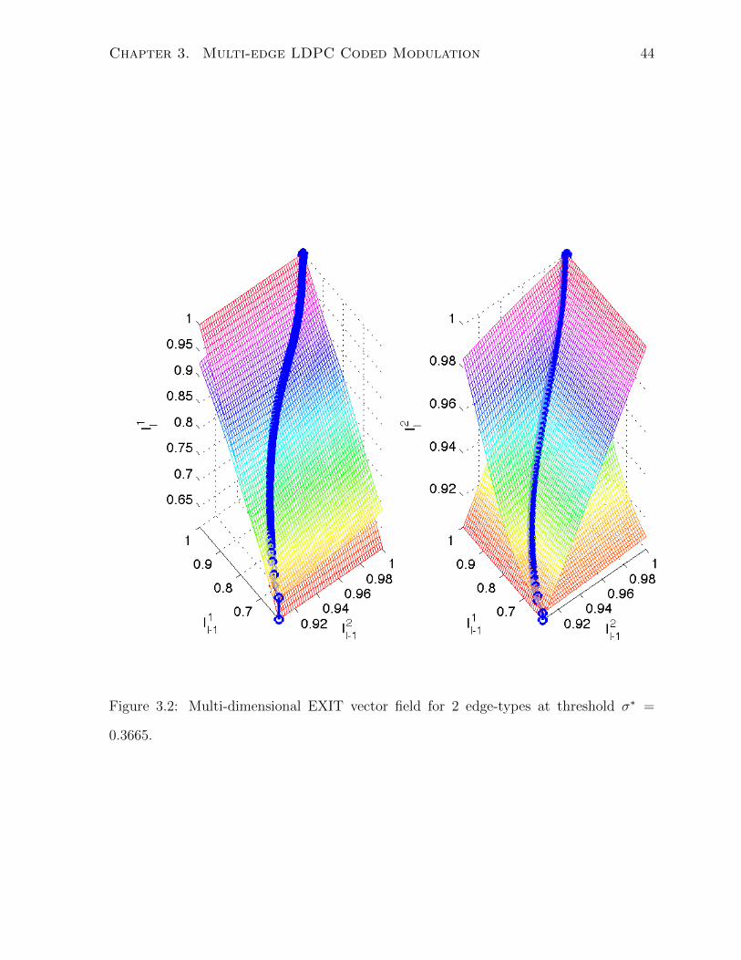
Chapter 3. Multi-edge LDPC Coded Modulation 44
Figure 3.2: Multi-dimensional EXIT vector field for 2 edge-types at threshold σ∗ =
0.3665.
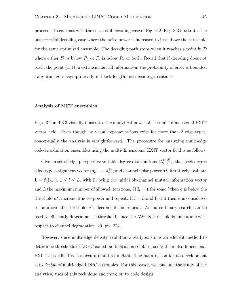
Chapter 3. Multi-edge LDPC Coded Modulation 45
proceed. To contrast with the successful decoding case of Fig. 3.2, Fig. 3.3 illustrates the
unsuccessful decoding case where the noise power is increased to just above the threshold
for the same optimized ensemble. The decoding path stops when it reaches a point in D
where either F1 is below R1 or F2 is below R2 or both. Recall that if decoding does not
reach the point (1, 1) in extrinsic mutual information, the probability of error is bounded
away from zero asymptotically in block-length and decoding iterations.
Analysis of MET ensembles
Figs. 3.2 and 3.3 visually illustrates the analytical power of the multi-dimensional EXIT
vector field. Even though no visual representations exist for more than 2 edge-types,
conceptually the analysis is straightforward. The procedure for analyzing multi-edge
coded modulation ensembles using the multi-dimensional EXIT vector field is as follows.
Given a set of edge-perspective variable degree distributions {λki }dkvi=2, the check degree
edge-type assignment vector (d1c , . . . , dTc ), and channel noise power σ2, iteratively evaluate
Il = f(Il−1), 1 ≤ l ≤ L, with I0 being the initial bit-channel mutual information vector
and L the maximum number of allowed iterations. If Il = 1 for some l then σ is below the
threshold σ∗, increment noise power and repeat. If l = L and Il < 1 then σ is considered
to be above the threshold σ∗, decrement and repeat. An outer binary search can be
used to efficiently determine the threshold, since the AWGN threshold is monotonic with
respect to channel degradation [29, pp. 224].
However, since multi-edge density evolution already exists as an efficient method to
determine thresholds of LDPC coded modulation ensembles, using the multi-dimensional
EXIT vector field is less accurate and redundant. The main reason for its development
is to design of multi-edge LDPC ensembles. For this reason we conclude the study of the
analytical uses of this technique and move on to code design.
Chapter 3. Multi-edge LDPC Coded Modulation 46
Figure 3.3: Multi-dimensional EXIT vector field for 2 edge-types at above threshold
σ = 0.3666.
Chapter 3. Multi-edge LDPC Coded Modulation 47
3.2.2 Design of multi-edge coded modulation
Code design using the multi-dimensional EXIT vector field is very similar to single-edge
EXIT design in all but one aspect. This is not surprising since the single-edge EXIT
chart is the special 1-dimensional instance of the multi-dimensional EXIT vector field.
The goal remains to optimize the code rate over variable node degree distributions, now
one distribution per edge-type. The solution must satisfy linear constraints on socket
count (2.22) and bit-channel ratio (2.23). Most importantly, the solution must allow for
successful decoding from the initial variable mutual information vector I0 to the point
1. It is this final convergence condition that differs between single-edge and multi-edge
EXIT design. Once we find the equivalent multi-edge convergence condition, the rest of
the optimization problem can be extended from single-edge EXIT charts.
The single-edge convergence condition (2.18) requires the variable node mutual in-
formation to increase at every point in the 1-dimensional domain D after one iteration
of variable and check node updates. This is a sufficient condition in 1-dimension since
the EXIT decoding path is also 1-dimensional. In multi-dimensional EXIT vector fields,
while the decoding path remains 1-dimensional, the domain D is not. A convergence
condition requiring improvement in all edge-type mutual informations such as
f v,k(f c,k(I), Ik0 ) > Ik, ∀I ∈ D (3.14)
is unnecessarily stringent. In the successful decoding example of Fig. 3.2, the EXIT
surface F1 is not above R1 for all of the domain D. The condition is only true in the
projection of the decoding path onto D, which is 1-dimensional. Looking along this
projected path, the EXIT vector field is again a 1-dimensional EXIT chart. This exam-
ple illustrates the difficulty in developing a convergence condition for multi-dimensional
EXIT vector fields. The decoding path changes with optimization parameters, so we do
not know which points in D belong to its projection. However, to impose the convergence
constraint (3.14) we must know the projected path. We solve this problem by taking a
Chapter 3. Multi-edge LDPC Coded Modulation 48
completely different view of the multi-dimensional EXIT vector field, focusing on the
fixed points of the iterated system.
Fixed points of multi-dimensional EXIT vector fields
A fixed point of the multi-dimensional EXIT vector field f is defined to be a point I∗ ∈ D
that satisfies
I∗ = f(I∗). (3.15)
By definition, the point 1 is a fixed point of all multi-dimensional EXIT vector fields.
In the following we provide a sufficient condition for the successful convergence of
multi-dimensional EXIT vector fields. The key to the proof lies in the monotonicity of
f with respect to I. Here we distinguish between two important notations. We make
explicit the dependence of f on bit-channel output mutual information vector I0, and
denote a single vector field update at the point I by fI0(I). We use fI0 to represent the
iterated vector field f ◦· · ·◦ f(I0). The distinguishing idea is that fI0(I) is an actual vector
field evaluation with a vector value, whereas fI0 is only a label.
Lemma 3.1. Let I2 � I1 denote the relation between two mutual information vectors
where Ik2 ≥ Ik1 ∀k ∈ (1, . . . , T ), and I2 � I1 if the components are strictly greater. Then
fI0(I2) � fI0(I1) if I2 � I1.
Proof. Recall the monotonicity property of the functions J(σ2), J−1(I) first used in
the proof of Proposition 3.1. Given this property and non-negativity of variable degree
distributions, the claim is equivalent to showing a stripped down version of the vector
field update equations (3.8)
(dkc − 1)J−1(1− Ik) +T∑t=1t6=k
dtcJ−1(1− I t) (3.16)
Chapter 3. Multi-edge LDPC Coded Modulation 49
monotonically decreases (or remains constant) for I2 � I1. Assume only one component
k′ increases between I2 and I1. Then since mutual information is upper-bounded by
1, J−1(1 − Ik′) decreases. For k = k′, since the minimum useful check degree is 2,
the term containing Ik′
in (3.16) decreases. The same argument applies for the k 6= k′
case. Therefore the claim is true for the increase of only one component of the mutual
information vector.
Since (3.16) is a sum of terms each containing a different component of the input
mutual information vector, the general case where I2 � I1 is true by the superposition
principle.
Now we are ready to prove a sufficient convergence condition for the multi-dimensional
EXIT vector field.
Theorem 3.1. Let D = D \ 1, the multi-dimensional EXIT iterated vector field fI0 will
successfully converge to 1 as l→∞, if it has no fixed points in D.
Proof. Given that fI0 has no fixed points in D and by Proposition 3.1 the vector field
only maps to D, we must have fI0(I0) � I0 otherwise I0 is a fixed point in D. Assuming
this holds for Il−1, for an iterated vector field, Il = fI0(Il−1), hence the assumption
implies Il � Il−1. From the monotonicity Lemma 3.1 we know that if Il � Il−1 then
fI0(Il) � fI0(Il−1). Since there are no fixed points in D and fI0(Il) is upper-bounded by
1, by induction we have fI0 converging to 1 as l→∞.
The backward-difference vector field
Theorem 3.1 suggests that to achieve successful convergence of the multi-dimensional
EXIT vector field, the design algorithm must avoid fixed points of fI0 in D. This can be
achieved in practice by using the backward-difference vector field ∇f defined as
Chapter 3. Multi-edge LDPC Coded Modulation 50
∇f(I) ≡ f(I)− I ≡
∇1f(I) = f v,1(f c,1(I), I10 )− I1
∇2f(I) = f v,2(f c,2(I), I20 )− I2...
......
∇T f(I) = f v,T (f c,T (I), IT0 )− IT
. (3.17)
The reason for using ∇f is straightforward since by definition of a fixed point I∗,
f(I∗) − I∗ = 0 therefore ∇f(I∗) = 0. Alternatively, one can consider the backward-
difference vector field as a difference-based representation of an EXIT decoding path.
Let {I′l} denote an EXIT decoding sequence in D where at the lth iteration, the output
of the EXIT update vector field is I′l. We can write this sequence using elements of ∇f
as
I′l = I0 +l−1∑i=1
∇f(I′i). (3.18)
If there exists i′ such that ∇f(I′i′) = 0 then decoding will not progress beyond I′i′ .
Using the backward-difference vector field, the convergence condition in Theorem 3.1 can
be written as
∇f(I) 6= 0, ∀I ∈ D. (3.19)
Fig. 3.4 shows the backward-difference vector field for the optimized 2 edge-type
Gray-labelled 16-QAM ensemble used in Fig. 3.2. The domain D has been quantized to
a 30 by 30 grid. The decoding path is represented by the black vector field streamline.
The arrows are coloured according to the basin of attraction of the fixed point to which
they belong. In the successful decoding case only the fixed point 1 exists, hence all arrows
are coloured blue to indicate that they belong to its basin of attraction.
To derive the operational convergence constraint to be used in an optimization prob-
lem, first write (3.17) explicitly showing the optimization parameters: the variable degree
distribution coefficients
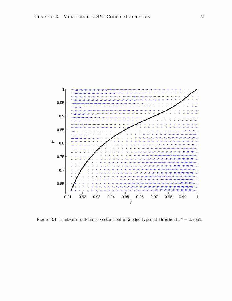
Chapter 3. Multi-edge LDPC Coded Modulation 51
0.91 0.92 0.93 0.94 0.95 0.96 0.97 0.98 0.99 1
0.65
0.7
0.75
0.8
0.85
0.9
0.95
1
I2
I1
Figure 3.4: Backward-difference vector field of 2 edge-types at threshold σ∗ = 0.3665.
Chapter 3. Multi-edge LDPC Coded Modulation 52
f v,k(f c,k(I), Ik0 )− Ik =
dkv∑i=2
λki J[(i− 1)J−1[f c,k(I)] + σ2
k
]− Ik (3.20)
=
dkv∑i=2
λki J[(i− 1)J−1[f c,k(I)] + σ2
k
]− Ik
dkv∑i=2
λki (3.21)
=
dkv∑i=2
λki
(J[(i− 1)J−1[f c,k(I)] + σ2
k
]− Ik
)(3.22)
where (3.21) uses the fact that {λki }dkvi=2 is a probability.
Let gv,ki (f c,k(I), Ik0 ) denote J [(i− 1)J−1[f c,k(I)] + σ2k], we have
f v,k(f c,k(I), Ik0 )− Ik =
dkv∑i=2
λki
(gv,ki (f c,k(I), Ik0 )− Ik
)(3.23)
which is a linear combination of the backward-differences for each variable degree. Define
the elementary backward-difference to be
∇ki f(I) ≡ gv,ki (fc,k(I), Ik0 )− Ik. (3.24)
Finally, we can write ∇f(I) in terms of ∇ki f(I)
∇f(I) =
d1v∑i=2
λ1i∇1i f(I),
d2v∑i=2
λ2i∇2i f(I), . . . ,
dTv∑i=2
λTi ∇Ti f(I)
(3.25)
By using the backward-difference vector field, we recover the elementary EXIT func-
tion representation of the overall EXIT chart first given in (2.19) for single-edge EXIT
charts. Now we can give a practical convergence condition for use in the optimization
problem.
Multi-dimensional EXIT convergence condition
For the multi-dimensional EXIT vector field defined by the specialized multi-edge variable
and check node degree distributions (3.1), (3.3), with fixed maximum variable degrees
Chapter 3. Multi-edge LDPC Coded Modulation 53
dkv , check degree assignment vector (d1c , . . . , dTc ), and bit-channel noise variances σ2
k, a
sufficient condition for the convergence of the EXIT iterated vector field is
‖∇f(I)‖2 > 0, ∀I ∈ D (3.26)
or in expanded form
T∑k=1
dkv∑i=2
λki∇ki f(I)
2
> 0, ∀I ∈ D. (3.27)
Two details must be addressed in practice. The domain D must be quantized to a
finite number of points using some quantization method. We use uniform quantization
with the same resolution in each edge-type. For example a resolution of 30 points was
used in generating Fig. 3.4. Furthermore, the strict inequality in (3.26) cannot be used
as a constraint in optimization. We modify the condition slightly by introducing a small
positive tolerance ε to allow equality
‖∇f(I)‖2 ≥ ε, ∀I ∈ D. (3.28)
The tolerance ε has been observed to be highly dependent on the quantization, max-
imum variable degree dkv , bit-channel noise variance σ2k and to a lesser extent the check
degree assignment vector.
Fig. 3.5 shows the backward-difference vector field for the same optimized ensemble
as Fig. 3.4, except noise power has been increased to above threshold. There are now
two stable fixed points in the domain D at 1 and near the point where the decoding path
terminates. An unstable fixed point lies somewhere between the stable fixed points near
the separation between the red and blue arrows. Again, the arrow colours denote the
basin of attraction of fixed points. Here, the blue arrows belong to the basin of attraction
of the fixed point 1, and the red arrows belong to the basin of attraction of the lower left
fixed point.
Chapter 3. Multi-edge LDPC Coded Modulation 54
In support of the practical convergence condition (3.28), the point marked by the pink
square is where ‖∇f(I)‖2 is at its minimum value. The correspondence between where
the multi-dimensional EXIT vector field stops improving and the estimate given by the
practical convergence condition is clear. A lower resolution was used in Fig. 3.5 for
illustrative purposes. At sufficiently high resolutions, (3.28) is a reliable approximation
of the theoretical convergence condition of Theorem 3.1.
Multi-edge coded modulation optimization
Our parameterization of the multi-edge ensemble for high-order coded modulation uses
variable node-perspective degree distribution (3.1) and check node-perspective degree
distribution (3.3). In Sec. 3.1.1 we concluded that concentrating the check degree to
a single total degree with edge-type assignment vector (d1c , . . . , dTc ) does not degrade
performance significantly over general check degree distributions. Therefore, the check
node edge-type assignment vector is assumed to be given at design time. The AWGN
channel noise power σ2 is also assumed to be fixed at design time. The bit-channel
mutual informations can then be empirically determined. Lastly, the maximum variable
node degrees dkv are chosen at design time.
Under these assumptions, an optimization problem can be setup to optimize the code
rate over the variable node degree distributions{λki }dkvi=2. We derive the constraints in the
following.
Since the optimization parameters {λki }dkvi=2 are normalized edge-perspective variable
degree distributions (2.25), they are constrained to be probabilities
dkv∑i=2
λki = 1 (3.29)
λki ≥ 0 (3.30)
λki ≤ 1. (3.31)
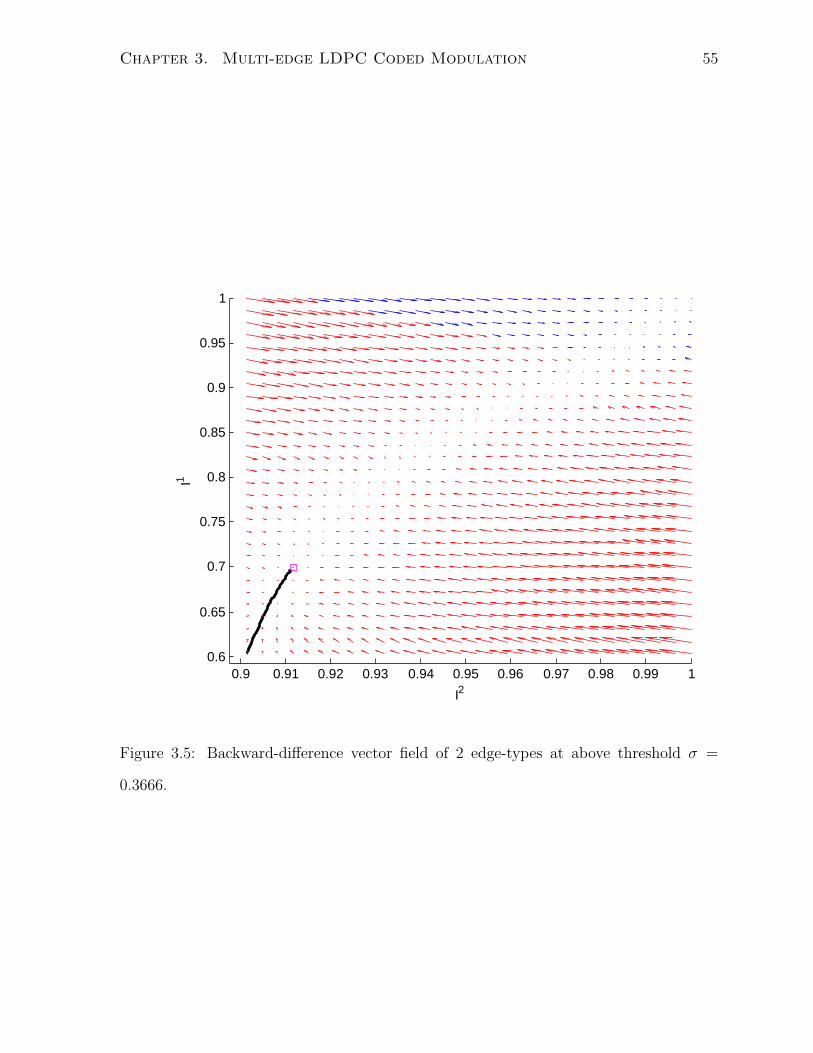
Chapter 3. Multi-edge LDPC Coded Modulation 55
0.9 0.91 0.92 0.93 0.94 0.95 0.96 0.97 0.98 0.99 10.6
0.65
0.7
0.75
0.8
0.85
0.9
0.95
1
I2
I1
Figure 3.5: Backward-difference vector field of 2 edge-types at above threshold σ =
0.3666.
Chapter 3. Multi-edge LDPC Coded Modulation 56
Recall from Sec. 2.3 that all multi-edge degree distribution pairs (L(x, r), R(x)) must
satisfy the socket-count (2.22) and the channel-ratio (2.23) constraints. A slight compli-
cation occurs due to the constraints being stated in node-perspective degree distributions
while the optimization parameters are edge-perspective degree distributions. Assuming
(3.29) holds, there exists a conversion between the coefficients of the two degree distri-
butions
Li,k =1
T
λki /i∑i λ
ki /i
. (3.32)
The reader may verify the conversion by plugging in (3.32) into (2.25). The 1/T
factor is used to satisfy the channel-ratio constraint as explained below.
From the socket-count constraint, on the variable side
∂xkL(1,1) =∑i
iLi,k
=∑i
i1
T
λki /i∑j λ
kj/j
=∑i
λkiT∑
j λkj/j
=1
T∑
j λkj/j
(3.33)
where the last step assumes (3.29) is satisfied. On the check side
∂xkR(1) = dkcR (3.34)
together they form the constraint on edge-type k
1
Tdkc∑
j λkj/j
= R. (3.35)
For T different edge-types, there are T different expressions each containing {λki }dkvi=2
Chapter 3. Multi-edge LDPC Coded Modulation 57
which all equal R. After cancelling T and simple algebraic manipulations, the socket-
count constraint produces(T2
)linear constraints
d1c∑
iλ1ii
= d2c∑
iλ2ii
d1c∑
iλ1ii
= d3c∑
iλ3ii
......
...
d1c∑
iλ1ii
= dTc∑
iλTii
d2c∑
iλ2ii
= d3c∑
iλ3ii
......
...
dT−1c
∑iλT−1i
i= dTc
∑iλTii.
(3.36)
The channel-ratio constraint is satisfied by the inclusion of the factor 1/T
∂rkL(1,1) =∑i
Li,k
=∑i
1
T
λki /i∑j λ
kj/j
=1
T
∑i λ
ki /i∑
j λkj/j
=1
T(3.37)
and does not impose additional constraints on the optimization problem.
Lastly, we have the inequality convergence constraint (3.28) at every point of a quan-
tized version of D. Note that it is quadratic in {λki }dkvi=2.
For T edge-types, there are a total of T linear equality constraints from (3.29),(T2
)linear equality constraints from (3.36), 2T linear inequality constraints from (3.30) and
(3.31), and most importantly quadratic inequality constraints (3.28), the number of which
depends on the quantization resolution of D.
The code rate objective function is linear in {λki }dkvi=2
Chapter 3. Multi-edge LDPC Coded Modulation 58
maxλki
{L(1,1)−R(1)} = maxλki
{∑k
∑i
1
T
λki /i∑j λ
kj/j−R
}
= maxλki
{∑k
1
T− 1
Td1c∑
i λ1i /i
}
= maxλki
{1− 1
Td1c∑
i λ1i /i
}= min
λki
{1
Td1c∑
i λ1i /i
}= max
λki
{∑i
λ1i /i
}. (3.38)
The variable degree distribution for edge-type 1 was arbitrarily used to derive (3.38),
any edge-type will suffice since they were all constrained to R by (3.36).
In summary, the multi-edge LDPC coded modulation optimization problem consists of
maximizing (3.38) over parameters {λki }dkvi=2 subject to linear constraints (3.29),(3.30),(3.31),
(3.36), and quadratic constraint (3.28). We call this optimization problem the multi-edge
LDPC coded modulation optimization (ME-LCM-OPT).
Higher-order extension
For high-order modulation with T distinct bit-channels, solving ME-LCM-OPT for T
sets of variable degree distributions {λki }dkvi=2 is a valid design method. An easier method,
however, is to exploit the nested structure inherent in coded modulation. For example, in
the decomposition of the symbol channel into bit-channels in MLC, upper bit-channels
depended on lower bit-channels. We will leverage this characteristic to simplify code
design for high-order modulation where the number of edge-types is large.
Moreover, in implementation it is often desirable to use a single code at the transmit-
ter and receiver which can quickly adapt to different code rates and constellation sizes
according to varying channel conditions. Solving ME-LCM-OPT for a rate 3/4 16-QAM
code and rate 5/6 64-QAM code is likely to result in two completely different codes.
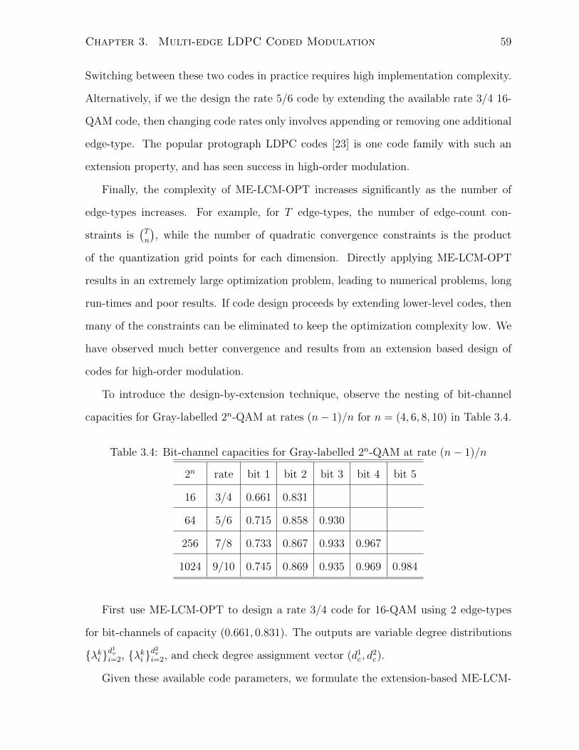
Chapter 3. Multi-edge LDPC Coded Modulation 59
Switching between these two codes in practice requires high implementation complexity.
Alternatively, if we the design the rate 5/6 code by extending the available rate 3/4 16-
QAM code, then changing code rates only involves appending or removing one additional
edge-type. The popular protograph LDPC codes [23] is one code family with such an
extension property, and has seen success in high-order modulation.
Finally, the complexity of ME-LCM-OPT increases significantly as the number of
edge-types increases. For example, for T edge-types, the number of edge-count con-
straints is(Tn
), while the number of quadratic convergence constraints is the product
of the quantization grid points for each dimension. Directly applying ME-LCM-OPT
results in an extremely large optimization problem, leading to numerical problems, long
run-times and poor results. If code design proceeds by extending lower-level codes, then
many of the constraints can be eliminated to keep the optimization complexity low. We
have observed much better convergence and results from an extension based design of
codes for high-order modulation.
To introduce the design-by-extension technique, observe the nesting of bit-channel
capacities for Gray-labelled 2n-QAM at rates (n− 1)/n for n = (4, 6, 8, 10) in Table 3.4.
Table 3.4: Bit-channel capacities for Gray-labelled 2n-QAM at rate (n− 1)/n
2n rate bit 1 bit 2 bit 3 bit 4 bit 5
16 3/4 0.661 0.831
64 5/6 0.715 0.858 0.930
256 7/8 0.733 0.867 0.933 0.967
1024 9/10 0.745 0.869 0.935 0.969 0.984
First use ME-LCM-OPT to design a rate 3/4 code for 16-QAM using 2 edge-types
for bit-channels of capacity (0.661, 0.831). The outputs are variable degree distributions
{λki }d1vi=2, {λki }
d2vi=2, and check degree assignment vector (d1c , d
2c).
Given these available code parameters, we formulate the extension-based ME-LCM-
Chapter 3. Multi-edge LDPC Coded Modulation 60
OPT by eliminating all constraints involving only λ1i or λ2i . In addition, ∇1f(I) and
∇2f(I) are now fully determined thus simplifying constraint (3.28). With these mod-
ifications, for rate 5/6, 64-QAM code design, the extension-based ME-LCM-OPT now
optimizes the code rate over {λ3i }d3vi=2 only.
Extension-based ME-LCM-OPT also resolves the issue of choosing the check degree
assignment vector when many edge-types are present. If full ME-LCM-OPT is used to
design for 3 edge-types the number of potential check degree assignment vectors for a
total check degree of dc is very large. By extending the available 16-QAM check node
assignment, the only free variable for 64-QAM code design is d3c . In a few attempts the
designer can find the best value and proceed with the optimization.
The extension to 256 and 1024-QAM follows in the same manner. At each extension
step, a new component is appended to the check degree assignment vector, while the
variable degree distribution adds a new set of nodes belonging to the highest bit-level.
Chapter 4
Results
The results of multi-edge LDPC ensembles optimized for high-order coded modulation
are presented. Sec. 4.1 provides the optimized variable degree distributions and check
node assignment vectors with their resulting ensemble thresholds. Sec. 4.2 provides
the probability of error performance of finite block-length realizations of these degree
distributions over the complex AWGN noise channel. Comparisons in both threshold
and finite-length performance are made with state-of-the-art designs whenever data is
available. The performance of our code designs match best reported results, with much
lower design and implementation complexity.
4.1 Threshold
We designed code ensembles for Gray-labelled 2n-QAM at rate (n − 1)/n where n =
(4, 6, 8, 10). The results were found by solving ME-LCM-OPT with high-order extension
using the fmincon solver in MATLAB. The resolution used to quantize D is 50 points
per dimension. The quadratic convergence constraint tolerance used in 16-QAM was
ε = 2.0 × 10⁻⁶, while in 64-QAM and higher the tolerance was ε = 4.3 × 10⁻⁶. The
maximum variable degree for all edge-types is 15. The check degree edge-type assignment
vector for 16-QAM was empirically found to be optimal at (d1c , d2c) = (9, 8). Higher-order
61
Chapter 4. Results 62
components of the assignment vector such as d3c were found by hand in a reduced search
space due to the extension procedure.
The ensemble parameters and thresholds are shown in Table 4.1. The thresholds were
evaluated using discrete density evolution [15] modified for multi-edge-type ensembles.
The “Gap (dB)” in Table. 4.1 is the gap to capacity of the ensemble threshold. Recall
from Sec. 2.1.2 that the capacity of the system under study is not the ultimate Shannon
limit of the channel. It is the capacity after constraining the channel input to a finite
constellation with Gray-labelling and uniform input distribution.
4.1.1 Discussion
At a maximum variable degree of 15, the threshold of the optimal rate 1/2 BICM ensemble
in [22] for 4-PAM has a gap to capacity of 0.199 dB. Since 16-QAM is two independent
4-PAM constellations and there is no published threshold for rate 3/4 16-QAM, we shall
use this gap to capacity as reference. In comparison, the threshold of ME-LCM-OPT
designed rate 3/4 16-QAM code ensemble is as close to capacity as the best available
code. No reference exists for other code rates or higher-order modulations. However,
note that the 64 to 1024 QAM ensemble thresholds are all within 0.214 dB of capacity,
likely constrained by the choice of maximum variable degree.
The main goal of the ME-LCM-OPT design method is to match variable node degrees
with the level of error protection required by each distinct high-order modulation bit-
channel. In Table. 4.1 the bolded entries mark the most significant degree distribution
weights for each bit-level. Recall that bit-channel quality increases from level 1 thru 5
according to Table 3.4. At the lowest quality bit-channel 1, degree distribution {λ1i }d1vi=2
contains significant weight at degree 15 variable nodes which provide the best error
protection, while balancing out their low rates by using degree 2 and 3 variable nodes.
At bit-level 2 where the bit-channel capacity at 0.831 is significantly higher than bit-level
1, the resultant {λ2i }d2vi=2 moves away from the strong error correction of degree 15 variable
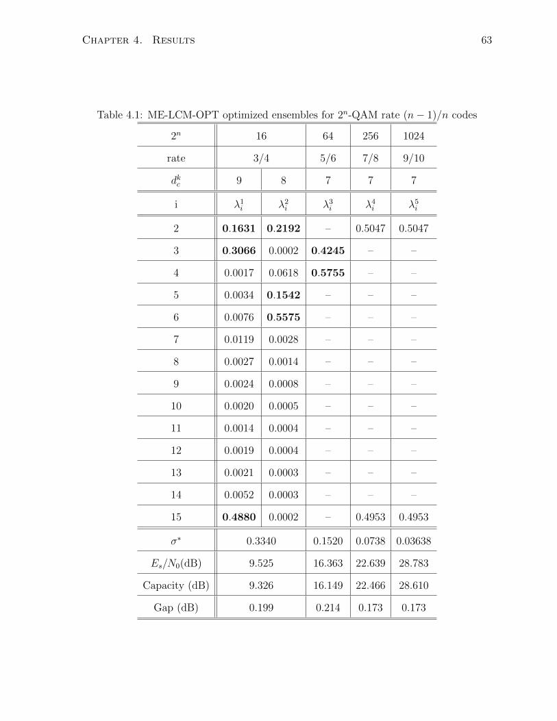
Chapter 4. Results 63
Table 4.1: ME-LCM-OPT optimized ensembles for 2n-QAM rate (n− 1)/n codes
2n 16 64 256 1024
rate 3/4 5/6 7/8 9/10
dkc 9 8 7 7 7
i λ1i λ2i λ3i λ4i λ5i
2 0.1631 0.2192 – 0.5047 0.5047
3 0.3066 0.0002 0.4245 – –
4 0.0017 0.0618 0.5755 – –
5 0.0034 0.1542 – – –
6 0.0076 0.5575 – – –
7 0.0119 0.0028 – – –
8 0.0027 0.0014 – – –
9 0.0024 0.0008 – – –
10 0.0020 0.0005 – – –
11 0.0014 0.0004 – – –
12 0.0019 0.0004 – – –
13 0.0021 0.0003 – – –
14 0.0052 0.0003 – – –
15 0.4880 0.0002 – 0.4953 0.4953
σ∗ 0.3340 0.1520 0.0738 0.03638
Es/N0(dB) 9.525 16.363 22.639 28.783
Capacity (dB) 9.326 16.149 22.466 28.610
Gap (dB) 0.199 0.214 0.173 0.173
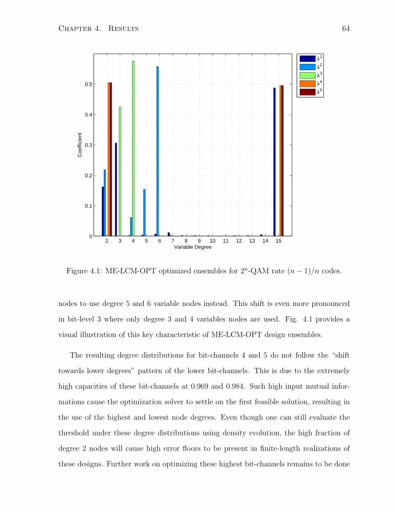
Chapter 4. Results 64
2 3 4 5 6 7 8 9 10 11 12 13 14 150
0.1
0.2
0.3
0.4
0.5
Variable Degree
Coe
ffici
ent
λ1
λ2
λ3
λ4
λ5
Figure 4.1: ME-LCM-OPT optimized ensembles for 2n-QAM rate (n− 1)/n codes.
nodes to use degree 5 and 6 variable nodes instead. This shift is even more pronounced
in bit-level 3 where only degree 3 and 4 variables nodes are used. Fig. 4.1 provides a
visual illustration of this key characteristic of ME-LCM-OPT design ensembles.
The resulting degree distributions for bit-channels 4 and 5 do not follow the “shift
towards lower degrees” pattern of the lower bit-channels. This is due to the extremely
high capacities of these bit-channels at 0.969 and 0.984. Such high input mutual infor-
mations cause the optimization solver to settle on the first feasible solution, resulting in
the use of the highest and lowest node degrees. Even though one can still evaluate the
threshold under these degree distributions using density evolution, the high fraction of
degree 2 nodes will cause high error floors to be present in finite-length realizations of
these designs. Further work on optimizing these highest bit-channels remains to be done
Chapter 4. Results 65
to make sure the code designs will be practically useful.
4.1.2 High code rate designs
To verify the capability of ME-LCM-OPT to design across code rates, code ensembles
were optimized for Gray-labelled 16-QAM with a maximum variable degree of 15, with
targeted code rates of 1/2, 2/3, 3/4, 5/6, 7/8, and 9/10. Only rates higher than 1/2 were
used because bandwidth-efficient coded modulation only works with high rate codes. The
resulting variable degree distributions and thresholds are given in Tables 4.2 and 4.3.
The mean gap to capacity across all 6 code rates is 0.216 with a maximum gap of
0.236. These values are consistent with the performance reported in [22] for a maximum
variable node of degree 15, and also with the designs in Table 4.1. The difference in
degree distributions between edge-types 1 and 2 remains, as degree 15 is nearly always
used in edge-type 1 and never used in edge-type 2. These results help to confirm the
ME-LCM-OPT technique as an effective method for designing high rate codes used in
LDPC coded modulation.
4.2 Finite-length
For finite-length realization of the code ensembles, in order to obtain good error floors
the parity-check matrices were generated using the improved progressive-edge-growth
(PEG) algorithm [41, 42] modified for multi-edge-type codes. One key modification is
to interleave variable nodes from different edge-types to their proper bit-level positions
according to bit-channel quality, before applying the PEG algorithm. Another modifica-
tion is to impose strict check degree edge counts for all edge-types, whereas check degrees
are allowed to vary in the original PEG algorithm.
Simulations to estimate probability of bit and frame errors were written in C and
compiled using GNU gcc version 4.2.1. The implemented system was shown in Fig. 2.1.
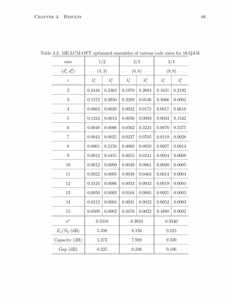
Chapter 4. Results 66
Table 4.2: ME-LCM-OPT optimized ensembles of various code rates for 16-QAM
rate 1/2 2/3 3/4
(d1c , d2c) (4, 3) (6, 6) (9, 8)
i λ1i λ2i λ1i λ2i λ1i λ2i
2 0.2448 0.3362 0.1970 0.2684 0.1631 0.2192
3 0.1572 0.3950 0.3289 0.0536 0.3066 0.0002
4 0.0663 0.0020 0.0022 0.0172 0.0017 0.0618
5 0.1224 0.0013 0.0056 0.0093 0.0034 0.1542
6 0.0048 0.0006 0.0562 0.3224 0.0076 0.5575
7 0.0043 0.0025 0.0237 0.0705 0.0119 0.0028
8 0.0061 0.2150 0.0068 0.0850 0.0027 0.0014
9 0.0012 0.0455 0.0055 0.0241 0.0024 0.0008
10 0.0012 0.0000 0.0049 0.0861 0.0020 0.0005
11 0.0022 0.0005 0.0049 0.0463 0.0014 0.0004
12 0.3124 0.0006 0.0033 0.0043 0.0019 0.0004
13 0.0050 0.0003 0.0104 0.0085 0.0021 0.0003
14 0.0212 0.0004 0.0031 0.0022 0.0052 0.0003
15 0.0509 0.0002 0.3476 0.0022 0.4880 0.0002
σ∗ 0.5310 0.3910 0.3340
Es/N0 (dB) 5.498 8.156 9.525
Capacity (dB) 5.273 7.920 9.339
Gap (dB) 0.225 0.236 0.186
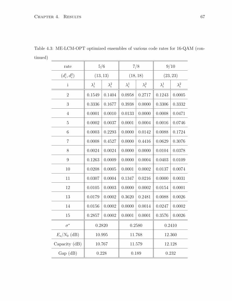
Chapter 4. Results 67
Table 4.3: ME-LCM-OPT optimized ensembles of various code rates for 16-QAM (con-
tinued)
rate 5/6 7/8 9/10
(d1c , d2c) (13, 13) (18, 18) (23, 23)
i λ1i λ2i λ1i λ2i λ1i λ2i
2 0.1549 0.1404 0.0958 0.2717 0.1243 0.0005
3 0.3336 0.1677 0.3938 0.0000 0.3306 0.3332
4 0.0001 0.0010 0.0133 0.0000 0.0008 0.0471
5 0.0002 0.0037 0.0001 0.0004 0.0016 0.0746
6 0.0003 0.2293 0.0000 0.0142 0.0088 0.1724
7 0.0008 0.4527 0.0000 0.4416 0.0629 0.3076
8 0.0024 0.0024 0.0000 0.0000 0.0104 0.0378
9 0.1263 0.0009 0.0000 0.0004 0.0403 0.0109
10 0.0208 0.0005 0.0001 0.0002 0.0137 0.0074
11 0.0307 0.0004 0.1347 0.0216 0.0000 0.0031
12 0.0105 0.0003 0.0000 0.0002 0.0154 0.0001
13 0.0179 0.0002 0.3620 0.2481 0.0088 0.0026
14 0.0156 0.0002 0.0000 0.0014 0.0247 0.0002
15 0.2857 0.0002 0.0001 0.0001 0.3576 0.0026
σ∗ 0.2820 0.2580 0.2410
Es/N0 (dB) 10.995 11.768 12.360
Capacity (dB) 10.767 11.579 12.128
Gap (dB) 0.228 0.189 0.232
Chapter 4. Results 68
IID channel adapters described in Sec. 2.1.1 were included in the simulation. Since the
iid channel adapters result in output symmetric bit-channels, we only transmitted the
all-zeros codeword to estimate the equivalent error performance for all codewords.
4.2.1 Rate 3/4 Gray-labelled 16-QAM
Figs. 4.2, 4.3 and 4.4 show the probability of bit and frame errors (BER, FER) with
respect to the per-bit signal-to-noise ratio Eb/N0 in dB for codeword lengths of 4096 (4K),
8192 (8K) and 16384 (16K) respectively. The code ensemble used is the rate 3/4 16-QAM
code with a threshold of 9.525 dB Es/N0 or 4.754 dB Eb/N0. The ensemble threshold is
indicated by the black vertical line in the figures. The red vertical line indicates capacity.
The coloured dots indicate the ±3σ error bars on the BER and FER curves, with some
of the lower error bars missing due to the logarithmic scale used.
The Eb/N0 axis of the three figures are fixed for comparison. Choosing an arbitrary
point of reference on the BER curve, for example the 10−6 point, we see that the SNRs
required are approximately 5.78 dB, 5.49 dB, and 5.27 dB for 4K, 8K and 16K. The 10−6
SNR for 16K is 0.52 dB from threshold and 0.72 dB from capacity.
The figures show an FER error floor at approximately 10−4. A quick calculation gives
the number of error bits per erroneous frame to be 20, 17 and 10 bits for 4K, 8K and 16K.
An efficient concatenated code solution can reduce the error floor to negligible levels and
has been utilized in the DVB-S2 standard [8]. For example, we can use the (255, 239)
rate 0.937 double error correcting Bose-Chaudhuri-Hocquenghem (BCH) code [43] with
an interleaver that disperses the 10 bit errors among 16384 codeword bits to ensure less
than 2 errors will occur per BCH codeword. If the slight rate loss is not acceptable, then
the inner LDPC code can be designed with the proper rate compensation to obtain the
correct concatenated code rate.
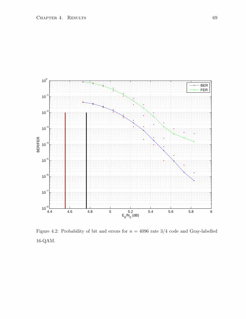
Chapter 4. Results 69
4.4 4.6 4.8 5 5.2 5.4 5.6 5.8 610
−8
10−7
10−6
10−5
10−4
10−3
10−2
10−1
100
Eb/N
0 (dB)
BE
R/F
ER
BERFER
Figure 4.2: Probability of bit and errors for n = 4096 rate 3/4 code and Gray-labelled
16-QAM.

Chapter 4. Results 70
4.4 4.6 4.8 5 5.2 5.4 5.6 5.8 610
−8
10−7
10−6
10−5
10−4
10−3
10−2
10−1
100
Eb/N
0 (dB)
BE
R/F
ER
BERFER
Figure 4.3: Probability of bit and errors for n = 8192 rate 3/4 code and Gray-labelled
16-QAM.
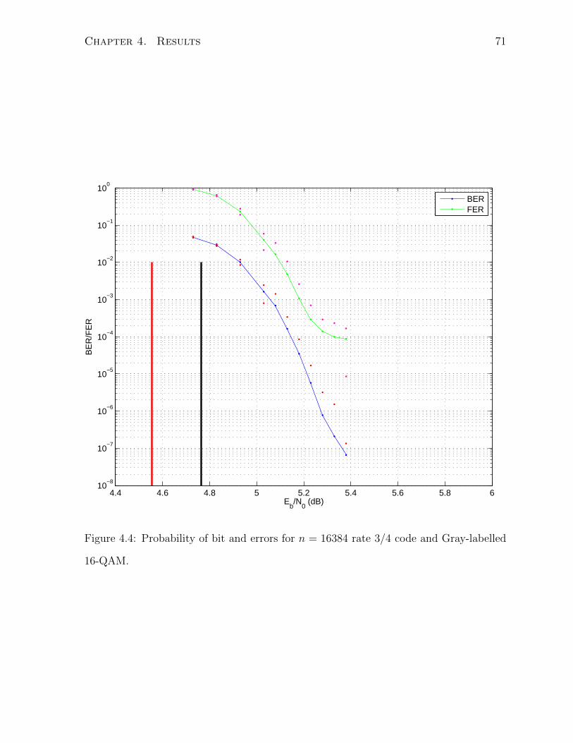
Chapter 4. Results 71
4.4 4.6 4.8 5 5.2 5.4 5.6 5.8 610
−8
10−7
10−6
10−5
10−4
10−3
10−2
10−1
100
Eb/N
0 (dB)
BE
R/F
ER
BERFER
Figure 4.4: Probability of bit and errors for n = 16384 rate 3/4 code and Gray-labelled
16-QAM.
Chapter 4. Results 72
4.2.2 Rate 1/2 Gray-labelled 16-QAM
Fig. 4.5 shows the BER and FER results of the rate 1/2 16-QAM code given in Table
4.2, at a codeword length of 16200 bits. At an BER of 10−6 the code requires an Eb/N0
of 3.27 dB, which is 0.78 dB from threshold and 1.0 dB from capacity. An FER error
floor is present at an FER of 5 × 10⁻⁵. In comparison, as reported in [24], a code with
the same rate and block-length requires an Eb/N0 of 3.17 dB, a difference of 0.1 dB.
Furthermore, the reference [22] code of rate 1/2 at a codeword length of 16200 has the
identical performance as our code [24]. These comparisons indicate that the ME-LCM-
OPT design procedure produces codes that are equivalent to best known codes not only
in terms of threshold, but also in finite-length performance.
4.2.3 Fixed BER performance comparison
For a final summary comparison, we plot the Es/N0 (dB) required by our code designs
to achieve a BER of 10−5 with several published results at the same spectral efficiency.
Efforts were made to select references that provide the fairest possible comparison in
terms of block-length and maximum variable degree. Fig. 4.6(a) plots the Es/N0 required
at a spectral efficiency of 3 bits per channel use for Gray-labelled 16-QAM, while Fig.
4.6(b) shows the comparison at 2 bits per channel use. Blue markers are our ME-LCM-
OPT code designs and the black markers are results from published literature.
Legends for the labelled data points in Fig. 4.6 are given in Table. 4.4. Note that
some descriptions use the number of informations k to define the code, instead of the
overall block-length n.
In Fig. 4.6(a) we compare the n = 4096 (data point 1) and k = 4096 (data point 4)
codes of our design with the AR4JA k = 4096 (data point 5) code. We see that our code
achieves the required BER at the shorter block length of 4096. At the same information
bit length, our code provides a 0.1 dB improvement. Part of this difference is because
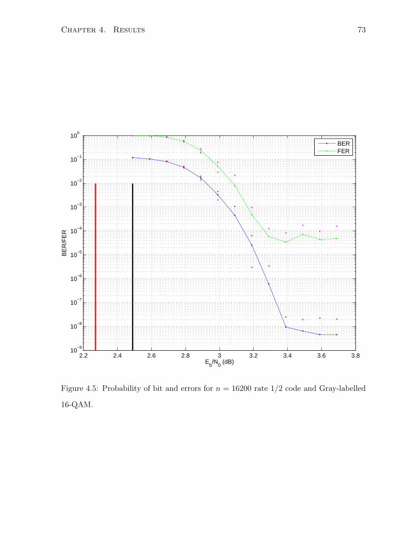
Chapter 4. Results 73
2.2 2.4 2.6 2.8 3 3.2 3.4 3.6 3.810
−9
10−8
10−7
10−6
10−5
10−4
10−3
10−2
10−1
100
Eb/N
0 (dB)
BE
R/F
ER
BERFER
Figure 4.5: Probability of bit and errors for n = 16200 rate 1/2 code and Gray-labelled
16-QAM.
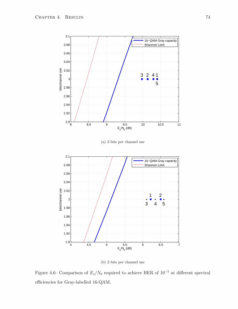
Chapter 4. Results 74
8 8.5 9 9.5 10 10.5 112.9
2.92
2.94
2.96
2.98
3
3.02
3.04
3.06
3.08
3.1
Es/N
0 (dB)
bits
/cha
nnel
use
123 4
5
16−QAM Gray capacityShannon Limit
(a) 3 bits per channel use
4 4.5 5 5.5 6 6.5 71.9
1.92
1.94
1.96
1.98
2
2.02
2.04
2.06
2.08
2.1
Es/N
0 (dB)
bits
/cha
nnel
use
1 2
3 4 5
16−QAM Gray capacityShannon Limit
(b) 2 bits per channel use
Figure 4.6: Comparison of Es/N0 required to achieve BER of 10−5 at different spectral
efficiencies for Gray-labelled 16-QAM.
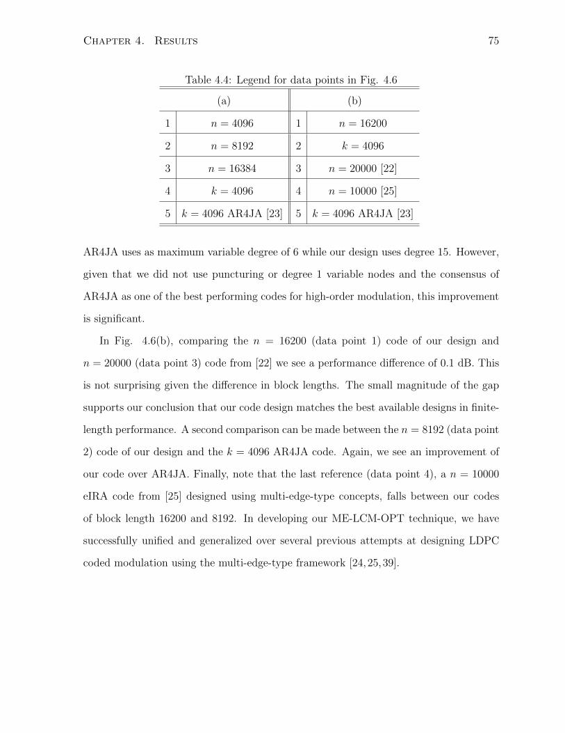
Chapter 4. Results 75
Table 4.4: Legend for data points in Fig. 4.6
(a) (b)
1 n = 4096 1 n = 16200
2 n = 8192 2 k = 4096
3 n = 16384 3 n = 20000 [22]
4 k = 4096 4 n = 10000 [25]
5 k = 4096 AR4JA [23] 5 k = 4096 AR4JA [23]
AR4JA uses as maximum variable degree of 6 while our design uses degree 15. However,
given that we did not use puncturing or degree 1 variable nodes and the consensus of
AR4JA as one of the best performing codes for high-order modulation, this improvement
is significant.
In Fig. 4.6(b), comparing the n = 16200 (data point 1) code of our design and
n = 20000 (data point 3) code from [22] we see a performance difference of 0.1 dB. This
is not surprising given the difference in block lengths. The small magnitude of the gap
supports our conclusion that our code design matches the best available designs in finite-
length performance. A second comparison can be made between the n = 8192 (data point
2) code of our design and the k = 4096 AR4JA code. Again, we see an improvement of
our code over AR4JA. Finally, note that the last reference (data point 4), a n = 10000
eIRA code from [25] designed using multi-edge-type concepts, falls between our codes
of block length 16200 and 8192. In developing our ME-LCM-OPT technique, we have
successfully unified and generalized over several previous attempts at designing LDPC
coded modulation using the multi-edge-type framework [24,25,39].
Chapter 5
Conclusion
In this thesis, we identified a point of improvement to the currently popular LDPC-
BICM scheme for bandwidth-efficient high-order coded modulation. We sought to match
bit-channel quality differences with the inherent differences in error protection in LDPC
codeword bits. A specific multi-edge-type parameterization was developed in order to
impose structure to reduce design complexity while retaining the key property of incor-
porating different bit-channel output densities into the code ensemble.
A new analysis technique using the multi-dimensional EXIT vector field was devel-
oped as an efficient and accurate way of determining the threshold of the multi-edge
parameterization for coded modulation. In order to apply the technique to code design,
a new decoding convergence condition was derived. Using the convergence condition,
the ME-LCM-OPT problem was setup in order to optimize the code ensembles for the
highest code rate at a given channel noise power. We designed several code ensembles
for 16 to 1024 QAM at different code rates, with thresholds as close to capacity as best
available results. Finite-length probability of error performance also matched current
best, with lower design and implementation complexity.
In conclusion, this thesis provided one of the first methods of LDPC code design
for high-order modulation without decomposing the symbol channel into individual bit-
76
Chapter 5. Conclusion 77
channels. In the process, an innovative analysis and design technique for multi-edge-type
ensembles based on EXIT functions was developed, which was shown to be efficient and
accurate when compared to density evolution.
We believe that the multi-edge EXIT-based optimization technique is not limited to
high-order modulation code design, but can also be applied to any application where a
single LDPC code is desired for several different channel output densities. Seeking out
such applications and applying the technique to code design is one of the major topics
of future work. Another possible direction is to extend the optimization procedure to a
variable-check iterative optimization process. While one of the two degree distributions
is being optimized, the other is assumed to be fixed. The roles are reversed in the next
optimization iteration. In doing so, the concentration to a single check degree edge-type
assignment used in this thesis may be relaxed, perhaps with improved results. Lastly,
the well known protograph-based coded modulation scheme using AR4JA protograph
codes [23] has shown excellent performance likely due to the presence of punctured and
degree 1 variable nodes. Future work to include both into the code ensemble may also
provide performance gains.
Bibliography
[1] G. Ungerboeck, “Channel coding with multilevel/phase signals,” IEEE Trans. Inf.
Theory, vol. 28, no. 1, pp. 55 – 67, Jan. 1982.
[2] ——, “Trellis-coded modulation with redundant signal sets Part I: Introduction,”
IEEE Commun. Mag., vol. 25, no. 2, pp. 5–11, Feb. 1987.
[3] C. Berrou, A. Glavieux, and P. Thitimajshima, “Near Shannon limit error-correcting
coding and decoding: Turbo-codes,” in IEEE International Conf. on Comm., vol. 2,
Geneva, Switzerland, May 1993, pp. 1064–1070.
[4] R. Gallager, “Low-density parity-check codes,” IRE Trans. Inf. Theory, vol. 8, no. 1,
pp. 21–28, Jan. 1962.
[5] G. Caire, G. Taricco, and E. Biglieri, “Bit-interleaved coded modulation,” IEEE
Trans. Inf. Theory, vol. 44, no. 3, pp. 927–946, May 1998.
[6] H. Imai and S. Hirakawa, “A new multilevel coding method using error-correcting
codes,” IEEE Trans. Inf. Theory, vol. 23, no. 3, pp. 371–377, May 1977.
[7] U. Wachsmann, R. Fischer, and J. B. Huber, “Multilevel codes: theoretical concepts
and practical design rules,” IEEE Trans. Inf. Theory, vol. 45, no. 5, pp. 1361–1391,
Jul. 1999.
[8] Digital Video Broadcasting (DVB); Second generation framing structure, channel
coding and modulation systems for broadcasting, interactive services, news gathering
78
Bibliography 79
and other broadband satellite applications, European Telecommunications Standards
Institute Std., Aug. 2009.
[9] Digital Video Broadcasting (DVB); Frame structure channel coding and modulation
for a second generation digital transmission system for cable systems, European
Telecommunications Standards Institute Std., Jun. 2010.
[10] IEEE Standard for local and metropolitan area networks, Part 16: Air interface for
broadband wireless access systems, Institute of Electrical and Electronic Engineers
Std., May 2009.
[11] Low density parity check codes for use in near-earth and deep space applications,
The Consultive Commitee for Space Data Systems Std., Sep. 2007.
[12] H. Jin, A. Khandekar, and R. McEliece, “Irregular repeat-accumulate codes,” in
Proc. 2nd Int. Symp. Turbo Codes Related Topics, Brest, France, Sep. 2000.
[13] R. Tanner, “A recursive approach to low complexity codes,” IEEE Trans. Inf. The-
ory, vol. 27, no. 5, pp. 533 – 547, Sep. 1981.
[14] T. J. Richardson, M. A. Shokrollahi, and R. L. Urbanke, “Design of capacity-
approaching irregular low-density parity-check codes,” IEEE Trans. Inf. Theory,
vol. 47, no. 2, pp. 619–637, Feb. 2001.
[15] S.-Y. Chung, G. D. Forney, Jr., T. J. Richardson, and R. L. Urbanke, “On the
design of low-density parity-check codes within 0.0045 dB of the Shannon limit,”
IEEE Commun. Lett., vol. 5, no. 2, pp. 58–60, Feb. 2001.
[16] F. Kschischang, B. Frey, and H.-A. Loeliger, “Factor graphs and the sum-product
algorithm,” IEEE Trans. Inf. Theory, vol. 47, no. 2, pp. 498–519, Feb. 2001.
Bibliography 80
[17] M. Luby, M. Mitzenmacher, M. Shokrollahi, and D. Spielman, “Improved low-
density parity-check codes using irregular graphs,” IEEE Trans. Inf. Theory, vol. 47,
no. 2, pp. 585–598, Feb. 2001.
[18] T. Richardson and R. Urbanke, “The capacity of low-density parity-check codes
under message-passing decoding,” IEEE Trans. Inf. Theory, vol. 47, no. 2, pp. 599–
618, Feb. 2001.
[19] Y. Li and W. E. Ryan, “Bit-reliability mapping in LDPC-coded modulation sys-
tems,” IEEE Commun. Lett., vol. 9, no. 1, pp. 1–3, Jan. 2005.
[20] R. Maddock and A. Banihashemi, “Reliability-based coded modulation with low-
density parity-check codes,” IEEE Trans. Commun., vol. 54, no. 3, pp. 403–406,
Mar. 2006.
[21] J. Lei and W. Gao, “Matching graph connectivity of LDPC codes to high-order mod-
ulation by bit interleaving,” in 46th Annual Allerton Conference on Communication,
Control and Computing, Sep. 2008, pp. 1059–1064.
[22] J. Hou, P. H. Siegel, L. B. Milstein, and H. D. Pfister, “Capacity-approaching
bandwidth-efficient coded modulation schemes based on low-density parity-check
codes,” IEEE Trans. Inf. Theory, vol. 49, no. 9, pp. 2141–2155, Sep. 2003.
[23] D. Divsalar and C. Jones, “Protograph based low error floor LDPC coded mod-
ulation,” in IEEE Mil. Comm. Conf., Atlantic City, New Jersey, Oct. 2005, pp.
378–385.
[24] H. Sankar, N. Sindhushayana, and K. R. Narayanan, “Design of low-density parity
check LDPC codes for high order constellations,” in IEEE Global Telecom. Conf.,
vol. 5, Nov. 2004, pp. 3113–3117.
Bibliography 81
[25] G. Durisi, L. Dinoi, and S. Benedetto, “eIRA codes for coded modulation systems,”
in IEEE International Conf. on Comm., vol. 3, Istanbul, Turkey, Jun. 2006, pp.
1125–1130.
[26] S. Sandberg and N. Von Deetzen, “Design of bandwidth-efficient unequal error pro-
tection LDPC codes,” IEEE Trans. Commun., vol. 58, no. 3, pp. 802–811, Mar.
2010.
[27] L. Yan and W. E. Ryan, “Design of LDPC-coded modulation schemes,” un-
published. [Online]. Available: http://www2.engr.arizona.edu/∼ryan/publications/
turbo-symp-03.pdf
[28] M. Ardakani, T. Esmailian, and F. R. Kschischang, “Near-capacity coding in multi-
carrier modulation systems,” IEEE Trans. Commun., vol. 52, no. 11, pp. 1880–1889,
Nov. 2004.
[29] T. Richardson and R. Urbanke, Modern Coding Theory. Cambridge University
Press, 2008.
[30] G. D. Forney, Jr., “Trellis shaping,” IEEE Trans. Inf. Theory, vol. 38, no. 2, pp.
281–300, Mar. 1992.
[31] F. R. Kschischang and S. Pasupathy, “Optimal nonuniform signaling for Gaussian
channels,” IEEE Trans. Inf. Theory, vol. 39, no. 3, pp. 913–929, Mar. 1993.
[32] R. Storn and K. Price, “Differential evolution, a simple and efficient heuristic for
global optimization over continuous spaces,” Journal of Global Optimization, vol. 11,
pp. 341–359, 1997.
[33] A. Papoulis and S. U. Pillai, Probability, random variables and stochastic processes,
4th ed. McGraw-Hill Higher Education, 2002.
Bibliography 82
[34] S. Y. Chung, T. Richardson, and R. Urbanke, “Analysis of sum-product decoding of
low-density parity-check codes using a Gaussian approximation,” IEEE Trans. Inf.
Theory, vol. 47, no. 2, pp. 657–670, Feb. 2001.
[35] M. Ardakani and F. R. Kschischang, “A more accurate one-dimensional analysis and
design of irregular LDPC codes,” IEEE Trans. Commun., vol. 52, no. 12, pp. 2106
– 2114, Dec. 2004.
[36] S. ten Brink, G. Kramer, and A. Ashikhmin, “Design of low-density parity-check
codes for modulation and detection,” IEEE Trans. Commun., vol. 52, no. 4, pp.
670–678, Apr. 2004.
[37] A. Ashikhmin, G. Kramer, and S. ten Brink, “Extrinsic information transfer func-
tions: model and erasure channel properties,” IEEE Trans. Inf. Theory, vol. 50,
no. 11, pp. 2657–2673, Nov. 2004.
[38] E. W. Weisstein. (2011, May) Partition function P. MathWorld - A Wolfram Web
Resource. [Online]. Available: http://mathworld.wolfram.com/PartitionFunctionP.
html
[39] H. V. Neto, W. Henkel, and V. C. da Rocha, Jr., “Multi-edge type unequal error
protection LDPC codes,” Jan. 2011, unpublished. ArXiv:1101.5985v1. [Online].
Available: http://arxiv.org/abs/1101.5985v1
[40] S. ten Brink, “Convergence behaviour of iteratively decoded parallel concatenated
codes,” IEEE Trans. Commun., vol. 49, no. 10, pp. 1727–1737, Oct. 2001.
[41] H. Xiao and A. H. Banihashemi, “Improved progressive-edge-growth (PEG) con-
struction of irregular LDPC codes,” Communications Letters, IEEE, vol. 8, no. 12,
pp. 715 – 717, Dec. 2004.
Bibliography 83
[42] X. Y. Hu, E. Eleftheriou, and D. M. Arnold, “Regular and irregular progressive
edge-growth Tanner graphs,” IEEE Trans. Inf. Theory, vol. 51, no. 1, pp. 386–398,
Jan. 2005.
[43] J. Proakis and M. Salehi, Digital Communications, 5th ed. McGraw-Hill Sci-
ence/Engineering/Math, 2007.


![Trellis-Coded Modulation [TCM]](https://img.pdfslide.net/doc/110x75/618ad19974abd138231352ca/trellis-coded-modulation-tcm.jpg)