Embed Size (px)
Citation preview
arX
iv:1
506.
0884
7v1
[q-
fin.
ST]
17
May
201
5
Multifractal characterization of gold market: a
multifractal detrended fluctuation analysis
Provash Mali∗and Amitabha MukhopadhyayDepartment of Physics, University of North Bengal,
West Bengal, Darjeeling 734013, India
Abstract
The multifractal detrended fluctuation analysis technique is employed to ana-lyze the time series of gold consumer price index (CPI) and the market trendof three world’s highest gold consuming countries, namely China, India andTurkey for the period: 1993July 2013. Various multifractal variables, such asthe generalized Hurst exponent, the multifractal exponent and the singularityspectrum, are calculated and the results are fitted to the generalized binomialmultifractal (GBM) series that consists of only two parameters. Special empha-sis is given to identify the possible source(s) of multifractality in these series.Our analysis shows that the CPI series and all three market series are of multi-fractal nature. The origin of multifractality for the CPI time series and Indianmarket series is found due to a long-range time correlation, whereas it is mostlydue to the fat-tailed probability distributions of the values for the Chinese andTurkey markets. The GBM model series more or less describes all the timeseries analyzed here.
PACS numbers: 05.45.Tp; 61.43.-j; 89.65.GhKeywords: Multifractality; Detrended fluctuation analysis; Consumer price index;Long-range time correlation; Generalized binomial multifractal model
1 Introduction
In general, a fractal is a rough or fragmented geometrical shape that can be subdi-vided into parts, each of which is (at least approximately) a reduced-size copy of thewhole. A fractal system is usually described by a scale invariant parameter calledfractal dimension [1]. Many fractals arising in nature have a far more complex scalingrelation than simple fractals and require a set of parameters to specify such objectsthat are known as multifractals. Several approaches have so far been developed andapplied to explore the of fractal properties. For instance, the rescaled adjusted rangeanalysis method was introduced by Hurst [2, 3] (see also [4]), which he himself appliedthe method to his hydrological study. Due to the difficulty of the rescaled analysisin capturing long-range correlations of nonstationary series, Peng et al. [5] proposedan alternative approach to analyze the DNA sequences which is known as detrended
∗E-mail: [email protected]
1
fluctuation analysis (DFA). Although the DFA method is widely used to determinemonofractal scaling properties, it cannot properly describe multi-scale and fractal sub-sets of time series data. One of the simplest type of multifractal analysis has beendeveloped based on the standard partition function multifractal formalism [4, 6]. Thisis a highly successful method for the multifractal characterization of normalized andstationary measures, but it does not give the correct result for nonstationary time se-ries. Based on a generalization of the DFA method, Kantelhardt et al. [7] introducedthe multifractal detrended fluctuation analysis (MF-DFA) for the multifractal charac-terization of nonstationary time series. As a remarkable powerful technique, MF-DFAhas so far been applied to various fields of stochastic analysis, for instance, in mar-kets return analysis [8, 9, 10, 11, 12, 13, 14, 15], in geophysics [16, 17, 20, 18, 19], inbiophysics [21, 22, 23, 24], and also in various branches of basics and applied physics[25, 26, 27, 28, 29, 30].
The study of financial time series has been the focus of intense research by thephysics community in the last several years. Nowadays, there are some excellentcompilations available on this subject, e.g. [31, 32, 33], just to cite some of them. Theprime objective of this kind of analysis is to characterize the statistical properties ofthe time series with the hope that a better understanding of the underlying dynamicscould provide useful information to create new models. Moreover, such knowledgemight be crucial to tackle relevant problems in finance, such as risk management orthe design of optimal portfolios. Henceforth our discussion will be restricted to thetime series analysis of gold market in China, Indian, Turkey and the global consumerprice index (CPI)1.
Gold being one of the most precious metals is always considered as the safestinvestment. Presently the fluctuations of gold market seem quite confusing even tothe regular traders, and it becomes almost impossible to predict its accurate rise orfall. As we know, over the last 2/3 years gold price increases so rapidly that thegold price nowadays is approximately double of the average rate of 2010. The marketgains its highest value of about 1900 USD/ounce in the year 2011, and the recentvalue is about 1300 USD/ounce. Moreover, the day-to-day variation of the market isalso quite remarkable during the last few years. It is now believed that gold is nota commodity anymore, rather a currency which always maintain an inverse relationwith the US economy. So it is quite possible that a part of the change in gold priceis really just a reflection of a change in the value of the US dollar. Sometimes suchchange is insignificant and often the opposite is true. Whatever may be the reason,the dynamical nature of the gold market is quite complex, and one needs to studythe time series of gold price from all possible directions in order to understand theunderlying mechanism.
In this article we apply the MF-DFA technique to characterize the time series ofthe gold CPI and the gold market in China, India and Turkey during the period 1993–July 2013. According to the World Gold Council, these three countries are the world’smajor gold consuming countries with a combined consumption of about 70% of thetotal demand. The individual consumptions of these countries are: China 33%, India28% and Turkey 9%. Hence, it is expected that the CPI of gold is mainly governed by
1A consumer price index (CPI) is an estimate as to the price level of consumer goods and servicesin an economy which is used as a way to estimate changes in prices and inflation. A CPI takes acertain basket of common goods and services, for instance a gallon of gasoline and diesel fuel or anounce of gold, and tracks the changes in the prices of that basket of goods over time. The goldCPI, according to the World Gold Council [34], is composed of the 5 largest gold consuming countrycurrencies, ranked by and weighted by 3 year average gold demand.
2
the markets of these three countries. In order to visualize the recent market pattern,we separately analyze the series of about the last three years period–from 2010 toJune 2013. Various parameters related to multifractality of the studied time seriesare computed and are fitted to the two-parameter generalized binomial multifractal(GBM) model [4, 16]. Special emphasis is given to identify the probable origin(s)of multifractality in these series. For this purpose we analyze a randomly shuffledseries and a surrogate series corresponding to each of the original series. The article isorganized as follows: in Section 2 the MF-DFA methodology is described along withthe outlines of the GBM model. In Section 3 we describe the data and the results ofour analysis, and the article is summarized in Section 4.
2 MF-DFA methodology
Though nowadays the MF-DFA technique has become a standard tool of time seriesanalysis, for the sake of completeness we provide in this section a brief description ofthe method which is followed by the outlines of the GBM model used to compare theempirical data.
Let {xk : k = 1, 2, . . . , N} be a time series of length N . The MF-DFA procedureconsists of the following five steps:Step 1: Determine the profile
Y (i) =i
∑
k=1
[xk − 〈x〉], i = 1, 2, . . . , N, (1)
where 〈x〉 = (1/N)∑N
k=1 xk is the mean value of the analyzed time series.Step 2: Divide the profile Y (i) into Ns = int(N/s) non-overlapping segments of equallength s. One has to choose the s value depending upon the length of the series.In the case, the length N is not a multiple of the considered time scale s, the samedividing procedure is repeated starting from the opposite end of the series. Hence, inorder not to disregard any part of the series, usually altogether 2Ns segments of equallength are obtained.Step 3: Calculate the local trend for each of the 2Ns segments. This is done by aleast-square fit of the segments (or subseries). Linear, quadratic, cubic or even higherorder polynomial may be used to detrend the series, and accordingly the procedureis said to be the MF-DFA1, MF-DFA2, MF-DFA3, . . . analysis. Let yp be the bestfitted polynomial to an arbitrary segment p of the series. Then determine the variance
F 2(p, s) =1
s
s∑
i=1
{Y [(p− 1)s+ i]− yp(i)}2 (2)
for p = 1, . . . Ns, and for p = Ns + 1, . . . , 2Ns it is given as,
F 2(p, s) =1
s
s∑
i=1
{Y [N − (p−Ns)s+ i]− yp(i)}2 . (3)
Step 4: Define the qth order MF-DFA fluctuation function
Fq(s) =
{
1
2Ns
2Ns∑
p=1
[F 2(p, s)]q/2
}1/q
(4)
3
for all q 6= 0 and for q = 0 the above definition is modified to the following form
Fq(s) = exp
{
1
4Ns
2Ns∑
p=1
ln[F 2(p, s)]
}
. (5)
Step 5: Then the scaling behavior of the fluctuation functions is examined for severaldifferent values of the exponent q.
If the series {xk} possess long-range (power-law) correlation, Fq(s) for large valuesof s would follow a power-law type of scaling relation like
Fq(s) ∼ sh(q). (6)
In general, the exponent h(q) depends on q and is known as the generalized Hurstexponent. For a stationary time series h(2) = H – the well known Hurst exponent[16]. For a monofractal series on the other hand, h(q) is independent of q, since thevariance F 2(p, s) is identical for all the subseries and hence Eqns. (4) and (8) yieldidentical values for all q. Note that the fluctuation function Fq(s) can be defined onlyfor s ≥ m + 2, where m is the order of the detrending polynomial. Moreover, Fq(s)is statistically unstable for very large s (≥ N/4). If small and large fluctuations scaledifferently, there will be a significant dependence of h(q) on q. For positive valuesof q, Fq(s) will be dominated by the large variance which corresponds to the largedeviations from the detrending polynomial, whereas for negative values of q, majorcontributions in Fq(s) arise form small fluctuations from the detrending polynomial.Thus, for positive/negative values of q, h(q) describes the scaling behavior of thesegment with large/small fluctuations.
One can easily relate the h(q) exponent with the standard multifractal exponent,such as the multifractal (mass) exponent τ(q). Consider that the series {xk} is astationary and normalized one. Then the detrending procedure in step 3 of the MF-DFA methodology is not required, and the variance of such series F 2
N is given by
F 2N(p, s) = {Y (ps)− Y [(p− 1)s]}2. (7)
Then the fluctuation function and its scaling law are given by
Fq(s) =
{
1
2Ns
2Ns∑
p=1
|Y (ps)− Y [(p− 1)s]|q
}1/q
∼ sh(q). (8)
Now if we assume that the length of the series N is an integer multiple of the scale s,then the above relation can be rewritten as,
N/s∑
p=1
|Y (ps)− Y [(p− 1)s]|q ∼ sqh(q)−1. (9)
In the above relation the term under | · | is nothing but sum a of {xk} within anarbitrary pth segment of length s. In the standard theory of multifractals it is knownas the box probability P(s, p) for the series xk. Hence,
P(p, s) ≡
ps∑
k=(p−1)s+1
xk = Y (ps)− Y ((p− 1)s). (10)
4
The multifractal scaling exponent τ(q) is defined via the partition function Zp(s)
ZP(s) ≡
N/s∑
p=1
|P(p, s)|q ∼ sτ(q), (11)
where q is a real parameter. From Eqns. (9)-(11) it is clear that the multifractalexponent τ(q) is related to h(q) through the following relation:
τ(q) = qh(q)− 1. (12)
Knowing τ(q) one can calculate the most important parameter of a multifractal anal-ysis – the multifractal singularity spectrum (also called the spectral function) f(α)which is related to τ(q) through a Legendre transformation [4, 35]: α = ∂τ(q)/∂q,and is given by
f(α) = qα− τ(q). (13)
Here α is the singularity strength or Holder exponent. Importance of the singularityspectrum in the theory of multifractals is that, the width of the spectrum is a directmeasure of the degrees of multifractality. For a monofractal object it turns out to bea delta function at the corresponding α.
The binomial multifractal series of N = 2nmax numbers is defined as,
xk = an(k−1)(1− a)nmax−n(k−1), (14)
with k = 1, . . . , N , n(k) is the number of digits equal to 1 in the binary representationof the index k and 0.5 < a < 1 is a parameter. A generalization of this series withtwo positive valued parameters (say, a and b ≡ (1− a)) is given as,
xk = an(k−1)bnmax−n(k−1). (15)
The above generalized form of the binomial multifractal series (14) has been used in[16] to characterize the river runoff data. In the text it is said to be the generalizedbinomial multifractal (GBM) series. With this generalization one can easily derivethe expressions for the multifractal observables h(q) and τ(q) of the following form:
h(q) =1
q−
ln[aq + bq]
q ln 2. (16)
and τ(q) = −ln[aq + bq]
ln 2, (17)
Note that for a = b, h(q) = − ln a/ ln 2 is independent of q and τ(q) ∼ q ln a/ ln 2 is alinear function of q, i.e. for a = b the series (15) reduces to a monofractal series. Thenobviously the quantity |a − b| is a measure of the strength of multifractality. Quan-titatively, the strength parameter ∆α is defined by the difference of the asymptoticvalues of h(q), i.e., ∆α ≡ h(−∞)− h(+∞) = (ln a− ln b)/ ln 2, which is nothing butthe width of the singularity spectrum at f(α) = 0.
3 Results and discussion
The gold market data used in this article are taken from the database of the WorldGold Council [34]. The logarithmic difference between two successive trading days,
5
0
300
600
900
0 1000 2000 3000 4000 5000-0.10
-0.05
0.00
0.05
0
300
600
900
0 100 200 300 400 500 600 700 800 900-0.10
-0.05
0.00
Inde
x(a) 1993 to July 2013
Ret
urn
Time [Days]
Inde
x
(b) 2010 to July 2013
Ret
urn
Time [Days]
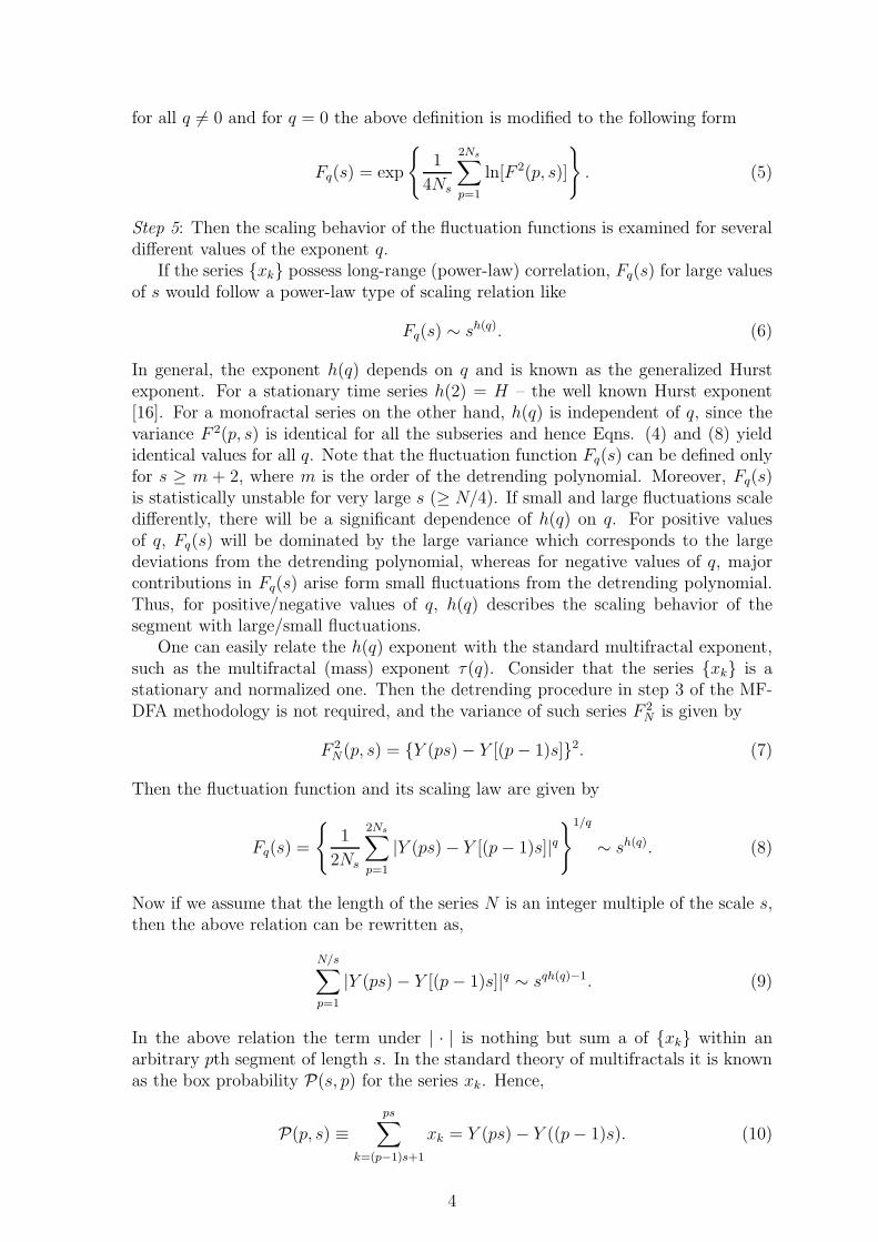
Figure 1: (a) Time series of the gold consumer price index and the correspondingreturn for the time period 1993–July 2013, (b) same as (a) but for the time period2010–July 2013.
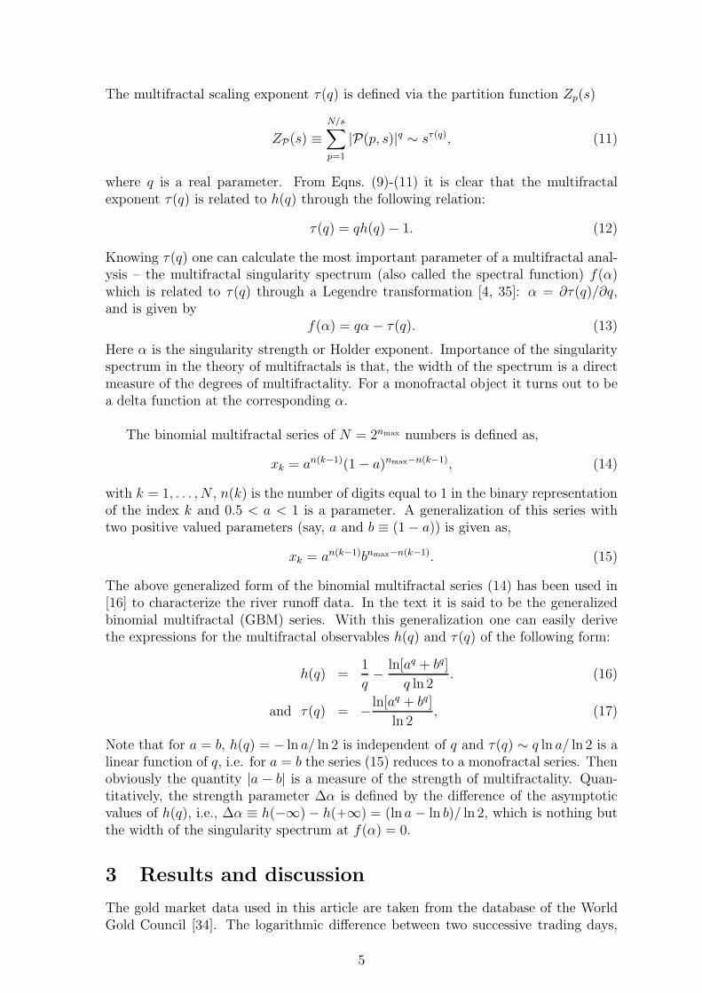
also known as return: R(T ) = lnP (T + 1)− lnP (T ), is used as the original series forthis analysis. To illustrate the nature of the series we show in Fig. 1(a) the CPI timeseries (upper panel) along with its returns (lower panel). The last section of theseseries shown in blue color are for the period of 2010–July 2013 and is magnified inFig. 1(b). In the text the first section, i.e. from 1993 to 2010, of the series is identifiedas series of period-I and the last section (from 2010 to July 2013) is identified as period-II. Note that, the time periods are explicitly mentioned in the diagrams. Figure 1demonstrates how the global gold market evolves with time. In Fig. 2 we show thelog-log plots of the cumulative distribution function (CDF) of normalized returns ofgold price indices for (a) the CPI and (b) the market series in China. The CDFsfor the other series analyzed here are more or less similar to 2(b) and hence are notshown here. However, the tail exponent, (ζ), gives the critical order of divergence ofmoments, is extracted from power-law regression for all the series. The ζ values areall found to vary from 3.04 to 3.5 for the long series, whereas for the series of period-II(2010-2013) the values are as high as 5.0 (for the CPI series).
The first indication for a power-law type of CDF of market return fluctuations canbe traced back to [36] and explicitly in stock markets [38, 37] the power-law is found
6
10-1 100 10110-3
10-2
10-1
100
10-1 100 101
Cum
ulat
ive
dist
ribu
tion
func
tion
Normalized return
Period 1993 - 2013 1993 - 2010 2010 - 2013
(a) Consumer price index (b) China
Period 1993 - 2013 1993 - 2010 2010 - 2013
Normalized return
Figure 2: Cumulative distribution function of the normalized returns of gold priceindices for three different time periods: (a) global consumer price index and (b) timeseries of China.
to be inverse cubic. Gabaix et al. [39] have given a theoretical interpretation of theabove empirical observations. In the case of gold market returns for the period 1968– 2010 the tail exponent is estimated to be ≈ 3, i.e. the CDF follows inverse cubicpower-law [40]. The effect of faster departure from the inverse cubic power-law in themore recent financial data, similar to the one shown in the present manuscript for thegold price time series in the period 2010–2013, is also shown in [41, 42, 43]. Recently,Rak et al. [44] indicate a possible more general applicability of the concept of Gabaixet al. [39] to the situations when the price fluctuations depart from the inverse cubicpower-law.
Long term correlated records {xi : i = 1, 2, . . .N} with zero mean and unit vari-ance are characterized by an autocorrelation function Cx(s) = 〈xixi+s〉 ≡ 1/(N −s)
∑N−si=1 xixi+s. If {xi} are uncorrelated, C(s) is zero for s > 0. Short-range correla-
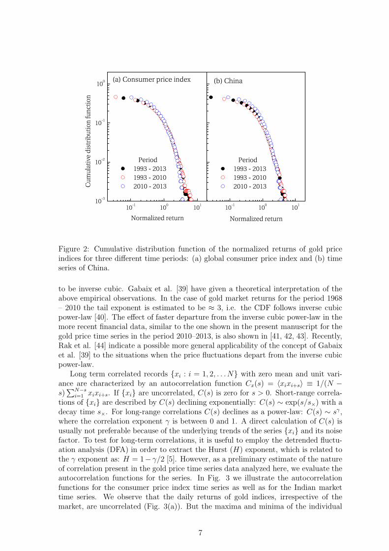
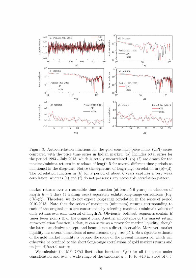
tions of {xi} are described by C(s) declining exponentially: C(s) ∼ exp(s/s×) with adecay time s×. For long-range correlations C(s) declines as a power-law: C(s) ∼ sγ ,where the correlation exponent γ is between 0 and 1. A direct calculation of C(s) isusually not preferable because of the underlying trends of the series {xi} and its noisefactor. To test for long-term correlations, it is useful to employ the detrended fluctu-ation analysis (DFA) in order to extract the Hurst (H) exponent, which is related tothe γ exponent as: H = 1−γ/2 [5]. However, as a preliminary estimate of the natureof correlation present in the gold price time series data analyzed here, we evaluate theautocorrelation functions for the series. In Fig. 3 we illustrate the autocorrelationfunctions for the consumer price index time series as well as for the Indian markettime series. We observe that the daily returns of gold indices, irrespective of themarket, are uncorrelated (Fig. 3(a)). But the maxima and minima of the individual
7
100 101 10210-3
10-2
10-1
100
100 101 10210-3
10-2
10-1
100
5 10 15 20 25 30 35-0.2
0.0
0.2
0.4
5 10 15 20 25 30 35-0.2
0.0
0.2
0.4
0.6
100 101 10210-3
10-2
10-1
100
0 200 400 600 800 1000
-0.06
-0.03
0.00
0.03
0.06
(d) Minima
Period: 1993-2013 CPI India
Lag
Aut
ocor
rela
tion
Aut
ocor
rela
tion
Aut
ocor
rela
tion
Lag
Period: 1993-2013 CPI India
(c) Maxima
(f) Minima Period: 2010-2013 CPI India
Lag
Period: 2010-2013 CPI India
(e) Maxima
Aut
ocor
rela
tion
Lag
(b) Maxima
Period: 2007-2013 CPI India
Lag
Aut
ocor
rela
tion
Aut
ocor
rela
tion
lag
CPI India
(a) Period: 1993-2013
Figure 3: Autocorrelation functions for the gold consumer price index (CPI) seriescompared with the price time series in Indian market. (a) Includes total series forthe period 1993 - July 2013, which is totally uncorrelated. (b)–(f) are drawn for themaxima/minima returns in windows of length 5 for several different time periods asmentioned in the diagrams. Notice the signature of long-range correlation in (b)–(d).The correlation function in (b) for a period of about 6 years captures a very weakcorrelation, whereas (e) and (f) do not possesses any noticeable correlation pattern.
market returns over a reasonable time duration (at least 5-6 years) in windows oflength R = 5 days (1 trading week) separately exhibit long-range correlations (Fig.3(b)-(f)). Therefore, we do not expect long-range correlation in the series of period2010-2013. Note that the series of maximum (minimum) returns corresponding toeach of the original ones are constructed by selecting maximal (minimal) values ofdaily returns over each interval of length R. Obviously, both sub-sequences contain Rtimes fewer points than the original ones. Another importance of the market returnautocorrelation function is that, it can serve as a proxy for market liquidity, thoughthe later is an elusive concept, and hence is not a direct observable. Moreover, marketliquidity has several dimensions of measurement (e.g., see [45]). So a rigorous estimateof the gold market liquidity is beyond the scope of the present manuscript, which willotherwise be confined to the short/long-range correlations of gold market returns andits (multi)fractal nature.
We calculate the MF-DFA2 fluctuation functions Fq(s) for all the series underconsideration and over a wide range of the exponent q : -10 to +10 in steps of 0.5.
8
The scaling behaviors of some of the fluctuation functions calculated from the CPIseries are illustrated in Fig. 4. Separate diagrams are drawn for the total series,period-I and period-II. Here the time scale s is varied from 6 to N/5, where N is theseries length. In the same figure we also show the Fq(s) functions generated from therandomly shuffled series (middle panel) as well as from the surrogated series (lowerpanel) corresponding to the original ones. The fluctuation functions calculated forthe other series under consideration also follow almost identical scale dependence asshown in the figure, and hence those diagrams are not included here. It is noticed thatthe multifractal results reasonably vary between the first and second order detrending,but the change is almost insignificant between the second and third or higher orderdetrending. Hence, the quadratic (second order) detrending is considered for thisanalysis. It is clear from Fig. 1 that the scaling behavior of Fq(s) for all three timeintervals as well as their shuffled and surrogated counterparts nicely follow the scaling-law (6) for s ≥ 10.
It is a known fact that there are two different types of multifractality may existin a time series data, namely (i) multifractality due to long-range time correlations ofthe small and large fluctuations and (ii) multifractality due to a fat-tailed probabilitydistribution function of the values in the series. The first kind of multifractality can beremoved by random shuffling of the given series and the corresponding shuffled serieswill exhibit monofractal scaling. Obviously, the probability distribution will not alterby random shuffling and hence the multifractality of the second kind will remainintact. If a given series contains both kinds of multifractality, the correspondingshuffled series will exhibit weaker multifractality than the original one. On the otherhand, the surrogate (phase randomization) analysis is an empirical technique of testingnonlinearity for a time series. The aim is to test whether the dynamics are consistentwith linearly filtered noise or a nonlinear dynamical system [46, 47]. The basic idea ofthe surrogate data method is to first specify some kind of linear stochastic process thatmimics “linear properties” of the original data. If the predictions (statistics) of theoriginal data are significantly different from those of surrogate series, we may considerthe presence of some higher order temporal correlations, i.e., the presence of dynamicnonlinearities. In this analysis we use the the null hypothesis, amplitude-adjustedFourier transform (AAFT) algorithm [48] to generate the surrogate series.
The generalized Hurst exponent h(q) is extracted from straight line fit to the log-logdata of Fq(s) versus s. We fit straight line in the 50 ≤ s ≤ 800 region for the total andthe period-I series, whereas the range chosen for the period-II series is 10 ≤ s ≤ 60.Note that, the fluctuation functions are found to obey the scaling law (6) better inthe mentioned scale regions. The order (q) dependence of the h(q) exponents is shownin Fig. 5 for the CPI series as well as for the price time series in China, India andTurkey. The lines in the diagrams represent the best fits of the GBM model (wheneverpossible) to the data points. The best fit parameter values are given in Table 1.The missing values in the table (and line in the figure) denote that the GBM modelcannot describe the corresponding time series. The figure shows that, irrespective ofthe series time duration, all the h(q) spectra representing the original series are orderdependent, though the dependency is weaker for the series of period-II. Moreover, thespectra obtained from the original series are more or less fitted to the GBM model,yielding Eqn. (16). hOWEVER, in some cases there is noticeable deviation betweenthe empirical values and the model around q ∼ 0 regions. The shuffled series, onthe other hand, produces h(q) spectra that are quite different from their originalcounterparts. In all cases but the CPI series of period-II, the total and period-I series
9
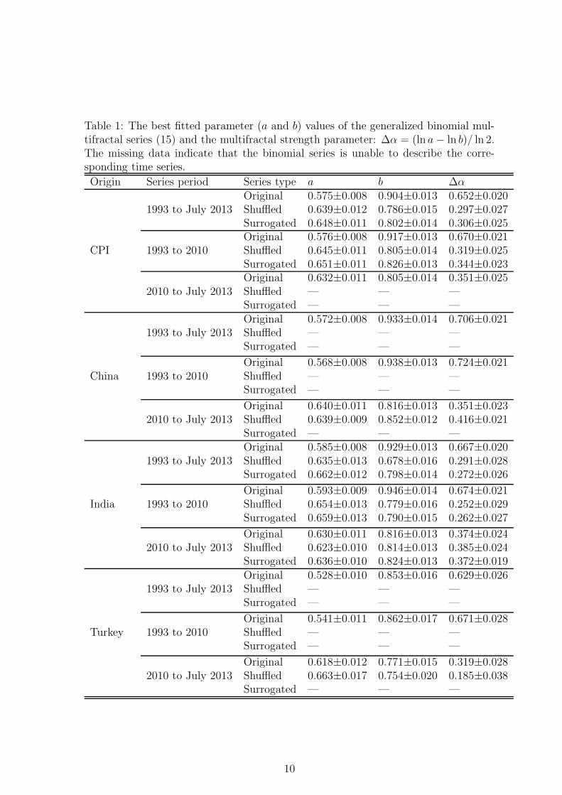
Table 1: The best fitted parameter (a and b) values of the generalized binomial mul-tifractal series (15) and the multifractal strength parameter: ∆α = (ln a− ln b)/ ln 2.The missing data indicate that the binomial series is unable to describe the corre-sponding time series.
Origin Series period Series type a b ∆αOriginal 0.575±0.008 0.904±0.013 0.652±0.020
1993 to July 2013 Shuffled 0.639±0.012 0.786±0.015 0.297±0.027Surrogated 0.648±0.011 0.802±0.014 0.306±0.025Original 0.576±0.008 0.917±0.013 0.670±0.021
CPI 1993 to 2010 Shuffled 0.645±0.011 0.805±0.014 0.319±0.025Surrogated 0.651±0.011 0.826±0.013 0.344±0.023Original 0.632±0.011 0.805±0.014 0.351±0.025
2010 to July 2013 Shuffled — — —Surrogated — — —Original 0.572±0.008 0.933±0.014 0.706±0.021
1993 to July 2013 Shuffled — — —Surrogated — — —
Original 0.568±0.008 0.938±0.013 0.724±0.021China 1993 to 2010 Shuffled — — —
Surrogated — — —
Original 0.640±0.011 0.816±0.013 0.351±0.0232010 to July 2013 Shuffled 0.639±0.009 0.852±0.012 0.416±0.021
Surrogated — — —Original 0.585±0.008 0.929±0.013 0.667±0.020
1993 to July 2013 Shuffled 0.635±0.013 0.678±0.016 0.291±0.028Surrogated 0.662±0.012 0.798±0.014 0.272±0.026
Original 0.593±0.009 0.946±0.014 0.674±0.021India 1993 to 2010 Shuffled 0.654±0.013 0.779±0.016 0.252±0.029
Surrogated 0.659±0.013 0.790±0.015 0.262±0.027
Original 0.630±0.011 0.816±0.013 0.374±0.0242010 to July 2013 Shuffled 0.623±0.010 0.814±0.013 0.385±0.024
Surrogated 0.636±0.010 0.824±0.013 0.372±0.019Original 0.528±0.010 0.853±0.016 0.629±0.026
1993 to July 2013 Shuffled — — —Surrogated — — —
Original 0.541±0.011 0.862±0.017 0.671±0.028Turkey 1993 to 2010 Shuffled — — —
Surrogated — — —
Original 0.618±0.012 0.771±0.015 0.319±0.0282010 to July 2013 Shuffled 0.663±0.017 0.754±0.020 0.185±0.038
Surrogated — — —
10
of China and Turkey, we observe a very weak order dependence of h(q) and the spectraare well described by the GBM model. In view of our previous discussion, the origin ofmultifractality in those series are both long-range temporal correlation and fat-tailedprobability distribution of the variables. In the exceptional cases, the shuffled seriesproduces h(q) spectra that are apparently consistent with an uncorrelated multifractalseries with power-law distribution function: P (x) = αx−(α+1) for 1 ≤ x < ∞ andα > 0. For the above series the generalized Hurst exponent is given as [7]: h(q) ∼ 1/qfor q > α and ∼ 1/α for q ≤ α, whereas τ(q) = q/α − 1 for q ≤ α and τ(q) = 0for q > α. Note that the multifractality of the above kind is originated purely froma fat-tailed probability distribution function. According to refs. [49, 50], the CPIseries for period-II, and the total and period-I series of China and Turkey, may beidentified as bifractals instead of multifractals. Our results on h(q) spectra apparentlycontradict the results of ref. [40], where it was possible to remove the multifractalityof the original series by random shuffling. In a similar analysis by Ghosh et al. [51]a q-dependent h(q) spectrum is observed for the shuffled series of gold indices. Butone should keep in mind that the series time period in those analysis are different,and the recent rapid changing values of gold indices may moderately change theresults. In our analysis the surrogate data generated by the AAFT procedure alsoresult in h(q) spectra that show significant amount of multifractality. The conjectureswill be more transparent when we will discuss the singularity spectrum. It is tobe noted that, in order to minimize the statistical error in the multifractal variablescorresponding to the shuffled/surrogated series, we take an average of h(q) values over10 shuffled/surrogated series corresponding to each of the original series.
The multifractal τ(q) exponents are plotted against q in Fig. 6 for all the seriesunder consideration. The lines in this figure also represent the binomial series, yieldingEqn. (17), with the same sets of parameters that are used optimiz the h(q) versus qdata and the parameters are given in Table 1. As already mentioned, for a monofractalseries τ(q) is linear with q, and any kind of nontrivial dynamics present in the datais reflected in the form of a nonlinear variation of τ(q) with q. The signature ofmultifractality in all the original series is clearly visible from their nonlinear variationagainst of τ(q) order number q. In some cases the shuffled series as well as thesurrogated series also show multifractality as strong as the original ones. Note thatthe observable τ(q) is directly calculated from h(q), therefore we do not put anyadditional emphasis on it. However, we would like to mention that the GBM modelreproduces the empirical τ(q) spectra very well.
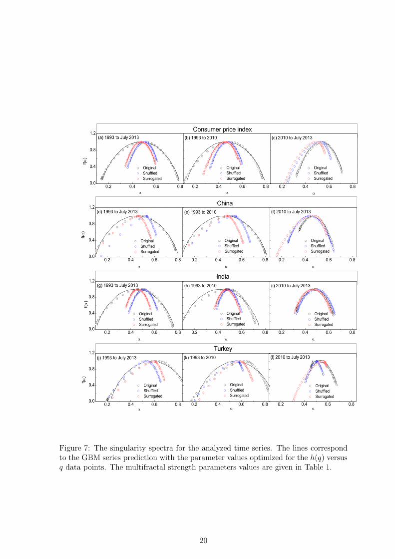
The most important results of a multifractal analysis is the singularity spectrum.To get a quantitative idea about the strength of multifractality, we calculate singu-larity spectra f(α) for the analyzed series and plot them in Fig. 7 against the Holderexponent α. From the top to the bottom panel the diagrams represent, respectivelythe CPI time series, the price time series in China, India and Turkey. The solid linesin this figure also indicate the GBM series with the parameter values as given Table1). As we know that the width of singularity spectrum is a measure of multifractality,the multifractal nature of all the original series is well reflected by the correspondingsingularity spectrum. All the shuffled series within the time period 1993-July 2013show much weaker multifractality than the corresponding original series. The same istrue for the period-I series as well. But for the period-II shuffled series the singularityspectral widths are almost as equal as to their original counterparts. The observa-tions here are consistent with our autocorrelation analysis that is, the time series forthe period 2010–July 2013 does not capture long-range correlation, and hence the ob-
11
served multifractal nature of these series arise purely from the probability distributionfunctions of their indices. The shuffled series generated spectra, as it is expected, areall centered around α ≈ 0.5. In some cases (especially Fig. 7(j) and (k)) the peakposition of the f(α) spectrum is obtained at a slightly higher value of α. A similarobservation is also made in [52], where it is shown that the peak position as well as thewidth of a multifractal spectrum may vary with its length along with its type. Thesurrogated series, irrespective of its time period, reproduce stable multifractal spectrabut much narrower than the corresponding empirical ones. The strength parameterof multifractality (∆α) is measured as the width of singularity spectrum at f(α) = 0.Analytically that corresponds to ∆α = (ln a− ln b)/ ln 2. Using the (a, b) parametervalues we calculate the ∆α values and are presented in the extreme right columnof Table 1. Here we will get a clear and quantitative difference among the variousseries studied. As can be seen in the table that the strength of multifractality for theoriginal long and period-I series is always about two times that of the period-II series,while the difference between ∆αs of the original and the shuffled/surrogated series(whenever possible to fit the GBM model) for the series of period-II is marginal. Theobservations indicate that, except the market series in China and India for period-II,the observed multifractality in the analyzed gold price indices are partly due to thelong-range time correlation and partly due to the fat-tailed distribution function ofthe values, and in the exceptional cases it is mainly due to the probability densityfunction of the indices; for which we expect ∆α(original) ≈ ∆α(shuffled). The sur-rogated data generated f(α) spectra in all cases but the series of Turkey are shiftedtowards the lower α side than their shuffled one, but they produce ∆α value almostidentical to that of the shuffled series. In case of the market of Turkey we find nochange in the day-to-day market return index in several places, and some times theindex remains constant over a wide section of the series. That might be a reason forthe exceptional behavior of the market of Turkey.
4 Conclusion
Multifractal nature of (i) the consumer price index time series of gold and (ii) the goldmarket time series of China, Indian and Turkey during the period 1993–July 2013,has been investigated in terms of the multifractal detrended fluctuation analysis. Forbetter understanding of the rapidly increasing and fluctuating market trend over thelast few years we divide each series into two: first section from 1993 to 2010 (period-I)and second section from 2010 to July 2013 (period-II). That is, all together 12 originalseries, corresponding to each of them a randomly shuffled and a surrogated series, areanalyzed. Multifractal observables, such as the generalized Hurst exponents (h(q)),multifractal exponent (τ(q)) and singularity spectrum (f(α)) for all the series, areextracted and are fitted (whenever possible) to the generalized binomial multifractalmodel series. The following conclusions can be drawn from the our analysis.
The MF-DFA fluctuation functions for all the analyzed time series nicely followthe scaling law (6), as is expected for a multifractal series. The generalized Hurstexponent spectra corresponding to the original series are found to be order dependentand are fitted more or less by the GBMmodel. The shuffled series as well as the AAFTsurrogated series also produce order dependent h(q) spectra, but the order dependenceis much weaker than the original series. The nature of the h(q) spectra are consistentwith the fact that the multifractality in the long-term CPI time series as well as inthe market trend of India is generated from both the long-range temporal correlation
12
and the probability distribution of the series values. In the case of the market series ofChina and Turkey the origin of multifractality is found to be the fat-tailed probabilitydistribution function, and hence the binomial series (15) cannot describe those series.The observed multifractality for period-II is mainly due to the probability densityfunction. The τ(q) exponent diagrams reflect identical features of the data as theh(q) diagrams do. The multifractal singularity spectra for all the original long seriesare significantly wider than the corresponding shuffled and/or surrogated spectra. Forperiod-II the original and shuffled series produce almost identical singularity spectrathat strengthen the observations of the h(q) spectra.
It is obvious that the market series and the CPI series are highly correlated.Therefore, a cross-correlation study [53] between the individual market series andmarket-CPI series may reveal more insight into the gold market pattern.
References
[1] B. B. Mandelbrot, The Fractal Geometry of Nature, Freeman, New York, 1982.
[2] H. E. Hurst, Transact. Am. Soc. Civil Eng., 116 (1951) 770-799.
[3] H. E. Hurst, R. P. Black and Y. M. Simaika, Long-Term Storage: An Experi-mental Study, Constable, London, 1965.
[4] J. Feder, Fractals, Plenum Press, New York, 1988.
[5] C. -K. Peng, S. V. Buldyrev, S. Havlin, M. Simons, H. E. Stanley and A. L.Goldberger, Mosaic organization of DNA nucleotides, Phys. Rev. E 49 (1994)1685-1689.
[6] E. Bacry, J. Delour and J. F. Muzy, Multifractal random walk, Phys. Rev. E 64(2001) 026103-026107.
[7] J. W. Kantelhardt, S. A. Zschiegner, E. Koscielny-Bunde, S. Havlin, A. Bundeand H. E. Stanley, Multifractal detrended uctuation analysis of nonstationarytime series, Physica A 316 (2002) 87-114.
[8] K. Matia, Y. Ashkenazy and H. E. Stanley, Multifractal properties of price fluc-tuations of stocks and commodities, Europhys. Lett. 61 (2003) 422-428.
[9] P. Oswiecimka, J. Kwapien and S. Drozdz, Multifractality in the stock market:price increments versus waiting times, Physica A 347 (2005) 626-638.
[10] P. Oswiecimka, J. Kwapien and S. Drozdz, Wavelet versus detrended fluctuationanalysis of multifractal structures, Phys. Rev. E 74 (2006) 016103-016120.
[11] J. Kwapien, P. Oswiecimka and S. Drozdz, Components of multifractality inhigh-frequency stock returns, Physica A 350 (2005) 466-474.
[12] Y. Wang, Y. Wei and C. Wu, Analysis of the efficiency and multifractality ofgold markets based on multifractal detrended fluctuation analysis, Physica A390 (2011) 817-827.
[13] S. Samadder, K. Ghosh and T. Basu, Fractal analysis of prime Indian stockmarket indices, Fractals 21 (2013) 1350003-1350017.
13
[14] X. Lu, J. Tian, Y. Zhou and Z. Li, Multifractal detrended fluctuation analysis ofthe Chinese stock index futures market, Physica A 392 (2013) 1452-1458.
[15] P. Mali, Fluctuation of gold price in India versus global consumer price index,Fractals 22(1) (2014) 1450004 (9pp).
[16] J. W. Kantelhardt, D. Rybski, S. A. Zschiegner, P. Braun, E. Koscielny-Bunde,V. Livina, S. Havlin and A. Bunde, Multifractality of river runo and precipitation:comparison of fluctuation analysis and wavelet methods, Physica A 330 (2003)240-245.
[17] E. Koscielny-Bunde, J. W. Kantelhardt, P. Braun, A. Bunde and S. Havlin, Long-term persistence and multifractality of river runoff records: Detrended fluctuationstudies, Journal of Hydrology 322 (2006) 120-137.
[18] K. Shi, W.-Y. Li, C.-Q. Liu and Z.-W. Huang, Multifractal fluctuations of ji-uzhaigou tourists before and after wenchuan earthquake, Fractals 21 (2013)1350001-1350008.
[19] R. Benicio, T. Stosic, P.H. de Figueiredo, B.D. Stosic, Multifractal behavior ofwild-land and forest fire time series in Brazil, Physica A 392 (2013) 6367-6374.
[20] T. B. Veronese, R. R. Rosa, M. J. A. Bolzan, F. C. R. Fernandes, H. S. Sawant andM. Karlicky, Fluctuation analysis of solar radio bursts associated with geoeffectiveX-class flares, Journal of Atmospheric and Solar-Terrestrial Physics 73 (2011)1311-1316.
[21] F. Liao, B. D. Struck, M. Macrobert and Y.-K. Jan, Multifractal analysis ofnonlinear complexity of sacral skin blood flow oscillations in older adults, Medical& Biological Engineering 49(8) (2001) 925-934.
[22] F. Esen, S. Caglar, N. Ata, T. Ulus, A. Birdane and H. Esen, Fractal scalingof laser Doppler flowmetry time series in patients with essential hypertension,Microvascular Research 82(3) (2011) 291-295.
[23] S. Kumar, L. Gu, N. Ghosh and S. K. Mohanty, Multifractal detrended fluctu-ation analysis of optogenetic modulation of neural activity, Proc. Optogenetics:Optical Methods for Cellular Control, 858608 (2013).
[24] N. Cardenas, S. Kumar and S. Mohanty, Dynamics of cellular response to hy-potonic stimulation revealed by quantitative phase microscopy and multi-fractaldetrended fluctuation analysis, Appl. Phys. Lett. 101 (2012) 203702-203706.
[25] Y. X. Zhang, W. Y. Qian and C. B. Yang, Multifractal structure of pseudorapidityand azimuthal distributions of the shower particles in Au+Au collisions at 200A GeV, Int. J. Mod. Phys. A 23 (2008) 2809-2816.
[26] X. Wang and C. B. Yang, Fractal properties of particles in phase space fromURQMD model, Int. J. Mod. Phys. E 22 (2013) 1350021-1350029.
[27] P. A. Varotsos, N. V. Sarlis and E. S. Skordas, arXiv:0904.2465 [cond-mat.stat-mech].
14
[28] M. Ignaccolo, M. Latka and B. J. West, Detrended fluctuation analysis of scalingcrossover effects, Europhys. Lett. 90 (2010) 10009-10015.
[29] M. P. M. A. Baroni, A. De Wit and R. R. Rosa, Detrended fluctuation analysisof numerical density and viscous fingering patterns, Europhys. Lett. 92 (2010)64002-64008.
[30] J. S. Murguia, M. M. Carlo, M. T. Ramirez-Torres and H. C. Rosu, Waveletmultifractal detrended fluctuation analysis of encryption and decryption matrices,Int. J. Mod. Phys. C 24 (2013) 1350069-82.
[31] R. N. Mantegna and H. E. Stanley, An introduction to Econophysics, CambridgeUniversity Press, Cambridge, 1999.
[32] J. P. Bouchaud and M. Potters, Theory of Financial Risk, Cambridge UniversityPress, Cambridge, 2000.
[33] J. Kwapien and S. Drozdz, Physics approach to complex systems, Phys. Rep. 515(2012) 115-226.
[34] World Gold Council, www.gold.org.
[35] H. -O. Peitgen, H. Jurgens and D. Saupe, Chaos and Fractals, Appendix B,Springer, New York, 1992.
[36] T. Lux, The stable paretian hypothesis and the frequency of large returns: Anexamination of major german stocks, Appl. Finan. Econ. 6 (1996) 463475.
[37] P. Gopikrishnan, V. Plerou, L. A. N. Amaral, M. Meyer and H. E. Stanley,Scaling of the distribution of fluctuations of financial market indices, Phys. Rev.E 60 (1999) 5305-5316.
[38] P. Gopikrishnan, M. Meyer, L. A. N. Amaral, and H. E. Stanley, Inverse cubic lawfor the distribution of stock price variations, Eur. Phys. J. B 3 (1998) 139-140.
[39] X. Gabaix, P. Gopikrishnan, V. Plerou and H. E. Stanley, Institutional investorsand stock market volatility, Quart. J. Econ. 121 (2006) 461-504.
[40] M. Bolgorian and Z. Gharli, A multifractal detrended fluctuation analysis of goldprice fluctuations, Acta Phys. Pol. B 42 (2011) 159-169.
[41] S. Drozdz, J. Kwapien, F. Gruemmer, F. Ruf and J. Speth, Are the contemporaryfinancial fluctuations sooner converging to normal?, Acta Phys. Pol. B 34 (2003)4293-4306.
[42] S. Drozdz, M. Forczek, J. Kwapien, P. Oswiecimka and R. Rak, Stock marketreturn distributions: from past to present, Physica A 383 (2007) 59-64.
[43] S. Drozdz, J. Kwapien, P. Oswiecimka and R. Rak, The foreign exchange mar-ket: return distributions, multifractality, anomalous multifractality and the Eppseffect, New Journal of Physics 12 (2010) 105003 (23pp).
[44] R. Rak, S. Drozdz, J. Kwapiee, P. Oswicimka, Stock returns versus trading vol-ume: is the correspondence more general?, Acta Phys. Pol. B, 44 (2013) 2035-2050.
15
[45] Y. Amihud, H. Mendelson and H. Pedersen, Liquidity and asset prices, Founda-tions and Trends in Finance 1 (2005) 269-364.
[46] G. E. Uhlenbeck and L. S. Ornstein, On the Theory of the Brownian Motion,Phys. Rev. 36 (1930) 823-841.
[47] C. Rath, M. Gliozzi, I. E. Papadakis and W. Brinkmann, Revisiting algorithmsfor generating surrogate time series, Phys. Rev. Lett. 109 (2012) 144101-144106.
[48] J. Theiler, S. Eubank, A. Longtin, B. Galdrikian and J. D. Farmer, Testing fornonlinearity in time series: the method of surrogate data, Physica D 58 (1992)77-94.
[49] H. Nakao, Multi-scaling properties of truncated Levy flights, Phys. Lett. A 266(2000) 282-289.
[50] S. Drozdz, J. Kwapien, P. Oswiecimka and R. Rak, Quantitative features ofmultifractal subtleties in time series, Europhys. Lett. 88 (2009) 60003.
[51] D. Ghosh, S. Dutta and S. Samanta, Fluctuation of gold price: a multifractalapproach, Acta Phys. Plo. B 43 (2012) 1261-1274.
[52] D. Grech and L. Czarnecki, Multifractal dynamics of stock markets, Acta Phys.Pol. A 117 (2010) 623-629.
[53] D. Horvatic, H. E. Stanley and B. Podobnik, Detrended cross-correlation analysisfor non-stationary time series with periodic trends, Europhys. Lett. 94 (2011)18007.
16
101 102 10310-4
10-3
10-2
10-1
101 102 103 101 102
101 102 10310-4
10-3
10-2
10-1
101 102 103 101 102
101 102 10310-4
10-3
10-2
10-1
101 102 103 101 102
F q(s)
s
q = -10 q = -5 q = -3 q = -1 q = 0 q = 1 q = 3 q = 5 q = 10
(a) 1993 to July 2013
Surrogated CPI series
Shuffled CPI series
(b) 1993 to 2010
s
Original CPI series (c) 2010 to July 2013
s
q = -10 q = -5 q = -3 q = -1 q = 0 q = 1 q = 3 q = 5 q = 10
(d) 1993 to July 2013
F q(s)
s
(e) 1993 to 2010
s
(f) 2010 to July 2013
s
(g) 1993 to July 2013
q = -10 q = -5 q = -3 q = -1 q = 0 q = 1 q = 3 q = 5 q = 10
F q(s)
s
(h) 1993 to 2010
s
(i) 2010 to July 2013
s
Figure 4: The MF-DFA2 fluctuation functions Fq(s) for the consumer price indexseries of gold plotted with scale s for three different time duration: (a) 1993–July2013, (b) 1993–2010 and (c) 2010–July 2013. Predictions from the shuffled series(middle panel) and the surrogated series (bottom panel) corresponding to the originalones are also shown.
17
-10 -5 0 5 10 -10 -5 0 5 10-10 -5 0 5 10
0.2
0.4
0.6
0.8
-10 -5 0 5 10
0.2
0.4
0.6
0.8
-10 -5 0 5 10 -10 -5 0 5 10
-10 -5 0 5 10
0.2
0.4
0.6
0.8
-10 -5 0 5 10 -10 -5 0 5 10
-10 -5 0 5 10
0.2
0.4
0.6
0.8
-10 -5 0 5 10 -10 -5 0 5 10
Original
Shuffled
Surrogated
q
(b) 1993 to 2010
Original
Shuffled
Surrogated
(c) 2010 to July 2013
q
Turkey
India
China
(a) 1993 to July 2013
h(q)
q
Original
Shuffled
Surrogated
Consumer price index
(d) 1993 to July 2013
Original
Shuffled
Surrogated
h(q)
Original
Shuffled
Surrogated
(e) 1993 to 2010
q
Original
Shuffled
Surrogated
(f) 2010 to July 2013
q
Original
Shuffled
Surrogated
(g) 1993 to July 2013
q
q
h(q)
q
Original
Shuffled
Surrogated
(h) 1993 to 2010
Original
Shuffled
Surrogated
(i) 2010 to July 2013
q
Original
Shuffled
Surrogated
(j) 1993 to July 2013
h(q)
q
Original
Shuffled
Surrogated
(k) 1993 to 2010
q
Original
Shuffled
Surrogated
(l) 2010 to July 2013
q
Figure 5: The generalized Hurst exponent h(q) spectra for the analyzed time series.The lines correspond to the GBM series (15), yielding Eqn. (16). The best fit param-eter values are quoted in Table 1.
18
-10 -5 0 5 10 -10 -5 0 5 10-10 -5 0 5 10-10
-5
0
5
-10 -5 0 5 10-10
-5
0
5
-10 -5 0 5 10 -10 -5 0 5 10
-10 -5 0 5 10-10
-5
0
5
-10 -5 0 5 10 -10 -5 0 5 10
-10 -5 0 5 10-10
-5
0
5
-10 -5 0 5 10 -10 -5 0 5 10
Original
Shuffled
Surrogated
q
(b) 1993 to 2010
Original
Shuffled
Surrogated
(c) 2010 to July 2013
q
Turkey
India
China
(a) 1993 to July 2013
(q)
q
Original
Shuffled
Surrogated
Consumer price index
(d) 1993 to July 2013
Original
Shuffled
Surrogated
(q)
Original
Shuffled
Surrogated
(e) 1993 to 2010
q
Original
Shuffled
Surrogated
(f) 2010 to July 2013
q
Original
Shuffled
Surrogated
(g) 1993 to July 2013
q
q
(q)
q
Original
Shuffled
Surrogated
(h) 1993 to 2010
Original
Shuffled
Surrogated
(i) 2010 to July 2013
q
Original
Shuffled
Surrogated
(j) 1993 to July 2013
(q)
q
Original
Shuffled
Surrogated
(k) 1993 to 2010
q
Original
Shuffled
Surrogated
(l) 2010 to July 2013
q
Figure 6: The multifractal τ(q) exponent spectra for the analysed time series. Thelines correspond to the GBM series (15), yielding Eqn. (17) with the same set ofparameters as optimized for the h(q) versus q data points (see Table 1).
19
0.2 0.4 0.6 0.80.2 0.4 0.6 0.80.2 0.4 0.6 0.80.0
0.4
0.8
1.2
0.2 0.4 0.6 0.80.0
0.4
0.8
1.2
0.2 0.4 0.6 0.8 0.2 0.4 0.6 0.8
0.2 0.4 0.6 0.80.0
0.4
0.8
1.2
0.2 0.4 0.6 0.8 0.2 0.4 0.6 0.8
0.2 0.4 0.6 0.80.0
0.4
0.8
1.2
0.2 0.4 0.6 0.8 0.2 0.4 0.6 0.8
Turkey
India
China
(c) 2010 to July 2013
Original Shuffled Surrogated
Consumer price index(b) 1993 to 2010
Original Shuffled Surrogated
f()
Original Shuffled Surrogated
(a) 1993 to July 2013
Original Shuffled Surrogated
(d) 1993 to July 2013
f()
Original Shuffled Surrogated
(e) 1993 to 2010
Original Shuffled Surrogated
(f) 2010 to July 2013
Original Shuffled Surrogated
(g) 1993 to July 2013
f()
Original Shuffled Surrogated
(h) 1993 to 2010
Original Shuffled Surrogated
(i) 2010 to July 2013
Original Shuffled Surrogated
(j) 1993 to July 2013
f()
Original Shuffled Surrogated
(k) 1993 to 2010
Original Shuffled Surrogated
(l) 2010 to July 2013
Figure 7: The singularity spectra for the analyzed time series. The lines correspondto the GBM series prediction with the parameter values optimized for the h(q) versusq data points. The multifractal strength parameters values are given in Table 1.
20