Embed Size (px)
Citation preview
MPRAMunich Personal RePEc Archive
Assessing Municipal Bond DefaultProbabilities
Matthew Holian and Marc Joffe
San Jose State University, Public Sector Credit Solutions
30. April 2013
Online at http://mpra.ub.uni-muenchen.de/46728/MPRA Paper No. 46728, posted 5. May 2013 20:31 UTC
Assessing Municipal Bond Default Probabilities
Matthew J. Holian, Ph.D.
Associate Professor of Economics
San Jose State University
1 Washington Square Hall
San Jose, CA 95192-0114
Tel: (408) 457-4367
E-mail: [email protected]
Marc D. Joffe
Principal Consultant
Public Sector Credit Solutions
1955 N. California Blvd.
Walnut Creek, CA 94596
Tel: (415) 578-0558
Email: [email protected]
DRAFT submitted to the California Debt and Investment Advisory
Commission and the Center for California Studies and for peer
review. This document reflects the opinions of the authors and not
necessarily those of CDIAC or the Center.
DRAFT ii DRAFT
Abstract
In response to a request from the California Debt and Investment Advisory Commission, we
propose a model to estimate default probabilities for bonds issued by cities. The model can be used
with financial data available in Comprehensive Annual Financial Reports that cities are required to
publish. The study includes modeled default probability estimates for 261 California cities with
population over 25,000. Our model relies on case study evidence, logistic regression analysis of
major city financial statistics from the Great Depression – the last time a large number of cities
defaulted – as well as logistic regression analysis of more recent city financial statistics.
Independent variables in our model include (1) the ratio of interest and pension expenses to total
revenue, (2) the annual change in total revenue, (3) the ratio of general fund surplus (or deficit) to
general fund revenues and (4) the ratio of general fund balance to general fund expenditures.
DRAFT iii DRAFT
Table of Contents:
Executive Summary.............................................................................................................................................. v
Acknowledgements ............................................................................................................................................ vii
Introduction ....................................................................................................................................................... - 1 -
Literature Review ............................................................................................................................................ - 6 -
Previous Depression-Era Municipal Default Research ................................................................. - 6 -
Predicting Credit Ratings as a Proxy for Estimating Default Risk ............................................ - 9 -
Objections to Rating Based Analysis ................................................................................................. - 13 -
Estimating Default Probability from Market Prices .................................................................... - 16 -
Default Probability Modeling Using Logit and Probit Techniques ........................................ - 18 -
Great Depression Review and Analysis ................................................................................................ - 22 -
The Depression Era Municipal Default Wave ................................................................................ - 23 -
Bank Closings, Bank Holidays and Municipal Bond Defaults .................................................. - 24 -
Property Tax Delinquencies ................................................................................................................. - 25 -
Public Employee Pensions .................................................................................................................... - 27 -
Data Selection ............................................................................................................................................ - 29 -
Conceptual Model and Variable Selection ...................................................................................... - 31 -
Statistical Methodology ......................................................................................................................... - 37 -
Limitations .................................................................................................................................................. - 41 -
Municipal Bond Defaults in California: History and Case Studies .............................................. - 42 -
Pre-1930 ...................................................................................................................................................... - 42 -
Depression Era .......................................................................................................................................... - 45 -
Post 1940 ..................................................................................................................................................... - 47 -
Desert Hot Springs ................................................................................................................................... - 49 -
Vallejo ........................................................................................................................................................... - 53 -
DRAFT iv DRAFT
Mammoth Lakes ....................................................................................................................................... - 59 -
Stockton ....................................................................................................................................................... - 60 -
San Bernardino ......................................................................................................................................... - 65 -
Special District Bond Defaults ............................................................................................................. - 68 -
Redevelopment Agency Defaults ....................................................................................................... - 69 -
City Fiscal Emergencies ......................................................................................................................... - 70 -
Concluding Comments............................................................................................................................ - 72 -
City Bond Defaults and Bankruptcies outside California .............................................................. - 73 -
The 1970’s ................................................................................................................................................... - 73 -
More Recent Experience in Other States ......................................................................................... - 76 -
Recent Data Analysis and a Hybrid Model .......................................................................................... - 92 -
Addressing Public Employee Pensions and OPEBs ..................................................................... - 92 -
Statistical Analysis of Contemporary Data ..................................................................................... - 94 -
Creating a Hybrid Model ........................................................................................................................ - 99 -
Limitations and Future Research .................................................................................................... - 103 -
Conclusion..................................................................................................................................................... - 105 -
Appendix 1: Extending the Depression-Era Default Model ....................................................... - 107 -
Appendix 2: Comparing data: CAFRs and the SCO’s Cities Annual Report .......................... - 122 -
Appendix 3: Default Probability Scores for California Cities .................................................... - 126 -
References .................................................................................................................................................... - 134 -

DRAFT v DRAFT
DRAFT vi DRAFT
Executive Summary
California local agencies have faced substantial fiscal stress in the aftermath of the
financial crisis. Several cities have filed for bankruptcy, defaulted on bond payments or
declared fiscal emergencies. However, the vast majority of California local bond issuers
continue to perform on their obligations.
The fiscal troubles faced by individual governments typically receive substantial
publicity. Such news reports reinforce dire predictions from high profile analysts that a
municipal market crisis is imminent. As a result, bondholders may be dissuaded from
investing in the obligations of all municipal bond issuers – even those that are relatively
healthy. This phenomenon threatens to exacerbate municipal bond market illiquidity,
which, according to Ang & Green (2011), already costs issuers an extra 1.1% in annual
interest.
With the collapse of the municipal bond insurance business and questions
concerning the credibility of bond ratings, new methods of credit risk assessment are
required. In response to a request by the California Debt and Investment Advisory
Commission, we have created an empirically-based methodology for assigning credit
scores to municipalities, using quantitative techniques that are resistant to bias. These
scores take the form of default probabilities and are based on a modeling procedure often
applied to corporate borrowers. Using this methodology, we have assigned default
probability scores to over 260 California cities with population over 25,000 that have filed
2011 or 2012 Comprehensive Annual Financial Reports.
In bond market terms, a default is usually defined as the failure on the part of an
issuer to pay principal and/or interest in full and on a timely basis. It is this definition of
DRAFT vii DRAFT
default that we use in this study. This means we do not consider the concept of a technical
default which often relates to the failure of an issuer to carry out other obligations under
the bond agreement, such as the prompt filing of continuing disclosures. Further, we do not
consider failure to pay contractors, employees, retirees or beneficiaries promised sums as
defaults for the current purpose – the concept narrowly applies to bondholders.
Since our model applies to cities themselves, it does not consider the specific
attributes of their individual bond issues. Thus, general obligation bonds issued by a city
should be expected to have less risk than our estimates suggest, while certificates of
participation and other securities not explicitly backed by a diverse stream of tax revenues
may be more risky.
Our model of municipal default risk is based on four fiscal indicators. These are: (1)
the ratio of interest and pension expenses to total governmental fund revenue, (2) the
annual change in total governmental fund revenue, (3) the ratio of the city’s general fund
surplus or deficit to its general fund revenue and (4) the ratio of the city’s end of year
general fund balance to its general fund expenditures. In the study, we provide statistical
and case study evidence to support the choice of these variables and appropriate
coefficients.
We hope that the proposed model will help municipal bond investors and other
stakeholders in city government solvency better comprehend the risks faced by municipal
issuers. We also hope that other researchers and practitioners will become interested in
this topic and our analytical approach, so that they will build upon and improve our
findings.
DRAFT viii DRAFT
Acknowledgements
The authors wish to thank members of the research team that assembled the
research data and created the technology needed to analyze and present both the data and
analysis. These contributors, in alphabetical order, include Tracy Berhel, Charlie Deist,
Peter Dzurjanin, Michal Kevicky, Karthick Palaniappan, T. Wayne Pugh, Ivar Shanki and
Charles Tian. Valuable information appearing in this study was also contributed by Carrie
Drummond, Dr. Robert Freeman and Triet Nguyen. Data about California municipal bonds
was generously contributed by Mergent Corporation. We also wish to thank the many city
financial officials who responded to data requests so promptly and completely. This project
convinces us that most municipal finance officers are dedicated to accurately reporting the
financial results for their communities and to freely sharing their calculations with the
public. Finally, we wish to thank the California Debt and Investment Advisory Commission
and the Center for California Studies for giving us the opportunity to conduct this research.
These acknowledgments notwithstanding, the responsibility for errors and omissions
remain with us.
Matthew Holian and Marc Joffe
April 30, 201
DRAFT 1 DRAFT
Introduction
The issue of municipal solvency has frequently made the headlines in recent years.
Meredith Whitney’s 2010 appearance on 60 Minutes was but one of a number of dire
predictions for municipal bondholders. In 2012, the bankruptcies of Stockton and San
Bernardino attracted significant media attention, as has the state takeover of Detroit,
Michigan earlier this year.
Unfortunately for bondholders and the many other stakeholders in city solvency, the
debate about municipal credit has been often generated more heat than light. Whitney’s
analysis fed into a narrative about skyrocketing public employee pension costs triggering a
tsunami of municipal bankruptcies.
These politically charged predictions have yet to be borne out by the facts on the
ground. In the 60 Minutes interview, Whitney predicted 50-100 sizable defaults (CBS News,
2010). She later stated that this would be a “something to worry about” within 12 months
of her appearance which occurred in December 2010. When it became apparent that this
dire forecast was failing to materialize, Michael Lewis (2011) wrote an influential piece in
Vanity Fair quoting Whitney as saying “who cares about the stinking muni-bond market?”
and attempting to rehabilitate her by turning the reader’s attention to fiscal problems in
California cities, public employee pensions and the risk of “cultural” as opposed to financial
bankruptcy.
For those who do care about the “stinking” municipal bond market, the discussion
left much to be desired. Investors are still wondering how much risk they actually shoulder
when purchasing municipal bonds issued by California cities and how much extra interest
they should expect to receive in compensation for taking on this risk. The question of the
DRAFT 2 DRAFT
appropriate interest rate resonates far beyond the municipal bond market, since it directly
affects municipal debt service costs, which in turn impact tax rates, service levels and cities’
ability to add infrastructure by borrowing.
As we discuss in this study, defaults by cities have been quite rare since the Great
Depression. Doty (2012) estimates that annual default rates on general obligation bonds
have been consistently below 0.1% in recent decades. Indeed, a researcher is compelled to
unearth 80-year old data just to obtain a statistically meaningful sample of general
obligation bond defaults on the part of US cities. Even when this dark period in the history
of municipal finance is investigated, we find the defaults were often the result of
idiosyncratic factors that don’t portend ill for modern investors. Finally, pension
underfunding is not a new phenomenon: as Munell (2012) documents, it was also a serious
concern in the 1970s – a period that witnessed some highly publicized city financial
emergencies, but no spate of municipal bond defaults.
All that said, defaults have occurred and will continue to occur, perhaps with
somewhat greater frequency than they have in recent decades. Clearly, some cities are
more at risk than others, and so stakeholders would benefit from objective, widely
available measures of municipal credit risk.
While credit rating agencies have the potential to better inform the public’s
understanding of municipal credit risk, they face several barriers in doing so. First, since
they rely primarily on bond issuers for their revenue, they have limited incentive to
evaluate cities they are not paid to rate. Second, much of their investor-oriented research is
sold as premium content and thus cannot be freely distributed. Third, rating agencies have
lost credibility in the aftermath of the 2008 financial crisis. And, finally, the three major
DRAFT 3 DRAFT
rating agencies were sued by the Connecticut attorney general – also in 2008 – for
assigning overly harsh ratings to municipal bond issuers relative to corporate and
structured finance issuers. Two of the three agencies recalibrated their municipal ratings in
response to the suit, which was settled in 2011 with no admission of responsibility but the
extension of credits to the state of Connecticut for future ratings services.
We believe that the informational vacuum created by the rating agency problem can
be filled by academic research. This study represents our initial contribution to this
academic project, and we hope that it will motivate others to add their insights. Our
approach involves the use of statistical and case study analysis to create a municipal bond
default probability model targeted at California cities with population greater than 25,000.
The discussion proceeds as follows. First, we provide a literature review which
discusses previous efforts to model municipal credit quality. We find that most of the
literature uses ratings or bond yields as a proxy for credit risk, and offer objections to these
approaches.
Next, we review the Depression-era municipal bond default experience and propose
a simple logit model based on a set of data collected from this period. This analysis
identifies two significant variables intuitively related to default risk: the ratio of interest to
revenue and the change in annual revenue.
After this, we provide a comprehensive review of California city bond defaults and
bankruptcies with case studies of the most recent payment difficulties. The case study
evidence suggests that exhaustion of the general fund – an element that is not available in
the Great Depression data set – has been a major driver in recent bankruptcy filings and
attendant defaults.
DRAFT 4 DRAFT
We then survey post-Depression defaults in US cities outside California. As part of
this discussion, we see how New York and Cleveland – both of which defaulted in the 1970s
– ranked against peer cities with respect to variables of interest. We also provide
information that supplies much needed context to popular media reporting about
municipal bond distress. Specifically, we find that bankruptcy does not necessarily involve
default (and vice versa) and that most bankruptcies have occurred in small towns, many of
which did not have significant volumes of outstanding municipal bonds (if any).
Finally, we propose a second model based on more recent data that enables us to
test the relative significance of general fund surplus/deficit and general fund balance
variables, which we hypothesize to be default drivers in the modern context. We then
hybridize this model with the Depression-era model proposed earlier to create a final
specification.
Given the relative dearth of municipal bond defaults, we found a necessity to depart
from orthodox modeling techniques in creating our specification. To further aid future
research, we also provide an appendix that analyzes the Depression-era data using
academic best practices.
A second appendix investigates the possibility of using data from the California State
Controller’s Office Cities Annual Report as a basis for municipal bond default probability
estimation and the final appendix provides our default probability scores for 261 California
cities with population greater than 25,000.
The study is supplemented by a web site that contains supporting data and
analytics. This web site will become publicly available on or about May 8, 2013. The

DRAFT 5 DRAFT
address for this site is http://www.publicsectorcredit.org/ca. An Excel workbook
providing an implementation of our model is available from the authors upon request.
DRAFT 6 DRAFT
Literature Review
Previous Depression-Era Municipal Default Research
Dr. George Hempel’s contribution to our understanding of Depression-era municipal
defaults is widely regarded in the municipal bond industry. Aside from his most commonly
cited study, The Post War Quality of State and Local Debt (1971), some of Hempel’s other
work is relevant. Particularly noteworthy was his contribution to a 1973 study published by
the now-defunct US Advisory Commission on Intergovernmental Relations (ACIR). This work
contains a wealth of statistics as well as detailed case studies of eight high profile defaults
from the Depression era.
In addition to default counts and descriptive material, Hempel also presented an
econometric default model in his 1971 NBER study. Unfortunately, the model was based on
data from only 24 municipal issuers in the State of Michigan, 17 of which defaulted. This
sample has three shortcomings: small overall size, geographic distribution not representative
of the nation as a whole and an in-sample default rate inconsistent with population default
rates. Contemporaneous estimates published in The Bond Buyer (1938) indicate that there
were about 30,000 municipal issuers in the 1930s. The approximate default count of 4800
issuers in that decade implies a population default rate of 16%. This contrasts to a rate of
71% in Hempel’s sample.
Hempel collected 11 independent variables for the sample issuers. These were:
• Population
• Dollar Amount of Notes Outstanding
• Dollar Amount of Debt Outstanding
• Per Capita Debt
• Total Assessed Property Values
• Dollar Amount of Taxes Levied
DRAFT 7 DRAFT
• Tax Levy Per $1,000 Assessed Value
• Debt / Assessed Property Values
• Percentage of Current Taxes Delinquent
• Tax Levy Per Capita
• Assessed Property Values Per Capita
This set of variables captures many of the factors theorized to cause municipal bond
defaults including size of the issuer, debt burden as well as the willingness and ability of local
government and the citizenry to generate required tax revenue. No variables capture other
costs that municipal leaders might choose to pay instead of debt service – such as municipal
employee salaries or pensions. Also, some of Hempel’s variables are derived from others,
introducing a risk of multicollinearity. For example, Per Capita Debt is the quotient of Dollar
Amount of Debt Outstanding and Population.
After collecting the data, Hempel subjected it to factor analysis, multiple discriminant
analysis and multiple regression analysis. He reported a multiple regression equation that
contained 8 of the 11 variables, which were significant at p < .1. While the overall regression
had an r2 of 64%, a number of the variables had signs inconsistent with theory, perhaps due
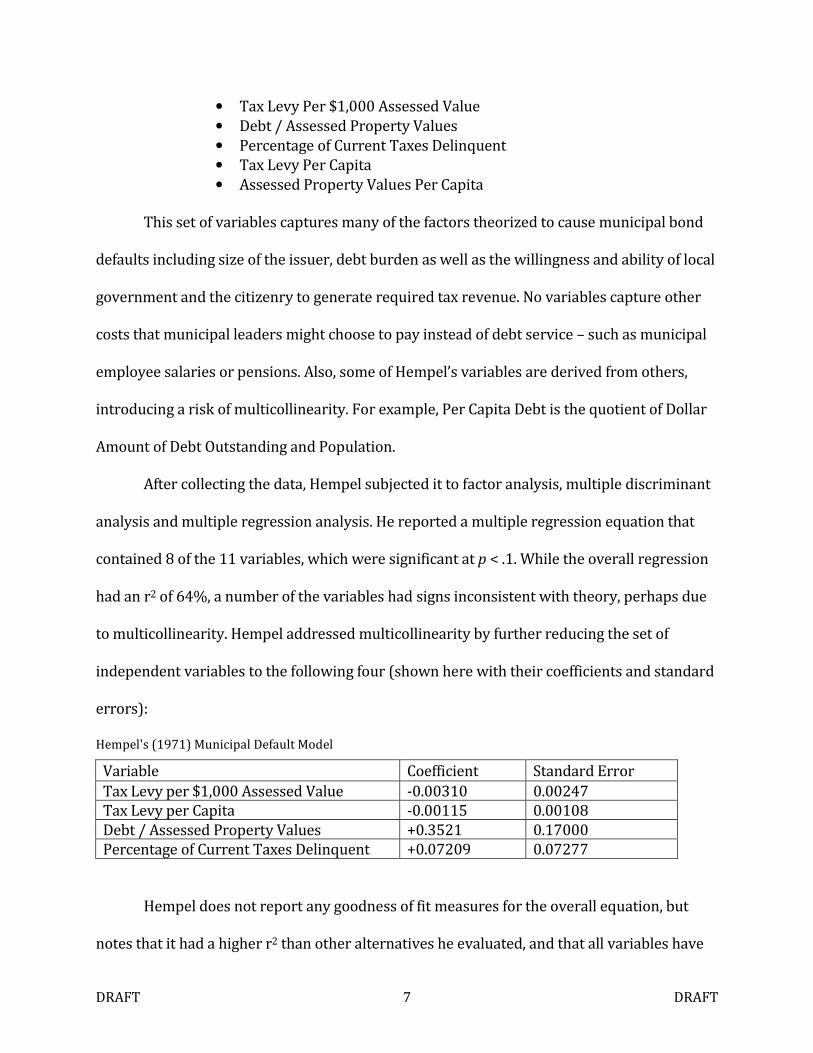
to multicollinearity. Hempel addressed multicollinearity by further reducing the set of
independent variables to the following four (shown here with their coefficients and standard
errors):
Hempel's (1971) Municipal Default Model
Variable Coefficient Standard Error
Tax Levy per $1,000 Assessed Value -0.00310 0.00247
Tax Levy per Capita -0.00115 0.00108
Debt / Assessed Property Values +0.3521 0.17000
Percentage of Current Taxes Delinquent +0.07209 0.07277
Hempel does not report any goodness of fit measures for the overall equation, but
notes that it had a higher r2 than other alternatives he evaluated, and that all variables have
DRAFT 8 DRAFT
the expected sign. On the other hand, two of the four variables are not significant at p < .05,
while the two best predictors are theoretically related.
In the interest of using Depression-era data to predict future defaults, it is fortunate
that certain variables fell out of Hempel’s specification. Given the substantial change in prices
and wealth since the 1930s, it would be difficult to use the Dollar Value of Notes Outstanding,
the Dollar Value of Debt Outstanding or Per Capita Debt to model current issuers. Tax Levy
per Capita, which remained in Hempel’s specification, has a similar challenge. Variables that
take the form of ratios, such as Debt/Assessed Property Values or Tax Levy per $1000
Assessed Value are more appropriate for analysis and forecasting independent of time
period.
Hempel (1973) later expanded the sample to 45 Michigan cities – 28 of which
defaulted – and 23 independent variables. Many of the added variables were 1922 values
most likely obtained from that year’s Census of State and Local Governments. He identified a
regression equation with nine exogenous variables significant at p < .05.
Hempel's (1973) Municipal Default Model
Variable Coefficient Standard Error
Log of 1932 Population -0.07678 0.0321
Assessed Property Value Per Capita in 1932 +0.0001585 0.0000523
Growth of Population from 1922 to 1932 -0.02146 0.0113
Growth of Debt Relative to Population Growth -0.007912 0.00213
Debt/Assessed Property Values in 1932 +0.4885 0.258
Tax Levy Per $1000 Assessed Value in 1932 +0.00919 0.00242
Tax Levy Per Capita in 1932 -0.007197 0.00322
Percentage of Current Taxes Delinquent in 1932
+0.2095 0.0962
Notes Outstanding Per Capita in 1932 +0.009159 0.00246
Hempel noted the presence of multicollinearity but did not present an alternative
equation that addressed it. Two of the nine variables presented above – Growth of Debt
DRAFT 9 DRAFT
Relative to Population Growth and Tax Levy Per Capita in 1932 – have coefficient signs that
are inconsistent with intuition. Hempel reported that the nine variable regression had an
adjusted r2 of 51%, while alternatives that remedied multicollinearity had adjusted r2 of
between 39% and 45%.
In his discussion of Hempel’s findings, Forbes (1973) questions the use of Depression-
era data for modeling purposes, while admitting that the paucity of more recent defaults
forces this choice. In particular he noted that local governments received more state aid – at
the time of his writing – than they did in the 1930s. This institutional change could reduce
the relevance of the historic default data.
Predicting Credit Ratings as a Proxy for Estimating Default Risk
Rubinfeld (1973) proposed a multiple regression model for predicting credit ratings.
Since credit ratings are intended to convey information about the likelihood of default,
exogenous variables that explain credit ratings could also be used as predictors of default.
Using a sample of 128 New England municipal bond issuers, he found that the following
independent variables were predictive of the credit rating at the 10% significance level:
• Percentage of Taxes Uncollected in the Previous Year
• Ratio of Direct Net Debt to Assessed Valuation
• Median Family Income
• Full Valuation of the Property Tax Base
• Overlapping Debt
The first two of these exogenous variables are consistent with those in Hempel’s 1973
study. Overlapping Debt refers to the indebtedness of other issuers who rely on the same tax
base. For example, if property owners pay taxes to both their city and county and if both
governmental entities carry debt, the county’s debt would be considered overlapping debt
DRAFT 10 DRAFT
viz.-a-viz. the city and vice versa. This variable, along with Median Family Income and Full
Valuation of the Property Tax Base, would have to be restated as a ratio to be useful in a
default prediction model.
Carelton & Lerner (1969) attempted to use statistical techniques to match Moody’s
bond ratings using a random sampling of issuers extracted from Moody’s 1967 Municipal
and Government Bond manual. They tested six variables – all of which they found to be
significant. These were:
• Whether the issuer was a School District
• Ratio of Debt to Assessed Valuation
• Ratio of Debt to Population
• Log of Population
• Log of Debt
• Average Collection Rate
Using a large sample of 976 cities, Farnham & Cluff (1984) tested 23 variables to
determine whether they were predictive of Moody’s bond ratings. They found 12 of the
variables to be significant α = .05. The method used was an “N-chotomous” probit analysis.
The authors chose this method because the four possible ratings in the dependent variable
were thought to be of unequal lengths, i.e. many more cities fell into the A rating category
than into the Aaa category. Their analysis included several variables not considered by other
authors – including housing stock attributes, form of government and geographical location.
Four of the housing stock attributes proved to be significant. Farnham & Cluff’s variables are
listed in the following table.
DRAFT 11 DRAFT
Farnham & Cluff's (1984) Independent Variables
Variable Significant at 5% Level?
Gross Debt / 1000 Population *
Total General Revenue *
Percent Change in Total Revenue *
Assessed Valuation *
Population
Percent Change in Population
Percent Nonwhite *
Percent Eighteen Years and Under
Population Density *
Income Per Capita
Ratio of Non-Workers to Workers *
Number of Manufacturing Establishments
Percent One-Unit Housing Structures *
Percent Housing Units Occupied
Percent Housing Units Owner Occupied *
Percent Housing Units Built Before 1940 (as of 1970) *
Median Value of Owner Occupied Housing Units *
Median Years of Education *
Local Documents Available
Council-Manager Form of Government
City Located in Northeast Region
City Located in Northcentral Region
City Located in South
The papers reviewed above are part of a large literature that attempts to estimate
municipal bond ratings. Loviscek & Crowley (1990) compare the studies described here with
eleven others that had the same objective.
Since Loviscek & Crowley published their review, at least two additional papers
modeling municipal bond ratings have appeared. Moon & Stotsky (1993) analyzed data for
892 US cities with population over 25,000, of which 727 were rated. They first modeled the
decision by city officials to seek a rating and then factors determining the ratings actually
DRAFT 12 DRAFT
assigned. This methodology highlights the fact that by choosing to be rated, cities self-select
into the samples used in previous studies. This suggests that studies which use ratings as a
proxy for default probability suffer from selection bias.
Moon & Stotsky (1993) found that cities choosing to remain unrated were likely to
receive a low rating. They tested twenty variables potentially affecting rating levels, and
found 15 to be significant. The variables they evaluated were as follows:
Moon & Stotsky's (1993) Independent Variables
Variable Significant at 5% Level?
Median Housing Value *
Proportion of Housing Units that were Built Before 1940 *
Proportion of Housing Units that were Built After 1970
Proportion of Housing Units that are Owner-Occupied *
Per Capita income *
Percentage Change in Population from 1970 to 1980 *
Proportion of the Population that is Non-White *
Population Density *
Total Debt
Per Capita Debt *
Ratio of Debt to Income *
Ratio of Surplus Revenues to General Revenues
Ratio of Intergovernmental Revenues to General Revenues
Council-Manager form of government *
Commission Form of Government
City Located in Midwest *
City Located in South *
City Located in West *
Population Between 100,000 and 500,000 *
Population Greater Than 500,000 *
Most recently, Palumbo & Zaporowski (2012) analyzed ratings for 965 county and
city governments rated by Moody’s in 2002. This population encompassed all such units that
issued rated full faith and credit debt and that could be matched against Census, Bureau of
DRAFT 13 DRAFT
Economic Analysis (BEA) and Bureau of Labor Statistics (BLS) data sets. Of the 15 variables
they examined, 13 proved to be significant at the 5% level as shown below.
Palumbo & Zaporowski's (2012) Variables
Variable Significant at 5% Level?
Per Capita Income *
Percentage Change in Population 1990-2000 *
Unemployment Rate *
Percentage Change in Earnings Per Worker 1986-2001 *
Economic Diversity Index from BEA *
State Aid Per Capita *
State General Obligation Bond Rating *
Debt to Market Value (Ratio of Full Faith and Credit Debt to Population Weighted Median Value of Housing) *
Non-Guaranteed Debt Per Capita
Per Capita Interest Payments for Nonutility Debt
Per Capita General Revenues *
State Imposed Taxation Limit *
State Imposed Expenditure Limit *
Objections to Rating Based Analysis
Researchers who model ratings rather than defaults, implicitly assume that the
former predict the latter.1 However, if ratings do not change in response to underlying credit
conditions experienced by municipal bond issuers, they may not be an effective proxy for
default risk. Under SEC rules, rating agencies are required to publish transition matrices
showing the distribution of rating changes over a given period. A review of the transition
matrices published by Moody’s Corporation (2012), Standard & Poors Corporation (2012a)
1 In fairness to the authors of these studies, it is worth pointing out that most do not make the claim that ratings
proxy default probability. When modeling credit ratings, researchers may have goals other than estimating default
probability. For example, they may be interested in modeling rating agency behavior.
DRAFT 14 DRAFT
and Fitch, Inc. (2012) suggests that about 90% of municipal bond ratings remain unchanged
within a given year.
For example, an S&P transition matrix (for non-housing municipal issuers) shows that
89.11% of AA rated issuers remained AA the following year, while 0.18% were upgraded to
AAA, 1.62% were upgraded to AA+ and a total of 9.09% were downgraded to various rating
categories ranging from AA- down to BB+.
The S&P matrix represents all rating change activity that occurred between 1986 and
2011. During most of this period, a substantial proportion of municipal bond ratings
reflected insurance “enhancements”. So-called monoline insurers like Ambac, FGIC and MBIA
– which were rated AAA – sold bond insurance policies to municipalities guaranteeing that
any missed bond payments would be covered by the insurer. Consequently, the ratings
assigned to these insured issuers were AAA – reflecting the estimated credit quality of the
insurer. During the 2007-2008 financial crisis, all monoline bond insurers went out of
business or suffered ratings downgrades (Palumbo & Zaporowski, 2012).
While the insurance was in place, ratings might have appeared to remain stable
despite changes in municipal credit conditions, simply due to the stability of the insurer’s
credit rating. However, Fitch’s NRSRO ratings transition exhibit states that the ratings
analyzed are “unenhanced” which means they reflect the underlying credit quality of the
issuer excluding any insurance benefit. We expect that that is also the case for the S&P and
Moody’s tables.
Insurance coverage aside, municipal ratings stability could be explained by some
combination of three factors. First, underlying credit conditions for most issuers do not
materially change from year to year. Second, ratings grades are too coarse to capture many
DRAFT 15 DRAFT
credit quality changes. And, third, rating agencies do not perform sufficient surveillance
activities to detect and respond to many changes in issuer credit quality. To the extent that
the second and third causes are explanatory, they pose challenges to the use of ratings as a
proxy for default probability.
Little evidence is available to determine the relative weight of each of these three
factors. One item that may be relevant is the criticism rating agencies received for their
inadequate monitoring of Residential Mortgage Backed Securities (RMBS) and Collateralized
Debt Obligations (CDO) prior to the financial crisis of 2007 and 2008. The United States
Senate Permanent Subcommittee on Investigations (2011) found that:
Resource shortages impacted the ability of the credit rating agencies to conduct
surveillance on outstanding rated RMBS and CDO securities to evaluate their credit risk.
The credit rating agencies were contractually obligated to monitor the accuracy of the
ratings they issued over the life of the rated transactions. CRA surveillance analysts were
supposed to evaluate each rating on an ongoing basis to determine whether the rating
should be affirmed, upgraded, or downgraded. To support this analysis, both companies
collected substantial annual surveillance fees from the issuers of the financial
instruments they rated, and set up surveillance groups to review the ratings. In the case
of RMBS and CDO securities, the Subcommittee investigation found evidence that these
surveillance groups may have lacked the resources to properly monitor the thousands of
rated products. At Moody’s, for example, a 2007 email message disclosed that about 26
surveillance analysts were responsible for tracking over 13,000 rated CDO securities. (p.
314).
Since these findings relate to structured securities rather than municipal bonds, it is
possible that they are not relevant. On the other hand, it is reasonable to think that if rating
companies under-invested in surveillance for their most profitable asset class – structured
finance - (Cornaggia, Cornaggia & Hund, 2011), they probably made similar under-
DRAFT 16 DRAFT
investments in the surveillance of other asset classes. It is the co-author’s contention, - based
on his experiences at a major rating agency - that surveillance procedures for structured
assets were actually superior to those undertaken for municipal bonds.
Estimating Default Probability from Market Prices
A number of researchers have attempted to derive default probabilities from bond
yields or Credit Default Swap (CDS) spreads (Longstaff, Mithal & Neis, 2004). In theory, bond
yields should be a function of their credit risk. More specifically, yields should compensate
investors for the expected loss arising from a potential default. In the literature, expected loss
is defined as the product of default probability and loss given default (LGD). LGD is simply
the complement of a bond’s rate of recovery, and is also called “loss severity”.
Theoretical bond yields contain a number of components aside from expected loss.
Bohn, Arora and Agarwal (2004) propose an equation for corporate bond yields that includes
the risk free rate of interest, the level of investor aversion to risk, the bond’s maturity date,
issuer size (as a proxy for liquidity) and the correlation of the bond’s default risk with that of
other instruments. Yields may also be affected by call provisions that give issuers the option
to redeem their bonds prior to maturity.
With respect to municipal bonds, a further complexity arises as a result of their tax
status. Since interest on most municipal bonds is exempt from federal, state and local income
taxation, their yields are not comparable to those on taxable securities. Some adjustment to
the municipal bond yield must be made in order to make it “taxable equivalent”. One
approach is to convert the tax free yield to a taxable yield based on the highest prevailing
marginal tax rate, on the assumption that municipal investors are predominantly high
income individuals. However, given the complexities of the tax code, the heterogeneity of
DRAFT 17 DRAFT
individual investors and the participation of institutional investors (with different tax
considerations), the use of the top marginal rate is a relatively strong assumption. Chalmers
(1998) finds that interest rate differentials between long term US Treasuries and federally
insured municipals (which are assumed to have no default risk) are not consistent with the
tax benefits available to individuals in the top tax bracket.
The literature includes a number of efforts to decompose municipal bond yields into
default risk and other components. Wu (1991) found that the risk aversion factor was not
significant, but his functional form excluded recovery rates. Wu, Wang & Zhang (2006)
offered a more comprehensive model that included a static recovery rate assumption. The
authors attributed a substantial portion of municipal bond yields to liquidity factors.
In corporate credit markets, analysts often derive default probabilities from CDS
spreads rather than bond yields. Credit Default Swaps are insurance contracts against
default. If the issuer defaults, the CDS seller (or insurer) pays the protection buyer the face
value of the bond and takes the bond in exchange. Deriving default probabilities from CDS
spreads is easier than using bond yields because CDS have fewer complexities, such as call
provisions. The applicability of CDS implied default probabilities to the municipal market is
greatly limited, however, by the fact that CDS trades against a relatively small number of
municipal issuers, and trading volume is low even for those issuers for which CDS are
available.
A final concern regarding market implied default probabilities pertains to how
efficiently markets price credit risk. Decomposing yields into default probabilities and other
components implicitly assumes that bond prices are efficient, i.e. that they accurately reflect
all available information. This assumption is consistent with the strong form of the Efficient
DRAFT 18 DRAFT
Markets Hypothesis (EMH) markets advanced by Fama (1970). More recently EMH
generally, and the strong form of the hypothesis in particular, have come under attack
(Summers, 1986; Crotty, 2011). Most tests of EMH have involved equities rather than bonds.
In a 2003 survey of EMH literature, Malkiel (2003) identified only one study addressing bond
market efficiency, and that paper found inefficiency in the pricing of corporate bonds (Keim
& Stambaugh, 1986). Since large capitalization stocks experience much higher trading
volumes than municipal bonds, it is not clear that EMH applies at all to the latter asset class.
Indeed, there is a substantial literature documenting the lack of liquidity and transparency in
the municipal bond market – suggesting the existence of substantial inefficiencies (Ang &
Greene. 2011).
In summary, the task of deriving default probabilities from municipal bond yields is
impeded by both the complexities of decomposing yields into their components and the
likelihood that observed yields do not efficiently incorporate credit risk insight.
Default Probability Modeling Using Logit and Probit Techniques
More recent efforts to model bond default probabilities have used logit and probit
techniques. An obvious advantage of logit and probit over Ordinary Least Squares (OLS) for
default probability modeling is that the dependent variable is restricted to a range of 0 to 1.
In addition, the use of a binary endogenous variable, like default/non-default, violates a
number of assumptions of the OLS model. (Menard, 2002).
Because corporate bankruptcy has been much more common than municipal default,
the academic literature contains many more efforts to model the former. Ohlson (1980) was
first to apply a logit model to corporate bankruptcy modeling.
DRAFT 19 DRAFT
Shumway (2001) built upon previous logit models by using panel rather than cross
sectional data. This approach addresses the fact that most bankrupt firms were solvent for
many years before going into distress, and that it is thus useful to analyze a time series of
data for each firm.
The literature also contains applications of probit models to corporate bankruptcy
starting with Zmijewski (1984). Moody’s RiskCalc is a commercial private firm default
probability model that uses probit. The RiskCalc methodology document written by
Falkenstein, Boral & Carty (2000) suggests that the choice of probit over logit was not a
significant one, as the two models usually produce similar results. On the other hand, Altman
& Sabato (2007) assert that logit models have outperformed probit models in the corporate
bankruptcy field.
Probit and logit models are functionally similar, with the key difference being the fact
that probit is based on a cumulative normal probability density function, whereas logit uses a
logarithmic distribution. This latter distribution has more observations in its left and right
tails and fewer observations at its center. Ameniya (1980), in his extensive survey of binary
choice and other discrete choice models concludes that “it does not matter much whether
one uses a probit model or a logit model, except in cases where data are heavily
concentrated in the tails due to the characteristics of the problem being studied (p. 1487).”
Although the published literature does not appear to include general obligation
municipal bond default probability models that employ logit and probit techniques,
Bialaszewski (1985) applied a logit model to a set of municipal revenue bonds – issues which
are supported by user fees and other operating revenues collected by the issuing agency
rather than with tax revenues. Bialaszewski collected financial, economic and demographic
DRAFT 20 DRAFT
data for 36 defaulted revenue bonds and for 36 comparable bonds that did not default. She
then created models using data at issuance, two years prior to default, one year prior to
default and at the time of default. Different variables were significant in each model. She
reported that her one year prior to default model accurately classified 87% of the
observations into defaulting and non-defaulting categories, where these categories were
defined in terms of a “cut point” in the calculated probabilities. Her cut point of 65.8% was
set to produce the highest degree of accurate classification. It may be more appropriate to
use a fixed cut point of 50%, since probability estimates over that level could be reasonably
characterized as default predictions, while probabilities under this level could be seen as
predictions of non-default. The significant variables in Bialaszewski’s regression were: (1)
Total Population, (2) Percentage of Population that is Non-White, (3) Debt Service as a
Percentage of Total Revenue, (4) Welfare Payments as a Percentage of Total Revenue and (5)
Short Term Debt as a Percentage of Cash and Security Holdings.
Since the observations involved revenue bonds, the theoretical case for some of the
variables in this specification is not immediately apparent. For example, welfare payments
are financed by a municipality’s general fund, and should thus not be expected to compete
with revenue bondholders for priority. On the other hand, non-white population and welfare
dependency levels may be indicators of poverty. Impoverished residents may be less able to
pay fees required to service debt incurred by the facilities that defaulted.
Finally, the use of race-based criteria for evaluating municipal bonds has been subject
to criticism. Yinger (2010) finds that general obligation municipal bond ratings penalize
communities with relatively high non-white populations despite the lack of evidence that

DRAFT 21 DRAFT
these communities are more likely to default. He characterizes this result as a form of
redlining and argues for municipal bond rating regulation to curtail this practice.
DRAFT 22 DRAFT
Great Depression Review and Analysis2
Since 1940, interest or principal payment defaults on US municipal bonds have been
rare. This is especially true of general obligations bonds – those backed by the full faith and
credit of a state, county, city or other governmental unit with taxing authority. By contrast,
there were about 4800 reported municipal bond defaults during the 1930s (ACIR 1973;
Fons, Randazzo & Joffe, 2011).
With the assistance of colleagues and a data entry vendor, Joffe (2012) collected
information on approximately 5000 defaults from the period 1920 to 1939. The primary
sources were contemporary Moody’s Municipal and Government Bond Manuals (now
published and owned by Mergent Corporation), and back issues of the Daily Bond Buyer and
weekly Bond Buyer. Joffe (2012) also found and catalogued defaults from state-level bond
listings and other documents housed in state archives, Reconstruction Finance Corporation
records, local newspaper accounts and other sources.
In their book, This Time is Different, Carmen Reinhart and Kenneth Rogoff (2009)
marshaled older data in their analysis of banking and sovereign debt crises. Due to the
paucity of recent defaults, a similar approach may be applicable to US municipal bonds. In
contrast to some areas of fixed income - such as mortgage backed securities - institutional
change in the municipal sphere over the last century has been incremental rather than
revolutionary. Political and budgetary processes at the state and local level have evolved
relatively slowly in the context of a stable national political framework. Older municipal
2 This section contains previously published research that originally appeared in Fons, Randazzo and Joffe (2011)
and Joffe (2012). However the statistical analysis presented below has been updated for this report.
DRAFT 23 DRAFT
defaults are thus more relevant to modern experience than older defaults in other asset
classes.
The goal of this chapter is to mine the Depression-era municipal bond default record
to learn whatever insights it can offer for present day credit research. This is done by
providing a brief description of the 1930s municipal credit crisis and by developing a
quantitative default probability model.
The Depression Era Municipal Default Wave
According to US Treasury statistics reported by The Bond Buyer, the dollar volume of
municipal bonds outstanding more than quadrupled between 1913 and 1931 – a period
during which the CPI rose 54%. The boom in municipal issuance during this period is largely
attributable to the inception of the federal income tax and the popularization of automobile
travel. Municipal bond interest was exempt from income taxes since the levy’s 1913
inception, creating demand for these securities among high income investors. On the supply
side, automobiles created a need for paved roads – which states, counties and cities often
financed with bonds. Communities also used bonds to finance drainage, irrigation and levee
projects to support agricultural developments and to fund school construction.
Those concerned about today’s municipal credit quality correctly point to the rapid
growth in municipal bonds outstanding in recent years. But the growth in municipal bonds
outstanding between 1913 and 1931 far exceeded the rate of increase over the eighteen
years up to 2010 – and both of these booms were outpaced by growth following World War
II, during the years 1946 to 1964. While the pre-Depression municipal bond boom ended
with a spike in defaults, the post-War expansion was not followed by a similar circumstance.
DRAFT 24 DRAFT
Bank Closings, Bank Holidays and Municipal Bond Defaults
It is also worth considering that the peak in estimated municipal default rates
coincided with a nationwide outbreak of bank failures and bank holidays. In a 1933 survey of
1,241 state, city and county financial officials, Martin Faust (1934, 1936) found that slightly
more than half of their governmental units had funds in closed banks. The municipalities
surveyed had a total of over $98 million tied up in these failed institutions. Faust estimates
that the aggregate balance in failed banks for all state and local governments would have
been $450 million – more than 2% of the principal outstanding on municipal bonds at the
time. Contemporary accounts attributed many of the defaults to the closure of banks in
which funds intended for bondholders had been deposited.
A major source of distress for municipalities in North Carolina, Louisiana, Arkansas,
Tennessee and other southern states was the November 1930 collapse of Caldwell &
Company and its affiliates. Founder Rogers Caldwell, dubbed the “J.P. Morgan of the South”
had built a large business marketing municipal bonds issued by southern states. Bond
proceeds were typically held at Caldwell’s Bank of Tennessee until they were required by the
issuer. According to John McFerrin’s (1939) history of Caldwell and Company, most issuers
required that their deposits be supported by high quality collateral – typically other
municipal bonds. Caldwell often pledged such bonds as collateral initially, and then
substituted illiquid, high-risk real estate bonds without notifying the issuer. In addition to
following deceptive practices, Caldwell looted bank assets to finance an extravagant lifestyle.
On November 7, 1930, a Tennessee state audit declared Caldwell & Company
insolvent. News of this declaration triggered runs on Caldwell and numerous affiliated banks
throughout the South. In Tennessee alone, $9 million in county and municipal deposits were
DRAFT 25 DRAFT
lost. Caldwell’s failure triggered a run on affiliates, including Central Bank and Trust
Company in Asheville, North Carolina, which was followed by runs on other area banks.
Property Tax Delinquencies
While the vast majority of the enumerated defaults occurred in special districts,
school districts and small towns, the Depression-era did witness several spectacular defaults
by large issuers including Cleveland and Detroit. New York City, the nation’s largest
municipality back then, also experienced a brief default in December 1933. Chicago, then the
nation’s second largest city, narrowly avoided default by refinancing its bonds at lower
interest rates. Cook County – which encompasses the city – failed to make scheduled interest
and principal payments, as did a number of independent taxing districts within the city’s
limits.
As statistics collected at the time by Dun & Bradstreet (Bird, 1936) suggest, major city
defaults during the Great Depression were preceded by substantial spikes in tax delinquency
rates. For example, the tax delinquency rate in Detroit rose from 10.8% in fiscal year 1930 to
17.2% in 1931, 25.0% in 1932 and 34.8% in 1933 – the year in which it defaulted. In New
York and Chicago, delinquency rates peaked at 26.5% and 42.4% respectively.
Although many of the property tax delinquencies were undoubtedly the result of
economic distress, the early 1930s was also a period of organized tax revolts. This long-
forgotten tax resistance movement is described in David Beito’s 1989 book Taxpayers in
Revolt. Beito argues that the resistance was in large measure a reaction to substantial
increases in property taxes during the preceding decade. This increased burden was often
accompanied by stable or falling property values, since the 1920s was a time of weak real
estate prices.
DRAFT 26 DRAFT
Beito traces the history of the property tax resistance movement in Chicago where
anti-tax activism was most potent. The Chicago resistance was led by the Association of Real
Estate Taxpayers (ARET), an organization originally formed by relatively affluent investors,
but which later attracted broad support among the City’s skilled blue collar workers worried
about maintaining their foothold in the middle class. At its peak, ARET leaders hosted a
thrice-weekly radio program and the organization had 30,000 members.
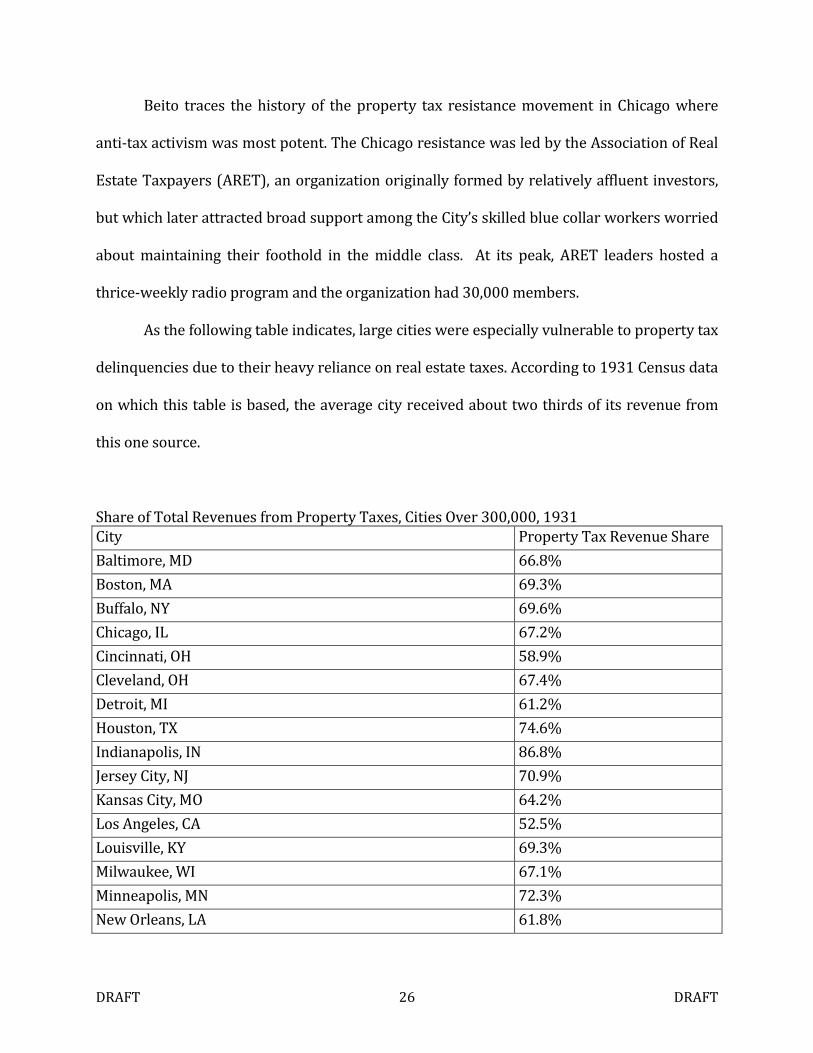
As the following table indicates, large cities were especially vulnerable to property tax
delinquencies due to their heavy reliance on real estate taxes. According to 1931 Census data
on which this table is based, the average city received about two thirds of its revenue from
this one source.
Share of Total Revenues from Property Taxes, Cities Over 300,000, 1931
City Property Tax Revenue Share
Baltimore, MD 66.8%
Boston, MA 69.3%
Buffalo, NY 69.6%
Chicago, IL 67.2%
Cincinnati, OH 58.9%
Cleveland, OH 67.4%
Detroit, MI 61.2%
Houston, TX 74.6%
Indianapolis, IN 86.8%
Jersey City, NJ 70.9%
Kansas City, MO 64.2%
Los Angeles, CA 52.5%
Louisville, KY 69.3%
Milwaukee, WI 67.1%
Minneapolis, MN 72.3%
New Orleans, LA 61.8%
DRAFT 27 DRAFT
City Property Tax Revenue Share
New York, NY 70.8%
Newark, NJ 69.1%
Philadelphia, PA 71.8%
Pittsburgh, PA 81.2%
Portland, OR 65.7%
Rochester, NY 66.5%
San Francisco, CA 59.5%
Seattle, WA 47.5%
St. Louis, MO 62.5%
Washington, DC 56.1%
While over-reliance on one revenue source can be attributed to the relative lack of
municipal finance sophistication at the time, part of the problem was beyond the control of
city governments. According to Census statistics reported by C. E. Rightor (1938) in
Municipal Finance, roughly 4-1/2% of major city revenue was derived from alcohol taxation
in 1916. This revenue source disappeared with Prohibition, and did not return until the 18th
Amendment was repealed in 1933. Additional policing costs associated with Prohibition-
related organized crime must have further contributed to the cities’ fiscal distress.
Public Employee Pensions
Contemporary concerns about municipal bond defaults are often linked to public
pensions, but underfunding is not unique to our era. During the Great Depression, many
retired government workers were eligible for pensions. Buck (1936) notes that before the
establishment of pensions, older municipal employees would continue to report for work
even though they could no longer perform their jobs (at least not to the satisfaction of
contemporary management). Supervisors, guided by a humanitarian impulse rather than a
DRAFT 28 DRAFT
concern for the bottom line, were reluctant to fire these older employees. Administrators
thus reached the conclusion that it would be less expensive to pension off the older workers
at a percentage of their former salary.
Many cities had not yet created pension funds and those that did often failed to make
actuarially appropriate contributions. A 1937 National Municipal League Consulting Service
survey of Atlanta’s finances reported serious underfunding in the city’s three pension funds: .
It is obvious from these figures that the firemen's fund with a cash balance of $491.38
is no fund at all. Nor are the reserves of either the general or police funds even a faint
approximation of what they should be to guarantee the payment from the fund of its
probable obligations. ... Firemen this year who paid money into their pension fund saw
it go out again immediately to pay other firemen's pensions. Their sacrifice in no way
built up for them any protection. They have in fact nothing to rely on but the naked
promise of the city as their security for old age. We would recommend therefore that in
all the pension funds the employee's contribution be treated as a trust fund and
invested for him in securities or in the purchase of an annuity.
That said, the NML consultants were not advocates of full funding:
We believe on the other hand that it is not necessary for a public body deriving its
income from taxes to accumulate a fund as if it were a private insurance company.
Unless there are some predictable sharp upturns in the curve of natural retirement
there is no reason why the City should not pay pensions out of income. The integrity
and solvency of the city should be a sufficient guarantee to the employee that the city
will fulfill its pension contract. In fact if the city went bankrupt any fund it might have
accumulated would probably disappear in the crash.
Atlanta public employee pensions at the time were generous – at least by the
standards of today’s private sector. Employees could retire on 50% of their salary after 25
years of service, regardless of age. Survivor benefits were also provided. Atlanta avoided
default during the Depression and evidence reviewed thus far does not attribute any case of
DRAFT 29 DRAFT
municipal default during the 1920-1939 timeframe to employee pensions. Although pensions
were available to Depression-era public employees, legal protections for these benefits have
increased in recent decades. It may be appropriate to conclude that pension benefits were
junior to debt service in a government’s priority of payments during the 1930s, while today
these two types of obligation appear to be almost pari passu, that is, on equal footing.
Data Selection
Today, the municipal bond market covers a broad range of issuers. This diversity was
also present – albeit to a lesser extent – in the years prior to World War II. The municipal
bond default list compiled in Joffe (2012) includes 5079 issuers who failed to make timely
and complete principal or interest payments (or who obliged investors to accept refunding
bonds in lieu of cash at maturity) at some time between 1920 and 1939. Most of the
defaulting issuers were school districts, small towns and special tax districts – created to
build roads and other infrastructure.
Financial data for special assessment districts and for school districts is more limited
than for other issuer categories. Moody’s bond manuals provide some data, but it is
incomplete and not in a consistent format. The best data is available for states and large cities
because they reported their financial statistics to annual Censuses at the time.
Comprehensive financial data for smaller cities and counties was collected by decennial
Censuses in 1922 and 1932.
Since annual Census data is available for a substantial number of larger cities, and
since these cities experienced a significant number of defaults, the statistical analysis is most
readily applicable to this subset of issuers.
DRAFT 30 DRAFT
For fiscal years 1930 and 1931, the Census Bureau reported financial statistics for
311 US cities with population over 30,000 (as of April 1, 1930). After 1931, the collection
effort was scaled back, perhaps due to budgetary pressures at the federal level. In fiscal years
1932 and 1933, the Bureau reported similar statistics for 94 cities with population over
100,000 (also as of April 1, 1930). In fiscal 1934, Honolulu was added to the annual data set.
Thus annual time series of fiscal data are available from the Census for 94 cities during the
Depression period while more limited data is available for an additional 217 cities. In all, a
total of 1000 city/year observations are available for the period FY 1930-1935. Data
reported for each entity include revenues by category, expenditures by category, as well as
various classifications of assets and debt.
Of the 311 cities in the sample, 46 had defaults on general obligation bonds between
1930 and 1936, implying a cumulative default rate of 15% for this sample. The overall
municipal default rate during this period was about 16%. Among the non-defaulting cities,
some had “forced refundings” in which investors were obliged to exchange maturing bonds
for new ones with later maturities. Many others had defaults on special assessment bonds
which were not general obligations of the cities. In the following analysis, none of these
instances are classified as a default – but adjusting the default classifications in light of these
circumstances is a reasonable task for future research.
Some defaults were attributed at the time to bank closures or bank holidays. Since
FDIC insurance is now available, it would be reasonable to exclude defaults that really were
the result of banking issues. However, reclassifying such defaults should only be done after
an intensive reading of contemporary newspapers to confirm that they were fully
attributable to banking problems. In certain cases, city officials may have used bank closures
DRAFT 31 DRAFT
or holidays as a pretext to obscure fiscal problems that rendered the city unable or unwilling
to pay even if funds had not been temporarily frozen. Thus, these classification adjustments
are also left to future research.
Once a city defaults, its data may become idiosyncratic as it suspends interest
payments and possibly writes down principal. For example, Miami’s interest costs fell from
$2.2 million in 1929 to $0.3 million in 1933. News sources indicate that the city first
defaulted in 1930. Since the purpose of the analysis is to predict default, post-default
observations are dropped from the data set, resulting in the loss of 43 observations. Of the
remaining 957 city/year pairs in the sample, 125 are associated with defaulting cities.
Although several hundred series are available in the Census data, most of them relate
to small components of revenue and expenditure. This still leaves a number of aggregate
revenue, expenditure, debt and asset series that may yield useful explanatory variables.
Below, variables are evaluated in ratio form to maximize their modern relevance despite the
substantial increase in population, price levels and per capita economic output that have
occurred over the last 80 years.
Conceptual Model and Variable Selection
The ratio most commonly used in discussions of sovereign credit is the debt-to-GDP
ratio, and that concept is sometimes applied to lower levels of government. The fiscal Census
data do not include GDP or any other indicia of economic activity. More recently, regional
income account statistics have been reported for states, metropolitan areas and counties in
recent years, but most series do not extend back to the Depression era.
Although reliable measures of total economic output are not available at the
municipal level, other demographic and macroeconomic variables can be employed. Previous
DRAFT 32 DRAFT
studies have used population, assessed valuation and per capita income as independent
variables in default probability or rating prediction models.
Given fiscal data is available, the use of demographic and macroeconomic variables
may not be necessary. The choice of whether to pay or default upon debt service obligations
is made by the political leaders of a governing unit. The most immediately accessible data
available to these officials include the size of the interest or principal payment that needs to
be made, what financial resources are available to the government to make the payment and
what other spending priorities are competing with the debt service obligation.
Consequently, the model constructed here is derived solely from fiscal measures. We present
several alternative models in Appendix 1 that do include socioeconomic variables. The
models presented in the Appendix 1are also subjected to alternate specifications and
estimation strategies as checks on the robustness of the results presented here.
Rating agencies use a number of purely fiscal metrics that can be estimated directly
from the municipal Census data set. One commonly used metric is the ratio of interest costs
to revenue. The rationale for including this ratio is that a default becomes likely when
interest costs become so onerous that they threaten to crowd out other spending priorities.
When the interest burden is low, it is not rational for a political leader to default, because he
or she then loses access to capital markets and is thus compelled to reduce spending or raise
taxes. As interest expenses rise, this disincentive is increasingly likely to be outweighed by
the near term political costs of cutting spending on popular programs.
This theoretical underpinning does have a couple of limitations that should be noted.
First, defaults often occur when a principal payment – rather than an interest payment –
becomes due. In the Depression era, cities were more vulnerable to principal repayment
DRAFT 33 DRAFT
defaults because the concept of serialized maturities had yet to become popular. Large bond
issues were typically scheduled to mature all at once. Many obligors accumulated revenues in
“sinking funds” to meet these large debt repayments, while others expected to pay off the
maturing bonds by issuing new ones. When sinking fund assets declined in value and the
new issue market dried up, many governments were unable to redeem or roll over maturing
issues. In the aftermath of the Depression experience, public finance specialists began to
advocate serialized maturities, under which a large bond issue is broken down into a number
of smaller tranches whose principal becomes due at varying dates – often one year apart.
Second, revenue may not be an ideal denominator, since political leaders may have
the option of running surpluses or deficits. While many state and local governments are and
have been subject to balanced budget requirements, these are typically prospective rather
than retrospective and are often subject to evasion. On the other hand, using expenditures
rather than revenues as a denominator is also an imperfect measure. Local governments
cannot sustain large annual deficits indefinitely, so revenues appear to be a better indicator
of their long term fiscal capacity.
A review of the 957 city/year observations shows that defaulting cities tended to have
higher interest to revenue ratios than those that did not default. This is reflected in the box
and whisker plot below. Further, a one sided t test of the defaulting and non-defaulting
sample means fails to reject the null hypothesis that defaulting cities have higher interest to
revenue ratios than non-defaulting cities at p < .0001. The sample mean for defaulting cities
is 16.1% versus 11.0% for cities that did not default.
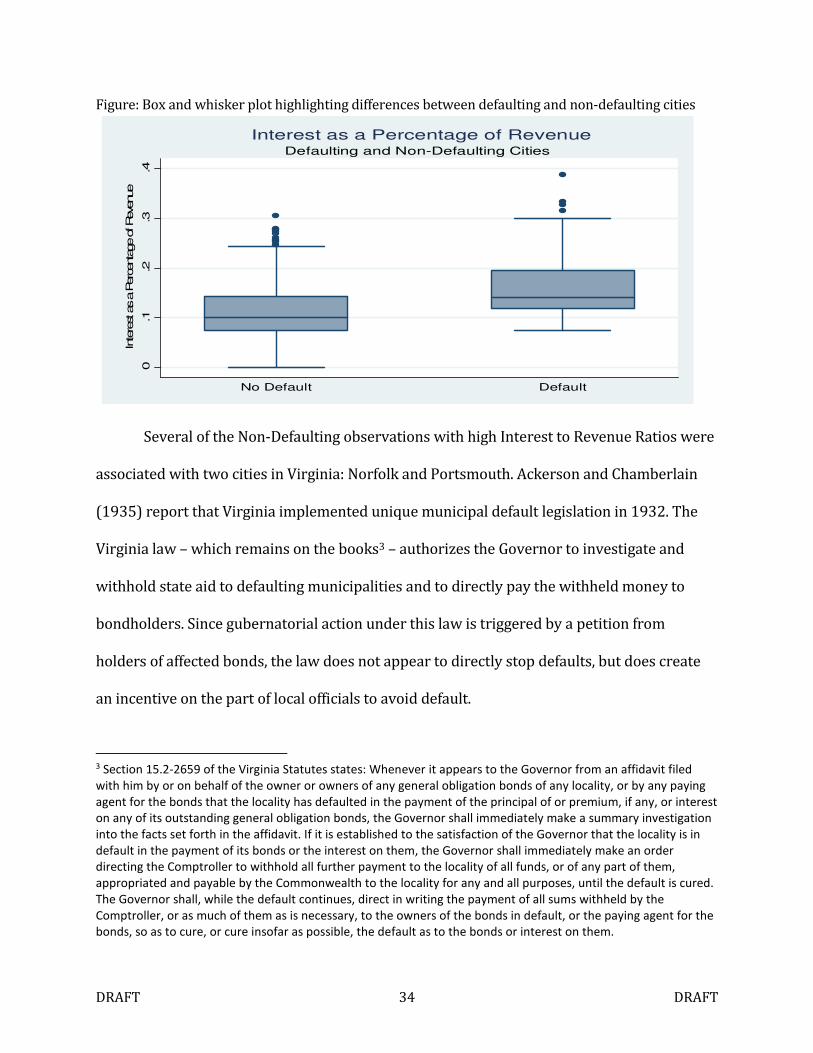
DRAFT 34 DRAFT
Figure: Box and whisker plot highlighting differences between defaulting and non-defaulting cities
Several of the Non-Defaulting observations with high Interest to Revenue Ratios were
associated with two cities in Virginia: Norfolk and Portsmouth. Ackerson and Chamberlain
(1935) report that Virginia implemented unique municipal default legislation in 1932. The
Virginia law – which remains on the books3 – authorizes the Governor to investigate and
withhold state aid to defaulting municipalities and to directly pay the withheld money to
bondholders. Since gubernatorial action under this law is triggered by a petition from
holders of affected bonds, the law does not appear to directly stop defaults, but does create
an incentive on the part of local officials to avoid default.
3 Section 15.2-2659 of the Virginia Statutes states: Whenever it appears to the Governor from an affidavit filed
with him by or on behalf of the owner or owners of any general obligation bonds of any locality, or by any paying
agent for the bonds that the locality has defaulted in the payment of the principal of or premium, if any, or interest
on any of its outstanding general obligation bonds, the Governor shall immediately make a summary investigation
into the facts set forth in the affidavit. If it is established to the satisfaction of the Governor that the locality is in
default in the payment of its bonds or the interest on them, the Governor shall immediately make an order
directing the Comptroller to withhold all further payment to the locality of all funds, or of any part of them,
appropriated and payable by the Commonwealth to the locality for any and all purposes, until the default is cured.
The Governor shall, while the default continues, direct in writing the payment of all sums withheld by the
Comptroller, or as much of them as is necessary, to the owners of the bonds in default, or the paying agent for the
bonds, so as to cure, or cure insofar as possible, the default as to the bonds or interest on them.
0.1
.2.3
.4
Intere
st as a P
ercentage of Revenue
No Default Default
Defaulting and Non-Defaulting Cities
Interest as a Percentage of Revenue
DRAFT 35 DRAFT
Aside from the absolute burden of debt services, changes in available resources may
be expected to enter into the default decision. For example, if revenues are declining, officials
may face the choice of reducing public services below baseline levels or defaulting. Thus
year-on-year revenue changes should be predictive of default. This analysis is supported by
the Depression-era data. A one sided t test for defaulting and non-defaulting governments
rejects the null hypothesis that annual revenue changes for the former group are not less
than the latter at p < 0.001. The mean revenue change for defaulting observations is -2.3%
versus +0.1% for the non-defaulting cases. Unfortunately, the use of this variable entails the
loss of some observations. Revenue change is not directly observable from the Census data of
any one year; for any given annual Census; it must be calculated by comparing revenues from
the current Census to the prior one. The first Census used in the data set is that of 1930, so
1929 revenues are required to make data from that year usable. While 1929 census data is
available, it only included 250 of the 311 cities in the 1930 census, resulting in the loss of 61
observations. Of the remaining 896 observations, 117 are associated with a defaulting city.
A city’s liquid assets may be expected to act as a cushion against default. The Census
data contains several categories of cash. Given the great variance of city size in the sample
and the need to produce a time-independent model, any cash balance must be scaled. Since
cash may be used to pay interest or principal, it can be reasonably scaled by converting it to a
proportion of outstanding debt.
The t-test shows that Cash in Public Trust Funds as a Percentage of Gross Debt fails to
reject the null hypothesis that this factor does not correctly differentiate defaulting and non-
defaulting cities at p=.01 . Since data is available for all cities in 1930, the full 957
observations can be included in the test. The mean cash balance for the 832 non-default
DRAFT 36 DRAFT
observations is 0.92% of debt, while the mean for the 125 default observations is only 0.16%.
The t statistic for the Public Fund Cash to Debt Ratio was somewhat higher than two other
ratios tested - All Cash Assets as a Percentage of Gross Debt and All Assets as a Percentage of
Gross Debt - although both of these ratios are significant at the 5% level.
Theoretically, a city could sell fixed assets to remedy a shortfall, but it may not be
feasible to do so quickly enough to avert a default. Other cash balances, such as those in
pension funds, could in theory be borrowed to make debt service payments, but there may
be legal barriers to accomplishing that. While controlling for these factors may add
explanatory power to the model, doing so does not appear to be feasible in this current
analysis.
Finally, it is reasonable to argue that a cash balance three or four years prior to a
default is less relevant than the amount of cash available closer to the time of the actual
default. The data set contains 21 observations in which the data’s as of year is coincident
with the city’s default date, i.e. the fiscal data is from the year in which the city actually
defaulted. (The other 25 defaults occurred in smaller cities after 1931, when the census
stopped collecting their financial data.) The average Cash in Public Trust Funds as a
Percentage of Gross Debt for these 21 observations is only 0.06% versus 0.83% for the
remaining 936 observations.
If data for the smaller cities post-1931 could be collected, it may be possible to
implement a balanced-panel logit regression like that described by Shumway (2001). This
approach would allow the cash variable to play a stronger role in the model. In recognition of
this potentiality, the cash variable (identified as the cash to debt ratio) is included in two of
the models described in the next section, but it falls out in the final specification.
DRAFT 37 DRAFT
Population appears in a number of the models found in the literature and is also
considered by rating agencies. In theory, population should be inversely related to default on
the grounds that smaller cities are likely to be less diversified (and thus more risky) and that
they are also more likely to have operational problems that would trigger a default.
This theory does not appear to be supported by summary statistics from the 311-city
data set. The 46 cities that defaulted had an average population of approximately 321,000
while the 265 non-defaulting cities had an average population of roughly 127,000.
Population averages provide a distorted view because they overweight larger cities. At the
time (much like now), New York was the nation’s largest city by a considerable margin. The
fact that it defaulted adds substantially to the average population of defaulting cities.
One way to address this bias is to rank the cities from 1 to 311 and then compute the
average rank of defaulting and non-defaulting cities. This analysis yields an average rank of
128 for defaulting cities and 161 for non-defaulting cities - also counter to theory. Population
is excluded from the fiscal-ratio model presented in the next section, however as mentioned
above, Appendix 1 contains extensions of the model that include population and other
socioeconomic and demographic variables.
Statistical Methodology
The current study applies a binary response technique to a larger number of
geographically representative issuers than Hempel (1971, 1973) could access. Since
municipal bankruptcy is a rare event, it is preferable to use a model that differentiates
between observations in the tail – suggesting a choice of logit over probit.
As detailed above, analysis of the data set identified three fiscal variables that have
both empirical and theoretical support. These are: (1) interest to revenue ratio, (2) revenue
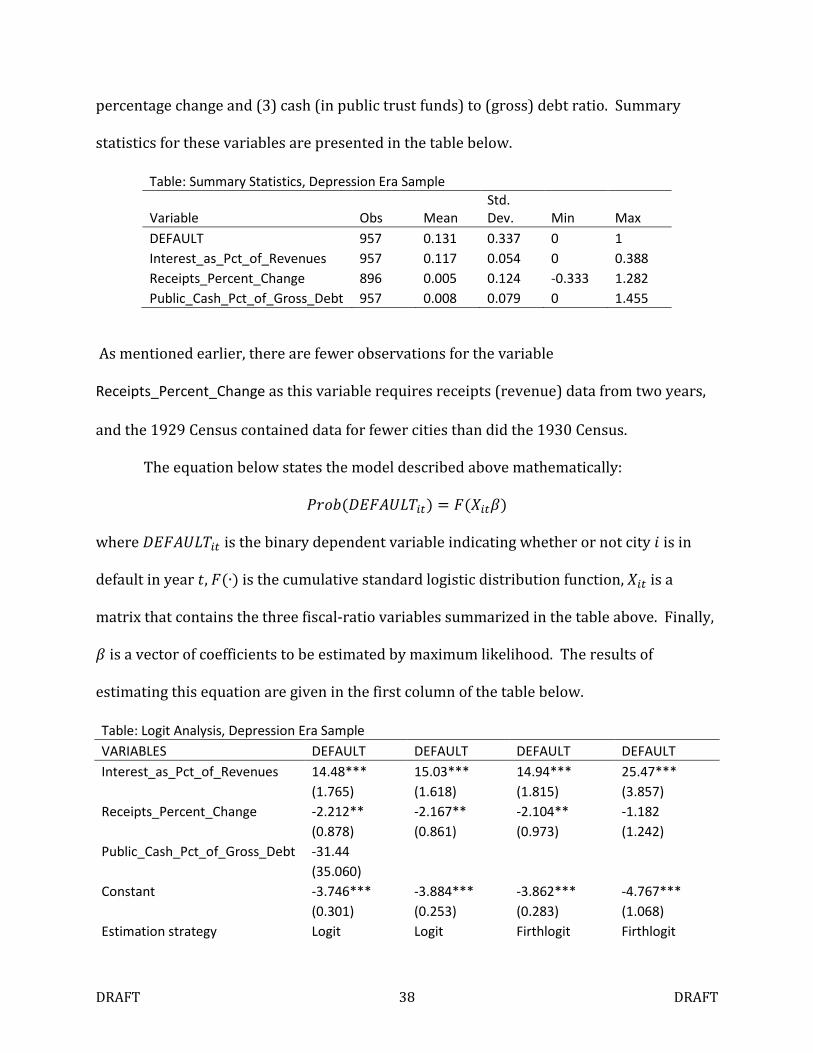
DRAFT 38 DRAFT
percentage change and (3) cash (in public trust funds) to (gross) debt ratio. Summary
statistics for these variables are presented in the table below.
Table: Summary Statistics, Depression Era Sample
Variable Obs Mean
Std.
Dev. Min Max
DEFAULT 957 0.131 0.337 0 1
Interest_as_Pct_of_Revenues 957 0.117 0.054 0 0.388
Receipts_Percent_Change 896 0.005 0.124 -0.333 1.282
Public_Cash_Pct_of_Gross_Debt 957 0.008 0.079 0 1.455
As mentioned earlier, there are fewer observations for the variable
Receipts_Percent_Change as this variable requires receipts (revenue) data from two years,
and the 1929 Census contained data for fewer cities than did the 1930 Census.
The equation below states the model described above mathematically:
����(����� �) = �(� ��)
where ����� � is the binary dependent variable indicating whether or not city � is in
default in year �, �(∙) is the cumulative standard logistic distribution function, � � is a
matrix that contains the three fiscal-ratio variables summarized in the table above. Finally,
� is a vector of coefficients to be estimated by maximum likelihood. The results of
estimating this equation are given in the first column of the table below.
Table: Logit Analysis, Depression Era Sample
VARIABLES DEFAULT DEFAULT DEFAULT DEFAULT
Interest_as_Pct_of_Revenues 14.48*** 15.03*** 14.94*** 25.47***
(1.765) (1.618) (1.815) (3.857)
Receipts_Percent_Change -2.212** -2.167** -2.104** -1.182
(0.878) (0.861) (0.973) (1.242)
Public_Cash_Pct_of_Gross_Debt -31.44
(35.060)
Constant -3.746*** -3.884*** -3.862*** -4.767***
(0.301) (0.253) (0.283) (1.068)
Estimation strategy Logit Logit Firthlogit Firthlogit
DRAFT 39 DRAFT
Standard errors in parentheses Robust Robust Homoskedastic Homoskedastic
State and year fixed effects? No No No Yes
Observations 896 896 896 896
Chi2 95.6 95.14 73.97 148.2
In the first column of the table above, one can see that the estimated coefficients on
Interest_as_Pct_of_Revenues, Receipts_Percent_Change, and Public_Cash_Pct_of_Gross_Debt
have the theoretically predicted sign; namely, high interest expense relative to revenues
increases probability of default, while a positive revenue change or high cash reserves
reduces the probability of default. However, the coefficient on
Public_Cash_Pct_of_Gross_Debt has a high standard error and the hypothesis that the true
coefficient is zero cannot be rejected at conventional confidence thresholds.
In the interest of developing a parsimonious model, the next column estimates a
restricted version of the equation; in particular in this new specification the variable
Public_Cash_Pct_of_Gross_Debt is dropped. As one can see from comparing the coefficient
estimates across the first two columns, dropping the cash variable does not substantially
change the magnitude of the other coefficients.
It is possible that a failure to include certain unobserved factors, for example state
rules that affect a city's likelihood of defaulting, are biasing the estimates. It is also possible
that the fiscal ratio variables had differential impacts on cities in different states (that is,
there may be heterogeneous effects as well as fixed effects.) While a more detailed analysis
of these possibilities is left for future research, given the panel nature of the data, it is
straightforward to implement a fixed-effect strategy as a first pass at controlling for
unobserved state and time effects (even if this does not address the possibility of
heterogeneous effects.) A complication that arises in a fixed-effect logit context, due to the
DRAFT 40 DRAFT
so-called separation problem (where a lack of variation in the dependent variable for cities
in some states prevents the possibility of estimation) requires that a new estimation
strategy must be employed if fixed effects are to be included.
The specification reported in column three includes the same variables that were
included in the specification in column two. However, the estimation strategy differs (the
coefficients in column three were estimated using Stata's firthlogit package; note, this
package does not allow for estimating robust standard errors.) Comparing the coefficient
estimates across columns two and three, one can see that the different estimation
strategies produce very similar estimates. That is, the coefficient estimates are virtually
identical, whether the estimation strategy is logit or firthlogit.
Finally, the column four presents estimates from a model with the same estimation
strategy as in column three, but which includes state and time fixed effects along with two
fiscal ratio variables. From the results in column four, one may conclude that the results in
columns two and three may understate the magnitude of the effect of the variable
Interest_as_Pct_of_Revenues while the magnitude of Receipts_Percent_Change may be
overstated.
The coefficient estimates from column two can be used to estimate the default
probabilities for cities in-sample and out-of-sample as shown below. The default probability
formula implied by the model is:
����(�����|�) =1
1 + ��(��.�����. !"∗∆%& '.(�∗)%)
Where IR = Interest_as_Pct_of_Revenues, and ∆R = Receipts_Percent_Change. Although one
may prefer to use estimates from the fixed-effect model from column four, we presented
default probability predictions using the results from column two because they are simpler
DRAFT 41 DRAFT
and aid in exposition. If one wanted to use column four’s results, the constant term should
then reflect the fixed-effect for California, which is -2.073 (so the constant would be -4.767-
2.073 = -6.84, and the coefficients on ∆R and IR would be -1.182 and 25.47 respectively.
Limitations
The use of varying numbers of observations per city (i.e. an unbalanced panel) gives
greater weight to the larger cities in estimating the model's coefficients. In addition, the
exclusion of socioeconomic variables which have been used in much of the previous
municipal credit literature is unorthodox. As already mentioned, we address these issues by
providing a set of alternative models using the Depression-era data set in the Appendix.
Further data supplementation may facilitate comparisons between city financials in
the fiscal year of default to those one, two or three years away from defaulting. It may also
permit model specifications that could incorporate a measure of the city’s cash reserves.
The explanatory variables in the foregoing analysis were based on composite
financials for all governmental units within the city. A better approach would involve using
only data from the municipal government itself – which is identified as the “city corporation”
in the Census reports.
Despite these limitations, the empirical analysis presented here supports the common
sense view that revenue declines and large debt service costs lead to defaults. The model also
allows us to quantity these vulnerabilities in a way that may permit reasonable estimation of
default probabilities for current issuers. Although the data is many decades old, it addresses
a timeless issue affecting municipal leaders in a liberal democracy: how to trade off service
demands from the electorate with the need to maintain credibility among bond investors.
DRAFT 42 DRAFT
Municipal Bond Defaults in California: History and Case Studies
Over California’s 160 year history, city bond defaults have been relatively rare.
Default activity has varied over time, peaking during the Depression. This chapter surveys
the entire history of payment defaults by California cities, with sections on each of the five
cities filing municipal bankruptcy petitions since 2001. It concludes with a brief discussion
of defaults attendant to the dissolution of Redevelopment Agencies and a review of city
fiscal emergencies.
Pre-1930
For the period from statehood through 1930, Hillhouse (1935) lists eight defaults
ascribed to California cities, but a review of original sources indicates that not all of these
are legitimate defaults in the contemporary sense.
The highest profile municipal bond default in California’s early years was that of
Placerville in 1866. Three years earlier, the city issued $100,000 in bonds to finance a rail
connection to Folsom, where service from Sacramento terminated at the time. The funds
were invested in the newly created “Placerville and Sacramento Valley Railway Company”.
The company was unable to complete the railroad, terminating it 12 miles short of the city.
Meanwhile, Placerville suffered declining population due to the end of the Gold Rush. In
1866, the city stopped making interest and principal payments. In 1873, city leaders
decided to avoid personal liability by disbanding the municipal government. In 1900, the
city government was re-established and an accommodation was made with the holders of
$34,500 still outstanding.
DRAFT 43 DRAFT
Holders of $7000 in Placerville fire department bonds issued earlier in 1863 did not
fare as well. In the case of Wichman v. City of Placerville (1905), 81 Pac. 537, the California
Supreme Court invalidated their bonds. Placerville was incorporated by the State
legislature in 1859 and then reincorporated on April 6, 1863 when it was authorized to
issue the railroad bonds. The previous city corporation issued the fire department bonds
on April 3. The court held that the bonds were obligations of a liquidated city corporation
and thus not the responsibility of the new government. California courts invalidated a
number of other city bonds listed among Hillhouse’s defaults. These cases are listed below:
City Issue Case Description
Sacramento General obligations
issued in 1854.
Bates v Gregory
(1891) 26 Pac 891
City was reincorporated in 1863. Bonds
matured in 1874 but were not
presented for payment until 1887.
Court ruled that under the statute of
limitations, the city’s liability for the
bonds lapsed in 1878.
San Diego Railroad Aid bonds
issued in 1874
McCoy v. Briant
(1878), 53 Cal 247
and Lehman v. City
of San Diego
(1897), 83 Fed 669
In McCoy v. Briant, bonds were invalid
because Board of Trustees failed to
pass a resolution authorizing them. In
Lehman v. City of San Diego, bonds
were issued after statutory
authorization was repealed but
antedated so that they would appear to
be valid.
San
Francisco
Dupont Street and
Montgomery Avenue
street construction
bonds issued in 1872
and 1877 respectively
Shapter v. San
Francisco (1901),
110 Fed. 615 and
Liebman vs. City
and County of San
Francisco (1885),
24 Fed. 705
The Dupont Street bonds were held to
be a special assessment and thus an
obligation of neighborhood property
owners rather than a general obligation
of the city. The Montgomery Avenue
bonds were determined to be
obligations of a public works
corporation, rather than city general
obligations. The public works
corporation’s taxing authority had
previously been invalidated in Mulligan
v. Smith (1881), 59 Cal 206.
Santa Cruz Water works bonds
issued in 1885
Santa Cruz Water
Company v. Kron
(1887), 15 Pac 772
Bond issued after enabling state
legislation was passed but prior to its
effective date.
Sources: Dean (1912), Court Filings
DRAFT 44 DRAFT
Hillhouse also lists a San Francisco default on Improvement Obligations, but his
reference - Sakolski (1932) - suggests that the payment failures dating to the 1850s were
not related to bonds. Apparently, San Francisco, like many gold rush era boomtowns issued
scrip to compensate vendors before taxes were collected. San Francisco was unable to
redeem the scrip with cash in a timely manner and its value depreciated. Sakolski describes
the exploits of one speculator, Peter Smith, who bought a substantial amount of the scrip at
a discount and then profited by obtaining judgments against the city – compelling it to
redeem the IOUs by selling its real estate holdings. State and local governments across the
country have resorted to issuing scrip at various times. The state of California did so in
2009 during a budget impasse. Although the use of scrip may be characterized as a default
in the popular press, it does not meet the definition of a payment default used by
contemporary bond market participants or in this study.
The last default listed by Hillhouse involved the City of Stockton in 1870. In that
year, voters overwhelmingly approved $300,000 to fund the proposed Stockton & Visalia
Railroad (Tinkham, 1923). The Council expected the new railroad to lay 15 miles of new
track terminating at the San Joacquin River and connecting it to the rest of the Central
Valley. The railroad laid one mile of new track connecting Stockton to a pre-existing
railway line, and then demanded payment from the City (Burrill, 2011). Stockton’s City
Council refused to levy taxes required to service the bonds, which appear to have been held
by the railroad. After extended litigation, the city and the railroad reached an out of court
settlement (Tinkham, 1923).
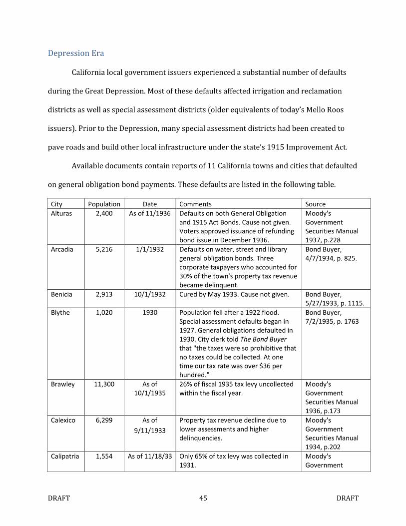
DRAFT 45 DRAFT
Depression Era
California local government issuers experienced a substantial number of defaults
during the Great Depression. Most of these defaults affected irrigation and reclamation
districts as well as special assessment districts (older equivalents of today’s Mello Roos
issuers). Prior to the Depression, many special assessment districts had been created to
pave roads and build other local infrastructure under the state’s 1915 Improvement Act.
Available documents contain reports of 11 California towns and cities that defaulted
on general obligation bond payments. These defaults are listed in the following table.
City Population Date Comments Source
Alturas 2,400 As of 11/1936 Defaults on both General Obligation
and 1915 Act Bonds. Cause not given.
Voters approved issuance of refunding
bond issue in December 1936.
Moody's
Government
Securities Manual
1937, p.228
Arcadia 5,216 1/1/1932 Defaults on water, street and library
general obligation bonds. Three
corporate taxpayers who accounted for
30% of the town's property tax revenue
became delinquent.
Bond Buyer,
4/7/1934, p. 825.
Benicia 2,913 10/1/1932 Cured by May 1933. Cause not given. Bond Buyer,
5/27/1933, p. 1115.
Blythe 1,020 1930 Population fell after a 1922 flood.
Special assessment defaults began in
1927. General obligations defaulted in
1930. City clerk told The Bond Buyer
that "the taxes were so prohibitive that
no taxes could be collected. At one
time our tax rate was over $36 per
hundred."
Bond Buyer,
7/2/1935, p. 1763
Brawley 11,300 As of
10/1/1935
26% of fiscal 1935 tax levy uncollected
within the fiscal year.
Moody's
Government
Securities Manual
1936, p.173
Calexico 6,299 As of
9/11/1933
Property tax revenue decline due to
lower assessments and higher
delinquencies.
Moody's
Government
Securities Manual
1934, p.202
Calipatria 1,554 As of 11/18/33 Only 65% of tax levy was collected in
1931.
Moody's
Government
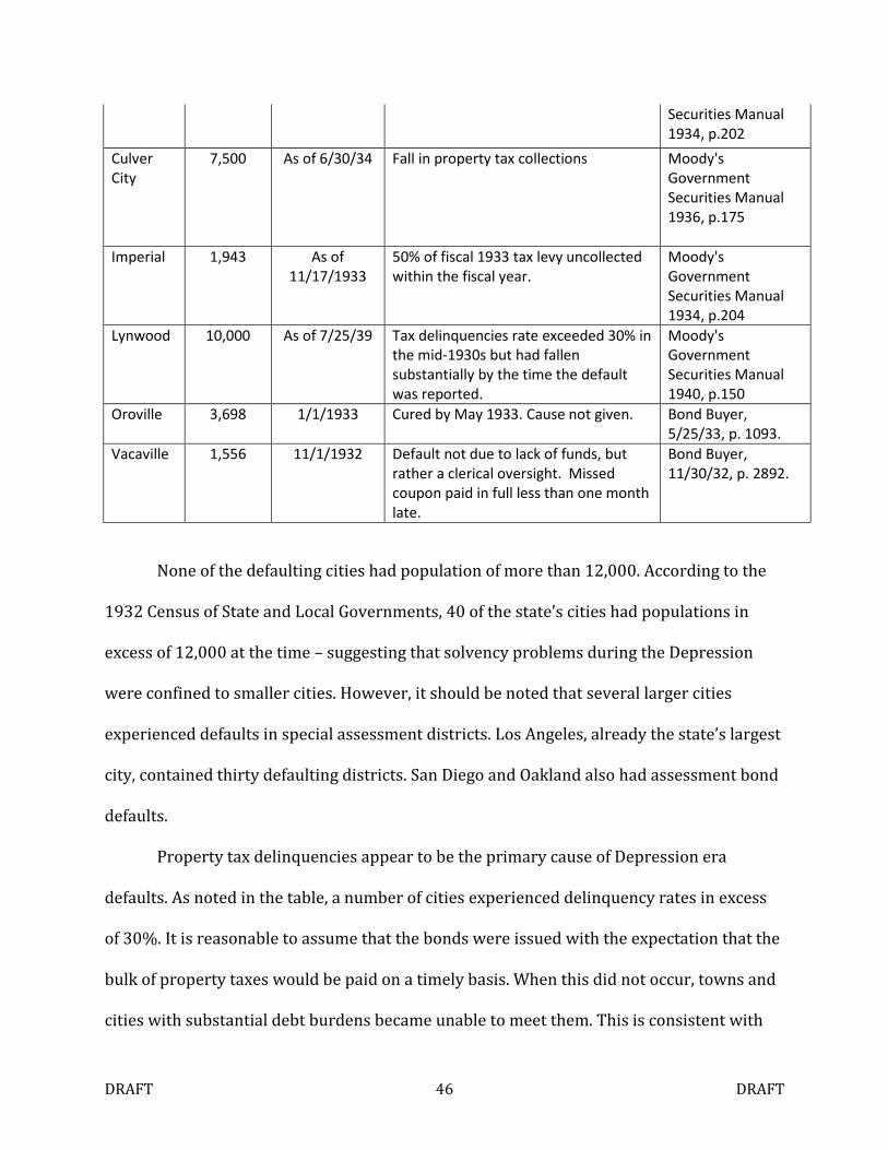
DRAFT 46 DRAFT
Securities Manual
1934, p.202
Culver
City
7,500 As of 6/30/34 Fall in property tax collections Moody's
Government
Securities Manual
1936, p.175
Imperial 1,943 As of
11/17/1933
50% of fiscal 1933 tax levy uncollected
within the fiscal year.
Moody's
Government
Securities Manual
1934, p.204
Lynwood 10,000 As of 7/25/39 Tax delinquencies rate exceeded 30% in
the mid-1930s but had fallen
substantially by the time the default
was reported.
Moody's
Government
Securities Manual
1940, p.150
Oroville 3,698 1/1/1933 Cured by May 1933. Cause not given. Bond Buyer,
5/25/33, p. 1093.
Vacaville 1,556 11/1/1932 Default not due to lack of funds, but
rather a clerical oversight. Missed
coupon paid in full less than one month
late.
Bond Buyer,
11/30/32, p. 2892.
None of the defaulting cities had population of more than 12,000. According to the
1932 Census of State and Local Governments, 40 of the state’s cities had populations in
excess of 12,000 at the time – suggesting that solvency problems during the Depression
were confined to smaller cities. However, it should be noted that several larger cities
experienced defaults in special assessment districts. Los Angeles, already the state’s largest
city, contained thirty defaulting districts. San Diego and Oakland also had assessment bond
defaults.
Property tax delinquencies appear to be the primary cause of Depression era
defaults. As noted in the table, a number of cities experienced delinquency rates in excess
of 30%. It is reasonable to assume that the bonds were issued with the expectation that the
bulk of property taxes would be paid on a timely basis. When this did not occur, towns and
cities with substantial debt burdens became unable to meet them. This is consistent with
DRAFT 47 DRAFT
the nationwide trend described in the previous chapter. It is why we include Annual
Revenue Change as a factor in our models.
Post 1940
After the Depression, benign credit conditions returned. Only three defaults by a city
(as opposed to a special assessment district) appear to have occurred between 1940 and
1993. In 1965, Redondo Beach defaulted on an unrated $9 million harbor bond issue.
According to a contemporary Moody’s Government Securities Manual (1968), the bonds
were secured by revenues from the boat harbor and taxes collected in the harbor area in
excess of the amount realized in fiscal 1958. The bonds were thus tax supported but not a
general obligation or general fund obligation of the city. According to the Wall Street
Journal (1965), “The city blamed the default on a number of factors including construction
delays, unusually severe winter storms in 1962 and the failure of expected offshore oil
revenue to materialize.” The Journal report went on to state that the 1959 feasibility study
for the harbor project had been “overly optimistic”.
In 1982, Parlier defaulted on general obligation bond payments, as well as debt
service obligations to a bank and the Farmers Home Administration. The city’s population
was reported as 2902 or 5093 by different sources perhaps because it was in the process of
annexing an unincorporated area known as West Parlier. According to the US Advisory
Commission on Intergovernmental Relations (1984), the city had $110,000 in general
obligation bonds outstanding and defaulted on a $6000 debt service payment. As of
December 15, 1982 the city had total debts of $819,089 and cash of only about $2000. A
Los Angeles Times article (Taylor, 1982a) attributed the city’s financial distress to a cost
overrun on a recently completed community center, and the initial failure of an industrial
DRAFT 48 DRAFT
park project to attract tenants. Interest in the park suffered after a carcinogen was found in
the town’s well water. The Times coverage also cited fiscal mismanagement which included
the lack of a “meaningful audit” of the city’s books between 1975 and 1982. The ACIR
report notes that the city ran persistent deficits ahead of the financial crisis, culminating in
a fiscal 1982 shortfall that amounted to 36% of revenues.
Once the extent of the crisis was determined, the city took drastic action to avoid a
municipal bankruptcy and cure its various defaults. Measures included terminating 16 of
the 22 city employees. The terminations included all of Parlier’s police officers as Fresno
County took responsibility for local law enforcement (Taylor, 1982b). By June 30, 1983 the
city had resolved all of its defaults.
In 1993, the small city of Arvin defaulted on $2.945 million of Certificates of
Participation used to finance temporary housing for farmworkers. In early 1994, it
defaulted on $7.89 million in Certificates of Participation used to finance a golf course
(Altman, 1994). Although the city considered a chapter IX filing, it appears to have reached
an accommodation with certificate owners. According to Mysak (2010), bondholders
received about 28 cents on the dollar for the defaulted golf course COPs.
In 1998, the City of Healdsburg issued $7 million in bonds on behalf of Nuestro
Hospital Group to purchase the local hospital (California Healthline, 1998). The bonds did
not constitute a claim on tax revenues and apparently went into default when the hospital
generated insufficient revenue to service them. We were unable to locate further
information about this default, which is listed in Mergent Corporation’s municipal bond
database.
DRAFT 49 DRAFT
Since 2001, five California cities have made municipal bankruptcy filings under
Chapter IX of the federal bankruptcy: Desert Hot Springs (2001), Vallejo (2008), Stockton
(2012), Mammoth Lakes (2012) and San Bernardino (2012). Four of these situations also
involved municipal bond defaults. We describe each of these cases in separate sections
below.
Desert Hot Springs
Although Desert Hot Springs December 19, 2001 bankruptcy filing (case number
6:01-bk-30756-DN Central District of California) followed an adverse court decision, its
financial problems were not wholly attributable to the lawsuit. In fact, the city’s 1999
default on unrated revenue anticipation notes occurred well before the bankruptcy filing.
According to financial statements attached to offering documents available on the
MSRB EMMA system, the city experienced large and growing all-fund deficits in fiscal 1995,
1996 and 1997. The city also experienced a large general fund deficit in fiscal 1997 –
amounting to 36% of revenues.
On August 27, 1997, the City issued $1,275,000 in Revenue Anticipation Notes
bearing a 4.75% interest rate and due the following year. These notes, rated F-2 by Fitch,
were apparently redeemed with proceeds from a second set of Revenue Anticipation Notes
issued on September 30, 1998. This second issue, totaling $1,415,000 was unrated and
carried an 8.25% interest rate – a clear signal of the city’s financial distress.
Selected fiscal statistics for Desert Hot Springs gathered from contemporaneous
financial statements are provided in the accompanying tables. All governmental fund
revenues fell 4% in fiscal 1997 but rose 7% and 8% in 1998 and 1999 respectively. These
robust increases were primarily attributable to intergovernmental revenue; real estate
DRAFT 50 DRAFT
assessment and property tax revenues were relatively weak during this period, despite the
strong national housing market. A later filing on EMMA (City of Desert Hot Springs, 2004)
shows that assessed valuations rose 3% in fiscal 1998 and fell 1% in fiscal 1999. Overall,
valuations remained stagnant throughout the mid and late 1990s, dropping slightly from
$490.6 million in fiscal 1994 to $487.0 million in 1999.
Interest expense accounted for 17% of all fund revenue in 1996 and 15% in 1997
and 1998. Also, in 1998, Pension Contributions became a significant budgetary factor,
following the city’s entry into the CalPERS. In 1999, the city’s interest expense fell due to
the default.
While aggregate governmental fund balances remained positive ahead of the city’s
default, Desert Hot Springs’ general fund balance fell below zero in fiscal 1996 and became
increasingly negative ahead of the 1999 default. General fund exhaustion appears to be the
key driver of the Desert Hot Springs default – a theme that repeats in the Vallejo, Stockton
and San Bernardino cases described below.
DRAFT 51 DRAFT
City of Desert Hot Springs - All Governmental Funds
Statement of Revenues, Expenditures and Changes in Fund Balances
1996 1997 1998 1999
Revenues
Taxes 3,910,047 3,778,247 3,921,255 3,461,885
Permits and fees 186,355 158,992 250,835 549,967
Intergovernmental 956,230 1,008,842 1,491,961 2,089,252
Licenses 145,208 120,710 115,212 113,607
Interest 582,585 323,448 343,186 256,268
Miscellaneous 268,671 398,663 56,404 202,337
Total Revenues 6,049,096 5,788,902 6,178,853 6,673,316
Expenditures
General government 1,743,931 1,872,688 1,775,738 2,052,264
Public safety 2,078,876 2,987,568 2,666,403 2,393,606
Public works 467,096 525,026 911,993 730,159
Parks and recreation 466,688 576,999 74,700 41,053
Capital outlay 851,832 425,726 771,725 60,478
Principal 918,297 2,523,996 416,657 22,253
Interest 1,009,056 860,125 895,990 365,347
Economic development 192,688 100,204 193,161 307,922
Prior year expenditures 603,889 207,344 165,894 652,175
Total Expenditures 8,332,353 10,079,676 7,872,261 6,625,257
Excess (Deficiency) of Revenues over Expends. (2,283,257) (4,290,774) (1,693,408) 48,059
Other Financing Sources (Uses) + Adjustments 427,784 424,579 118,580 (302,887)
Net Change in Fund Balances (1,855,473) (3,866,195) (1,574,828) (254,828)
Beginning Fund Balances 11,246,073 9,390,600 5,524,405 3,949,577
Ending Fund Balances 9,390,600 5,524,405 3,949,577 3,694,749
Pension Contributions 40,957 203,951 200,000
Annual Revenue Change -4.30% 6.74% 8.00%
(Interest + Pension) / Revenue 16.68% 15.57% 17.80% 8.47%
Source: Audited Financial Reports, FY 1996-1999.
Pension contributions for 1999 not available; estimated value entered.
Total Governmental Funds
DRAFT 52 DRAFT
City of Desert Hot Springs - General Fund
Statement of Revenues, Expenditures and Changes in Fund Balances
1996 1997 1998 1999
Revenues
Taxes 2,235,026 2,200,461 2,337,528 2,160,812
Permits and fees 168,770 141,281 169,281 512,408
Intergovernmental 582,359 606,870 598,647 740,025
Licenses 145,208 120,710 115,212 113,607
Interest 35,048 3,297 30,161 5,503
Miscellaneous 233,125 335,812 53,369 171,578
Total Revenues 3,399,536 3,408,431 3,304,198 3,703,933
Expenditures
General government 1,375,135 1,417,084 1,448,594 1,617,127
Public safety 2,075,894 2,955,166 2,263,685 1,690,046
Public works 93,952 81,959 233,801 177,311
Parks and recreation 53,277 121,020 74,700 21,867
Capital outlay - 134,974
Principal - 46,095 42,152
Interest - 3,994 122,047 38,000
Economic development -
Prior year expenditures 10,297 1,126
Total Expenditures 3,608,555 4,625,318 4,319,953 3,545,477
Excess (Deficiency) of Revenues over Expends. (209,019) (1,216,887) (1,015,755) 158,456
Other Financing Sources (Uses) + Adjustments (663,407) 417,079 1,026 105,441
Net Change in Fund Balances (872,426) (799,808) (1,014,729) 263,897
Beginning Fund Balances 214,503 (657,923) (1,457,731) (2,472,460)
Ending Fund Balances (657,923) (1,457,731) (2,472,460) (2,208,563)
Pension Contributions 40,957 203,951 200,000
Annual Revenue Change 0.26% -3.06% 12.10%
(Interest + Pension) / Revenue 0.00% 1.32% 9.87% 6.43%
Source: Audited Financial Statements, FY 1996-1999.
Pension contributions for 1999 not available; estimated value entered.
General Fund
DRAFT 53 DRAFT
In 2000, voters ratified additional property taxes and utility taxes that were
projected to raise $1.8 million in additional revenue (Deborah, 2000). The city may have
been able to cure its default and avoid bankruptcy had it not suffered a legal setback in
2001.
As reported by Gold (2001) in the Los Angeles Times, Desert Hot Springs chose to
enter Chapter 9 after losing a decisive battle in an 11 year fight with Silver Sage
Developers. The litigation began in 1990 after the City Council threw out the company’s
plan to build a mobile home park. The developer sued, claiming that the Council’s decision
violated the Fair Housing Act by discriminating against low income families. The initial jury
award to Silver Sage of $3 million was later reduced to $1 by a second jury. But, in July
2001, the 9th Circuit Court of Appeals reinstated the $3 million award and added another $3
million for interest and legal fees. On December 18, a federal judge declined to block Silver
Sage from seizing city assets to satisfy the judgment. Desert Hot Springs filed for Chapter IX
bankruptcy to forestall the asset seizure.
Gold’s 2001 article also notes that developers had been hesitant to start projects in
Desert Hot Springs because of the legal uncertainty. This effect may explain the relatively
stagnant real estate assessments mentioned earlier.
Vallejo
On May 23, 2008, Vallejo became the largest city to file a Chapter IX bankruptcy
petition (case number 2:08-bk-26813 Eastern District of California) since Congress first
allowed municipal bankruptcies in 1934. Vallejo’s bankruptcy involved a default on
Certificates of Participation (COPs). These certificates, unlike General Obligations or
General Fund Obligations, are not senior claims on a city’s tax revenue. Instead, they
DRAFT 54 DRAFT
represent the investor’s share in lease revenues the city agrees to pay on certain facilities.
As noted in the COPs offering materials, “the City could choose to fund other services
before making Lease Payments” and that holders have limited recourse in the event of a
default or bankruptcy (Wulf, Hansen and Company, 2003).
According to documents filed with the court and posted on the city’s web site,
bankruptcy was necessitated by the fact that the city’s general fund had been exhausted
and was expected to continue running large deficits in FY 2009. Media coverage in early
2008 also attributed the situation to high police and fire employee costs as well as
unwillingness on the part of public safety unions to make concessions (see, for example,
Jones, 2008 and Rohrs, 2008).
Data retrieved from CAFRs and other reports during this period confirm the
exhaustion of the general fund, but show large positive balances in other funds. A February
28, 2008 staff memo showed $137 million in cash balances across all funds (Mayer, 2008).
Governmental Fund balances reported as of June 30, 2008 in the CAFR were $105 million.4
It would appear that the city could have avoided or postponed bankruptcy by
lending money from other governmental funds to the general fund. The city may not have
chosen this option because of a strict reading of Governmental Accounting Standards.
Mayer (2008) states that these standards “as applied by the City and examined by our
external auditors, permit short-term interfund borrowing … only to the extent that there is
a demonstrated ability to repay these loans.” Further, staff appears to have underestimated
the costs of the Chapter IX process. In a May 6, 2008 staff memo, bankruptcy costs were
4 As discussed by GASB (2006), the concept of fund balance varies across fund types, so aggregating balances
across all funds may be misleading.
DRAFT 55 DRAFT
estimated at $750,000 to $2 million (City of Vallejo, 2008). A 2011 Wall Street Journal
article put the final cost at $9 million (White, 2011).
During each year between 1999 and 2003, the city issued COPs totaling more than
$54 million. After the city filed its bankruptcy petition, Vallejo capped interest payments
below the contractual rate. As the bankruptcy progressed, the City completely suspended
interest and principal payments twice (City of Vallejo, 2011). At the end of the bankruptcy,
the COPs were replaced with new lease agreements. Creditors are still entitled to receive all
principal originally lent, but later than expected and with less interest than required by the
original COPs. The city’s remaining debt, composed mostly of revenue bonds issued by
Enterprise (i.e., business type or non-governmental) funds, was not adjusted.
The accompanying tables show Total Governmental and General Fund values for FY
2005-2009. The bankruptcy filing occurred at the end of FY 2008. Annual government-
wide revenue fell 5% in 2006, rose 4% in 2007 and fell almost 10% in 2008. While this last
observation is consistent with the idea that falling revenue is predictive of default, it would
not have been available until well after the bankruptcy filing since the CAFR in which it
appeared was published several months after the fiscal year end. Some cities, including
Vallejo, publish interim financials, so it may have been possible to estimate this value
during the fiscal year.
Interest and retirement costs as a proportion of total revenue were not especially
high. In the year of the default, the ratio peaked at 11.36%. Overall, the parameters derived
from the Depression data do not effectively predict the Vallejo default. On the other hand,
large general fund deficits and low balances seem to have been the major contributors. As

DRAFT 56 DRAFT
suggested above, city management did not take all possible measures to stave off
insolvency and appear to have been surprised by the high cost of the bankruptcy filing.
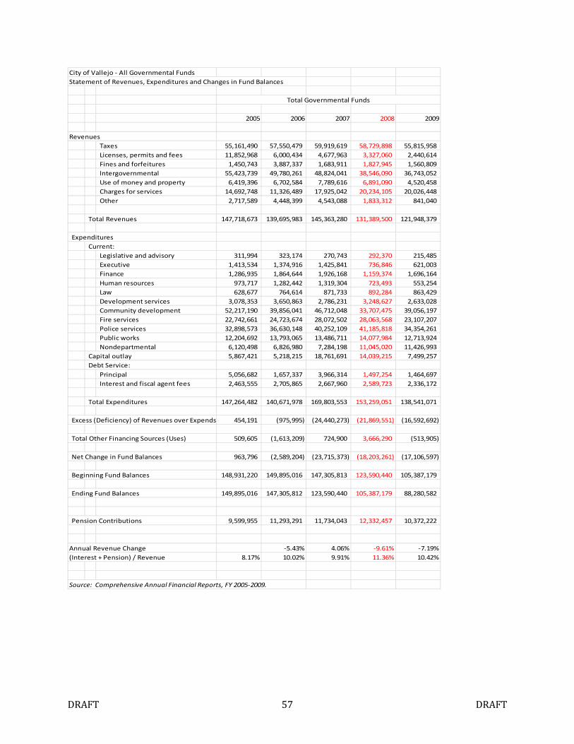
DRAFT 57 DRAFT
City of Vallejo - All Governmental Funds
Statement of Revenues, Expenditures and Changes in Fund Balances
2005 2006 2007 2008 2009
Revenues
Taxes 55,161,490 57,550,479 59,919,619 58,729,898 55,815,958
Licenses, permits and fees 11,852,968 6,000,434 4,677,963 3,327,060 2,440,614
Fines and forfeitures 1,450,743 3,887,337 1,683,911 1,827,945 1,560,809
Intergovernmental 55,423,739 49,780,261 48,824,041 38,546,090 36,743,052
Use of money and property 6,419,396 6,702,584 7,789,616 6,891,090 4,520,458
Charges for services 14,692,748 11,326,489 17,925,042 20,234,105 20,026,448
Other 2,717,589 4,448,399 4,543,088 1,833,312 841,040
Total Revenues 147,718,673 139,695,983 145,363,280 131,389,500 121,948,379
Expenditures
Current:
Legislative and advisory 311,994 323,174 270,743 292,370 215,485
Executive 1,413,534 1,374,916 1,425,841 736,846 621,003
Finance 1,286,935 1,864,644 1,926,168 1,159,374 1,696,164
Human resources 973,717 1,282,442 1,319,304 723,493 553,254
Law 628,677 764,614 871,733 892,284 863,429
Development services 3,078,353 3,650,863 2,786,231 3,248,627 2,633,028
Community development 52,217,190 39,856,041 46,712,048 33,707,475 39,056,197
Fire services 22,742,661 24,723,674 28,072,502 28,063,568 23,107,207
Police services 32,898,573 36,630,148 40,252,109 41,185,818 34,354,261
Public works 12,204,692 13,793,065 13,486,711 14,077,984 12,713,924
Nondepartmental 6,120,498 6,826,980 7,284,198 11,045,020 11,426,993
Capital outlay 5,867,421 5,218,215 18,761,691 14,039,215 7,499,257
Debt Service:
Principal 5,056,682 1,657,337 3,966,314 1,497,254 1,464,697
Interest and fiscal agent fees 2,463,555 2,705,865 2,667,960 2,589,723 2,336,172
Total Expenditures 147,264,482 140,671,978 169,803,553 153,259,051 138,541,071
Excess (Deficiency) of Revenues over Expends. 454,191 (975,995) (24,440,273) (21,869,551) (16,592,692)
Total Other Financing Sources (Uses) 509,605 (1,613,209) 724,900 3,666,290 (513,905)
Net Change in Fund Balances 963,796 (2,589,204) (23,715,373) (18,203,261) (17,106,597)
Beginning Fund Balances 148,931,220 149,895,016 147,305,813 123,590,440 105,387,179
Ending Fund Balances 149,895,016 147,305,812 123,590,440 105,387,179 88,280,582
Pension Contributions 9,599,955 11,293,291 11,734,043 12,332,457 10,372,222
Annual Revenue Change -5.43% 4.06% -9.61% -7.19%
(Interest + Pension) / Revenue 8.17% 10.02% 9.91% 11.36% 10.42%
Source: Comprehensive Annual Financial Reports, FY 2005-2009.
Total Governmental Funds
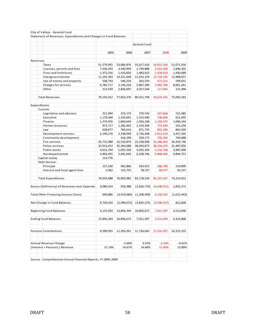
DRAFT 58 DRAFT
City of Vallejo - General Fund
Statement of Revenues, Expenditures and Changes in Fund Balances
2005 2006 2007 2008 2009
Revenues
Taxes 51,579,991 53,083,876 55,617,416 53,821,263 51,071,916
Licenses, permits and fees 7,436,293 3,440,959 2,749,888 2,431,928 1,846,301
Fines and forfeitures 1,372,316 1,410,820 1,483,923 1,428,818 1,430,689
Intergovernmental 11,191,393 14,321,658 11,553,159 12,718,335 11,908,871
Use of money and property 558,743 546,224 262,559 473,351 599,651
Charges for services 6,782,717 2,193,226 5,867,269 7,682,796 8,061,261
Other 213,559 2,826,607 3,017,544 117,944 131,494
Total Revenues 79,135,012 77,823,370 80,551,758 78,674,435 75,050,183
Expenditures
Current:
Legislative and advisory 311,994 323,174 270,743 247,668 215,485
Executive 1,170,568 1,310,691 1,312,440 736,846 621,003
Finance 1,274,935 1,864,644 1,926,168 1,159,374 1,696,164
Human resources 973,717 1,282,442 1,319,304 723,493 553,254
Law 628,677 764,614 871,733 892,284 863,429
Development services 2,199,270 2,338,949 2,726,448 2,812,419 2,457,265
Community development - 416,290 559,173 795,304 744,688
Fire services 20,715,988 22,533,874 25,238,098 25,286,403 20,424,746
Police services 32,013,022 35,264,688 38,050,873 38,204,475 31,487,056
Public works 4,615,794 5,055,339 4,052,169 4,210,768 3,987,009
Nondepartmental 5,902,455 5,041,656 6,228,746 9,868,036 9,894,757
Capital outlay 114,776 - - - -
Debt Service:
Principal 127,330 581,866 543,912 286,700 219,899
Interest and fiscal agent fees 5,962 125,755 78,727 99,577 50,157
Total Expenditures 70,054,488 76,903,982 83,178,534 85,323,347 73,214,912
Excess (Deficiency) of Revenues over Expends. 9,080,524 919,388 (2,626,776) (6,648,912) 1,835,271
Total Other Financing Sources (Uses) 649,886 (3,919,060) (1,208,499) 3,140,555 (1,022,443)
Net Change in Fund Balances 9,730,410 (2,999,672) (3,835,275) (3,508,357) 812,828
Beginning Fund Balances 4,125,934 13,856,344 10,856,672 7,021,397 3,513,040
Ending Fund Balances 13,856,344 10,856,672 7,021,397 3,513,040 4,325,868
Pension Contributions 9,599,955 11,293,291 11,734,043 12,332,457 10,372,222
Annual Revenue Change -1.66% 3.51% -2.33% -4.61%
(Interest + Pension) / Revenue 12.14% 14.67% 14.66% 15.80% 13.89%
Source: Comprehensive Annual Financial Reports, FY 2005-2009.
General Fund
DRAFT 59 DRAFT
Mammoth Lakes
The Town of Mammoth Lakes filed a Chapter IX bankruptcy petition with the
Eastern District of California Bankruptcy Court (Case Number 2:12-bk-32463) on July 3,
2012. The town, which had 8234 residents in 2010, did not default on any of its bonded
indebtedness and the bankruptcy case was dismissed on November 16, 2012.
Mammoth Lakes filed for bankruptcy after it lost a law suit to Mammoth Lakes Land
Acquisition LLC (MLLA), exhausted its appeals and failed to convince the plaintiff to reduce
the amount of the judgment. MLLA sued the town because it reneged on a 1997
development agreement in which MLLA improved the municipal airport in exchange for
the right to build a hotel/condominium project at the site. The town did not grant approval
for the hotel/condominium project because of safety concerns expressed by the Federal
Aviation Administration, but officials were aware of these concerns when they signed the
1997 agreement (Goodwin Proctor, 2011). The original judgment of $30 million awarded in
2008 increased to over $42 million by early 2012 due to attorneys’ fees and interest.
According to the Mammoth Lakes financial statements, the town had no general
obligation bonds or revenue bonds outstanding when it filed, but did have about $2.5
million in Certificates of Participation issued in 2000 and 2004. The 2000 COPs were rated
while the 2004 issue was unrated and sold privately to Citizen’s Bank. After the bankruptcy
filing, S&P downgraded the 2000 COPs issue from BB to C (Standard & Poors, 2012a).
In the city’s initial plan of adjustment, it stated its intention to continue servicing the
2000 COPs on time and in full. On the other hand, it planned to extend the term of the 2004
Citizen’s Bank COPs by three years (Town of Mammoth Lakes, 2012a).
DRAFT 60 DRAFT
Ultimately, no default occurred because the Town reached a settlement with MLLA.
Under the settlement, MLLA agreed to accept $29.5 million plus interest paid over 23 years.
The town accommodated the annual cost of the settlement through budget cuts and by
increasing its revenue forecast (Town of Mammoth Lakes, 2012b). Once the settlement was
reached, the bankruptcy case was dismissed and S&P upgraded the 2000 COPs to BB+
(Standard & Poors, 2012b).
Stockton
The City of Stockton filed a Chapter IX petition on June 28, 2012 (case number 2:12-
bk-32118) after it was unable to secure concessions from creditors during the AB 506
mediation process.5 Most of Stockton’s municipal bonds are insured by Ambac, National
Public Finance Guarantee and Assured Guarantee.
During the AB506 discussions the City stopped making debt service payments on
2004 Lease Revenue Bonds. These bonds are secured by parking garage revenues and are
not a general obligation of the City. The bond insurer, National Public Finance Guarantee,
initially received payments from a reserve fund administered by the bond trustee. Once
that fund was exhausted the trustee took possession of the three parking facilities covered
by the lease agreement and diverted a portion of the proceeds to debt service (Wells Fargo,
2013).
In February 2013, the City reached an agreement with Ambac to scale back
payments on 2003 Certificates of Participation, but the other two insurers continued to
5 Assembly Bill 506 requires cities contemplating a bankruptcy filing to engage in a neutral evaluation process with creditors. During the neutral evaluation process, which can last up to 90 days, the city is shielded from legal action on the part of creditors.
DRAFT 61 DRAFT
press their objections to the bankruptcy filing in court. They were joined by Franklin
Templeton, which holds uninsured City obligations. On April 1, 2013, Judge Christopher
Klein upheld the City’s bankruptcy filing clearing the way for it to reduce debt service
payments without facing legal action.
Stockton’s reasons for filing a bankruptcy were given in a recent news release:
On July 1, 2012, the City had less than $2 million in cash, all of which would have been
entirely depleted within the first few days of the fiscal year. It was not even enough to
make the City’s July payroll. Thus, the City would not have been able to pay its
employees, let alone its creditors, during any month of the 2012-2013 fiscal year. ... The
City could not balance its budget outside of chapter 9, absent massive giveups by
creditors who refused to make such concessions. The proposed 2012-2013 budget that
City staff submitted to the City Council in May 2012 confirmed what the City already
knew: It could not close its $26 million “gap” and balance its budget without chapter 9
protection. Its anticipated revenues remained depressed. And while it had already made
across-the-board reductions in employee costs, the costs of healthcare, pensions, and
debt service in particular were trending upward (City of Stockton, 2013).
As of this writing, the City’s 2012 CAFR has not been filed and no data for total
governmental funds is available for the most recent fiscal year. The accompanying tables
show data for fiscal 2008-2011. General fund estimates for 2012 and 2013 were derived
from the city’s most recent budget report submitted to the City Council in March 2013. No
more recent financial statistics appear to be available on Stockton’s web site.
The 2011 data reflect $15 million in adverse prior period adjustments to the city’s
general fund balance – part of $109.7 million in such adjustments across all funds. The
adjustments are described in footnote 14 of the CAFR starting at page 129 (although the
adjustments described in the note to not appear to account for the full $109.7 million in
adjustments mentioned on page 4).
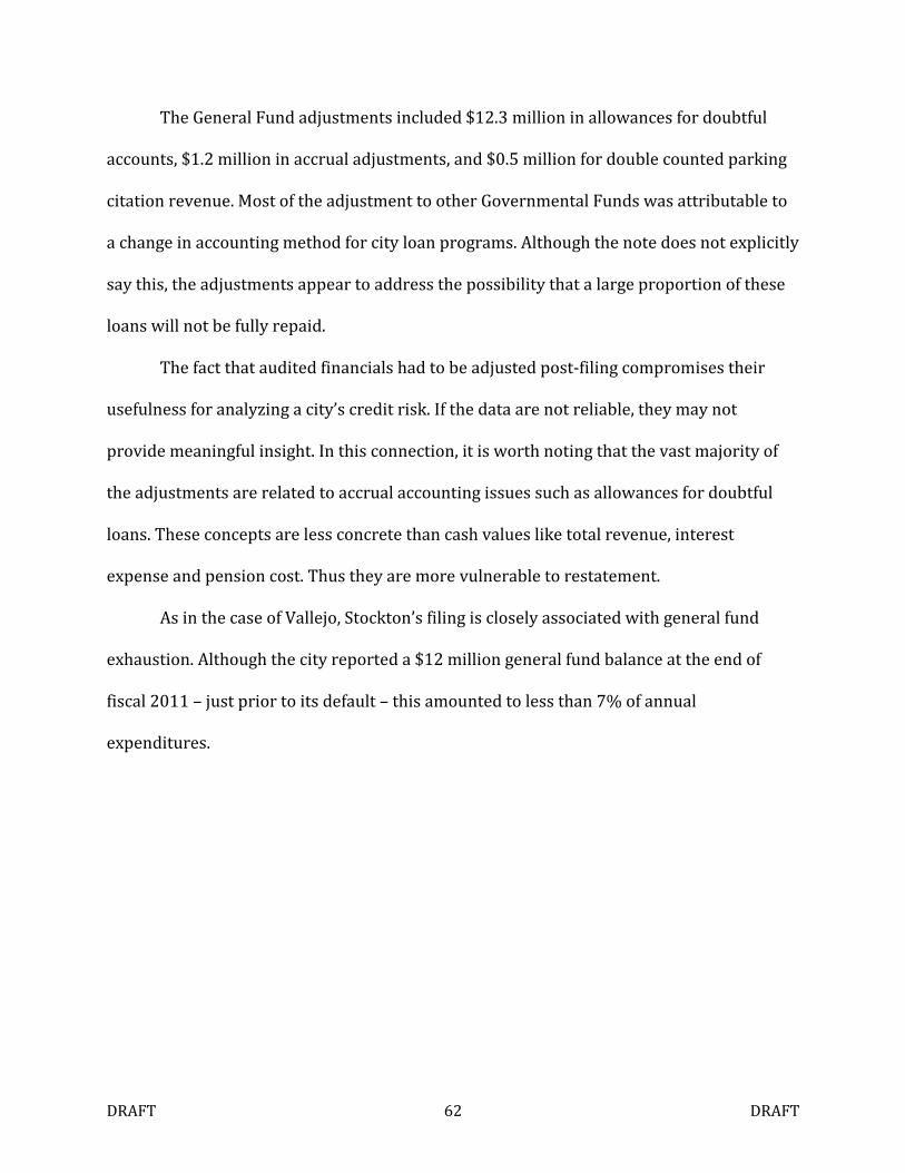
DRAFT 62 DRAFT
The General Fund adjustments included $12.3 million in allowances for doubtful
accounts, $1.2 million in accrual adjustments, and $0.5 million for double counted parking
citation revenue. Most of the adjustment to other Governmental Funds was attributable to
a change in accounting method for city loan programs. Although the note does not explicitly
say this, the adjustments appear to address the possibility that a large proportion of these
loans will not be fully repaid.
The fact that audited financials had to be adjusted post-filing compromises their
usefulness for analyzing a city’s credit risk. If the data are not reliable, they may not
provide meaningful insight. In this connection, it is worth noting that the vast majority of
the adjustments are related to accrual accounting issues such as allowances for doubtful
loans. These concepts are less concrete than cash values like total revenue, interest
expense and pension cost. Thus they are more vulnerable to restatement.
As in the case of Vallejo, Stockton’s filing is closely associated with general fund
exhaustion. Although the city reported a $12 million general fund balance at the end of
fiscal 2011 – just prior to its default – this amounted to less than 7% of annual
expenditures.
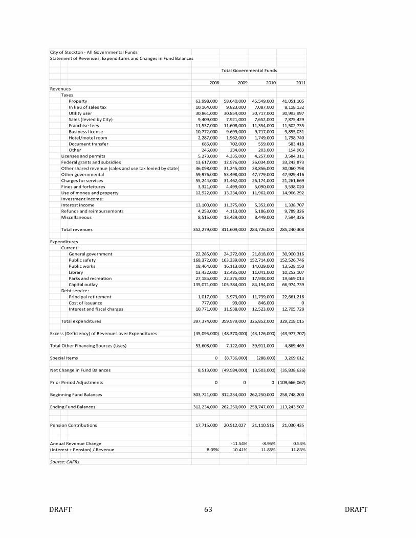
DRAFT 63 DRAFT
City of Stockton - All Governmental Funds
Statement of Revenues, Expenditures and Changes in Fund Balances
2008 2009 2010 2011
Revenues
Taxes
Property 63,998,000 58,640,000 45,549,000 41,051,105
In lieu of sales tax 10,164,000 9,823,000 7,087,000 8,118,132
Utility user 30,861,000 30,854,000 30,717,000 30,993,997
Sales (levied by City) 9,409,000 7,921,000 7,652,000 7,875,429
Franchise fees 11,537,000 11,608,000 11,354,000 11,502,735
Business license 10,772,000 9,699,000 9,717,000 9,855,031
Hotel/motel room 2,287,000 1,962,000 1,749,000 1,798,740
Document transfer 686,000 702,000 559,000 583,418
Other 246,000 234,000 203,000 154,983
Licenses and permits 5,273,000 4,335,000 4,257,000 3,584,311
Federal grants and subsidies 13,617,000 12,976,000 26,034,000 33,243,873
Other shared revenue (sales and use tax levied by state) 36,098,000 31,245,000 28,856,000 30,060,798
Other governmental 59,976,000 53,498,000 47,779,000 47,929,416
Charges for services 55,244,000 31,462,000 26,174,000 21,261,669
Fines and forfeitures 3,321,000 4,499,000 5,090,000 3,538,020
Use of money and property 12,922,000 13,234,000 11,962,000 14,966,292
Investment income:
Interest income 13,100,000 11,375,000 5,352,000 1,338,707
Refunds and reimbursements 4,253,000 4,113,000 5,186,000 9,789,326
Miscellaneous 8,515,000 13,429,000 8,449,000 7,594,326
Total revenues 352,279,000 311,609,000 283,726,000 285,240,308
Expenditures
Current:
General government 22,285,000 24,272,000 21,818,000 30,900,316
Public safety 168,372,000 163,339,000 152,714,000 152,526,746
Public works 18,464,000 16,113,000 14,029,000 13,528,150
Library 13,432,000 12,485,000 11,041,000 10,252,107
Parks and recreation 27,185,000 22,376,000 17,948,000 19,669,013
Capital outlay 135,071,000 105,384,000 84,194,000 66,974,739
Debt service:
Principal retirement 1,017,000 3,973,000 11,739,000 22,661,216
Cost of issuance 777,000 99,000 846,000 0
Interest and fiscal charges 10,771,000 11,938,000 12,523,000 12,705,728
Total expenditures 397,374,000 359,979,000 326,852,000 329,218,015
Excess (Deficiency) of Revenues over Expenditures (45,095,000) (48,370,000) (43,126,000) (43,977,707)
Total Other Financing Sources (Uses) 53,608,000 7,122,000 39,911,000 4,869,469
Special Items 0 (8,736,000) (288,000) 3,269,612
Net Change in Fund Balances 8,513,000 (49,984,000) (3,503,000) (35,838,626)
Prior Period Adjustments 0 0 0 (109,666,067)
Beginning Fund Balances 303,721,000 312,234,000 262,250,000 258,748,200
Ending Fund Balances 312,234,000 262,250,000 258,747,000 113,243,507
Pension Contributions 17,715,000 20,512,027 21,110,516 21,030,435
Annual Revenue Change -11.54% -8.95% 0.53%
(Interest + Pension) / Revenue 8.09% 10.41% 11.85% 11.83%
Source: CAFRs
Total Governmental Funds
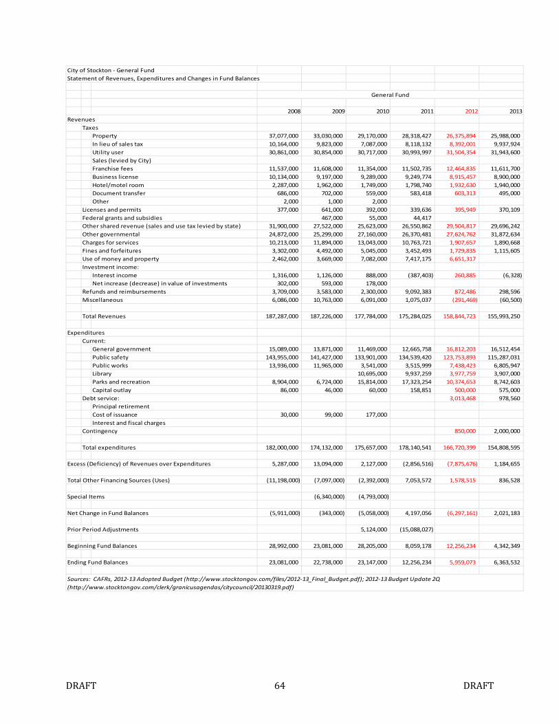
DRAFT 64 DRAFT
City of Stockton - General Fund
Statement of Revenues, Expenditures and Changes in Fund Balances
2008 2009 2010 2011 2012 2013
Revenues
Taxes
Property 37,077,000 33,030,000 29,170,000 28,318,427 26,375,894 25,988,000
In lieu of sales tax 10,164,000 9,823,000 7,087,000 8,118,132 8,392,001 9,937,924
Utility user 30,861,000 30,854,000 30,717,000 30,993,997 31,504,354 31,943,600
Sales (levied by City)
Franchise fees 11,537,000 11,608,000 11,354,000 11,502,735 12,464,835 11,611,700
Business license 10,134,000 9,197,000 9,289,000 9,249,774 8,915,457 8,900,000
Hotel/motel room 2,287,000 1,962,000 1,749,000 1,798,740 1,932,630 1,940,000
Document transfer 686,000 702,000 559,000 583,418 603,313 495,000
Other 2,000 1,000 2,000
Licenses and permits 377,000 641,000 392,000 339,636 395,949 370,109
Federal grants and subsidies 467,000 55,000 44,417
Other shared revenue (sales and use tax levied by state) 31,900,000 27,522,000 25,623,000 26,550,862 29,504,817 29,696,242
Other governmental 24,872,000 25,299,000 27,160,000 26,370,481 27,624,762 31,872,634
Charges for services 10,213,000 11,894,000 13,043,000 10,763,721 1,907,657 1,890,668
Fines and forfeitures 3,302,000 4,492,000 5,045,000 3,452,493 1,729,835 1,115,605
Use of money and property 2,462,000 3,669,000 7,082,000 7,417,175 6,651,317
Investment income:
Interest income 1,316,000 1,126,000 888,000 (387,403) 260,885 (6,328)
Net increase (decrease) in value of investments 302,000 593,000 178,000
Refunds and reimbursements 3,709,000 3,583,000 2,300,000 9,092,383 872,486 298,596
Miscellaneous 6,086,000 10,763,000 6,091,000 1,075,037 (291,469) (60,500)
Total Revenues 187,287,000 187,226,000 177,784,000 175,284,025 158,844,723 155,993,250
Expenditures
Current:
General government 15,089,000 13,871,000 11,469,000 12,665,758 16,812,203 16,512,454
Public safety 143,955,000 141,427,000 133,901,000 134,539,420 123,753,893 115,287,031
Public works 13,936,000 11,965,000 3,541,000 3,515,999 7,438,423 6,805,947
Library 10,695,000 9,937,259 3,977,759 3,907,000
Parks and recreation 8,904,000 6,724,000 15,814,000 17,323,254 10,374,653 8,742,603
Capital outlay 86,000 46,000 60,000 158,851 500,000 575,000
Debt service: 3,013,468 978,560
Principal retirement
Cost of issuance 30,000 99,000 177,000
Interest and fiscal charges
Contingency 850,000 2,000,000
Total expenditures 182,000,000 174,132,000 175,657,000 178,140,541 166,720,399 154,808,595
Excess (Deficiency) of Revenues over Expenditures 5,287,000 13,094,000 2,127,000 (2,856,516) (7,875,676) 1,184,655
Total Other Financing Sources (Uses) (11,198,000) (7,097,000) (2,392,000) 7,053,572 1,578,515 836,528
Special Items (6,340,000) (4,793,000)
Net Change in Fund Balances (5,911,000) (343,000) (5,058,000) 4,197,056 (6,297,161) 2,021,183
Prior Period Adjustments 5,124,000 (15,088,027)
Beginning Fund Balances 28,992,000 23,081,000 28,205,000 8,059,178 12,256,234 4,342,349
Ending Fund Balances 23,081,000 22,738,000 23,147,000 12,256,234 5,959,073 6,363,532
General Fund
Sources: CAFRs, 2012-13 Adopted Budget (http://www.stocktongov.com/files/2012-13_Final_Budget.pdf); 2012-13 Budget Update 2Q
(http://www.stocktongov.com/clerk/granicusagendas/citycouncil/20130319.pdf)
DRAFT 65 DRAFT
San Bernardino
The City of San Bernardino filed a Chapter IX petition on August 1, 2012 (case
number 6:12-bk-28006-MJ) after defaulting on a general fund debt service payment due
July 20, 2012.
Citing the exhaustion of the city’s general fund and an estimated fiscal year 2013
general fund deficit of $45.8 million, San Bernardino staff recommended that the city
declare bankruptcy and adopt an emergency budget that deferred debt service payments,
retiree health contributions and other items. Staff argued that these steps were necessary
to meet the City’s payroll on August 15. The affected obligations included Taxable Pension
Obligation Bonds Series 2005-A and Refunding Certificates of Participation issued in 1999.
All city obligations were insured so the defaults did not directly affect bondholders. The
affected insurers, Ambac and National Public Finance Guarantee filed objections to the
City’s bankruptcy filing.
Ultimately, the City defaulted on a July 20, 2012 pension obligation bond debt
service payment but appears to be continuing to perform on its COPs6. The City has defined
the Pension Bond as part of its overall pension expense, which it has chosen to defer.
As of this writing, the bankruptcy case is still being litigated, so the ultimate
outcome is unknown. The court docket and media reports (summarized by Shafroth, 2012-
2013) suggest that the San Bernardino case is particularly contentious for a number of
reasons (Reid, Podkul & McNeill, 2012):
6 An August 15, 2012 court filing on behalf of National said that the city had informed the insurer it would not be
making an $861,000 payment due that date. However, the EMMA system shows no payment default for the
affected bond.
DRAFT 66 DRAFT
• The City skipped the 60-day AB 506 creditor mediation process before filing, arguing that it has a right to do so because the City Council declared a fiscal emergency.
• The City suspended payments to CalPERS at the time of its filing.
• A total of 51 city employees (about 4% of the work force) retired in the three months prior to the filing, receiving $2 million for unused sick and vacation time
In October 2012, the SEC announced an informal investigation into San Bernardino’s
finances. In January 2013, both the interim city manager and finance manager resigned.
Finally, in March 2013, the State Controller’s office accused the City of improperly
transferring $529 million in former Redevelopment Agency assets to the San Bernardino
Economic Development Corporation. Given these troubles, the City is very likely to face
very large legal costs associated with the bankruptcy process. This outcome may deter
other cities from filing Chapter IX petitions.
The accompanying tables show San Bernardino’s total government and general fund
revenues and expenditures leading up to the bankruptcy filing. As of this writing, the 2012
CAFR has not appeared; incomplete data was obtained from budget documents. Since
budget documents do not use the modified accrual basis of accounting employed in CAFRs
the 2012 numbers are likely to vary somewhat from the final audited amounts that will
appear in the CAFR.
For the general fund, we provide both the original 2013 budget estimates presented
to the Council in July 2012 when it authorized the Chapter IX filing and estimates presented
in February 2013 as part of the 2013-14 budget presentation. The projected deficit shrank
from $45.8 million to $6.3 million. While most of this change is the result of the city’s
pendency plan implementation, the original deficit calculation appears to have been
pessimistic.
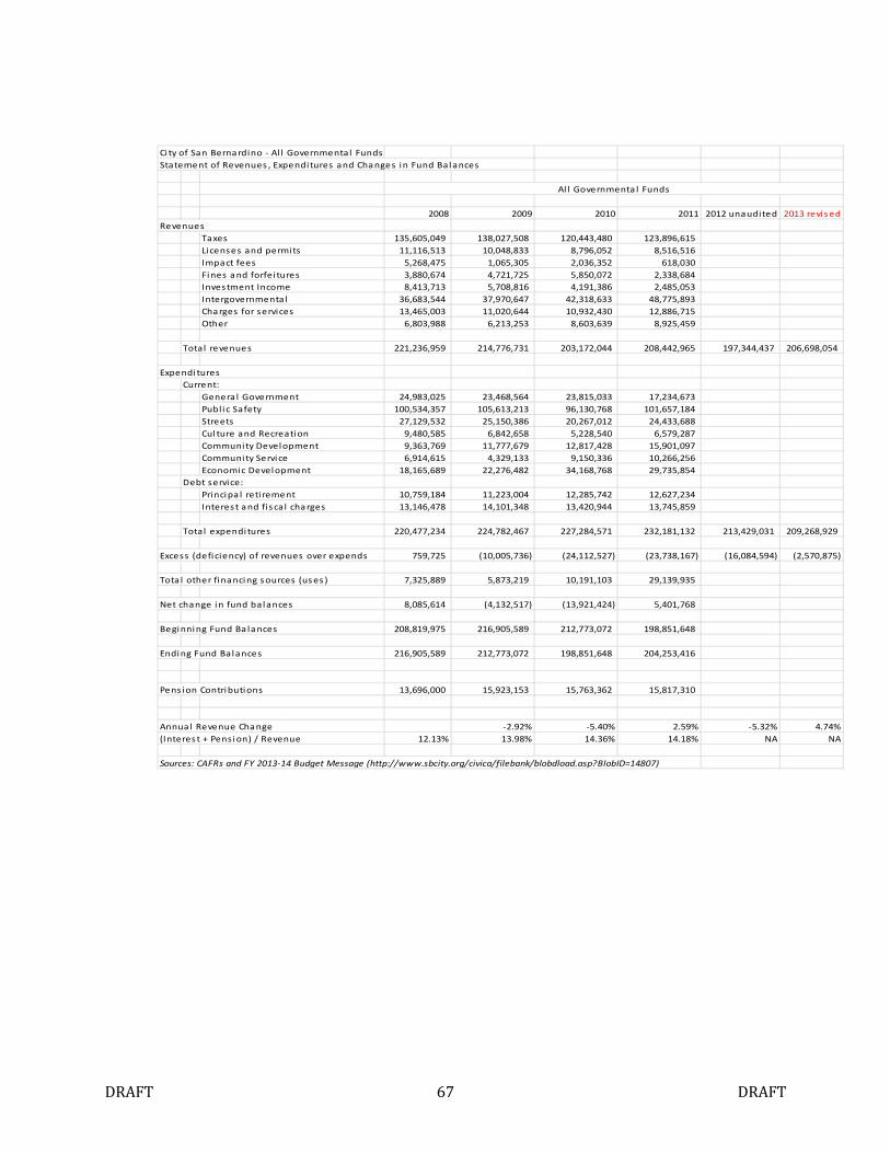
DRAFT 67 DRAFT
Ci ty of San Berna rdino - Al l Governmental Funds
Statement of Revenues , Expenditures and Cha nges in Fund Balances
2008 2009 2010 2011 2012 unaudited 2013 revi s ed
Revenues
Taxes 135,605,049 138,027,508 120,443,480 123,896,615
Licenses and permits 11,116,513 10,048,833 8,796,052 8,516,516
Impact fees 5,268,475 1,065,305 2,036,352 618,030
Fines a nd forfei tures 3,880,674 4,721,725 5,850,072 2,338,684
Inves tment Income 8,413,713 5,708,816 4,191,386 2,485,053
Intergovernmenta l 36,683,544 37,970,647 42,318,633 48,775,893
Cha rges for services 13,465,003 11,020,644 10,932,430 12,886,715
Other 6,803,988 6,213,253 8,603,639 8,925,459
Total revenues 221,236,959 214,776,731 203,172,044 208,442,965 197,344,437 206,698,054
Expendi tures
Current:
Genera l Government 24,983,025 23,468,564 23,815,033 17,234,673
Publ i c Safety 100,534,357 105,613,213 96,130,768 101,657,184
Streets 27,129,532 25,150,386 20,267,012 24,433,688
Cul ture and Recreation 9,480,585 6,842,658 5,228,540 6,579,287
Community Development 9,363,769 11,777,679 12,817,428 15,901,097
Community Service 6,914,615 4,329,133 9,150,336 10,266,256
Economic Development 18,165,689 22,276,482 34,168,768 29,735,854
Debt service:
Principa l retirement 10,759,184 11,223,004 12,285,742 12,627,234
Interes t a nd fis cal cha rges 13,146,478 14,101,348 13,420,944 13,745,859
Total expendi tures 220,477,234 224,782,467 227,284,571 232,181,132 213,429,031 209,268,929
Excess (defi ciency) of revenues over expends 759,725 (10,005,736) (24,112,527) (23,738,167) (16,084,594) (2,570,875)
Tota l other financing s ources (us es ) 7,325,889 5,873,219 10,191,103 29,139,935
Net change in fund balances 8,085,614 (4,132,517) (13,921,424) 5,401,768
Beginning Fund Ba la nces 208,819,975 216,905,589 212,773,072 198,851,648
Ending Fund Balances 216,905,589 212,773,072 198,851,648 204,253,416
Pension Contributions 13,696,000 15,923,153 15,763,362 15,817,310
Annua l Revenue Cha nge -2.92% -5.40% 2.59% -5.32% 4.74%
(Interes t + Pens ion) / Revenue 12.13% 13.98% 14.36% 14.18% NA NA
Sources: CAFRs and FY 2013-14 Budget Message (http://www.sbcity.org/civica/filebank/blobdload.asp?BlobID=14807)
Al l Governmenta l Funds
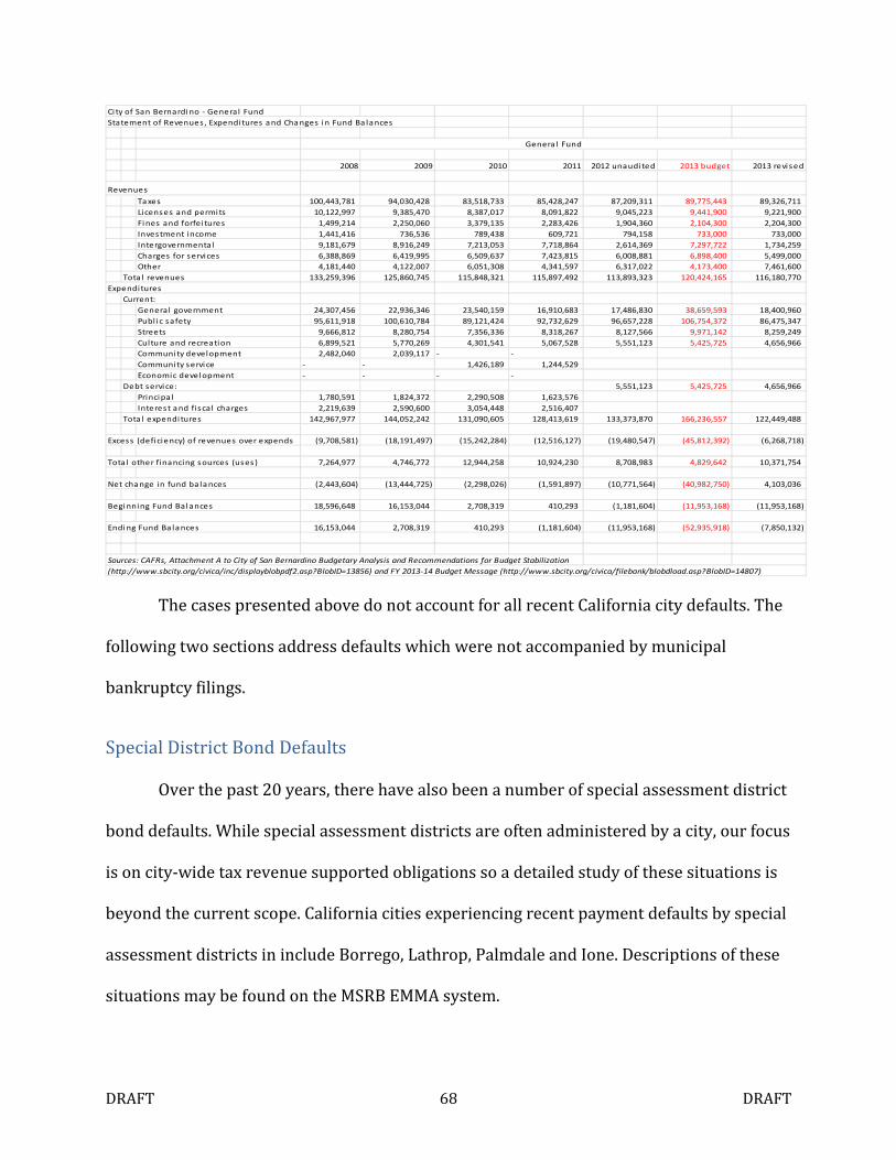
DRAFT 68 DRAFT
Ci ty of San Bernardi no - General Fund
Statement of Revenues , Expenditures a nd Cha nges i n Fund Ba la nces
2008 2009 2010 2011 2012 unaudi ted 2013 budget 2013 revi sed
Revenues
Ta xes 100,443,781 94,030,428 83,518,733 85,428,247 87,209,311 89,775,443 89,326,711
Licenses and permi ts 10,122,997 9,385,470 8,387,017 8,091,822 9,045,223 9,441,900 9,221,900
Fi nes and forfei tures 1,499,214 2,250,060 3,379,135 2,283,426 1,904,360 2,104,300 2,204,300
Investment income 1,441,416 736,536 789,438 609,721 794,158 733,000 733,000
Intergovernmental 9,181,679 8,916,249 7,213,053 7,718,864 2,614,369 7,297,722 1,734,259
Charges for services 6,388,869 6,419,995 6,509,637 7,423,815 6,008,881 6,898,400 5,499,000
Other 4,181,440 4,122,007 6,051,308 4,341,597 6,317,022 4,173,400 7,461,600
Tota l revenues 133,259,396 125,860,745 115,848,321 115,897,492 113,893,323 120,424,165 116,180,770
Expenditures
Current:
General government 24,307,456 22,936,346 23,540,159 16,910,683 17,486,830 38,659,593 18,400,960
Publ i c safety 95,611,918 100,610,784 89,121,424 92,732,629 96,657,228 106,754,372 86,475,347
Streets 9,666,812 8,280,754 7,356,336 8,318,267 8,127,566 9,971,142 8,259,249
Culture and recreation 6,899,521 5,770,269 4,301,541 5,067,528 5,551,123 5,425,725 4,656,966
Community development 2,482,040 2,039,117 - -
Community servi ce - - 1,426,189 1,244,529
Economic devel opment - - - -
Debt servi ce: 5,551,123 5,425,725 4,656,966
Princi pa l 1,780,591 1,824,372 2,290,508 1,623,576
Interest a nd fi scal charges 2,219,639 2,590,600 3,054,448 2,516,407
Tota l expendi tures 142,967,977 144,052,242 131,090,605 128,413,619 133,373,870 166,236,557 122,449,488
Excess (defi ciency) of revenues over expends (9,708,581) (18,191,497) (15,242,284) (12,516,127) (19,480,547) (45,812,392) (6,268,718)
Tota l other financing sources (uses) 7,264,977 4,746,772 12,944,258 10,924,230 8,708,983 4,829,642 10,371,754
Net cha nge in fund ba la nces (2,443,604) (13,444,725) (2,298,026) (1,591,897) (10,771,564) (40,982,750) 4,103,036
Begi nning Fund Bal ances 18,596,648 16,153,044 2,708,319 410,293 (1,181,604) (11,953,168) (11,953,168)
Endi ng Fund Ba la nces 16,153,044 2,708,319 410,293 (1,181,604) (11,953,168) (52,935,918) (7,850,132)
Sources: CAFRs, Attachment A to City of San Bernardino Budgetary Analysis and Recommendations for Budget Stabilization
(http://www.sbcity.org/civica/inc/displayblobpdf2.asp?BlobID=13856) and FY 2013-14 Budget Message (http://www.sbcity.org/civica/filebank/blobdload.asp?BlobID=14807)
Genera l Fund
The cases presented above do not account for all recent California city defaults. The
following two sections address defaults which were not accompanied by municipal
bankruptcy filings.
Special District Bond Defaults
Over the past 20 years, there have also been a number of special assessment district
bond defaults. While special assessment districts are often administered by a city, our focus
is on city-wide tax revenue supported obligations so a detailed study of these situations is
beyond the current scope. California cities experiencing recent payment defaults by special
assessment districts in include Borrego, Lathrop, Palmdale and Ione. Descriptions of these
situations may be found on the MSRB EMMA system.
DRAFT 69 DRAFT
Redevelopment Agency Defaults
In June 2011, the legislature passed and the governor signed ABX1 26, a law that
mandated dissolution of local redevelopment agencies (RDAs). The Supreme Court upheld
the law and allowed the dissolutions to take effect on February 1, 2012 (California State
Association of County Auditors, 2012). Redevelopment agency assets and liabilities mostly
reverted to the cities and counties that created them.
Many California cities took on significant amounts of bonded debt as a result of the
dissolution act, but also began to receive incremental property tax revenues necessary to
service them. While most of these transitions did not impact RDA bondholders, the cities of
Hercules and Monrovia did experience temporary defaults.
On February 1, 2012, Hercules defaulted on $2.4 million of interest payments on
RDA Tax Allocation bonds. The default did not directly impact municipal bondholders
because payment was made by Ambac, the agency’s municipal bond insurer. Ambac filed
suit against the city claiming it had failed to remit RDA related property tax collections to
the bond trustee as required. Instead the proceeds were placed in a Pooled Cash Account
(Hercules Redevelopment Agency, 2012). In March 2012, Ambac and the City settled the
litigation with the City pledging two parcels of land to the insurer (Kearney, 2012). The City
further agreed to place these two properties on the market, apparently to offset the $4.05
million property tax remittance the city had failed to make earlier (City of Hercules, 2012).
The fact that city assets had to be sold to clear the RDA default situation shows that
the Hercules episode is indicative of a fiscal insolvency. Although the City’s population is
slightly below 25,000, its fiscal indicators may be relevant to the larger cities in this study.
Unfortunately, the City had yet to publish 2011 or 2012 CAFRs at the time of this writing.
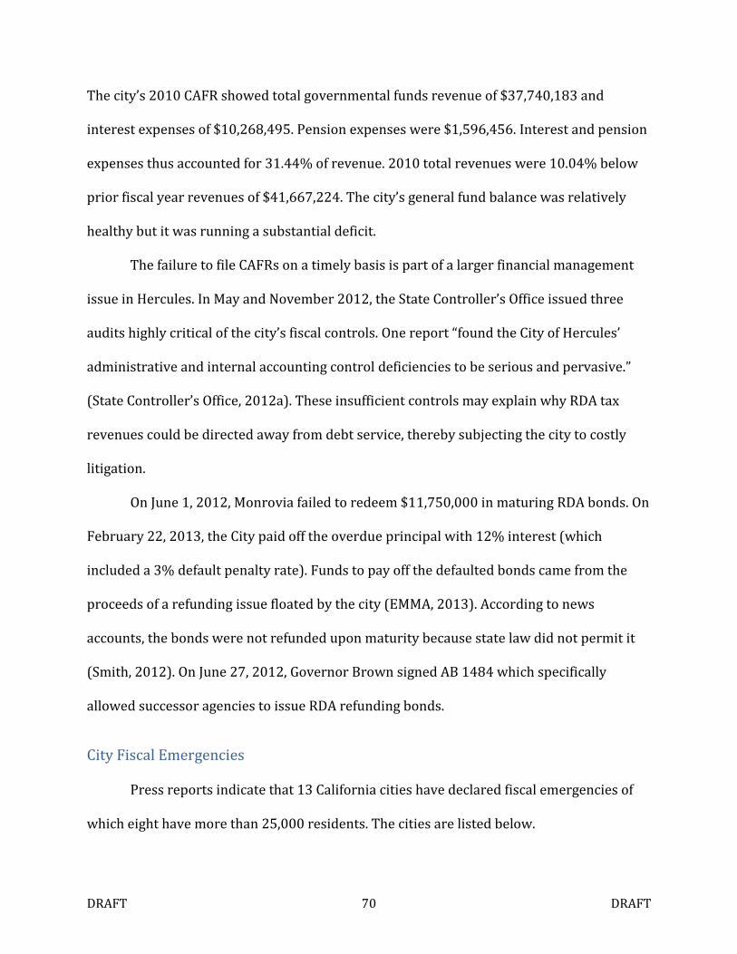
DRAFT 70 DRAFT
The city’s 2010 CAFR showed total governmental funds revenue of $37,740,183 and
interest expenses of $10,268,495. Pension expenses were $1,596,456. Interest and pension
expenses thus accounted for 31.44% of revenue. 2010 total revenues were 10.04% below
prior fiscal year revenues of $41,667,224. The city’s general fund balance was relatively
healthy but it was running a substantial deficit.
The failure to file CAFRs on a timely basis is part of a larger financial management
issue in Hercules. In May and November 2012, the State Controller’s Office issued three
audits highly critical of the city’s fiscal controls. One report “found the City of Hercules’
administrative and internal accounting control deficiencies to be serious and pervasive.”
(State Controller’s Office, 2012a). These insufficient controls may explain why RDA tax
revenues could be directed away from debt service, thereby subjecting the city to costly
litigation.
On June 1, 2012, Monrovia failed to redeem $11,750,000 in maturing RDA bonds. On
February 22, 2013, the City paid off the overdue principal with 12% interest (which
included a 3% default penalty rate). Funds to pay off the defaulted bonds came from the
proceeds of a refunding issue floated by the city (EMMA, 2013). According to news
accounts, the bonds were not refunded upon maturity because state law did not permit it
(Smith, 2012). On June 27, 2012, Governor Brown signed AB 1484 which specifically
allowed successor agencies to issue RDA refunding bonds.
City Fiscal Emergencies
Press reports indicate that 13 California cities have declared fiscal emergencies of
which eight have more than 25,000 residents. The cities are listed below.
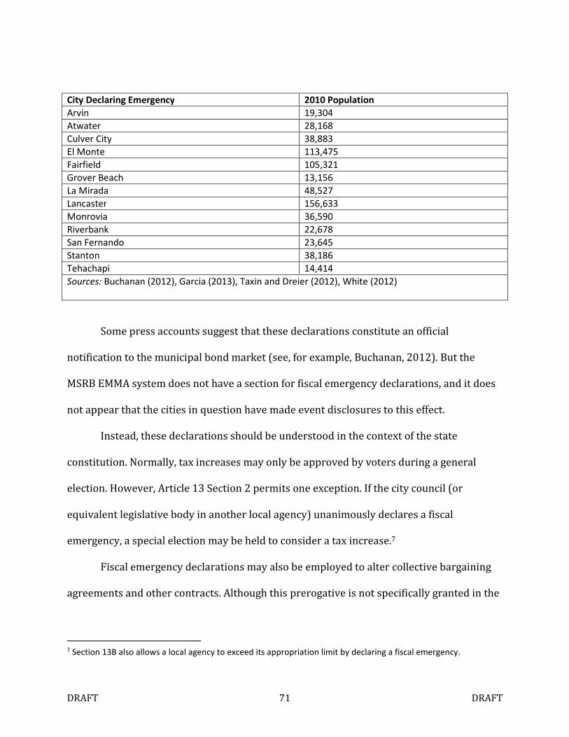
DRAFT 71 DRAFT
City Declaring Emergency 2010 Population
Arvin 19,304
Atwater 28,168
Culver City 38,883
El Monte 113,475
Fairfield 105,321
Grover Beach 13,156
La Mirada 48,527
Lancaster 156,633
Monrovia 36,590
Riverbank 22,678
San Fernando 23,645
Stanton 38,186
Tehachapi 14,414
Sources: Buchanan (2012), Garcia (2013), Taxin and Dreier (2012), White (2012)
Some press accounts suggest that these declarations constitute an official
notification to the municipal bond market (see, for example, Buchanan, 2012). But the
MSRB EMMA system does not have a section for fiscal emergency declarations, and it does
not appear that the cities in question have made event disclosures to this effect.
Instead, these declarations should be understood in the context of the state
constitution. Normally, tax increases may only be approved by voters during a general
election. However, Article 13 Section 2 permits one exception. If the city council (or
equivalent legislative body in another local agency) unanimously declares a fiscal
emergency, a special election may be held to consider a tax increase.7
Fiscal emergency declarations may also be employed to alter collective bargaining
agreements and other contracts. Although this prerogative is not specifically granted in the
7 Section 13B also allows a local agency to exceed its appropriation limit by declaring a fiscal emergency.
DRAFT 72 DRAFT
state constitution, Holtzman, Dickey & Cikes (2011) identify cases in which it has been
invoked by local agencies and supported by courts.
Consequently, fiscal emergency declarations may be seen as a way of balancing
budgets or avoiding spending reductions when a regular election is not imminent. A fiscal
emergency declaration is thus not necessarily a precursor to default or bankruptcy.
Concluding Comments
General fund exhaustion – a factor not considered in the Depression-era survey
seems to be a significant driver of recent city bankruptcies and their attendant bond
defaults. Other factors accounting for recent default activity such as adverse court
judgments and the dissolution of redevelopment agencies should be less relevant for the
purpose of modeling major city defaults. Cities below the 25,000 population threshold, like
Mammoth Lakes, are more vulnerable to lawsuit-driven defaults or bankruptcies because
their revenue base is less able to absorb multi-million dollar awards. The two RDA-related
defaults appear to be, at least in part, transitional issues.
While we have enumerated a significant number of payment difficulties in this
section, it is important to put these in context. California currently has 480 cities, and it has
had at least 200 cities through most of its history as a state. With the exception of 1933, it
appears that the municipal default rate has not exceeded 1% in any given year. In the vast
majority of years, the rate has been zero.
DRAFT 73 DRAFT
City Bond Defaults and Bankruptcies outside California
Since California’s city bond default experience is relatively limited, we supplement
the previous chapter with information regarding cities in other states. First, we consider
two high profile defaults from the 1970s and then we provide an overview of municipal
credit quality issues in other states over the last 25 years.
The 1970’s
Between the Depression and Vallejo’s 2008 bankruptcy, we are aware of only two
defaults by major US cities – both of which occurred in the 1970s. These two cases are
described in some depth in a 1984 report by the US Advisory Commission on
Intergovernmental Relations entitled Bankruptcies, Defaults and Other Local Government
Financial Emergencies. After summarizing these narratives we review these cities’ financial
statistics as reported by the US Census.
In November 1975, New York City temporarily suspended debt service payments on
short term obligations after the state legislature passed a Moratorium Act shielding the city
from bondholder lawsuits. The ACIR narrative attributes the city’s fiscal crisis to persistent
operating deficits starting in fiscal 1971. The city became increasingly dependent on short
term borrowing to fund its operations. After declaring the moratorium, New York State
took a number of actions to improve the city’s finances including the imposition of a
financial emergency control board, provision of short term loans and establishing the
Municipal Assistance Corporation to issue new bonds on behalf of the city. As a result of
these actions, the city’s budget was balanced and short term debt was replaced by longer
term obligations.
DRAFT 74 DRAFT
In December 1978, Cleveland defaulted on a $15 million bond anticipation note as
part of a larger fiscal crisis that enveloped the Ohio city. The ACIR report attributed
Cleveland’s fiscal distress to persistent operating deficits as well as poor accounting and
fiscal management practices. A June 30, 1978 audit revealed that the city had used capital
funds and other restricted funds to pay general fund obligations and that the city’s financial
records were in disarray. Cleveland’s bond ratings were then lowered and suspended,
preventing the city from rolling over its bond anticipation notes, thereby triggering the
December default. The city’s default was cured after the state auditor declared a fiscal
emergency (which allowed for the provision of state loans) and the city raised its income
tax, producing surpluses in fiscal 1980 and 1981.
The Census Bureau has been reporting city financial data since 1904. Report format,
scope and measurement definitions have changed over time, so data are not necessarily
comparable across periods. Earlier, we used Census data to obtain independent variables
for the Depression era default modeling. While two defaults are not sufficient for to create a
model, it may be useful to see how the defaulting cities ranked against peers according to
selected metrics.
During the 1970s, the Census published detailed financial statistics for cities with
population greater than about 300,000 – a class that includes New York and Cleveland. In
fiscal 1975-76, New York had the 11th highest interest-to-revenue ratio out of 48 cities in
that year’s survey. In 1978-79, Cleveland ranked 8th out of 46. While the two defaulters
were not the most indebted relative to revenue, they did place in the upper quartile of peer
cities on this measure of debt burden.

DRAFT 75 DRAFT
The Annual Revenue Change rankings were less indicative – New York was 30th and
Cleveland 21st in their respective years of default. In this case, a lower ranking (i.e., a lower
revenue change) should reflect greater risk, but in both cases, the impacted cities were
near the middle of the distribution.
The Census also reported Employee Retirement Expenditure, but the numbers do
not appear to be accurate. For example, Cleveland’s Employee Retirement Expenditure was
listed as 0 for 1978-79. Several other cities in the survey also reported zero values.
According to ACIR (1984), Cleveland did not have its own employee retirement system
during the 1970s, apparently relying on the Ohio Public Employee Retirement System
(OPERS) to manage its pension obligations. It appears that employer contributions to state
systems were excluded from the Census figures. In 1975-1976, New York’s Employee
Retirement Expenditure ranked 15th of 42 cities with non-zero values.
While General Fund balances don’t appear in the Census data, General Revenues and
General Expenditures are reported thereby allowing a calculation of General Fund
surpluses or deficits. While the Census shows New York running a surplus during the year
of its default, the city experienced substantial deficits in three of the four prior fiscal years –
consistent with the ACIR report. Cleveland had a substantial deficit in its default year and in
each of the four preceding years. In three of those years, the City’s deficits exceeded 10%
of revenue, placing it near the bottom of peer cities in the measure of general fund balance
relative to revenue.
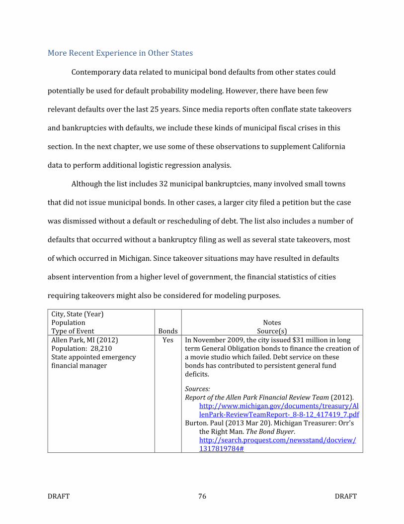
DRAFT 76 DRAFT
More Recent Experience in Other States
Contemporary data related to municipal bond defaults from other states could
potentially be used for default probability modeling. However, there have been few
relevant defaults over the last 25 years. Since media reports often conflate state takeovers
and bankruptcies with defaults, we include these kinds of municipal fiscal crises in this
section. In the next chapter, we use some of these observations to supplement California
data to perform additional logistic regression analysis.
Although the list includes 32 municipal bankruptcies, many involved small towns
that did not issue municipal bonds. In other cases, a larger city filed a petition but the case
was dismissed without a default or rescheduling of debt. The list also includes a number of
defaults that occurred without a bankruptcy filing as well as several state takeovers, most
of which occurred in Michigan. Since takeover situations may have resulted in defaults
absent intervention from a higher level of government, the financial statistics of cities
requiring takeovers might also be considered for modeling purposes.
City, State (Year) Population Type of Event Bonds
Notes Source(s)
Allen Park, MI (2012) Population: 28,210 State appointed emergency financial manager
Yes
In November 2009, the city issued $31 million in long term General Obligation bonds to finance the creation of a movie studio which failed. Debt service on these bonds has contributed to persistent general fund deficits.
Sources: Report of the Allen Park Financial Review Team (2012).
http://www.michigan.gov/documents/treasury/AllenPark-ReviewTeamReport-_8-8-12_417419_7.pdf
Burton. Paul (2013 Mar 20). Michigan Treasurer: Orr's the Right Man. The Bond Buyer. http://search.proquest.com/newsstand/docview/1317819784#
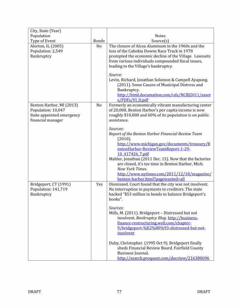
DRAFT 77 DRAFT
City, State (Year) Population Type of Event Bonds
Notes Source(s)
Alorton, IL (2005) Population: 2,549 Bankruptcy
No The closure of Alcoa Aluminum in the 1960s and the loss of the Cahokia Downs Race Track in 1978 prompted the economic decline of the Village. Lawsuits from various individuals compounded fiscal issues, leading to the Village’s bankruptcy.
Source: Levin, Richard, Jonathan Solomon & Campell Ayapong.
(2011). Some Causes of Municipal Distress and Bankruptcy. http://html.documation.com/cds/NCBJ2011/assets/PDFs/VI_D.pdf
Benton Harbor, MI (2013) Population: 10,047 State appointed emergency financial manager
No Formerly an economically vibrant manufacturing center of 20,000, Benton Harbor’s per capita income is now roughly $10,000 and 60% of its population is on public assistance.
Sources: Report of the Benton Harbor Financial Review Team
(2010). http://www.michigan.gov/documents/treasury/BentonHarbor-ReviewTeamReport-1-29-10_417426_7.pdf
Mahler, Jonathan (2011 Dec. 15). Now that the factories are closed, it’s tee time in Benton Harbor, Mich. New York Times. http://www.nytimes.com/2011/12/18/magazine/benton-harbor.html?pagewanted=all
Bridgeport, CT (1991) Population: 141,719 Bankruptcy
Yes
Dismissed. Court found that the city was not insolvent. No interruption in payments to creditors. The state backed "$53 million in bonds to balance Bridgeport's books".
Sources: Mills, M. (2011). Bridgeport – Distressed but not
insolvent. Bankruptcy Blog. http://business-finance-restructuring.weil.com/chapter-9/bridgeport-%E2%80%93-distressed-but-not-insolvent
Duby, Christopher. (1995 Oct 9). Bridgeport finally
sheds Financial Review Board. Fairfield County Business Journal. http://search.proquest.com/docview/216380696
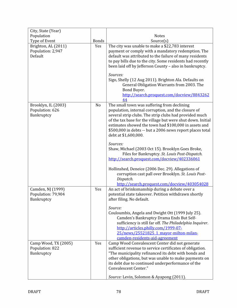
DRAFT 78 DRAFT
City, State (Year) Population Type of Event Bonds
Notes Source(s)
Brighton, AL (2011) Population: 2,947 Default
Yes The city was unable to make a $22,783 interest payment or comply with a mandatory redemption. The default was attributed to the failure of many residents to pay bills due to the city. Some residents had recently been laid off by Jefferson County – also in bankruptcy.
Sources: Sigo, Shelly (12 Aug 2011). Brighton Ala. Defaults on
General Obligation Warrants from 2003. The Bond Buyer. http://search.proquest.com/docview/884326244
Brooklyn, IL (2003) Population: 626 Bankruptcy
No The small town was suffering from declining population, internal corruption, and the closure of several strip clubs. The strip clubs had provided much of the tax base for the village but were shut down. Initial estimates showed the town had $100,000 in assets and $500,000 in debts -- but a 2006 news report places total debt at $1,600,000.
Sources: Shaw, Michael (2003 Oct 15). Brooklyn Goes Broke,
Files for Bankruptcy. St. Louis Post-Dispatch. http://search.proquest.com/docview/402336061 Hollinshed, Deneice (2006 Dec. 29). Allegations of
corruption cast pall over Brooklyn. St. Louis Post-Dispatch. http://search.proquest.com/docview/403054028
Camden, NJ (1999) Population: 79,904 Bankruptcy
Yes An act of brinksmanship during a debate over a potential state takeover. Petition withdrawn shortly after filing. No default.
Source: Couloumbis, Angela and Dwight Ott (1999 July 25).
Camden’s Bankruptcy Drama Ends But Self-sufficiency is still far off. The Philadelphia Inquirer. http://articles.philly.com/1999-07-25/news/25521825_1_mayor-milton-milan-camden-residents-aid-agreement
Camp Wood, TX (2005) Population: 822 Bankruptcy
Yes Camp Wood Convalescent Center did not generate sufficient revenue to service certificates of obligation. “The municipality refinanced its debt with bonds and other obligations, but was unable to make payments on its debt due to continued underperformance of the Convalescent Center.”
Source: Levin, Solomon & Ayapong (2011).
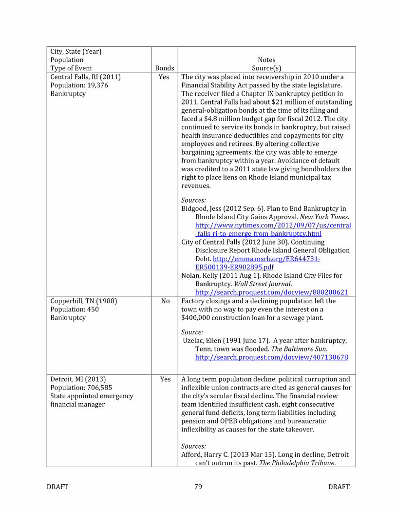
DRAFT 79 DRAFT
City, State (Year) Population Type of Event Bonds
Notes Source(s)
Central Falls, RI (2011) Population: 19,376 Bankruptcy
Yes The city was placed into receivership in 2010 under a Financial Stability Act passed by the state legislature. The receiver filed a Chapter IX bankruptcy petition in 2011. Central Falls had about $21 million of outstanding general-obligation bonds at the time of its filing and faced a $4.8 million budget gap for fiscal 2012. The city continued to service its bonds in bankruptcy, but raised health insurance deductibles and copayments for city employees and retirees. By altering collective bargaining agreements, the city was able to emerge from bankruptcy within a year. Avoidance of default was credited to a 2011 state law giving bondholders the right to place liens on Rhode Island municipal tax revenues.
Sources: Bidgood, Jess (2012 Sep. 6). Plan to End Bankruptcy in
Rhode Island City Gains Approval. New York Times. http://www.nytimes.com/2012/09/07/us/central-falls-ri-to-emerge-from-bankruptcy.html
City of Central Falls (2012 June 30). Continuing Disclosure Report Rhode Island General Obligation Debt. http://emma.msrb.org/ER644731-ER500139-ER902895.pdf
Nolan, Kelly (2011 Aug 1). Rhode Island City Files for Bankruptcy. Wall Street Journal. http://search.proquest.com/docview/880200621
Copperhill, TN (1988) Population: 450 Bankruptcy
No Factory closings and a declining population left the town with no way to pay even the interest on a $400,000 construction loan for a sewage plant.
Source: Uzelac, Ellen (1991 June 17). A year after bankruptcy,
Tenn. town was flooded. The Baltimore Sun. http://search.proquest.com/docview/407130678
Detroit, MI (2013) Population: 706,585 State appointed emergency financial manager
Yes A long term population decline, political corruption and inflexible union contracts are cited as general causes for the city’s secular fiscal decline. The financial review team identified insufficient cash, eight consecutive general fund deficits, long term liabilities including pension and OPEB obligations and bureaucratic inflexibility as causes for the state takeover.
Sources: Afford, Harry C. (2013 Mar 15). Long in decline, Detroit
can’t outrun its past. The Philadelphia Tribune.
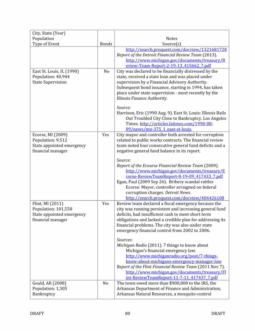
DRAFT 80 DRAFT
City, State (Year) Population Type of Event Bonds
Notes Source(s)
http://search.proquest.com/docview/1321681728 Report of the Detroit Financial Review Team (2013).
http://www.michigan.gov/documents/treasury/Review-Team-Report-2-19-13_415662_7.pdf
East St. Louis, IL (1990) Population: 40,944 State Supervision
No City was declared to be financially distressed by the state, received a state loan and was placed under supervision by a Financial Advisory Authority. Subsequent bond issuance, starting in 1994, has taken place under state supervision - most recently by the Illinois Finance Authority.
Source: Harrison, Eric (1990 Aug. 9). East St. Louis: Illinois Bails
Out Troubled City Close to Bankruptcy. Los Angeles Times. http://articles.latimes.com/1990-08-09/news/mn-375_1_east-st-louis.
Ecorse, MI (2009) Population: 9,512 State appointed emergency financial manager
Yes City mayor and controller both arrested for corruption related to public works contracts. The financial review team noted four consecutive general fund deficits and a negative general fund balance in its report.
Source: Report of the Ecourse Financial Review Team (2009).
http://www.michigan.gov/documents/treasury/Ecorse-ReviewTeamReport-8-19-09_417433_7.pdf
Egan, Paul (2009 Sep 26). Bribery scandal rattles Ecorse: Mayor, controller arraigned on federal corruption charges. Detroit News. http://search.proquest.com/docview/404426108
Flint, MI (2011) Population: 101,558 State appointed emergency financial manager
Yes Review team declared a fiscal emergency because the city was running persistent and increasing general fund deficits, had insufficient cash to meet short term obligations and lacked a credible plan for addressing its financial problems. The city was also under state emergency financial control from 2002 to 2006.
Sources: Michigan Radio (2011). 7 things to know about
Michigan’s financial emergency law. http://www.michiganradio.org/post/7-things-know-about-michigans-emergency-manager-law
Report of the Flint Financial Review Team (2011 Nov 7). http://www.michigan.gov/documents/treasury/Flint-ReviewTeamReport-11-7-11_417437_7.pdf
Gould, AR (2008) Population: 1,305 Bankruptcy
No The town owed more than $900,000 to the IRS, the Arkansas Department of Finance and Administration, Arkansas Natural Resources, a mosquito-control
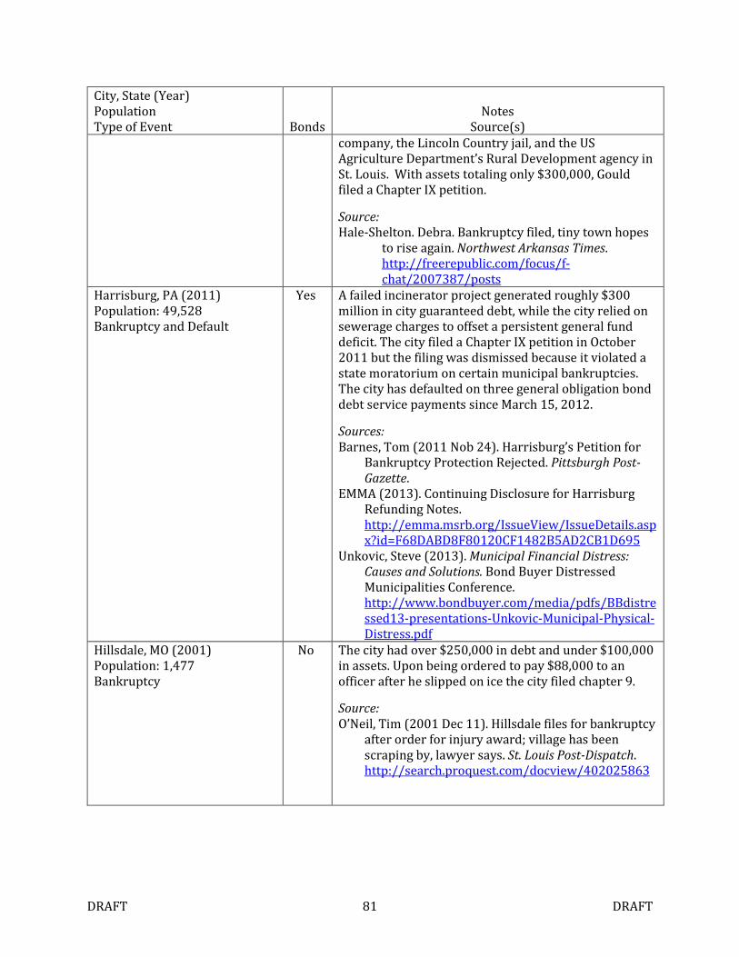
DRAFT 81 DRAFT
City, State (Year) Population Type of Event Bonds
Notes Source(s)
company, the Lincoln Country jail, and the US Agriculture Department’s Rural Development agency in St. Louis. With assets totaling only $300,000, Gould filed a Chapter IX petition.
Source: Hale-Shelton. Debra. Bankruptcy filed, tiny town hopes
to rise again. Northwest Arkansas Times. http://freerepublic.com/focus/f-chat/2007387/posts
Harrisburg, PA (2011) Population: 49,528 Bankruptcy and Default
Yes A failed incinerator project generated roughly $300 million in city guaranteed debt, while the city relied on sewerage charges to offset a persistent general fund deficit. The city filed a Chapter IX petition in October 2011 but the filing was dismissed because it violated a state moratorium on certain municipal bankruptcies. The city has defaulted on three general obligation bond debt service payments since March 15, 2012.
Sources: Barnes, Tom (2011 Nob 24). Harrisburg’s Petition for
Bankruptcy Protection Rejected. Pittsburgh Post-Gazette.
EMMA (2013). Continuing Disclosure for Harrisburg Refunding Notes. http://emma.msrb.org/IssueView/IssueDetails.aspx?id=F68DABD8F80120CF1482B5AD2CB1D695
Unkovic, Steve (2013). Municipal Financial Distress: Causes and Solutions. Bond Buyer Distressed Municipalities Conference. http://www.bondbuyer.com/media/pdfs/BBdistressed13-presentations-Unkovic-Municipal-Physical-Distress.pdf
Hillsdale, MO (2001) Population: 1,477 Bankruptcy
No The city had over $250,000 in debt and under $100,000 in assets. Upon being ordered to pay $88,000 to an officer after he slipped on ice the city filed chapter 9.
Source: O’Neil, Tim (2001 Dec 11). Hillsdale files for bankruptcy
after order for injury award; village has been scraping by, lawyer says. St. Louis Post-Dispatch. http://search.proquest.com/docview/402025863
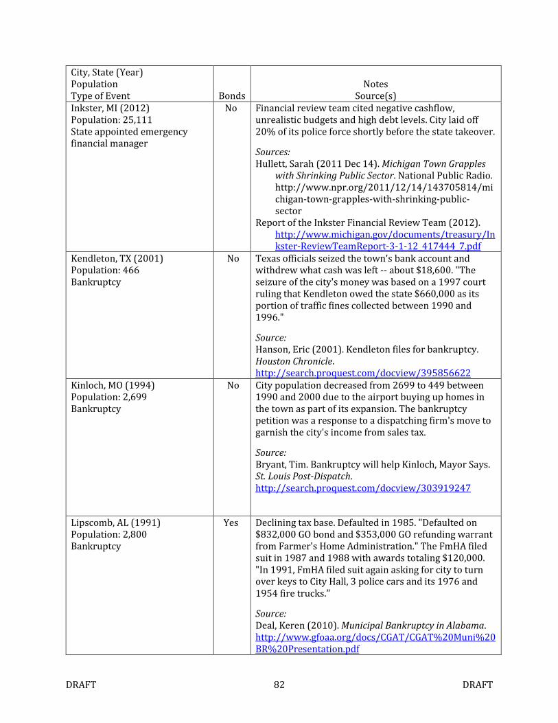
DRAFT 82 DRAFT
City, State (Year) Population Type of Event Bonds
Notes Source(s)
Inkster, MI (2012) Population: 25,111 State appointed emergency financial manager
No Financial review team cited negative cashflow, unrealistic budgets and high debt levels. City laid off 20% of its police force shortly before the state takeover.
Sources: Hullett, Sarah (2011 Dec 14). Michigan Town Grapples
with Shrinking Public Sector. National Public Radio. http://www.npr.org/2011/12/14/143705814/michigan-town-grapples-with-shrinking-public-sector
Report of the Inkster Financial Review Team (2012). http://www.michigan.gov/documents/treasury/Inkster-ReviewTeamReport-3-1-12_417444_7.pdf
Kendleton, TX (2001) Population: 466 Bankruptcy
No Texas officials seized the town's bank account and withdrew what cash was left -- about $18,600. "The seizure of the city's money was based on a 1997 court ruling that Kendleton owed the state $660,000 as its portion of traffic fines collected between 1990 and 1996."
Source: Hanson, Eric (2001). Kendleton files for bankruptcy. Houston Chronicle. http://search.proquest.com/docview/395856622
Kinloch, MO (1994) Population: 2,699 Bankruptcy
No City population decreased from 2699 to 449 between 1990 and 2000 due to the airport buying up homes in the town as part of its expansion. The bankruptcy petition was a response to a dispatching firm's move to garnish the city's income from sales tax.
Source: Bryant, Tim. Bankruptcy will help Kinloch, Mayor Says. St. Louis Post-Dispatch. http://search.proquest.com/docview/303919247
Lipscomb, AL (1991) Population: 2,800 Bankruptcy
Yes Declining tax base. Defaulted in 1985. "Defaulted on $832,000 GO bond and $353,000 GO refunding warrant from Farmer's Home Administration." The FmHA filed suit in 1987 and 1988 with awards totaling $120,000. "In 1991, FmHA filed suit again asking for city to turn over keys to City Hall, 3 police cars and its 1976 and 1954 fire trucks."
Source: Deal, Keren (2010). Municipal Bankruptcy in Alabama. http://www.gfoaa.org/docs/CGAT/CGAT%20Muni%20BR%20Presentation.pdf
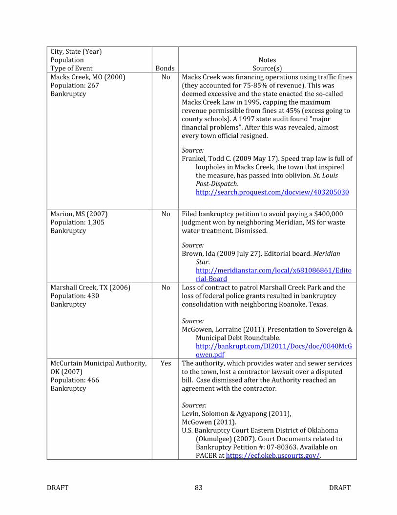
DRAFT 83 DRAFT
City, State (Year) Population Type of Event Bonds
Notes Source(s)
Macks Creek, MO (2000) Population: 267 Bankruptcy
No Macks Creek was financing operations using traffic fines (they accounted for 75-85% of revenue). This was deemed excessive and the state enacted the so-called Macks Creek Law in 1995, capping the maximum revenue permissible from fines at 45% (excess going to county schools). A 1997 state audit found "major financial problems". After this was revealed, almost every town official resigned.
Source: Frankel, Todd C. (2009 May 17). Speed trap law is full of
loopholes in Macks Creek, the town that inspired the measure, has passed into oblivion. St. Louis Post-Dispatch. http://search.proquest.com/docview/403205030
Marion, MS (2007) Population: 1,305 Bankruptcy
No Filed bankruptcy petition to avoid paying a $400,000 judgment won by neighboring Meridian, MS for waste water treatment. Dismissed.
Source: Brown, Ida (2009 July 27). Editorial board. Meridian
Star. http://meridianstar.com/local/x681086861/Editorial-Board
Marshall Creek, TX (2006) Population: 430 Bankruptcy
No Loss of contract to patrol Marshall Creek Park and the loss of federal police grants resulted in bankruptcy consolidation with neighboring Roanoke, Texas. Source: McGowen, Lorraine (2011). Presentation to Sovereign &
Municipal Debt Roundtable. http://bankrupt.com/DI2011/Docs/doc/0840McGowen.pdf
McCurtain Municipal Authority, OK (2007) Population: 466 Bankruptcy
Yes The authority, which provides water and sewer services to the town, lost a contractor lawsuit over a disputed bill. Case dismissed after the Authority reached an agreement with the contractor. Sources: Levin, Solomon & Agyapong (2011), McGowen (2011). U.S. Bankruptcy Court Eastern District of Oklahoma
(Okmulgee) (2007). Court Documents related to Bankruptcy Petition #: 07-80363. Available on PACER at https://ecf.okeb.uscourts.gov/.
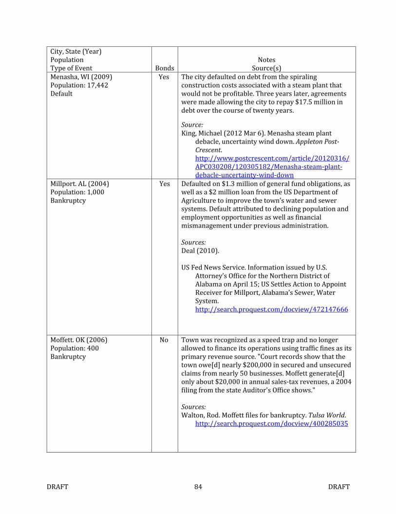
DRAFT 84 DRAFT
City, State (Year) Population Type of Event Bonds
Notes Source(s)
Menasha, WI (2009) Population: 17,442 Default
Yes The city defaulted on debt from the spiraling construction costs associated with a steam plant that would not be profitable. Three years later, agreements were made allowing the city to repay $17.5 million in debt over the course of twenty years.
Source: King, Michael (2012 Mar 6). Menasha steam plant
debacle, uncertainty wind down. Appleton Post-Crescent. http://www.postcrescent.com/article/20120316/APC030208/120305182/Menasha-steam-plant-debacle-uncertainty-wind-down
Millport. AL (2004) Population: 1,000 Bankruptcy
Yes Defaulted on $1.3 million of general fund obligations, as well as a $2 million loan from the US Department of Agriculture to improve the town’s water and sewer systems. Default attributed to declining population and employment opportunities as well as financial mismanagement under previous administration. Sources: Deal (2010). US Fed News Service. Information issued by U.S.
Attorney’s Office for the Northern District of Alabama on April 15; US Settles Action to Appoint Receiver for Millport, Alabama’s Sewer, Water System. http://search.proquest.com/docview/472147666
Moffett. OK (2006) Population: 400 Bankruptcy
No Town was recognized as a speed trap and no longer allowed to finance its operations using traffic fines as its primary revenue source. "Court records show that the town owe[d] nearly $200,000 in secured and unsecured claims from nearly 50 businesses. Moffett generate[d] only about $20,000 in annual sales-tax revenues, a 2004 filing from the state Auditor's Office shows." Sources: Walton, Rod. Moffett files for bankruptcy. Tulsa World.
http://search.proquest.com/docview/400285035
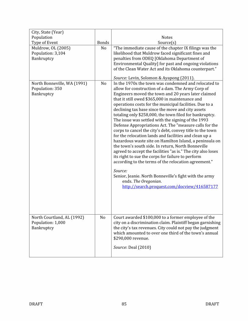
DRAFT 85 DRAFT
City, State (Year) Population Type of Event Bonds
Notes Source(s)
Muldrow, OL (2005) Population: 3,104 Bankruptcy
No “The immediate cause of the chapter IX filings was the likelihood that Muldrow faced significant fines and penalties from ODEQ [Oklahoma Department of Environmental Quality] for past and ongoing violations of the Clean Water Act and its Oklahoma counterpart.”
Source: Levin, Solomon & Ayapong (2011).
North Bonneville, WA (1991) Population: 350 Bankruptcy
No In the 1970s the town was condemned and relocated to allow for construction of a dam. The Army Corp of Engineers moved the town and 20 years later claimed that it still owed $365,000 in maintenance and operations costs for the municipal facilities. Due to a declining tax base since the move and city assets totaling only $258,000, the town filed for bankruptcy. The issue was settled with the signing of the 1993 Defense Appropriations Act. The "measure calls for the corps to cancel the city's debt, convey title to the town for the relocation lands and facilities and clean up a hazardous waste site on Hamilton Island, a peninsula on the town's south side. In return, North Bonneville agreed to accept the facilities "as is." The city also loses its right to sue the corps for failure to perform according to the terms of the relocation agreement."
Source: Senior, Jeanie. North Bonneville’s fight with the army
ends. The Oregonian. http://search.proquest.com/docview/416587177
North Courtland, AL (1992) Population: 1,000 Bankruptcy
No Court awarded $100,000 to a former employee of the city on a discrimination claim. Plaintiff began garnishing the city's tax revenues. City could not pay the judgment which amounted to over one third of the town’s annual $290,000 revenue.
Source: Deal (2010)
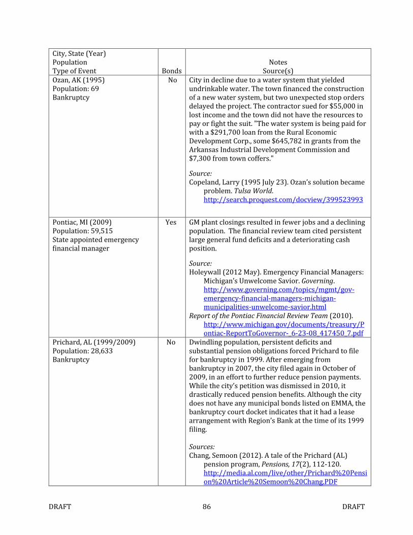
DRAFT 86 DRAFT
City, State (Year) Population Type of Event Bonds
Notes Source(s)
Ozan, AK (1995) Population: 69 Bankruptcy
No City in decline due to a water system that yielded undrinkable water. The town financed the construction of a new water system, but two unexpected stop orders delayed the project. The contractor sued for $55,000 in lost income and the town did not have the resources to pay or fight the suit. "The water system is being paid for with a $291,700 loan from the Rural Economic Development Corp., some $645,782 in grants from the Arkansas Industrial Development Commission and $7,300 from town coffers."
Source: Copeland, Larry (1995 July 23). Ozan’s solution became
problem. Tulsa World. http://search.proquest.com/docview/399523993
Pontiac, MI (2009) Population: 59,515 State appointed emergency financial manager
Yes GM plant closings resulted in fewer jobs and a declining population. The financial review team cited persistent large general fund deficits and a deteriorating cash position.
Source: Holeywall (2012 May). Emergency Financial Managers:
Michigan’s Unwelcome Savior. Governing. http://www.governing.com/topics/mgmt/gov-emergency-financial-managers-michigan-municipalities-unwelcome-savior.html
Report of the Pontiac Financial Review Team (2010). http://www.michigan.gov/documents/treasury/Pontiac-ReportToGovernor-_6-23-08_417450_7.pdf
Prichard, AL (1999/2009) Population: 28,633 Bankruptcy
No Dwindling population, persistent deficits and substantial pension obligations forced Prichard to file for bankruptcy in 1999. After emerging from bankruptcy in 2007, the city filed again in October of 2009, in an effort to further reduce pension payments. While the city’s petition was dismissed in 2010, it drastically reduced pension benefits. Although the city does not have any municipal bonds listed on EMMA, the bankruptcy court docket indicates that it had a lease arrangement with Region’s Bank at the time of its 1999 filing. Sources: Chang, Semoon (2012). A tale of the Prichard (AL)
pension program, Pensions, 17(2), 112-120. http://media.al.com/live/other/Prichard%20Pension%20Article%20Semoon%20Chang.PDF
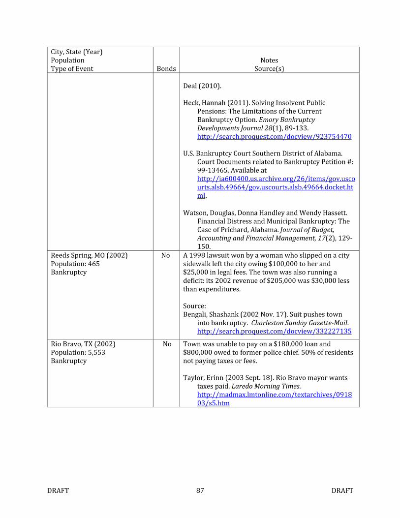
DRAFT 87 DRAFT
City, State (Year) Population Type of Event Bonds
Notes Source(s)
Deal (2010). Heck, Hannah (2011). Solving Insolvent Public
Pensions: The Limitations of the Current Bankruptcy Option. Emory Bankruptcy Developments Journal 28(1), 89-133. http://search.proquest.com/docview/923754470
U.S. Bankruptcy Court Southern District of Alabama.
Court Documents related to Bankruptcy Petition #: 99-13465. Available at http://ia600400.us.archive.org/26/items/gov.uscourts.alsb.49664/gov.uscourts.alsb.49664.docket.html.
Watson, Douglas, Donna Handley and Wendy Hassett.
Financial Distress and Municipal Bankruptcy: The Case of Prichard, Alabama. Journal of Budget, Accounting and Financial Management, 17(2), 129-150.
Reeds Spring, MO (2002) Population: 465 Bankruptcy
No A 1998 lawsuit won by a woman who slipped on a city sidewalk left the city owing $100,000 to her and $25,000 in legal fees. The town was also running a deficit: its 2002 revenue of $205,000 was $30,000 less than expenditures. Source: Bengali, Shashank (2002 Nov. 17). Suit pushes town
into bankruptcy. Charleston Sunday Gazette-Mail. http://search.proquest.com/docview/332227135
Rio Bravo, TX (2002) Population: 5,553 Bankruptcy
No Town was unable to pay on a $180,000 loan and $800,000 owed to former police chief. 50% of residents not paying taxes or fees. Taylor, Erinn (2003 Sept. 18). Rio Bravo mayor wants
taxes paid. Laredo Morning Times. http://madmax.lmtonline.com/textarchives/091803/s5.htm
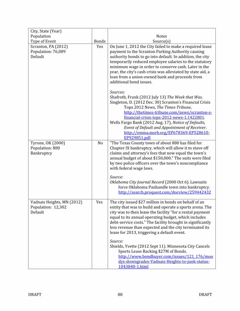
DRAFT 88 DRAFT
City, State (Year) Population Type of Event Bonds
Notes Source(s)
Scranton, PA (2012) Population: 76,089 Default
Yes On June 1, 2012 the City failed to make a required lease payment to the Scranton Parking Authority causing authority bonds to go into default. In addition, the city temporarily reduced employee salaries to the statutory minimum wage in order to conserve cash. Later in the year, the city’s cash crisis was alleviated by state aid, a loan from a union-owned bank and proceeds from additional bond issues. Sources: Shafroth, Frank (2012 July 13) The Week that Was. Singleton, D. (2012 Dec. 30) Scranton’s Financial Crisis
Tops 2012 News, The Times-Tribune, http://thetimes-tribune.com/news/scranton-s-financial-crisis-tops-2012-news-1.1422801.
Wells Fargo Bank (2012 Aug. 17), Notice of Defaults, Event of Default and Appointment of Receiver. http://emma.msrb.org/EP678369-EP528610-EP929851.pdf.
Tyrone, OK (2000) Population: 880 Bankruptcy
No "The Texas County town of about 880 has filed for Chapter IX bankruptcy, which will allow it to stave off claims and attorney’s fees that now equal the town's annual budget of about $150,000." The suits were filed by two police officers over the town's noncompliance with federal wage laws.
Source: Oklahoma City Journal Record (2000 Oct 6). Lawsuits
force Oklahoma Panhandle town into bankruptcy. http://search.proquest.com/docview/259442432
Vadnais Heights, MN (2012) Population: 12,302 Default
Yes The city issued $27 million in bonds on behalf of an entity that was to build and operate a sports arena. The city was to then lease the facility "for a rental payment equal to its annual operating budget, which includes debt-service costs." The facility brought in significantly less revenue than expected and the city terminated its lease for 2013, triggering a default event.
Source: Shields, Yvette (2012 Sept 11). Minnesota City Cancels
Sports Lease Backing $27M of Bonds. http://www.bondbuyer.com/issues/121_176/moodys-downgrades-Vadnais-Heights-to-junk-status-1043840-1.html
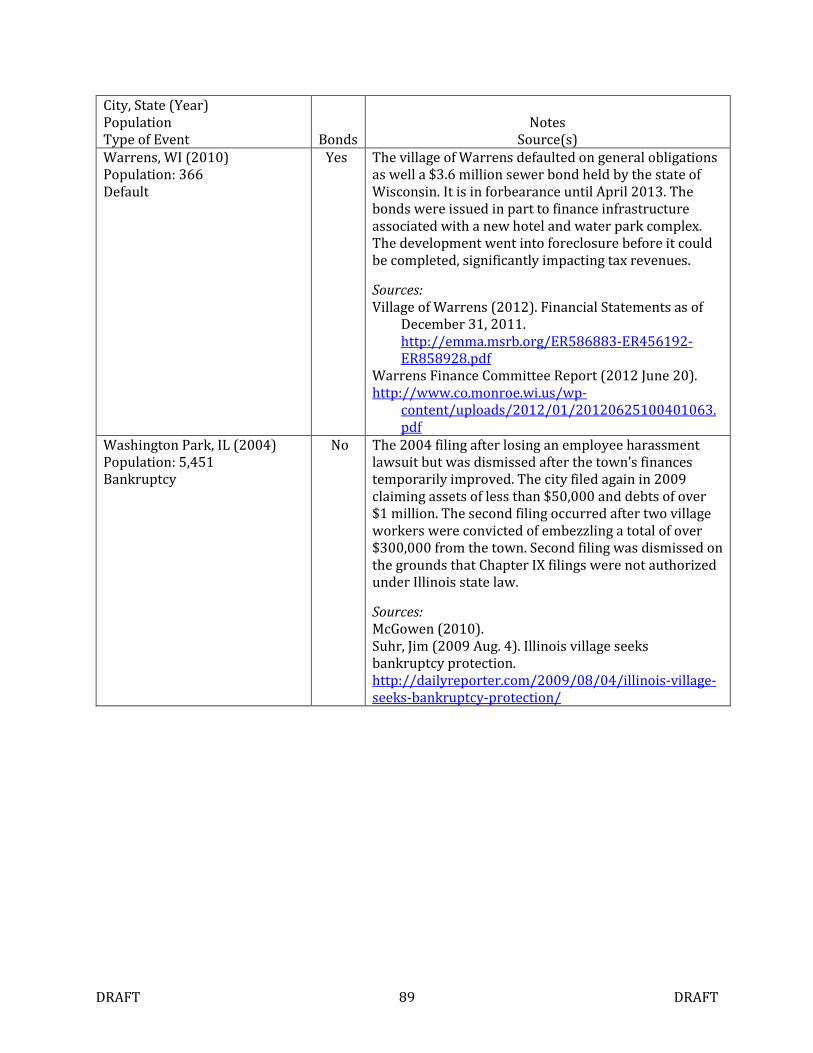
DRAFT 89 DRAFT
City, State (Year) Population Type of Event Bonds
Notes Source(s)
Warrens, WI (2010) Population: 366 Default
Yes The village of Warrens defaulted on general obligations as well a $3.6 million sewer bond held by the state of Wisconsin. It is in forbearance until April 2013. The bonds were issued in part to finance infrastructure associated with a new hotel and water park complex. The development went into foreclosure before it could be completed, significantly impacting tax revenues.
Sources: Village of Warrens (2012). Financial Statements as of
December 31, 2011. http://emma.msrb.org/ER586883-ER456192-ER858928.pdf
Warrens Finance Committee Report (2012 June 20). http://www.co.monroe.wi.us/wp-
content/uploads/2012/01/20120625100401063.pdf
Washington Park, IL (2004) Population: 5,451 Bankruptcy
No The 2004 filing after losing an employee harassment lawsuit but was dismissed after the town’s finances temporarily improved. The city filed again in 2009 claiming assets of less than $50,000 and debts of over $1 million. The second filing occurred after two village workers were convicted of embezzling a total of over $300,000 from the town. Second filing was dismissed on the grounds that Chapter IX filings were not authorized under Illinois state law.
Sources: McGowen (2010). Suhr, Jim (2009 Aug. 4). Illinois village seeks bankruptcy protection. http://dailyreporter.com/2009/08/04/illinois-village-seeks-bankruptcy-protection/
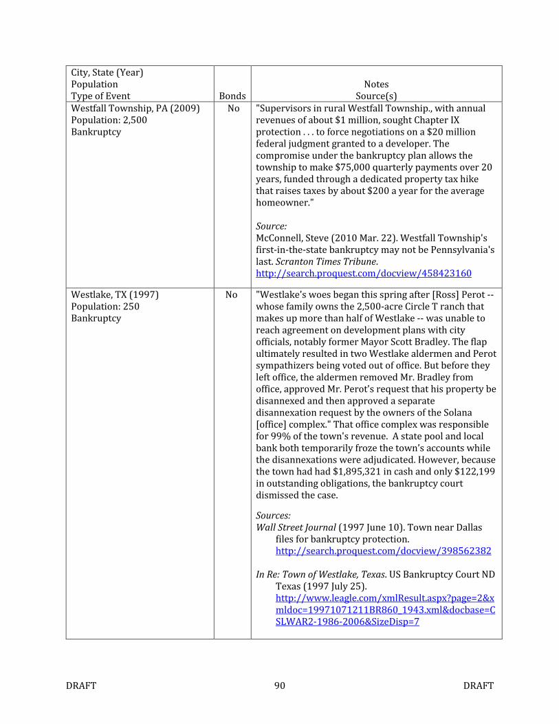
DRAFT 90 DRAFT
City, State (Year) Population Type of Event Bonds
Notes Source(s)
Westfall Township, PA (2009) Population: 2,500 Bankruptcy
No "Supervisors in rural Westfall Township., with annual revenues of about $1 million, sought Chapter IX protection . . . to force negotiations on a $20 million federal judgment granted to a developer. The compromise under the bankruptcy plan allows the township to make $75,000 quarterly payments over 20 years, funded through a dedicated property tax hike that raises taxes by about $200 a year for the average homeowner." Source: McConnell, Steve (2010 Mar. 22). Westfall Township's first-in-the-state bankruptcy may not be Pennsylvania's last. Scranton Times Tribune. http://search.proquest.com/docview/458423160
Westlake, TX (1997) Population: 250 Bankruptcy
No "Westlake's woes began this spring after [Ross] Perot -- whose family owns the 2,500-acre Circle T ranch that makes up more than half of Westlake -- was unable to reach agreement on development plans with city officials, notably former Mayor Scott Bradley. The flap ultimately resulted in two Westlake aldermen and Perot sympathizers being voted out of office. But before they left office, the aldermen removed Mr. Bradley from office, approved Mr. Perot's request that his property be disannexed and then approved a separate disannexation request by the owners of the Solana [office] complex." That office complex was responsible for 99% of the town's revenue. A state pool and local bank both temporarily froze the town’s accounts while the disannexations were adjudicated. However, because the town had had $1,895,321 in cash and only $122,199 in outstanding obligations, the bankruptcy court dismissed the case.
Sources: Wall Street Journal (1997 June 10). Town near Dallas
files for bankruptcy protection. http://search.proquest.com/docview/398562382
In Re: Town of Westlake, Texas. US Bankruptcy Court ND
Texas (1997 July 25). http://www.leagle.com/xmlResult.aspx?page=2&xmldoc=19971071211BR860_1943.xml&docbase=CSLWAR2-1986-2006&SizeDisp=7
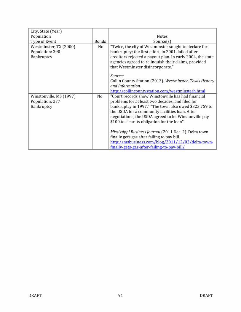
DRAFT 91 DRAFT
City, State (Year) Population Type of Event Bonds
Notes Source(s)
Westminster, TX (2000) Population: 390 Bankruptcy
No "Twice, the city of Westminster sought to declare for bankruptcy; the first effort, in 2001, failed after creditors rejected a payout plan. In early 2004, the state agencies agreed to relinquish their claims, provided that Westminster disincorporate."
Source: Collin County Station (2013). Westminster, Texas History and Information. http://collincountystation.com/westminsterh.html
Winstonville, MS (1997) Population: 277 Bankruptcy
No "Court records show Winstonville has had financial problems for at least two decades, and filed for bankruptcy in 1997." "The town also owed $323,759 to the USDA for a community facilities loan. After negotiations, the USDA agreed to let Winstonville pay $100 to clear its obligation for the loan". Mississippi Business Journal (2011 Dec. 2). Delta town finally gets gas after failing to pay bill. http://msbusiness.com/blog/2011/12/02/delta-town-finally-gets-gas-after-failing-to-pay-bill/
DRAFT 92 DRAFT
Recent Data Analysis and a Hybrid Model
The case study evidence provided in earlier suggests that general fund exhaustion
played a pivotal role in recent California defaults and bankruptcies. While interest over
revenue and annual revenue change remain intuitively attractive, they seem to have had a
lesser role in these more contemporary situations. Outside California, pension costs appear
to have played a major role in the Prichard and Central Falls bankruptcy filings.
Addressing Public Employee Pensions and OPEBs
As discussed in the Great Depression Review chapter, pensions were not seen as a
significant contributor to the spate of municipal bond defaults that occurred in the 1930s.
Since that time, California courts have repeatedly ruled that public employees and their
beneficiaries have a right to receive pension benefits according to the rules that prevailed
at the time of their employment. For example, in Kern v. City of Long Beach (29 Cal.2d 848,
1947), the California Supreme Court ruled that a fireman could not be deprived of his
pension benefits by a change to the city charter. In Betts vs. Board of Administration (21
Cal.3d 859, 1978), the Court ruled that a public agency could not apply a new benefit
formula lowering benefits to a vested employee unless it also provided a comparable,
offsetting advantage.
Pension benefits earned by existing employees thus enjoy legal protections similar
to debt service payments. Although we lack strong statistical evidence of pensions causing
municipal bond defaults, it seems appropriate to add pension expenses in the numerator of
the interest to revenue ratio. This new ratio of “uncontrollable costs” to revenues provides
DRAFT 93 DRAFT
a parsimonious way to incorporate a variable that has been the subject of extensive
political discussion.
On the other hand, we do not apply this approach to OPEB costs. As the Government
Accountability Office noted in a 2007 report, relative to pensions, “state and local law
provides much less protection for retiree health benefits. Retiree health benefits are
generally treated as an operating expense for that year’s costs on a pay-as-you-go basis and
managed together with active employee benefits.” Since OPEBs appear to be junior to debt
service and pension obligations, it seems inappropriate to include them in a ratio intended
to predict municipal bond defaults.
Since much of today’s municipal solvency discussion focuses on public employee
pension costs, it is worth taking a moment to explain how they enter into our model. We
use actual employer contributions obtained from the city’s CAFR. For California cities, this
amount is generally the same as Actuarially Required Costs (ARC) because most cities
belong to CalPERS which sets employer contribution rates based on ARC.
Since our goal is to estimate one year default probabilities, a city’s Unfunded
Actuarially Accrued Liabilities (UAAL) are less relevant. The UAAL represents the present
value of future payments needed to bring a pension system to full funding. It is not
necessary for cities to remedy pension underfunding in one year. Indeed, in the case of a
single employer system, it is not necessary for a city to remedy underfunding at all.
Pensions, like OPEBs, may be funded on as a pay-as-you-go basis, although doing so may
place an unsustainable burden on the city’s revenue base.
The model implementation we present later may be used with current balances and
annual cash flows or with projected future balances and cash flows. The latter option
DRAFT 94 DRAFT
provides forward looking default probability estimates which should be more useful to
investors. For CalPERS member cities, it is possible to obtain future employers contribution
rates from actuarial reports published on the system’s web site at
http://www.calpers.ca.gov/index.jsp?bc=/about/forms-pubs/calpers-reports/actuarial-
reports/home.xml. These reports also include a sensitivity analysis showing the effect of
different portfolio return rates on future employer contribution rates.
In April 2013, CalPERS (2013) changed its method for amortizing UAAL with the
goal of achieving full funding within 30 years. For cities and other local agency CalPERS
members, this new approach results in higher annual pension costs relative to what they
would have been under the existing actuarial method. The change will be phased in starting
in fiscal year 2016. At that time, the employer contribution rates for the median public
safety employee plan will increase from 29.3% to 30.8%. In FY 2020, the expected increase
will be from 33.9% to 39.5%. This means that, all other things being equal, an average city
will face an increase in pension costs of 5% in FY 2016 and 17% in FY 2020. In fiscal 2011,
pension costs accounted for about 7% of total governmental revenues, so the budgetary
impact of this change should average roughly 1% of revenues by FY 2020.
Statistical Analysis of Contemporary Data
We collected financial statistics for 261 California cities with population greater
than 25,000 for fiscal year 2011. Two of these cities, Stockton and San Bernardino,
defaulted the following year. Unfortunately a sample containing 2 defaults out of 261 cities
does not contain enough variation to be conducive to modeling.
We addressed this problem by making a number of additions and alterations to the
sample. Each of these changes adds default observations at the cost of compromising the
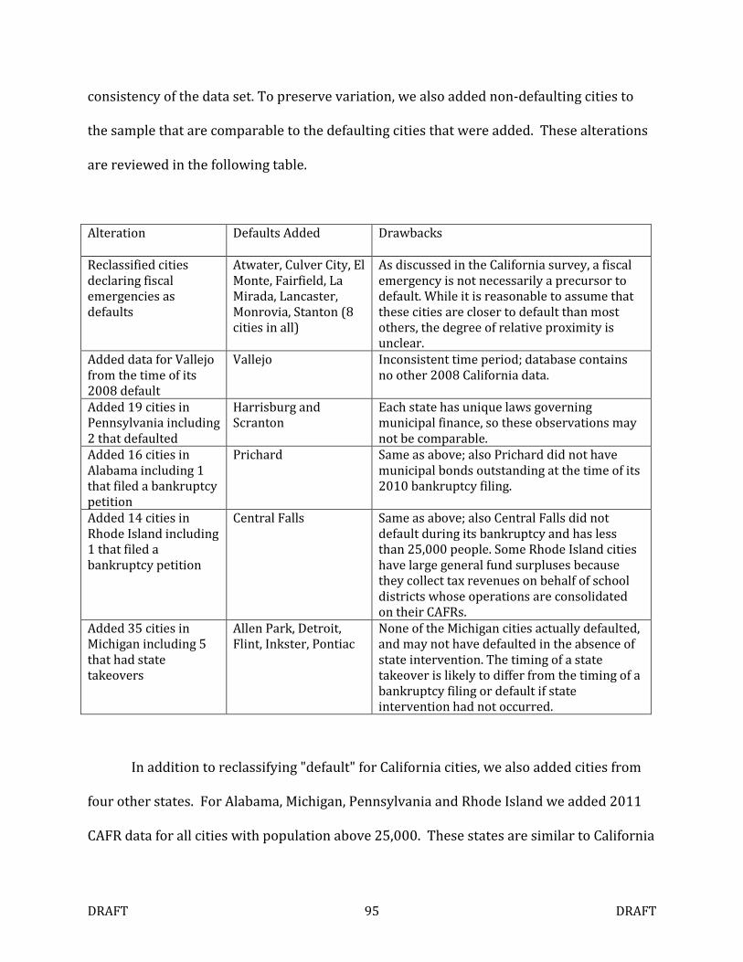
DRAFT 95 DRAFT
consistency of the data set. To preserve variation, we also added non-defaulting cities to
the sample that are comparable to the defaulting cities that were added. These alterations
are reviewed in the following table.
Alteration Defaults Added Drawbacks
Reclassified cities declaring fiscal emergencies as defaults
Atwater, Culver City, El Monte, Fairfield, La Mirada, Lancaster, Monrovia, Stanton (8 cities in all)
As discussed in the California survey, a fiscal emergency is not necessarily a precursor to default. While it is reasonable to assume that these cities are closer to default than most others, the degree of relative proximity is unclear.
Added data for Vallejo from the time of its 2008 default
Vallejo Inconsistent time period; database contains no other 2008 California data.
Added 19 cities in Pennsylvania including 2 that defaulted
Harrisburg and Scranton
Each state has unique laws governing municipal finance, so these observations may not be comparable.
Added 16 cities in Alabama including 1 that filed a bankruptcy petition
Prichard Same as above; also Prichard did not have municipal bonds outstanding at the time of its 2010 bankruptcy filing.
Added 14 cities in Rhode Island including 1 that filed a bankruptcy petition
Central Falls Same as above; also Central Falls did not default during its bankruptcy and has less than 25,000 people. Some Rhode Island cities have large general fund surpluses because they collect tax revenues on behalf of school districts whose operations are consolidated on their CAFRs.
Added 35 cities in Michigan including 5 that had state takeovers
Allen Park, Detroit, Flint, Inkster, Pontiac
None of the Michigan cities actually defaulted, and may not have defaulted in the absence of state intervention. The timing of a state takeover is likely to differ from the timing of a bankruptcy filing or default if state intervention had not occurred.
In addition to reclassifying "default" for California cities, we also added cities from
four other states. For Alabama, Michigan, Pennsylvania and Rhode Island we added 2011
CAFR data for all cities with population above 25,000. These states are similar to California
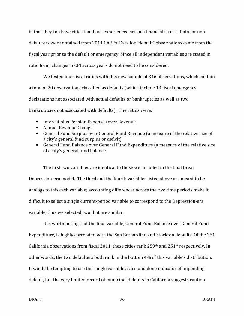
DRAFT 96 DRAFT
in that they too have cities that have experienced serious financial stress. Data for non-
defaulters were obtained from 2011 CAFRs. Data for “default” observations came from the
fiscal year prior to the default or emergency. Since all independent variables are stated in
ratio form, changes in CPI across years do not need to be considered.
We tested four fiscal ratios with this new sample of 346 observations, which contain
a total of 20 observations classified as defaults (which include 13 fiscal emergency
declarations not associated with actual defaults or bankruptcies as well as two
bankruptcies not associated with defaults). The ratios were:
• Interest plus Pension Expenses over Revenue
• Annual Revenue Change
• General Fund Surplus over General Fund Revenue (a measure of the relative size of a city’s general fund surplus or deficit)
• General Fund Balance over General Fund Expenditure (a measure of the relative size of a city’s general fund balance)
The first two variables are identical to those we included in the final Great
Depression-era model. The third and the fourth variables listed above are meant to be
analogs to this cash variable; accounting differences across the two time periods make it
difficult to select a single current-period variable to correspond to the Depression-era
variable, thus we selected two that are similar.
It is worth noting that the final variable, General Fund Balance over General Fund
Expenditure, is highly correlated with the San Bernardino and Stockton defaults. Of the 261
California observations from fiscal 2011, these cities rank 259th and 251st respectively. In
other words, the two defaulters both rank in the bottom 4% of this variable’s distribution.
It would be tempting to use this single variable as a standalone indicator of impending
default, but the very limited record of municipal defaults in California suggests caution.
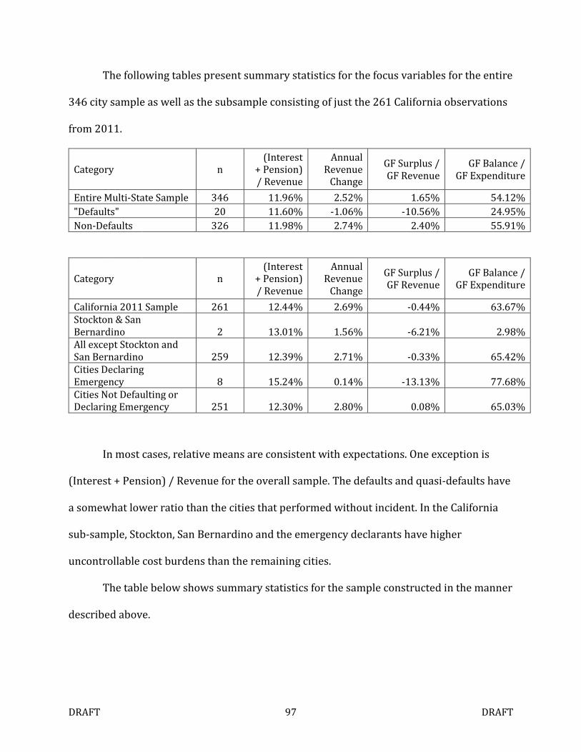
DRAFT 97 DRAFT
The following tables present summary statistics for the focus variables for the entire
346 city sample as well as the subsample consisting of just the 261 California observations
from 2011.
Category n (Interest
+ Pension) / Revenue
Annual Revenue
Change
GF Surplus / GF Revenue
GF Balance / GF Expenditure
Entire Multi-State Sample 346 11.96% 2.52% 1.65% 54.12%
"Defaults" 20 11.60% -1.06% -10.56% 24.95%
Non-Defaults 326 11.98% 2.74% 2.40% 55.91%
Category n (Interest
+ Pension) / Revenue
Annual Revenue
Change
GF Surplus / GF Revenue
GF Balance / GF Expenditure
California 2011 Sample 261 12.44% 2.69% -0.44% 63.67%
Stockton & San Bernardino 2 13.01% 1.56% -6.21% 2.98%
All except Stockton and San Bernardino 259 12.39% 2.71% -0.33% 65.42%
Cities Declaring Emergency 8 15.24% 0.14% -13.13% 77.68%
Cities Not Defaulting or Declaring Emergency 251 12.30% 2.80% 0.08% 65.03%
In most cases, relative means are consistent with expectations. One exception is
(Interest + Pension) / Revenue for the overall sample. The defaults and quasi-defaults have
a somewhat lower ratio than the cities that performed without incident. In the California
sub-sample, Stockton, San Bernardino and the emergency declarants have higher
uncontrollable cost burdens than the remaining cities.
The table below shows summary statistics for the sample constructed in the manner
described above.
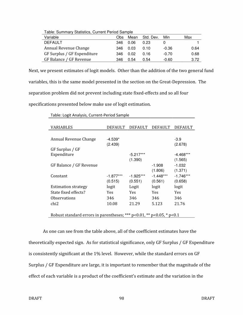
DRAFT 98 DRAFT
Table: Summary Statistics, Current Period Sample
Variable Obs Mean Std. Dev. Min Max
DEFAULT 346 0.06 0.23 0 1
Annual Revenue Change 346 0.03 0.10 -0.36 0.64
GF Surplus / GF Expenditure 346 0.02 0.16 -0.70 0.68
GF Balance / GF Revenue 346 0.54 0.54 -0.60 3.72
Next, we present estimates of logit models. Other than the addition of the two general fund
variables, this is the same model presented in the section on the Great-Depression. The
separation problem did not prevent including state fixed-effects and so all four
specifications presented below make use of logit estimation.
Table: Logit Analysis, Current-Period Sample
VARIABLES DEFAULT DEFAULT DEFAULT DEFAULT
Annual Revenue Change -4.539*
-3.9
(2.439)
(2.678)
GF Surplus / GF Expenditure
-5.217***
-4.468***
(1.390)
(1.565)
GF Balance / GF Revenue
-1.908 -1.032
(1.806) (1.371)
Constant -1.877*** -1.925*** -1.448*** -1.746***
(0.515) (0.551) (0.561) (0.658)
Estimation strategy logit Logit logit logit
State fixed effects? Yes Yes Yes Yes
Observations 346 346 346 346
chi2 10.08 21.29 5.123 21.76
Robust standard errors in parentheses; *** p<0.01, ** p<0.05, * p<0.1
As one can see from the table above, all of the coefficient estimates have the
theoretically expected sign. As for statistical significance, only GF Surplus / GF Expenditure
is consistently significant at the 1% level. However, while the standard errors on GF
Surplus / GF Expenditure are large, it is important to remember that the magnitude of the
effect of each variable is a product of the coefficient’s estimate and the variation in the
DRAFT 99 DRAFT
variables. Mathematically, a one standard deviation increase in GF Surplus / GF
Expenditure (which is 0.16) turns out to increase the number inside the logit function by -
4.468*0.16 or 0.72. In contrast, although the coefficient on GF Balance / GF Revenue is only
-1.032, a one standard deviation in this variable (equal to 0.54) increases the number
inside the logit function by -1.032*0.54, or -0.56. Thus although GF Surplus / GF
Expenditure has a lower standard error and is thus statistically significant, the effects of
both GF Surplus / GF Expenditure and GF Balance / GF Revenue are similar in magnitude
when evaluated at their standard deviations.
In summary, the general fund surplus/deficit variable is the strongest predictor of a
fiscal emergency in the multi-state data set. However for the two California defaults in
2012, general fund balance was the strongest indicator, and even in the multi-state sample
the magnitude of the effect is nearly as large as the surplus variable. Given the limited
evidence available it appears that some combination of accumulated deficits from prior
years (expressed in the general fund balance) and current deficits trigger the type of fiscal
crisis that leads to default.
Creating a Hybrid Model
We now have two statistical models: (1) a Depression era model that uses an
internally consistent data set with a relatively high number of defaults, but which is 80
years old, and (2) a contemporary model that relies on convenience sampling to get a
smaller proportion of default observations – most of which are not actual defaults.
Neither of these models are entirely satisfactory, but both highlight the role of
independent variables that are supported by strong intuition and/or recent case study
evidence. Consequently, we believe that the best approach under the circumstances is to
DRAFT 100 DRAFT
create a hybrid of the two models – one that uses all four of the variables we have
highlighted: (1) interest plus pension expense over revenue, (2) annual revenue change,
(3) general fund surplus/(deficit) over general fund revenue and (4) general fund balance
over general fund expenditure.
Creating a hybrid model is challenging. One possibility would be to combine the
Depression-era and recent data sets and then run regression analysis on the aggregate data
set. Unfortunately, this is complicated by the lack of comparability between the older and
newer data sets. One source of incompatibility is the accounting basis used – Census data in
the 1930s was cash based while modern CAFRs use the modified accrual standard.
However, it is not clear that this accounting standard issue would introduce any systematic
bias in the ratios we are studying and could arguably be assumed away. More problematic
is the fact that 1930s era Census data does not separate general fund revenues,
expenditures and balances from those in other funds.
While fund accounting was developed and considered to be a best practice well
before the Depression (Bureau of Municipal Research, 1913), it is not clear that it was
widely used in the early 1930s. To the extent that fund level data from that period are
available at all, they would have to be collected from financial reports produced by
individual cities which may no longer be available and would lack the standardization
imposed by modern Government Accounting Standards.
Finally, even if comparable Depression-era data were available, there would be a
question of how to weight them against modern data. For that matter, even within our
contemporary data set, there is the question of how to weight the California 2011 data
against the out-of-state data and the 2008 Vallejo default observation which we added.
DRAFT 101 DRAFT
After discussing several possible ways to select coefficients for our default
probability model, we decided that the best option is to assign coefficients subjectively
based on our reading of the case studies and statistical evidence. Ultimately, any choice of
coefficients is subjective but we believe our choice of coefficients is strongly supported by
the evidence we have presented.
The general fund balance variable most effectively predicts the San Bernardino and
Stockton models. It is also strongly associated with the 2008 default in Vallejo and the 1999
default in Desert Hot Springs and was cited (conceptually if not by name) as a justification
by a couple of the defaulting cities. Therefore this variable is dominant in our model.8 The
other three variables are assigned coefficients intended to give them roughly equal weights
in the default probability calculation. The interest plus pension to revenue variable is
assigned a higher coefficient than the other two variables (general fund surplus and annual
revenue change) because its range and standard deviation are lower.
We also exclude constants from the subjectively determined model. Although
constants were highly significant in the empirical models shown above, there is no obvious
way to combine them in a meaningful way. Instead of using constants, we apply a
calibration procedure to the model generated default probabilities so that they fall within a
reasonable range.
This last step requires some elaboration. In 2012, two of the 265 cities in the target
population (California cities with over 25,000 residents) defaulted on city obligations
8 We also note that fund balance factors were assigned higher weights in a recent Fiscal Stress Monitoring System
published by the New York State Comptroller’s Office (2013).
DRAFT 102 DRAFT
yielding a default rate of just over 0.75%. The goal of the calibration is to ensure that the
mean city default probability matches this rate.
Admittedly, this is a controversial assumption. On the one hand, the 2012 default
rate among California cities with population greater than 25,000 is the highest in 140
years. On the other hand, many observers believe that the recent defaults represent the
beginning of a much larger wave.
We are skeptical of this latter view. City pension reforms and the recent stock
market rally are likely to reduce pressure on city retirement costs in the intermediate term.
Further, the recent rebound in property prices that started in 2012, lower unemployment
and continued low interest rates are all positive influences on city solvency. Finally, as of
this writing, no city in this class has initially defaulted or filed for bankruptcy in 2013.
Thus, we believe that 0.75% is a pessimistic mean assumption, but we see the
benefits of conservatism in this regard and lack a rigorous approach to estimating a future
default rate. Thus, this 2012 mean appears to be the best option for model calibration.
We calibrate the modeled default probabilities by raising them to a power such that
the mean probability of the 261 city 2011 sample equals the 2012 default rate of 0.75%.
This exponent was 5.76. Thus, if the initial calculation yielded a default probability of 50%,
the calibrated probability would be 0.5(5.76) = 0.0185 = 1.85%. This process is more
attractive than simply dividing all the probabilities by a fixed amount because it still allows
for a full range of probabilities between zero and one, since one raised to any power
remains one.
The hybrid model presented here places both Stockton and San Bernardino in the
top decile of default probability estimates published in Appendix 3 – an unsurprising
DRAFT 103 DRAFT
outcome given that their default data is in-sample and the variable most associated with
their defaults has been over weighted in our model. All but one of the reported
probabilities are below 3% due to the calibration process.
Limitations and Future Research
We have marshaled case study and statistical evidence to produce a quasi-empirical
logistic model of city default risk based on fiscal accounting ratios. Since ours’ appears to be
the first recent attempt to produce such a model, we are confident that other researchers
can improve upon our results. In this section, we briefly consider some opportunities for
enhancement.
First and foremost, replacing our subjective coefficient estimates with ones deriving
from a more rigorous empirical method would be attractive. As we have seen, this is a
challenge complicated by the relative paucity of defaults and heterogeneity of fiscal data
across states and time periods. We also caution researchers against succumbing to the
temptation of using ratings as a proxy for default probabilities in order to obtain a larger
pool of current observations. Earlier we raised questions about the responsiveness of
ratings to changing municipal financial conditions.
Second, other researchers may find opportunities to alter our list of independent
variables, through either substitution or addition. Two variables that we would have liked
to have analyzed further were cash and unrestricted general fund balances. While cash has
a very strong intuitive basis, we are concerned that cash levels may be quite volatile on a
daily basis. Thus, the cash on a city’s balances sheet reported at the end of the fiscal year
may be unrepresentative of the amount of cash it will have on hand when it has to make
interest or pension payments a few weeks later. We would of course caution against
DRAFT 104 DRAFT
creating a long list of predictors given the possibility that imperfect multicollinearity may
lead to imprecise estimates. In preparing this study, our team has gained substantial
experience with collecting and handling CAFR data, and we welcome inquiries from other
researchers on how to cost-effectively gather this data.
A third opportunity for improvement is to use forward looking inputs with our
models. In Appendix 3, we report default probabilities derived from CAFR data as of June
30, 2011 and June 30, 2012. Since our default probability estimates have been designed to
cover one year, the numbers in the Appendix are essentially historical values. It is possible
to collect data from various sources that would support more current and even forward
looking estimates of the independent variables we have highlighted. These include city
budgets, monthly or quarterly cashflow reports, pension system actuarial reports (which
include future employer contribution rates) and socioeconomic variables. These forecast
values could be used with our model specifications to produce forward looking default
probability estimates.
A common objection to the use of budgets in gathering forecast independent
variables is that the quality of budget estimates can suffer from political manipulation or
the inexperience of financial analysts who prepare them. These concerns are likely to apply
differently across cities: some cities have highly professionalized budgeting processes
resistant to political interference, while others do not. Also, tools are available to
researchers to assess the validity of budgets. First, CAFRs contain comparisons of budgeted
and actual results, so it is possible to gauge the effectiveness of the budget process in prior
years. Second, the interim financial results produced by many larger cities can enable a
closer to real time assessment of budget accuracy.
DRAFT 105 DRAFT
Conclusion
While statistical models of corporate credit risk have become quite common over
the past fifty years, municipal credit risk modeling has remained relatively undeveloped.
Our hope is that this situation begins to change with the release of this study.
Many observers emphasize that municipal default and bankruptcy is a political
decision. But political decisions are not immune to modeling. Substantial research has
explained and demonstrated how political actions can be predicted based on the conditions
faced by political actors.
Standing at the intersection of financial modeling and political analysis, we suggest
that a model based on fiscal indicators can improve our ability to predict municipal credit
crises. Gaining the ability to predict such events is the first step toward minimizing them.
Once a municipal scoring mechanism gains acceptance, it can be used to proactively
identify the cities most at risk, thereby creating the opportunity for remedial action.
In this connection, it is worth dwelling on the “to do” list created by our project. Our
default probability estimates rely on Comprehensive Annual Financial Report data typically
filed 4-8 months after the end of the fiscal year. While these reports are more standardized
and thus easier to exploit, there is no reason that the model cannot be used with forecast
variables. All cities publish budgets and many provide interim financials that can be used to
project current and out year fiscal results. Ratios based on these projections can be loaded
into our model to obtain more forward looking default probability estimates.
Our analysis focuses only on the issuer level, abstracting from the variations in risk
associated with different bond issues. While we know that general obligations are less risky
DRAFT 106 DRAFT
than other types of issues, it would be useful to quantify these risk differentials for any
given city.
Thus, this admittedly long study just scratches the surface of what is possible in the
area of quantitative municipal default probability modeling. We believe that further work
will benefit not only municipal bondholders, but also the political leaders, taxpayers, public
employees and beneficiaries who are all victims in a city credit crisis.
DRAFT 107 DRAFT
Appendix 1: Extending the Depression-Era Default Model
The Depression-era model presented in the main text did not include socioeconomic
variables and contained a varying number of observations per city. In this Appendix, we
present additional models derived from the Depression data set that explore the effect of
altering these characteristics of the model. We estimate the following cross-sectional
model by ordinary least squares (OLS):
����� = � * + +, + -
where ����� is an indicator variable equal to one if city � defaulted in 1931, 1932 or
1933,9 � is a matrix of independent variables for city � and * is a vector of coefficients to
be estimated, +, is a state-specific intercept (i.e. all cities in the same state have a common
intercept) and - is an error term with the usual properties. Although using OLS to
estimate this linear probability model has well-known problems it also has the advantage
that it allows for each state � to have its own intercept + (i.e. state fixed effects). In the
main text we used firthlogit to enable fixed-effect estimation, although this came at the
expense of not being able to estimate robust standard errors. Therefore we estimate linear
probability models here so that we can include both fixed effects and estimate robust
standard errors. In addition OLS coefficients are easy to estimate and to interpret. We
have performed various robustness checks on the functional form and estimation strategy
of this model and these results are available upon request. In short, the choice of OLS over
logit does not alter our general conclusions.
9 3 cities defaulted in 1930, 6 in 1934, 1 in 1935 and 1 in 1936. We dropped these cities from our sample.
DRAFT 108 DRAFT
We have identified eight independent variables that all have theoretical justification
for including in the matrix � . Four of these variables are socioeconomic, and four are fiscal
ratios. We discuss all of these in detail below. A major goal of this research is to develop a
municipal default model that is parsimonious, i.e. a model that explains default well, using
the fewest possible variables. To this end, our strategy is to estimate various restricted
versions of equation (1), in particular to estimate eight versions of equation (1) which
include each of the independent variables separately, and then to retain only those
variables that are statistically significant.10
Our first task is to develop two “semi-final” models, where one semi-final model
includes socioeconomic variables only, and the other includes fiscal ratio variables only.
The motivation for this approach is that, as we described in the literature review, previous
studies have used both sets of variables. We are interested in running a “horse race”
between these two sets of variables to determine whether socioeconomic or fiscal ratio
variables have greater explanatory power. After estimating these two semi-final models,
we pull together all significant variables into a final model, which we will then use as the
basis for predicting current-era and future defaults.
We begin by estimating the socioeconomic-only model. Table A1 below describes
each socioeconomic variable, as well as the source from which we obtained it.
10 We understand this method of variable selection is not ideal for several reasons, including that it runs the risk of
excluding variables that are not significant in the restricted versions due to omitted variable bias. In future work
we will think more carefully about better approaches to variable selection. However the advantage of retaining
only significant variables is that it will tend to result in a model with the greatest predictive power.
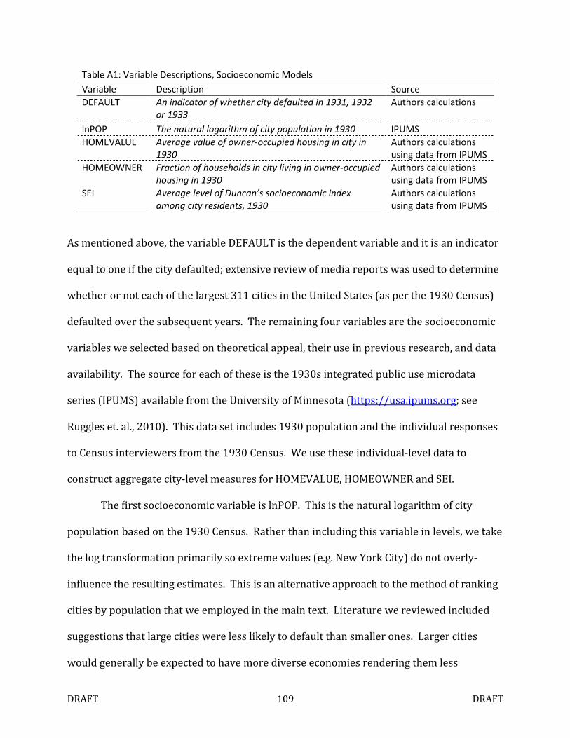
DRAFT 109 DRAFT
Table A1: Variable Descriptions, Socioeconomic Models
Variable Description Source
DEFAULT
An indicator of whether city defaulted in 1931, 1932
or 1933
Authors calculations
lnPOP The natural logarithm of city population in 1930 IPUMS
HOMEVALUE
Average value of owner-occupied housing in city in
1930
Authors calculations
using data from IPUMS
HOMEOWNER
Fraction of households in city living in owner-occupied
housing in 1930
Authors calculations
using data from IPUMS
SEI
Average level of Duncan’s socioeconomic index
among city residents, 1930
Authors calculations
using data from IPUMS
As mentioned above, the variable DEFAULT is the dependent variable and it is an indicator
equal to one if the city defaulted; extensive review of media reports was used to determine
whether or not each of the largest 311 cities in the United States (as per the 1930 Census)
defaulted over the subsequent years. The remaining four variables are the socioeconomic
variables we selected based on theoretical appeal, their use in previous research, and data
availability. The source for each of these is the 1930s integrated public use microdata
series (IPUMS) available from the University of Minnesota (https://usa.ipums.org; see
Ruggles et. al., 2010). This data set includes 1930 population and the individual responses
to Census interviewers from the 1930 Census. We use these individual-level data to
construct aggregate city-level measures for HOMEVALUE, HOMEOWNER and SEI.
The first socioeconomic variable is lnPOP. This is the natural logarithm of city
population based on the 1930 Census. Rather than including this variable in levels, we take
the log transformation primarily so extreme values (e.g. New York City) do not overly-
influence the resulting estimates. This is an alternative approach to the method of ranking
cities by population that we employed in the main text. Literature we reviewed included
suggestions that large cities were less likely to default than smaller ones. Larger cities
would generally be expected to have more diverse economies rendering them less
DRAFT 110 DRAFT
vulnerable to the collapse of any given industry. Also, larger cities may be more able to
attract state or federal bailouts, due to their greater importance and political power. Next,
HOMEVALUE is the average value of owner-occupied housing in the city. We expect that
cities with high values will be less likely to default as property tax revenue will be greater
in these cities allowing governments to more easily service debt.
The variable HOMEOWNER is the fraction of residents that own their home (either
outright or have a mortgage.) It is possible that voters in cities with a high homeownership
rate will pressure politicians to not default, as they are worried that bad publicity resulting
from a default will lower the value of what for most of them is their single largest asset. On
the other hand, if default allows cities to “wipe the slate clean”, it could be in the financial
interest of homeowners for the city to default. Thus determining the effect of
homeownership on default probability is an empirical question. Finally, SEI stands for
socioeconomic index. This particular index is the Duncan SEI and is contained in the IPUMS
data. The 1930 Census did not ask questions about income, and so SEI is the closest
available proxy for income at the city level that is available. Like HOMEVALUE, we expect
that richer cities will be less likely to default, as governments will be able to more easily
raise revenue from richer citizens.
Table A2 below presents summary statistics for these variables. As can be seen, our
sample size is 299, which excludes the eleven cities that defaulted in 1930, 1935 or 1936,
and also Honolulu for which IPUMS data was not available. Twelve percent of cities in this
sample are classified as defaulting. About 46% of citizens were homeowners, and this
value ranged from 22% to 74%. These and other facts about our sample can be seen in the
table below.
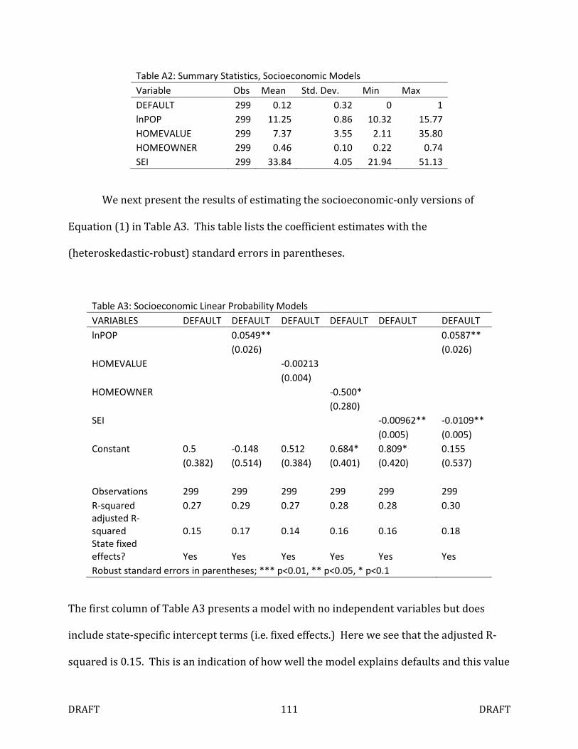
DRAFT 111 DRAFT
Table A2: Summary Statistics, Socioeconomic Models
Variable Obs Mean Std. Dev. Min Max
DEFAULT 299 0.12 0.32 0 1
lnPOP 299 11.25 0.86 10.32 15.77
HOMEVALUE 299 7.37 3.55 2.11 35.80
HOMEOWNER 299 0.46 0.10 0.22 0.74
SEI 299 33.84 4.05 21.94 51.13
We next present the results of estimating the socioeconomic-only versions of
Equation (1) in Table A3. This table lists the coefficient estimates with the
(heteroskedastic-robust) standard errors in parentheses.
Table A3: Socioeconomic Linear Probability Models
VARIABLES DEFAULT DEFAULT DEFAULT DEFAULT DEFAULT DEFAULT
lnPOP
0.0549**
0.0587**
(0.026)
(0.026)
HOMEVALUE
-0.00213
(0.004)
HOMEOWNER
-0.500*
(0.280)
SEI
-0.00962** -0.0109**
(0.005) (0.005)
Constant 0.5 -0.148 0.512 0.684* 0.809* 0.155
(0.382) (0.514) (0.384) (0.401) (0.420) (0.537)
Observations 299 299 299 299 299 299
R-squared 0.27 0.29 0.27 0.28 0.28 0.30
adjusted R-
squared 0.15 0.17 0.14 0.16 0.16 0.18
State fixed
effects? Yes Yes Yes Yes Yes Yes
Robust standard errors in parentheses; *** p<0.01, ** p<0.05, * p<0.1
The first column of Table A3 presents a model with no independent variables but does
include state-specific intercept terms (i.e. fixed effects.) Here we see that the adjusted R-
squared is 0.15. This is an indication of how well the model explains defaults and this value
DRAFT 112 DRAFT
serves as a benchmark for the incremental explanatory power of the independent
variables. In the second column, we see that the coefficient on lnPOP is positive
(suggesting greater default risk with increased population; not the expected sign) which is
significant at the 5% level. The adjusted R2 is 0.17, a slight improvement over the fixed-
effect only specification in column one.
In column three we see that the coefficient on HOMEVALUE is -0.00213. However,
while the sign is consistent with our expectations, the estimate is not statistically
significant. In column four, the coefficient on HOMEOWN is -0.5. The sign is consistent
with a situation where homeowners view defaulting as eroding the value of their single
largest investment, and the estimate is marginally significant. However, as our cutoff value
for including variables in the semi-final model is the 5% level, we consider the estimated
coefficient on HOMEOWN to be statistically insignificant (i.e. we cannot reject the
hypothesis that the true population coefficient is zero with 95% confidence.)
In column five the coefficient on SEI is -0.00962. This estimate is significant at the
5% level. The sign is consistent with our expectations. The adjusted R2 is 0.16, an even
slighter improvement over the fixed-effect only specification in column one then the model
that included only lnPOP.
After reviewing the estimates on each of the coefficients from columns two through
five, we determined that two socioeconomic variables meet the threshold for inclusion in
the socioeconomic-only semi-final model, and we present this in column six. Both
estimates retain their statistical significance, and the magnitudes of the estimates do not
change much. The adjusted R2 increases to 0.18, the highest of any of the models presented
in Table A3. However, this is still a rather modest increase over the fixed-effect model from
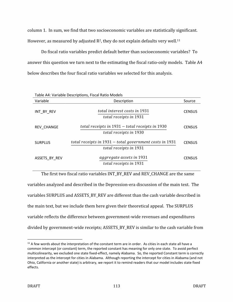
DRAFT 113 DRAFT
column 1. In sum, we find that two socioeconomic variables are statistically significant.
However, as measured by adjusted R2, they do not explain defaults very well.11
Do fiscal ratio variables predict default better than socioeconomic variables? To
answer this question we turn next to the estimating the fiscal ratio-only models. Table A4
below describes the four fiscal ratio variables we selected for this analysis.
Table A4: Variable Descriptions, Fiscal Ratio Models
Variable Description Source
INT_BY_REV
���./�1����2�3�2�2�11931
���./��3��6�2�11931
CENSUS
REV_CHANGE
���./��3��6�2�11931 − ���./��3��6�2�11930
���./��3��6�2�11930
CENSUS
SURPLUS
���./��3��6�2�11931 − ���./9�:��1;�1�3�2�2�11931
���./��3��6�2�11931
CENSUS
ASSETS_BY_REV
.99��9.��.22��2�11931
���./��3��6�2�11931
CENSUS
The first two fiscal ratio variables INT_BY_REV and REV_CHANGE are the same
variables analyzed and described in the Depression-era discussion of the main text. The
variables SURPLUS and ASSETS_BY_REV are different than the cash variable described in
the main text, but we include them here given their theoretical appeal. The SURPLUS
variable reflects the difference between government-wide revenues and expenditures
divided by government-wide receipts; ASSETS_BY_REV is similar to the cash variable from
11 A few words about the interpretation of the constant term are in order. As cities in each state all have a
common intercept (or constant) term, the reported constant has meaning for only one state. To avoid perfect
multicolinearity, we excluded one state fixed-effect, namely Alabama. So, the reported Constant term is correctly
interpreted as the intercept for cities in Alabama. Although reporting the intercept for cities in Alabama (and not
Ohio, California or another state) is arbitrary, we report it to remind readers that our model includes state fixed
effects.
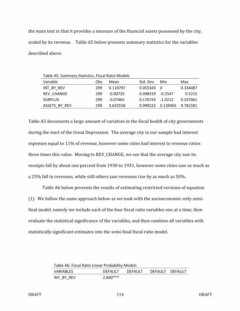
DRAFT 114 DRAFT
the main text in that it provides a measure of the financial assets possessed by the city,
scaled by its revenue. Table A5 below presents summary statistics for the variables
described above.
Table A5: Summary Statistics, Fiscal Ratio Models
Variable Obs Mean Std. Dev. Min Max
INT_BY_REV 299 0.110797 0.055343 0 0.334087
REV_CHANGE 299 -0.00735 0.098319 -0.2547 0.5215
SURPLUS 299 -0.07465 0.176743 -1.0212 0.247061
ASSETS_BY_REV 299 3.632558 0.999222 0.139465 9.781581
Table A5 documents a large amount of variation in the fiscal health of city governments
during the start of the Great Depression. The average city in our sample had interest
expenses equal to 11% of revenue, however some cities had interest to revenue ratios
three times this value. Moving to REV_CHANGE, we see that the average city saw its
receipts fall by about one percent from 1930 to 1931, however some cities saw as much as
a 25% fall in revenues, while still others saw revenues rise by as much as 50%.
Table A6 below presents the results of estimating restricted versions of equation
(1). We follow the same approach below as we took with the socioeconomic-only semi-
final model, namely we include each of the four fiscal ratio variables one at a time, then
evaluate the statistical significance of the variables, and then combine all variables with
statistically significant estimates into the semi-final fiscal ratio model.
Table A6: Fiscal Ratio Linear Probability Models
VARIABLES DEFAULT DEFAULT DEFAULT DEFAULT
INT_BY_REV 2.840***
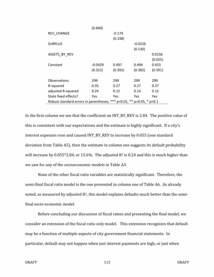
DRAFT 115 DRAFT
(0.600)
REV_CHANGE
-0.174
(0.198)
SURPLUS
-0.0226
(0.130)
ASSETS_BY_REV
0.0156
(0.025)
Constant -0.0429 0.497 0.494 0.433
(0.322) (0.392) (0.382) (0.391)
Observations 299 299 299 299
R-squared 0.35 0.27 0.27 0.27
adjusted R-squared 0.24 0.15 0.14 0.15
State fixed effects? Yes Yes Yes Yes
Robust standard errors in parentheses; *** p<0.01, ** p<0.05, * p<0.1
In the first column we see that the coefficient on INT_BY_REV is 2.84. The positive value of
this is consistent with our expectations and the estimate is highly significant. If a city’s
interest expenses rose and caused INT_BY_REV to increase by 0.055 (one standard
deviation from Table A5), then the estimate in column one suggests its default probability
will increase by 0.055*2.84, or 15.6%. The adjusted R2 is 0.24 and this is much higher than
we saw for any of the socioeconomic models in Table A3.
None of the other fiscal ratio variables are statistically significant. Therefore, the
semi-final fiscal ratio model is the one presented in column one of Table A6. As already
noted, as measured by adjusted R2, this model explains defaults much better than the semi-
final socio-economic model.
Before concluding our discussion of fiscal ratios and presenting the final model, we
consider an extension of the fiscal ratio only model. This extension recognizes that default
may be a function of multiple aspects of city government financial statements. In
particular, default may not happen when just interest payments are high, or just when
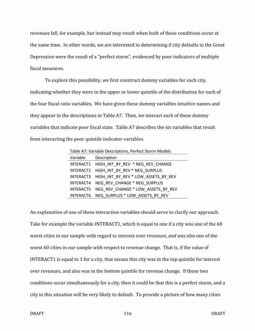
DRAFT 116 DRAFT
revenues fall, for example, but instead may result when both of these conditions occur at
the same time. In other words, we are interested in determining if city defaults in the Great
Depression were the result of a “perfect storm”, evidenced by poor indicators of multiple
fiscal measures.
To explore this possibility, we first construct dummy variables for each city,
indicating whether they were in the upper or lower quintile of the distribution for each of
the four fiscal ratio variables. We have given these dummy variables intuitive names and
they appear in the descriptions in Table A7. Then, we interact each of these dummy
variables that indicate poor fiscal state. Table A7 describes the six variables that result
from interacting the poor quintile indicator variables.
Table A7: Variable Descriptions, Perfect Storm Models
Variable Description
INTERACT1 HIGH_INT_BY_REV * NEG_REV_CHANGE
INTERACT2 HIGH_INT_BY_REV * NEG_SURPLUS
INTERACT3 HIGH_INT_BY_REV * LOW_ASSETS_BY_REV
INTERACT4 NEG_REV_CHANGE * NEG_SURPLUS
INTERACT5 NEG_REV_CHANGE * LOW_ASSETS_BY_REV
INTERACT6 NEG_SURPLUS * LOW_ASSETS_BY_REV
An explanation of one of these interaction variables should serve to clarify our approach.
Take for example the variable INTERACT1, which is equal to one if a city was one of the 60
worst cities in our sample with regard to interest over revenues, and was also one of the
worst 60 cities in our sample with respect to revenue change. That is, if the value of
INTERACT1 is equal to 1 for a city, that means this city was in the top quintile for interest
over revenues, and also was in the bottom quintile for revenue change. If these two
conditions occur simultaneously for a city, then it could be that this is a perfect storm, and a
city in this situation will be very likely to default. To provide a picture of how many cities
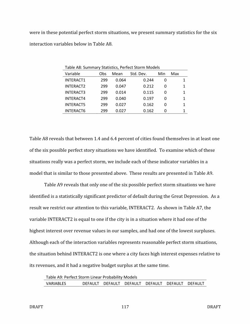
DRAFT 117 DRAFT
were in these potential perfect storm situations, we present summary statistics for the six
interaction variables below in Table A8.
Table A8: Summary Statistics, Perfect Storm Models
Variable Obs Mean Std. Dev. Min Max
INTERACT1 299 0.064 0.244 0 1
INTERACT2 299 0.047 0.212 0 1
INTERACT3 299 0.014 0.115 0 1
INTERACT4 299 0.040 0.197 0 1
INTERACT5 299 0.027 0.162 0 1
INTERACT6 299 0.027 0.162 0 1
Table A8 reveals that between 1.4 and 6.4 percent of cities found themselves in at least one
of the six possible perfect story situations we have identified. To examine which of these
situations really was a perfect storm, we include each of these indicator variables in a
model that is similar to those presented above. These results are presented in Table A9.
Table A9 reveals that only one of the six possible perfect storm situations we have
identified is a statistically significant predictor of default during the Great Depression. As a
result we restrict our attention to this variable, INTERACT2. As shown in Table A7, the
variable INTERACT2 is equal to one if the city is in a situation where it had one of the
highest interest over revenue values in our samples, and had one of the lowest surpluses.
Although each of the interaction variables represents reasonable perfect storm situations,
the situation behind INTERACT2 is one where a city faces high interest expenses relative to
its revenues, and it had a negative budget surplus at the same time.
Table A9: Perfect Storm Linear Probability Models
VARIABLES DEFAULT DEFAULT DEFAULT DEFAULT DEFAULT DEFAULT
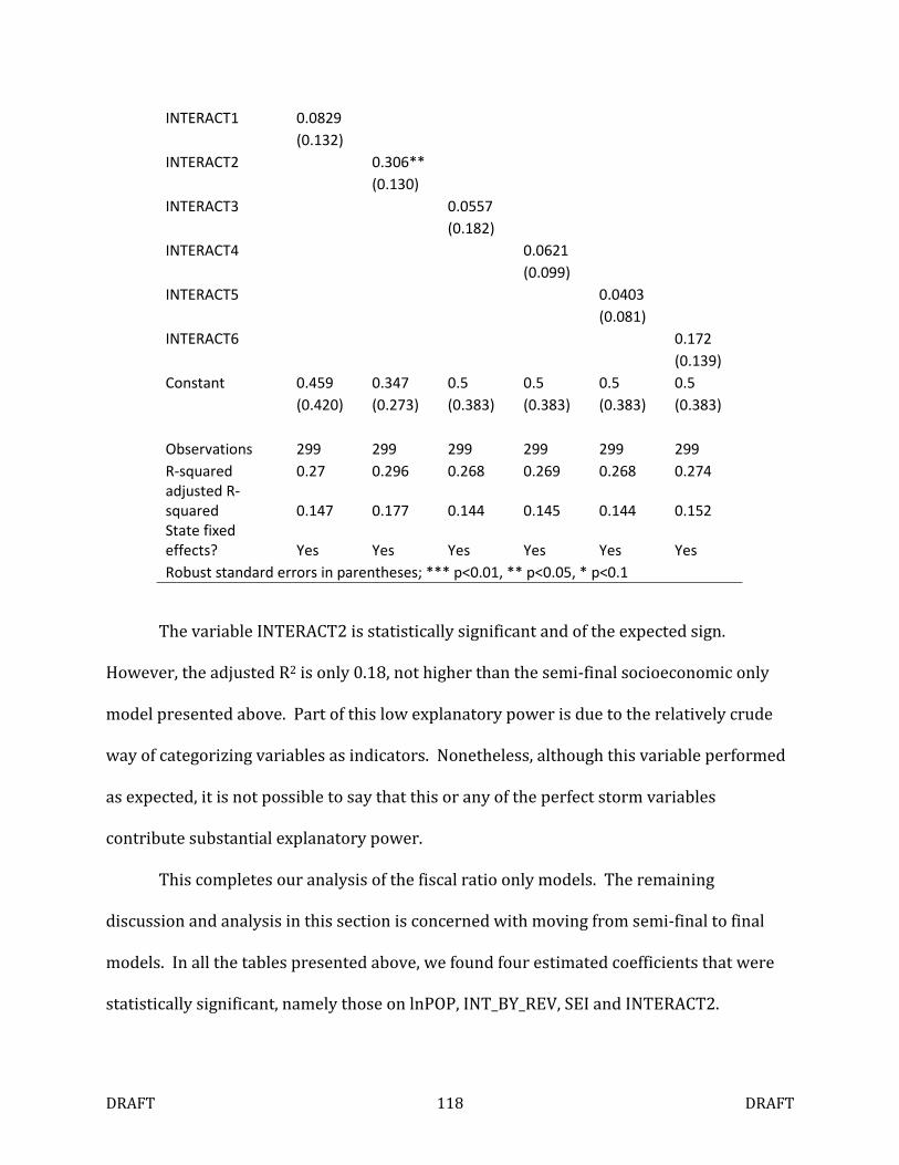
DRAFT 118 DRAFT
INTERACT1 0.0829
(0.132)
INTERACT2
0.306**
(0.130)
INTERACT3
0.0557
(0.182)
INTERACT4
0.0621
(0.099)
INTERACT5
0.0403
(0.081)
INTERACT6
0.172
(0.139)
Constant 0.459 0.347 0.5 0.5 0.5 0.5
(0.420) (0.273) (0.383) (0.383) (0.383) (0.383)
Observations 299 299 299 299 299 299
R-squared 0.27 0.296 0.268 0.269 0.268 0.274
adjusted R-
squared 0.147 0.177 0.144 0.145 0.144 0.152
State fixed
effects? Yes Yes Yes Yes Yes Yes
Robust standard errors in parentheses; *** p<0.01, ** p<0.05, * p<0.1
The variable INTERACT2 is statistically significant and of the expected sign.
However, the adjusted R2 is only 0.18, not higher than the semi-final socioeconomic only
model presented above. Part of this low explanatory power is due to the relatively crude
way of categorizing variables as indicators. Nonetheless, although this variable performed
as expected, it is not possible to say that this or any of the perfect storm variables
contribute substantial explanatory power.
This completes our analysis of the fiscal ratio only models. The remaining
discussion and analysis in this section is concerned with moving from semi-final to final
models. In all the tables presented above, we found four estimated coefficients that were
statistically significant, namely those on lnPOP, INT_BY_REV, SEI and INTERACT2.
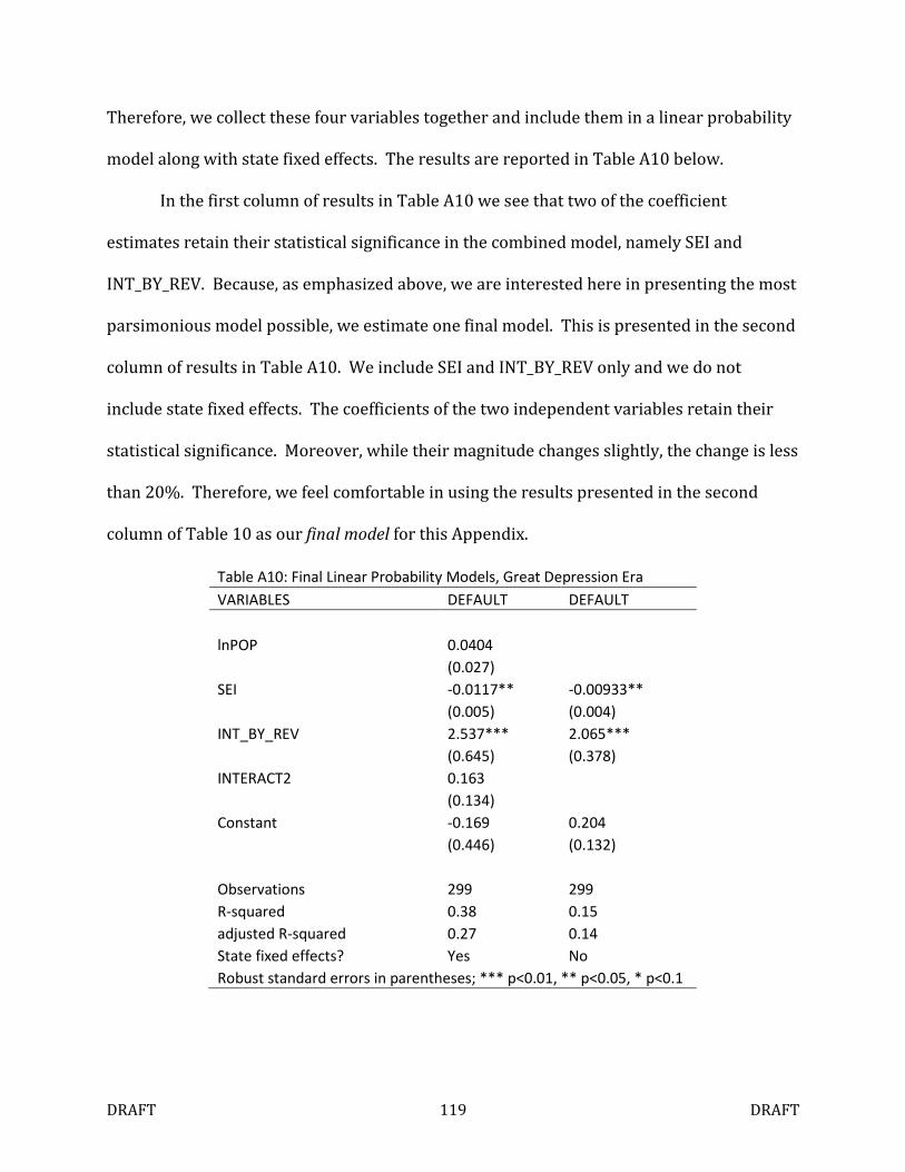
DRAFT 119 DRAFT
Therefore, we collect these four variables together and include them in a linear probability
model along with state fixed effects. The results are reported in Table A10 below.
In the first column of results in Table A10 we see that two of the coefficient
estimates retain their statistical significance in the combined model, namely SEI and
INT_BY_REV. Because, as emphasized above, we are interested here in presenting the most
parsimonious model possible, we estimate one final model. This is presented in the second
column of results in Table A10. We include SEI and INT_BY_REV only and we do not
include state fixed effects. The coefficients of the two independent variables retain their
statistical significance. Moreover, while their magnitude changes slightly, the change is less
than 20%. Therefore, we feel comfortable in using the results presented in the second
column of Table 10 as our final model for this Appendix.
Table A10: Final Linear Probability Models, Great Depression Era
VARIABLES DEFAULT DEFAULT
lnPOP 0.0404
(0.027)
SEI -0.0117** -0.00933**
(0.005) (0.004)
INT_BY_REV 2.537*** 2.065***
(0.645) (0.378)
INTERACT2 0.163
(0.134)
Constant -0.169 0.204
(0.446) (0.132)
Observations 299 299
R-squared 0.38 0.15
adjusted R-squared 0.27 0.14
State fixed effects? Yes No
Robust standard errors in parentheses; *** p<0.01, ** p<0.05, * p<0.1
DRAFT 120 DRAFT
We have used this final model to predict current-era defaults as an alternative to the hybrid
model described in the main text. The equation below presents the model from the second
column of Table 10 in equation format:
����� = 0.204 − 0.00933 ∗ >�? + 2.065 ∗ ?B�_DE_F�G
We used this equation to predict current-period defaults, by plugging in the interest
divided by revenue variable from the 2011 CAFR data set described in this report.
Although Duncan’s SEI index is not available for these cities in 2010, we use median family
income in its place. Data on median family income for cities is taken from the 2009-2011
three year estimates from American Community Survey. To make median family income
more comparable to Depression-era SEI values, we divide by 2,000.
Using this equation to predict current-period defaults allows us to shed light on the
extent to which we should have confidence in the ability of a historical model that only
relies on statistical evidence to predict future defaults. To do this we make use of the 2012
defaults by San Bernardino and Stockton; if this model is able to predict defaults in these
cities, or at least if our model could have indicated that these cities were at risk based on
2011 data, then one can have confidence that the model can be used as the basis for
predicting future defaults.
Would this analysis have predicted defaults in Stockton and San Bernardino? Table
A11 below describes the location of these two defaulting cites in the default likelihood
ranking produced by following the procedure described above. Table A11 is divided into
quintiles, which we have labeled Very safe, Safe, Moderately safe, At risk and Highly at risk.
Our model did a fairly good job of placing San Bernardino, as our rankings put it in the
“Highly at risk” category. Only 30 cities were predicted to be more likely to default than
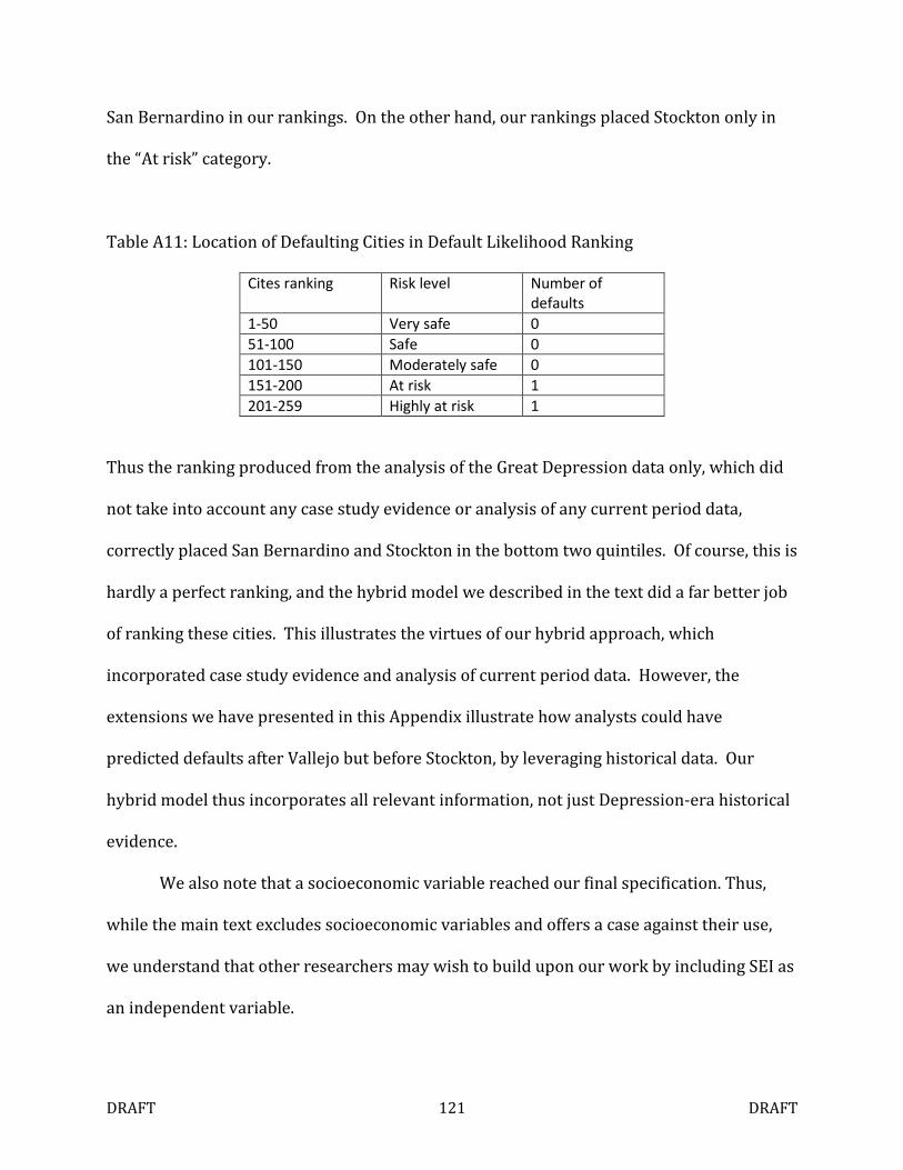
DRAFT 121 DRAFT
San Bernardino in our rankings. On the other hand, our rankings placed Stockton only in
the “At risk” category.
Table A11: Location of Defaulting Cities in Default Likelihood Ranking
Cites ranking Risk level Number of
defaults
1-50 Very safe 0
51-100 Safe 0
101-150 Moderately safe 0
151-200 At risk 1
201-259 Highly at risk 1
Thus the ranking produced from the analysis of the Great Depression data only, which did
not take into account any case study evidence or analysis of any current period data,
correctly placed San Bernardino and Stockton in the bottom two quintiles. Of course, this is
hardly a perfect ranking, and the hybrid model we described in the text did a far better job
of ranking these cities. This illustrates the virtues of our hybrid approach, which
incorporated case study evidence and analysis of current period data. However, the
extensions we have presented in this Appendix illustrate how analysts could have
predicted defaults after Vallejo but before Stockton, by leveraging historical data. Our
hybrid model thus incorporates all relevant information, not just Depression-era historical
evidence.
We also note that a socioeconomic variable reached our final specification. Thus,
while the main text excludes socioeconomic variables and offers a case against their use,
we understand that other researchers may wish to build upon our work by including SEI as
an independent variable.
DRAFT 122 DRAFT
Appendix 2: Comparing data: CAFRs and the SCO’s Cities Annual
Report
The State Controller’s Office (1912, 2012b) has been collecting fiscal data from all
California cities on an annual basis since 1911 and publishes this data in a document
entitled the Cities Annual Report. Since the report leverages a long established collection
mechanism and cooperation from cities is legally mandated, it could theoretically serve as
the data source for a default probability modeling tool. Unfortunately, some aspects of the
SCO reporting mechanism limit its effectiveness for this purpose.
The report is published shortly after September 1 on a one year lag. Since the data
pertain to the fiscal year ending June 30, the report becomes available at least 14 months
after the year closes. For example, data as of June 30, 2012 will be available around
September 1, 2013. By contrast, CAFRs for the last fiscal year began appearing in late 2012,
and most were available by the end of April 2013.
On the other hand, some cities file audited financials on a very long delay. As of April
2013, the City of Adelanto had yet to publish any CAFR more recent than 2008, while
Maywood’s most recent audited financials were as of 2009. Both of these cities did provide
2011 fiscal data for the SCO report. At the same time, Cities Annual Report coverage for
2011 is also incomplete. The cities of Beaumont, Hawthorne, La Habra and Stockton did not
provide SCO with 2011 financial data.
Another concern is that the Cities Annual Report data are collected through a
process separate from that used to create the city’s audited financials. City finance
personnel enter data into a custom data collection instrument provided by SCO. Since the
reporting process is divorced from the CAFR filing, the data may not be consistent.
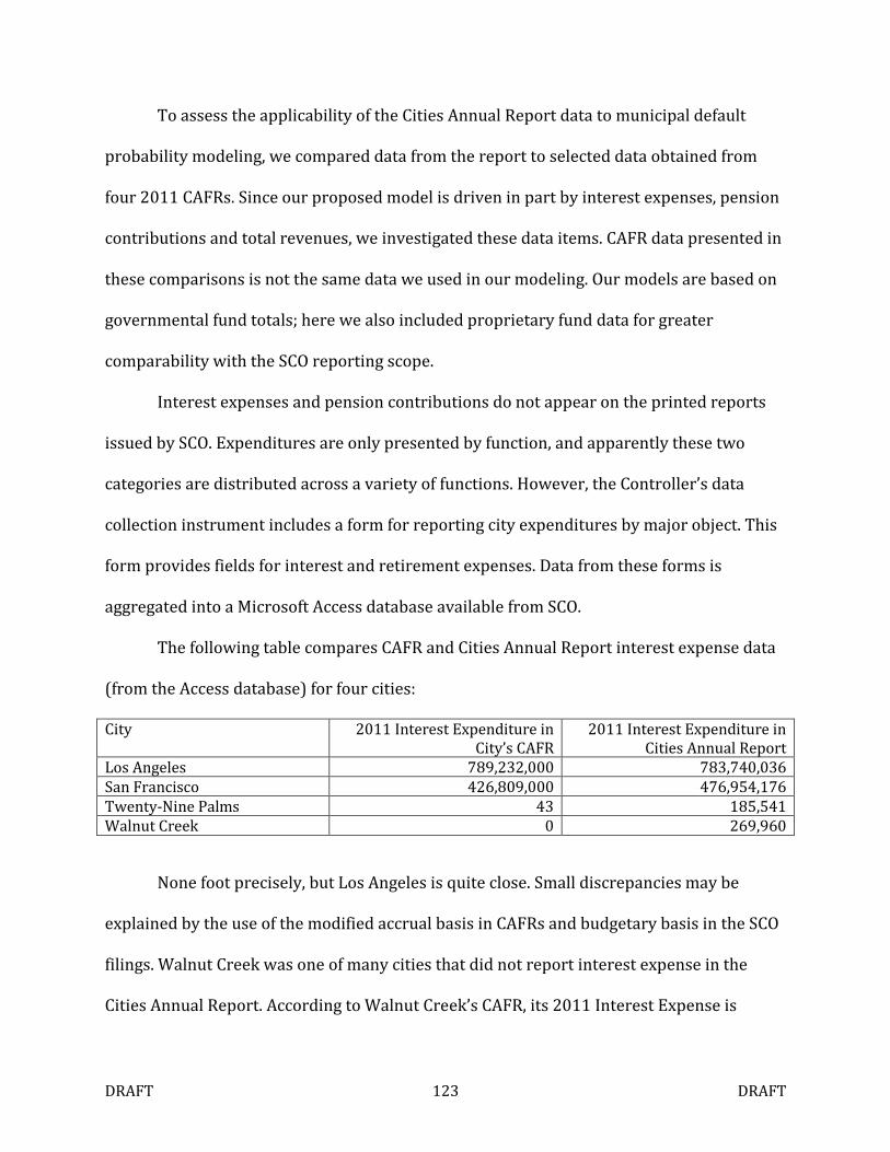
DRAFT 123 DRAFT
To assess the applicability of the Cities Annual Report data to municipal default
probability modeling, we compared data from the report to selected data obtained from
four 2011 CAFRs. Since our proposed model is driven in part by interest expenses, pension
contributions and total revenues, we investigated these data items. CAFR data presented in
these comparisons is not the same data we used in our modeling. Our models are based on
governmental fund totals; here we also included proprietary fund data for greater
comparability with the SCO reporting scope.
Interest expenses and pension contributions do not appear on the printed reports
issued by SCO. Expenditures are only presented by function, and apparently these two
categories are distributed across a variety of functions. However, the Controller’s data
collection instrument includes a form for reporting city expenditures by major object. This
form provides fields for interest and retirement expenses. Data from these forms is
aggregated into a Microsoft Access database available from SCO.
The following table compares CAFR and Cities Annual Report interest expense data
(from the Access database) for four cities:
City 2011 Interest Expenditure in City’s CAFR
2011 Interest Expenditure in Cities Annual Report
Los Angeles 789,232,000 783,740,036
San Francisco 426,809,000 476,954,176
Twenty-Nine Palms 43 185,541
Walnut Creek 0 269,960
None foot precisely, but Los Angeles is quite close. Small discrepancies may be
explained by the use of the modified accrual basis in CAFRs and budgetary basis in the SCO
filings. Walnut Creek was one of many cities that did not report interest expense in the
Cities Annual Report. According to Walnut Creek’s CAFR, its 2011 Interest Expense is
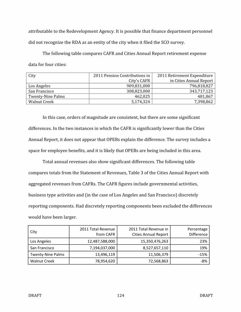
DRAFT 124 DRAFT
attributable to the Redevelopment Agency. It is possible that finance department personnel
did not recognize the RDA as an entity of the city when it filed the SCO survey.
The following table compares CAFR and Cities Annual Report retirement expense
data for four cities:
City 2011 Pension Contributions in City’s CAFR
2011 Retirement Expenditure in Cities Annual Report
Los Angeles 909,831,000 796,818,827
San Francisco 308,823,000 343,717,123
Twenty-Nine Palms 462,025 481,867
Walnut Creek 5,174,324 7,398,862
In this case, orders of magnitude are consistent, but there are some significant
differences. In the two instances in which the CAFR is significantly lower than the Cities
Annual Report, it does not appear that OPEBs explain the difference. The survey includes a
space for employee benefits, and it is likely that OPEBs are being included in this area.
Total annual revenues also show significant differences. The following table
compares totals from the Statement of Revenues, Table 3 of the Cities Annual Report with
aggregated revenues from CAFRs. The CAFR figures include governmental activities,
business type activities and (in the case of Los Angeles and San Francisco) discretely
reporting components. Had discretely reporting components been excluded the differences
would have been larger.
City 2011 Total Revenue
from CAFR
2011 Total Revenue in
Cities Annual Report
Percentage
Difference
Los Angeles 12,487,588,000 15,350,476,263 23%
San Francisco 7,194,037,000 8,527,657,110 19%
Twenty-Nine Palms 13,496,119 11,506,379 -15%
Walnut Creek 78,954,620 72,568,863 -8%
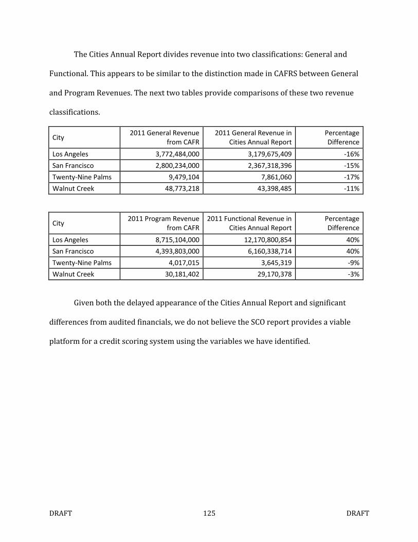
DRAFT 125 DRAFT
The Cities Annual Report divides revenue into two classifications: General and
Functional. This appears to be similar to the distinction made in CAFRS between General
and Program Revenues. The next two tables provide comparisons of these two revenue
classifications.
City 2011 General Revenue
from CAFR
2011 General Revenue in
Cities Annual Report
Percentage
Difference
Los Angeles 3,772,484,000 3,179,675,409 -16%
San Francisco 2,800,234,000 2,367,318,396 -15%
Twenty-Nine Palms 9,479,104 7,861,060 -17%
Walnut Creek 48,773,218 43,398,485 -11%
City 2011 Program Revenue
from CAFR
2011 Functional Revenue in
Cities Annual Report
Percentage
Difference
Los Angeles 8,715,104,000 12,170,800,854 40%
San Francisco 4,393,803,000 6,160,338,714 40%
Twenty-Nine Palms 4,017,015 3,645,319 -9%
Walnut Creek 30,181,402 29,170,378 -3%
Given both the delayed appearance of the Cities Annual Report and significant
differences from audited financials, we do not believe the SCO report provides a viable
platform for a credit scoring system using the variables we have identified.
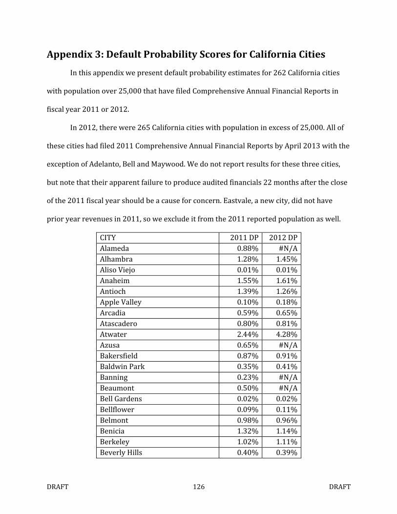
DRAFT 126 DRAFT
Appendix 3: Default Probability Scores for California Cities
In this appendix we present default probability estimates for 262 California cities
with population over 25,000 that have filed Comprehensive Annual Financial Reports in
fiscal year 2011 or 2012.
In 2012, there were 265 California cities with population in excess of 25,000. All of
these cities had filed 2011 Comprehensive Annual Financial Reports by April 2013 with the
exception of Adelanto, Bell and Maywood. We do not report results for these three cities,
but note that their apparent failure to produce audited financials 22 months after the close
of the 2011 fiscal year should be a cause for concern. Eastvale, a new city, did not have
prior year revenues in 2011, so we exclude it from the 2011 reported population as well.
CITY 2011 DP 2012 DP
Alameda 0.88% #N/A
Alhambra 1.28% 1.45%
Aliso Viejo 0.01% 0.01%
Anaheim 1.55% 1.61%
Antioch 1.39% 1.26%
Apple Valley 0.10% 0.18%
Arcadia 0.59% 0.65%
Atascadero 0.80% 0.81%
Atwater 2.44% 4.28%
Azusa 0.65% #N/A
Bakersfield 0.87% 0.91%
Baldwin Park 0.35% 0.41%
Banning 0.23% #N/A
Beaumont 0.50% #N/A
Bell Gardens 0.02% 0.02%
Bellflower 0.09% 0.11%
Belmont 0.98% 0.96%
Benicia 1.32% 1.14%
Berkeley 1.02% 1.11%
Beverly Hills 0.40% 0.39%
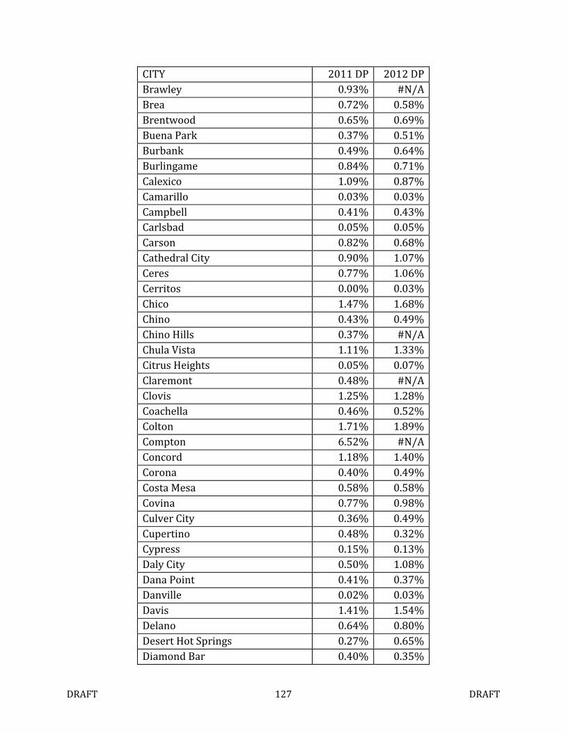
DRAFT 127 DRAFT
CITY 2011 DP 2012 DP
Brawley 0.93% #N/A
Brea 0.72% 0.58%
Brentwood 0.65% 0.69%
Buena Park 0.37% 0.51%
Burbank 0.49% 0.64%
Burlingame 0.84% 0.71%
Calexico 1.09% 0.87%
Camarillo 0.03% 0.03%
Campbell 0.41% 0.43%
Carlsbad 0.05% 0.05%
Carson 0.82% 0.68%
Cathedral City 0.90% 1.07%
Ceres 0.77% 1.06%
Cerritos 0.00% 0.03%
Chico 1.47% 1.68%
Chino 0.43% 0.49%
Chino Hills 0.37% #N/A
Chula Vista 1.11% 1.33%
Citrus Heights 0.05% 0.07%
Claremont 0.48% #N/A
Clovis 1.25% 1.28%
Coachella 0.46% 0.52%
Colton 1.71% 1.89%
Compton 6.52% #N/A
Concord 1.18% 1.40%
Corona 0.40% 0.49%
Costa Mesa 0.58% 0.58%
Covina 0.77% 0.98%
Culver City 0.36% 0.49%
Cupertino 0.48% 0.32%
Cypress 0.15% 0.13%
Daly City 0.50% 1.08%
Dana Point 0.41% 0.37%
Danville 0.02% 0.03%
Davis 1.41% 1.54%
Delano 0.64% 0.80%
Desert Hot Springs 0.27% 0.65%
Diamond Bar 0.40% 0.35%
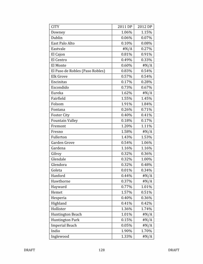
DRAFT 128 DRAFT
CITY 2011 DP 2012 DP
Downey 1.06% 1.15%
Dublin 0.06% 0.07%
East Palo Alto 0.10% 0.08%
Eastvale #N/A 0.27%
El Cajon 0.81% 0.91%
El Centro 0.49% 0.33%
El Monte 0.60% #N/A
El Paso de Robles (Paso Robles) 0.83% 0.54%
Elk Grove 0.57% 0.54%
Encinitas 0.17% 0.28%
Escondido 0.73% 0.67%
Eureka 1.62% #N/A
Fairfield 1.55% 1.45%
Folsom 1.91% 1.84%
Fontana 0.26% 0.71%
Foster City 0.40% 0.41%
Fountain Valley 0.18% 0.17%
Fremont 1.20% 1.11%
Fresno 1.58% #N/A
Fullerton 1.43% 1.53%
Garden Grove 0.54% 1.06%
Gardena 1.16% 1.16%
Gilroy 0.32% 0.36%
Glendale 0.32% 1.00%
Glendora 0.32% 0.48%
Goleta 0.01% 0.34%
Hanford 0.44% #N/A
Hawthorne 0.37% #N/A
Hayward 0.77% 1.01%
Hemet 1.57% 0.51%
Hesperia 0.40% 0.36%
Highland 0.41% 0.42%
Hollister 1.36% 1.74%
Huntington Beach 1.01% #N/A
Huntington Park 0.15% #N/A
Imperial Beach 0.05% #N/A
Indio 1.90% 1.70%
Inglewood 1.33% #N/A
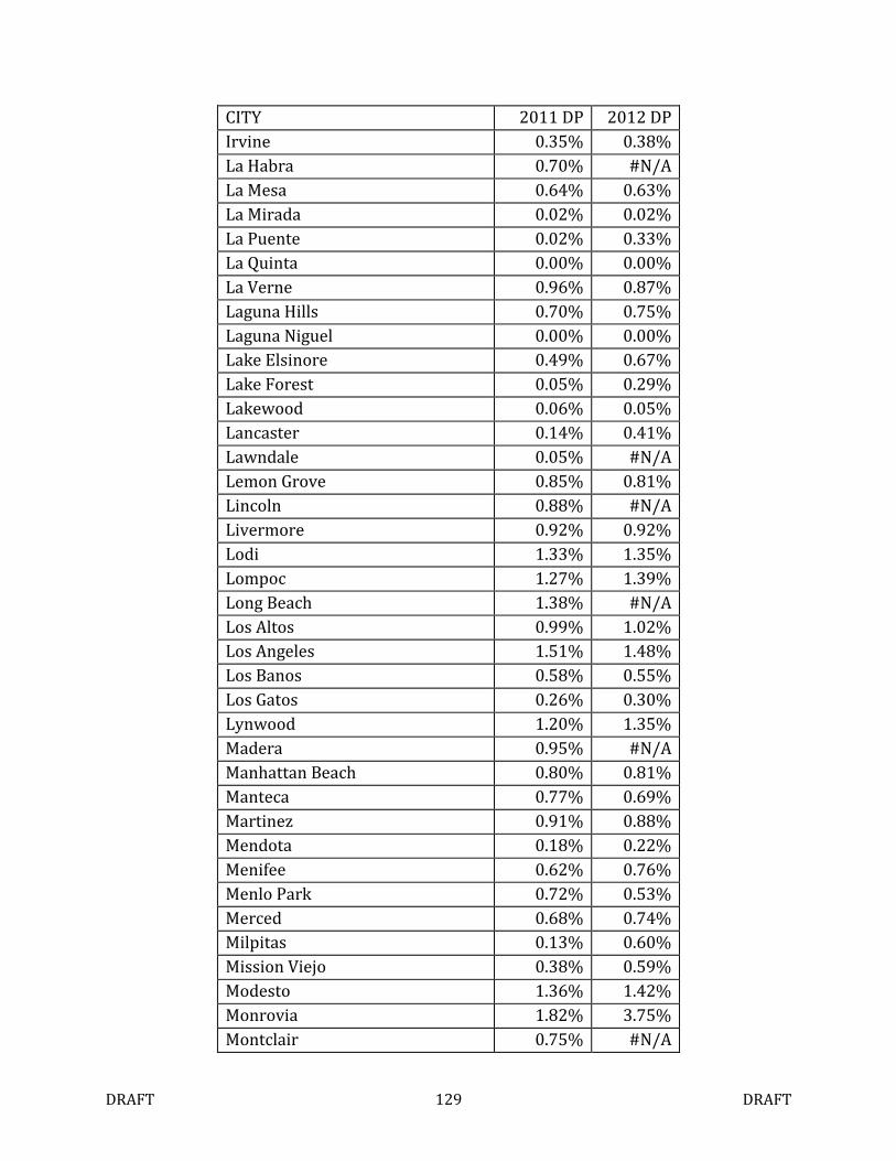
DRAFT 129 DRAFT
CITY 2011 DP 2012 DP
Irvine 0.35% 0.38%
La Habra 0.70% #N/A
La Mesa 0.64% 0.63%
La Mirada 0.02% 0.02%
La Puente 0.02% 0.33%
La Quinta 0.00% 0.00%
La Verne 0.96% 0.87%
Laguna Hills 0.70% 0.75%
Laguna Niguel 0.00% 0.00%
Lake Elsinore 0.49% 0.67%
Lake Forest 0.05% 0.29%
Lakewood 0.06% 0.05%
Lancaster 0.14% 0.41%
Lawndale 0.05% #N/A
Lemon Grove 0.85% 0.81%
Lincoln 0.88% #N/A
Livermore 0.92% 0.92%
Lodi 1.33% 1.35%
Lompoc 1.27% 1.39%
Long Beach 1.38% #N/A
Los Altos 0.99% 1.02%
Los Angeles 1.51% 1.48%
Los Banos 0.58% 0.55%
Los Gatos 0.26% 0.30%
Lynwood 1.20% 1.35%
Madera 0.95% #N/A
Manhattan Beach 0.80% 0.81%
Manteca 0.77% 0.69%
Martinez 0.91% 0.88%
Mendota 0.18% 0.22%
Menifee 0.62% 0.76%
Menlo Park 0.72% 0.53%
Merced 0.68% 0.74%
Milpitas 0.13% 0.60%
Mission Viejo 0.38% 0.59%
Modesto 1.36% 1.42%
Monrovia 1.82% 3.75%
Montclair 0.75% #N/A
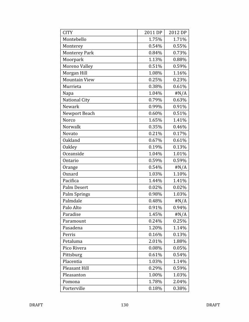
DRAFT 130 DRAFT
CITY 2011 DP 2012 DP
Montebello 1.75% 1.71%
Monterey 0.54% 0.55%
Monterey Park 0.84% 0.73%
Moorpark 1.13% 0.88%
Moreno Valley 0.51% 0.59%
Morgan Hill 1.08% 1.16%
Mountain View 0.25% 0.23%
Murrieta 0.38% 0.61%
Napa 1.04% #N/A
National City 0.79% 0.63%
Newark 0.99% 0.91%
Newport Beach 0.60% 0.51%
Norco 1.65% 1.41%
Norwalk 0.35% 0.46%
Novato 0.21% 0.17%
Oakland 0.67% 0.61%
Oakley 0.19% 0.13%
Oceanside 1.04% 1.01%
Ontario 0.59% 0.59%
Orange 0.54% #N/A
Oxnard 1.03% 1.10%
Pacifica 1.44% 1.41%
Palm Desert 0.02% 0.02%
Palm Springs 0.98% 1.03%
Palmdale 0.48% #N/A
Palo Alto 0.91% 0.94%
Paradise 1.45% #N/A
Paramount 0.24% 0.25%
Pasadena 1.20% 1.14%
Perris 0.16% 0.13%
Petaluma 2.01% 1.88%
Pico Rivera 0.08% 0.05%
Pittsburg 0.61% 0.54%
Placentia 1.03% 1.14%
Pleasant Hill 0.29% 0.59%
Pleasanton 1.00% 1.03%
Pomona 1.78% 2.04%
Porterville 0.18% 0.38%
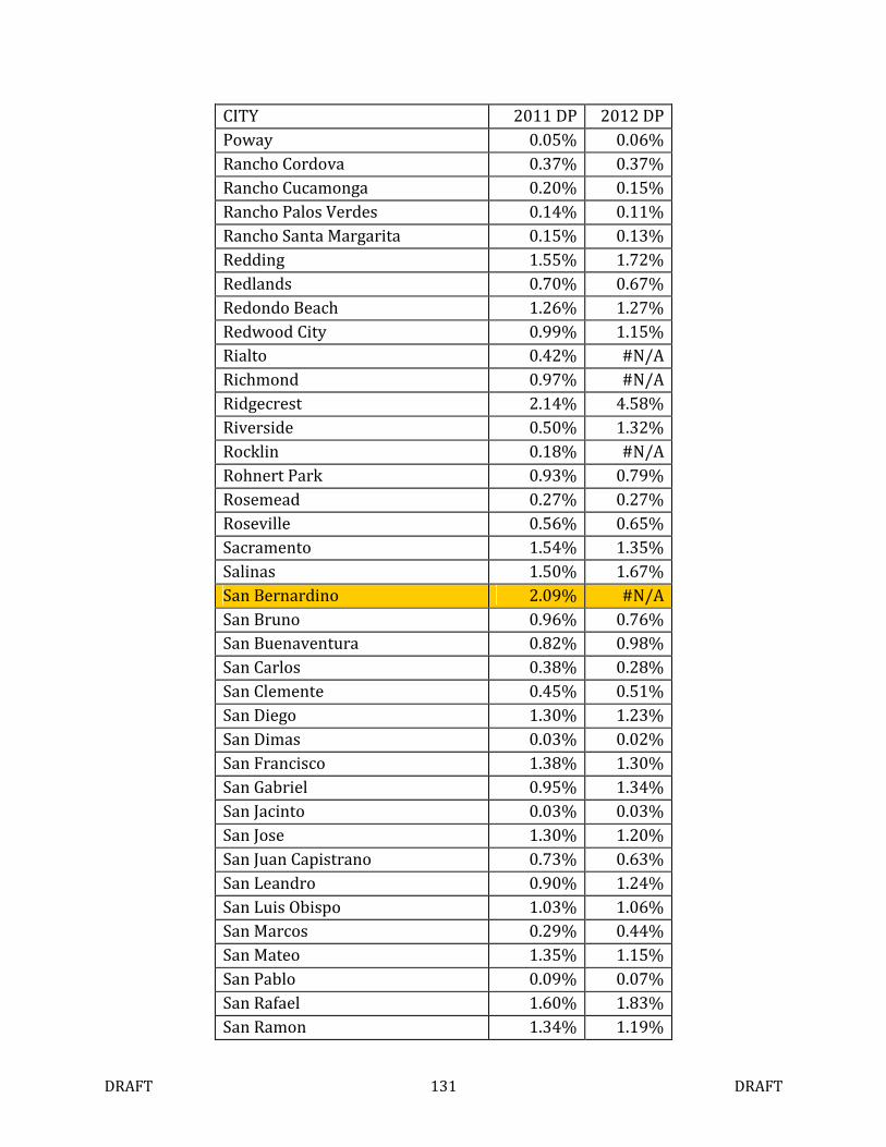
DRAFT 131 DRAFT
CITY 2011 DP 2012 DP
Poway 0.05% 0.06%
Rancho Cordova 0.37% 0.37%
Rancho Cucamonga 0.20% 0.15%
Rancho Palos Verdes 0.14% 0.11%
Rancho Santa Margarita 0.15% 0.13%
Redding 1.55% 1.72%
Redlands 0.70% 0.67%
Redondo Beach 1.26% 1.27%
Redwood City 0.99% 1.15%
Rialto 0.42% #N/A
Richmond 0.97% #N/A
Ridgecrest 2.14% 4.58%
Riverside 0.50% 1.32%
Rocklin 0.18% #N/A
Rohnert Park 0.93% 0.79%
Rosemead 0.27% 0.27%
Roseville 0.56% 0.65%
Sacramento 1.54% 1.35%
Salinas 1.50% 1.67%
San Bernardino 2.09% #N/A
San Bruno 0.96% 0.76%
San Buenaventura 0.82% 0.98%
San Carlos 0.38% 0.28%
San Clemente 0.45% 0.51%
San Diego 1.30% 1.23%
San Dimas 0.03% 0.02%
San Francisco 1.38% 1.30%
San Gabriel 0.95% 1.34%
San Jacinto 0.03% 0.03%
San Jose 1.30% 1.20%
San Juan Capistrano 0.73% 0.63%
San Leandro 0.90% 1.24%
San Luis Obispo 1.03% 1.06%
San Marcos 0.29% 0.44%
San Mateo 1.35% 1.15%
San Pablo 0.09% 0.07%
San Rafael 1.60% 1.83%
San Ramon 1.34% 1.19%
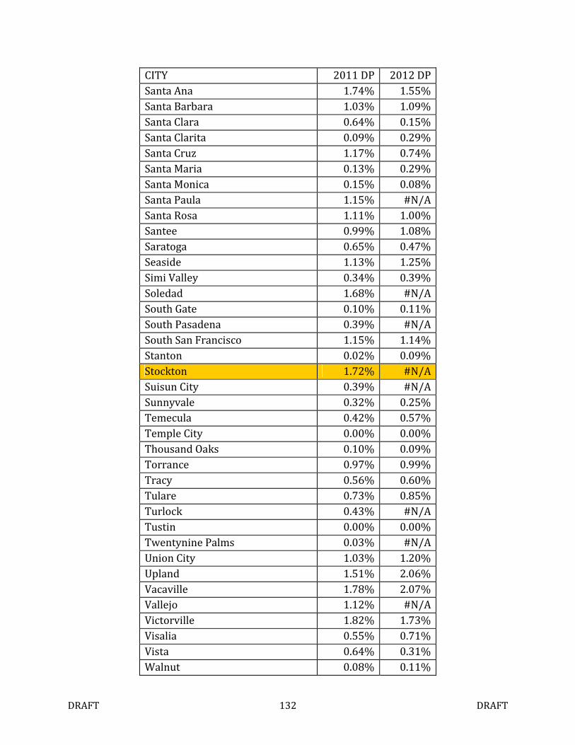
DRAFT 132 DRAFT
CITY 2011 DP 2012 DP
Santa Ana 1.74% 1.55%
Santa Barbara 1.03% 1.09%
Santa Clara 0.64% 0.15%
Santa Clarita 0.09% 0.29%
Santa Cruz 1.17% 0.74%
Santa Maria 0.13% 0.29%
Santa Monica 0.15% 0.08%
Santa Paula 1.15% #N/A
Santa Rosa 1.11% 1.00%
Santee 0.99% 1.08%
Saratoga 0.65% 0.47%
Seaside 1.13% 1.25%
Simi Valley 0.34% 0.39%
Soledad 1.68% #N/A
South Gate 0.10% 0.11%
South Pasadena 0.39% #N/A
South San Francisco 1.15% 1.14%
Stanton 0.02% 0.09%
Stockton 1.72% #N/A
Suisun City 0.39% #N/A
Sunnyvale 0.32% 0.25%
Temecula 0.42% 0.57%
Temple City 0.00% 0.00%
Thousand Oaks 0.10% 0.09%
Torrance 0.97% 0.99%
Tracy 0.56% 0.60%
Tulare 0.73% 0.85%
Turlock 0.43% #N/A
Tustin 0.00% 0.00%
Twentynine Palms 0.03% #N/A
Union City 1.03% 1.20%
Upland 1.51% 2.06%
Vacaville 1.78% 2.07%
Vallejo 1.12% #N/A
Victorville 1.82% 1.73%
Visalia 0.55% 0.71%
Vista 0.64% 0.31%
Walnut 0.08% 0.11%
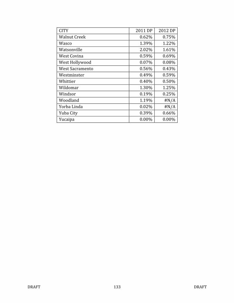
DRAFT 133 DRAFT
CITY 2011 DP 2012 DP
Walnut Creek 0.62% 0.75%
Wasco 1.39% 1.22%
Watsonville 2.02% 1.61%
West Covina 0.59% 0.69%
West Hollywood 0.07% 0.08%
West Sacramento 0.56% 0.43%
Westminster 0.49% 0.59%
Whittier 0.40% 0.50%
Wildomar 1.30% 1.25%
Windsor 0.19% 0.25%
Woodland 1.19% #N/A
Yorba Linda 0.02% #N/A
Yuba City 0.39% 0.66%
Yucaipa 0.00% 0.00%
DRAFT 134 DRAFT
References
Ackerson, E. J. & Chamberlain, J. P. (1935). Legislation and Municipal Debt. Journal of the American
Bar Association, 21, 370-372.
Altman, Brad. (1994, Nov 22). Grand jury questions city manager in review of California city's
defaults. Bond Buyer.
Altman, E. I. and Sabato. G. (2007). Modeling Credit Risk for SMEs: Evidence from the U.S. Market.
Abacus, 43(3), 332-357.
Ameniya, T. (1980). Qualitative Response Models: A Survey. Journal of Economic Literature, 19(4),
1483-1536.
Ang, A. and Green, R, (2011). Lowering Borrowing Costs for States and Municipalities Through
CommonMuni. The Hamilton Project, Brookings Institution. Retrieved 27 August 2012 from
http://www.hamiltonproject.org/files/downloads_and_links/THP_ANG-
GREEN_DiscusPape_Feb2011.pdf.
Beito, David (1989). Taxpayers in Revolt. Chapel Hill, NC: University of North Carolina Press.
Bialaszewski , K. L. (1985). Prediction of Municipal Revenue Bond Default - An Empirical Analysis
Using the Logit Model. Unpublished Dissertation. Mississippi State University.
Bird, Frederick L. (1935). The Municipal Debt Load in 1935: Cities of Over 50,000 Population. New
York: Dun and Bradstreet.
Bird, Frederick L. (1936). The Trend of Tax Delinquency 1930-1935: Cities Over 50,000 Population.
New York: Dun and Bradstreet.
Bohn, J., Arora, N. & Agarwal, D. (2004). Parsimony in Practice: An EDF-Based Model of Credit
Spreads. Moody’s KMV Modeling Methodology Paper.
http://www.moodysanalytics.com/~/media/Insight/Quantitative-Research/Credit-
Valuation/04-29-04-Parsimony-in-Practice.
Bond Buyer and Daily Bond Buyer. Various issues. Now a publication of Source Media, Inc.
DRAFT 135 DRAFT
Buchanan, Wyatt (2012 July 14). Red flags over cities’ bankruptcy filings. San Francisco Chronicle.
http://www.sfgate.com/news/article/Red-flags-over-cities-bankruptcy-filings-
3707978.php#ixzz2Om62Oytt.
Buck, George B. (November 1936). Municipal Pensions. Municipal Finance, 9(2), 17-24.
Bureau of Economic Analysis (2012). Table 1.1.6. Real Gross Domestic Product, Chained Dollars.
http://www.bea.gov/iTable/iTable.cfm?ReqID=9&step=1.
Bureau of Municipal Research (1913). Handbook of Municipal Accounting. New York: D. Appleton
and Company.
Burrill, Donald R. (2011). Servants of the Law: Judicial Politics on the California Frontier, 1849-89: An
Interpretive Exploration of the Field-Terry Controversy. Lanham, MD: University Press of
America.
California Healthline (1998). Healdsburg City Helps Nonprofit Group Buy Hospital.
http://www.californiahealthline.org/articles/1998/10/6/sonoma-county--healdsburg-
city-helps-nonprofit-group-buy-hospital--endstoryhed.aspx.
California State Association of County Auditors (2012). Uniform Guidelines for the Implementation of
Assembly Bill No. 26 of the First Extraordinary Session (ABX1 26) in Connection with the State
of California Budget for Fiscal Year 2011-2012.
http://www.auditorcontroller.org/opencms/about_us/division/Proptax/Redevelopment/
ABx1_26_Guidelinesv10a_Package_2012-05-01.pdf.
California State Constitution (2013). Available at http://www.leginfo.ca.gov/cgi-
bin/waisgate?waisdocid=41929013097+3+0+0&waisaction=retrieve.
CalPERS (2013 April 16). Amortization Periods and Smoothing Methods for Retirement Trust Funds.
http://www.calpers.ca.gov/eip-docs/about/committee-
meetings/agendas/pension/201304/item-9.pdf and http://www.calpers.ca.gov/eip-
docs/about/committee-meetings/agendas/pension/201304/item-9-attach-6.pdf.
DRAFT 136 DRAFT
Carleton, W. T. & Lerner, E. M. (1969). Statistical Credit Scoring of Municipal Bonds. Journal of
Money, Credit and Banking, 1(4), 750-764.
CBS News (2010). State Budgets: The Day of Reckoning. http://www.cbsnews.com/2100-
18560_162-7166220.html?pageNum=4&tag=contentMain;contentBody.
Chalmers, J. M. R. (1998). Default Risk Cannot Explain Muni Puzzle: Evidence from Municipal Bonds
that are Secured by U.S. Treasury Obligations. The Review of Financial Studies, 11(2), 281-
308.
City of Desert Hot Springs (2004). Official Statement: $9,725,000 City of Desert Hot Springs,
Judgment Obligation Bonds. http://emma.msrb.org/MS226949-MS202257-MD392857.pdf.
City of Hercules (2012 November). Monthly Report.
http://www.ci.hercules.ca.us/documents/CM/_Monthly/2012/11-Nov.pdf.
City of Stockton (2013 Mar 25). City of Stockton Chapter 9 Filing – U.S. Bankruptcy Court Proceedings
– Direct Testimony Of City Chief Financial Officer Vanessa Burke In Eligibility Trial.
http://www.stocktongov.com/files/Summary_BurkeTestimony_2013_3_25.pdf
City of Vallejo (2008). Material Event Disclosure Notice.
http://web.archive.org/web/20080924104221/http://www.ci.vallejo.ca.us/uploads/688/
052908%20-%20(05082008)%20-%20Material%20Event%20Disclosure%20Notice.pdf.
City of Vallejo (2011). Comprehensive Annual Financial Report for the Fiscal Year Ended June 30,
2011. http://ci.vallejo.ca.us/common/pages/DisplayFile.aspx?itemId=29331.
Crotty, J. (2011). The Realism of Assumptions Does Matter: Why Keynes-Minsky Theory Must
Replace Efficient Market Theory as the Guide to Financial Regulation Policy. University of
Massachusetts, Amherst Working Paper 2011-05.
http://www.umass.edu/economics/publications/2011-05.pdf.
Dean, Maurice B. (1912). Municipal Bonds Held Void. New York: Moody’s Magazine Book
Department, 1912.
DRAFT 137 DRAFT
Deborah, S. B. (2000 Jun 7). California and the west; voters approve 2 tax measures for desert hot
springs; finance: Without the infusion of cash, the city might have gone bankrupt and seen
its police department dismantled. Los Angeles Times.
Donner, John (1940 Feb). Investment of Pension and Other Trust Funds. Municipal Finance, 12(3),
10-16.
Doty, Robert (2012). Diversity and Risks of Municipal Bonds. Paper presented at The Brandeis
Municipal Finance Conference.
http://www.brandeis.edu/global/pdfs/centers/munifinance/14%20-%20Doty%20-
%20Diversity%20and%20Risks%20of%20Municipal%20Bonds%20.pdf.
Falkenstein, E., Boral, A. and Carty, L. (2000). RiskCalcTM for Private Companies: Moody’s Default
Model. New York: Moody’s Investors Service.
Fama, Eugene (1970). Efficient Capital Markets: A Review of Theory and Empirical Work. The
Journal of Finance, 25(2), 383-417.
Farnham, P. G. and Cluff, G. S. (1984). The Bond Rating Game Revisited: What Information Can Local
Officials Use? Journal of Urban Affairs, 6(4), 21-38.
Faust, Martin L. (1934 Feb). Public Funds in Closed Banks. Municipal Finance, 6(3), 17-19.
Faust, Martin L. (1936). The Security of Public Deposits. Chicago: Public Administration Service.
Fitch Ratings (2012). U.S. Local Government Tax-Supported Rating Criteria.
http://www.fitchratings.com/creditdesk/reports/report_frame.cfm?rpt_id=685314.
Fitch, Inc. (2012). 2012 Form NRSRO Annual Certification Page 128 of 133.
http://www.fitchratings.com/web_content/nrsro/nav/NRSRO_Exhibit-1.pdf.
Fons, Jerome, Randazzo, Thomas and Joffe, Marc. (2011). An Analysis of Historical Municipal Bond
Defaults. New York: Kroll Bond Rating Agency.
Forbes, R. (1973). Quantitative Borrower Characteristics Associated with Defaults on Municipal
General Obligations: Discussion. The Journal of Finance, 28(2), 539-541.
DRAFT 138 DRAFT
Forster, M. & Sober, E. (1994). How to Tell When Simpler, More Unified, or Less Ad Hoc Theories
will Provide More Accurate Predictions. British Journal for the Philosophy of Science, 45, 1-
34.
Garcia, Alex (2013 Mar 7). Council proclaims fiscal emergency. San Fernando Sun.
http://www.sanfernandosun.com/sanfernsun/news/9087-council-proclaims-fiscal-
emergency-.
Gold, S. (2001 Dec 21). The state; resort city files for bankruptcy; finances: Desert hot springs acts
after a judge rules its assets can be seized; civic operations will continue unabated. Los
Angeles Times.
Goodwin Proctor (2011 Feb 9). $30 Million Judgment against Mammoth Lakes for Breach of
Development Agreement. Sustainable Development Blog.
http://www.goodwinsustainabledevelopment.com/uncategorized/30-million-judgment-in-
city%E2%80%99s-breach-of-a-development-agreement/.
Government Accounting Standards Board (2006). Fund balance: It may not be what you think.
http://www.gasb.org/cs/ContentServer?c=GASBContent_C&pagename=GASB%2FGASBCon
tent_C%2FUsersArticlePage&cid=1176156737123.
Governmental Accounting Standards Board (2011). The Timeliness of Financial Reporting by State
and Local Governments Compared with the Needs of Users.
http://www.gasb.org/cs/BlobServer?blobkey=id&blobwhere=1175822186092&blobheade
r=application%2Fpdf&blobcol=urldata&blobtable=MungoBlobs.
Hempel, George H. (1964). The Postwar Quality of Municipal Bonds. Unpublished dissertation.
University of Michigan.
Hempel, George H. (1967). Measures of Municipal Bond Quality. Michigan Business Reports Number
53. Ann Arbor: University of Michigan Graduate School of Business Administration, Bureau
of Business Research.
DRAFT 139 DRAFT
Hempel, George H. (1971). The Post War Quality of State and Local Debt. New York: National Bureau
of Economic Research. http://www.nber.org/chapters/c3424.
Hempel, George H. (1973 Dec.). An Evaluation of Municipal "Bankruptcy" Laws and Procedures. The
Journal of Finance, 28(5), 1339-1351.
Hempel, George H. (1973 May). Quantitative Borrower Characteristics Associated with Defaults on
Municipal General Obligations. The Journal of Finance, 28(2), 523-530.
Hempel, George H. (1975 Oct 6). Testimony before the Subcommittee on Civil and Constitutional
Rights of the House Committee on the Judiciary. 94th Cong.
Hillhouse, A. M. (1935). Defaulted municipal bonds (1830-1930) (Classified list with citations).
Chicago: Municipal Finance Officers Association of the United States and Canada.
Hillhouse, A. M. (1936). Municipal Bonds: A Century of Experience. New York: Prentice Hall.
Hillhouse, Albert M. (1935). Defaulted Municipal Bonds (1830-1930). Chicago: Municipal Finance
Officers’ Association.
Holtzman, Jonathan V., K. Scott Dickey and Steve Cikes (2011). Declarations of Fiscal Emergency: a
Resurging Option for Public Entities Attempting to deal with the Current Economic Climate.
California Public Law Journal, 34(1), 11-13.
Joffe, Marc (2012). Drivers of municipal bond defaults during the Great Depression.
http://papers.ssrn.com/sol3/papers.cfm?abstract_id=2189889. Thesis at San Francisco
State University.
Jones, Carolyn (2008, Feb 21). Vallejo in danger of declaring bankruptcy. San Francisco Chronicle.
http://www.sfgate.com/bayarea/article/Vallejo-in-danger-of-declaring-bankruptcy-
3293747.php.
Kearney, Laila (2012 Mar 14). Court Approves Ambac Settlement Agreement. Pinole-Hercules Patch.
http://pinole-hercules.patch.com/articles/court-approves-ambac-lawsuit-agreement.
DRAFT 140 DRAFT
Keim, Donald B. and Robert T. Stambaugh. (1986). Predicting Returns in Stock and Bond Markets."
Journal of Financial Economics, 17, 357-90.
Kroll Bond Rating Agency (2012). U.S. Local Government General Obligation Rating Methodology.
http://www.krollbondratings.com/show_report/109.
Lennox, C. (1999). Identifying failing companies: a re-evaluation of the logit, probit and DA
approaches. Journal of Economics and Business, 51(4), 347-364.
Lewis, Michael (2011 Nov). California and Bust. Vanity Fair.
http://www.vanityfair.com/business/features/2011/11/michael-lewis-201111.
Longstaff, F., Mithal, S. & Neis, E. (2004). Corporate Yield Spreads: Default Risk or Liquidity? New
Evidence from the Credit-Default Swap Market. National Bureau of Economic Research
Working Paper 10418. http://www.nber.org/papers/w10418.
Loviscek, A. L. & Crowley, F. (1990). What's in a Municipal Bond Rating?" The Financial Review,
25(1), 25-53.
Malkiel, B. G. (2003). The Efficient Market Hypothesis and Its Critics. The Journal of Economic
Perspectives, 17(1), 59-82
Mayer, Susan (2008, Feb 28). Cash Balances by Fund as of 2-28-08. Memo to Vallejo’s Mayor and City
Council.
http://web.archive.org/web/20081113235152/http://www.ci.vallejo.ca.us/uploads/688/
022808%20Cash%20Balances%20by%20fund.pdf.
McFerrin, John B. (1939). Caldwell and Company. Chapel Hill, NC: University of North Carolina Press.
Menard, S. W. (2002). Applied logistic regression analysis. Thousand Oaks, CA: Sage Publishing.
Moody’s Corporation (2012) 2011 Form NRSO Page 25.
http://www.moodys.com/PublishingImages/MCO/NRSRO%202011.pdf. Retrieved 20 July
2012.
DRAFT 141 DRAFT
Moody’s Municipal and Government Securities Manual (Various Years). Now published by Mergent
Corporation, Fort Mill, SC.
Moody’s Investors Service (2009). Rating Methodology: General Obligation Bonds Issued By U.S.
Local Governments. http://wauwatosa.net/DocumentCenter/View/2197.
Moon, C. G. & Stotsky, J. G. (1993). Municipal bond rating analysis: Sample selectivity and
simultaneous equations bias. Regional Science and Urban Economics, 23, 29-50.
Mysak, Joe (2010 Jan 27). Making money in default with munis means only GOs. Bloomberg.
http://www.bloomberg.com/apps/news?pid=newsarchive&sid=aPfhGR1jR8wU.
Munnell, Alicia (2012). State and Local Pensions: What Now? Washington: Brookings Institution
Press.
National Municipal League Consultant Service (1938 Feb 5). The Governments of Atlanta and Fulton
County Georgia: A Summary of the Report of the Administrative and Financial Survey of the
Several Departments and Activities of the City of Atlanta and Fulton County. Atlanta: Atlanta
Chamber of Commerce.
New York State Comptroller’s Office (2013). Fiscal Stress Monitoring System.
http://www.osc.state.ny.us/localgov/pubs/fiscalmonitoring/pdf/fiscalstressmonitoring20
13.pdf.
Ohlson. J.S. (1980). Financial ratios and the probabilistic prediction of bankruptcy. Journal of
Accounting Research 18(1) 109–131.
Palumbo, G. & Zaporowski, M. P. (2012). Determinants of Municipal Bond Ratings for General-
Purpose Governments: An Empirical Analysis. Public Budgeting & Finance, 32(2), 86-102.
Reid, Podkul & McNeill (2012). San Bernardino paid $2 million in cash-outs before bankruptcy
filing. Thomson Reuters Bankruptcy Law News.
http://newsandinsight.thomsonreuters.com/Bankruptcy/News/2012/12_-
DRAFT 142 DRAFT
_December/Exclusive__San_Bernardino_paid_$2_mln_in_cash-
outs_before_bankruptcy_filing/
Reinhart, C. and Rogoff, K. (2009). This Time Is Different. Princeton: Princeton University Press.
Rightor, C. E. (February 1938). New Sources of Municipal Revenue. Municipal Finance, 12(3), 7-10.
Rohrs, Sarah (2008 February 25). Vallejo talks break off, city manager recommends bankruptcy.
The Times Herald. http://www.timesheraldonline.com/todaysnews/ci_8362650.
Rubinfeld, D. (March 1973). Credit Ratings and the Market for General Obligation Municipal Bonds.
National Tax Journal, 26(1), 17-27.
Ruggles, Steven J., Trent Alexander, Katie Genadek, Ronald Goeken, Matthew B. Schroeder, and
Matthew Sobek (2010). Integrated Public Use Microdata Series: Version 5.0 [Machine-
readable database]. Minneapolis, MN: Minnesota Population Center [producer and
distributor], 2010.
Sakolski, Aaron M. (1932). The Great American Land Bubble. New York: Harper and Brothers.
Shafroth, Frank (Various Years). Weekly e-News. George Mason University State & Local
Government Leadership Center.
Shumway T. (2002). Forecasting Bankruptcy More Accurately: A Simple Hazard Model. Journal of
Business, 74(1), 101-124.
Smith, Kevin (2012 July 17). Cities move forward, despite debt obligations. Whittier Daily News.
Standard & Poor’s Corporation (2012a), Form 2011 Form NRSRO, Exhibit 1, Table 58
http://www.standardandpoors.com/servlet/BlobServer?blobheadername3=MDT-
Type&blobcol=urldata&blobtable=MungoBlobs&blobheadervalue2=inline%3B+filename%
3DEX1-1.pdf&blobheadername2=Content-
Disposition&blobheadervalue1=application%2Fpdf&blobkey=id&blobheadername1=conte
nt-type&blobwhere=1244102933947&blobheadervalue3=UTF-8. Overall form NRSRO
available at http://www.standardandpoors.com/ratings/form-nrsro/en/us/.
DRAFT 143 DRAFT
Standard & Poor’s Corporation (2012b). Request for Comment: U.S. Local Governments: Methodology
And Assumptions.
http://www.standardandpoors.com/prot/ratings/articles/en/us/?articleType=HTML&ass
etID=1245330050294.
Standard & Poors (2012a Jul 6). Summary: Mammoth Lakes, California; Appropriations.
http://emma.msrb.org/ER610210-ER473845-ER876887.pdf.
Standard & Poors (2012b Dec 19). Summary: Mammoth Lakes, California; Appropriations.
http://emma.msrb.org/EP726679-EP563793-EP965014.pdf.
State Controller’s Office (1912). Annual Report of the Financial Transactions of Municipalities and
Counties of California for the Year 1911.
http://babel.hathitrust.org/cgi/pt?id=uc1.32106019722252;seq=22;view=1up;num=16
State Controller’s Office (2012a). City of Hercules Review Report: Administrative and Internal
Accounting Controls. http://www.sco.ca.gov/Files-EO/Hercules_Internal_Control.pdf.
State Controller’s Office (2012b). Cities Annual Report. http://www.sco.ca.gov/Files-ARD-
Local/LocRep/1011cities.pdf.
Summers, L. (1986). Does the Stock Market Rationally Reflect Fundamental Values? The Journal of
Finance, 41(3), .591-601.
Taxin, Amy and Hannah Dreier (2012 July 30). California Cities' 'Fiscal Emergency' Put Tax
Questions On The Ballot Faster. The Huffington Post.
http://www.huffingtonpost.com/2012/07/30/california-cities-fiscal-_n_1721540.html.
Taylor, Ronald B. (1982a Nov 26). Town Considering Bankruptcy as Way Out of Debts. Los Angeles
Times.
Taylor, Ronald B. (1982b Dec 17). Town Council Fires 16 of 22 Employees. Los Angeles Times.
The Bond Buyer (Various Dates). Now published by Source Media.
DRAFT 144 DRAFT
The Mountain Democrat (1900 Apr 28). Out of the Woods: City Government Inaugurated. Officers-
Elect Duly Qualify and Enter Upon the Discharge of Their Duties. Page 4.
Tinkham, Geroge H. (1923). The History of San Joaquin California County California with
Biographical Sketches. Los Angeles: Historic Record Company.
Town of Mammoth Lakes (2012a). Plan for the Adjustment of Debts of the Town of Mammoth Lakes
California, July 3, 2012. http://www.ci.mammoth-lakes.ca.us/DocumentCenter/View/3079.
Town of Mammoth Lakes (2012b). Resolution of the Town Council of the Town of Mammoth Lakes,
State of California, Adopting the Restructuring Plan Necessary to Make Payments on a
Settlement with Mammoth Lakes Land Acquisition (MLLA) and Ballas Entities.
http://www.ci.mammoth-lakes.ca.us/documents/3/34/R12-
71_201212181017171109.pdf.
U.S. Bank (2013). Notice of Final Default Distribution. http://emma.msrb.com/ EP738332-
EP573106-EP974494.
US Advisory Commission on Intergovernmental Relations (1973 July). City Financial
Emergencies: The Intergovernmental Dimension. Washington: ACIR.
http://www.library.unt.edu/gpo/acir/Reports/policy/a-42.pdf.
US Advisory Commission on Intergovernmental Relations (1985 Mar). Bankruptcies,
Defaults and Other Local Governmental Financial Emergencies. Washington: ACIR.
http://www.library.unt.edu/gpo/acir/Reports/policy/a-99.pdf.
US Government Accountability Office (2007). State and Local Government Retiree Benefits:
Current Status of Benefit Structures, Protections, and Fiscal Outlook for Funding
Future Costs. http://www.gao.gov/assets/270/267150.pdf
US Census Bureau. Financial Statistics of Cities. Various Years. Washington: Government Printing
Office.
DRAFT 145 DRAFT
US Census Bureau (1932). Financial Statistics of State and Local Governments: 1932. Washington:
Government Printing Office.
US Senate Permanent Subcommittee on Investigations (2011). Wall Street and the Financial Crisis:
Anatomy of a Financial Collapse. Washington: Permanent Subcommittee on Investigations.
Wall Street Journal (1965). Redondo Beach Calif., Misses Interest Due Holders of City’s Harbor
Revenue Bonds. July 2, 1965, p 11.
Wells Fargo (2013). Notice Regarding Debt Service Payment To Holders Of $32,785,000 Stockton
Public Financing Authority Lease Revenue Bonds, Series 2004 (Parking And Capital Projects).
http://emma.msrb.org/ER651578-ER505241-ER907975.pdf.
White, Bobby (2011 May 4). Long Road Out of Bankruptcy. Wall Street Journal.
http://online.wsj.com/article/SB10001424052748704740604576301413521204074.html
White, Bobby (2012 Oct 4). Another California City Struggles with Finances. Wall Street Journal.
http://online.wsj.com/article/SB10000872396390443493304578036781420348220.html
Wu, C. (1991). A Certainty Equivalent Approach to Municipal Bond Default Risk Estimation. The
Journal of Financial Research, 14(3), 241-247.
Wu, C., Wang, J. and Zhang, F. (2006). Liquidity, Default, Taxes and Yields on Municipal Bonds. FEDS
Working Paper No. 2005-35. http://ssrn.com/abstract=687500.
Wulf, Hansen & Company (2003). Official Statement: $8,000,000 Variable Rate Demand Certificates
of Participation (2003 Capital Improvement Project). http://emma.msrb.org/MS215725-
MS191033-MD370927.pdf.
Yinger, J. (2010). Municipal Bond Ratings and Citizens’ Rights. American Law and Economics Review,
12(1), 1-38.
Zmijewski, M. E. (1984). Methodological Issues Related to the Estimation of Financial Distress
Prediction Models. Journal of Accounting Research, 22(1984), 59-82.

DRAFT 146 DRAFT
Zorn, C. (2005). A Solution to Separation in Binary Response Models. Political Analysis, 13(2), 157–
170.


![Cap. 173] Pensions CHAPTER 173. PENSIONS. 173.pdf · Pensions, etc., to cease on bankruptcy. 14. Pensions, etc., may cease on sentence to term of imprisonment. 15. Pensions, etc.,](https://img.pdfslide.net/doc/110x75/5f32c41fe2aa25713c052446/cap-173-pensions-chapter-173-173pdf-pensions-etc-to-cease-on-bankruptcy.jpg)