Embed Size (px)
Citation preview
Optimizing Coverage in 3D Wireless Sensor Networks 189
Optimizing Coverage in 3D Wireless Sensor Networks
Nauman Aslam
X
Optimizing Coverage in 3D Wireless Sensor Networks
Nauman Aslam
Department of Engineering Mathematics and Internetworking Dalhousie University, Halifax, Nova Scotia
Canada, B3J-1Z1
1. Introduction
Recent advances in electronic miniaturization, software engineering and wireless communication technologies have enabled the deployment of low-power sensor nodes that are equipped with an embedded processing unit, memory, power-supply, on-board sensor, radio communication facilities (I. F. Akyildiz, W. Su et al. 2002). An important characteristic of sensor nodes is their ability to sense specific phenomena in a target field and send their data to a central node, called the Base Station/sink, possibly through multihop wireless communication links. Since most data gathering applications are concerned with collection of physical data that is generated in the target area monitored by sensor nodes, therefore coverage becomes a core meaure of performance. A fundamental issue in coverage is the quality of monitoring provided by the network. This quality is usually measured by how well deployed sensors cover a target area. In its simplest form, 1-coverage means that every point inthe target area is monitored at least one sensor. In recent years, the problem of providing sensor coverage has received extensive attention from the research community in the context of 2D sensor networks (Xing, Wang et al. 2005; Zhang and Hou 2005; Bai, Kumar et al. 2006). However, most of the real world sensor network deployments often a follow 3D model. Examples of such deployments are environmental monitoring in forests (Mainwaring, Culler et al. 2002; Szewczyk, Osterweil et al. 2004) where sensor nodes are deployed on trees of different heights in a forest, structural health monitoring of multi-storey buildings (Kim, Pakzad et al. 2006; Lynch and Loh 2006) and underwater surveillance networks (Akyildiz, Pompili et al. 2005). In most cases such deployments follow a model where sensor nodes are placed in large quantities over a target region. Excessive deployment of sensor nodes is often desirable to protect the network from individual node failures. However keeping in mind the energy and bandwidth constraints for most applications, the coverage control problem translates to choosing a set of active nodes that ensure that the target region is sufficiently monitored. Considering the fact that sensors are deployed to interact with the physical phenomenon to gather data, coverage becomes one of the fundamental measures to gauge the service quality provided by the network to the application. Different applications may have
11
www.intechopen.com
Smart Wireless Sensor Networks190
different requirements for coverage. Applications such as forest monitoring, or underwater sensor networks may requires every point in the deployment region to be monitored. This problem is referred to as the area coverage problem (Cardei and Wu 2006). Applications such as intrusion detection may require only coverage of specific points (hot spots) in the deployment region. Thus the solution to the coverage control problem is addressed in the context of application requirements. Another crucial aspect of WSN applications is connectivity that can be defined as the ability of sensor nodes to communicate directly or indirectly with any other active node. Typical deployments of WSNs assume sensor nodes communicate with their neighbors to forward the collected data to the sink. Without connectivity, the sensor nodes cannot forward the collected data to the base station thus hampering the quality of monitoring application. Deployment and configuration of sensor networks to ensure the desired level of connectivity and coverage is fundamentally more challenging in 3D as compared to 2D (Poduri, Pattem et al. 2006). For the 3D case this chapter addresses the following problem: “Given the nodes are randomly dispersed in a target region, how to find a set of nodes such that each point in the deployment region is covered by at least one node and that the nodes are connected”. This problem is different than finding a placement strategy in a region for full coverage, which can be solved by (Iyengar, Kar et al. 2005). It has been shown that the problem of finding a minimum set of sensors from an already deployed set is NP-hard (Yang, Dai et al. 2006). We propose an efficient algorithm that results in a connected topology in 3D while maximizing the coverage. A key feature of the algorithm is that it can be implemented in a distributed manner. Sensor nodes executing this algorithm exchange messages that are based on local information. By using the information embedded in these messages, a set of active nodes is selected such that the whole sensing region is covered. We show that the number of nodes in the active set produced by the algorithm depends on the sensing range. Considering the fact that the sensing range is an application dependent parameter, we derive a mathematical relation that is used to calculate the sensing range for the given input parameters (required coverage fraction, monitoring area and number of nodes). These calculated values provide a baseline for selecting appropriate thresholds to be used in the simulations. While the focus of this chapter remains on describing design, implementation and performance results of the proposed algorithm, we also provide insight and critical analysis of different factors effecting coverage in 3D Sensor networks. Further a detailed literature review on the related research is also provided in this chapter. The rest of the chapter is organized as follows. Section 2 presents related work in the areas of 3D coverage schemes. Section 3 presents our system model, assumptions and preliminaries. Section 4 presents the description of our proposed distributed 3D coverage algorithm. Simulation results and analysis are presented in Section 5. Our main conclusions and directions for future research are presented in Section 6.
2. Related Work
Recently, a few researchers have investigated coverage and connectivity in 3D sensor networks. In (Poduri, Pattem et al. 2006) Poduri et al. highlight some of the challenges in designing algorithms for 3D and discussedpossible extensions of existing 2D designs for the deployment and configuration to 3D design. Research in (Alam and Haas 2006) provides a solution for the coverage and connectivity problem in a 3D underwater sensor network. The authors focused on coverage and connectivity issues of three-dimensional networks, where all the node have the same sensing range and the same transmission range. In particular, they addressed two questions. One, what is is the best way to place the nodes in three-dimension such that the number of nodes required for surveillance of a 3D space is minimized, while guaranteeing 100% coverage? Two, What should be the minimum ratio of the transmission range and the sensing range of such a placement strategy? By Using Kelvin’s conjecture, they showed that the truncated octahedral tessellation of 3D space is the most plausible solution for this problem. A sphere based communication and sensing model is used to solve the node placement problem by using a truncated octahedron-based tessellation. In contrast, our work is focused on finding a solution for coverage and connectivity for a random deployment in 3D. Andersen et. Al (Andersen and Tirthapura 2009) presesnted a scheme to optimize sensor deployemnt in presence of constraints such as senor locations and non-uniform sensing regions for the 3D WSNs. The sensor deployemnt problem orginally modeled as continous optimzation was sloved using the discrete optimization method to minimize the number of sensor deployed in the target region. The proposed technique reduces the continous optimization to a discrete optimization problem. In another work (Cayirci, Tezcan et al. 2006) related to underwater sensor networks a distributed 3D space coverage scheme is proposed. This scheme assumes that the sensor nodes are deployed randomly and their x, and y coordinates remain fixed, however depth (z coordinate) can be manipulated. The scheme finds an appropriate depth for each sensor such that maximum coverage in 3D is maintained. F. Chen et. al. (Chen, Jiang et al. 2008) proposed a probability based K-coverage approach for 3D WSNs. The goal is to cover the entire deployment region using at least K sensors with a certain probability 'T'. A grid distribution and a greedy heuristic are used to determine the optimal placement. Huang et. al. (Huang, Tseng et al. 2004) investigated the coverage problem as a decision problem where the goal is to determine whether every point in the service area is covered by at least k sensors, where k is a given parameter. They proposed a polynomial time algorithm which can be executed in either a centralized or distributed manner. Each participating sensor node collects how its neighboring sensors intersect with its spherical sensing range and calculates the corresponding spherical caps which are used to determine the level of circle’s coverage.
3. Network Model and Assumptions
In this section we provide description about the network model and assumptions used in our distributed coverage algorithm.
www.intechopen.com
Optimizing Coverage in 3D Wireless Sensor Networks 191
different requirements for coverage. Applications such as forest monitoring, or underwater sensor networks may requires every point in the deployment region to be monitored. This problem is referred to as the area coverage problem (Cardei and Wu 2006). Applications such as intrusion detection may require only coverage of specific points (hot spots) in the deployment region. Thus the solution to the coverage control problem is addressed in the context of application requirements. Another crucial aspect of WSN applications is connectivity that can be defined as the ability of sensor nodes to communicate directly or indirectly with any other active node. Typical deployments of WSNs assume sensor nodes communicate with their neighbors to forward the collected data to the sink. Without connectivity, the sensor nodes cannot forward the collected data to the base station thus hampering the quality of monitoring application. Deployment and configuration of sensor networks to ensure the desired level of connectivity and coverage is fundamentally more challenging in 3D as compared to 2D (Poduri, Pattem et al. 2006). For the 3D case this chapter addresses the following problem: “Given the nodes are randomly dispersed in a target region, how to find a set of nodes such that each point in the deployment region is covered by at least one node and that the nodes are connected”. This problem is different than finding a placement strategy in a region for full coverage, which can be solved by (Iyengar, Kar et al. 2005). It has been shown that the problem of finding a minimum set of sensors from an already deployed set is NP-hard (Yang, Dai et al. 2006). We propose an efficient algorithm that results in a connected topology in 3D while maximizing the coverage. A key feature of the algorithm is that it can be implemented in a distributed manner. Sensor nodes executing this algorithm exchange messages that are based on local information. By using the information embedded in these messages, a set of active nodes is selected such that the whole sensing region is covered. We show that the number of nodes in the active set produced by the algorithm depends on the sensing range. Considering the fact that the sensing range is an application dependent parameter, we derive a mathematical relation that is used to calculate the sensing range for the given input parameters (required coverage fraction, monitoring area and number of nodes). These calculated values provide a baseline for selecting appropriate thresholds to be used in the simulations. While the focus of this chapter remains on describing design, implementation and performance results of the proposed algorithm, we also provide insight and critical analysis of different factors effecting coverage in 3D Sensor networks. Further a detailed literature review on the related research is also provided in this chapter. The rest of the chapter is organized as follows. Section 2 presents related work in the areas of 3D coverage schemes. Section 3 presents our system model, assumptions and preliminaries. Section 4 presents the description of our proposed distributed 3D coverage algorithm. Simulation results and analysis are presented in Section 5. Our main conclusions and directions for future research are presented in Section 6.
2. Related Work
Recently, a few researchers have investigated coverage and connectivity in 3D sensor networks. In (Poduri, Pattem et al. 2006) Poduri et al. highlight some of the challenges in designing algorithms for 3D and discussedpossible extensions of existing 2D designs for the deployment and configuration to 3D design. Research in (Alam and Haas 2006) provides a solution for the coverage and connectivity problem in a 3D underwater sensor network. The authors focused on coverage and connectivity issues of three-dimensional networks, where all the node have the same sensing range and the same transmission range. In particular, they addressed two questions. One, what is is the best way to place the nodes in three-dimension such that the number of nodes required for surveillance of a 3D space is minimized, while guaranteeing 100% coverage? Two, What should be the minimum ratio of the transmission range and the sensing range of such a placement strategy? By Using Kelvin’s conjecture, they showed that the truncated octahedral tessellation of 3D space is the most plausible solution for this problem. A sphere based communication and sensing model is used to solve the node placement problem by using a truncated octahedron-based tessellation. In contrast, our work is focused on finding a solution for coverage and connectivity for a random deployment in 3D. Andersen et. Al (Andersen and Tirthapura 2009) presesnted a scheme to optimize sensor deployemnt in presence of constraints such as senor locations and non-uniform sensing regions for the 3D WSNs. The sensor deployemnt problem orginally modeled as continous optimzation was sloved using the discrete optimization method to minimize the number of sensor deployed in the target region. The proposed technique reduces the continous optimization to a discrete optimization problem. In another work (Cayirci, Tezcan et al. 2006) related to underwater sensor networks a distributed 3D space coverage scheme is proposed. This scheme assumes that the sensor nodes are deployed randomly and their x, and y coordinates remain fixed, however depth (z coordinate) can be manipulated. The scheme finds an appropriate depth for each sensor such that maximum coverage in 3D is maintained. F. Chen et. al. (Chen, Jiang et al. 2008) proposed a probability based K-coverage approach for 3D WSNs. The goal is to cover the entire deployment region using at least K sensors with a certain probability 'T'. A grid distribution and a greedy heuristic are used to determine the optimal placement. Huang et. al. (Huang, Tseng et al. 2004) investigated the coverage problem as a decision problem where the goal is to determine whether every point in the service area is covered by at least k sensors, where k is a given parameter. They proposed a polynomial time algorithm which can be executed in either a centralized or distributed manner. Each participating sensor node collects how its neighboring sensors intersect with its spherical sensing range and calculates the corresponding spherical caps which are used to determine the level of circle’s coverage.
3. Network Model and Assumptions
In this section we provide description about the network model and assumptions used in our distributed coverage algorithm.
www.intechopen.com

Smart Wireless Sensor Networks192
1. Communication Range: A sphere based communication ranged is assumed where each active sensor has a communication range of ��. For reliable communication the distance between two active sensor is required to be less than or equal to ��.
2. Sensing Region: The sphere based sensing region �� of a sensor �� located at point � ���� ����������� ��� � �� � ��� is the collection of all points where a target � is reliably detected by sensor ��.
3. Similar to (Liu and Towsley 2004), a Boolean sensing model is used. A sensor �� is only able to detect events of interest within its sensing region �� . Given the sensing radius �� from �� , the output of the Boolean model can be described as;
������� ����� � �� ��� �������� ����� � ��� ��������� (1)
Where ����� denotes the position of the sensor, ���� denotes the location of a target and �������� ����� specifies the Euclidean distance between the target and the sensor. In line with the findings in (Zhang and Hou 2005), we assume that the communication range �� is � � ��. We also assume that sensor nodes are capable of transmitting at various power level.
4. Sensor nodes are randomly dispersed over a three dimensional geographical region following a uniform distribution.
5. All sensor nodes are homogeneous in terms of energy, communication, and processing capabilities.
6. We assume that the sensor nodes are capable of switching between sleep and active modes. Most commercially available platform such as IRSI motes (MEMSIC 2011), TelosB (MEMSIC 2011), TMote Sky support features such as auto suspend, wake, and sleep mode that are used to minimize the sensor node's energy consumption.
7. All sensor nodes are location unaware i.e. they are not equipped with a GPS device. 8. The energy model presented in (Heinzelman, Chandrakasan et al. 2002) is adopted
here. The amount of energy consumed for transmission ��� is of an l-bit message over a distance d is given by;
2
4
. . . for 0. . . for
elect fs crossoverTx
elect mp crossover
l E l d d dE
l E l d d d
(2)
Where electE is the amount of energy consumed in electronics, fs is the energy consumed
in an amplifier when transmitting at a distance shorter than crossoverd , and mp is the
amplifier energy consumed in an amplifier when transmitting at a distance greater than
crossoverd . The energy expended in receiving an l-bit message is given by, electRx lEE (3)
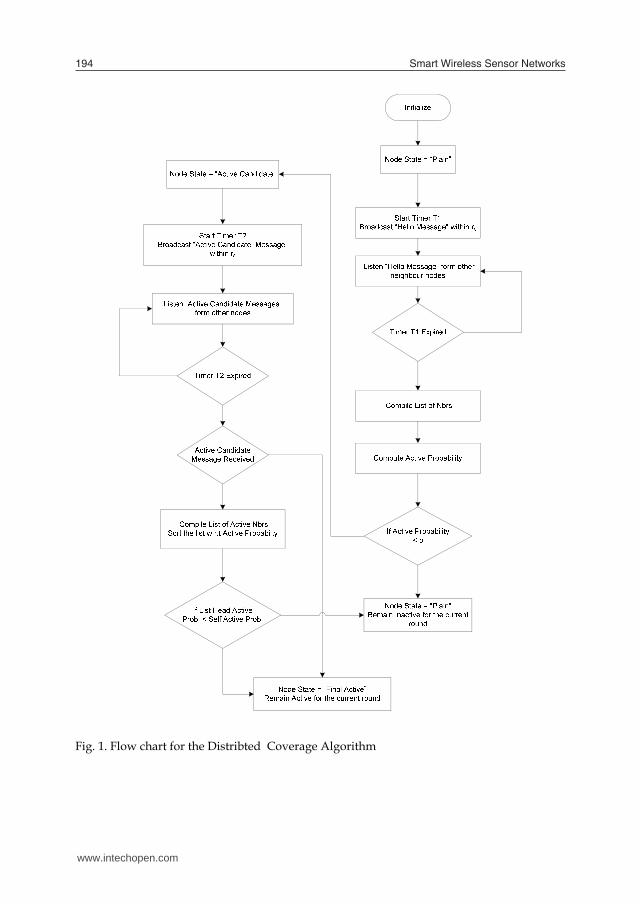
4. Distributed Coverage Algorithm
This Section provides details of our Distributed Coverage Algorithm. The main objective of this algorithm is to select a set of sensor nodes such that each point of interest in the monitoring region is covered by at least one sensor node. Figure 1 describe the flowchart for DCA and its explanation is articulated in the following paragraph. The algorithm consists of three main procedures. In the first procedure, when sensor nodes boot (immediately after deployment in the monitoring region) the initial network discovery process begins. The intial state of all sensor nodes in taken as ‘Plain Nodes’. At this point sensor nodes broadcast a 'Hello' message using a tansmission radius equal to ��. A timer ‘T1’is started locally inside each sensor node. The timer ‘T1’ ensures that sensor nodes have enough time to complete the neighborhood discovery process by receiving 'Hello' messages from other sensor nodes that are within their communication range. When timer ‘T1’ expires, each node compiles a list of its one-hop neighbors. Each node then calculates a probability (referred to here as ‘Active Probability’) by simply generating a random value between 0 and 1 to become an ‘Active Candidate’. In the next procedure, each node compares its ‘Active Probability’ to a pre-defined value 声. If the computed value of ‘Active Probability’ is less than 声, it changes its status to ‘Active Candidate’ and broadcasts an announcement message to its neighbors within range ��. The announcement message contains the value of its computed probability. Again the timer ‘T2’ is used here to ensure that an ‘Active Candidate’ is able to successfully receive announcement messages from other active candidates in its neighborhood. When the timer expires a list of active candidate messages (ACM) is build using information such as node id and ‘Active Probability’. The ACM is sorted with respect to ‘Active Probability’ in decreasing order. If the entry and the head of ACM has a value lower than the node’s computed probability, the sensor node changes its status to 旺繋��欠健 Active’ and broadcasts a notification message. Any ties are broken in favor of the sensor node with higher node id. In the final procedure, all nodes check if they received ‘Final Active’ message. Any node that did not receive this message changes its status to become ‘Final Active’ for the current round.
www.intechopen.com
Optimizing Coverage in 3D Wireless Sensor Networks 193
1. Communication Range: A sphere based communication ranged is assumed where each active sensor has a communication range of ��. For reliable communication the distance between two active sensor is required to be less than or equal to ��.
2. Sensing Region: The sphere based sensing region �� of a sensor �� located at point � ���� ����������� ��� � �� � ��� is the collection of all points where a target � is reliably detected by sensor ��.
3. Similar to (Liu and Towsley 2004), a Boolean sensing model is used. A sensor �� is only able to detect events of interest within its sensing region �� . Given the sensing radius �� from �� , the output of the Boolean model can be described as;
������� ����� � �� ��� �������� ����� � ��� ��������� (1)
Where ����� denotes the position of the sensor, ���� denotes the location of a target and �������� ����� specifies the Euclidean distance between the target and the sensor. In line with the findings in (Zhang and Hou 2005), we assume that the communication range �� is � � ��. We also assume that sensor nodes are capable of transmitting at various power level.
4. Sensor nodes are randomly dispersed over a three dimensional geographical region following a uniform distribution.
5. All sensor nodes are homogeneous in terms of energy, communication, and processing capabilities.
6. We assume that the sensor nodes are capable of switching between sleep and active modes. Most commercially available platform such as IRSI motes (MEMSIC 2011), TelosB (MEMSIC 2011), TMote Sky support features such as auto suspend, wake, and sleep mode that are used to minimize the sensor node's energy consumption.
7. All sensor nodes are location unaware i.e. they are not equipped with a GPS device. 8. The energy model presented in (Heinzelman, Chandrakasan et al. 2002) is adopted
here. The amount of energy consumed for transmission ��� is of an l-bit message over a distance d is given by;
2
4
. . . for 0. . . for
elect fs crossoverTx
elect mp crossover
l E l d d dE
l E l d d d
(2)
Where electE is the amount of energy consumed in electronics, fs is the energy consumed
in an amplifier when transmitting at a distance shorter than crossoverd , and mp is the
amplifier energy consumed in an amplifier when transmitting at a distance greater than
crossoverd . The energy expended in receiving an l-bit message is given by, electRx lEE (3)
4. Distributed Coverage Algorithm
This Section provides details of our Distributed Coverage Algorithm. The main objective of this algorithm is to select a set of sensor nodes such that each point of interest in the monitoring region is covered by at least one sensor node. Figure 1 describe the flowchart for DCA and its explanation is articulated in the following paragraph. The algorithm consists of three main procedures. In the first procedure, when sensor nodes boot (immediately after deployment in the monitoring region) the initial network discovery process begins. The intial state of all sensor nodes in taken as ‘Plain Nodes’. At this point sensor nodes broadcast a 'Hello' message using a tansmission radius equal to ��. A timer ‘T1’is started locally inside each sensor node. The timer ‘T1’ ensures that sensor nodes have enough time to complete the neighborhood discovery process by receiving 'Hello' messages from other sensor nodes that are within their communication range. When timer ‘T1’ expires, each node compiles a list of its one-hop neighbors. Each node then calculates a probability (referred to here as ‘Active Probability’) by simply generating a random value between 0 and 1 to become an ‘Active Candidate’. In the next procedure, each node compares its ‘Active Probability’ to a pre-defined value 声. If the computed value of ‘Active Probability’ is less than 声, it changes its status to ‘Active Candidate’ and broadcasts an announcement message to its neighbors within range ��. The announcement message contains the value of its computed probability. Again the timer ‘T2’ is used here to ensure that an ‘Active Candidate’ is able to successfully receive announcement messages from other active candidates in its neighborhood. When the timer expires a list of active candidate messages (ACM) is build using information such as node id and ‘Active Probability’. The ACM is sorted with respect to ‘Active Probability’ in decreasing order. If the entry and the head of ACM has a value lower than the node’s computed probability, the sensor node changes its status to 旺繋��欠健 Active’ and broadcasts a notification message. Any ties are broken in favor of the sensor node with higher node id. In the final procedure, all nodes check if they received ‘Final Active’ message. Any node that did not receive this message changes its status to become ‘Final Active’ for the current round.
www.intechopen.com
Smart Wireless Sensor Networks194
Fig. 1. Flow chart for the Distribted Coverage Algorithm
It can be noted that the sensing range plays a vital role in determining the area coverage for any given random deployemnt. In order to estimate the appropriate sensing range values for a given deployemnt region and node density we use the Poisson point process model. Let us assume that sensors are dispersed in A with intensity λ. The number of sensors located in A are given by, N�A� � λ|A| (4) Where |A| represents the volume of three-dimensional region. Let � be a randomly chosen point in the target region. We are interested in finding the probability that there is at least one sensor with �������� �� � �� . Assuming a spherical sensing model, the coverage fraction η is given by the probabiliy that the point lies within at least one sensor’s range: � � ���N�A� � �� � � � ���N�A� � �� (5) The probability in (5) for a given intensity is
� � � � ���.������ (6) Solving equation (6) for λ,
λ � ���� ����������� (7)
Using λ in equation (4) and solving for ��,
�� � � � ��������|�|������� ���� (8)
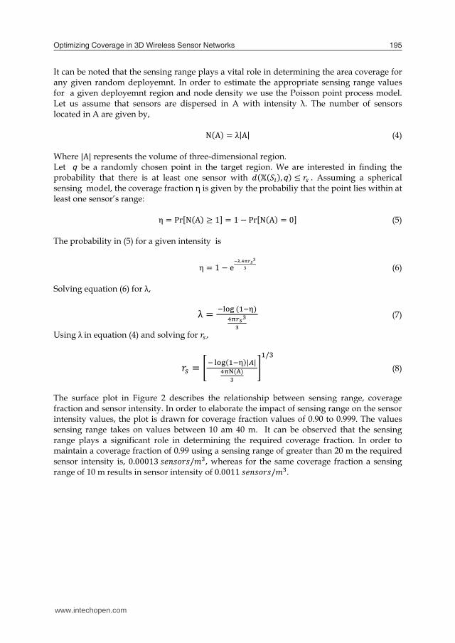
The surface plot in Figure 2 describes the relationship between sensing range, coverage fraction and sensor intensity. In order to elaborate the impact of sensing range on the sensor intensity values, the plot is drawn for coverage fraction values of 0.90 to 0.999. The values sensing range takes on values between 10 am 40 m. It can be observed that the sensing range plays a significant role in determining the required coverage fraction. In order to maintain a coverage fraction of 0.99 using a sensing range of greater than 20 m the required sensor intensity is, �.����� ����������, whereas for the same coverage fraction a sensing range of 10 m results in sensor intensity of �.���� ����������.
www.intechopen.com
Optimizing Coverage in 3D Wireless Sensor Networks 195
Fig. 1. Flow chart for the Distribted Coverage Algorithm
It can be noted that the sensing range plays a vital role in determining the area coverage for any given random deployemnt. In order to estimate the appropriate sensing range values for a given deployemnt region and node density we use the Poisson point process model. Let us assume that sensors are dispersed in A with intensity λ. The number of sensors located in A are given by, N�A� � λ|A| (4) Where |A| represents the volume of three-dimensional region. Let � be a randomly chosen point in the target region. We are interested in finding the probability that there is at least one sensor with �������� �� � �� . Assuming a spherical sensing model, the coverage fraction η is given by the probabiliy that the point lies within at least one sensor’s range: � � ���N�A� � �� � � � ���N�A� � �� (5) The probability in (5) for a given intensity is
� � � � ���.������ (6) Solving equation (6) for λ,
λ � ���� ����������� (7)
Using λ in equation (4) and solving for ��,
�� � � � ��������|�|������� ���� (8)
The surface plot in Figure 2 describes the relationship between sensing range, coverage fraction and sensor intensity. In order to elaborate the impact of sensing range on the sensor intensity values, the plot is drawn for coverage fraction values of 0.90 to 0.999. The values sensing range takes on values between 10 am 40 m. It can be observed that the sensing range plays a significant role in determining the required coverage fraction. In order to maintain a coverage fraction of 0.99 using a sensing range of greater than 20 m the required sensor intensity is, �.����� ����������, whereas for the same coverage fraction a sensing range of 10 m results in sensor intensity of �.���� ����������.
www.intechopen.com
Smart Wireless Sensor Networks196
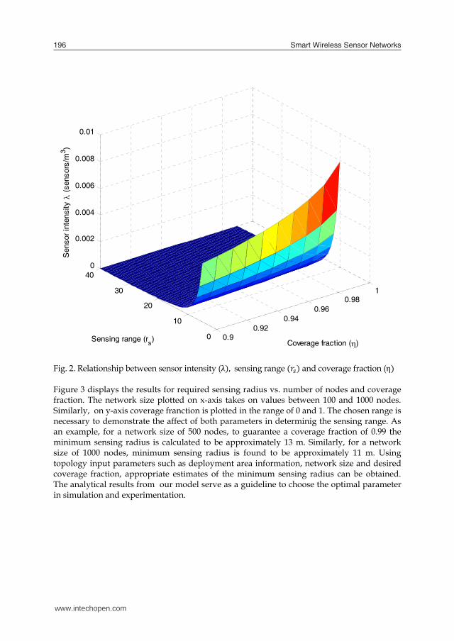
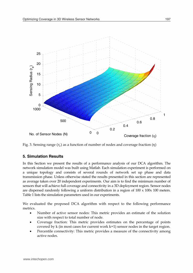
Fig. 2. Relationship between sensor intensity (� sensing range ���� and coverage fraction (�� Figure 3 displays the results for required sensing radius vs. number of nodes and coverage fraction. The network size plotted on x-axis takes on values between 100 and 1000 nodes. Similarly, on y-axis coverage franction is plotted in the range of 0 and 1. The chosen range is necessary to demonstrate the affect of both parameters in determinig the sensing range. As an example, for a network size of 500 nodes, to guarantee a coverage fraction of 0.99 the minimum sensing radius is calculated to be approximately 13 m. Similarly, for a network size of 1000 nodes, minimum sensing radius is found to be approximately 11 m. Using topology input parameters such as deployment area information, network size and desired coverage fraction, appropriate estimates of the minimum sensing radius can be obtained. The analytical results from our model serve as a guideline to choose the optimal parameter in simulation and experimentation.
0.90.92
0.940.96
0.981
0
10
20
30
400
0.002
0.004
0.006
0.008
0.01
Coverage fraction ()Sensing range (rs)
Sen
sor i
nten
sity
(se
nsor
s/m
3 )
Fig. 3. Sensing range ���� as a function of number of nodes and coverage fraction (��
5. Simulation Results
In this Section we present the results of a performance analysis of our DCA algorithm. The network simulation model was built using Matlab. Each simulation experiment is performed on a unique topology and consists of several rounds of network set up phase and data transmission phase. Unless otherwise stated the results presented in this section are represented as average taken over 20 independent experiments. Our aim is to find the minimum number of sensors that will achieve full coverage and connectivity in a 3D deployment region. Sensor nodes are dispersed randomly following a uniform distribution in a region of 100 x 100x 100 meters. Table 1 lists the simulation parameters used in our experiments. We evaluated the proposed DCA algorithm with respect to the following performance metrics.
Number of active sensor nodes: This metric provides an estimate of the solution size with respect to total number of node.
Coverage fraction: This metric provides estimates on the percentage of points covered by k (in most cases for current work k=1) sensor nodes in the target region.
Percentile connectivity: This metric provides a measure of the connectivity among active nodes.
00.2
0.40.6
0.81
0
500
10000
5
10
15
20
25
Coverage fraction ()No. of Sensor Nodes (N)
Sen
sing
Rad
ius
(rs)
www.intechopen.com
Optimizing Coverage in 3D Wireless Sensor Networks 197
Fig. 2. Relationship between sensor intensity (� sensing range ���� and coverage fraction (�� Figure 3 displays the results for required sensing radius vs. number of nodes and coverage fraction. The network size plotted on x-axis takes on values between 100 and 1000 nodes. Similarly, on y-axis coverage franction is plotted in the range of 0 and 1. The chosen range is necessary to demonstrate the affect of both parameters in determinig the sensing range. As an example, for a network size of 500 nodes, to guarantee a coverage fraction of 0.99 the minimum sensing radius is calculated to be approximately 13 m. Similarly, for a network size of 1000 nodes, minimum sensing radius is found to be approximately 11 m. Using topology input parameters such as deployment area information, network size and desired coverage fraction, appropriate estimates of the minimum sensing radius can be obtained. The analytical results from our model serve as a guideline to choose the optimal parameter in simulation and experimentation.
0.90.92
0.940.96
0.981
0
10
20
30
400
0.002
0.004
0.006
0.008
0.01
Coverage fraction ()Sensing range (rs)
Sen
sor i
nten
sity
(se
nsor
s/m
3 )
Fig. 3. Sensing range ���� as a function of number of nodes and coverage fraction (��
5. Simulation Results
In this Section we present the results of a performance analysis of our DCA algorithm. The network simulation model was built using Matlab. Each simulation experiment is performed on a unique topology and consists of several rounds of network set up phase and data transmission phase. Unless otherwise stated the results presented in this section are represented as average taken over 20 independent experiments. Our aim is to find the minimum number of sensors that will achieve full coverage and connectivity in a 3D deployment region. Sensor nodes are dispersed randomly following a uniform distribution in a region of 100 x 100x 100 meters. Table 1 lists the simulation parameters used in our experiments. We evaluated the proposed DCA algorithm with respect to the following performance metrics.
Number of active sensor nodes: This metric provides an estimate of the solution size with respect to total number of node.
Coverage fraction: This metric provides estimates on the percentage of points covered by k (in most cases for current work k=1) sensor nodes in the target region.
Percentile connectivity: This metric provides a measure of the connectivity among active nodes.
00.2
0.40.6
0.81
0
500
10000
5
10
15
20
25
Coverage fraction ()No. of Sensor Nodes (N)
Sen
sing
Rad
ius
(rs)
www.intechopen.com
Smart Wireless Sensor Networks198
Network Size 200 – 600 nodes
Area Dimensions 100 x 100 x 100 m
Sensing Range (��� 15 – 25 m
Communication Range (��� 2* (���
Probabililty p 0.15
Initial Energy 0.5 J
Message Size 25 Bytes
.ElectE - Energy spent in electronics 50 n J /bit
fs - Constant for free space propagation 10 p J/bit/m2
mp - Constant for multi-path propagation .0013 p J/bit/m4
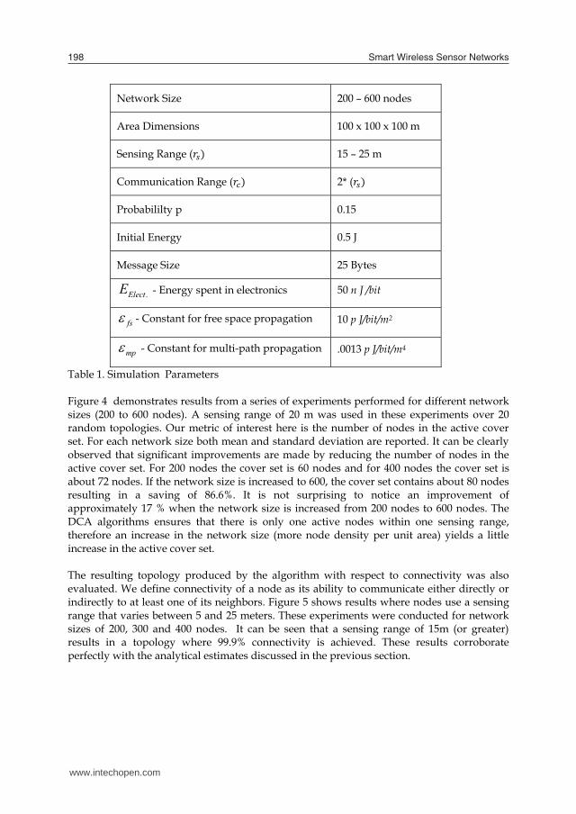
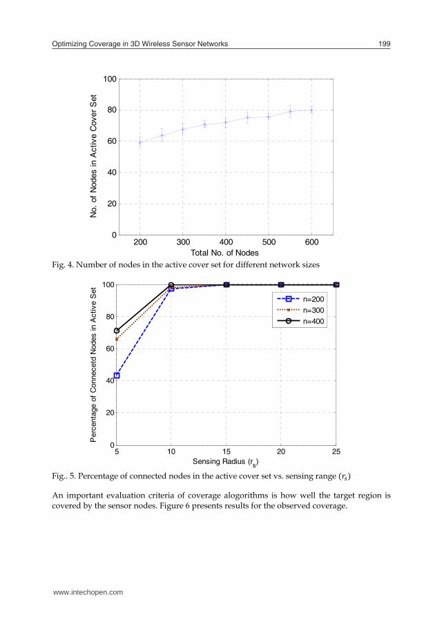
Table 1. Simulation Parameters Figure 4 demonstrates results from a series of experiments performed for different network sizes (200 to 600 nodes). A sensing range of 20 m was used in these experiments over 20 random topologies. Our metric of interest here is the number of nodes in the active cover set. For each network size both mean and standard deviation are reported. It can be clearly observed that significant improvements are made by reducing the number of nodes in the active cover set. For 200 nodes the cover set is 60 nodes and for 400 nodes the cover set is about 72 nodes. If the network size is increased to 600, the cover set contains about 80 nodes resulting in a saving of 86.6%. It is not surprising to notice an improvement of approximately 17 % when the network size is increased from 200 nodes to 600 nodes. The DCA algorithms ensures that there is only one active nodes within one sensing range, therefore an increase in the network size (more node density per unit area) yields a little increase in the active cover set. The resulting topology produced by the algorithm with respect to connectivity was also evaluated. We define connectivity of a node as its ability to communicate either directly or indirectly to at least one of its neighbors. Figure 5 shows results where nodes use a sensing range that varies between 5 and 25 meters. These experiments were conducted for network sizes of 200, 300 and 400 nodes. It can be seen that a sensing range of 15m (or greater) results in a topology where 99.9% connectivity is achieved. These results corroborate perfectly with the analytical estimates discussed in the previous section.
Fig. 4. Number of nodes in the active cover set for different network sizes
Fig.. 5. Percentage of connected nodes in the active cover set vs. sensing range ����
An important evaluation criteria of coverage alogorithms is how well the target region is covered by the sensor nodes. Figure 6 presents results for the observed coverage.
200 300 400 500 6000
20
40
60
80
100
Total No. of Nodes
No.
of
Nod
es in
Act
ive
Cov
er S
et
5 10 15 20 250
20
40
60
80
100
Sensing Radius (rs)
Per
cent
age
of C
onne
cetd
Nod
es in
Act
ive
Set
n=200n=300n=400
www.intechopen.com
Optimizing Coverage in 3D Wireless Sensor Networks 199
Network Size 200 – 600 nodes
Area Dimensions 100 x 100 x 100 m
Sensing Range (��� 15 – 25 m
Communication Range (��� 2* (���
Probabililty p 0.15
Initial Energy 0.5 J
Message Size 25 Bytes
.ElectE - Energy spent in electronics 50 n J /bit
fs - Constant for free space propagation 10 p J/bit/m2
mp - Constant for multi-path propagation .0013 p J/bit/m4
Table 1. Simulation Parameters Figure 4 demonstrates results from a series of experiments performed for different network sizes (200 to 600 nodes). A sensing range of 20 m was used in these experiments over 20 random topologies. Our metric of interest here is the number of nodes in the active cover set. For each network size both mean and standard deviation are reported. It can be clearly observed that significant improvements are made by reducing the number of nodes in the active cover set. For 200 nodes the cover set is 60 nodes and for 400 nodes the cover set is about 72 nodes. If the network size is increased to 600, the cover set contains about 80 nodes resulting in a saving of 86.6%. It is not surprising to notice an improvement of approximately 17 % when the network size is increased from 200 nodes to 600 nodes. The DCA algorithms ensures that there is only one active nodes within one sensing range, therefore an increase in the network size (more node density per unit area) yields a little increase in the active cover set. The resulting topology produced by the algorithm with respect to connectivity was also evaluated. We define connectivity of a node as its ability to communicate either directly or indirectly to at least one of its neighbors. Figure 5 shows results where nodes use a sensing range that varies between 5 and 25 meters. These experiments were conducted for network sizes of 200, 300 and 400 nodes. It can be seen that a sensing range of 15m (or greater) results in a topology where 99.9% connectivity is achieved. These results corroborate perfectly with the analytical estimates discussed in the previous section.
Fig. 4. Number of nodes in the active cover set for different network sizes
Fig.. 5. Percentage of connected nodes in the active cover set vs. sensing range ����
An important evaluation criteria of coverage alogorithms is how well the target region is covered by the sensor nodes. Figure 6 presents results for the observed coverage.
200 300 400 500 6000
20
40
60
80
100
Total No. of Nodes
No.
of
Nod
es in
Act
ive
Cov
er S
et
5 10 15 20 250
20
40
60
80
100
Sensing Radius (rs)
Per
cent
age
of C
onne
cetd
Nod
es in
Act
ive
Set
n=200n=300n=400
www.intechopen.com
Smart Wireless Sensor Networks200
(a) Network Size=200
(b) Network Size=300
(c) Network Size=400
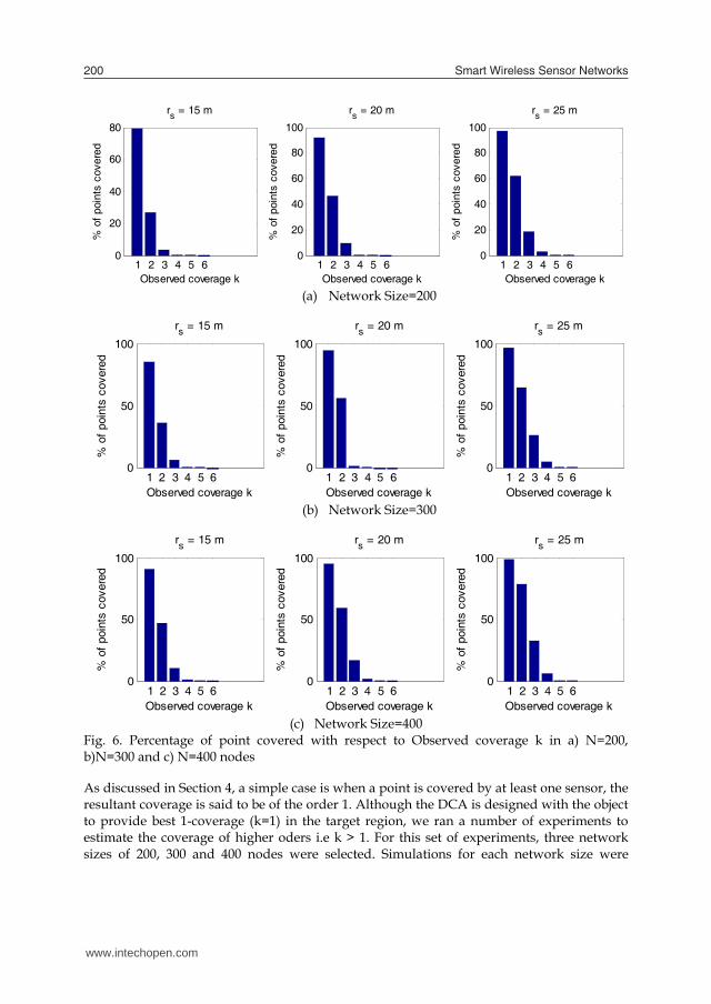
Fig. 6. Percentage of point covered with respect to Observed coverage k in a) N=200, b)N=300 and c) N=400 nodes As discussed in Section 4, a simple case is when a point is covered by at least one sensor, the resultant coverage is said to be of the order 1. Although the DCA is designed with the object to provide best 1-coverage (k=1) in the target region, we ran a number of experiments to estimate the coverage of higher oders i.e k > 1. For this set of experiments, three network sizes of 200, 300 and 400 nodes were selected. Simulations for each network size were
1 2 3 4 5 60
20
40
60
80
Observed coverage k
% o
f po
ints
cov
ered
rs = 15 m
1 2 3 4 5 60
20
40
60
80
100
Observed coverage k%
of
poin
ts c
over
ed
rs = 20 m
1 2 3 4 5 60
20
40
60
80
100
Observed coverage k
% o
f po
ints
cov
ered
rs = 25 m
1 2 3 4 5 60
50
100
Observed coverage k
% o
f po
ints
cov
ered
rs = 15 m
1 2 3 4 5 60
50
100
Observed coverage k
% o
f po
ints
cov
ered
rs = 20 m
1 2 3 4 5 60
50
100
Observed coverage k
% o
f po
ints
cov
ered
rs = 25 m
1 2 3 4 5 60
50
100
Observed coverage k
% o
f po
ints
cov
ered
rs = 15 m
1 2 3 4 5 60
50
100
Observed coverage k
% o
f po
ints
cov
ered
rs = 20 m
1 2 3 4 5 60
50
100
Observed coverage k
% o
f po
ints
cov
ered
rs = 25 m
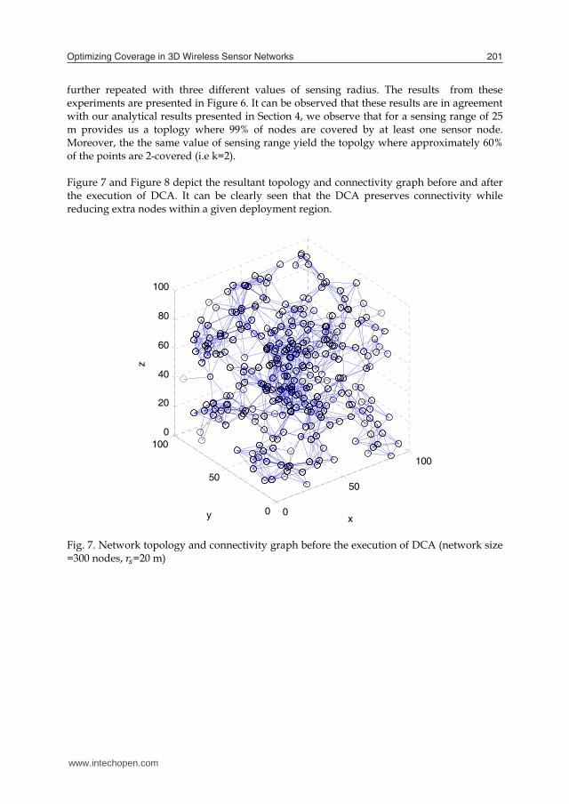
further repeated with three different values of sensing radius. The results from these experiments are presented in Figure 6. It can be observed that these results are in agreement with our analytical results presented in Section 4, we observe that for a sensing range of 25 m provides us a toplogy where 99% of nodes are covered by at least one sensor node. Moreover, the the same value of sensing range yield the topolgy where approximately 60% of the points are 2-covered (i.e k=2). Figure 7 and Figure 8 depict the resultant topology and connectivity graph before and after the execution of DCA. It can be clearly seen that the DCA preserves connectivity while reducing extra nodes within a given deployment region.
Fig. 7. Network topology and connectivity graph before the execution of DCA (network size =300 nodes, ��=20 m)
0
50
100
0
50
1000
20
40
60
80
100
xy
z
www.intechopen.com
Optimizing Coverage in 3D Wireless Sensor Networks 201
(a) Network Size=200
(b) Network Size=300
(c) Network Size=400
Fig. 6. Percentage of point covered with respect to Observed coverage k in a) N=200, b)N=300 and c) N=400 nodes As discussed in Section 4, a simple case is when a point is covered by at least one sensor, the resultant coverage is said to be of the order 1. Although the DCA is designed with the object to provide best 1-coverage (k=1) in the target region, we ran a number of experiments to estimate the coverage of higher oders i.e k > 1. For this set of experiments, three network sizes of 200, 300 and 400 nodes were selected. Simulations for each network size were
1 2 3 4 5 60
20
40
60
80
Observed coverage k
% o
f po
ints
cov
ered
rs = 15 m
1 2 3 4 5 60
20
40
60
80
100
Observed coverage k
% o
f po
ints
cov
ered
rs = 20 m
1 2 3 4 5 60
20
40
60
80
100
Observed coverage k
% o
f po
ints
cov
ered
rs = 25 m
1 2 3 4 5 60
50
100
Observed coverage k
% o
f po
ints
cov
ered
rs = 15 m
1 2 3 4 5 60
50
100
Observed coverage k
% o
f po
ints
cov
ered
rs = 20 m
1 2 3 4 5 60
50
100
Observed coverage k
% o
f po
ints
cov
ered
rs = 25 m
1 2 3 4 5 60
50
100
Observed coverage k
% o
f po
ints
cov
ered
rs = 15 m
1 2 3 4 5 60
50
100
Observed coverage k
% o
f po
ints
cov
ered
rs = 20 m
1 2 3 4 5 60
50
100
Observed coverage k
% o
f po
ints
cov
ered
rs = 25 m
further repeated with three different values of sensing radius. The results from these experiments are presented in Figure 6. It can be observed that these results are in agreement with our analytical results presented in Section 4, we observe that for a sensing range of 25 m provides us a toplogy where 99% of nodes are covered by at least one sensor node. Moreover, the the same value of sensing range yield the topolgy where approximately 60% of the points are 2-covered (i.e k=2). Figure 7 and Figure 8 depict the resultant topology and connectivity graph before and after the execution of DCA. It can be clearly seen that the DCA preserves connectivity while reducing extra nodes within a given deployment region.
Fig. 7. Network topology and connectivity graph before the execution of DCA (network size =300 nodes, ��=20 m)
0
50
100
0
50
1000
20
40
60
80
100
xy
z
www.intechopen.com
Smart Wireless Sensor Networks202
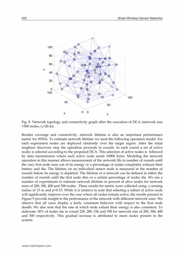
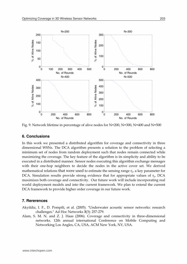
Fig. 8. Network topology and connectivity graph after the execution of DCA (network size =300 nodes, ��=20 m) Besides coverage and conenctivity, network lifetime is also an important performance metric for WSNs. To estimate network lifetime we used the following operation model. For each experiment nodes are deployed randomly over the target region. After the intial neighnor discovery step the operation proceeds in rounds. In each round a set of active nodes is selected according to the proposed DCA. This selection of active nodes is followed by data transmission where each active node sends 10000 bytes. Modeling the network operation in this manner allows measurement of the network life in number of rounds until the very first node runs out of its energy or a percentage of nodes completely exhaust their battery and die. The lifetime on an individual sensor node is measured in the number of rounds before its energy is depleted. The lifetime of a network can be defined in either the number of rounds until the first node dies or a certain percentage of nodes die. We ran a number of experiments to estimate network lifetime in percent of alive nodes for network sizes of 200, 300, 400 and 500 nodes. These results for metric were collected using a sensing radius of 15 m and p=0.15. While it is intutive to note that selecting a subset of active node will significantly improve over the case where all nodes remain active, the results present in Figure 9 provide insight to the perfromance of the network with different network sizes. We observe that all cases display a fairly consistent behavior with respect to the first node deatth. We also note that the rate at which node exhust their energy is also consistent. To elaborate, 50% of nodes die in round 238, 280, 336 and 390 for network size of 200, 300, 400 and 500 respectively. This gradual increase is attributed to more nodes present in the system.
0
50
100
0
50
1000
20
40
60
80
100
xy
z
Fig. 9. Network lifetime in percentage of alive nodes for N=200, N=300, N=400 and N=500
6. Conclusions
In this work we presented a distributed algorithm for coverage and connectivity in three dimensional WSNs. The DCA algorithm presents a solution to the problem of selecting a minimum set of nodes from random deployment such that nodes remain connected while maximizing the coverage. The key feature of the algorithm is its simplicity and ability to be executed in a distributed manner. Sensor nodes executing this algorithm exchange messages with their one-hop neighbors to decide the nodes in the active cover set. We derived mathematical relations that were used to estimate the sensing range ��, a key parameter for DCA. Simulation results provide strong evidence that for appropriate values of ��, DCA maximizes both coverage and connectivity. Our future work will include incorporating real world deployment models and into the current framework. We plan to extend the current DCA framework to provide higher order coverage in our future work.
7. Rererences
Akyildiz, I. F., D. Pompili, et al. (2005). "Underwater acoustic sensor networks: research challenges." Ad Hoc Networks 3(3): 257-279.
Alam, S. M. N. and Z. J. Haas (2006). Coverage and connectivity in three-dimensional networks. 12th annual international Conference on Mobile Computing and Networking Los Angles, CA, USA, ACM New York, NY, USA.
0 100 200 300 400 5000
50
100
150
200
No. of Rounds
% o
f A
live
Nod
es
N=200
0 200 400 600 8000
100
200
300
No. of Rounds
% o
f A
live
Nod
es
N=300
0 200 400 600 8000
100
200
300
400
No. of Rounds
% o
f A
live
Nod
es
N=400
0 200 400 600 8000
100
200
300
400
500N=500
No. of Rounds
% o
f A
live
Nod
es
www.intechopen.com
Optimizing Coverage in 3D Wireless Sensor Networks 203
Fig. 8. Network topology and connectivity graph after the execution of DCA (network size =300 nodes, ��=20 m) Besides coverage and conenctivity, network lifetime is also an important performance metric for WSNs. To estimate network lifetime we used the following operation model. For each experiment nodes are deployed randomly over the target region. After the intial neighnor discovery step the operation proceeds in rounds. In each round a set of active nodes is selected according to the proposed DCA. This selection of active nodes is followed by data transmission where each active node sends 10000 bytes. Modeling the network operation in this manner allows measurement of the network life in number of rounds until the very first node runs out of its energy or a percentage of nodes completely exhaust their battery and die. The lifetime on an individual sensor node is measured in the number of rounds before its energy is depleted. The lifetime of a network can be defined in either the number of rounds until the first node dies or a certain percentage of nodes die. We ran a number of experiments to estimate network lifetime in percent of alive nodes for network sizes of 200, 300, 400 and 500 nodes. These results for metric were collected using a sensing radius of 15 m and p=0.15. While it is intutive to note that selecting a subset of active node will significantly improve over the case where all nodes remain active, the results present in Figure 9 provide insight to the perfromance of the network with different network sizes. We observe that all cases display a fairly consistent behavior with respect to the first node deatth. We also note that the rate at which node exhust their energy is also consistent. To elaborate, 50% of nodes die in round 238, 280, 336 and 390 for network size of 200, 300, 400 and 500 respectively. This gradual increase is attributed to more nodes present in the system.
0
50
100
0
50
1000
20
40
60
80
100
xy
z
Fig. 9. Network lifetime in percentage of alive nodes for N=200, N=300, N=400 and N=500
6. Conclusions
In this work we presented a distributed algorithm for coverage and connectivity in three dimensional WSNs. The DCA algorithm presents a solution to the problem of selecting a minimum set of nodes from random deployment such that nodes remain connected while maximizing the coverage. The key feature of the algorithm is its simplicity and ability to be executed in a distributed manner. Sensor nodes executing this algorithm exchange messages with their one-hop neighbors to decide the nodes in the active cover set. We derived mathematical relations that were used to estimate the sensing range ��, a key parameter for DCA. Simulation results provide strong evidence that for appropriate values of ��, DCA maximizes both coverage and connectivity. Our future work will include incorporating real world deployment models and into the current framework. We plan to extend the current DCA framework to provide higher order coverage in our future work.
7. Rererences
Akyildiz, I. F., D. Pompili, et al. (2005). "Underwater acoustic sensor networks: research challenges." Ad Hoc Networks 3(3): 257-279.
Alam, S. M. N. and Z. J. Haas (2006). Coverage and connectivity in three-dimensional networks. 12th annual international Conference on Mobile Computing and Networking Los Angles, CA, USA, ACM New York, NY, USA.
0 100 200 300 400 5000
50
100
150
200
No. of Rounds
% o
f A
live
Nod
esN=200
0 200 400 600 8000
100
200
300
No. of Rounds
% o
f A
live
Nod
es
N=300
0 200 400 600 8000
100
200
300
400
No. of Rounds
% o
f A
live
Nod
es
N=400
0 200 400 600 8000
100
200
300
400
500N=500
No. of Rounds
% o
f A
live
Nod
es
www.intechopen.com
Smart Wireless Sensor Networks204
Andersen, T. and S. Tirthapura (2009). Wireless sensor deployment for 3D coverage with constraints. Sixth International Conference on Networked Sensing Systems (INSS).
Bai, X., S. Kumar, et al. (2006). Deploying wireless sensors to achieve both coverage and connectivity. ACM Mobihoc, ACM New York, NY, USA.
Cardei, M. and J. Wu (2006). "Energy-efficient coverage problems in wireless ad-hoc sensor networks." Computer communications 29(4): 413-420.
Cayirci, E., H. Tezcan, et al. (2006). "Wireless sensor networks for underwater survelliance systems." Ad Hoc Networks 4(4): 431-446.
Chen, F., P. Jiang, et al. (2008). "Probability-Based Coverage Algorithm for 3D Wireless Sensor Networks." Advanced Intelligent Computing Theories and Applications. With Aspects of Contemporary Intelligent Computing Techniques, Communications in Computer and Information Science 15.
Heinzelman, W. B., A. P. Chandrakasan, et al. (2002). "An application-specific protocol architecture for wireless microsensor networks." IEEE Transactions on wireless communications 1(4): 660-670.
Huang, C. F., Y. C. Tseng, et al. (2004). The coverage problem in three-dimensional wireless sensor networks. IEEE Global Telecommunications Conference.
I. F. Akyildiz, W. Su, et al. (2002). " A Survey on Sensor Networks." IEEE Communications Magazine 40(8): 102-114.
Iyengar, R., K. Kar, et al. (2005). Low-coordination topologies for redundancy in sensor networks, ACM.
Kim, S., S. Pakzad, et al. (2006). "Wireless sensor networks for structural health monitoring." Proceedings of the 4th international conference on Embedded networked sensor systems: 427-428.
Liu, B. and D. Towsley (2004). A study of the coverage of large-scale sensor networks. IEEE International Conference on Mobile Ad-hoc and Sensor Systems (MASS)
Lynch, J. P. and K. J. Loh (2006). "A summary review of wireless sensors and sensor networks for structural health monitoring." Shock and Vibration Digest 38(2): 91-130.
Mainwaring, A., D. Culler, et al. (2002). Wireless sensor networks for habitat monitoring, ACM. MEMSIC. (2011). "IRIS Mote Data Sheet." from http://www.memsic.com/products/wireless-sensor-networks/wireless-
modules.html. MEMSIC. (2011). "TelosB Data Sheet." from http://www.memsic.com/products/wireless-
sensor-networks/wireless-modules.html. Poduri, S., S. Pattem, et al. (2006). Sensor network configuration and the curse of
dimensionality. The Third IEEE Workshop on Embedded Networked Sensors (EmNets), Cambridge, MA, USA.
Szewczyk, R., E. Osterweil, et al. (2004). "Habitat monitoring with sensor networks." Communications of the ACM 47(6): 34-40.
Xing, G., X. Wang, et al. (2005). "Integrated coverage and connectivity configuration for energy conservation in sensor networks." ACM Transactions on Sensor Networks (TOSN) 1(1): 36-72.
Yang, S., F. Dai, et al. (2006). "On connected multiple point coverage in wireless sensor networks." International Journal of Wireless Information Networks 13(4): 289-301.
Zhang, H. and J. C. Hou (2005). "Maintaining sensing coverage and connectivity in large sensor networks." Ad Hoc & Sensor Wireless Networks 1(1-2): 89-124.
www.intechopen.com
Smart Wireless Sensor NetworksEdited by Yen Kheng Tan
ISBN 978-953-307-261-6Hard cover, 418 pagesPublisher InTechPublished online 14, December, 2010Published in print edition December, 2010
InTech EuropeUniversity Campus STeP Ri Slavka Krautzeka 83/A 51000 Rijeka, Croatia Phone: +385 (51) 770 447
InTech ChinaUnit 405, Office Block, Hotel Equatorial Shanghai No.65, Yan An Road (West), Shanghai, 200040, China
Phone: +86-21-62489820 Fax: +86-21-62489821
The recent development of communication and sensor technology results in the growth of a new attractive andchallenging area – wireless sensor networks (WSNs). A wireless sensor network which consists of a largenumber of sensor nodes is deployed in environmental fields to serve various applications. Facilitated with theability of wireless communication and intelligent computation, these nodes become smart sensors which do notonly perceive ambient physical parameters but also be able to process information, cooperate with each otherand self-organize into the network. These new features assist the sensor nodes as well as the network tooperate more efficiently in terms of both data acquisition and energy consumption. Special purposes of theapplications require design and operation of WSNs different from conventional networks such as the internet.The network design must take into account of the objectives of specific applications. The nature of deployedenvironment must be considered. The limited of sensor nodes’ resources such as memory, computationalability, communication bandwidth and energy source are the challenges in network design. A smart wirelesssensor network must be able to deal with these constraints as well as to guarantee the connectivity, coverage,reliability and security of network’s operation for a maximized lifetime. This book discusses various aspectsof designing such smart wireless sensor networks. Main topics includes: design methodologies, networkprotocols and algorithms, quality of service management, coverage optimization, time synchronization andsecurity techniques for sensor networks.
How to referenceIn order to correctly reference this scholarly work, feel free to copy and paste the following:
Nauman Aslam (2010). Optimizing Coverage in 3D Wireless Sensor Networks, Smart Wireless SensorNetworks, Yen Kheng Tan (Ed.), ISBN: 978-953-307-261-6, InTech, Available from:http://www.intechopen.com/books/smart-wireless-sensor-networks/optimizing-coverage-in-3d-wireless-sensor-networks
www.intechopen.com

Fax: +385 (51) 686 166www.intechopen.com
Fax: +86-21-62489821

© 2010 The Author(s). Licensee IntechOpen. This chapter is distributedunder the terms of the Creative Commons Attribution-NonCommercial-ShareAlike-3.0 License, which permits use, distribution and reproduction fornon-commercial purposes, provided the original is properly cited andderivative works building on this content are distributed under the samelicense.