Embed Size (px)
Citation preview

Navigation and Localisation of Autonomous Vehicles
Matthew Ricci
SID: 9930385
Australian Centre of Field Robotics,
Department of Mechanical Mechatronic and Aeronautical engineering,
University of Sydney
Supervisor: Dr. Eduardo Nebot
November 2002
A thesis submitted in partial fulfillment of a bachelor of mechanical (Mechatronics) engineering

Acknowledgements
I would first of all like to thanks all those in the ACFR who helped me during the course
of this thesis, especially to Juan Nieto who was always willing to take time out to explain
things to me even when he might have been busy.
I also want to thank my fiancée Leah for her support during this time, I know it has been
tough not being able to see me much, but I thank you for being supportive.
I would also like to thank Benedikt for being a great work partner, without him, working
on this thesis would have been a lot more tedious. Thanks also to Jiri and Kenny for
gracing us with your presence and providing me with someone to beat in AFL slime.
Finally I would like to thank Conrad for his input in this thesis
Matthew Ricci -i-

Statement of Student Contribution
�� I wrote a C version of the encoder/GPS kalman filter
�� I tuned this filter offline to handle various types of GPS data
�� I implemented a real time version of the filter in hyperkernal and wrote a simple
GUI to plot vehicle paths in real time
�� I conducted tests to ensure that the filter worked reliably in real time
�� I implemented a laser based dead reckoning routine based on matching
consecutive features from laser scans in C
�� I researched the maximal common subgraph algorithm for data association and
implemented this on a sample laser data
The above is an accurate statement of the students contribution.
Dr. Eduardo Nebot
Thesis Supervisor
Matthew Ricci -ii-
Abstract
This thesis aims to develop a reliable, robust and accurate navigation filter for use on an
autonomous land vehicle. The filter developed was based on a kalman filter
implementation fusing data from model-based predictions using velocity and steering
information and the absolute position information provided by the GPS. The filter was
tuned to be able to deal with multipath efficiently and still provide accurate position
estimates. An offline simulation was developed and this was then ported to a real time
implementation using the Hyperkernal real time operating system. Extensive testing on
filter performance was conducted to ensure that the filter performed adequately under
most conditions.
An investigation into whether consecutive laser scans could be used to localize the
vehicle. A robust data association technique was developed based on a maximal subgraph
between two graphs. Techniques for extracting features from raw laser data were also
investigated and this data used to calculate pose change between consecutive scans.
Matthew Ricci -iii-

Table of Contents
Acknowledgements ............................................................................................................ i
Statement of Student Contribution................................................................................. ii
Abstract ............................................................................................................................ iii
Table of Figures ............................................................................................................. viii
Chapter 1: Introduction .............................................................................................. 1
1.1 Background to the High Speed Vehicle (HSV) project....................................... 1
1.1.1 Test Vehicle................................................................................................ 1
1.1.2 Hyperkernal ................................................................................................ 4
1.1.3 Past and Current Work ............................................................................... 6
1.2 Goals of this Thesis ............................................................................................ 6
1.3 Thesis Outline..................................................................................................... 7
Chapter 2: Statistical Estimation................................................................................ 8
2.1 Introduction ........................................................................................................ 8
2.2 Kalman Filter ..................................................................................................... 9
2.3 Extended Kalman Filter ................................................................................... 12
2.4 Filter Accuracy and Fault Detection................................................................ 13
Chapter 3: Coordinate Frames................................................................................. 15
3.1 Earth Centred Earth Frames............................................................................ 15
3.1.1 ECEF Rectangular coordinates................................................................. 15
3.1.2 ECEF Geodetic coordinates ..................................................................... 16
3.2 Local Navigation frame.................................................................................... 16
3.3 Body Frame ...................................................................................................... 17
Matthew Ricci -iv-

Chapter 4: Model Based Dead Reckoning............................................................... 18
4.1 Vehicle Model ................................................................................................... 18
4.2 Kalman Filter Implementation ......................................................................... 20
4.2.1 Predictions ................................................................................................ 21
4.2.2 Update....................................................................................................... 22
4.3 Multipath .......................................................................................................... 24
4.4 Fault Detection................................................................................................. 25
4.5 Filter Tuning..................................................................................................... 25
4.6 Initialisation ..................................................................................................... 30
4.7 Limitations........................................................................................................ 31
4.8 Conclusion........................................................................................................ 31
Chapter 5: Laser Dead Reckoning ........................................................................... 32
5.1 Iterative Closest Point and Variations ............................................................. 32
5.2 Feature Extraction............................................................................................ 35
5.2.1 Clustering ................................................................................................. 35
5.2.2 Classification of Objects........................................................................... 37
5.2.3 Line Detection .......................................................................................... 38
5.2.3.1 Line representation ............................................................................... 38
5.2.3.2 Least squares regression parameters .................................................... 39
5.2.3.3 Coefficient of Determination Testing................................................... 43
5.2.3.4 Variance Testing................................................................................... 45
5.2.3.5 Corner Method...................................................................................... 46
5.2.3.6 Summary of Line fitting ....................................................................... 47
5.2.4 Circle Extraction....................................................................................... 48
5.3 Data Association .............................................................................................. 51
5.3.1 Graph Theoretic Approach ....................................................................... 52
5.3.1.1 Feature Graph Generation .................................................................... 52
5.3.1.2 Correspondence Graph Generation ...................................................... 53
5.3.1.3 Maximum Clique.................................................................................. 56
Matthew Ricci -v- 5.3.1.4 Effectiveness of the Graph theoretic approach..................................... 57
5.4 Pose Change Calculation ................................................................................. 60
5.4.1 Circle only Transformation ...................................................................... 60
5.4.2 Line only Transformation......................................................................... 61
5.4.3 Line and Circle Transformation ............................................................... 62
5.4.4 Coordinate Transform .............................................................................. 63
5.5 Conclusion........................................................................................................ 64
Chapter 6: Software Implementation ...................................................................... 65
6.1 Model Based Dead Reckoning.......................................................................... 65
6.1.1 Matrix Functions ...................................................................................... 66
6.1.2 Real Time Implementation ....................................................................... 66
6.1.3 Graphic User Interface ............................................................................. 68
6.2 Laser Based dead reckoning ............................................................................ 69
6.2.1 Graph Representation ............................................................................... 69
Chapter 7: Results...................................................................................................... 72
7.1 Model Based Dead Reckoning.......................................................................... 73
7.1.1 Accuracy of the Model ............................................................................. 73
7.1.2 Offline Filter Performance ....................................................................... 75
7.1.2.1 Accurate GPS ....................................................................................... 75
7.1.2.2 Inaccurate GPS ..................................................................................... 81
7.1.3 Online Results .......................................................................................... 86
7.1.4 Summary................................................................................................... 87
7.2 Laser Dead Reckoning ..................................................................................... 88
7.2.1 Feature Extraction .................................................................................... 88
7.2.1.1 Line Detection ...................................................................................... 88
7.2.1.2 Circle Extraction................................................................................... 92
7.2.2 Data Association....................................................................................... 93
7.2.3 Summary................................................................................................... 97
Chapter 8: Conclusion ............................................................................................... 99
Chapter 9: Bibliography.......................................................................................... 101
Matthew Ricci -vi-

Abbreviations................................................................................................................ 104
Appendix A.................................................................................................................... 105
Appendix B.................................................................................................................... 108
Appendix C.................................................................................................................... 110
Appendix D.................................................................................................................... 112
Matthew Ricci -vii-
Table of Figures
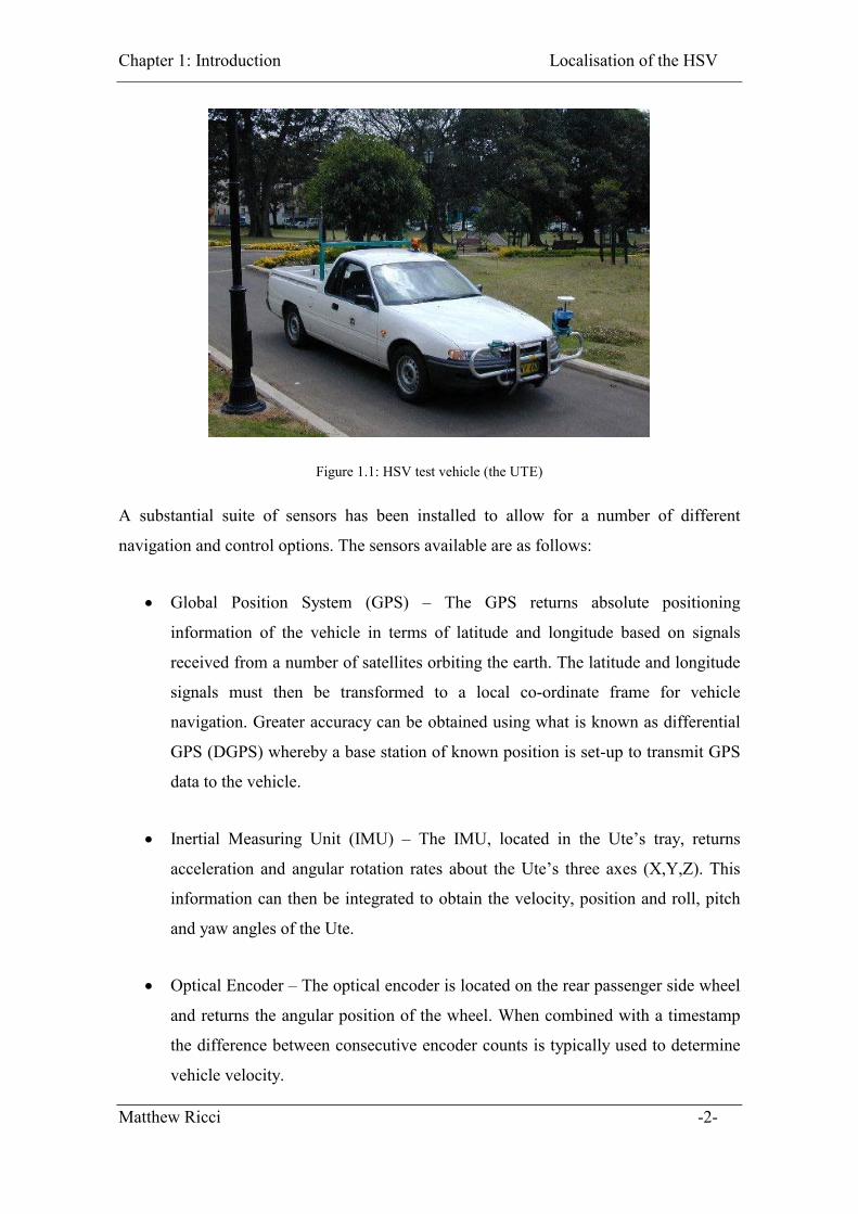
Figure 1.1: HSV test vehicle (the UTE) ............................................................................. 2
Figure 1.2: Steering control motor and clutch.................................................................... 4
Figure 1.3: Hyperkernal shared memory architecture ........................................................ 5
Figure 3.1: ECEF coordinate systems. ECEF rectangular (X,Y,Z) and ECEF geodetic (�
is longitude, � is latitude and h is altitude ................................................................ 16
Figure 3.2: Local NED navigation frame [7] ................................................................... 17
Figure 3.3: Cartesian and polar body frames.................................................................... 17
Figure 4.1: Vehicle model used for dead reckoning......................................................... 19
Figure 4.2: Faulty GPS data taken from the area next to the ACFR building, caused by
the Ute passing under a tree and near a building. ..................................................... 25
Figure 4.3: Low process noise. The blue indicates the filtered position and the red
indicates the observed GPS position. ....................................................................... 26
Figure 4.4: High process noise. The blue indicates the filtered position and the red the
observed GPS position ............................................................................................. 27
Figure 4.5: Low observation noise. Observed GPS data in red and filtered path estimate
in blue. ...................................................................................................................... 28
Figure 4.6: Large observation noise. Estimated path in blue, observations in red. .......... 28
Figure 4.7: Filter never recovering form detection of multipath...................................... 29
Figure 4.8: Incorrect filter tuning failing to recognise multipath effects ......................... 30
Figure 5.1: Shows the ICP method working well when both scans contain the same
features. The blue scan is the first (reference) scan and the red shows the second
scan. The purple represents the second scan moved to the same frame of reference
as the first scan. ........................................................................................................ 34
Figure 5.2: Shows the ICP method breaking down as new features and points are
introduced into the second scan. The blue represents the first scan, the red the
Matthew Ricci -viii-

second and the purple the second scan transformed to be in the same reference
frame as the first scan. .............................................................................................. 35
Figure 5.3: Showing the effects of how some laser pulses fail to return due to the pulse
being lost .................................................................................................................. 36
Figure 5.4: Example of successful clustering. Different clusters are shown in different
colours. Note in the large purple cluster the three points to the right (separated by a
small gap from the rest of the points) are still included in the cluster...................... 37
Figure 5.5: Polar representation of a line ......................................................................... 39
Figure 5.6: Typical values for the coefficient of determination (R2) ............................... 42
Figure 5.7: The variation in points from the line. On the left is the variation in y caused
by a y to x regression and on the right is the variation in x caused by an x to y
regression.................................................................................................................. 43
Figure 5.8: Laser points in a near perfect straight line, demonstrating a coefficient of
correlation of R2 = 0.9995 ........................................................................................ 44
Figure 5.9: Scan of points showing where the R2 tests break down across the middle
section (R2 threshold was set to 0.5 for this test)...................................................... 45
Figure 5.10: Showing the variance method correcting the problems associated with the R2
test............................................................................................................................. 46
Figure 5.11: Line fitting flow chart .................................................................................. 48
Figure 5.12: Laser return from a typical circular object, and showing how to estimate tree
diameter [7]............................................................................................................... 49
Figure 5.13: Circle Centre on centreline of bearing angles[7] ......................................... 49
Figure 5.14: Shows the average distance to sensor method for estimating circle centre on
left and closest point method on right. [7]................................................................ 50
Figure 5.15: Typical circles extracted using Guivants method ........................................ 50
Figure 5.16: Circles extracted from laser scans with 1 or 2 points .................................. 51
Figure 5.17: Geometric relationships between features ................................................... 53
Figure 5.18: Graph representation of features in Figure 5.17 .......................................... 53
Figure 5.19: Example feature graphs A and B ................................................................. 55
Figure 5.20: Correspondence graph of feature graphs A and B ....................................... 55
Figure 5.21: Maximum clique of the correspondence graph............................................ 56
Figure 5.22: Incorrect line pairing due to parallel lines ................................................... 58
Figure 5.23: Potential false mapping due to circles being mapped incorrectly................ 59
Matthew Ricci -ix-

Figure 5.24: Pseudo corners from intersection of line segments...................................... 62
Figure 5.25: Vehicle pose change in body frame ............................................................. 63
Figure 6.1: Software architecture and data flow for real time operation.......................... 67
Figure 6.2: GUI to plot position ....................................................................................... 68
Figure 6.3: Example graph ............................................................................................... 70
Figure 6.4: Graphical representation of graph linked lists ............................................... 70
Figure 7.1: Accuracy of the vehicle model....................................................................... 73
Figure 7.2: Accuracy of vehicle predictions using the model .......................................... 74
Figure 7.3: Seymour centre car park roof and typical vehicle path (photo courtesy of
http://www.bearings.nsw.gov.au/)............................................................................ 75
Figure 7.4: Estimated vehicle path. Data set taken from Seymore centre car park roof
using DGPS. (fixed observation noise) .................................................................... 76
Figure 7.5: Close up of the estimated path shown in Figure 7.4 ...................................... 77
Figure 7.6: Normalised innovations (�) of Figure 7.4 ...................................................... 77
Figure 7.7: Innovations of Figure 7.4 ............................................................................... 78
Figure 7.8: Autocorrelation of innovations of Figure 7.4 ................................................ 79
Figure 7.9: Estimated vehicle path using data set from Seymour centre car park.
Observation noise set using variance returned by DGPS receiver. This noise was
multiplied by a factor of 5. ....................................................................................... 80
Figure 7.10: Variance of DGPS data as returned by DGPS receiver. Mean value = 0.01m
.................................................................................................................................. 80
Figure 7.11: Aerial shot of the ACFR building and surrounds, showing a typical vehicle
path (photo courtesy of http://www.bearings.nsw.gov.au/)...................................... 82
Figure 7.12: Estimated vehicle path, showing the effects of multipath rejection with a
fixed observation noise. (Data set from area next to ACFR building) ..................... 83
Figure 7.13: Normalised Innovations of Figure 7.12 (data set taken next to ACFR
building) ................................................................................................................... 83
Figure 7.14: Variance on GPS data taken from next to ACFR building. ......................... 84
Figure 7.15: Estimated path using variable observation noise with variance data returned
by the GPS receiver. ................................................................................................. 85
Figure 7.16: Estimated path using a data set with terrible GPS information. (Variable
observation noise used) ............................................................................................ 86
Figure 7.17: Simple vehicle path plotted online in the area next to the ACFR building . 87
Matthew Ricci -x-
Figure 7.18: Successful line extraction (I)........................................................................ 89
Figure 7.19: Successful line extraction (II) ...................................................................... 90
Figure 7.20: Successful line extraction (III) ..................................................................... 90
Figure 7.21: Line detection failing to some degree (I) ..................................................... 91
Figure 7.22: Line detection failing to some degree (II).................................................... 91
Figure 7.23: Accurate circle extraction ............................................................................ 92
Figure 7.24: Extracting an erroneous circle since the data should be a short line............ 92
Figure 7.25; Extracting an erroneous circle since the data should be two circles............ 93
Figure 7.26: Consecutive scans from the laser in the Seymour centre car park after
feature extraction. Red scan is the current scan blue scan the previous. Dots
represent circle centres. ............................................................................................ 94
Figure 7.27: Scan from Figure 7.26 after data association. Features translated so both
scans are in the same frame of reference. (Tx = 7.4cm Ty = 68.9cm � = -0.41�) ... 94
Figure 7.28: Consecutive laser scans from Seymour centre car park after feature
extraction. ................................................................................................................. 95
Figure 7.29: Data from Figure 7.28 after data association. (Tx = -39.2cm Ty = 28.3cm �
= 6.6�)....................................................................................................................... 95
Figure 7.30: Consecutive laser scans taken from Victoria Park after feature extraction.
Red scan is the current scan. Blue the previous scan. Dots represents circle centres.
.................................................................................................................................. 96
Figure 7.31: The scan of Figure 7.30 after the data association. The previous (blue) scan
has been moved to the same frame of reference as the current scan. (Tx = 12.33cm
Ty = 85.6cm � = -2.47� ) ......................................................................................... 96
Figure 7.32: Laser Dead reckoning. Data set from seymour centre car park. .................. 97
Matthew Ricci -xi-
Chapter 1:
Introduction
1.1 Background to the High Speed Vehicle (HSV) project
The Australian Centre of Field Robotics (ACFR) initiated the High Speed Vehicle (HSV)
project in 1997 as a test bed for the development of an autonomous vehicle. The mission
statement of the project was to develop an autonomous system capable of operating in a
variety of unknown outdoor environments and potentially at high speeds (90km/h). The
potential applications for such a system are enormous ranging from autonomous control
of vehicle in dangerous environments to reduce the risk to a human operator, such as in
the mining industry or to things such as autopilot type systems for suburban vehicles.
1.1.1 Test Vehicle
All testing and development is conducted on a late 90’s model Holden utility, pictured in
Figure 1.1, referred to from here on in as the Ute. The Ute has been fitted with a
substantial suite of sensors and actuators to allow for autonomous control and navigation
of the vehicle. For control and data logging purposes a PC (Pentium II 400mHz 64MB
RAM) running the Windows NT operating system (with the Hyperkernal real time
extension) along with data logging equipment such as an A/D converter have been
installed in the Ute’s tray. A flat screen monitor has also been installed in the Ute’s cabin
to facilitate online monitoring of system performance.
Matthew Ricci -1-
Chapter 1: Introduction Localisation of the HSV
Figure 1.1: HSV test vehicle (the UTE)
A substantial suite of sensors has been installed to allow for a number of different
navigation and control options. The sensors available are as follows:
�� Global Position System (GPS) – The GPS returns absolute positioning
information of the vehicle in terms of latitude and longitude based on signals
received from a number of satellites orbiting the earth. The latitude and longitude
signals must then be transformed to a local co-ordinate frame for vehicle
navigation. Greater accuracy can be obtained using what is known as differential
GPS (DGPS) whereby a base station of known position is set-up to transmit GPS
data to the vehicle.
�� Inertial Measuring Unit (IMU) – The IMU, located in the Ute’s tray, returns
acceleration and angular rotation rates about the Ute’s three axes (X,Y,Z). This
information can then be integrated to obtain the velocity, position and roll, pitch
and yaw angles of the Ute.
�� Optical Encoder – The optical encoder is located on the rear passenger side wheel
and returns the angular position of the wheel. When combined with a timestamp
the difference between consecutive encoder counts is typically used to determine
vehicle velocity.
Matthew Ricci -2-
Chapter 1: Introduction Localisation of the HSV
�� LVDT – The linear variable displacement transducer is located on the steering
column of the Ute and is used to determine the position of the steering column
and hence the steering angle of the wheels.
�� Potentiometers – Essentially variable resistors these devices are mounted onto the
brake and throttle actuators and based on the voltage returned by the device, the
positions of the brake and throttle can be calculated.
�� Range and Bearing Laser – A SICK laser is mounted on the bulbar at the front of
the Ute, on the passenger side. The laser returns range and bearing information
over a 180� scan at a resolution of 0.5�. Based on these readings various different
obstacle detection, mapping and navigation algorithms can be developed.
�� Compass – A compass is also installed on the Ute to provide an alternate source
of heading information. Typically a compass is used only for initialisation.
�� Cameras – Three cameras are mounted atop the HSV cabin for testing and
development of various different vision techniques like panoramic vision and
stereovision.
Actuation facilities on the brake, throttle and steering have also been installed to allow
the Ute to be driven autonomously. These are as follows:
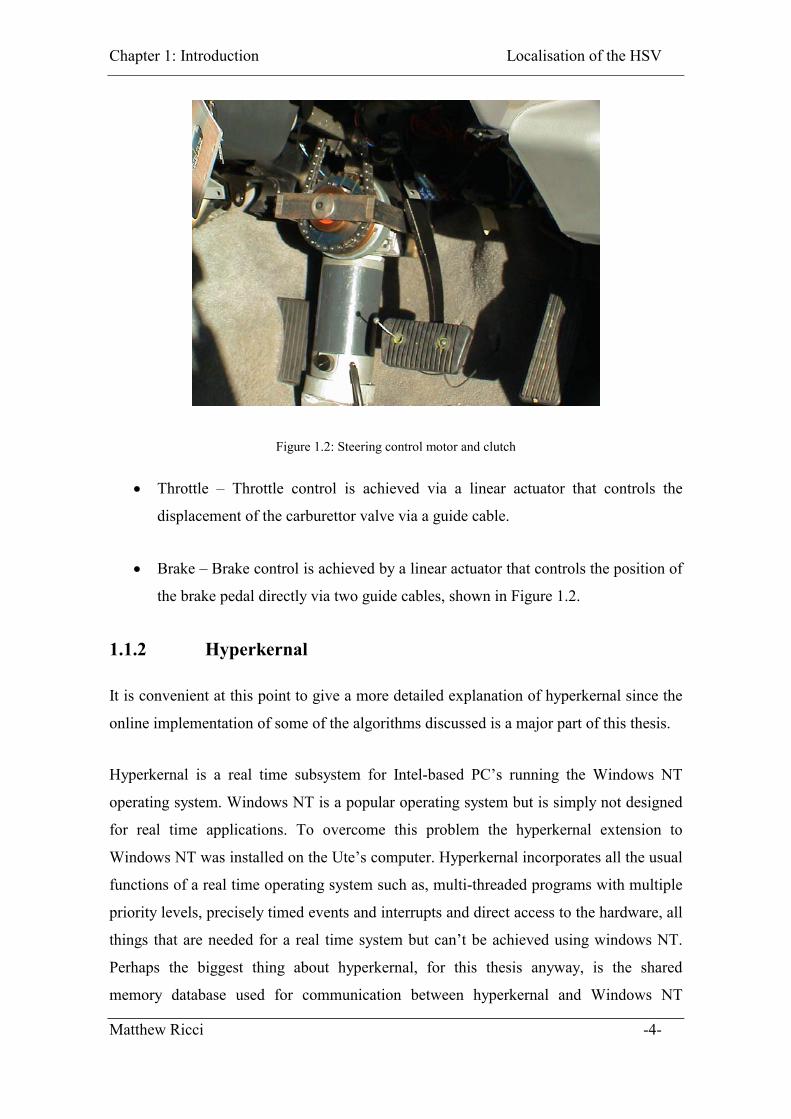
�� Steering – A 24V DC motor mounted next to the brake pedal (shown in Figure
1.2), is coupled directly onto the steering column via and electromagnetic clutch,
to directly control the position of the steering wheel.
Matthew Ricci -3-
Chapter 1: Introduction Localisation of the HSV
Figure 1.2: Steering control motor and clutch
�� Throttle – Throttle control is achieved via a linear actuator that controls the
displacement of the carburettor valve via a guide cable.
�� Brake – Brake control is achieved by a linear actuator that controls the position of
the brake pedal directly via two guide cables, shown in Figure 1.2.
1.1.2 Hyperkernal
It is convenient at this point to give a more detailed explanation of hyperkernal since the
online implementation of some of the algorithms discussed is a major part of this thesis.
Hyperkernal is a real time subsystem for Intel-based PC’s running the Windows NT
operating system. Windows NT is a popular operating system but is simply not designed
for real time applications. To overcome this problem the hyperkernal extension to
Windows NT was installed on the Ute’s computer. Hyperkernal incorporates all the usual
functions of a real time operating system such as, multi-threaded programs with multiple
priority levels, precisely timed events and interrupts and direct access to the hardware, all
things that are needed for a real time system but can’t be achieved using windows NT.
Perhaps the biggest thing about hyperkernal, for this thesis anyway, is the shared
memory database used for communication between hyperkernal and Windows NT
Matthew Ricci -4-

Chapter 1: Introduction Localisation of the HSV
applications. Hyperkernal applications running at the highest priority level of the
processor can read or write data to the shared memory database and Windows NT
applications, running whenever Hyperkernal frees the CPU, can read or write the data
to/from the shared memory. In this way hyperkernal applications and Windows NT
applications can communicate as shown in Figure 1.3. A perfect example of this is a
hyperkernal front-end program that reads the sensors, publishing the information into the
shared memory, then a C++ program reads the shared memory and graphically displays
the sensor information.
Figure 1.3: Hyperkernal shared memory architecture
The greatest attraction of the hyperkernal system as a real time platform lies in the shared
memory communication between applications since programs can be written in the more
user friendly and graphics friendly Matlab and run online on the vehicle. Also the
Windows environment makes programs easier to run and debug. However Hyperkernal
has some flaws the most obvious being that the system is very particular in that it only
runs on Windows NT platforms and cannot be ported to other Windows operating
systems such as Windows 2000 or XP. Hence any code developed on the hyperkernal
system must be changed significantly before being ported to another operating system.
Also any code that must run in the Hyperkernal part of the operating system must be
Matthew Ricci -5-
Chapter 1: Introduction Localisation of the HSV
written in C and not C++. Despite its shortcomings hyperkernal was used as the base for
the development and implementation of all the algorithms discussed in this thesis.
1.1.3 Past and Current Work
Since it’s inception in 1997 large and varied amounts of research have been carried out
on the HSV project using the Ute as a test platform. In the early stages, most of the work
was focussed upon installing hardware and writing drivers to allow for efficient operation
of the sensors and actuators. Much work has also been done on the low-level control
aspects of the vehicles actuators, ensuring that the basic framework for autonomous
navigation has been in place. More recently work has been undertaken on more high
level aspects of vehicle control such as path planning, taking into consideration vehicle
constraints, path tracking, obstacle detection using the laser and obstacle avoidance or
reactive navigation. Work has also been undertaken in the area of using vision to identify
obstacles and for vehicle localisation, as well as in the simultaneous localisation and
mapping problem (SLAM).
At present the vehicle location for the high-level control modules such as path tracking
and obstacle detection and avoidance comes solely from the GPS. Apart from GPS
estimates being quite low frequency (5Hz), the GPS also suffers from other problems
such as multipath when near trees or buildings due to reflection of the buildings and or
trees or the GPS antenna being obscured by the environment. These errors make the GPS
far from robust and as such the GPS can only be used reliably for navigation in open
environments. Naturally differential GPS (DGPS) can be used to improve these errors,
however DGPS may not always be available since it involves setting up a base station
within range of the GPS receiver. As a result to allow the vehicle to operate in an
autonomous fashion it is necessary to come up with other methods of vehicle navigation
based upon the other sensors and available in real time.
1.2 Goals of this Thesis
The primary objective of this thesis is to provide a robust and reliable algorithm capable
of providing accurate position estimates of vehicle position. The method must be
available in real time so that other software modules may perform more complex tasks,
Matthew Ricci -6-

Chapter 1: Introduction Localisation of the HSV
such as path tracking, obstacle avoidance or surveillance. A strong component of this
thesis is to make the localisation routines very modular in design so that a user need have
no knowledge of how the modules compute position; it can simply read the position
information provided, given a template of how the position information is formatted and
stored in memory. Another key component of the thesis is that the localisation modules
are available in real time and as a result of this it was decided that all modules would be
coded in C for fast operation and easy portability.
1.3 Thesis Outline
This thesis consists of two main areas, first a model based dead reckoning navigation
loop is developed using a Kalman filter to fuse together position estimates based upon a
vehicle model and also absolute position data made available by the GPS. The equations
used by this process are analysed initially followed by a detailed analysis of the
navigation loop under many different conditions. Fault detection is of prime importance
to the navigation loop to ensure that even with GPS errors the navigation loop can still
provide accurate position data.
The second part of this thesis constitutes an investigation into whether the laser can be
used to provide a path estimate of vehicle motion by matching consecutive scans and
tracking objects within these scans. Features are extracted from the raw laser data using
various line and circle detection techniques and following this, a one to one mapping of
features is found using the maximal common subgraph method.
Matthew Ricci -7-
Chapter 2:
Statistical Estimation
2.1 Introduction
In any localization or Navigation technique statistical estimation plays a crucial role
since one can never be entirely sure of the vehicle position. Hence the position must be
estimated reliably and so a robust algorithm is required to do this, so as to provide the
position estimate with the least statistical error. The method used in this thesis is the
Kalman filter.
The Kalman filter essentially consists of two stages, the prediction and the update.
During the prediction stage the next state of the system is estimated based on the current
state and some control input. This process is repeated until some absolute information
about the system state is available, upon which an update is performed. The update
simply fuses together the predicted state and the observed state to provide a least squared
estimate of the vehicle state. A prime example used in this thesis is the prediction of
vehicle position based upon velocity data taken from wheel encoders and steering data
taken from the steering LVDT. The vehicle position is continually predicted using this
data until GPS information becomes available upon which an update is performed and
the data fused to provide a new position estimate of the vehicle.
This chapter simply outlines the mathematics and general principles behind the Kalman
filter and the subsequent chapters it’s application in this thesis.
Matthew Ricci -8-

Chapter 2: Statistical Estimation Localisation of the HSV
Matthew Ricci -9-
2.2 Kalman Filter
The Kalman filter is a recursive algorithm that is used to provide statistical estimates of
the system state given all the information preceding the current state. The nature of the
Kalman filter is that it will minimize the least squared error of the system state during
each iteration. The Kalman filter consists of two main stages the prediction stage,
whereby the next state of the system is predicted based upon the current vehicle state and
a system model, and the observation stage whereby the information provided by the
prediction stage is fused with some external absolute information about the system states.
The next section of this thesis will briefly outline some of the equations used to perform
the prediction and update stages of both a linear and extended a Kalman filter. (It is noted
that the equations used in the Kalman filter are well documented and for a more detailed
description the reader is referred to [7], [21] and [24].)
The prediction part of the Kalman filter is performed using a discrete time linear model,
described by Equation 2.1.
)()()1()()( kkkkk uBxFx ���
Equation 2.1
Where:
x(k) is the predicted state of the system at time k
F(k) is the state transition matrix at time k, which relates the previous state x(k-1)
to the current state x(k).
u(k) is the input control matrix at time k
B(k) is a matrix that relates the input control signals to the system states
The uncertainty of the system states is represented by a covariance matrix (P(k|k-1)) that
contains the expected values of the variance of the error at time k given all information
up to time k-1. The covariance matrix is calculated as per Equation 2.2.
)()()1|1()()1|( kkkkkkk T QFPFP �����
Equation 2.2

Chapter 2: Statistical Estimation Localisation of the HSV
Matthew Ricci -10-
Where:
P(k|k-1) is the new covariance matrix based on the model uncertainty and the
previous covariance matrix (P(k-1|k-1)).
F(k) is the state transition matrix described in Equation 2.1
Q(k) is a system noise component related to the uncertainties in the model and the
input control vector.
For each iteration of the Kalman filter, Equation 2.1 and Equation 2.2 are computed to
provide estimates of the system state and uncertainty, until some absolute information
about the system states, known as an observation, becomes available. Upon observation
the information contained in the observation is fused with the current prediction of the
system state via Equation 2.3 to produce a new estimate of the system state.
)()()1|()|( kkkkkk vWxx ���
Equation 2.3
Where:
x(k|k) is the new state after the observation
x(k|k-1) is the predicted state at time k
W(k) is a gain matrix produced by the Kalman filter
v(k) is the innovation vector
The innovation vector (v(k)) is defined as the difference between the observation of the
states at time k and the predicted value of the states at time k (Equation 2.4).
)1|()()()( ��� kkkkk xHzv
Equation 2.4
Where:
z(k) is the observation of the states at time k
H(k) is a transformation matrix that relates the states to the observations since
generally not all states are observed.
x(k|k-1) is the predicted value of the state at time k obtained from Equation 2.1.
Chapter 2: Statistical Estimation Localisation of the HSV
Matthew Ricci -11-
From Equation 2.3 it is clear that the updated state is simply the predicted state plus some
weighting of the innovation vector. This weighting is known as the Kalman gain and is
calculated so as to minimise the least squared error of the new state estimate (Equation
2.5).
)()()1|()( 1 kkkkk T �
�� SHPW
Equation 2.5
Where:
P(k|k-1) is the current covariance matrix
H(k) is the matrix that relates he observations to the states (Equation 2.4)
S(k) is a matrix known as the innovation covariance
The innovation of the covariance is calculated by Equation 2.6.
)()()1|()()( kkkkkk T RHPHS ���
Equation 2.6
Where:
R(k) is a noise matrix associated with the observation
After the prediction information has been fused with the observation an updated
covariance or uncertainty matrix must be calculated (Equation 2.7).
)()()())()()(1|())()(()|( kkkkkkkkkkk TT WRWHWIPHWIP �����
Equation 2.7
The equations above describe the recursive Kalman filter algorithm when applied to a
linear model that can be described by Equation 2.1. However in a large number of
situations processes behave non-linearly or cannot be linearised efficiently and so the
Extended Kalman filter was developed to handle such instances.

Chapter 2: Statistical Estimation Localisation of the HSV
Matthew Ricci -12-
2.3 Extended Kalman Filter
Similar to the Kalman filter the extended Kalman filter has a prediction stage followed
by an update stage with the main difference being found in the fact that the model is now
non-linear and hence the equations describing the filter are significantly different. The
following section describes the equations behind an extended Kalman filter.
For a non-linear system the state prediction equation is shown in Equation 2.8.
))(),1|1(()1|( kkkkk uxFx ����
Equation 2.8
Where:
F(x(k-1|k-1), u(k)) is a non-linear state transition function using the current state
and a control input.
The covariance matrix after a prediction is defined in Equation 2.9.
)()()()()1|1()()1|( kkkkkkkkk TTxx BQBFPFP �������
Equation 2.9
Where:
is the Jacobian matrix of the partial derivatives of F with respect to the
state vector X.
is source error transfer matrix calculated as the Jacobian matrix of partial
derivatives of F with respect to the control input u.
Q(k) is the process noise covariance.
)(kxF�
(k)TB
Chapter 2: Statistical Estimation Localisation of the HSV
Matthew Ricci -13-
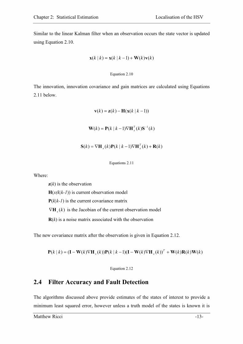
Similar to the linear Kalman filter when an observation occurs the state vector is updated
using Equation 2.10.
)()()1|()|( kkkkkk vWxx ���
Equation 2.10
The innovation, innovation covariance and gain matrices are calculated using Equations
2.11 below.
))1|(()()( ��� kkkk xHzv
)()()1|()( 1 kkkkk Tx
�
��� SHPW
)()()1|()()( kkkkkk Txx RHPHS �����
Equations 2.11
Where:
z(k) is the observation
H(x(k|k-1)) is current observation model
P(k|k-1) is the current covariance matrix
) is the Jacobian of the current observation model
R(k) is a noise matrix associated with the observation
(kxH�
The new covariance matrix after the observation is given in Equation 2.12.
)()()())()()(1|())()(()|( kkkkkkkkkkk Txx WRWHWIPHWIP �������
Equation 2.12
2.4 Filter Accuracy and Fault Detection
The algorithms discussed above provide estimates of the states of interest to provide a
minimum least squared error, however unless a truth model of the states is known it is

Chapter 2: Statistical Estimation Localisation of the HSV
Matthew Ricci -14-
unknown whether the filter is producing accurate estimates. The only information
regarding the outside world comes in the form of the observation.
For correct filter performance the innovation must have the property that it is both
unbiased and white with a covariance of S(k). To test this, the innovations are normalised
(Equation 1.13) and if the filter is operating correctly the normalised innovations are
distributed as a distribution. 2�
)()()( 1 kkkT vSv �
��
Equation 2.13
However instead of using Equation 1.13 as a check of filter performance, it could be used
as a gating function to reject wild observations. Each time the observation occurs the
value of � is checked and if it is less than some threshold the observation is accepted if
not the observation is rejected. The value of this threshold is calculated based on the
standard �2 tables based on the confidence level required. For a 95% confidence the
threshold is 12.6.

Chapter 3:
Coordinate Frames
Throughout this thesis various different coordinate frames are used to describe navigation
data. It is important to clearly define each of the frames and the transformations between
coordinate frames. A brief description of some of the coordinate systems used in this
thesis is appropriate at this point.
3.1 Earth Centred Earth Frames
Earth Centred Earth Frames or ECEF frames have their origins at the fixed to the centre
of the earth. Two major ECEF coordinate systems exist and these are rectangular ECEF
coordinates and geodetic coordinates. [7]
3.1.1 ECEF Rectangular coordinates
A standard right hand rectangular coordinate system can be defined having its origin at
the centre of the earth and is referred to as rectangular ECEF coordinates (Figure 3.1).
The x-axis extends through the intersection of the prime meridian (0� longitude) and the
equator (0� latitude). The z-axis extends through the North Pole. The y-axis completes
the set passing through the equator at 90� longitude. [7]
Matthew Ricci -15-
Chapter 3: Coordinate Frames Localisation of the HSV
Matthew Ricci -16-
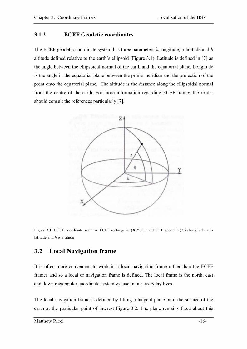
3.1.2 ECEF Geodetic coordinates
The ECEF geodetic coordinate system has three parameters � longitude, � latitude and h
altitude defined relative to the earth’s ellipsoid (Figure 3.1). Latitude is defined in [7] as
the angle between the ellipsoidal normal of the earth and the equatorial plane. Longitude
is the angle in the equatorial plane between the prime meridian and the projection of the
point onto the equatorial plane. The altitude is the distance along the ellipsoidal normal
from the centre of the earth. For more information regarding ECEF frames the reader
should consult the references particularly [7].
Figure 3.1: ECEF coordinate systems. ECEF rectangular (X,Y,Z) and ECEF geodetic (� is longitude, � is
latitude and h is altitude
3.2 Local Navigation frame
It is often more convenient to work in a local navigation frame rather than the ECEF
frames and so a local or navigation frame is defined. The local frame is the north, east
and down rectangular coordinate system we use in our everyday lives.
The local navigation frame is defined by fitting a tangent plane onto the surface of the
earth at the particular point of interest Figure 3.2. The plane remains fixed about this

Chapter 3: Coordinate Frames Localisation of the HSV
Matthew Ricci -17-
point and this point becomes the origin of the coordinate frame. The x-axis points to true
north, the y-axis points east and the z-axis points towards the centre of the earth. For this
reason the local frame is often referred to as the NED (North East Down) frame. [7]
In this thesis the NED frame is the one used to define the navigation parameters and as
such all measurements taken in the ECEF and body frames are converted to the NED
frame.
Figure 3.2: Local NED navigation frame [7]
3.3 Body Frame
Sensors reading from the vehicle are often taken with respect to the vehicle and so it is
convenient to define the body frame as a vehicle centred rectangular coordinate system or
polar coordinate system (Error! Not a valid bookmark self-reference.).
Figure 3.3: Cartesian and polar body frames

Chapter 4:
Model Based Dead Reckoning
Vehicle models can be used to make predictions about where a vehicle will be located at
a particular time given information about the vehicles current position, velocity and
steering angles. Naturally the error of such predictions will grow continually with time
due to inaccuracies in the sensors used and in the model proposed. Therefore it is
necessary not only to make predictions about vehicle states but also to have some
absolute reference about the vehicle position. In this chapter the state predictions will be
based on data from the LVDT on the steering column and the wheel encoders combined
with a vehicle model and the absolute position information will arrive via the GPS.
The data will be fused together using an extended Kalman filter to provide accurate
position estimates of the vehicle in a 2D environment.
This chapter first discusses the vehicle model used to perform the state predictions
followed by how this model is incorporated into a Kalman filter. A brief analysis of
aspects relating to filter tuning is also presented.
4.1 Vehicle Model
The vehicle model used is a simplified version of the Ackerman steering model assuming
that both wheels have the same steering angle, so in truth the model more closely
resembles a tricycle model. [9][11] Figure 4.1 shows the vehicle model used for dead
Matthew Ricci -18-
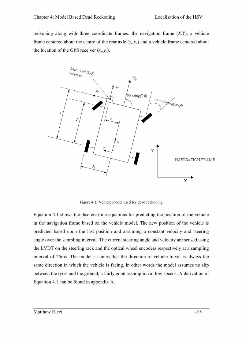
Chapter 4: Model Based Dead Reckoning Localisation of the HSV
reckoning along with three coordinate frames: the navigation frame (X,Y), a vehicle
frame centered about the centre of the rear axle (xc,yc) and a vehicle frame centered about
the location of the GPS receiver (xv,yv).
Figure 4.1: Vehicle model used for dead reckoning
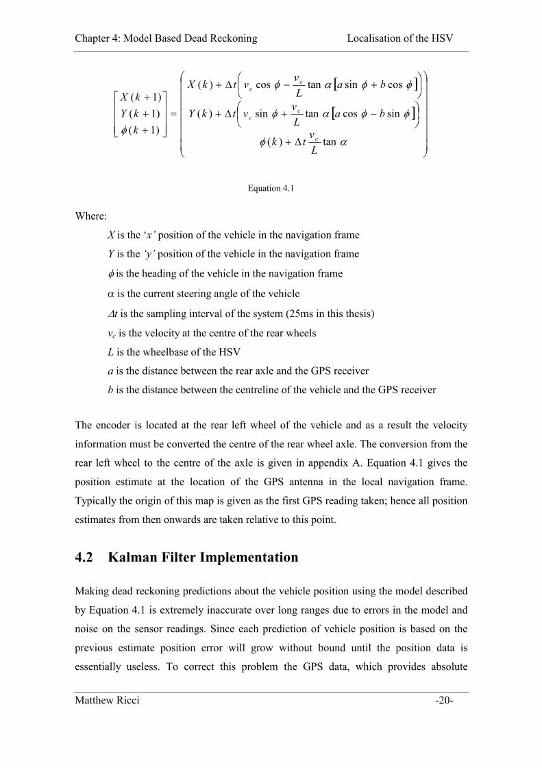
Equation 4.1 shows the discrete time equations for predicting the position of the vehicle
in the navigation frame based on the vehicle model. The new position of the vehicle is
predicted based upon the last position and assuming a constant velocity and steering
angle over the sampling interval. The current steering angle and velocity are sensed using
the LVDT on the steering rack and the optical wheel encoders respectively at a sampling
interval of 25ms. The model assumes that the direction of vehicle travel is always the
same direction in which the vehicle is facing. In other words the model assumes no slip
between the tyres and the ground, a fairly good assumption at low speeds. A derivation of
Equation 4.1 can be found in appendix A.
Matthew Ricci -19-
Chapter 4: Model Based Dead Reckoning Localisation of the HSV
� �
� �
�������
�
�
�������
�
�
��
��
���
����
��
���
����
���
�
���
�
�
�
�
�
��
����
����
�tan)(
sincostansin)(
cossintancos)(
)1()1()1(
Lvtk
baLvvtkY
baLvvtkX
kkYkX
c
cc
cc
Equation 4.1
Where:
X is the ‘x’ position of the vehicle in the navigation frame
Y is the ‘y’ position of the vehicle in the navigation frame
� is the heading of the vehicle in the navigation frame
� is the current steering angle of the vehicle
�t is the sampling interval of the system (25ms in this thesis)
vc is the velocity at the centre of the rear wheels
L is the wheelbase of the HSV
a is the distance between the rear axle and the GPS receiver
b is the distance between the centreline of the vehicle and the GPS receiver
The encoder is located at the rear left wheel of the vehicle and as a result the velocity
information must be converted the centre of the rear wheel axle. The conversion from the
rear left wheel to the centre of the axle is given in appendix A. Equation 4.1 gives the
position estimate at the location of the GPS antenna in the local navigation frame.
Typically the origin of this map is given as the first GPS reading taken; hence all position
estimates from then onwards are taken relative to this point.
4.2 Kalman Filter Implementation
Making dead reckoning predictions about the vehicle position using the model described
by Equation 4.1 is extremely inaccurate over long ranges due to errors in the model and
noise on the sensor readings. Since each prediction of vehicle position is based on the
previous estimate position error will grow without bound until the position data is
essentially useless. To correct this problem the GPS data, which provides absolute
Matthew Ricci -20-
Chapter 4: Model Based Dead Reckoning Localisation of the HSV
position information, will be fused with the model based predictions using the Kalman
filtering techniques discussed in chapter 2, Statistical Estimation.
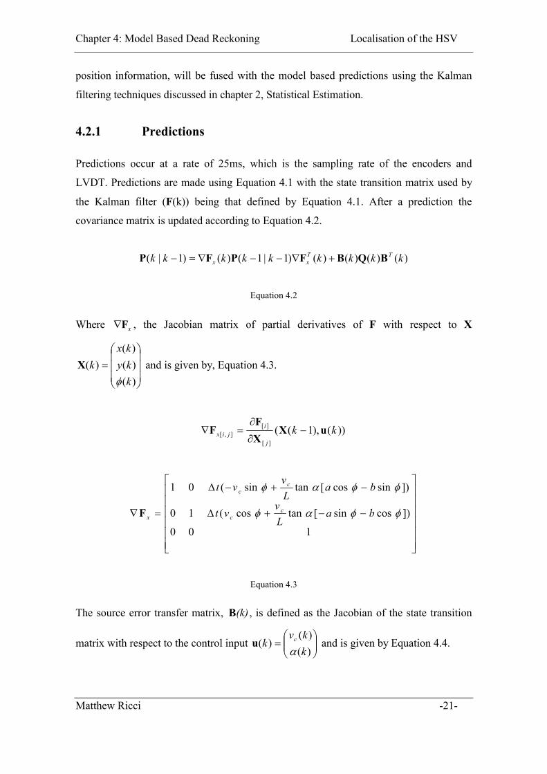
4.2.1 Predictions
Predictions occur at a rate of 25ms, which is the sampling rate of the encoders and
LVDT. Predictions are made using Equation 4.1 with the state transition matrix used by
the Kalman filter (F(k)) being that defined by Equation 4.1. After a prediction the
covariance matrix is updated according to Equation 4.2.
)()()()()1|1()()1|( kkkkkkkkk TTxx BQBFPFP �������
Equation 4.2
Where , the Jacobian matrix of partial derivatives of F with respect to X
and is given by, Equation 4.3.
xF�
���
�
�
)()()(
kkykx
� ���
�
�
�)(kX
))(),1((][
][],[ kk
j
ijix uX
XF
F ��
���
������
�
�
������
�
�
���
���
�
100
])cossin[tancos(10
])sincos[tansin(01
����
����
baLvvt
baLvvt
cc
cc
xF
Equation 4.3
The source error transfer matrix, B , is defined as the Jacobian of the state transition
matrix with respect to the control input u and is given by Equation 4.4.
(k)
���
����
��
)()(
)(kkv
k c
�
Matthew Ricci -21-
Chapter 4: Model Based Dead Reckoning Localisation of the HSV
))(),1((][
][],[ kk
j
iji uX
uF
B ��
��
������
�
�
������
�
�
���
����
�
�
���
����
���
���
�
2
2
2
costan
)sincos(cos
)sincos(tansin
)cossin(cos
)cossin(tancos
)(
Lv
L
baL
vba
baL
vba
LtkB
c
c
c
Equation 4.4
The matrix Q is a process noise covariance matrix based upon the perceived accuracy of
the encoders and the LVDT. The selection of noise values for the encoders and LVDT is
an important factor and greatly effects filter performance and is discussed in more detail
in section 4.5 Filter Tuning as well as chapter 7, Results. The process noise matrix is
given by Equation 4.5.
���
����
��
2
2
00)(steer
velk�
�Q
Equation 4.5
Where � and � represent the variance on velocity readings (m/s) taken from the
encoders and the variance on steering angle readings (rad) taken from the LVDT.
2vel
2steer
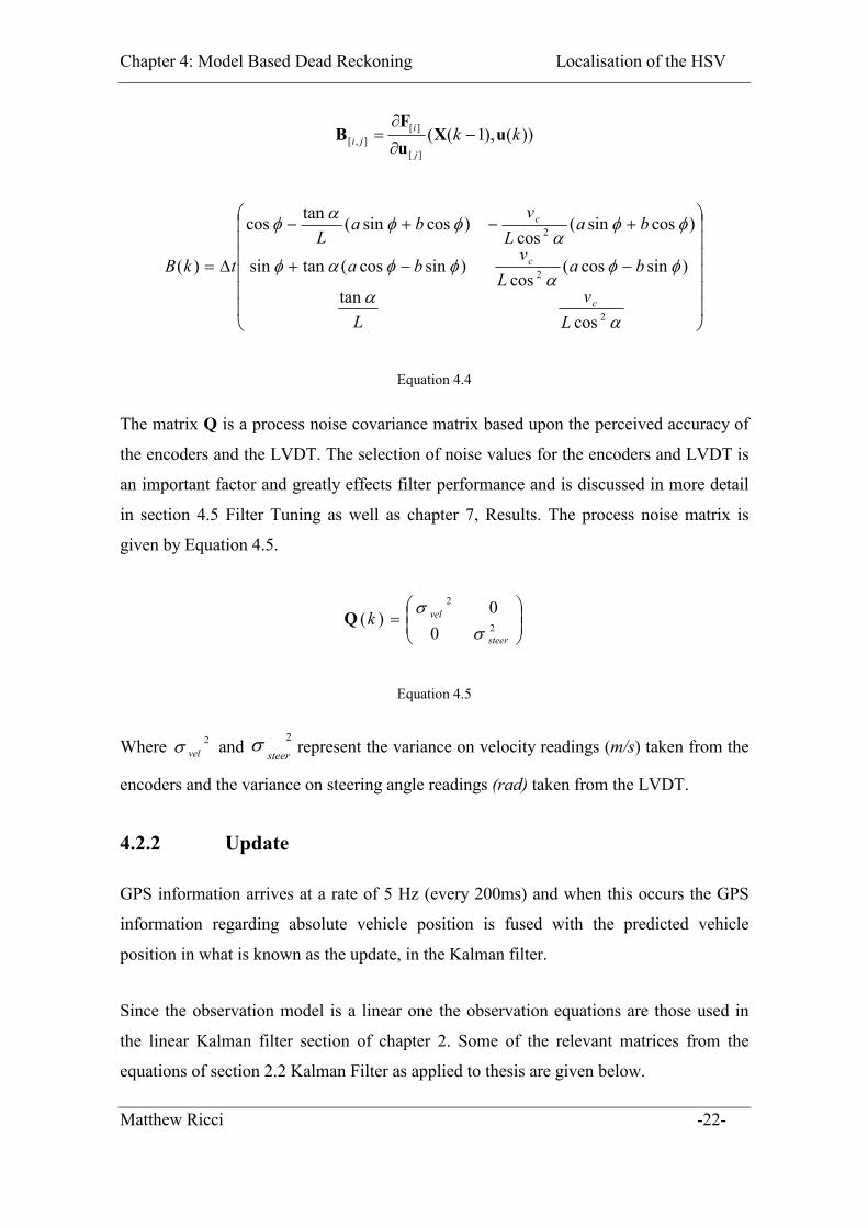
4.2.2 Update
GPS information arrives at a rate of 5 Hz (every 200ms) and when this occurs the GPS
information regarding absolute vehicle position is fused with the predicted vehicle
position in what is known as the update, in the Kalman filter.
Since the observation model is a linear one the observation equations are those used in
the linear Kalman filter section of chapter 2. Some of the relevant matrices from the
equations of section 2.2 Kalman Filter as applied to thesis are given below.
Matthew Ricci -22-
Chapter 4: Model Based Dead Reckoning Localisation of the HSV
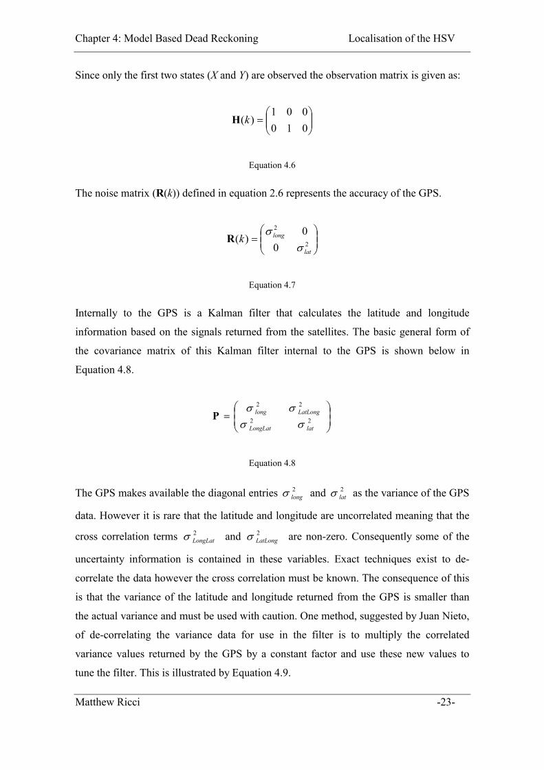
Since only the first two states (X and Y) are observed the observation matrix is given as:
���
����
��
010001
)(kH
Equation 4.6
The noise matrix (R(k)) defined in equation 2.6 represents the accuracy of the GPS.
���
����
�� 2
2
00
)(lat
longk�
�
R
Equation 4.7
Internally to the GPS is a Kalman filter that calculates the latitude and longitude
information based on the signals returned from the satellites. The basic general form of
the covariance matrix of this Kalman filter internal to the GPS is shown below in
Equation 4.8.
��
�
�
��
�
�� 22
22
latLongLat
LatLonglong
��
��
P
Equation 4.8
The GPS makes available the diagonal entries � and � as the variance of the GPS
data. However it is rare that the latitude and longitude are uncorrelated meaning that the
cross correlation terms � and � are non-zero. Consequently some of the
uncertainty information is contained in these variables. Exact techniques exist to de-
correlate the data however the cross correlation must be known. The consequence of this
is that the variance of the latitude and longitude returned from the GPS is smaller than
the actual variance and must be used with caution. One method, suggested by Juan Nieto,
of de-correlating the variance data for use in the filter is to multiply the correlated
variance values returned by the GPS by a constant factor and use these new values to
tune the filter. This is illustrated by Equation 4.9.
2long
2lat
2LongLat
2LatLong
Matthew Ricci -23-
Chapter 4: Model Based Dead Reckoning Localisation of the HSV
���
����
�� 2
2
00
*)(lat
longKk�
�
R
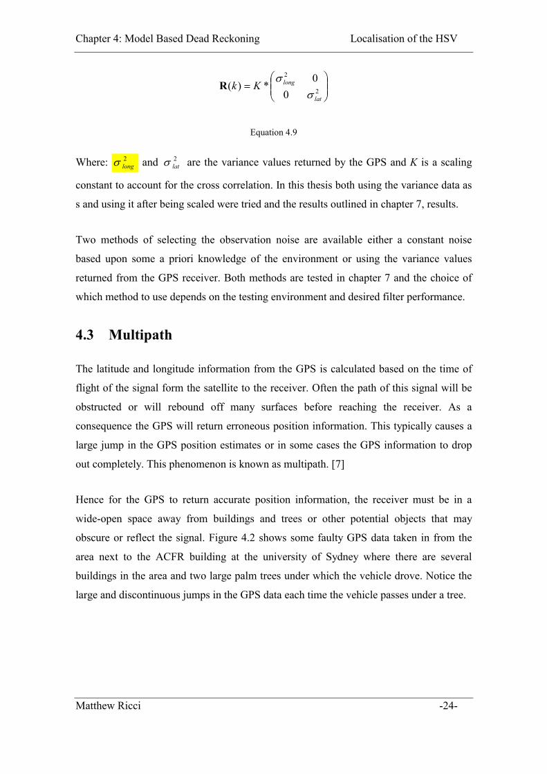
Equation 4.9
Where: and � are the variance values returned by the GPS and K is a scaling
constant to account for the cross correlation. In this thesis both using the variance data as
s and using it after being scaled were tried and the results outlined in chapter 7, results.
2long�
2lat
Two methods of selecting the observation noise are available either a constant noise
based upon some a priori knowledge of the environment or using the variance values
returned from the GPS receiver. Both methods are tested in chapter 7 and the choice of
which method to use depends on the testing environment and desired filter performance.
4.3 Multipath
The latitude and longitude information from the GPS is calculated based on the time of
flight of the signal form the satellite to the receiver. Often the path of this signal will be
obstructed or will rebound off many surfaces before reaching the receiver. As a
consequence the GPS will return erroneous position information. This typically causes a
large jump in the GPS position estimates or in some cases the GPS information to drop
out completely. This phenomenon is known as multipath. [7]
Hence for the GPS to return accurate position information, the receiver must be in a
wide-open space away from buildings and trees or other potential objects that may
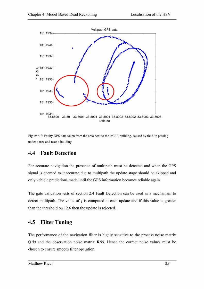
obscure or reflect the signal. Figure 4.2 shows some faulty GPS data taken in from the
area next to the ACFR building at the university of Sydney where there are several
buildings in the area and two large palm trees under which the vehicle drove. Notice the
large and discontinuous jumps in the GPS data each time the vehicle passes under a tree.
Matthew Ricci -24-
Chapter 4: Model Based Dead Reckoning Localisation of the HSV
33.8899 33.89 33.8901 33.8901 33.8901 33.8902 33.8902 33.8903 33.8903 151.1935
151.1935
151.1936
151.1936
151.1937
151.1937
151.1938
151.1939
Latitude
Longitude
Multipath GPS data
Figure 4.2: Faulty GPS data taken from the area next to the ACFR building, caused by the Ute passing
under a tree and near a building.
4.4 Fault Detection
For accurate navigation the presence of multipath must be detected and when the GPS
signal is deemed to inaccurate due to multipath the update stage should be skipped and
only vehicle predictions made until the GPS information becomes reliable again.
The gate validation tests of section 2.4 Fault Detection can be used as a mechanism to
detect multipath. The value of � is computed at each update and if this value is greater
than the threshold on 12.6 then the update is rejected.
4.5 Filter Tuning
The performance of the navigation filter is highly sensitive to the process noise matrix
Q(k) and the observation noise matrix R(k). Hence the correct noise values must be
chosen to ensure smooth filter operation.
Matthew Ricci -25-
Chapter 4: Model Based Dead Reckoning Localisation of the HSV
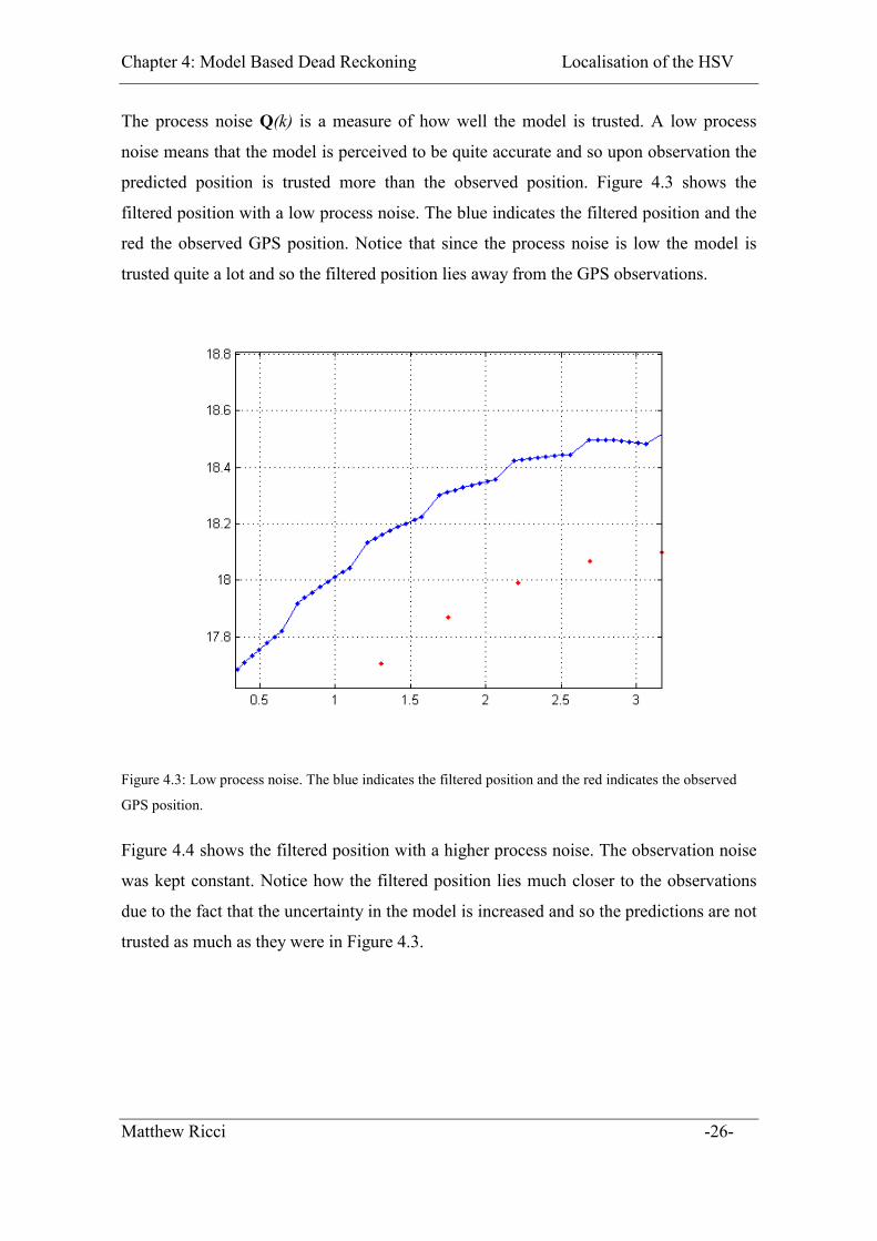
The process noise Q(k) is a measure of how well the model is trusted. A low process
noise means that the model is perceived to be quite accurate and so upon observation the
predicted position is trusted more than the observed position. Figure 4.3 shows the
filtered position with a low process noise. The blue indicates the filtered position and the
red the observed GPS position. Notice that since the process noise is low the model is
trusted quite a lot and so the filtered position lies away from the GPS observations.
Figure 4.3: Low process noise. The blue indicates the filtered position and the red indicates the observed
GPS position.
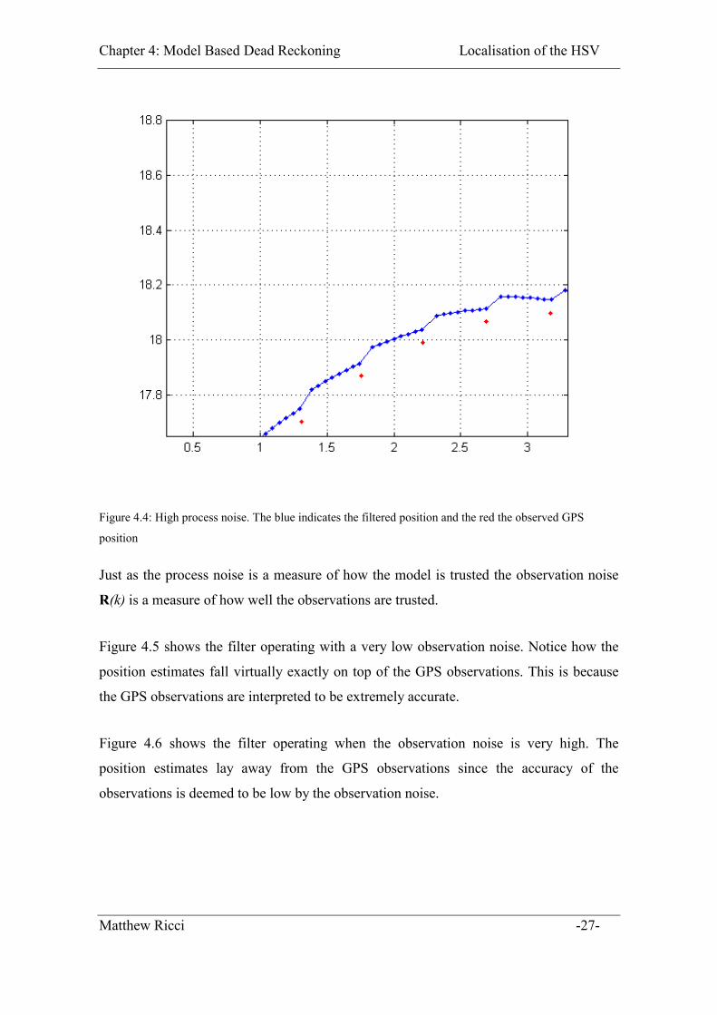
Figure 4.4 shows the filtered position with a higher process noise. The observation noise
was kept constant. Notice how the filtered position lies much closer to the observations
due to the fact that the uncertainty in the model is increased and so the predictions are not
trusted as much as they were in Figure 4.3.
Matthew Ricci -26-
Chapter 4: Model Based Dead Reckoning Localisation of the HSV
Figure 4.4: High process noise. The blue indicates the filtered position and the red the observed GPS
position
Just as the process noise is a measure of how the model is trusted the observation noise
R(k) is a measure of how well the observations are trusted.
Figure 4.5 shows the filter operating with a very low observation noise. Notice how the
position estimates fall virtually exactly on top of the GPS observations. This is because
the GPS observations are interpreted to be extremely accurate.
Figure 4.6 shows the filter operating when the observation noise is very high. The
position estimates lay away from the GPS observations since the accuracy of the
observations is deemed to be low by the observation noise.
Matthew Ricci -27-

Chapter 4: Model Based Dead Reckoning Localisation of the HSV
Figure 4.5: Low observation noise. Observed GPS data in red and filtered path estimate in blue.
Figure 4.6: Large observation noise. Estimated path in blue, observations in red.
Matthew Ricci -28-
Chapter 4: Model Based Dead Reckoning Localisation of the HSV
Clearly increasing the process noise has the same effect on filter performance as
decreasing the observation noise and similarly decreasing the process noise will have the
same effect as increasing the observation noise.
Another factor that must be considered in filter tuning is what happens to the gate
validation parameter (�) and hence the filters ability to detect and recover from the
occurrence of multipath.
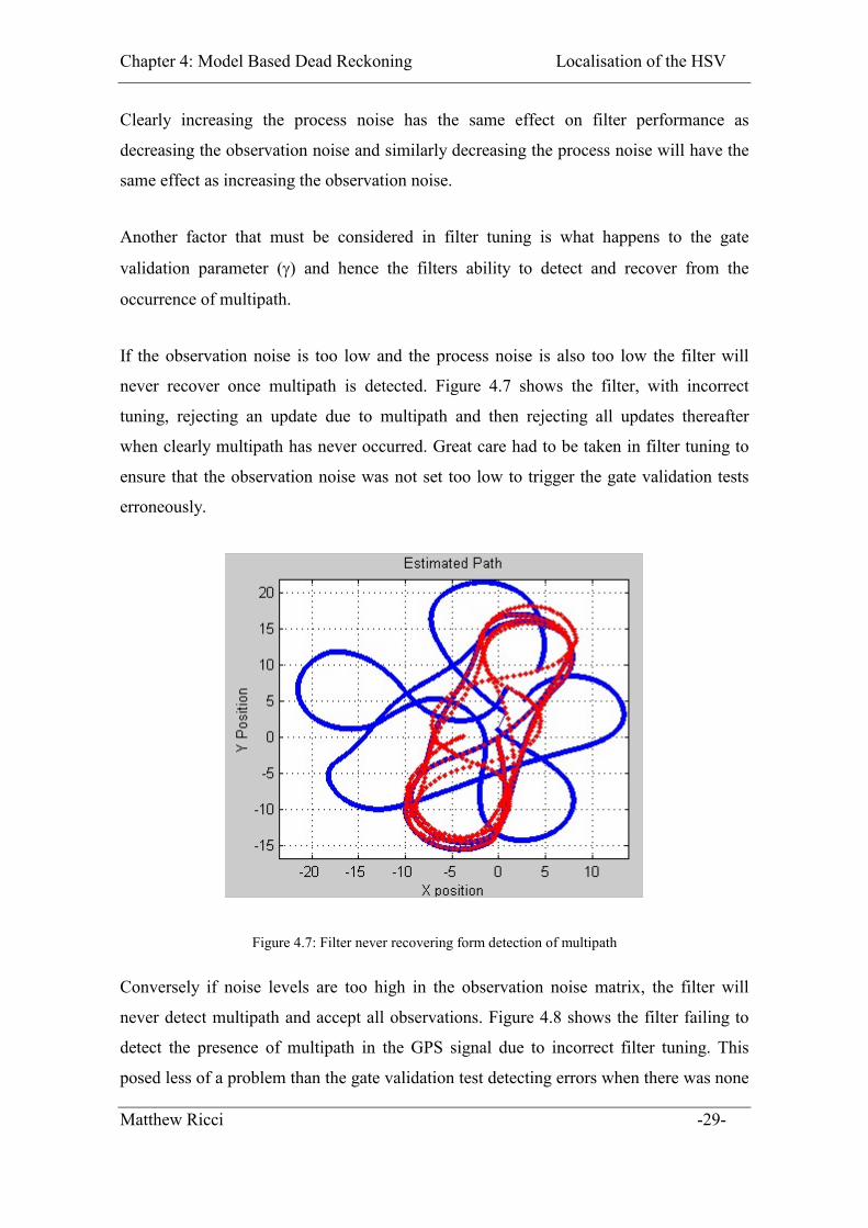
If the observation noise is too low and the process noise is also too low the filter will
never recover once multipath is detected. Figure 4.7 shows the filter, with incorrect
tuning, rejecting an update due to multipath and then rejecting all updates thereafter
when clearly multipath has never occurred. Great care had to be taken in filter tuning to
ensure that the observation noise was not set too low to trigger the gate validation tests
erroneously.
Figure 4.7: Filter never recovering form detection of multipath
Conversely if noise levels are too high in the observation noise matrix, the filter will
never detect multipath and accept all observations. Figure 4.8 shows the filter failing to
detect the presence of multipath in the GPS signal due to incorrect filter tuning. This
posed less of a problem than the gate validation test detecting errors when there was none
Matthew Ricci -29-

Chapter 4: Model Based Dead Reckoning Localisation of the HSV
since the filter generally still behaved acceptably and did not become unstable such as the
case where the filter rejects all updates (Figure 4.7).
Figure 4.8: Incorrect filter tuning failing to recognise multipath effects
4.6 Initialisation
It is very important to initialise the filter correctly. For example the initial heading may
be wrong causing the vehicle to move off in the wrong direction initially. If the filter is
tuned incorrectly it may never recover and become unstable returning essentially useless
position data. One method to correct this is to use a compass to find the initial heading
and then not accept any updates until the vehicle has started moving. A second method is
to set the initial covariance on the states (x,y,�) to be extremely large, of the order of
10km and 360� for position and heading respectively. Then once the vehicle starts
moving and a GPS update arrives the GPS information is trusted effectively 100% and
the filter will begin moving at least for a while right along the GPS path. As a
consequence it is vitally important to begin the filter in an area where the GPS data is
reliable.
Matthew Ricci -30-
Chapter 4: Model Based Dead Reckoning Localisation of the HSV
4.7 Limitations
The navigation filter presented in this chapter has several limitations associated with it.
Primarily the filter is 2-D filter and as such will not function effectively in hilly or 3-D
environments. Other methods such as inertial systems or slam must be used in 3-D
environments.
The filter is also very reliant on reliable GPS information so can only be used in
reasonably open environments. Although the filter can detect and recover from multipath
in the GPS, extended periods of GPS information being unavailable will result in the
position estimates being extremely inaccurate due to the problems in the vehicle model.
Also the module must have reliable GPS information to begin the filtering process
otherwise the origin of the map will be wrong and the navigation loop will suffer as a
result.
4.8 Conclusion
This chapter presents a 2D solution to the localisation problem utilising information
about vehicle velocity and steering angles to predict the vehicle position and then fusing
these estimates with absolute GPS position information. Reliability is guaranteed using
the gate validation to reject multipath on the GPS signals providing a more robust
navigation loop.
Matthew Ricci -31-

Chapter 5:
Laser Dead Reckoning
To date on the HSV project the 2-D range and bearing laser mounted on the Ute (see
chapter 1) has been used for a number of different applications including identification of
beacons in SLAM, 2-D and 3-D mapping of an environment and for obstacle detection in
a reactive control module. However an interesting potential application for a 2-D range
and bearing laser would be to determine vehicle pose changes from consecutive laser
scans thus providing a dead reckoning path estimate of the vehicle or an estimate of
vehicle velocity.
This chapter investigates several methods proposed for vehicle pose estimation based on
consecutive laser scans. Firstly the Iterative Closed Point method and its variants are
analysed. Following this various methods of feature extraction are discussed along with
methods of feature matching between scans. Finally once features between consecutive
scans are matched the vehicle pose change can be solved for.
5.1 Iterative Closest Point and Variations
The Iterative Closest Point (ICP) algorithm, described in greater detail in Besl & Mackay
[3] (1992) and Lu & Milios (1994) [12], is a method of comparing two consecutive laser
scans on a point-by-point basis to determine the pose transformation of the 2nd scan
relative to the first. The pose transformation of the 2nd scan relative to the 1st is equivalent
Matthew Ricci -32-
Chapter 5: Laser Dead Reckoning Localisation of the HSV
to the pose change of the vehicle. The pose change is defined as a translation in X and Y
(Tx, Ty) and a rotation (�).
For each point in the second scan the closest point in the first scan is found and these
points are matched together. Hence every point in the second scan will have a
corresponding point in the first scan. Using all these corresponding point pairs the least
squares problem is solved to produce a pose transformation of the 2nd scan relative to the
first. The data from the 2nd scan is then transposed to be relative to the first and the
process repeated until the transformation between scans converges to zero. The equations
to solve the least squares problem once points have been matched are given in Appendix
B (Equations from Lu and Milios (1994)).
Lu and Milios (1994) found that the closest point rule for matching points proved to be
very effective in detecting translational movement but not so good at detecting rotational
movement. So a second method for matching points between consecutive scans was
developed known as the Iterative Matching Range Point method (IMRP). This rule
groups points that are closest together in range. Using the iterative range point rule
proved to be effective in identifying rotational movement but not so effective in detecting
translational movement between scans.
To correct the problems of the two methods Lu and Milios (1994) developed a combined
method known as Iterative Dual Correspondence (IDC). This method took the translation
component of the ICP method and the rotational component of the IMRP method and
was found to converge much faster than both methods individually.
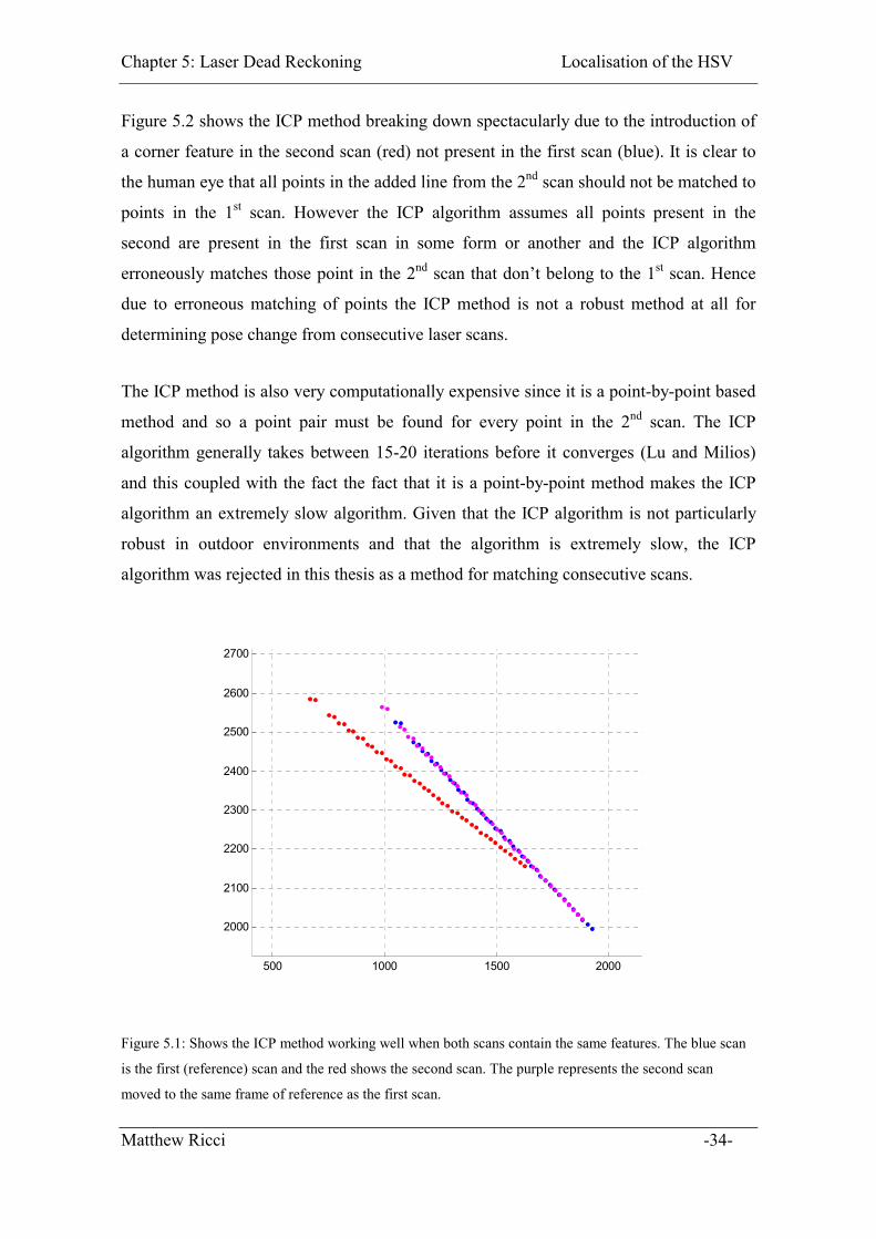
Test were conducted on the ICP methods and their variants to see if the methods could be
used to directly determine the pose change of the HSV on a point by point basis. It was
found that the ICP methods performed well if all the points present in the 2nd scan are
present in the 1st scan. Figure 5.1 shows the ICP method working well. Notice that the
amount of points and features in the first and second scans (blue and red) is practically
identical so each point in the second scan can be easily matched to the correct point in the
previous scan.
Matthew Ricci -33-
Chapter 5: Laser Dead Reckoning Localisation of the HSV
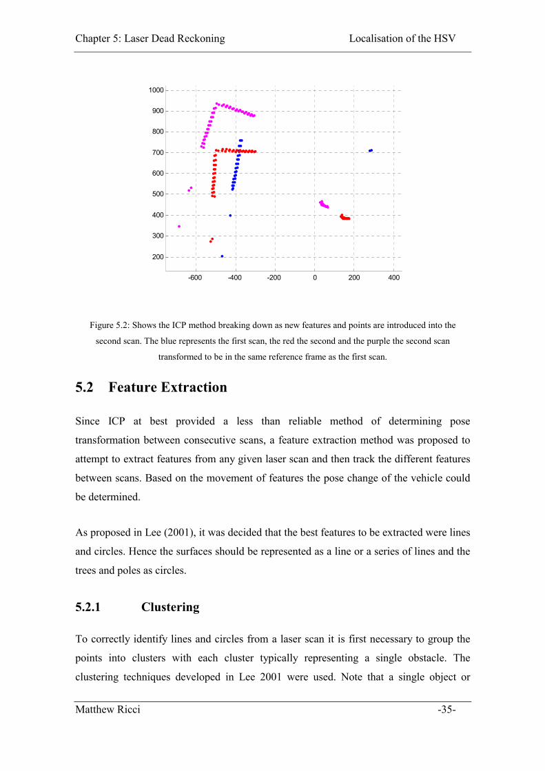
Figure 5.2 shows the ICP method breaking down spectacularly due to the introduction of
a corner feature in the second scan (red) not present in the first scan (blue). It is clear to
the human eye that all points in the added line from the 2nd scan should not be matched to
points in the 1st scan. However the ICP algorithm assumes all points present in the
second are present in the first scan in some form or another and the ICP algorithm
erroneously matches those point in the 2nd scan that don’t belong to the 1st scan. Hence
due to erroneous matching of points the ICP method is not a robust method at all for
determining pose change from consecutive laser scans.
The ICP method is also very computationally expensive since it is a point-by-point based
method and so a point pair must be found for every point in the 2nd scan. The ICP
algorithm generally takes between 15-20 iterations before it converges (Lu and Milios)
and this coupled with the fact the fact that it is a point-by-point method makes the ICP
algorithm an extremely slow algorithm. Given that the ICP algorithm is not particularly
robust in outdoor environments and that the algorithm is extremely slow, the ICP
algorithm was rejected in this thesis as a method for matching consecutive scans.
500 1000 1500 2000
2000
2100
2200
2300
2400
2500
2600
2700
Figure 5.1: Shows the ICP method working well when both scans contain the same features. The blue scan
is the first (reference) scan and the red shows the second scan. The purple represents the second scan
moved to the same frame of reference as the first scan.
Matthew Ricci -34-
Chapter 5: Laser Dead Reckoning Localisation of the HSV
-600 -400 -200 0 200 400
200
300
400
500
600
700
800
900
1000
Figure 5.2: Shows the ICP method breaking down as new features and points are introduced into the
second scan. The blue represents the first scan, the red the second and the purple the second scan
transformed to be in the same reference frame as the first scan.
5.2 Feature Extraction
Since ICP at best provided a less than reliable method of determining pose
transformation between consecutive scans, a feature extraction method was proposed to
attempt to extract features from any given laser scan and then track the different features
between scans. Based on the movement of features the pose change of the vehicle could
be determined.
As proposed in Lee (2001), it was decided that the best features to be extracted were lines
and circles. Hence the surfaces should be represented as a line or a series of lines and the
trees and poles as circles.
5.2.1 Clustering
To correctly identify lines and circles from a laser scan it is first necessary to group the
points into clusters with each cluster typically representing a single obstacle. The
clustering techniques developed in Lee 2001 were used. Note that a single object or
Matthew Ricci -35-

Chapter 5: Laser Dead Reckoning Localisation of the HSV
cluster can be represented by more than one line or circle. Recall also from chapter 1 that
the data returned from the laser is the form of an ordered array of increasing bearing
angles, with each element in the array representing the distance to the nearest object.
To form a cluster of points each point in the laser scan is compared with the previous
point in the scan and if the distance between the points is less than some threshold then
the points are assumed to part of the same object or cluster. If the point is too far away
from the previous point then a new cluster is started. Situations can arise where a point in
the laser scan fails to return a value due to a reflection of an uneven surface and when
this occurs the range reading is set to 8000, the maximum range of the laser. An example
of this is shown in Figure 5.3. If the current point is compared only to he previous points
it is clear that for the case where a pulse is lost a new cluster will be formed erroneously.
So to correct this problem the current point is compared to points that are less than three
degrees (6 bearing angles) away. Figure 5.4 shows the results of the clustering process
with each cluster shown in a different colour.
Figure 5.3: Showing the effects of how some laser pulses fail to return due to the pulse being lost
Matthew Ricci -36-
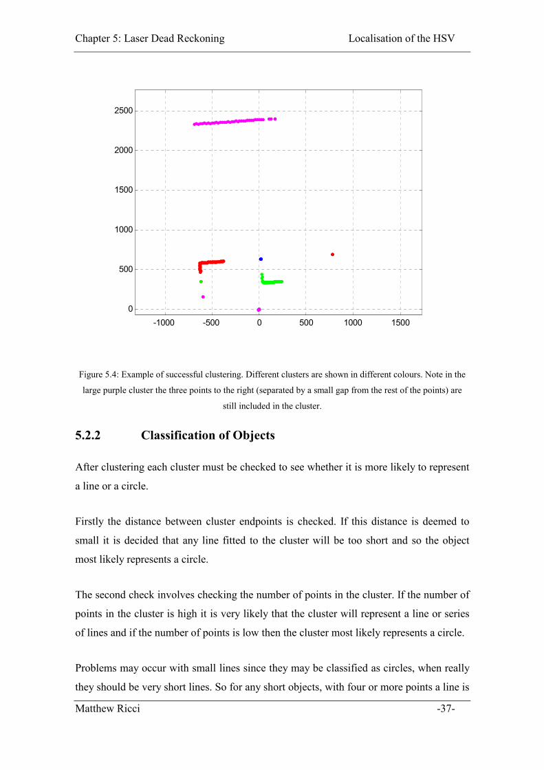
Chapter 5: Laser Dead Reckoning Localisation of the HSV
-1000 -500 0 500 1000 15000
500
1000
1500
2000
2500
Figure 5.4: Example of successful clustering. Different clusters are shown in different colours. Note in the
large purple cluster the three points to the right (separated by a small gap from the rest of the points) are
still included in the cluster.
5.2.2 Classification of Objects
After clustering each cluster must be checked to see whether it is more likely to represent
a line or a circle.
Firstly the distance between cluster endpoints is checked. If this distance is deemed to
small it is decided that any line fitted to the cluster will be too short and so the object
most likely represents a circle.
The second check involves checking the number of points in the cluster. If the number of
points in the cluster is high it is very likely that the cluster will represent a line or series
of lines and if the number of points is low then the cluster most likely represents a circle.
Problems may occur with small lines since they may be classified as circles, when really
they should be very short lines. So for any short objects, with four or more points a line is
Matthew Ricci -37-

Chapter 5: Laser Dead Reckoning Localisation of the HSV
fitted and if the quality of this line is very high (co-efficient of determination discussed in
next section was used), then a short line is fitted in place of a circle.
5.2.3 Line Detection
Fitting a line to a cluster of points provides more meaningful information about the
object and reduces the amount of data required to represent the obstacle. Lines were
decided to be a good object to fit to the raw laser data since the laser can only return the
distance to the nearest object and so, many surfaces, such as walls and cars, can easily be
represented by lines.
The method used to fit lines to a cluster of points is a statistical least squares method
aimed at reducing the square of the error of the distance of the points to the line.
Problems arise when the cluster represents more than one line as can be seen in Figure
5.4 where two of the clusters (the red and green) represent corners. Naturally when this
situation occurs multiple lines must be fitted to the cluster since one line will not
accurately describe the obstacles in the environment. This section of the report outline in
greater detail the statistical methods used for line fitting as well as the methods used to
extract multiple lines for a single cluster.
5.2.3.1 Line representation
Several methods exist for representing a line in Cartesian space. A line could be
represented using the equation of the line (y=mx+b or ax+by+c=0), the line could be
represented by its end points or the line could be represented in a polar form by a
distance to the origin r and an angle �. The polar format shown in Figure 5.5 is the one
used in this thesis since the line can be represented by two only parameters R and �. Also
the polar format is convenient when performing calculations on pose transformation at
latter stage. The start and end points of the line are also stored mainly for graphical
display purposes.
Matthew Ricci -38-
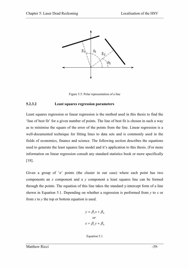
Chapter 5: Laser Dead Reckoning Localisation of the HSV
Figure 5.5: Polar representation of a line
5.2.3.2 Least squares regression parameters
Least squares regression or linear regression is the method used in this thesis to find the
‘line of best fit’ for a given number of points. The line of best fit is chosen in such a way
as to minimise the square of the error of the points from the line. Linear regression is a
well-documented technique for fitting lines to data sets and is commonly used in the
fields of economics, finance and science. The following section describes the equations
used to generate the least squares line model and it’s application to this thesis. (For more
information on linear regression consult any standard statistics book or more specifically
[18].
Given a group of ‘n’ points (the cluster in our case) where each point has two
components an x component and a y component a least squares line can be formed
through the points. The equation of this line takes the standard y-intercept form of a line
shown in Equation 5.1. Depending on whether a regression is performed from y to x or
from x to y the top or bottom equation is used.
01
01
��
��
��
��
yxor
xy
Equation 5.1
Matthew Ricci -39-

Chapter 5: Laser Dead Reckoning Localisation of the HSV
where:
�1 is the slope of the line
�0 is the intercept of the line
The slope of the line (�1) and the intercept (�0) are calculated according to the equations
below.
Regression y to x
� �01 �� �� xy
Regression x to y
� �01 �� �� yx
xy
SSSS
xx
xy
10
1
��
�
��
�
yx
SSSS
yy
xy
10
1
��
�
��
�
Where:
��
�
n
iix
nx
1
1
��
�
n
iiy
ny
1
1
nxx
xxxSS iii
n
iixx
���� ����
�
*)()( 2
1
2
nyy
yyySS iii
n
iiyy
���� ����
�
*)()( 2
1
2
nyx
yxyyxxSS iiii
n
iiixy
���� �����
�
*))((
1
The polar parameters (r,�) can be calculated from these regression parameters (�1, �2)
using simple trigonometry. For a more detailed derivation see appendix C.
Matthew Ricci -40-

Chapter 5: Laser Dead Reckoning Localisation of the HSV
)cos(),(atan2
1
0
01
21
01
��
�
��
�
��
�
�
��
�
��
rxy
xy
x
where atan2 is the 4 quadrant arctangent.
The above equation is for regression from y to x. For regression x to y simply swap
parameters x and y.
The test to determine whether to perform a regression from y to x or vice versa is based
on whether the line is more vertical or more horizontal. To determine this the values of
SSxx and SSyy are compared. If SSxx is greater than SSyy the line is more horizontal and a
regression from y to x is performed as per the equations on the left hand side above.
Otherwise a regression from x to y is performed.
The above linear regression equations provide no indication of the goodness of fit of a
line, in other words do the data points make a good line. To determine whether a line fits
the data points well we use two additional parameters about the line, the variance and the
coefficient of determination.
The coefficient of determination (R2) is a measure of how well a variation in the
independent variable can be used to predict the variation in the dependant variable. In
layman's terms the coefficient of determination is simply a measure of the linearity of the
points. The coefficient of determination always lies between 0 and 1 with 0 meaning that
there is no linear correlation in the data set and 1 being a perfect line fit. Figure 5.6
shows typical values of the coefficient of determination for three different data sets.
Matthew Ricci -41-
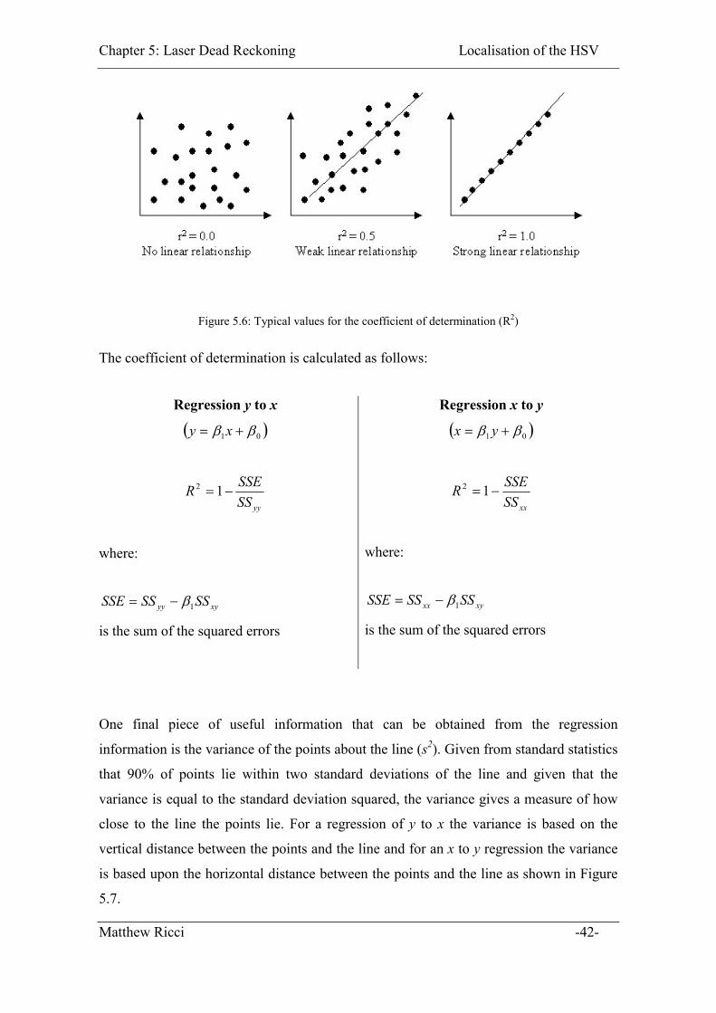
Chapter 5: Laser Dead Reckoning Localisation of the HSV
Figure 5.6: Typical values for the coefficient of determination (R2)
The coefficient of determination is calculated as follows:
Regression y to x
� �01 �� �� xy
Regression x to y
� �01 �� �� yx
yySSSSER �� 12
where:
xyyy SSSSSSE 1���
is the sum of the squared errors
xxSSSSER �� 12
where:
xyxx SSSSSSE 1���
is the sum of the squared errors
One final piece of useful information that can be obtained from the regression
information is the variance of the points about the line (s2). Given from standard statistics
that 90% of points lie within two standard deviations of the line and given that the
variance is equal to the standard deviation squared, the variance gives a measure of how
close to the line the points lie. For a regression of y to x the variance is based on the
vertical distance between the points and the line and for an x to y regression the variance
is based upon the horizontal distance between the points and the line as shown in Figure
5.7.
Matthew Ricci -42-

Chapter 5: Laser Dead Reckoning Localisation of the HSV
Figure 5.7: The variation in points from the line. On the left is the variation in y caused by a y to x
regression and on the right is the variation in x caused by an x to y regression.
The variance is calculated according to the equation below.
22
�
�
nSSEs
5.2.3.3 Coefficient of Determination Testing
Testing was done on the coefficient of determination (R2), defined in the section Least
squares regression parameters, to see if this information was useful in extracting lines
from the cluster. Given that the coefficient of determination is a measure of the linearity
of the points (Figure 5.6), it was postulated that the coefficient of determination could be
used as a basis for accepting lines or for rejecting them.
To test if the coefficient of determination was useful in extracting line information from a
cluster, a line was firstly fitted to the entire cluster and the coefficient of determination
computed for this line. If the value of R2 was less than a certain threshold, the line was
accepted and added to the list of lines for that laser scan. If the value of R2 was less than
the threshold, the cluster was bisected according to the corner method discussed in
section 5.2.3.5 Corner Method, and lines continually fitted until a suitable value of R2
was reached.
It was found that the coefficient of determination was only a useful parameter if the laser
points tested formed an almost perfect line. Figure 5.8 shows an example of a laser scan
taken from a flat surface where all the points lie nearly perfectly on the line. The
Matthew Ricci -43-
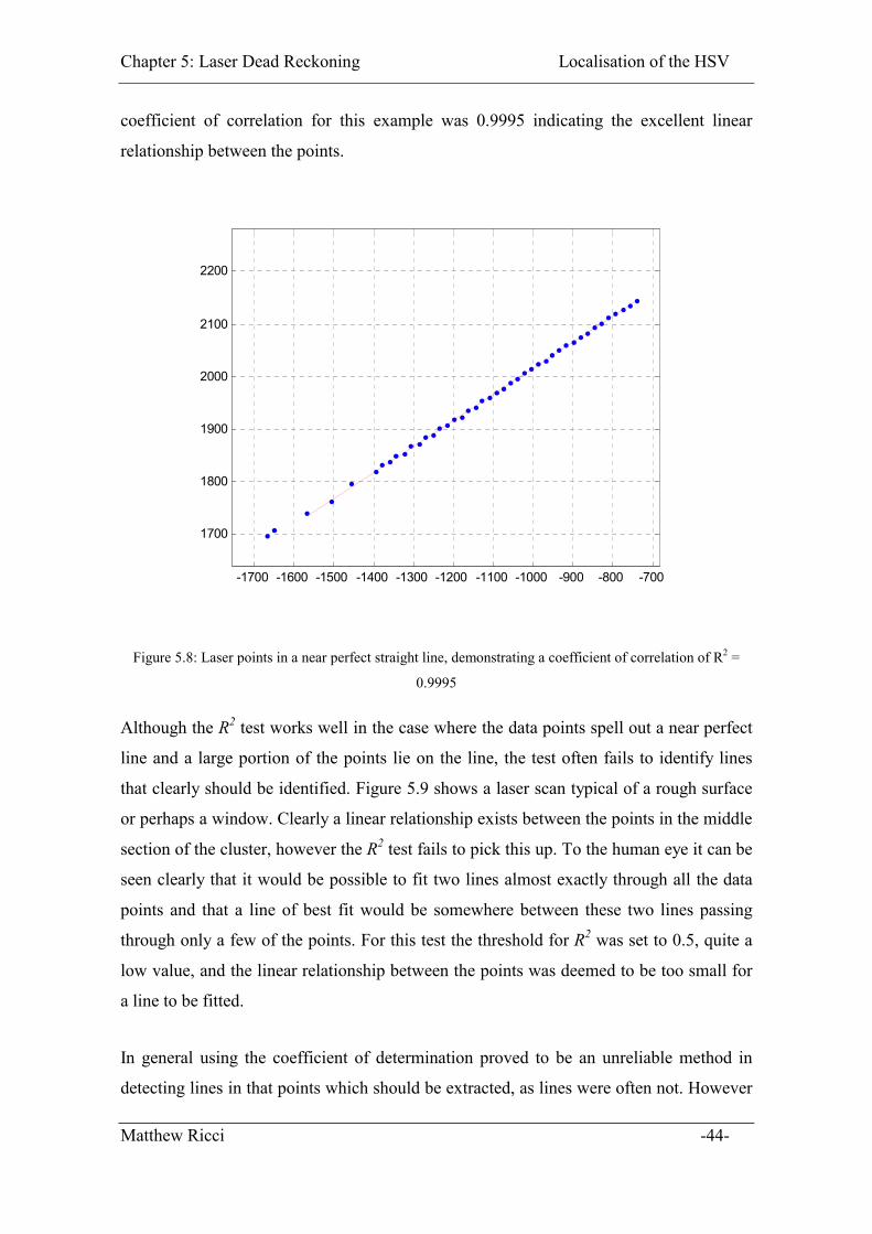
Chapter 5: Laser Dead Reckoning Localisation of the HSV
coefficient of correlation for this example was 0.9995 indicating the excellent linear
relationship between the points.
-1700 -1600 -1500 -1400 -1300 -1200 -1100 -1000 -900 -800 -700
1700
1800
1900
2000
2100
2200
Figure 5.8: Laser points in a near perfect straight line, demonstrating a coefficient of correlation of R2 =
0.9995
Although the R2 test works well in the case where the data points spell out a near perfect
line and a large portion of the points lie on the line, the test often fails to identify lines
that clearly should be identified. Figure 5.9 shows a laser scan typical of a rough surface
or perhaps a window. Clearly a linear relationship exists between the points in the middle
section of the cluster, however the R2 test fails to pick this up. To the human eye it can be
seen clearly that it would be possible to fit two lines almost exactly through all the data
points and that a line of best fit would be somewhere between these two lines passing
through only a few of the points. For this test the threshold for R2 was set to 0.5, quite a
low value, and the linear relationship between the points was deemed to be too small for
a line to be fitted.
In general using the coefficient of determination proved to be an unreliable method in
detecting lines in that points which should be extracted, as lines were often not. However
Matthew Ricci -44-
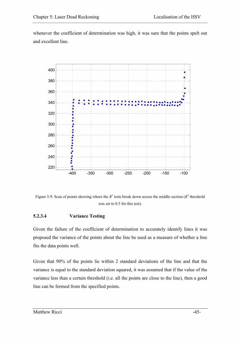
Chapter 5: Laser Dead Reckoning Localisation of the HSV
whenever the coefficient of determination was high, it was sure that the points spelt out
and excellent line.
-400 -350 -300 -250 -200 -150 -100220
240
260
280
300
320
340
360
380
400
Figure 5.9: Scan of points showing where the R2 tests break down across the middle section (R2 threshold
was set to 0.5 for this test).
5.2.3.4 Variance Testing
Given the failure of the coefficient of determination to accurately identify lines it was
proposed the variance of the points about the line be used as a measure of whether a line
fits the data points well.
Given that 90% of the points lie within 2 standard deviations of the line and that the
variance is equal to the standard deviation squared, it was assumed that if the value of the
variance less than a certain threshold (i.e. all the points are close to the line), then a good
line can be formed from the specified points.
Matthew Ricci -45-
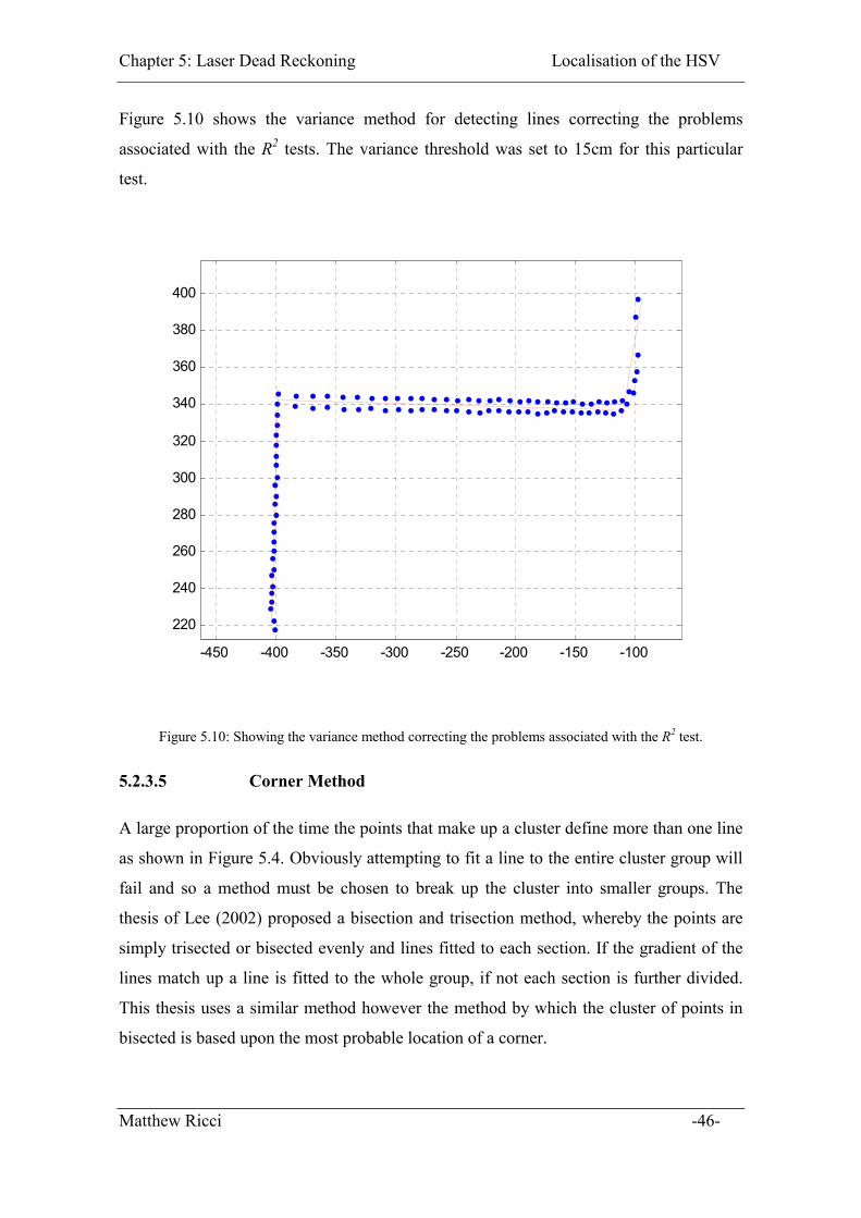
Chapter 5: Laser Dead Reckoning Localisation of the HSV
Figure 5.10 shows the variance method for detecting lines correcting the problems
associated with the R2 tests. The variance threshold was set to 15cm for this particular
test.
-450 -400 -350 -300 -250 -200 -150 -100
220
240
260
280
300
320
340
360
380
400
Figure 5.10: Showing the variance method correcting the problems associated with the R2 test.
5.2.3.5 Corner Method
A large proportion of the time the points that make up a cluster define more than one line
as shown in Figure 5.4. Obviously attempting to fit a line to the entire cluster group will
fail and so a method must be chosen to break up the cluster into smaller groups. The
thesis of Lee (2002) proposed a bisection and trisection method, whereby the points are
simply trisected or bisected evenly and lines fitted to each section. If the gradient of the
lines match up a line is fitted to the whole group, if not each section is further divided.
This thesis uses a similar method however the method by which the cluster of points in
bisected is based upon the most probable location of a corner.
Matthew Ricci -46-
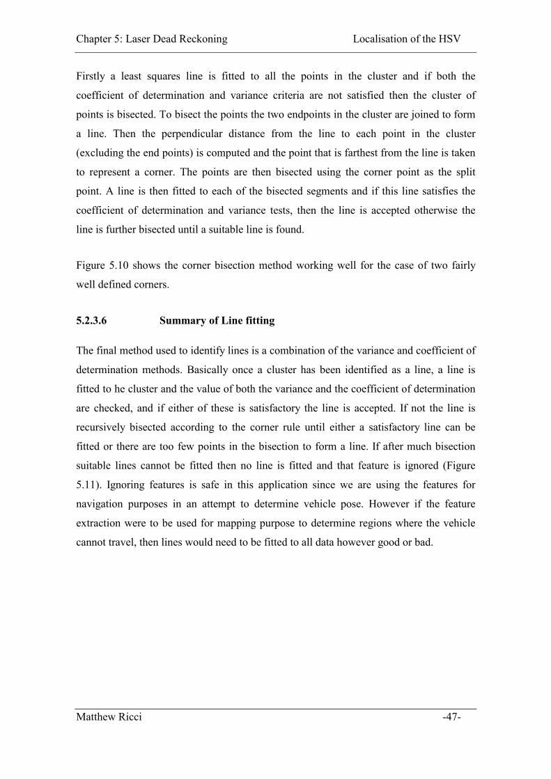
Chapter 5: Laser Dead Reckoning Localisation of the HSV
Firstly a least squares line is fitted to all the points in the cluster and if both the
coefficient of determination and variance criteria are not satisfied then the cluster of
points is bisected. To bisect the points the two endpoints in the cluster are joined to form
a line. Then the perpendicular distance from the line to each point in the cluster
(excluding the end points) is computed and the point that is farthest from the line is taken
to represent a corner. The points are then bisected using the corner point as the split
point. A line is then fitted to each of the bisected segments and if this line satisfies the
coefficient of determination and variance tests, then the line is accepted otherwise the
line is further bisected until a suitable line is found.
Figure 5.10 shows the corner bisection method working well for the case of two fairly
well defined corners.
5.2.3.6 Summary of Line fitting
The final method used to identify lines is a combination of the variance and coefficient of
determination methods. Basically once a cluster has been identified as a line, a line is
fitted to he cluster and the value of both the variance and the coefficient of determination
are checked, and if either of these is satisfactory the line is accepted. If not the line is
recursively bisected according to the corner rule until either a satisfactory line can be
fitted or there are too few points in the bisection to form a line. If after much bisection
suitable lines cannot be fitted then no line is fitted and that feature is ignored (Figure
5.11). Ignoring features is safe in this application since we are using the features for
navigation purposes in an attempt to determine vehicle pose. However if the feature
extraction were to be used for mapping purpose to determine regions where the vehicle
cannot travel, then lines would need to be fitted to all data however good or bad.
Matthew Ricci -47-
Chapter 5: Laser Dead Reckoning Localisation of the HSV
Figure 5.11: Line fitting flow chart
5.2.4 Circle Extraction
The method used to fit circles was based on the method used in the thesis of Lee 2001
developed by Jose Guivant and is detailed in the following section.
Given that the laser can only return the closest point in a surface a reflection off a circular
object such as a tree or pole will, in an ideal case, return a semi circle representing the
front half of the object (Figure 5.12). Given this information the diameter of the tree can
be estimated by simple trigonometry as shown by Figure 5.12.
RD *���
Matthew Ricci -48-
Where �� is the angle subtended by the cluster and R is the average range of the points in
the cluster.

Chapter 5: Laser Dead Reckoning Localisation of the HSV
Figure 5.12: Laser return from a typical circular object, and showing how to estimate tree diameter [7]
Guivant proposed several different methods for finding the centre of the circle. Firstly it
was assumed that the centre of the circle was collinear with the centreline of the obstacles
bearing angles, Figure 5.13. The location of the centre could then be determined in one of
two ways:
�� The distance from the point nearest the laser to the centre is equal to the radius
(Figure 5.14).
�� The distance from the average range to the centre is equal to half the radius
(Figure 5.14).
Figure 5.13: Circle Centre on centreline of bearing angles[7]
Matthew Ricci -49-
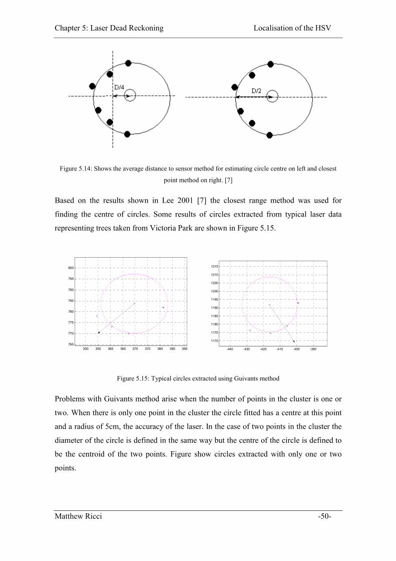
Chapter 5: Laser Dead Reckoning Localisation of the HSV
Figure 5.14: Shows the average distance to sensor method for estimating circle centre on left and closest
point method on right. [7]
Based on the results shown in Lee 2001 [7] the closest range method was used for
finding the centre of circles. Some results of circles extracted from typical laser data
representing trees taken from Victoria Park are shown in Figure 5.15.
350 355 360 365 370 375 380 385 390765
770
775
780
785
790
795
800
-440 -430 -420 -410 -400 -390
1170
1175
1180
1185
1190
1195
1200
1205
1210
1215
Figure 5.15: Typical circles extracted using Guivants method
Problems with Guivants method arise when the number of points in the cluster is one or
two. When there is only one point in the cluster the circle fitted has a centre at this point
and a radius of 5cm, the accuracy of the laser. In the case of two points in the cluster the
diameter of the circle is defined in the same way but the centre of the circle is defined to
be the centroid of the two points. Figure show circles extracted with only one or two
points.
Matthew Ricci -50-
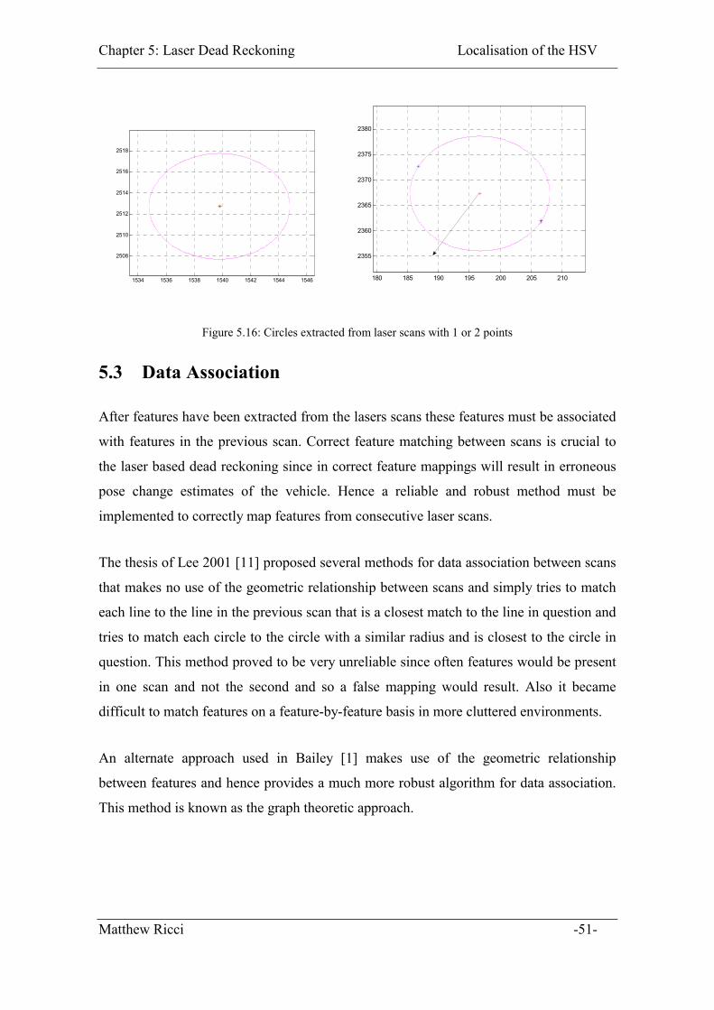
Chapter 5: Laser Dead Reckoning Localisation of the HSV
1534 1536 1538 1540 1542 1544 1546
2508
2510
2512
2514
2516
2518
180 185 190 195 200 205 210
2355
2360
2365
2370
2375
2380
Figure 5.16: Circles extracted from laser scans with 1 or 2 points
5.3 Data Association
After features have been extracted from the lasers scans these features must be associated
with features in the previous scan. Correct feature matching between scans is crucial to
the laser based dead reckoning since in correct feature mappings will result in erroneous
pose change estimates of the vehicle. Hence a reliable and robust method must be
implemented to correctly map features from consecutive laser scans.
The thesis of Lee 2001 [11] proposed several methods for data association between scans
that makes no use of the geometric relationship between scans and simply tries to match
each line to the line in the previous scan that is a closest match to the line in question and
tries to match each circle to the circle with a similar radius and is closest to the circle in
question. This method proved to be very unreliable since often features would be present
in one scan and not the second and so a false mapping would result. Also it became
difficult to match features on a feature-by-feature basis in more cluttered environments.
An alternate approach used in Bailey [1] makes use of the geometric relationship
between features and hence provides a much more robust algorithm for data association.
This method is known as the graph theoretic approach.
Matthew Ricci -51-

Chapter 5: Laser Dead Reckoning Localisation of the HSV
5.3.1 Graph Theoretic Approach
The graph theoretic approach to the data association problem essentially consists of
creating two graphs representing the features from current and previous scans and
solving the maximum common sub-graph problem for these two graphs to provide a one
to one mapping of features between consecutive scans. This section outlines the
essentials of the graph theoretic approach to the data association problem as presented in
Bailey [1].
5.3.1.1 Feature Graph Generation
The data from the feature extraction process can be represented as a graph where each
node in the graph represents a particular feature (line or circle) and each edge is the
relationship between two features. Edges must be defined for all pairs of features or
nodes and as a result the feature graph generated will have every node connected to every
other node. Logically there will be two different node types in the feature graph, lines
and circles. Therefore edges must be defined as follows: if the edge connects two lines
the edge represents the acute angle difference between the two lines, if the edge connects
a circle and a line the edge represents the perpendicular distance between the centre of
the circle and the line and for two circles the edge represents the distance between circle
centres. Figure 5.17 and Figure 5.18 show both the geometric relationship between
features and the corresponding feature graph representation for a trivial case of 2 lines
and three circles.
Matthew Ricci -52-
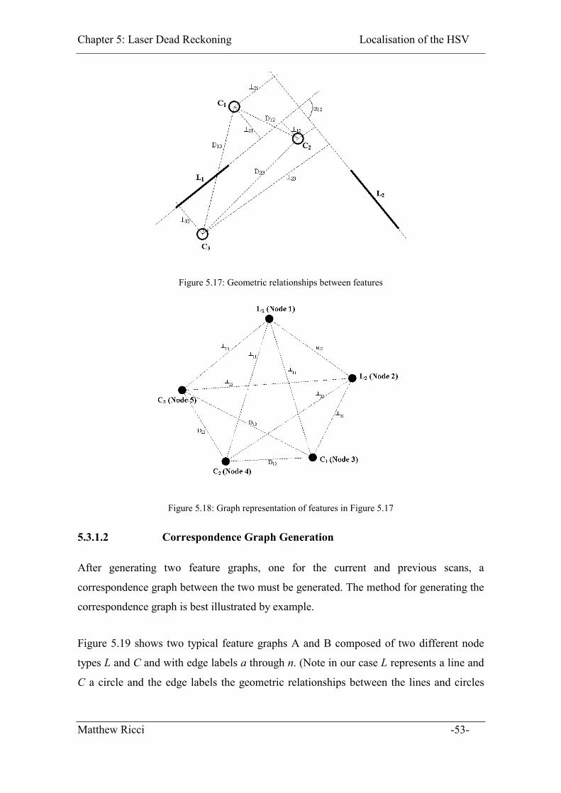
Chapter 5: Laser Dead Reckoning Localisation of the HSV
Figure 5.17: Geometric relationships between features
Figure 5.18: Graph representation of features in Figure 5.17
5.3.1.2 Correspondence Graph Generation
After generating two feature graphs, one for the current and previous scans, a
correspondence graph between the two must be generated. The method for generating the
correspondence graph is best illustrated by example.
Figure 5.19 shows two typical feature graphs A and B composed of two different node
types L and C and with edge labels a through n. (Note in our case L represents a line and
C a circle and the edge labels the geometric relationships between the lines and circles
Matthew Ricci -53-

Chapter 5: Laser Dead Reckoning Localisation of the HSV
but these node and edge labels could be generic labels for any type of graph.) Figure 5.20
shows the correspondence graph generated from graphs A and B.
To create the nodes of the correspondence graph we generate all permutations of same-
labelled nodes (nodes of the same type). For example for node type L the possible
permutations are {A1,B1}, {A1,B2}, {A2,B1}, {A2,B2}, {A3,B1} and {A3,B2}.
To generate the edges in the correspondence graph we must look for edge matches
between the two graphs. Naturally for a real system an edge value will never be exactly
the same in both scans and so edge matching will involve a certain threshold to determine
if two edges can be matched.
If an edge match is found between two similar node types (L to L or C to C), then two
edges are added to the correspondence graph. For example, in graphs A and B of Figure
5.19 the edge connecting nodes A2-A3 matches the edge connecting nodes B1-B2 and
since these pairs have the same node label (L) it is unknown whether A2 maps to B1 or to
B2. This ambiguity results in two lines being added to the correspondence graph thus
joining node 3{A2,B1} to node 6{A3,B2} and node 4{A2,B2} to node 5{A3,B1}. (Figure
5.20)
If an edge match is found between two features of different types one edge is added to
the correspondence graph. For example the edge connecting A3-A4 and the edge
connecting B2-B3 match and since A3 and B2 are both of type L and A4 and B3 are both
of type C this provides a 1 to 1 mapping of A3-B2 and A4-B3. Hence nodes 6{A3,B2} and
7{A4,B3} are joined together in the correspondence graph.
Matthew Ricci -54-
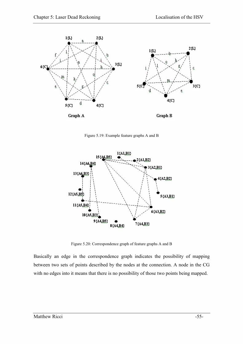
Chapter 5: Laser Dead Reckoning Localisation of the HSV
Figure 5.19: Example feature graphs A and B
Figure 5.20: Correspondence graph of feature graphs A and B
Basically an edge in the correspondence graph indicates the possibility of mapping
between two sets of points described by the nodes at the connection. A node in the CG
with no edges into it means that there is no possibility of those two points being mapped.
Matthew Ricci -55-

Chapter 5: Laser Dead Reckoning Localisation of the HSV
5.3.1.3 Maximum Clique
Bailey [1] states that finding the best mapping of features between scans is equivalent to
finding the maximal clique of the correspondence graph.
A clique is defined as a complete subgraph within a graph, in other words a subgraph in
which every node is connected to every other node. The maximum clique for the
correspondence graph is shown in Figure 5.21. The maximum clique shown indicates
that the following features were matched together {A2,B1}, {A3,B2}, {A4,B3} and
{A6,B5}.
Figure 5.21: Maximum clique of the correspondence graph
Although it easy to see the maximum clique visually it is another matter entirely to
compute the maximum clique algorithmically. The method used in this thesis was based
on a backtracking search algorithm by Bron and Kerbosch [5]. Appendix D describes this
algorithm in more detail and a code listing of the algorithm as implemented in this thesis
can be found on the CD attached to this thesis.
Matthew Ricci -56-

Chapter 5: Laser Dead Reckoning Localisation of the HSV
5.3.1.4 Effectiveness of the Graph theoretic approach
The maximal clique method for finding correspondence between features proved to be
quite effective in the majority of cases for clearly defining the best mapping between
scans. However in many cases several maximum cliques all of the same size were found
so it became difficult to determine which of these cliques contained the best mapping
solution. This was caused mainly by symmetries in the environment and occasionally by
the correspondence graph generation missing a match between graph edges. When this
occurred the maximal clique algorithm always identified the correct feature mapping
however several other false mappings were also identified with it.
Parallel lines posed quite a large problem since lines would often be paired incorrectly
due to the fact that the only matching information about lines is the angles between them.
Consider the two sets of lines in Figure 5.22, A{LA1, LA1, LA1} and B{LB1, LB1, LB1},
where scan B is imply formed by a rotation of scan A anticlockwise and a small
translation forward and to the left, giving a correct matching of {LA1,LB1}, {LA2,LB2},
{LA3,LB3}. However given that lines 1 and 2 are parallel in both scans the possibility
exists for a false mapping. During the correspondence graph generation stage the angle
between LA1 and LA2 will be correctly matched with the angle between LB1 and LB3 and
incorrectly matched to the angle between LB2 and LB3. This will causes the edges
connecting {LA1, LB2} to {LA3, LB3} and {LA1, LB3} to {LA3, LB2} to be incorrectly added to
the correspondence graph.
Whilst, for the example given in Figure 5.22, the presence of the parallel lines will not
cause an incorrect mapping, there are many cases where this will cause a problem,
especially when combined with errors relating to circle matches.
Matthew Ricci -57-
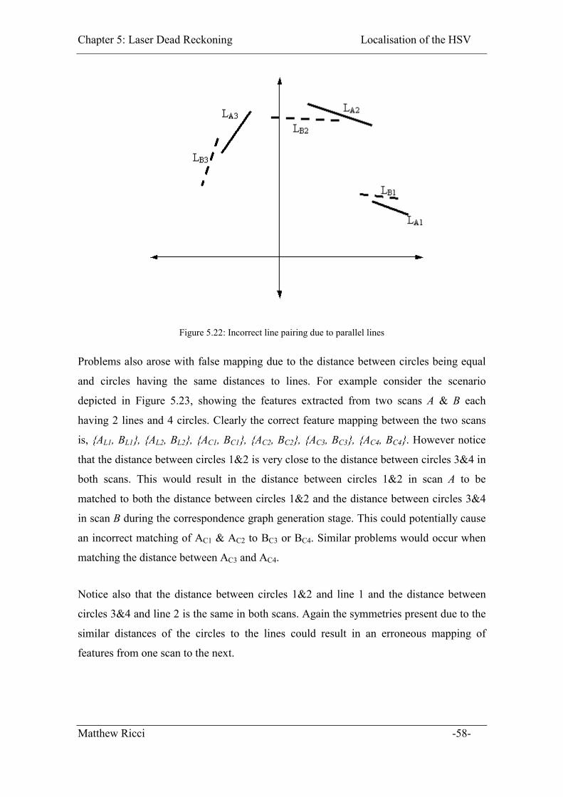
Chapter 5: Laser Dead Reckoning Localisation of the HSV
Figure 5.22: Incorrect line pairing due to parallel lines
Problems also arose with false mapping due to the distance between circles being equal
and circles having the same distances to lines. For example consider the scenario
depicted in Figure 5.23, showing the features extracted from two scans A & B each
having 2 lines and 4 circles. Clearly the correct feature mapping between the two scans
is, {AL1, BL1}, {AL2, BL2}, {AC1, BC1}, {AC2, BC2}, {AC3, BC3}, {AC4, BC4}. However notice
that the distance between circles 1&2 is very close to the distance between circles 3&4 in
both scans. This would result in the distance between circles 1&2 in scan A to be
matched to both the distance between circles 1&2 and the distance between circles 3&4
in scan B during the correspondence graph generation stage. This could potentially cause
an incorrect matching of AC1 & AC2 to BC3 or BC4. Similar problems would occur when
matching the distance between AC3 and AC4.
Notice also that the distance between circles 1&2 and line 1 and the distance between
circles 3&4 and line 2 is the same in both scans. Again the symmetries present due to the
similar distances of the circles to the lines could result in an erroneous mapping of
features from one scan to the next.
Matthew Ricci -58-
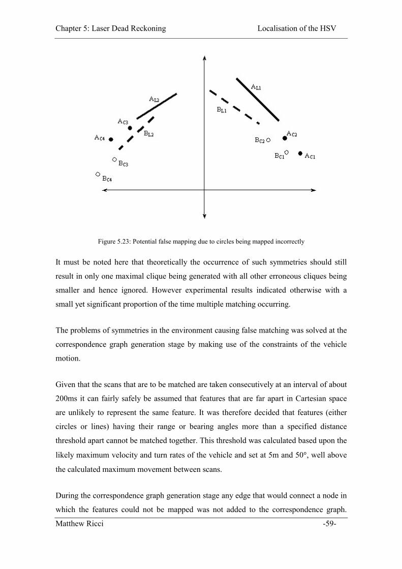
Chapter 5: Laser Dead Reckoning Localisation of the HSV
Figure 5.23: Potential false mapping due to circles being mapped incorrectly
It must be noted here that theoretically the occurrence of such symmetries should still
result in only one maximal clique being generated with all other erroneous cliques being
smaller and hence ignored. However experimental results indicated otherwise with a
small yet significant proportion of the time multiple matching occurring.
The problems of symmetries in the environment causing false matching was solved at the
correspondence graph generation stage by making use of the constraints of the vehicle
motion.
Given that the scans that are to be matched are taken consecutively at an interval of about
200ms it can fairly safely be assumed that features that are far apart in Cartesian space
are unlikely to represent the same feature. It was therefore decided that features (either
circles or lines) having their range or bearing angles more than a specified distance
threshold apart cannot be matched together. This threshold was calculated based upon the
likely maximum velocity and turn rates of the vehicle and set at 5m and 50�, well above
the calculated maximum movement between scans.
During the correspondence graph generation stage any edge that would connect a node in
which the features could not be mapped was not added to the correspondence graph.
Matthew Ricci -59-
Chapter 5: Laser Dead Reckoning Localisation of the HSV
Therefore the correspondence graph only contained edges connecting feature pairings
that were allowed by the constraints of the vehicle motion. For example consider the
scenario depicted in Figure 5.23. The distance between AC1 and AL1 would at some stage
be matched to the distance between BC3 and BL2. This would cause an edge to be added
between the nodes {AC1, BC3} and {AL1, BL2}. However since AC1 cannot be matched to
BC3 since they are too far apart and AL1 cannot be matched to BL2 then the edge is not
added to the correspondence graph. As a consequence the correspondence becomes very
sparse and a lot of memory and execution time is wasted on nodes that will never contain
an edge. Therefore an improvement on the maximal clique algorithm would be to only
generate the correspondence graph with node pairings that are allowed within the
confines of vehicle motion. Thus greatly reducing the amount of time and space required
to store and search the correspondence graph for a maximal clique.
Once the constraints of vehicle motion were taken into consideration the maximal clique
method proved to be very effective in finding the best mapping of features from
consecutive scans.
5.4 Pose Change Calculation
Once features from the current scan have been mapped to features in the previous scan it
is then necessary to compute the transformation of the current scan relative to the
previous scan. This will be equal to the change in robot pose over the interval between
scans. The transformation will be calculated based upon a rotation � and a translation Tx,
Ty. This pose transformation will be calculated in a vehicle frame and will therefore need
to be subsequently converted to the navigation frame.
A number of different methods for finding the pose transformation were used in this
thesis depending on what kinds of features were extracted from the environment. These
are outlined below.
5.4.1 Circle only Transformation
Since circles are treated as a point located at the circle centre, the only difference
between this problem and the ICP problem is that in the ICP problem the point to point
Matthew Ricci -60-
Chapter 5: Laser Dead Reckoning Localisation of the HSV
mapping of features is guessed iteratively until the best match found, whereas in this case
the point to point mapping is known via the maximal clique algorithm. Hence the pose
transformation is simply the closed form solution to the ICP problem as presented in
appendix B.
It must be noted at this point that the closed form solution for the ICP problem is only
valid if more than one pair of features is mapped between scans. Naturally the more
features that are correctly mapped the more accurate the method becomes but the method
will work for as little as two circle pairings.
5.4.2 Line only Transformation
When the only feature mapped are lines the only information that can be discerned
directly from the lines is the rotation of the vehicle since lines were modelled as infinite
segments, during the data association process. It was found that tracking line start and
endpoints was unreliable due to occlusions and other factors causing line endpoints to
move a great deal between scans.
As a result it was proposed that the intersection of lines, or corners, could also be tracked
as points features, providing the lines aren’t parallel. The point does not necessarily have
to represent an actual corner but would represent where a corner would be if the line
segments were infinite (Figure 5.24).
So for a scan in which only lines were matched, the mean rotation is calculated based
upon the change in gradient of the lines. When the average rotation is computed a simple
weighting function is used based on the variance of each line. Lines with a lower
variance are given a higher weighting and conversely lines with a higher variance are
given a lower weighting according to Equation 5.2.
���
����
���� �
��
�
n
ii
in
i i
meana
a 12
12
*1�
�
�
�
Equation 5.2
Matthew Ricci -61-
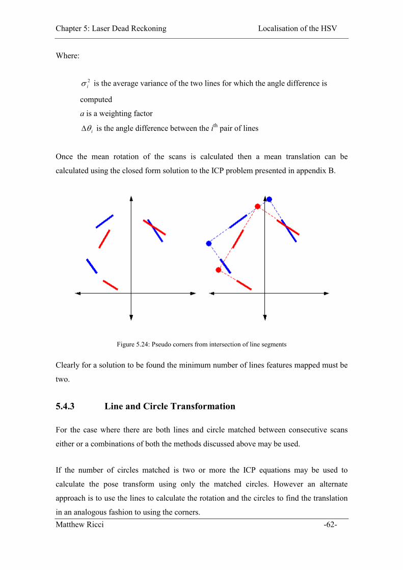
Chapter 5: Laser Dead Reckoning Localisation of the HSV
Where:
2i�
i��
is the average variance of the two lines for which the angle difference is
computed
a is a weighting factor
is the angle difference between the ith pair of lines
Once the mean rotation of the scans is calculated then a mean translation can be
calculated using the closed form solution to the ICP problem presented in appendix B.
Figure 5.24: Pseudo corners from intersection of line segments
Clearly for a solution to be found the minimum number of lines features mapped must be
two.
5.4.3 Line and Circle Transformation
For the case where there are both lines and circle matched between consecutive scans
either or a combinations of both the methods discussed above may be used.
If the number of circles matched is two or more the ICP equations may be used to
calculate the pose transform using only the matched circles. However an alternate
approach is to use the lines to calculate the rotation and the circles to find the translation
in an analogous fashion to using the corners. Matthew Ricci -62-

Chapter 5: Laser Dead Reckoning Localisation of the HSV
Based on the three method discussed above it is clear that the minimum amount of
features to get a valid solution for the pose transformation is either two circle pairings, a
pair of circles and a pair of lines or two non parallel lines. If possible the pose change is
calculated using more than one method and the average of these is taken as the pose
change of the vehicle.
5.4.4 Coordinate Transform
By summing the transformations between scans a path estimate of vehicle motion can be
built up or at the least the transformations can be combined with a timestamp to estimate
vehicle velocity. However the pose transformations are calculated in a vehicular frame
and so must be converted to the navigation frame (Figure 5.25).
Figure 5.25: Vehicle pose change in body frame
The equations to transform the translation from the body frame to the navigation frame
are given by simple trigonometry by Equation 5.3.
Matthew Ricci -63-
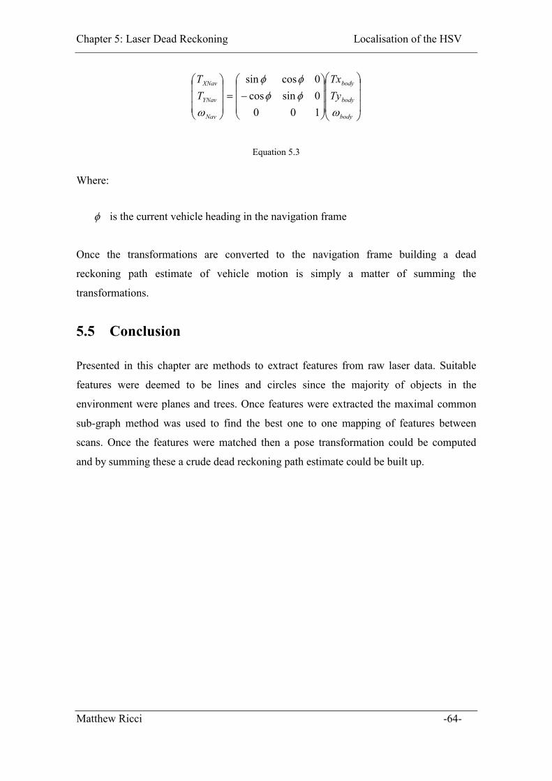
Chapter 5: Laser Dead Reckoning Localisation of the HSV
���
�
�
���
�
�
���
�
�
���
�
�
�����
�
�
���
�
�
body
body
body
Nav
YNav
XNav
TyTx
TT
�
��
��
� 1000sincos0cossin
Equation 5.3
Where:
� is the current vehicle heading in the navigation frame
Once the transformations are converted to the navigation frame building a dead
reckoning path estimate of vehicle motion is simply a matter of summing the
transformations.
5.5 Conclusion
Presented in this chapter are methods to extract features from raw laser data. Suitable
features were deemed to be lines and circles since the majority of objects in the
environment were planes and trees. Once features were extracted the maximal common
sub-graph method was used to find the best one to one mapping of features between
scans. Once the features were matched then a pose transformation could be computed
and by summing these a crude dead reckoning path estimate could be built up.
Matthew Ricci -64-
Chapter 6:
Software Implementation
This chapter outlines the different software techniques used to implement the navigation
algorithms discussed in this thesis. Firstly the kalman filter implementation for the model
based dead reckoning is discussed along with the techniques used for real time
implementation. Following this the software techniques for the laser based dead
reckoning module are discussed. Not all source code is on the data CD attached to the
rear of this thesis. Contained also on this CD is a detailed description of the code
including major functions and variable and a description of how to use the software.
6.1 Model Based Dead Reckoning
Given that the ultimate goal of this navigation loop was to implement the system in real
time, the C programming language was selected over C++ or matlab since the
hyperkernal real time operating system used on the HSV could only run C code in the
hyperkernal front end. Any C++ code had to run on the Windows NT side
communicating to the sensors via the shared memory buffer. This will be discussed in
more detail later.
The front-end program running on the HSV to read the sensors is written in C and is
implemented using several hyperkernal threads, each of which reads a particular sensor
and publishes the data into the shared memory region. [10] If written in C the code for
Matthew Ricci -65-

Chapter 6: Software Implementation Localisation of the HSV
the dead reckoning filter could easily be added to these threads to be able to run in real
time.
Given that a transition from the hyperkernal real time operating system to the QNX real
time operating system is likely to occur in 2003 a C++ offline simulation was also
developed to allow future students to easily use the filter in the future to provide position
estimates for a control module. The source code has been included on the data CD at the
back of this thesis.
6.1.1 Matrix Functions
To program a kalman filter it is necessary to have a small suite of simple matrix
functions, namely matrix multiplication, addition, subtraction, inversion and the
transpose of a matrix.
Using the algorithms in Numerical methods in C [25] a suite of basic matrix functions
was written in both C and C++. Details of the functions implemented and how to use
them can be found along with the source code on the data CD at the back of this thesis.
6.1.2 Real Time Implementation
As previously stated one of the main objectives of this thesis was to implement the
navigation filter in real time. This section discusses the communication between the
sensors and the filter in real time and the general programming concepts related to real
time programming of the filter.
The encoders, brake and throttle potentiometers and steering LVDT are all sampled at a
rate of 40 Hz or 25ms. GPS updates arrive at a rate of approximately 5Hz, 200ms. Hence
each iteration of the filter must be able to run in under 25ms in time for the next set of
prediction data to be used. Tests conducted on the Ute’s computer using an offline
simulation of the filter with sensor data arriving from a text file, indicated that the
average iteration time of the filter was under 1ms meaning that the execution time would
not pose a major problem to the running of the filter online.
Matthew Ricci -66-
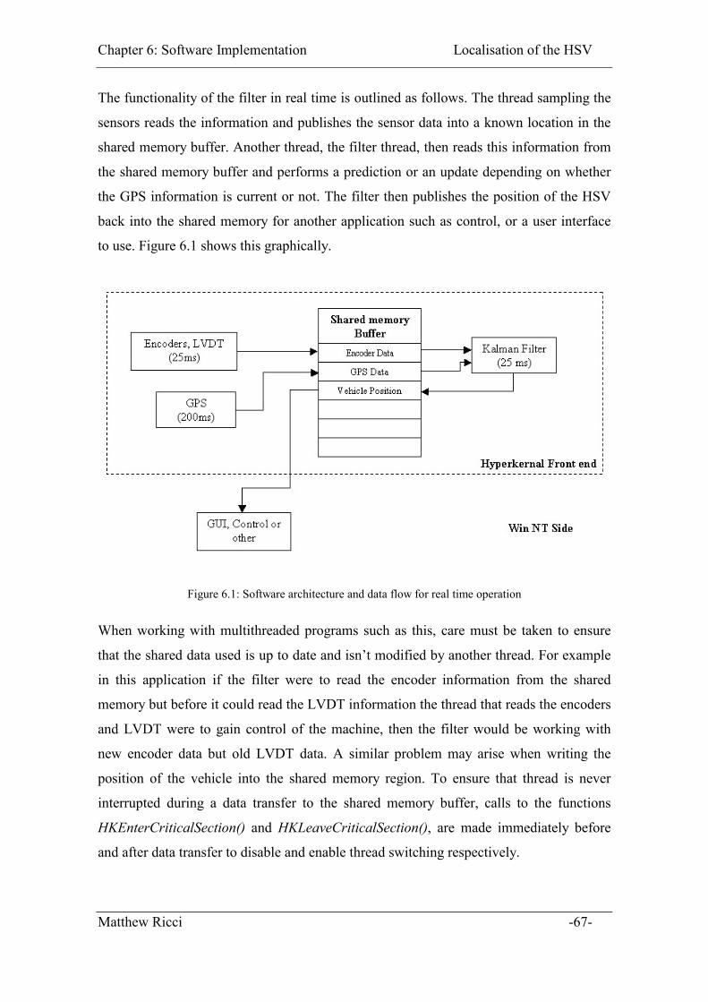
Chapter 6: Software Implementation Localisation of the HSV
The functionality of the filter in real time is outlined as follows. The thread sampling the
sensors reads the information and publishes the sensor data into a known location in the
shared memory buffer. Another thread, the filter thread, then reads this information from
the shared memory buffer and performs a prediction or an update depending on whether
the GPS information is current or not. The filter then publishes the position of the HSV
back into the shared memory for another application such as control, or a user interface
to use. Figure 6.1 shows this graphically.
Figure 6.1: Software architecture and data flow for real time operation
When working with multithreaded programs such as this, care must be taken to ensure
that the shared data used is up to date and isn’t modified by another thread. For example
in this application if the filter were to read the encoder information from the shared
memory but before it could read the LVDT information the thread that reads the encoders
and LVDT were to gain control of the machine, then the filter would be working with
new encoder data but old LVDT data. A similar problem may arise when writing the
position of the vehicle into the shared memory region. To ensure that thread is never
interrupted during a data transfer to the shared memory buffer, calls to the functions
HKEnterCriticalSection() and HKLeaveCriticalSection(), are made immediately before
and after data transfer to disable and enable thread switching respectively.
Matthew Ricci -67-
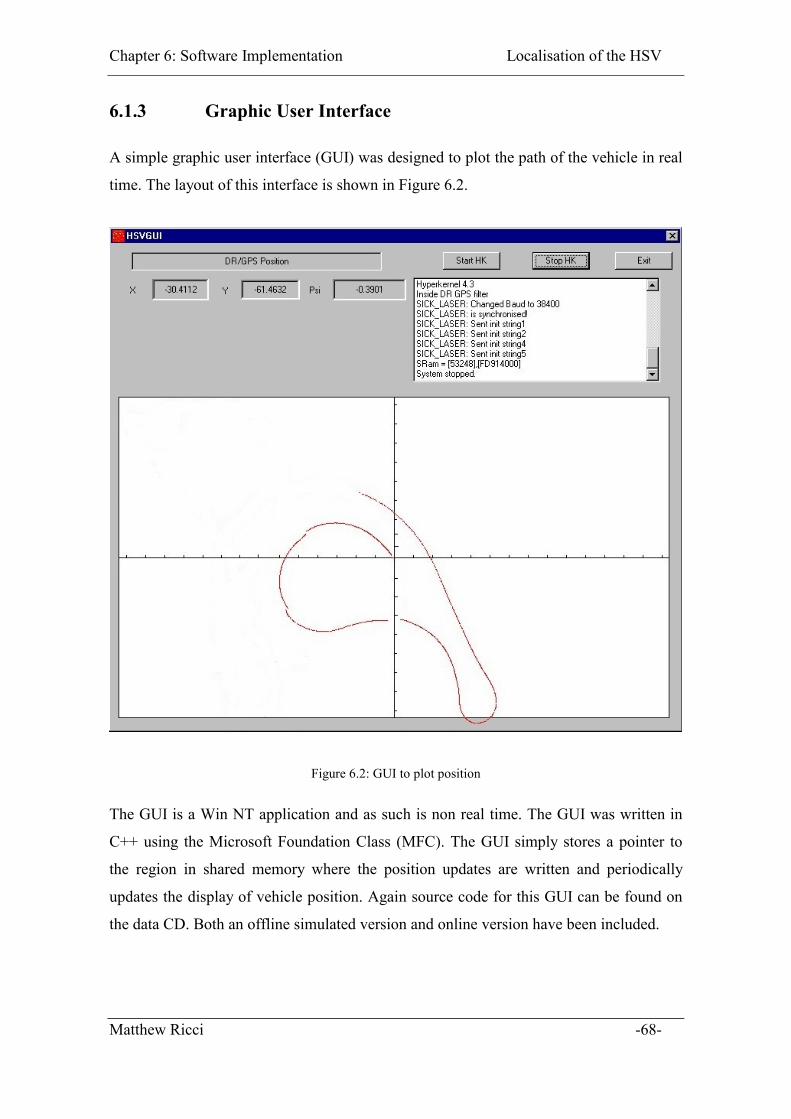
Chapter 6: Software Implementation Localisation of the HSV
6.1.3 Graphic User Interface
A simple graphic user interface (GUI) was designed to plot the path of the vehicle in real
time. The layout of this interface is shown in Figure 6.2.
Figure 6.2: GUI to plot position
The GUI is a Win NT application and as such is non real time. The GUI was written in
C++ using the Microsoft Foundation Class (MFC). The GUI simply stores a pointer to
the region in shared memory where the position updates are written and periodically
updates the display of vehicle position. Again source code for this GUI can be found on
the data CD. Both an offline simulated version and online version have been included.
Matthew Ricci -68-
Chapter 6: Software Implementation Localisation of the HSV
6.2 Laser Based dead reckoning
This next section discusses some of the software techniques used to implement the
algorithms for laser dead reckoning as presented in chapter 5.
For the same reasons as the model-based dead reckoning the laser-based dead reckoning
module was coded using the C programming language. However due to some of the
constraints of the algorithms (discussed in chapter 5&7) it was not possible to put this
module into real time operation on the Ute.
Again an outline of the functions used and major variables has been included on the data
CD for the interested reader. However a brief mention about graph representation in
software is discussed.
6.2.1 Graph Representation
[23] proposes two methods for representing a graph. The first is using a connectivity
matrix of size mxm where m is the number of nodes in the graph. If two graph nodes are
connected then a one is placed in the correct place of the connectivity matrix. For
example if node one is connected to node two then a one is placed in elements (1,2) and
(2,1) of the connectivity matrix. In general is node i is connected to node j then elements
(i,j) and (j,i) will both be true, equal to one. From this it is clear that the connectivity
matrix will be symmetric.
The second method proposed is using an array of linked lists. An array of all nodes is set-
up and each element in the array is the head of a linked list containing all nodes to which
the head node is attached. For example consider the graph shown in Figure 6.3. An array
of four elements would be created where each element represents the head of a linked list
of node structures. Element zero of the array would represent node one. This element
would head a linked list whereby the first element in the list points to node two, the
second points to node four and the third to null to indicate no more connections. Similar
lists would be set up for each of the four nodes. This is shown graphically in Figure 6.4.
Matthew Ricci -69-
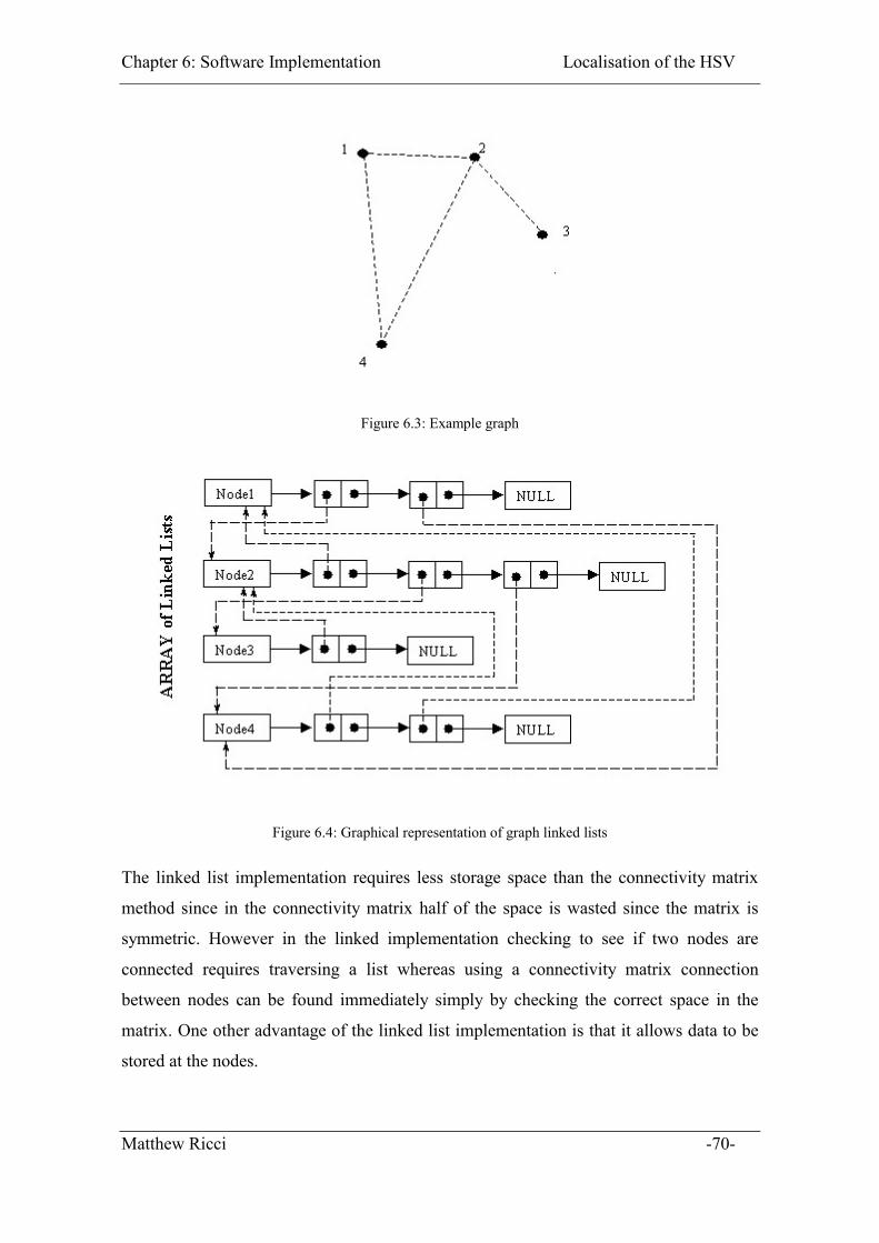
Chapter 6: Software Implementation Localisation of the HSV
Figure 6.3: Example graph
Figure 6.4: Graphical representation of graph linked lists
The linked list implementation requires less storage space than the connectivity matrix
method since in the connectivity matrix half of the space is wasted since the matrix is
symmetric. However in the linked implementation checking to see if two nodes are
connected requires traversing a list whereas using a connectivity matrix connection
between nodes can be found immediately simply by checking the correct space in the
matrix. One other advantage of the linked list implementation is that it allows data to be
stored at the nodes.
Matthew Ricci -70-

Chapter 6: Software Implementation Localisation of the HSV
Despite the advantages of the linked list implementation a connectivity matrix was used
to represent graphs in this thesis. The main reason behind this was that the maximum
clique algorithm of [5] used a connectivity matrix implementation.
Matthew Ricci -71-

Chapter 7:
Results
This chapter outlines the results of all the different algorithms discussed in this thesis.
Data from the Ute’s sensors were logged in a variety of environments around the
university. The Ute typically traveled at low speeds of less than 20km/h during testing,
mainly for safety reasons. Some of the testing locations are outlined below:
�� Seymore centre car park roof – Very open area no buildings nearby excellent GPS
reception
�� Victoria park – Many scattered trees
�� Grass area next to ACFR building – Fairly open area enclosed by buildings,
contains two large palm trees.
The a discussion of the performance of the Kalman filter discussed in chapter 4 is
presented followed by a discussion of the practicalities of using a laser based dead
reckoning procedure.
Matthew Ricci -72-
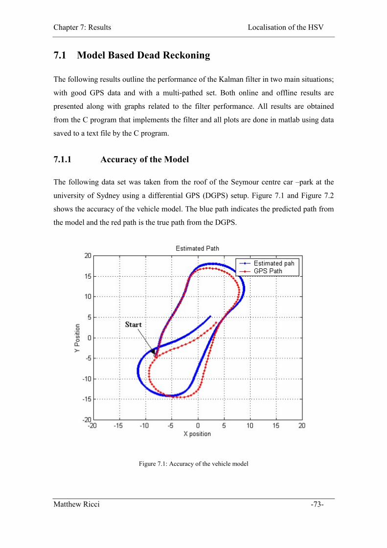
Chapter 7: Results Localisation of the HSV
7.1 Model Based Dead Reckoning
The following results outline the performance of the Kalman filter in two main situations;
with good GPS data and with a multi-pathed set. Both online and offline results are
presented along with graphs related to the filter performance. All results are obtained
from the C program that implements the filter and all plots are done in matlab using data
saved to a text file by the C program.
7.1.1 Accuracy of the Model
The following data set was taken from the roof of the Seymour centre car –park at the
university of Sydney using a differential GPS (DGPS) setup. Figure 7.1 and Figure 7.2
shows the accuracy of the vehicle model. The blue path indicates the predicted path from
the model and the red path is the true path from the DGPS.
Figure 7.1: Accuracy of the vehicle model
Matthew Ricci -73-
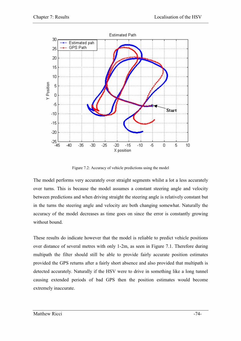
Chapter 7: Results Localisation of the HSV
Figure 7.2: Accuracy of vehicle predictions using the model
The model performs very accurately over straight segments whilst a lot a less accurately
over turns. This is because the model assumes a constant steering angle and velocity
between predictions and when driving straight the steering angle is relatively constant but
in the turns the steering angle and velocity are both changing somewhat. Naturally the
accuracy of the model decreases as time goes on since the error is constantly growing
without bound.
These results do indicate however that the model is reliable to predict vehicle positions
over distance of several metres with only 1-2m, as seen in Figure 7.1. Therefore during
multipath the filter should still be able to provide fairly accurate position estimates
provided the GPS returns after a fairly short absence and also provided that multipath is
detected accurately. Naturally if the HSV were to drive in something like a long tunnel
causing extended periods of bad GPS then the position estimates would become
extremely inaccurate.
Matthew Ricci -74-
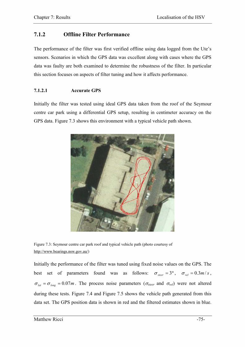
Chapter 7: Results Localisation of the HSV
7.1.2 Offline Filter Performance
The performance of the filter was first verified offline using data logged from the Ute’s
sensors. Scenarios in which the GPS data was excellent along with cases where the GPS
data was faulty are both examined to determine the robustness of the filter. In particular
this section focuses on aspects of filter tuning and how it affects performance.
7.1.2.1 Accurate GPS
Initially the filter was tested using ideal GPS data taken from the roof of the Seymour
centre car park using a differential GPS setup, resulting in centimeter accuracy on the
GPS data. Figure 7.3 shows this environment with a typical vehicle path shown.
Figure 7.3: Seymour centre car park roof and typical vehicle path (photo courtesy of
http://www.bearings.nsw.gov.au/)
Initially the performance of the filter was tuned using fixed noise values on the GPS. The
best set of parameters found was as follows: � , ,
. The process noise parameters (�
�� 3steer smvel /3.0��
mlonglat 07.0�� �� steer and �vel) were not altered
during these tests. Figure 7.4 and Figure 7.5 shows the vehicle path generated from this
data set. The GPS position data is shown in red and the filtered estimates shown in blue.
Matthew Ricci -75-

Chapter 7: Results Localisation of the HSV
The filter performed excellently providing a smooth path throughout that lay almost right
on top of the GPS information.
Notice in Figure 7.5 the saw tooth shape so typical of Kalman filters caused by the
frequent updating of the position estimates by the GPS data.
Figure 7.4: Estimated vehicle path. Data set taken from Seymore centre car park roof using DGPS. (fixed
observation noise)
Matthew Ricci -76-
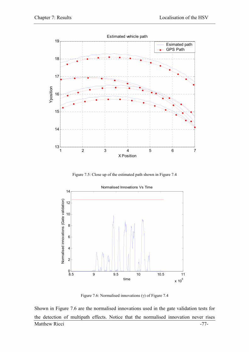
Chapter 7: Results Localisation of the HSV
1 2 3 4 5 6 713
14
15
16
17
18
19
X Position
Ypo
sitio
n
Estimated vehicle path
Esimated pathGPS Path
Figure 7.5: Close up of the estimated path shown in Figure 7.4
8.5 9 9.5 10 10.5 11
x 105
0
2
4
6
8
10
12
14
time
Nor
mal
ised
inno
vatio
ns (G
ate
valid
atio
n)
Normalised Innovations Vs Time
Figure 7.6: Normalised innovations (�) of Figure 7.4
Shown in Figure 7.6 are the normalised innovations used in the gate validation tests for
the detection of multipath effects. Notice that the normalised innovation never rises Matthew Ricci -77-
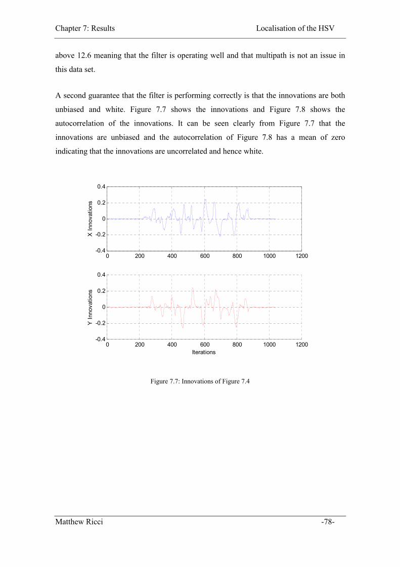
Chapter 7: Results Localisation of the HSV
above 12.6 meaning that the filter is operating well and that multipath is not an issue in
this data set.
A second guarantee that the filter is performing correctly is that the innovations are both
unbiased and white. Figure 7.7 shows the innovations and Figure 7.8 shows the
autocorrelation of the innovations. It can be seen clearly from Figure 7.7 that the
innovations are unbiased and the autocorrelation of Figure 7.8 has a mean of zero
indicating that the innovations are uncorrelated and hence white.
0 200 400 600 800 1000 1200-0.4
-0.2
0
0.2
0.4
X In
nova
tions
0 200 400 600 800 1000 1200-0.4
-0.2
0
0.2
0.4
Iterations
Y In
nova
tions
Figure 7.7: Innovations of Figure 7.4
Matthew Ricci -78-
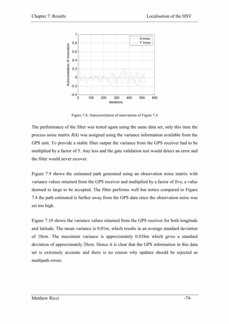
Chapter 7: Results Localisation of the HSV
0 100 200 300 400 500 600-0.4
-0.2
0
0.2
0.4
0.6
0.8
1
Iterations
Aut
ocor
rela
tion
of in
nova
tion
X innovY innov
Figure 7.8: Autocorrelation of innovations of Figure 7.4
The performance of the filter was tested again using the same data set, only this time the
process noise matrix R(k) was assigned using the variance information available from the
GPS unit. To provide a stable filter output the variance from the GPS receiver had to be
multiplied by a factor of 5. Any less and the gate validation test would detect an error and
the filter would never recover.
Figure 7.9 shows the estimated path generated using an observation noise matrix with
variance values returned from the GPS receiver and multiplied by a factor of five, a value
deemed to large to be accepted. The filter performs well but notice compared to Figure
7.4 the path estimated is further away from the GPS data since the observation noise was
set too high.
Figure 7.10 shows the variance values returned from the GPS receiver for both longitude
and latitude. The mean variance is 0.01m, which results in an average standard deviation
of 10cm. The maximum variance is approximately 0.038m which gives a standard
deviation of approximately 20cm. Hence it is clear that the GPS information in this data
set is extremely accurate and there is no reason why updates should be rejected as
multipath errors.
Matthew Ricci -79-
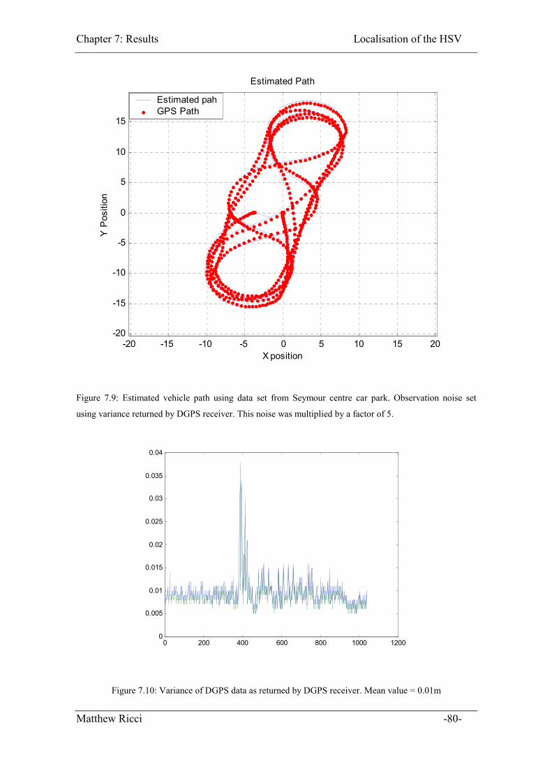
Chapter 7: Results Localisation of the HSV
-20 -15 -10 -5 0 5 10 15 20-20
-15
-10
-5
0
5
10
15
X position
Y P
ositi
on
Estimated Path
Estimated pahGPS Path
Figure 7.9: Estimated vehicle path using data set from Seymour centre car park. Observation noise set
using variance returned by DGPS receiver. This noise was multiplied by a factor of 5.
0 200 400 600 800 1000 12000
0.005
0.01
0.015
0.02
0.025
0.03
0.035
0.04
Figure 7.10: Variance of DGPS data as returned by DGPS receiver. Mean value = 0.01m
Matthew Ricci -80-
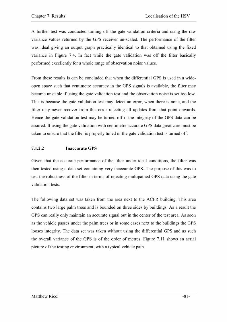
Chapter 7: Results Localisation of the HSV
A further test was conducted turning off the gate validation criteria and using the raw
variance values returned by the GPS receiver un-scaled. The performance of the filter
was ideal giving an output graph practically identical to that obtained using the fixed
variance in Figure 7.4. In fact while the gate validation was off the filter basically
performed excellently for a whole range of observation noise values.
From these results is can be concluded that when the differential GPS is used in a wide-
open space such that centimetre accuracy in the GPS signals is available, the filter may
become unstable if using the gate validation test and the observation noise is set too low.
This is because the gate validation test may detect an error, when there is none, and the
filter may never recover from this error rejecting all updates from that point onwards.
Hence the gate validation test may be turned off if the integrity of the GPS data can be
assured. If using the gate validation with centimetre accurate GPS data great care must be
taken to ensure that the filter is properly tuned or the gate validation test is turned off.
7.1.2.2 Inaccurate GPS
Given that the accurate performance of the filter under ideal conditions, the filter was
then tested using a data set containing very inaccurate GPS. The purpose of this was to
test the robustness of the filter in terms of rejecting multipathed GPS data using the gate
validation tests.
The following data set was taken from the area next to the ACFR building. This area
contains two large palm trees and is bounded on three sides by buildings. As a result the
GPS can really only maintain an accurate signal out in the center of the test area. As soon
as the vehicle passes under the palm trees or in some cases next to the buildings the GPS
looses integrity. The data set was taken without using the differential GPS and as such
the overall variance of the GPS is of the order of metres. Figure 7.11 shows an aerial
picture of the testing environment, with a typical vehicle path.
Matthew Ricci -81-
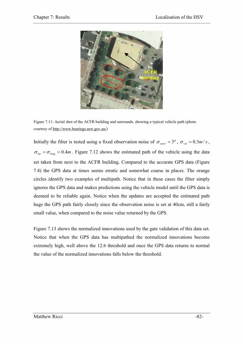
Chapter 7: Results Localisation of the HSV
ACFR building
Figure 7.11: Aerial shot of the ACFR building and surrounds, showing a typical vehicle path (photo
courtesy of http://www.bearings.nsw.gov.au/)
Initially the filter is tested using a fixed observation noise of � , � ,
. Figure 7.12 shows the estimated path of the vehicle using the data
set taken from next to the ACFR building. Compared to the accurate GPS data (Figure
7.4) the GPS data at times seems erratic and somewhat coarse in places. The orange
circles identify two examples of multipath. Notice that in these cases the filter simply
ignores the GPS data and makes predictions using the vehicle model until the GPS data is
deemed to be reliable again. Notice when the updates are accepted the estimated path
hugs the GPS path fairly closely since the observation noise is set at 40cm, still a fairly
small value, when compared to the noise value returned by the GPS.
�� 3steer smvel /3.0�
mlonglat 4.0�� ��
Figure 7.13 shows the normalized innovations used by the gate validation of this data set.
Notice that when the GPS data has multipathed the normalized innovations become
extremely high, well above the 12.6 threshold and once the GPS data returns to normal
the value of the normalized innovations falls below the threshold.
Matthew Ricci -82-
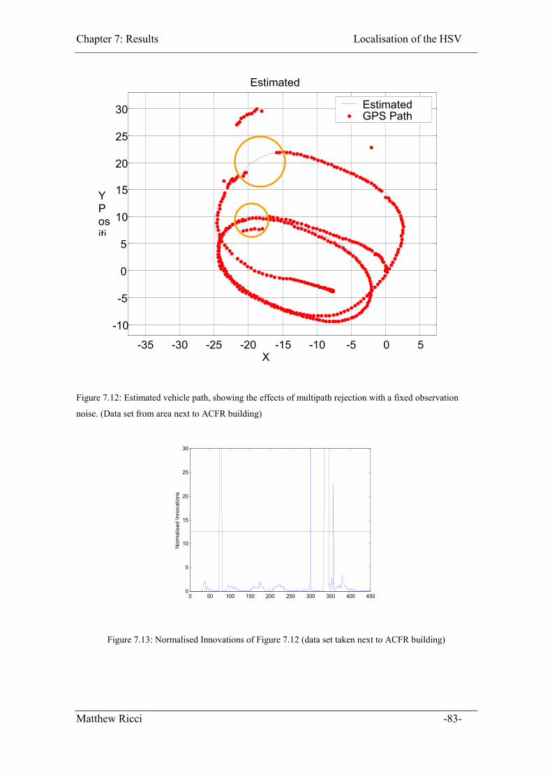
Chapter 7: Results Localisation of the HSV
-35 -30 -25 -20 -15 -10 -5 0 5
-10
-5
0
5
10
15
20
25
30
X
Y Positi
Estimated
Estimated GPS Path
Figure 7.12: Estimated vehicle path, showing the effects of multipath rejection with a fixed observation
noise. (Data set from area next to ACFR building)
0 50 100 150 200 250 300 350 400 4500
5
10
15
20
25
30
Nor
mal
ised
Inno
vatio
ns
Figure 7.13: Normalised Innovations of Figure 7.12 (data set taken next to ACFR building)
Matthew Ricci -83-
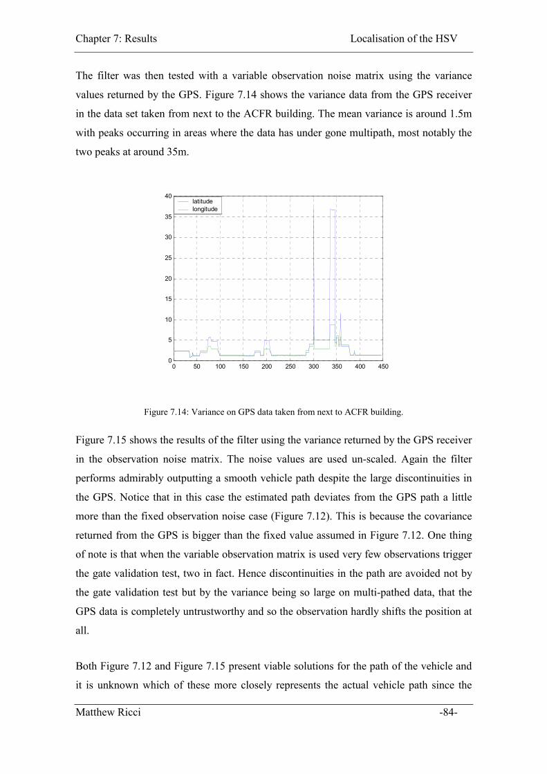
Chapter 7: Results Localisation of the HSV
The filter was then tested with a variable observation noise matrix using the variance
values returned by the GPS. Figure 7.14 shows the variance data from the GPS receiver
in the data set taken from next to the ACFR building. The mean variance is around 1.5m
with peaks occurring in areas where the data has under gone multipath, most notably the
two peaks at around 35m.
0 50 100 150 200 250 300 350 400 4500
5
10
15
20
25
30
35
40latitude longitude
Figure 7.14: Variance on GPS data taken from next to ACFR building.
Figure 7.15 shows the results of the filter using the variance returned by the GPS receiver
in the observation noise matrix. The noise values are used un-scaled. Again the filter
performs admirably outputting a smooth vehicle path despite the large discontinuities in
the GPS. Notice that in this case the estimated path deviates from the GPS path a little
more than the fixed observation noise case (Figure 7.12). This is because the covariance
returned from the GPS is bigger than the fixed value assumed in Figure 7.12. One thing
of note is that when the variable observation matrix is used very few observations trigger
the gate validation test, two in fact. Hence discontinuities in the path are avoided not by
the gate validation test but by the variance being so large on multi-pathed data, that the
GPS data is completely untrustworthy and so the observation hardly shifts the position at
all.
Both Figure 7.12 and Figure 7.15 present viable solutions for the path of the vehicle and
it is unknown which of these more closely represents the actual vehicle path since the
Matthew Ricci -84-
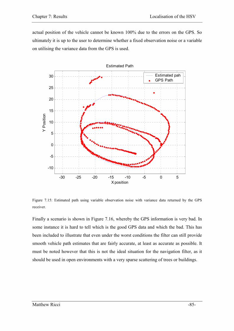
Chapter 7: Results Localisation of the HSV
actual position of the vehicle cannot be known 100% due to the errors on the GPS. So
ultimately it is up to the user to determine whether a fixed observation noise or a variable
on utilising the variance data from the GPS is used.
-30 -25 -20 -15 -10 -5 0 5
-10
-5
0
5
10
15
20
25
30
X position
Y P
ositi
on
Estimated Path
Estimated pahGPS Path
Figure 7.15: Estimated path using variable observation noise with variance data returned by the GPS
receiver.
Finally a scenario is shown in Figure 7.16, whereby the GPS information is very bad. In
some instance it is hard to tell which is the good GPS data and which the bad. This has
been included to illustrate that even under the worst conditions the filter can still provide
smooth vehicle path estimates that are fairly accurate, at least as accurate as possible. It
must be noted however that this is not the ideal situation for the navigation filter, as it
should be used in open environments with a very sparse scattering of trees or buildings.
Matthew Ricci -85-
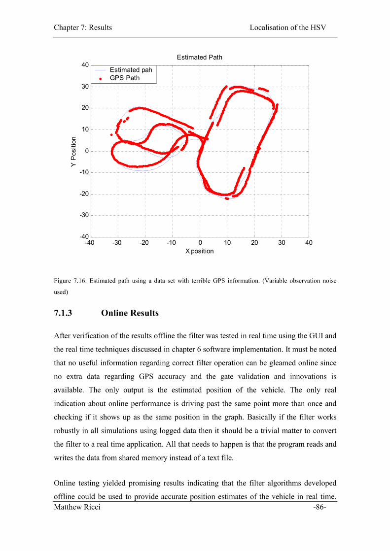
Chapter 7: Results Localisation of the HSV
-40 -30 -20 -10 0 10 20 30 40-40
-30
-20
-10
0
10
20
30
40
X position
Y P
ositi
on
Estimated Path
Estimated pahGPS Path
Figure 7.16: Estimated path using a data set with terrible GPS information. (Variable observation noise
used)
7.1.3 Online Results
After verification of the results offline the filter was tested in real time using the GUI and
the real time techniques discussed in chapter 6 software implementation. It must be noted
that no useful information regarding correct filter operation can be gleamed online since
no extra data regarding GPS accuracy and the gate validation and innovations is
available. The only output is the estimated position of the vehicle. The only real
indication about online performance is driving past the same point more than once and
checking if it shows up as the same position in the graph. Basically if the filter works
robustly in all simulations using logged data then it should be a trivial matter to convert
the filter to a real time application. All that needs to happen is that the program reads and
writes the data from shared memory instead of a text file.
Matthew Ricci -86-
Online testing yielded promising results indicating that the filter algorithms developed
offline could be used to provide accurate position estimates of the vehicle in real time.

Chapter 7: Results Localisation of the HSV
Figure 7.17 shows one such example of the filter working well in real time in the area
next to the ACFR building.
Figure 7.17: Simple vehicle path plotted online in the area next to the ACFR building
7.1.4 Summary
Given the results just discussed it is clear that the performance of this navigation loop is
highly dependant on the tuning of the Kalman filter thus it is important to tune the filter
for the specific application and environment.
The ideal value for the process noise was found to be � , , and
was based on the theoretical error of the LVDT and wheel encoders. This value was
unchanged during the tuning processes of the filter.
�� 3steer smvel /3.0��
Matthew Ricci -87-
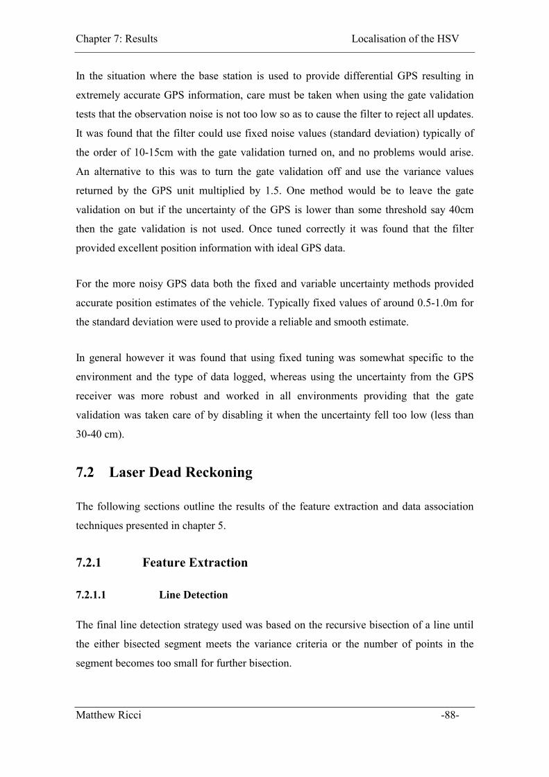
Chapter 7: Results Localisation of the HSV
In the situation where the base station is used to provide differential GPS resulting in
extremely accurate GPS information, care must be taken when using the gate validation
tests that the observation noise is not too low so as to cause the filter to reject all updates.
It was found that the filter could use fixed noise values (standard deviation) typically of
the order of 10-15cm with the gate validation turned on, and no problems would arise.
An alternative to this was to turn the gate validation off and use the variance values
returned by the GPS unit multiplied by 1.5. One method would be to leave the gate
validation on but if the uncertainty of the GPS is lower than some threshold say 40cm
then the gate validation is not used. Once tuned correctly it was found that the filter
provided excellent position information with ideal GPS data.
For the more noisy GPS data both the fixed and variable uncertainty methods provided
accurate position estimates of the vehicle. Typically fixed values of around 0.5-1.0m for
the standard deviation were used to provide a reliable and smooth estimate.
In general however it was found that using fixed tuning was somewhat specific to the
environment and the type of data logged, whereas using the uncertainty from the GPS
receiver was more robust and worked in all environments providing that the gate
validation was taken care of by disabling it when the uncertainty fell too low (less than
30-40 cm).
7.2 Laser Dead Reckoning
The following sections outline the results of the feature extraction and data association
techniques presented in chapter 5.
7.2.1 Feature Extraction
7.2.1.1 Line Detection
The final line detection strategy used was based on the recursive bisection of a line until
the either bisected segment meets the variance criteria or the number of points in the
segment becomes too small for further bisection.
Matthew Ricci -88-
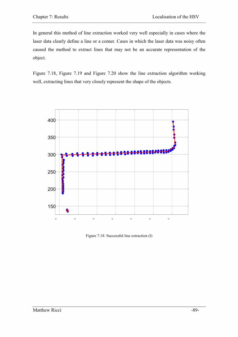
Chapter 7: Results Localisation of the HSV
In general this method of line extraction worked very well especially in cases where the
laser data clearly define a line or a corner. Cases in which the laser data was noisy often
caused the method to extract lines that may not be an accurate representation of the
object.
Figure 7.18, Figure 7.19 and Figure 7.20 show the line extraction algorithm working
well, extracting lines that very closely represent the shape of the objects.
- - - - - - -
150
200
250
300
350
400
Figure 7.18: Successful line extraction (I)
Matthew Ricci -89-
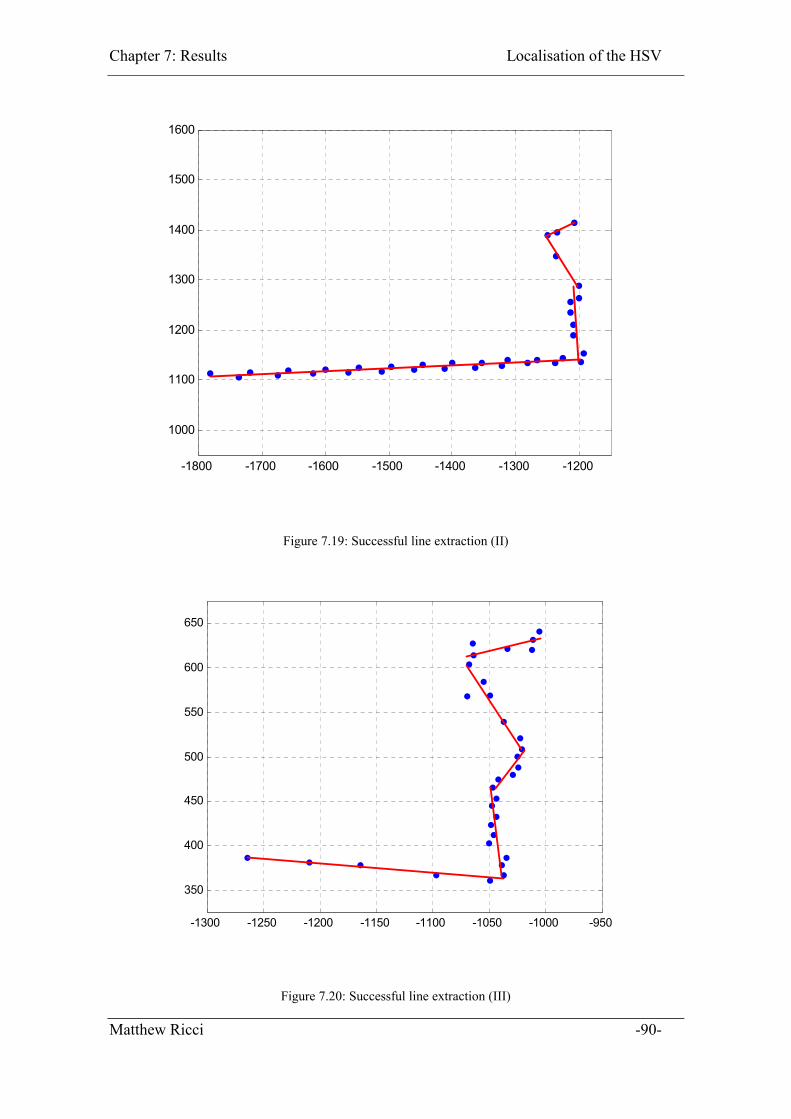
Chapter 7: Results Localisation of the HSV
-1800 -1700 -1600 -1500 -1400 -1300 -1200
1000
1100
1200
1300
1400
1500
1600
Figure 7.19: Successful line extraction (II)
-1300 -1250 -1200 -1150 -1100 -1050 -1000 -950
350
400
450
500
550
600
650
Figure 7.20: Successful line extraction (III)
Matthew Ricci -90-
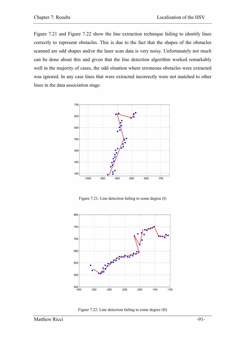
Chapter 7: Results Localisation of the HSV
Figure 7.21 and Figure 7.22 show the line extraction technique failing to identify lines
correctly to represent obstacles. This is due to the fact that the shapes of the obstacles
scanned are odd shapes and/or the laser scan data is very noisy. Unfortunately not much
can be done about this and given that the line detection algorithm worked remarkably
well in the majority of cases, the odd situation where erroneous obstacles were extracted
was ignored. In any case lines that were extracted incorrectly were not matched to other
lines in the data association stage.
-1000 -950 -900 -850 -800 -750
400
450
500
550
600
650
700
Figure 7.21: Line detection failing to some degree (I)
-400 -350 -300 -250 -200 -150 -100500
550
600
650
700
750
800
Figure 7.22: Line detection failing to some degree (II)
Matthew Ricci -91-
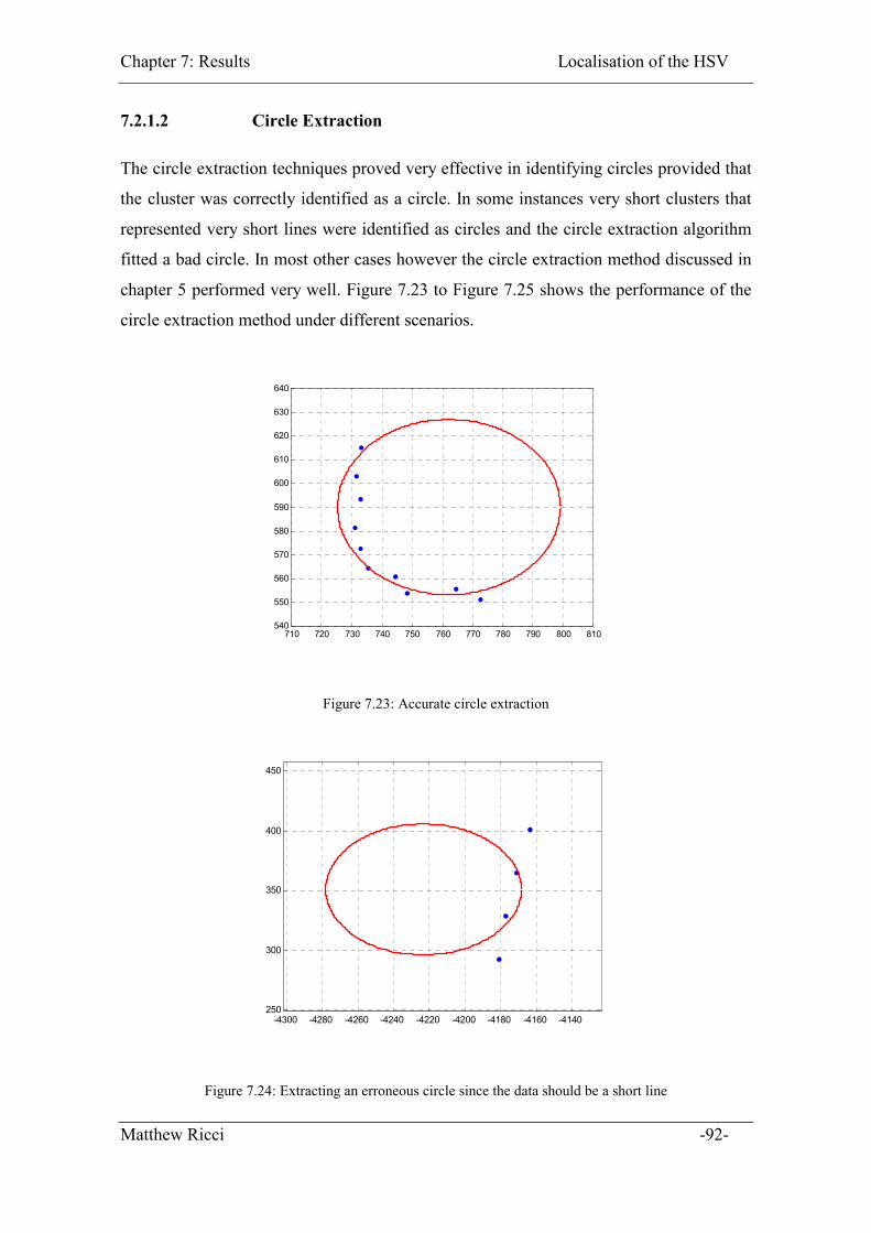
Chapter 7: Results Localisation of the HSV
7.2.1.2 Circle Extraction
The circle extraction techniques proved very effective in identifying circles provided that
the cluster was correctly identified as a circle. In some instances very short clusters that
represented very short lines were identified as circles and the circle extraction algorithm
fitted a bad circle. In most other cases however the circle extraction method discussed in
chapter 5 performed very well. Figure 7.23 to Figure 7.25 shows the performance of the
circle extraction method under different scenarios.
710 720 730 740 750 760 770 780 790 800 810540
550
560
570
580
590
600
610
620
630
640
Figure 7.23: Accurate circle extraction
-4300 -4280 -4260 -4240 -4220 -4200 -4180 -4160 -4140250
300
350
400
450
Figure 7.24: Extracting an erroneous circle since the data should be a short line
Matthew Ricci -92-
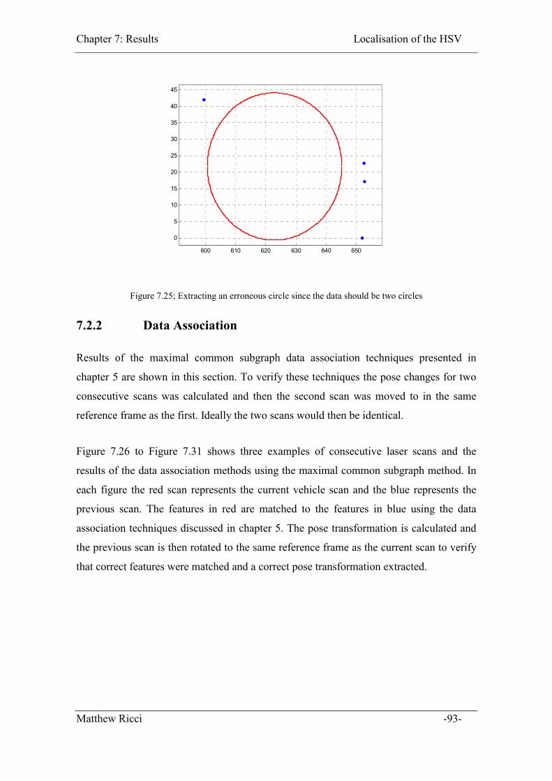
Chapter 7: Results Localisation of the HSV
600 610 620 630 640 650
0
5
10
15
20
25
30
35
40
45
Figure 7.25; Extracting an erroneous circle since the data should be two circles
7.2.2 Data Association
Results of the maximal common subgraph data association techniques presented in
chapter 5 are shown in this section. To verify these techniques the pose changes for two
consecutive scans was calculated and then the second scan was moved to in the same
reference frame as the first. Ideally the two scans would then be identical.
Figure 7.26 to Figure 7.31 shows three examples of consecutive laser scans and the
results of the data association methods using the maximal common subgraph method. In
each figure the red scan represents the current vehicle scan and the blue represents the
previous scan. The features in red are matched to the features in blue using the data
association techniques discussed in chapter 5. The pose transformation is calculated and
the previous scan is then rotated to the same reference frame as the current scan to verify
that correct features were matched and a correct pose transformation extracted.
Matthew Ricci -93-
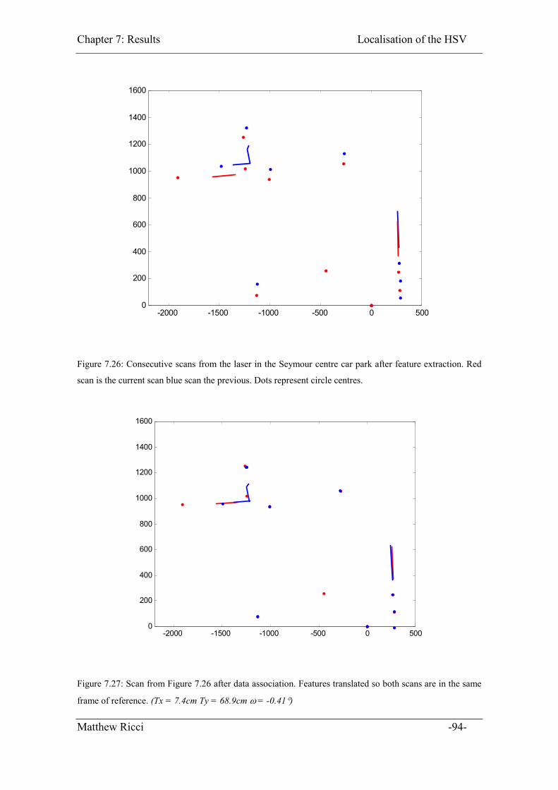
Chapter 7: Results Localisation of the HSV
-2000 -1500 -1000 -500 0 5000
200
400
600
800
1000
1200
1400
1600
Figure 7.26: Consecutive scans from the laser in the Seymour centre car park after feature extraction. Red
scan is the current scan blue scan the previous. Dots represent circle centres.
-2000 -1500 -1000 -500 0 5000
200
400
600
800
1000
1200
1400
1600
Figure 7.27: Scan from Figure 7.26 after data association. Features translated so both scans are in the same
frame of reference. (Tx = 7.4cm Ty = 68.9cm � = -0.41�)
Matthew Ricci -94-
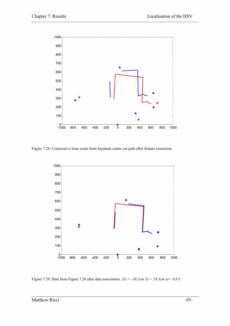
Chapter 7: Results Localisation of the HSV
-1000 -800 -600 -400 -200 0 200 400 600 800 10000
100
200
300
400
500
600
700
800
900
1000
Figure 7.28: Consecutive laser scans from Seymour centre car park after feature extraction.
-1000 -800 -600 -400 -200 0 200 400 600 800 10000
100
200
300
400
500
600
700
800
900
1000
Figure 7.29: Data from Figure 7.28 after data association. (Tx = -39.2cm Ty = 28.3cm � = 6.6�)
Matthew Ricci -95-
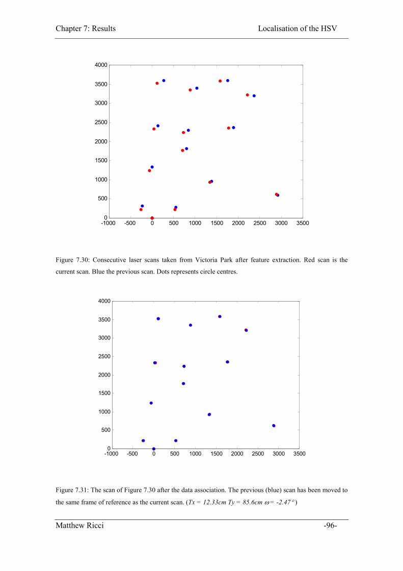
Chapter 7: Results Localisation of the HSV
-1000 -500 0 500 1000 1500 2000 2500 3000 35000
500
1000
1500
2000
2500
3000
3500
4000
Figure 7.30: Consecutive laser scans taken from Victoria Park after feature extraction. Red scan is the
current scan. Blue the previous scan. Dots represents circle centres.
-1000 -500 0 500 1000 1500 2000 2500 3000 35000
500
1000
1500
2000
2500
3000
3500
4000
Figure 7.31: The scan of Figure 7.30 after the data association. The previous (blue) scan has been moved to
the same frame of reference as the current scan. (Tx = 12.33cm Ty = 85.6cm � = -2.47� )
Matthew Ricci -96-

Chapter 7: Results Localisation of the HSV
The results indicate that the maximal common subgraph method for data association is
quite effective in determining a one to one matching of features between consecutive
scans and hence the pose change of the vehicle based on this information.
These pose changes were then summed and converted to the navigation coordinate frame
in an attempt to build up a path estimate of vehicle motion. Figure 7.32 shows the path
estimate built up from consecutive laser scans using the data set taken from the Seymour
centre car park (Figure 7.4 shows the actual path taken). Only the initial stages of the
dead reckoning are shown since after this the path estimates become somewhat
unreliable.
Figure 7.32: Laser Dead reckoning. Data set from seymour centre car park.
7.2.3 Summary
The techniques for data association and feature extraction presented here were quite
effective in the sense that the feature extraction process reliably identified the correct
features ion the majority of cases and the maximal common subgraph data association
technique provided the correct feature mapping in the vast majority of cases.
Estimating the pose change from this feature matching information proved quite effective
on an individual basis, i.e. simply matching two scans together. As can be seen from the
Matthew Ricci -97-

Chapter 7: Results Localisation of the HSV
results the error was small when two scans were mapped onto one another. However
when several feature mappings were strung together to form a path estimate of the
vehicle the data became unreliable since all the small errors present just grew with time.
As a consequence the laser dead reckoning path grew less and less accurate with time. As
was to be expected since this was a dead reckoning path of the vehicle with no absolute
information about the actual position.
It was hoped that the laser could be used as an alternative to the model for dead
reckoning in situations where the GPS dropped out for extended periods of time. It was
found that the laser dead reckoning was quite unpredictable and its performance could
not be guaranteed reliably for all data sets. Also due to the time constraints of this thesis,
the method was unable to be fine-tuned to produce a more robust algorithm.
Despite the relative failure of the using the laser to perform robust dead reckoning
predictions effective feature extraction and data association techniques were
implemented that could find many uses outside the scope of this thesis in areas of
mapping and reactive control.
Matthew Ricci -98-
Chapter 8:
Conclusion
The kalman filter presented in this thesis to fuse vehicle state prediction based on
encoder and LVDT data with GPS data performed reliably well in a number of different
scenarios. A suitable filter tuning was to provide accurate position estimates when using
the cm accuracy provided by the DGPS. Filter tuning was also provided to deal with the
much less accurate GPS data when not using DGPS. Multipath was a common problem
and testing showed that the filter was able to handle reasonable multipathed data. The
online performance of the filter verified the testing performed on the offline simulation.
The ideal situation for the filter is a wide-open area with no trees or even a sparse
covering of trees. The area must be relatively flat however since the navigation loop only
gives position data in 2 dimensions. If hilly areas are involved then alternate strategies
must be used such as an inertial system. Although the filter can handle the odd
occurrence of corrupt GPS data, the filter still requires that on the whole the GPS
information be good. Most importantly it is necessary to start the filter in an area where
the GPS information is known to be accurate.
The feature extraction techniques implemented in this thesis proved to be very accurate
in extracting features from raw laser data and even in these case where the features were
not extracted entirely correctly the problem was not continued by the data association
process.
Matthew Ricci -99-

Chapter 8: Conclusion Localisation of the HSV
The data association method implemented using a maximal common subgraph method to
find the one to one feature mapping between scans was very effective in mapping
features between consecutive scans. Initially it was postulated that laser based dead
reckoning may provide a more accurate dead reckoning procedure since it is non model
based. However the method proved to be often erratic if the correct number of feature
were not matched between scans to compute a valid pose transformation.
Although the laser dead reckoning was somewhat inaccurate the data association method
used could have many other potential applications such as tracking features in slam or in
map building and exploration strategies.
Future work may include developing a three dimension navigation loop using an inertial
unit, or using the navigation loop developed as an input to various control modules such
as path following.
Matthew Ricci -100-
Chapter 9:
Bibliography
[1] Bailey T., Nebot E., Rosenblatt J., Durrant-Whyte H., “Data Association and mobile
Robot Navigation: A Graph Theoretic Approach”, ICRA 2000, SF, USA, April 2000
[2] Barton M, "Controller Development and Implementation for Path Planning and
Following in an Autonomous Urban Vehicle". University of Sydney, Undergraduate
Thesis 2001
[3] Besl PJ, McKay HD, “A method for registration of 3-D shapes”, IEEE Transactions
on pattern analysis and machine intelligence, vol 14 issue 2, Feb 1992, pgs 239-256.
[4] Bomze, IM, Budinich M, Pardalos PM, and Pelillo M, “The maximal clique
problem”, Handbook of Combinatorial optimization (supplement volume A)m in D-
Z Du and P.M. Pardalos (eds.) Kluwer academic publishers, Boston, MA, 1999
[5] Bron C., Kerbosch J., “Algorithm 457 – Finding all cliques of an undirected graph”,
Communications of the ACM, vol 16, pp 575-577, 1973.
[6] Deitel H, Deitel P, “C: How to program”, Prentice Hall 1994.
[7] Farrel J., Barth M., “The Global Positioning System and Inertial Navigation”,
McGraw Hill, 1999
Matthew Ricci -101-
Chapter 9: Bibliography Localisation of the HSV
[8] Fitzgibbon T., "Remote Graphical User Interface for High Speed Vehicle" University
of Sydney, Undergraduate Thesis 1999
[9] Givant J, Baiker S, Nebot E, “Localisation and map building using laser range
sensors in outdoor applications” Journal of robotic systems 17(10), pg 565-583,
2000
[10] Isikyildiz G "The Hardware and Software Link Drivers for HSV" University of
Sydney, Undergraduate Thesis 1999
[11] Lee K, “Reactive Navigation for an autonomous outdoor vehicle”, thesis
undergraduate university of Sydney 2001.
[12] Lu F., Milios E., “Robot Pose estimation in unknown environments by matching 2D
range scans”, Proc. IEEE Comp. Soc. Conf. On computer vision and pattern
recognition, Seattle, WA (June 1994)
[13] Mallet A., "A specification of generic robotics software components: future
evolutions of GenM in orocos context" LAAS-CNRS, to be presented at ICRA 2002
[14] Mallet L, "Autonomous Rover Navigation on Unknown Terrains Functions and
Integrations" LAAS, To be published in International Journal of Robotics.
[15] McGregor J. J., “Backtrack Search Algorithms and the maximal complete subgraph
problem”, Software – Practice and Experience, vol 12, pp23-34, 1982
[16] Nebot E., Bailey T., Guivant J,. “Navigation Algorithms for autonomouse machines
in off road applications” Journal of autonomous robots. Downloaded off the www at:
www.acfr.usyd.edu.au
[17] Nebot E., Scheding S., “Navigation System Design”, Course notes for Navigation
Systems Design (KC-4) ACFR, March 27 2001 version 0.1
Matthew Ricci -102-
[18] Selvanathan A., “Australian Business Statistics”, South Melbourne, Vic. Nelson,
2000, 2nd ed.
Chapter 9: Bibliography Localisation of the HSV
[19] ShouryA., Aboutabl M., “Neural Network approach for solving the maximal common
subgraph problem” IEEE Transactions on systems, man and cybernetics, vol 26, no.
5, pp 785-790, 1996
[20] Sukkarieh S, Nebot EM, Durrant-Whyte H, “Achieving integrity in INS/GPS
Navigation loops for autonomous land vehicle applications”, proceeding of the 1998
IEEE international conference on Robotics and Automation, Leuven Belgium 1998.
[21] Sukkarieh S., “Introductory Estimation and the Kalman filter”, Mech 4701 Modern
estimation and control lecture notes 2002.
[22] Sukkarieh S., Nebot E.M, and Durrant-Whyte H.F., “A high integrity IMU GPS
navigation loop for autonomous land vehicle applications”, IEEE Transactions on
Robotics & Automation, vol 15, no. 3, Jun 1999 pg 572-578
[23] Van Wyk, C.J., “Data Structures and C programs” Reading, Mass: Adison Westley,
1988
[24] Welch G, Bishop G, “An introduction to the Kalman filter”, Department of computer
science, University of North Carolina at Chapel Hill. Downloaded of the www at:
http://www.cs.unc.edu/~welch/kalman/
[25] William H., “Numerical Recipes in C” Cambridge university press 1988, New York.
Matthew Ricci -103-

Abbreviations
DGPS – Differential Global Positioning System
GPS – Global Positioning System
HSV – High Speed Vehicle
IMU – Inertial Measurement Unit
LVDT – Linear variable displacement transducer
SLAM – Simultaneous Localisation and Mapping
ICP – Iterative Closest Point
IMRP – Iterative Matching Range Point
IDC – Iterative Dual Correspondence
ECEF – Earth Centred Earth Frame
NED – North East Down
GUI – Graphical User Interface
QNX – A real time operating system
MFC – Microsoft Foundation Class
Matthew Ricci -104-
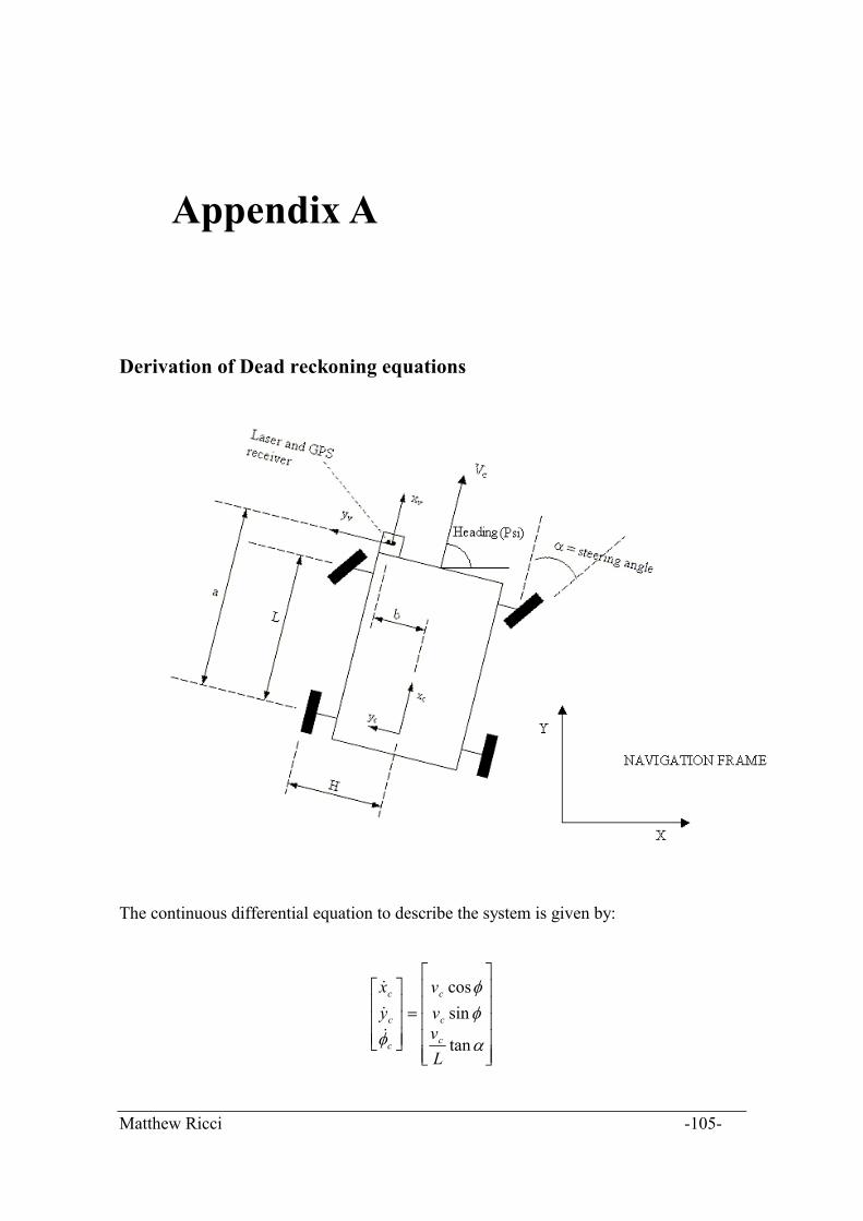
Appendix A
Derivation of Dead reckoning equations
The continuous differential equation to describe the system is given by:
�����
�
�
�����
�
�
�
���
�
�
���
�
�
�
�
�
� tan
sincos
Lvvv
yx
c
c
c
c
c
c
�
�
�
Matthew Ricci -105-

Appendix A Localisation of the HSV
Where:
vc is the velocity at the centre of the rear axle
Since the velocity is measured at the location of the encoder (ve), rear left wheel, the
velocity must be moved to the centre of the rear axle (vc) using the following equations.
From simple geometry we can see the position of the centre of the rear axle (PCx,PCy)
with respect to the wheel encoder (PEx, PEy) is:
�
�
cossin
HPPHPP
EyCy
ExCx
��
��
Differentiating this to get Vc gives:
��
��
sin
cos���
���
HPP
HPP
EyCy
ExCx
��
��
Given that and Y and )cos(�cCxc vvX ��� )sin(�cCyc vv ��
� �tan�Lvc
�� , the above
equations reduce to:
��
���
��
�
)tan(1 �
LH
vv e
c
The translation from the centre of the rear axle to the GPS antenna is given by:
��
��
cossinsincos
bayybaxx
cv
cv
���
���
Differentiating this gives:
����
����
sincos
cossin����
����
bayy
baxx
cv
cv
���
���
Matthew Ricci -106-

Appendix A Localisation of the HSV
Combining this with the original differential equations gives:
]sincos)[tan(sin
]cossin)[tan(cos
����
����
baLv
vy
baLv
vx
ccv
ccv
���
���
�
�
The discrete version of the above equation is:
� �
� �
���
����
����
tan)()1(
sincostansin)()1(
cossintancos)()1(
Lv
tkk
baLv
vtkYkY
baLv
vtkXkX
c
cc
cc
����
��
���
�����
��
���
�����
Where:
X is the ‘x’ position of the vehicle in the navigation frame
Y is the ‘y’ position of the vehicle in the navigation frame
� is the heading of the vehicle in the navigation frame
� is the current steering angle of the vehicle
�t is the sampling interval of the system (25ms in this thesis)
vc is the velocity at the centre of the rear wheels
L is the wheelbase of the HSV
a is the distance between the rear axle and the GPS receiver
b is the distance between the centreline of the vehicle and the GPS receiver
Matthew Ricci -107-

Appendix B
Closed-form Solution for Point Based Matching
For n pairs of points: a distance function between the
transformed P’s and the P
,,...,1),,(),,( /// niyxPyxP iiii �
/’s is defined as the following:
� ��
�
�
�
��������
���
n
iiyiiixiidist
n
idist
yTyxxTyxTE
PTPRTE
1
2/2/
1
2/
)cossin()sincos(),(
||),(
�����
��
By minimizing Edist we can obtain a closed form solution for Tx, Ty, and � as given
below:
)cossin(
)sincos(
arctan
/
/
//
//
��
��
�
yxyT
yxxT
SS
SS
y
x
yyxx
yxxy
���
���
�
�
�
where:
Matthew Ricci -108-

Appendix B Localisation of the HSV
��
��
��
��
��
��
��
��
������
������
��
��
n
iiiyx
n
iiixy
n
iiiyy
n
iiixx
n
ii
n
ii
n
ii
n
ii
xxyySyyxxS
yyyySxxxxS
yn
yxn
x
yn
yxn
x
1
//
1
//
1
//
1
//
1
//
1
//
11
))(())((
))(())((
11
11
//
//
Note also the coordinate transform to move the 2nd scan to the same frame of reference as
the first is given by the equations below.
Let P1 be a point on scan 2 and P2 be the corresponding point on scan 1, i.e. they both
represent the same point in the world. The two points are related by:
TPRP �� 12�
where:
���
����
� ��
��
��
� cossinsincos
R is the rotation matrix
���
����
��
y
x
TT
T is the translation vector
Matthew Ricci -109-

Appendix C
Polar Line Equations
Given the equation of a line in the form the polar parameters can be
calculated as follows.
01 �� �� xy
Form a line, perpendicular to the line of interest, that intersects with the origin. In the
figure above this is a line connecting point P with the origin. The equation of this line is
given by:
xy1
1�
��
Matthew Ricci -110-

Appendix C Localisation of the HSV
Point P(XP,YP) is given by the simultaneous solution of the two line equations
xy1
1�
�� & 01 �� �� xy
21
01
1 �
��
�
��Px
01 �� �� PP xy
Having found the coordinate of point P the polar line parameters are simply given by
simple trigonometry.
��
�
cos),(atan2
0�
�
rxy PP
The above equations apply for a regression from y to x. For regression from x to y simply
reverse xp and yp.
Matthew Ricci -111-

Appendix D
Finding all cliques of an undirected graph
The algorithm for finding all cliques of an undirected graph is presented in Bron &
Kerbosch [5] and is outlined in this appendix. For more details consult Bron and
Kerbosch.
The input graph is in the form of a symmetrical (m * m) matrix where m is the number of
nodes in the graph. A 1 in entry (i,j) indicates that node i and node j are connected. The
diagonal entries must all be 1.
The recursive algorithm is outlined below where the set CompSub indicates all possible
nodes for the current clique, the set candidates indicates all points that may in time serve
as extensions to CompSub and the set Not indicates all nodes that cannot be part of the
current clique.
Global integer N Comment: Size of the graph, number of nodes Global integer c
Comment: The input graph, with N nodes, in the form of a connection matrix Connected Global boolean Matrix: Connected[N][N] Global integer Array: CompSub[N]
Matthew Ricci -112-

Appendix D Localisation of the HSV
Function FindMaxClique() integer Array ALL[1:N] integer i
For i=1, step until i=N do ALL[i] = i end for
c = 0
ExtendVersion2(ALL, 0, N)
End FindMaxClique
Comment: ExtendVersion2 is recursive the function to find all cliques of the graph Connected.
Function ExtendVersion2(integer Array Old, integer ne, integer ce) integer Array new[1:ce] integer nod, fixp, newne, newce, i, j, count, pos, p, s, sel, integer minnod
minnod = ce; nod = 0
for i = 1 while i <= ce and minnod != 0 do p = old[i]; count = 0; j = ne;
Matthew Ricci -113-

Appendix D Localisation of the HSV
for j=j+1 while j <= ce and count < minnod do if connected[p,old[j]] == 0 then count = count +1 pos = j end if end for
if count < minnod then fixp = p; minnod = count if i <= ne then s = pos else s = 1; nod = 1; end if end if end for
for nod = minnod + nod step –1 until nod = 1 do p = old[s]; old[s] = old[ne+1]; sel = p; old[ne+1] = p; newne = 0;
for I = 1 while I <= ne step 1 do if connected[sel, old[I]] == 1 then newne = newne+1; new[newne] = old[I] end if end for
newce = newne;
for I = ne+1 while I <= ce step 1 do if connected[sel,old[I] == 1 then newce = newce+1;l new[newce] = old[I] end if end for
Matthew Ricci -114-

Appendix D Localisation of the HSV
Matthew Ricci -115-
c = c+1; compsub[c] = sel;
if newce == 0 then Comment: Compsub contains a clique, save this clique to check later if this clique is the maximal clique else if newne < newce then ExtendVersion2(new, newne, newce) end if
c = c-1 ne = ne+1 if nod > 1 then s = ne; s = s+1; while Connected[fixp, old[s]] == 0 do s = s+1 end while end if end for
end ExtendVersion2