NBER WORKING PAPER SERIES

NEIGHBORHOOD EFFECTS ON CRIMEFOR FEMALE AND MALE YOUTH:

EVIDENCE FROM A RANDOMIZED HOUSING VOUCHER EXPERIMENT

Jeffrey R. KlingJens Ludwig

Lawrence F. Katz

Working Paper 10777http://www.nber.org/papers/w10777

NATIONAL BUREAU OF ECONOMIC RESEARCH1050 Massachusetts Avenue

Cambridge, MA 02138September 2004

An earlier version of this paper was circulated as “Youth Criminal Behavior in the Moving To Opportunity Experiment,”Princeton IRS Working Paper 482, March 2004. Support for this research was provided by grants from the NationalScience Foundation to the National Bureau of Economic Research (9876337 and 0091854) and the National Consortiumon Violence Research (9513040), as well as by the U.S. Department of Housing and Urban Development, the NationalInstitute of Child Health and Human Development and the National Institute of Mental Health (R01-HD40404 and R01-HD40444), the Robert Wood Johnson Foundation, the Russell Sage Foundation, the Smith Richardson Foundation, theMacArthur Foundation, the W.T. Grant Foundation, and the Spencer Foundation. Additional support was provided bygrants to Princeton University from the Robert Wood Johnson Foundation and from NICHD (5P30-HD32030 for theOffice of Population Research), by the Princeton Industrial Relations Section, the Bendheim-Thoman Center forResearch on Child Wellbeing, the Princeton Center for Health and Wellbeing, the National Bureau of EconomicResearch, and a Brookings Institution fellowship supported by the Andrew W. Mellon foundation. We are grateful tonumerous colleagues for valuable suggestions, including: Todd Richardson and Mark Shroder at HUD; Judie Feins,Barbara Goodson, Robin Jacob, Stephen Kennedy, and Larry Orr of Abt Associates; our collaborators Jeanne Brooks-Gunn, Alessandra Del Conte Dickovick, Greg Duncan, Jane Garrison, Tama Leventhal, Jeffrey Liebman, MeghanMcNally, Lisa Sanbonmatsu, Justin Treloar and Eric Younger; seminar discussants Christopher Jencks, Dan O’Flahertyand Robert Sampson; Edward Glaeser and four referees; and seminar participants at Berkeley, the Homer Hoyt Institute,the Kennedy School, and the NBER. Any findings or conclusions expressed are those of the authors. The viewsexpressed herein are those of the author(s) and not necessarily those of the National Bureau of Economic Research.

©2004 by Jeffrey R. Kling, Jens Ludwig, and Lawrence F. Katz. All rights reserved. Short sections of text, not to exceedtwo paragraphs, may be quoted without explicit permission provided that full credit, including © notice, is given to thesource.

Neighborhood Effects on Crime for Female and Male Youth: Evidence from a RandomizedHousing Voucher ExperimentJeffrey R. Kling, Jens Ludwig, and Lawrence F. KatzNBER Working Paper No. 10777September 2004JEL No. H43, I18, J23

ABSTRACT

The Moving to Opportunity (MTO) demonstration assigned housing vouchers via random lottery to

public housing residents in five cities. We use the exogenous variation in residential locations

generated by MTO to estimate neighborhood effects on youth crime and delinquency. The offer to

relocate to lower-poverty areas reduces arrests among female youth for violent and property crimes,

relative to a control group. For males the offer to relocate reduces arrests for violent crime, at least

in the short run, but increases problem behaviors and property crime arrests. The gender difference

in treatment effects seems to reflect differences in how male and female youths from disadvantaged

backgrounds adapt and respond to similar new neighborhood environments.

Jeffrey R. KlingDepartment of Economicsand Woodrow Wilson SchoolPrinceton UniversityPrinceton, NJ 08544and NBERkling@princeton.edu

Jens LudwigPublic Policy InstituteGeorgetown University Washington, DC 20007ludwigj@georgetown.edu

Lawrence F. KatzDepartment of EconomicsHarvard UniversityCambridge, MA 02138and NBERlkatz@harvard.edu

1

I. INTRODUCTION

A growing theoretical literature predicts that the monetary and non-monetary returns to

criminal activity are likely to be greater in communities where crime and economic disadvantage

are more prevalent.1 Empirical tests of this hypothesis come primarily from relating the behavior

of individuals to the characteristics of the neighborhoods where they or their families have

selected to live.2 Most research suggests that disadvantaged neighborhoods are “criminogenic.”3

Yet drawing causal inferences from such findings is complicated by the possibility of

unmeasured individual- or family-level attributes that influence both criminal activity and

neighborhood selection. Predicting the magnitude or even direction of this bias is difficult.4

In this paper we overcome this basic identification problem by examining the effects of

neighborhood mobility on youth crime using data from the Moving to Opportunity (MTO)

randomized housing-mobility experiment. Sponsored by the U.S. Department of Housing and

Urban Development (HUD), MTO has been in operation since 1994 in five cities: Baltimore,

Boston, Chicago, Los Angeles, and New York. Eligibility for the program was restricted to low-

income families with children in these five cities, living within public or Section 8 project-based

1 Epidemic models emphasize the tendency of “like to beget like” through peer interactions with higher local crime rates serving to reduce the actual or perceived probability of arrest as well as the stigma of criminal behavior [Sah 1991; Cook and Goss 1996; Glaeser, Sacerdote, and Scheinkman 1996]. Collective socialization models focus on variation across neighborhoods in the ability or willingness of local adults to maintain social order [Wilson 1987; Sampson, Raudenbush, and Earls 1997]. Institutional models emphasize the roles of the quality or quantity of local schooling opportunities, police, and other institutions. In contrast, some theories suggest that moves to less disadvantaged communities may have little effect on crime, if for example teens simply rejoin the same types of peer groups as in their old neighborhoods [Jencks and Mayer, 1990]. Such moves could even increase criminal behavior if youth feel resentful towards or are discriminated against by their new, more affluent peers. 2 A different approach is taken by Glaeser, Sacerdote, and Scheinkman [1996], who show that observed variation in crime rates exceeds what can be predicted by “fundamental” factors. This excess variation is attributed to social interactions. 3 One recent review argues that of the outcomes studied in the neighborhood effects literature, the “strongest evidence links neighborhood processes to crime” [Sampson, Morenoff, and Gannon-Rowley 2002]. 4 Many social scientists believe that conditional on observed family characteristics, the more effective or motivated parents will be the ones who wind up in more-, rather than less-, advantaged communities. Yet the short-term results from the Boston and Baltimore sites of the Moving to Opportunity demonstration suggest that among parents assigned to the mobility treatment groups, those whose children are at relatively greater risk for problem or criminal behavior are the ones who are most likely to relocate through the program [Katz, Kling, and Liebman 2001; Ludwig, Duncan, and Hirschfield 2001].

2

housing in selected high-poverty census tracts.5 Around two-thirds of the roughly 4600 families

who volunteered for the program from 1994 to 1997 were African-American, while most of the

rest were Hispanic. Those families who signed up for MTO were randomly assigned into one of

the following three groups: experimental, Section 8, and control. The “experimental” group was

offered the opportunity to relocate using a housing voucher that could be used to lease a unit

only in census tracts with 1990 poverty rates of 10 percent or less.6 Families assigned to the

“Section 8” group were offered housing vouchers with no constraints on where the vouchers

could be redeemed. Families assigned to the “control” group were offered no services under

MTO, but did not lose access to social services to which they were otherwise entitled.

Because of random assignment, MTO yields three comparable groups of families living

in very different kinds of neighborhoods during the post-program period. Previous studies that

used the exogenous variation in neighborhoods induced by MTO within individual sites suggest

that moving to less distressed communities reduces anti-social behavior by youth in the short run

(one to three years after random assignment) in the Baltimore and Boston sites, but not in the

New York site.7 The present paper is the first to examine neighborhood effects on youth crime

using uniform outcome measures – both administrative arrest records and follow-up surveys –

from all five MTO sites. For MTO youth 15-25 at the end of 2001 we have from 4 to 7 years of

5 Section 8 project-based housing might be thought of as privately-operated public housing [Olsen 2003]. HUD contracts with private providers to develop and manage projects that include units reserved for low-income families. 6 Housing vouchers provide families with subsidies to live in private-market housing. The subsidy amount is typically defined as the difference between 30 percent of the household’s income and the HUD-defined Fair Market Rent, which equals either the 40th or 45th percentile of the local area rent distribution. MTO experimental group families were also provided with mobility assistance and in some cases other counseling services. Movers through MTO in the experimental group were required to stay in low-poverty tracts for a year to retain their vouchers. 7 In the Boston site, boys in the experimental and Section 8 groups exhibit about one-third fewer problem behaviors compared to controls in the short run [Katz, Kling, and Liebman 2001]. For the Baltimore site, official arrest data suggest that teens in both treatment groups are less likely than controls to be arrested for violent crimes. These short-run impacts are large for both boys and girls, but not statistically significant when disaggregated by gender [Ludwig, Duncan, and Hirschfield 2001]. Short-term survey data from the New York site reveals no statistically significant differences across groups in teen delinquency or substance use [Leventhal and Brooks-Gunn 2003].

3

post-randomization data, with an average of 5.7 years. Our surveys also provide data on youth

and neighborhood attributes that current theories predict should mediate neighborhood effects.

Our main finding is that moving to a lower-poverty, lower-crime neighborhoods produces

different effects on the criminal behavior of male versus female youth. Through the first two

years after random assignment, the offer of a housing voucher affected youth criminal behavior

in the direction predicted by prevalent theories of social interactions: both male and female

youth in the experimental group experience fewer violent-crime arrests compared to those in the

control group, and females are also arrested less often for other crimes as well. However, several

years after random assignment the treatment effects for male and female youth diverge in a way

not easily captured by the standard theories for neighborhood effects. Although the beneficial

effects on most crime types persist for female youth, property crime arrests become more

common for experimental than control group males.8

These gender differences in estimated neighborhood effects for crime – also found in

recent MTO research on mental and physical health, education, and substance use [Kling and

Liebman 2004] – echo the gender differences observed in national data for U.S. blacks in several

domains. Black males have lower achievement test scores than either white males or black

females, and black-white differences in wages and annual earnings continue to be more

pronounced for males than females, even after controlling for pre-market skills [Neal and

Johnson, 1996; Johnson and Neal, 1998]. Trends in criminal activity also reveal pronounced

gender differences as seen in Figure 1, which shows homicide offending rates for black males

and females ages 18-24 for the period covering 1976 to 2000. Setting aside the volatility in the

8 The increase in property-crime arrests for experimental-group males may be partially explained by an increase in the probability of arrest in lower-poverty communities, but support for the idea that this represents a real effect on criminal behavior comes from our finding of a positive experimental-control difference for males in self-reported problem behaviors as well.

4

series for black males, which is due in part to changes in violence associated with drug markets9,

the homicide offending rate was about 25 percent higher in 2000 than in 1976. In contrast, the

homicide offending rates for black females declined by nearly two-thirds over this period.10 Life

expectancy trends show a similar gender gap for blacks with the (age-adjusted) all-cause

mortality rate having declined by 41% from 1960 to 1998 for black females as opposed to only

29% for black males.11 The findings on gender differences in neighborhood effects from MTO

suggest that reductions in the racial and economic residential segregation as well as other

improvements in economic opportunities and educational access may have more beneficial

effects for black females than black males.12

The difference in neighborhood effects observed in the MTO data seems to reflect

differences in how males and females respond to similar neighborhoods. We find that boys and

girls in the same treatment groups move into similar types of neighborhoods, and within families,

brothers and sisters respond differentially to the same mobility patterns. One candidate

explanation for why boys and girls respond differently to the same neighborhoods is greater

discrimination against minority males. Yet any discrimination experienced by MTO youth is

more likely to be due to social class rather than race, given that MTO moves produce

surprisingly modest changes in racial integration and no changes in youths’ experiences with

racial discrimination. An alternative explanation is gender differences in adapting to change,

although this hypothesis does not seem consistent with the short-term reduction in violent-crime

9 See Cook and Laub [1998], Blumstein and Wallman [2000], and Levitt [2004]. 10 For blacks 14-17 homicide offending rates were volatile over this period for both males and females, although show a net decline in 2000 versus 1976 for females but not for males. For blacks 25 and over offending rates declined steadily from 1976-2000 for both genders; however the decline was larger for females than males (79% versus 60%). The patterns for white males versus females are qualitatively similar; for more details, see Fox and Zawitz [2002]. 11 See Table 9 in Haines [2002]. By comparison, for whites there was very little gender difference in the decline in death rates over this period (38% for males and 36% for females). 12 See Cutler, Glaeser and Vigdor [1999] and Glaeser and Vigdor [2001] for trends in residential racial segregation, and see Watson [2003] and Massey and Fischer [2003] for trends in residential economic segregation.

5

arrests for experimental boys or with the fact that the increase in property-crime arrests for this

group shows up only several years after random assignment. In our view the most likely

explanation is that boys are more likely than girls to have or take advantage of a comparative

advantage in property offending in their new neighborhoods. This possibility provides an

explanation for the delayed increase in property crime arrests for male youth in the experimental

versus control groups – it may take time for boys to learn about this comparative advantage.

The remainder of the paper is organized as follows. Section II describes our data and

econometric approach. Section III presents our main findings for neighborhood effects on crime

and delinquency by male and female youth. We explore possible explanations for the gender

difference in treatment effects in section IV, while section V concludes.

II. DATA AND ANALYTICAL METHODS

A. Data

Our data on youth delinquency and criminal behavior are derived from two main sources:

administrative arrest records and survey data. Information on potential mediating processes

comes from our surveys, as well as administrative data on local-area crime rates measured at the

level of either the police beat (for urban residents) or municipality or county (for suburban

residents). These data sources are described in detail in Appendix A.

Our main analytic sample consists of MTO youth 15-25 at the end of 2001, which

captures the set of MTO participants that have spent at least part of their peak criminal-offending

ages during the post-program period.13 Our arrest records capture youth criminal behavior for

13 The administrative arrest records for our MTO sample show that annual arrest rates begin to increase noticeably around age 13 or 14, and peak between the ages of 18 and 20 among young adults in the control group (corresponding to those ages 22-25 at the end of 2001). The proportion ever arrested is more than 2.5 times higher for males than females (53 versus 19 percent). The “criminal careers” of the MTO control group appear to follow a trajectory that is similar to what has been found for other urban samples [Tracy, Wolfgang, and Figlio 1990].

6

this group through the end of 2001. The age at which youth are treated as adults by criminal

justice agencies is typically between 16 and 18, so we attempted to match MTO participants to

both adult and juvenile arrest records using information such as name, race, sex, date of birth,

and social security number. We obtained records from agencies in the states of the five MTO

sites as well as from 15 other states to which MTO participants had moved. Although some

youth moved to states from which we did not obtain administrative data, we have complete arrest

histories for 93 percent of youth and the response rate is very similar across MTO groups.

Our second source of data comes from surveys completed during 2002 with 1807 youth

ages 15-20 from the MTO households. The overall effective response rate for the survey is 88

percent and is somewhat higher for females than males (90 percent versus 86 percent), but quite

similar across MTO groups, equal to 87 percent for the experimental and control groups and 90

percent for the Section 8 group. The surveys were generally conducted in-person and captured

self-reported arrests as well as other delinquent and anti-social behaviors. Interviews were also

conducted separately with an adult (usually the youth’s mother) from the MTO household.

B. Descriptive statistics

At the time of enrollment, the head of household completed a baseline survey that

included information about the family as well as some specific information about each child.

Descriptive statistics for the baseline characteristics of youth in our main administrative data

sample (ages 15-25 at the end of 2001) and our survey sample (ages 15-20 at the end of 2001)

are shown in Table I. None of the treatment-control differences for any characteristic for either

sample is statistically significant at the .05 level.

Eligibility for the MTO program was limited to families in public housing or Section 8

project-based housing located in some of the most disadvantaged census tracts in the five MTO

7

cities and, for that matter, in the country as a whole. Of the families with youth 15-25 at the end

of 2001, 41 percent of those in the experimental group and 55 percent of those in the Section 8

group relocated through MTO.14 These moves led to substantial differences across treatment

groups in census tract characteristics, although these differences narrow somewhat over time due

to the subsequent mobility of the treatment and control families, as seen in Table II. The final

panel of Table II shows that parents of youth 15-25 assigned to the experimental group are less

likely than control-group parents to report that their neighbors would do nothing about truant

youth or graffiti, two common measures of local social organization and order maintenance

[Sampson, Raudenbush, and Earls 1997]. Parents in the experimental group are also less likely

than controls to report that they have trouble with police not coming when called. The

differences in survey reports between the Section 8 and control groups are less pronounced.

C. Analytical methods

In principle one could use the exogenous variation in neighborhood conditions generated

by MTO to estimate the effects of specific census tract characteristics on youth crime. However

Table II shows that in practice MTO changes a variety of neighborhood attributes for program

participants. With only two MTO treatment groups, disentangling the effects of specific

neighborhood characteristics on youth behavior will be difficult.

In our analysis we instead focus on identifying the causal effects of the MTO treatment

itself, which provides a reduced-form estimate for the net effect of the constellation of

neighborhood changes induced by the program. Our main findings come from simply comparing

the average outcomes of youth assigned to different MTO groups, known as the intent-to-treat

(ITT) effect, which identifies the causal effect of offering families the services made available

14 The take-up rates are quite similar for our youth survey sample (ages 15-20), equal to 44 and 57 percent for the experimental and Section 8 groups, respectively.

8

through the experimental or Section 8 treatments. Let Y represent an outcome of interest. We

estimate a model using pooled data from all three MTO groups with Z consisting of two separate

indicators for assignment to the experimental and Section 8 groups. We calculate the ITT effects

as the two elements of π1 in equation (1) using ordinary least squares, conditioning on a set of

(pre-random assignment) baseline characteristics (X), where i indexes individuals.15

(1) Yi = Ziπ1 + Xi�1 + �1i

Standard errors are adjusted for the presence of youth from the same family. These and all other

estimates in this paper are computed using sample weights.16

To examine whether treatment effects vary by gender, we estimate a modified version of

equation (1) that includes interactions between indicators for treatment group and gender,

denoted by the indicator G which is one for females. G is also included as an element of X.

(2) Yi = (1-Gi)Ziπ20 + GiZiπ21 + Xi�2 + �2i

In equation (2), the difference in average outcomes between the males in the treatment and

control groups is represented by π20 and for females the difference is represented by π21.

To understand the effects of actually changing neighborhoods, we also present separate

estimates for the effects of treatment on the treated (TOT). In our application, the “treatment” is

15 These include site, survey measures of the socio-demographic characteristics of household members, and survey reports about youth experiences in school such as expulsions or enrollment in gifted and talented classes. In models where the outcome of interest comes from official arrest data, we also condition on a set of indicators for the number of pre-program arrests for violent, property, drug or other offenses. The complete list of covariates is given in Appendix Table A1. Because the distribution of pre-program characteristics should be balanced across treatment groups with random assignment, conditioning on these variables serves mainly to improve the precision of the treatment effect estimates. 16 The weights we use to analyze survey-reported outcomes have three components, described in detail in Orr et al. [2003], Appendix B. The survey procedure attempted to contact a subsample of difficult-to-locate cases. Sub-sample members receive greater weight since, in addition to themselves, they represent individuals whom we did not attempt to contact during the sub-sampling phase. Survey youth from large families receive greater weight since we randomly sampled two children per household so these youth represent a larger fraction of the study population. Weights are also used since the ratio of individuals randomly assigned to treatment groups was changed during the course of the demonstration to adjust in response to differences between projected and actual use of offered vouchers, and weighting avoids potential confounding of treatment group with calendar time effects. Individuals within treatment groups are weighted by their inverse probability of assignment to the group to account for changes in the random assignment ratios. Models for official arrest outcomes use only this last weighting component.

9

defined as relocation through the MTO program.17 The TOT estimate seeks to identify the effect

of moving through the MTO program compared to what these families would have experienced

otherwise. The TOT impact can be calculated as the ITT effect divided by the difference in

treatment take-up rates [Bloom 1984]. We use two-stage least squares with treatment group

assignment as the instrumental variable for treatment take-up.18

III. NEIGHBORHOOD EFFECTS ON YOUTH DELINQUENCY AND CRIME

To preview the findings in this section, our analysis suggests that moving to lower

poverty neighborhoods leads to fewer violent and property crime arrests for females, and fewer

violent but more property crime arrests for males. Compared to males in the control group, those

in the experimental group also have higher rates of self-reported problem behaviors.

Table III presents estimates of the effects of the MTO treatments on lifetime arrests

through 2001 based on administrative data for the overall sample of youth ages 15-25 (pooling

males and females).19 We find that assignment to the experimental group substantially reduces

the incidence of violent-crime arrests. The ITT effect of -.061 is equal to around 15 percent of

17 The control group experienced substantial mobility over our study period. Relative to the counterfactual experience of what would have happened if a family had been assigned to the control group, the MTO voucher “treatments” typically induced families to move earlier and to lower poverty neighborhoods. 18 Specifically, we estimate equations analogous to (1) and (2), but with an endogenous Z indicating treatment take-up, and with treatment assignment as excluded instruments. The TOT estimate will be an unbiased estimate of the effect of treatment on the treated if random assignment is truly random, and if assignment to the treatment group has no effect on those who do not move through MTO. This second assumption may not be literally true, since the counseling services and search assistance offered to treatment families may influence later mobility patterns or other youth behaviors even among families that do not relocate through MTO. The disappointment of searching but failing to find an apartment may also affect non-movers in the treatment groups. If the effects of treatment-group assignment are substantially smaller for those who do not move through MTO compared to those who do (although not exactly zero as assumed in TOT estimation), our TOT estimates will approximate the effects of MTO moves on those who move through the MTO program. 19 We focus on lifetime arrests because this is an intuitively more meaningful unit of measurement than post-random assignment arrests, and because this concept is used in the MTO youth survey. The survey asked about lifetime arrest experiences because youth were expected to have trouble determining which arrests occurred before rather than after random assignment. Results for differences between groups in lifetime arrests and post-randomization arrests are very similar, because the distribution of pre-program arrests is balanced across MTO groups. With our administrative data on lifetime arrests, we explicitly condition on each youth’s pre-program arrest history.

10

the control group’s mean number of lifetime arrests for violent crimes. The experimental-control

difference in total lifetime arrests for all types of crime is not statistically significant, largely

because of the positive (but insignificant) difference in property-crime arrests. The final two

columns of Table III show the effects of the Section 8 intervention, which is essentially like the

large-scale housing voucher program in operation throughout the country. The effects of moving

through the Section 8 treatment on violent-crime arrests is about one-third the TOT effect from

the experimental treatment and not statistically significant, consistent with the fact that the

neighborhood changes experienced by MTO movers are more pronounced in the experimental

than Section 8 group along almost every dimension (Table II). None of the Section 8-control

differences in arrests are statistically significant.

One lens through which to view these effects for different offense types is to compare the

lifetime social costs of criminal offending for youth across MTO groups, which we have

attempted to do by combining the cost-of-crime estimates presented in Miller, Cohen, and

Wiersema [1996] and the estimated program impacts on these disaggregated crime categories,

with details given in Appendix B. The experimental group has lower point estimates lifetime

costs of offending than the control group, with ITT effect sizes ranging from 15 to 33 percent of

the costs imposed by control-group youth (as seen in Appendix Table B1), although the effects

are not statistically significant. These social cost estimates should be interpreted with caution

given their imprecision and given inherent difficulties in measuring the costs of crime.

Table IV shows that the results for all youth mask important differences in treatment

effects by gender. As seen in Panel A, female youth assigned to the experimental group

experience about one-third fewer arrests for violent and property offenses compared to the

control group, and about one-third fewer arrests overall. For males the experimental effect on

violent crime arrests is smaller and is not significantly different from either zero or the treatment

11

effect for females. The most striking gender difference in program impacts is for property-crime

arrests, where the experimental treatment effect for males is positive and large, equal to nearly

one-third of the control group’s mean.20 Panel C shows that the Section 8 treatment effects on

arrests are generally similar in sign but muted compared to the experimental treatment. In terms

of lifetime costs of crime for youth ages 15-25, shown in Appendix B, our point estimates

indicate lower costs for both treatment groups relative to the control group across both genders.

The increase in property crime for experimental-group males is more than offset by the decrease

in violent crime arrests in terms of lifetime offending costs relative to the control group.

Because the MTO youth surveys are only available for program participants up to age 20

at the end of 2001, in panels B and D of Table IV we replicate some of the key administrative

data results for youth ages 15-20. The pattern of results for the total number of lifetime arrests is

qualitatively similar to those for our preferred youth sample ages 15-25. In analyses not shown

in the table, we find that the program impacts are not substantially different for those who were

in their early versus late adolescent years at the time of random assignment, and that interactions

of treatment effects with age are not significant.21

20 The estimated experimental effects on property-crime arrests for male youth suggest that the identifying assumption behind the TOT estimates may not strictly hold, at least for this outcome and group of program participants. With information about the experimental group take-up rate, the TOT effect, and the mean arrest rate for experimental group “compliers” and “non-compliers” – using the terminology of Angrist, Imbens, and Rubin [1996] – we can calculate the implied arrest rate among the control group compliers. The control complier mean (CCM), defined by Katz, Kling, and Liebman [2001], that is implied by the experimental effects on male property-crime arrests is .215. This is quite low relative to the CCM for Section 8 effects on male property crime, and also lower than the CCMs for female property crime. We do not believe that this is due to an unusually low property-crime arrest rate among control group boys, because this arrest rate is similar to what is observed for the MTO Section 8 group and for the set of male youth in public housing whose families applied to the city of Chicago’s housing voucher program [Ludwig et al. 2004]. Part of the explanation seems to be that the property-crime arrest rate among male youth in the experimental non-complier group is much higher than what is observed for the Section 8 non-compliers. The elevated property-crime arrest rate for male youth experimental non-compliers appears to be driven by those in families that started but did not complete the experimental treatment counseling program. 21 When the analysis of lifetime arrests by type of offense is limited to the sample of youth aged 15-20 in 2001, we find quite similar results to those for the full 15-25 age group. The main differences are that the property crime effect for experimental group females is negative but insignificant, and the effects for both treatment groups of males on arrests for “other” crimes are positive and significant for the sample restricted to youth aged 15-20.

12

We can also use our administrative data to examine neighborhood effects on the

likelihood of having ever been arrested, which is the arrest measure available with the MTO

youth surveys. For the experimental group the ITT and TOT effects on the number of lifetime

arrests are (as a proportion of the control mean) much larger than the effects on ever arrested,

suggesting that much of the beneficial effect for females and detrimental effect for males come

from neighborhood effects on the volume of arrests for those who are criminally involved. In

contrast to the results from the administrative records, data from survey self-reports of arrest

reveal no statistically significant treatment effects for either treatment group or gender, or any

significant differences between male and female youth in treatment effects. We believe that part

of the reason that we do not see statistically significant between-group differences in the survey

data is that MTO youth appear to under-report anti-social behavior to our interviewers.22

Although misreporting appears to be a problem with the self-reported survey data, the

administrative data results may be susceptible to bias from a different source, namely variation

across neighborhoods in the probability of arrest. Table II showed that parents in the two MTO

treatment groups are much less likely than those in the control group to report that the

neighborhood has a problem with police not coming when called. If parent reports about the

quality of local policing are positively related to the probability that a crime results in arrest, then

treatment effects on the probability of arrest will have two conflicting impacts on treatment-

control group differences in arrest rates. On one hand, more and better policing may deter

22 Direct evidence for under-reporting with our MTO survey measure of “ever arrested” comes from a comparison with the official arrest data for these same youth. The control mean for our survey measure equals about two-thirds of the figure recorded by official data. For females, the survey estimate is about one-half of the official one, and for males it is about three-quarters. However uniform under-reporting to the surveys by youth in all three MTO groups can explain only part of the difference between the results from the survey versus official arrest data. A data-generating model with a constant propensity to under-report arrests, orthogonal to treatment-group assignment, could explain the entire difference between the survey and administrative-data point estimates for the experimental treatment’s impact on females. But such a model could explain less than one-tenth of the difference in point estimates for the experimental-control contrast for males, and only around one-quarter and one-half of the difference in the Section 8-only point estimates for females and males, respectively.

13

criminal behavior, thereby leading to fewer arrests within the treatment group than control group.

On the other hand, setting deterrence aside, the mechanical relationship between the probability

of arrest (P), criminal behavior (C) and arrests (A), with P×C=A, would lead the treatment

groups to have higher arrest rates than controls even if there are no differences across groups in

criminal behavior. This latter relationship would lead us to understate treatment effects that

reduce youth crime and overstate treatment effects that increase youth crime. A policing

intensity bias would have to work in opposite directions for males and females to explain the

experimental treatment effects for both genders.

Some evidence that the experimental treatment effect on property-crime arrests for male

youth may represent a real behavioral effect rather than variation across areas in law enforcement

practices comes from the experimental-control difference in self-reported problem behaviors.

Panel B of Table IV shows that male youth assigned to the experimental group have an average

score on our behavior problems index that is nearly 20 percent higher than that of the control

group.23 We find no significant difference between experimental and control group males on a

delinquency index directly measuring theft and other more serious anti-social behaviors.24

Finally, Table V shows the dynamics of treatment impacts on arrest rates for youth ages

15-25, where the units are arrests per person per year as opposed to the number of lifetime arrests

as in Tables III and IV.25 During the first two years following random assignment, males in the

23 The behavior problems index is defined as the fraction of 11 problems that youth report to be “often” or “sometimes” true of themselves: has difficulty concentrating; cheats or lies; teases others; is disobedient at home; has difficulty getting along with other children; has trouble sitting still; has a hot temper; would rather be alone; hangs around other children who get into trouble; is disobedient at school; has trouble getting along with teachers. 24 The delinquency index is defined as the fraction of nine activities in which youth report they have ever engaged: carrying a hand gun; belonging to a gang; damaging property; stealing something worth less than $50; stealing something worth more than $50; some other property crime; attacking someone with the intention of hurting him; selling drugs; or being arrested. Consistent with the under-reporting of arrests, we find that MTO youth self-reports of involvement with hard drugs, gangs, guns, and violence all appear to be unrealistically low. 25 These results are calculated using a panel of all post-randomization person-quarters for MTO youth, with quarter since random assignment indexed by t. In addition to the covariates (X) shown in the Appendix, the regression

14

experimental group have significantly lower rates of violent-crime arrests than those in the

control group. Our data do not allow us to reject the hypothesis that the experimental effect on

male violent-crime arrests during years three and four is zero, or is different from the effect for

the first two post-randomization years. We are more confident that the experimental-control

difference in property-crime arrests for males becomes more positive over time, with

significantly higher arrest rates in the third and fourth years after random assignment.26 While

this analysis is organized around time since random assignment, we note that observations longer

after random assignment also reflect later average calendar time – so these results are not a pure

effect of exposure to treatment. The results shown in Table V also suggest a way to reconcile

our findings for neighborhood effects on youth crime with the short-term results reported for

Baltimore and Boston [Katz, Kling, and Liebman 2001; Ludwig, Duncan, and Hirschfield 2001].

The lack of pronounced, persistent reductions in behavior problems or violent-crime arrests for

model in equation (3) includes a set of indicators for time since random assignment (Rt based on calendar quarters) and a set of indicators for calendar quarter (Qit).

(3) Yit = (1-Gi)Ziπ30 + GiZiπ31 + Xi�31 + Rt�32 + Qit�33 + �3it The indexing for calendar-quarter indicators reflects the fact that the date of random assignment varies across the sample. For example, the first post-randomization quarter falls in a different calendar quarter for different youth. Both sets of time indicators are orthogonal to the treatment-group assignment variables by construction, and increase estimation precision by capturing residual variation in youth offending rates during the 1990’s. We estimate this model separately for time periods such as one to two years after random assignment (RA), selecting the same number of quarters (e.g., the first eight quarters after RA) for each individual, which yields a balanced panel. The coefficients π30 and π31 represent the differences for males and females, respectively, between the treatment and control groups averaged over a particular time period (e.g., one to two years after RA). Results are re-scaled to represent the number of arrests per person per year. 26 In results not shown in the table, a smaller sample for which we have data five to six years after random assignment shows that the magnitude of the experimental effect on male property-crime arrests is not significantly different for this group in years five and six compared to years three and four. We should also note that Table V indicates a larger negative effect on violent crime arrests in the first four years from random assignment for males than females. But Table IV indicates a larger negative experimental treatment effect on lifetime violent crime arrests for females than males. An analysis of the violent crime arrest rates for five to six years after random assignment for the sub-group with data for this period offers a reconciliation of these findings. The year 5-6 experimental effect on violent arrests per year for females is substantial and negative (-.017 with a standard error of .009); the analogous year 5-6 experimental treatment effect for males becomes modestly positive but insignificant.

15

males in our study is more likely to be due to changes over time in treatment effects for boys

than in differences across sites in treatment impacts.27

IV. UNDERSTANDING GENDER DIFFERENCES IN NEIGHBORHOOD EFFECTS

What causes the gender difference in neighborhood effects on youth crime documented in

Tables IV and V? In this section we consider three general explanations – gender differences in

mobility patterns out of disadvantaged urban areas, in discrimination, and in how youth adapt to

neighborhood mobility. We find little evidence in support of either of the first two hypotheses.

In our view the most plausible explanation for why male and female youth may respond

differently to similar types of neighborhood changes is that males are more likely to exploit a

comparative advantage in property offending in their new areas.

A. Gender differences in mobility

Mobility through the MTO experiment hinges on the ability and inclination of families to

locate and lease up private-market housing with their Section 8 vouchers. Gender differences in

MTO treatment effects on arrests could be due to differences in mobility by youth gender

composition within a family, for example if parents are more reluctant to move male youth or if

parents of teen boys are less able to find private landlords willing to lease them apartments.

However there are no statistically significant gender differences in the rate at which the families

of our youth relocate through the MTO program. 27 One concern with the earlier short-term findings is that they may simply have reflected idiosyncratic effects unique to those two demonstration sites, particularly since survey data from New York’s MTO site yield no evidence of short-run effects on delinquency [Leventhal and Brooks-Gunn 2003]. But when we use the same age group as in Ludwig, Duncan and Hirschfield [2001], we find that the MTO treatments reduce violent-crime arrests for males through the first two post-program years in every site but New York. Furthermore, the same youth sample from the Boston site was administered questions about behavior problems in 1997 and 2002. These data suggest that while the MTO experimental treatment reduces problem behavior among males in 1997, five years later the experimental-control difference in behavior problems is reversed in sign and is no longer statistically significant. A detailed discussion of the relationship between these earlier results for Baltimore and those reported in this paper is given in Appendix B of Kling, Ludwig, and Katz [2004].

16

A related possibility is that the gender composition of youth within a family affects the

types of neighborhoods into which households can or are willing to move. Most leading theories

of neighborhood effects predict that moving to less crime-ridden and more affluent communities

should reduce youth involvement with criminal behavior and delinquency. As shown in Table

V, through the first two years after random assignment, the data for MTO youth are quite

consistent with the predictions of these models. But for these theories to explain the gender

difference in treatment effects shown in the previous section starting in years three and four after

randomization, males and females would need to have moved to different types of

neighborhoods after their initial MTO moves. However analysis of across-group differences in

neighborhood characteristics by gender either one or four years after random assignment shows

that effects on neighborhood characteristics did not differ significantly by gender (not shown).

Another way to see that the gender difference in neighborhood effects must be due to

different responses of male and female youths to similar neighborhoods, rather than to gender

differences in mobility patterns, is to compare the experiences of brothers and sisters within the

same household who typically experienced the same moves. Table VI reports experimental and

Section 8 ITT effects for youth ages 15-25, where the sample is limited to one sibling of the

opposite gender per family (selecting the eldest of each gender among multiple siblings). Boys

assigned to the experimental group appear to experience different treatment effects on property-

crime arrests compared to the average program effect on their sisters. Since this panel is

balanced by construction, a family fixed effect model with a gender-interacted treatment

indicator recovers the identical gender difference in treatment effects as that shown in Table VI.

17

B. Gender differences in discrimination

One reason that neighborhood moves may produce different effects on male and female

youth is greater discrimination by neighborhood residents against minority males. The general

possibility of gender differences in racial discrimination receives some (but far from universal)

support in previous studies of labor market outcomes [Kirschenman and Neckerman 1991;

Darity and Mason 1998; Bertrand and Mullainathan 2004]. Gender differences in discrimination

against experimental-group youth could also provide a plausible explanation for the timing of the

property-crime effect for experimental group males, since any adverse reaction to discrimination

might show up with some lag as the number of discriminatory experiences accumulates.

Yet in practice MTO experimental youth do not appear to experience more racial

discrimination than do those in the control group. One reason is that MTO has surprisingly

modest effects on residential integration by race, as seen in the panel A of Table VII. For neither

gender is there a statistically significant experimental-control difference in the proportion of tract

residents who are black (measured four years after random assignment), and only about a seven

percent reduction in the fraction of tract residents from any racial or minority background.

While experimental youth are somewhat less likely than controls to live in the most heavily

minority tracts (where more than one-half or three-quarters of residents are minorities), these

changes do not translate into experimental-control differences in youths’ self-reported

experiences with discrimination, as shown in panel B of Table VII.

If the gender differences in treatment effects on arrests are explained by gender

differences in discrimination, such discrimination must presumably be due to social class rather

than race. Panel C of Table VII shows that the experimental treatment does increase youths’

exposure to affluent neighbors, as reflected by an experimental-control difference in tract

residents who are in “high-status” (professional or managerial) jobs equal to one-quarter of the

18

control group’s mean for female youth and one-sixth for males. The experimental-control

difference in the proportion of tract residents with a college degree equals half of the control

mean for females and one-third for males.

Our surveys do not ask specifically about experiences with class discrimination, although

a variety of other survey items taken together suggest that class discrimination is at least not the

defining experience for youth in their new neighborhoods. As seen in panel D of Table VII, we

find no statistically significant experimental-control differences for either female or male youth

in self-reported trouble getting along with teachers, perceptions that school discipline is fair,

having five or more friends, getting in fights, or feelings of worthlessness.28 While the

experimental-control difference in self-reported satisfaction with their neighborhood is positive

and statistically significant for female but not male youth, the survey data do not suggest that

experimental group males are less satisfied with their neighborhoods compared to controls.

C. Gender differences in adaptation

The most plausible explanation for the gender difference in neighborhood effects on

criminal behavior by MTO youth appears to be differences in how male and female youth adapt

to changes in their neighborhood environments. In what follows we consider three hypotheses

for gender differences in adaptation to neighborhood moves: peer sorting; coping strategies; and

comparative advantage in property offending. The data are not consistent with either of the first

two hypotheses. We conclude that a gender difference in comparative advantage for criminal

offending is the most likely explanation for the gender differences in crime among MTO youth.

Jencks and Mayer [1990] note that residential mobility programs may have little impact

on the behavior of youth if they simply re-sort into the same type of peer group that they

28 The reduction in contact with the baseline neighborhood for experimental group females relative to the controls is statistically significant, but the difference in effects between females and males is not.

19

belonged to within their old neighborhood.29 Under this type of model, male youth may be more

likely than females to become involved with anti-social peer groups and behaviors because they

are more likely to have been involved with such cliques and activities prior to random

assignment. The standard economic model of the market for criminal offenses suggests that

anti-social cliques in more affluent communities could engage in more criminal offending,

particularly property offending, because the availability of more lucrative loot may shift the

demand-for-offenses schedule outward [Ehrlich 1981, 1996; Cook 1986].30

This type of peer-sorting model predicts that the gender difference in MTO treatment

effects should be explained by gender differences in pre-program anti-social behavior and peer

affiliation, a proposition that is tested in Table VIII. Since relatively few MTO youth have pre-

randomization arrests (Table I), we calculate separate treatment effects by gender and whether or

not youth have exhibited pre-program anti-social behavior, defined as whether the youth had

been arrested, expelled, provided with services for a behavior problem, or had their parents

called to school for some type of problem.31 Around 45 percent of males in our core youth

sample (ages 15-25) and 25 percent of females have some problem behavior during the pre-

program period under this definition. For gender differences in pre-program anti-social behavior

to explain gender differences in responses to MTO, teens with pre-program problems

(disproportionately male) would need to react adversely to the experimental condition, while

those with clean prior histories (disproportionately female) would need to benefit from

29 Sociologists, at least since Coleman [1961], have consistently documented the tendency of youth to sort themselves into peer groups. Akerlof and Kranton [2000] provide a model of identity to explain this tendency. 30 In this type of model the “price” represents the net returns per offense, equal to loot minus the expected costs of punishment and other costs of criminal offending. The net returns to criminal opportunities declines with an increase in the crime rate (the demand-for-offenses schedule slopes downward) in part because victim self-protection seems to increase with the risk of victimization, and because we may expect criminals to take advantage of the most lucrative crime opportunities first. Moving to a more affluent community need not shift the demand-for-offenses schedule outward if potential victims with more lucrative loot devote more to self-protection [Cook 1986]. 31 Table VIII is calculated using our preferred administrative-data sample further restricted to those under 18 at enrollment, for whom baseline survey data are available on our other indicators of pre-program problem behavior.

20

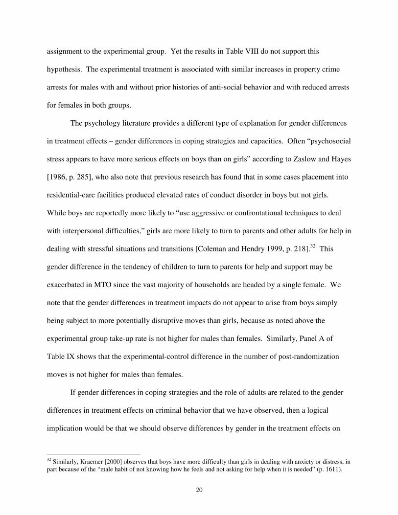
assignment to the experimental group. Yet the results in Table VIII do not support this

hypothesis. The experimental treatment is associated with similar increases in property crime

arrests for males with and without prior histories of anti-social behavior and with reduced arrests

for females in both groups.

The psychology literature provides a different type of explanation for gender differences

in treatment effects – gender differences in coping strategies and capacities. Often “psychosocial

stress appears to have more serious effects on boys than on girls” according to Zaslow and Hayes

[1986, p. 285], who also note that previous research has found that in some cases placement into

residential-care facilities produced elevated rates of conduct disorder in boys but not girls.

While boys are reportedly more likely to “use aggressive or confrontational techniques to deal

with interpersonal difficulties,” girls are more likely to turn to parents and other adults for help in

dealing with stressful situations and transitions [Coleman and Hendry 1999, p. 218].32 This

gender difference in the tendency of children to turn to parents for help and support may be

exacerbated in MTO since the vast majority of households are headed by a single female. We

note that the gender differences in treatment impacts do not appear to arise from boys simply

being subject to more potentially disruptive moves than girls, because as noted above the

experimental group take-up rate is not higher for males than females. Similarly, Panel A of

Table IX shows that the experimental-control difference in the number of post-randomization

moves is not higher for males than females.

If gender differences in coping strategies and the role of adults are related to the gender

differences in treatment effects on criminal behavior that we have observed, then a logical

implication would be that we should observe differences by gender in the treatment effects on

32 Similarly, Kraemer [2000] observes that boys have more difficulty than girls in dealing with anxiety or distress, in part because of the “male habit of not knowing how he feels and not asking for help when it is needed” (p. 1611).

21

measures of adult interaction among MTO youth.33 To examine this issue, we use the survey

data available for youth ages 15-20. Panel B of Table IX provides evidence for positive

treatment-control differences in youth interactions with adults for females but not males, which

is consistent with the coping hypothesis. In related work, Kling and Liebman [2004] find that

the MTO treatments improve mental health for female but not male youth.

On the other hand, we might expect gender differences in the ability to cope with stress

and change to lead to gender differences in arrests that are most pronounced during the period

shortly after families move through MTO. In this sense the psychological coping hypothesis

does not seem consistent with results in Table V, which show that in the short term, experimental

males experience fewer arrests than those in the control group, while the positive experimental-

control difference for males in property-crime arrests shows up only several years after random

assignment. The gender differences in neighborhood effects on adult interactions and mental

health may be a consequence rather than cause of gender differences in effects on youth crime.

Perhaps the best candidate explanation for our pattern of results is that experimental

youth have a comparative advantage in exploiting the set of theft opportunities available in their

new neighborhoods. Four years after random assignment, the average neighborhood property-

crime rate for experimental-group youth whose families moved through MTO is more than one-

quarter lower than for control-group youth (Table II). Some experimental-group youth who were

among the least criminally savvy in their old areas may be much more knowledgeable compared

33 We recognize that evidence for across-group differences in our mediating factors is not proof that one behavioral model or another is responsible for differences in youth anti-social behavior. Our reasoning is simply that if a treatment effect on an outcome is being driven by a particular mediating factor, then observing a treatment effect on that mediator would be a logically consistent pattern of results. When a mediating factor does not change as a result of MTO, we take this as evidence against that factor’s importance in explaining our particular results. Nevertheless, the factor may be an important mechanism outside of our experiment. Or within the experiment, if the average of a mediator was not changed by the treatment then it could still be the case that this factor is important because it interacts with treatment effect heterogeneity (e.g., among the treated, half experienced an increase in the mediator that contributed to a treatment effect on an outcome, while the other half experienced a decrease in the mediator unrelated to changes in outcomes). Conversely, when a mediating factor does change as a result of MTO, it is possible that it has no behavioral importance but is simply correlated with other important changes.

22

to the young people in their new neighborhoods. Experimental-group youth also moved into

schools containing peers with higher test scores on average [Sanbonmatsu et al. 2004]. Because

the experimental treatment did not appear to improve children’s own test scores, experimental-

group youth are on average at a lower point in their school’s achievement distribution compared

to youth in the control group. Thus, experimental movers may be relatively more competitive in

securing criminal rather than academic rewards in their new communities.

Why might boys be more likely than girls to exploit such a comparative advantage? The

answer does not seem to be gender differences in “criminal capital,” given the evidence

presented in Table VIII that gender differences in pre-program problem behavior do not explain

away gender differences in treatment effects on crime. But at least four other explanations are

plausible. First, experimental group boys have lower achievement test scores than do females,

with differences in reading and math scores of around .25 and .15 standard deviations,

respectively [Sanbonmatsu et al., 2004]. As a result, within the experimental group males on

average will be less academically competitive within their new schools than are females.

Second, adolescent boys tend to be subject to less parental supervision than girls [Block 1983;

Bottcher 2001], which is also true for our MTO youth sample: Table IX indicates that the

control mean for our survey measure of parental knowledge of who youth are with when not at

home is more than 40 percent higher for female youth compared to males. Third, the

psychological literature suggests that male youth may be more risk-taking than female youth, and

thus more criminally entrepreneurial [Block 1983; LaGrange and Silverman 1999]. Fourth,

overall gender differences in criminal offending within the general population may provide

experimental group boys with an easier time accessing a particularly important input into youth

crime – confederates [Reiss 1988; Zimring 1998].

23

Under the comparative advantage hypothesis we would expect the experimental treatment

to reduce pro-social behavior and peer affiliations for male youth. Panels C and D of Table IX

show that, consistent with this expectation, experimental boys experience an increase in school

absences relative to controls and an increase in their associations with anti-social peer groups, as

evidenced by the proportion of their friends who they report to use drugs. In contrast, the

experimental treatment produces an improvement in girls’ expectations for completing college

and participation in sports, a reduction in school absences and an increase in associations with

peers who engage in school activities. Although these predictions could also be generated by

alternative models of youth behavior, a strong argument for the comparative advantage

hypothesis is that it provides an explanation for the timing of the property-crime impact for

experimental group boys – specifically, the possibility that boys may require either some time to

learn their comparative advantage in their new neighborhoods or to recruit confederates.

V. CONCLUSION

Common wisdom within much of social science holds that residence within a high-crime,

disorganized, and disadvantaged urban community increases the propensity of youth to engage in

crime. Yet this belief rests almost entirely on empirical evidence that may confound the causal

effects of neighborhood context with those of unmeasured characteristics that are related to how

families sort themselves across neighborhoods.

Using exogenous variation in neighborhood characteristics generated by the MTO

randomized mobility experiment, we find gender differences in the relationship between

neighborhood context and youth crime for youth ages 15-25 year at the end of 2001 (who entered

MTO between ages 8 and 21). The offer to move to neighborhoods with lower rates of poverty

24

and crime produces reductions in criminal behavior for female youth, but produces mixed effects

on the behavior of male youth.34

Large reductions in the number of lifetime violent crime and property crime arrests were

found for females in the experimental group relative to the control group. Assignment to the

experimental group also appears to have produced reductions in violent-crime arrests among

males, at least in the short term, although these effects are proportionally smaller than those for

females. Moreover, four to seven years after random assignment, males in the experimental

group have scores on our behavior problem index that are about 20 percent higher than the

control group, and are also arrested for property offenses 30 percent more often than controls.

Assignment to the Section 8 group in general produces more modest differences in arrest rates

with the control group compared to the experimental-control differences, consistent with the fact

that the Section 8 treatment also produces more modest changes in neighborhood characteristics.

The main threats to internal validity with our estimates come from the possibility of self-

reporting bias with our survey data and from possible variation across areas in the probability of

arrest that may confound interpretation of results from official arrest data. Comparing the

lifetime prevalence of arrest in the survey and administrative data does provide some support for

the view that youth underreport anti-social behavior. However, for misreporting to explain our

findings, the treatment-control differences in misreporting tendencies would need to be exactly

opposite for females and males. In addition, the positive experimental-control difference in

property-crime arrests for male youth is mirrored by a similar increase in self-reported problem

behaviors suggesting the property-crime arrest results represent a real behavioral impact.

34 We note that it is still too early to learn about the long-run effects on criminal behavior of the MTO treatments on the younger MTO children (those under age 8 at random assignment). Also, MTO is a voluntary program, with eligibility limited to low-income public housing residents living in very disadvantaged communities. Other low-income populations may experience different behavioral changes in response to residential mobility.

25

What do these results tell us about the nature of neighborhood effects on youth crime?

For both male and female youths, moves through the MTO program change neighborhoods in

ways that “epidemic” models of neighborhood effects predict should reduce youth crime. While

these predictions are generally consistent with what is observed in the MTO data through the

first two years following random assignment, standard models of neighborhood effects

emphasizing the contagion effects of social interactions or the beneficial effects of neighborhood

institutions and adult role models in more affluent areas do not explain why problem behavior

and property crime should increase for experimental-group males relative to controls over the

medium-term. For these outcomes, the mechanisms appear to be more complex than postulated

in such models.

Female and male youth in MTO move into similar types of neighborhoods, so the gender

difference in MTO effects seems to reflect differential responses by male and female youths to

similar neighborhoods. This interpretation is consistent with more adverse treatment effects for

males in within-sibling comparisons. Discrimination is one possible mechanism that could

potentially lead to differential responses by gender, but we find little evidence of increased racial

discrimination for the experimental group relative to controls for either gender, presumably in

part because MTO produces surprisingly little racial integration.

Gender differences in adaptation to change in general and to new more-affluent

neighborhoods in particular are a more promising explanation for the gender differences in MTO

treatment effects on property crime. Previous findings in psychology suggest that males may

have more difficulty than females in adapting to change and stress, in part because female youth

are more likely to take advantage of adult support. These predictions are consistent with

observed gender differences in MTO treatment effects on youth interactions with adults (shown

in Table IX) and on mental health outcomes (reported by Kling and Liebman [2004]). However

26

this hypothesis does not seem to be fully consistent with our finding that violent-crime arrests

decline in the short term for experimental males relative to controls, and that property-crime

arrests increase for this group only a few years after randomization.

Arguably the best explanation for the pattern of neighborhood effects reported here is that

experimental-group youth may have a comparative advantage in exploiting the available

property-crime opportunities in their new neighborhoods, as economic theory might suggest.

Our data provide support for at least one explanation for why males may be more likely than

females to exploit this comparative advantage – differences in parental supervision. Other

candidate explanations for the gender difference in exploiting such a comparative advantage

include differences in academic achievement, risk taking, or, given the gender difference in

criminal offending in the population as a whole, the availability of confederates. In any case this

hypothesis, unlike the others mentioned above, provides a potential explanation for the timing of

the increase in property offending for experimental-group males, since it may take them some

time to learn and exploit their new comparative advantage.

What do our results imply for public policy? Should MTO be considered a “success” or a

“failure” with respect to the program’s ability to reduce crime by youth in participating families?

Focusing on the net change in the overall arrest rate across groups leads to a somewhat negative

answer to this last question, because the findings for violent-crime arrests among girls and boys

are generally offset by the effect on property-crime arrests among males. Yet, distributional

considerations aside, society is not indifferent towards the replacement of very damaging violent

crimes with less costly property offenses. Because violent crime imposes substantially higher

costs on society than do property offenses, on net increases in property crimes appear to be more

than offset by reductions in violent crime in our estimates of the aggregate social costs of crime

committed by MTO youth.

27

PRINCETON UNIVERSITY AND NATIONAL BUREAU OF ECONOMIC RESEARCH GEORGETOWN UNIVERSITY AND NATIONAL CONSORTIUM ON VIOLENCE RESEARCH HARVARD UNIVERSITY AND NATIONAL BUREAU OF ECONOMIC RESEARCH

REFERENCES Akerlof, George A. and Rachel E. Kranton, “Economics and Identity,” Quarterly Journal of

Economics, CXV (2000), 715-754. Angrist, Joshua A., Guido W. Imbens, and Donald B. Rubin, “Identification of Causal Effects

Using Instrumental Variables,” Journal of the American Statistical Association, XCI (1996), 444-472.

Bertrand, Marianne and Sendhil Mullainathan, “Are Emily and Greg More Employable than Lakisha and Jamal? A Field Experiment on Labor Market Discrimination,” American Economic Review, XCIII (2004), forthcoming.

Block, Jeanne H., “Differential Premises Arising from Differential Socialization of the Sexes: Some Conjectures,” Child Development, LIV (1983), 1335-1354.

Bloom, Howard, “Accounting for No-Shows in Experimental Evaluation Designs,” Evaluation Review, VIII (1984), 225-46.

Blumstein, Alfred and Joel Wallman, eds., The Crime Drop in America (New York: Cambridge University Press, 2000).

Bottcher, Jean, “Social Practices of Gender: How Gender Relates to Delinquency in the Everyday Lives of High-Risk Youths,” Criminology, XXXIX (2001), 893-931.

Coleman, James S., The Adolescent Society, (NY: Free Press, 1961). Coleman, John and Leo B. Hendry, The Nature of Adolescence, Third Edition (London:

Routledge, 1999). Cook, Philip J., “The Demand and Supply of Criminal Opportunities,” in M. Tonry and N.

Morris, eds., Crime and Justice: An Annual Review of Research (Chicago: University of Chicago Press, 1986), 1-27.

Cook, Philip J., “The Technology of Personal Violence,” in M. Tonry, ed., Crime and Justice: An Annual Review of Research (Chicago: University of Chicago Press, 1991), 1-71.

Cook, Philip J. and Kristin A. Goss, “A Selective Review of the Social-Contagion Literature,” Working Paper, Sanford Institute of Public Policy Studies, Duke University, 1996.

Cook, Philip J. and John Laub, “The Unprecedented Epidemic in Youth Violence,” in M. Tonry, ed., Crime and Justice: An Annual Review of Research (Chicago: University of Chicago Press, 1998), 26-64.

Cutler, David M., Edward L. Glaeser and Jacob L. Vigdor, “The Rise and Decline of the American Ghetto,” Journal of Political Economy, CVII (1999), 455-506.

Darity, William A. and Patrick L. Mason, “Evidence on Discrimination in Employment: Codes of Color, Codes of Gender,” Journal of Economic Perspectives, XII (1998), 63-90.

Dunworth, Terence and Aaron Saiger, Drugs and Crime in Public Housing: A Three-City Analysis (Washington, DC: National Institute of Justice, 1994).

Ehrlich, Issac, “On the Usefulness of Controlling Individuals: An Economic Analysis of Rehabilitation, Incapacitation and Deterrence,” American Economic Review, LXXII (1981), 307-322.

28

Ehrlich, Isaac, “Crime, Punishment and the Market for Offenses,” Journal of Economic Perspectives, X (1996), 43-68.

Fox, James A., and Marianne W. Zawitz. Homicide Trends in the United States (Washington, DC: Bureau of Justice Statistics, 2002).

Glaeser, Edward L., Bruce Sacerdote, and Jose A. Scheinkman, “Crime and Social Interactions.” Quarterly Journal of Economics, CXI (1996), 507-548.

Glaeser, Edward L. and Jacob L. Vigdor, Racial Segregation in the 2000 Census: Promising News (Washington, DC: Brookings Institution, 2001).

Haines, Michael R., “Ethnic Differences in Demographic Behavior in the United States: Has There Been Convergence?,” Cambridge, MA: NBER WP No. 9042, July 2002.

Jencks, Christopher and Susan E. Mayer, “The Social Consequences of Growing Up in a Poor Neighborhood,” in L. Lynn and M. McGeary, eds., Inner-City Poverty in the United States (Washington, DC: National Academy of Sciences, 1990).

Johnson, William R. and Derek Neal, “Basic Skills and the Black-White Earnings Gap,” in C. Jencks and M. Phillips, eds., The Black White Test Score Gap (Washington, DC: Brookings Institution, 1998), 480-500.

Katz, Lawrence F., Jeffrey R. Kling, and Jeffrey B. Liebman, “Moving to Opportunity in Boston: Early Results of a Randomized Mobility Experiment,” Quarterly Journal of Economics, CXVI (2001), 607-654.

Kirschenman, Joleen and Kathryn M. Neckerman, “ ‘We’d Love to Hire Them, But…’: The Meaning of Race for Employers,” in C. Jencks and P. Peterson, eds., The Urban Underclass (Washington, DC: Brookings Institution Press, 1991).

Kling, Jeffrey R., and Jeffrey B. Liebman, “Experimental Analysis of Neighborhood Effects on Youth,” Princeton IRS Working Paper 483, April 2004.

Kling, Jeffrey R., Jens Ludwig, and Lawrence F. Katz, “Youth Criminal Behavior in the Moving to Opportunity Experiment,” Princeton IRS Working Paper 482, March 2004.

Kraemer, Sebastian, “The Fragile Male,” British Medical Journal, 321 (2000), 23-30. LaGrange, Teresa C. and Robert A. Silverman, “Low Self-Control and Opportunity: Testing the

General Theory of Crime as an Explanation for the Gender Differences in Delinquency,” Criminology, XXXVII (1999), 41-72.

Leventhal, Tama and Jeanne Brooks-Gunn, “New York City Site Findings: The Early Impacts of Moving to Opportunity on Children and Youth,” in J. Goering and J. Feins, eds., Choosing a Better Life: Evaluating the Moving to Opportunity Social Experiment (Washington, DC: Urban Institute Press, 2003), 213-244.

Levitt, Steven D., “Understanding Why Crime Fell in the 1990’s: Four Factors that Explain the Decline and Six that Do Not,” Journal of Economic Perspectives, XVIII (2004), 163-190.

Ludwig, Jens, Greg J. Duncan, and Paul Hirschfield, “Urban Poverty and Juvenile Crime: Evidence from a Randomized Housing-Mobility Experiment,” Quarterly Journal of Economics, CXVI (2001), 655-680.

Ludwig, Jens, Brian A. Jacob, Greg J. Duncan, James Rosenbaum, Michael Johnson, “The Effects of Housing Vouchers on Criminal Behavior: Evidence from a Randomized Lottery,” Working Paper, Georgetown University Public Policy Institute, 2004.

Maguire, Kathleen, and Anne L. Pastore, Bureau of Justice Statistics Sourcebook of Criminal Justice Statistics—1998 (Washington, DC: Government Printing Office, 1999).

Maltz, Michael D., “Bridging Gaps in Police Crime Data, NCJ 176365,” (Washington, DC: Bureau of Justice Statistics, 1999).

29

Massey, Douglas S. and Mary J. Fischer, “The Geography of Inequality in the United States, 1950-2000,” in W. Gale and J. Pack, eds., Brookings-Wharton Papers on Urban Affairs (Washington, DC: Brookings Institution, 2003).

Miller, Ted R., Mark A. Cohen, and Brian Wiersema, Victim Costs and Consequences: A New Look (Washington, DC: National Institute of Justice, NCJ 155282, 1996).

Neal, Derek A. and William R. Johnson, “The Role of Premarket Factors in Black-White Wage Differences,” Journal of Political Economy, CIV (1996), 869-895.

Olsen, Edgar O., “Housing Programs for Low-Income Households,” in R. Moffitt, ed., Means-Tested Transfer Programs in the Untied States (Chicago: University of Chicago Press and NBER, 2003).

Orr, Larry et al., Moving to Opportunity: Interim Impacts Evaluation (Washington, DC: U.S. Department of Housing and Urban Development, Office of Policy Development and Research, 2003).

Reiss, Albert J., “Co-Offending and Criminal Careers,” in Michael Tonry and Norval Morris, eds., Crime and Justice: An Annual Review of Research (Chicago, IL: University of Chicago Press, 1988).

Sah, Raaj K., “Social Osmosis and Patterns of Crime,” Journal of Political Economy, XCIX (1991), 1272-1295.

Sampson, Robert J., Jeffrey D. Morenoff, and Thomas Gannon-Rowley, “Assessing ‘Neighborhood Effects’: Social Processes and New Directions in Research,” Annual Review of Sociology, XXVIII (2002), 443-478.

Sampson, Robert J., Stephen W. Raudenbush, and Felton Earls, “Neighborhoods and Violent Crime: A Multilevel Study of Collective Efficacy,” Science, CCLXXVII (1997), 918-924.

Sanbonmatsu, Lisa, Jeanne Brooks-Gunn, Greg J. Duncan, and Jeffrey R. Kling, “Neighborhoods and Academic Achievement: Results from the MTO Experiment,” Princeton IRS Working Paper 492, July 2004.

Tracy, Paul E., Marvin E. Wolfgang, and Robert M. Figlio, Delinquency Careers in Two Birth Cohorts (New York: Plenum Press, 1990).

Watson, Tara, “Inequality and the Rising Segregation of American Neighborhoods,” unpublished paper, Harvard University, 2003.

Wilson, William J. The Truly Disadvantaged (Chicago: University of Chicago Press, 1987). Wolfgang, Marvin E., Robert M. Figlio, Paul E. Tracy and Simon J. Singer. The National

Survey of Crime Severity, NCJ-96017 (Washington, DC: U.S. Department of Justice, 1985).

Zaslow, Martha J. and Cheryl D. Hayes, “Sex Differences in Children’s Response to Psychosocial Stress: Toward a Cross-Context Analysis,” in M. Lamb, A. Brown and B. Rogoff, eds., Advances in Developmental Psychology, Volume 4 (Hillsdale, NJ: Lawrence Earlbaum, 1986), 285-338.

Zimring, Franklin E., American Youth Violence (New York: Oxford University Press, 1998).

30

Figure 1: Homicide Offending Rates for Black Males and Females 18-24 from 1976 to 2000

0

50

100

150

200

250

300

350

400

1976

1979

1982

1985

1988

1991

1994

1997

2000

Hom

icid

e O

ffend

ing

Rat

e pe

r 10

0,00

0

Black male 18-24

Black female 18-24

Notes. Data taken from FBI’s Supplemental Homicide Reports, 1976-2000 [Fox and Zawitz 2002].

31

TABLE I BASELINE CHARACTERISTICS OF SURVEY AND ADMINISTRATIVE DATA SAMPLES

Admin Data Sample (Ages 15-25) Survey Sample (Ages 15-20)

Baseline Characteristic Control Experimental Section 8 Control Experimental Section 8

A. Household characteristics

Head education:

GED .19 .16 .17 .17 .16 .17

High school .30 .34 .32 .37 .39 .40

Head was teen parent .28 .27 .27 .25 .26 .25

Household on AFDC .74 .74 .73 .75 .76 .74 Primary/secondary

reason for enrolling:

Gangs, drugs .78 .80 .74 .78 .79 .74

Better schools .50 .48 .53 .51 .50 .58

B. Youth characteristics

Male .51 .50 .51 .49 .49 .48

Age in years on 12/31/01 19.4 19.5 19.3 17.6 17.7 17.7

African-American .62 .62 .61 .63 .66 .65

Hispanic .33 .31 .32 .31 .32 .32

Behavior problems .08 .09 .09 .07 .12 .12

Expelled from school .14 .16 .14 .11 .16 .15

In gifted program .17 .15 .17 .22 .16 .16

Learning problems .19 .20 .17 .21 .21 .19

Ever arrested .09 .11 .08 .03 .04 .04

N 1367 1840 1266 548 749 510

Notes. Administrative data sample consists of all MTO youth ages 15-25 on 12/31/01, with means in this table calculated just for those MTO youth who are ages 15-25 at the end of 2001 and under age 18 at baseline, and so for whom baseline survey results on these measures are available. Survey sample consists of respondents ages 15-20 on 12/31/01, in which the survey randomly selected up to two children per household. Data are from MTO baseline survey, except for “ever arrested,” which is from administrative records. Behavior/Learning problems = gone to a special class or school or gotten special help in school for behavior/learning problems in two years prior to baseline. “Hispanic” includes both black and non-black Hispanics.

32

TABLE II NEIGHBORHOOD CHARACTERISTICS FOR MTO YOUTH AFTER RANDOM ASSIGNMENT

Control Experimental Section 8

All All Move All Move 1 2 3 4 5

A. Census Tracts 1 Year After RA

Average Tract Poverty Rate .47 .34 .16 .36 .29

Tract poverty rate .40+ .67 .41 .08 .40 .19

Tract poverty rate .20 - .40 .26 .23 .11 .42 .51

Tract poverty rate 0 - .20 .07 .36 .81 .19 .30

B. Census Tracts 4 Years After RA

Average Tract Poverty Rate .42 .32 .18 .34 .28

Tract poverty rate .40+ .53 .33 .06 .33 .18

Tract poverty rate .20 - .40 .34 .34 .27 .43 .51

Tract poverty rate 0 - .20 .13 .34 .66 .23 .31

Fraction on welfare .19 .14 .07 .15 .13

Fraction of female headed households .58 .50 .35 .52 .47

Fraction of youth not in labor force .12 .11 .09 .11 .11

Fraction minority .90 .84 .74 .87 .86

Local area violent crime rate per 10K 234 203 128 204 211

Local area property crime rate per 10K 512 488 371 481 529

C. Adult report on neighborhood in 2002

Neighbors would not likely do something about truant children

.65 .53 .43 .57 .58

Neighbors would not likely do something about spraying of graffiti

.47 .36 .26 .41 .40

Problem in neighborhood with graffiti .48 .38 .19 .40 .32

Problem in neighborhood with police not coming when called

.33 .22 .11 .27 .23

Number of youth ages 15-25 1367 1840 772 1266 663

Notes. Move = youth in households moving through MTO. Census tract characteristics calculated using 2000 Census data. Sample for panels A and B is based on locations for individuals ages 15-25 on 12/31/01 obtained from the survey and from other tracking methods, and excludes individuals for whom we are missing juvenile crime records. Sample for panel C is adults with at least one youth ages 15-25 on 12/31/01 who does not have missing juvenile crime records.

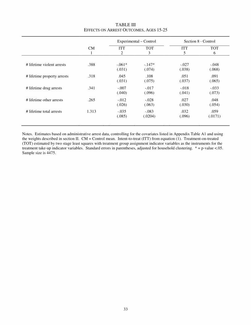
33

TABLE III EFFECTS ON ARREST OUTCOMES, AGES 15-25

Notes. Estimates based on administrative arrest data, controlling for the covariates listed in Appendix Table A1 and using the weights described in section II. CM = Control mean. Intent-to-treat (ITT) from equation (1). Treatment-on-treated (TOT) estimated by two stage least squares with treatment group assignment indicator variables as the instruments for the treatment take-up indicator variables. Standard errors in parentheses, adjusted for household clustering. * = p-value <.05. Sample size is 4475.

Experimental – Control Section 8 - Control

CM ITT TOT ITT TOT 1 2 3 5 6

# lifetime violent arrests

.388 -.061* (.031)

-.147* (.074)

-.027 (.038)

-.048 (.068)

# lifetime property arrests

.318 .045 (.031)

.108 (.075)

.051 (.037)

.091 (.065)

# lifetime drug arrests

.341 -.007 (.040)

-.017 (.096)

-.018 (.041)

-.033 (.073)

# lifetime other arrests

.265 -.012 (.026)

-.028 (.063)

.027 (.030)

.048 (.054)

# lifetime total arrests

1.313 -.035 (.085)

-.083 (.0204)

.032 (.096)

.059 (.0171)

34

TABLE IV EFFECTS ON ARRESTS, DELINQUENCY, AND PROBLEM BEHAVIOR BY GENDER

Females Males Male-Female

CM ITT TOT CM ITT TOT ITT TOT 1 2 3 4 5 6 8 9

A. Exp-Control, Ages 15-25

# lifetime violent arrests n=4,475

.241 -.077* (.031)

-.185* (.076)

.537 -.045 (.051)

-.107 (.123)

.031 (.057)

.078 (.140)

# lifetime property arrests n=4,475

.164 -.057* (.026)

-.140* (.065)

.474 .150* (.055)

.363* (.136)

.207* (.060)

.503* (.148)

# lifetime drug arrests n=4,475

.087 -.060 (.034)

-.143 (.082)

.597 .047 (.071)

.112 (.171)

.106 (.076)

.256 (.186)

# lifetime other arrests n=4,475

.119 -.032 (.020)

-.077 (.049)

.413 .009 (.046)

.023 (.111)

.040 (.047)

.099 (.115)

# lifetime total arrests n=4,475

.611 -.225* (.071)

-.545* (.176)

2.021 .160 (.150)

.391 (.364)

.385* (.160)

.936* (.394)

B. Exp-Control, Ages 15-20

# lifetime total arrests n=3,079

.531 -.186* (.078)

-.430* (.186)

1.382 .279 (.150)

.637 (.339)

.465* (.164)

1.067* (.379)

Ever arrested n=3,079

.245 -.029 (.025)

-.067 (.059)

.390 .053 (.028)

.120 (.063)

.082* (.036)

.187* (.085)

Ever arrested [SR] n=1,790

.126 -.015 (.028)

-.032 (.060)

.289 .013 (.041)

.032 (.100)

.028 (.049)

.065 (.115)

Delinquency index [SR] n=1,795

.070 -.008 (.011)

-.016 (.023)

.136 .002 (.018)

.005 (.044)

.009 (.020)

.021 (.048)

Behavior prob index [SR] n=1,795

.340 -.019 (.023)

-.039 (.050)

.343 .064* (.025)

.160* (.062)

.082* (.033)

.199* (.080)

C. Sec8 - Control, Ages 15-25

# lifetime violent arrests n=4,475

.241 -.079* (.036)

-.143* (.065)

.537 .024 (.062)

.046 (.113)

.103 (.069)

.188 (.125)

# lifetime property arrests n=4,475

.164 .031 (.039)

.053 (.070)

.474 .072 (.059)

.127 (.106)

.041 (.068)

.074 (.124)

# lifetime drug arrests n=4,475

.087 .019 (.040)

.035 (.072)

.597 -.055 (.075)

-.100 (.135)

-.075 (.089)

-.135 (.161)

# lifetime other arrests n=4,475

.119 .018 (.024)

.031 (.042)

.413 .036 (.054)

.065 (.098)

.018 (.059)

.034 (.107)

# lifetime total arrests n=4,475

.611 -.012 (.089)

-.024 (.160)

2.021 .076 (.170)

.138 (.306)

.087 (.193)

.162 (.351)

D. Sec8 - Control, Ages 15-20

# lifetime total arrests n=3,079

.531 -.139 (.093)

-.239 (.162)

1.382 .258 (.174)

.455 (.305)

.396* (.197)

.694* (.347)

Ever arrested n=3,079

.245 -.059* (.027)

-.100* (.047)

.390 .047 (.032)

.083 (.056)

.106* (.040)

.184* (.071)

Ever arrested [SR] n=1,790

.126 -.012 (.032)

-.020 (.054)

.289 .026 (.049)

.050 (.091)

.038 (.058)

.069 (.106)

Delinquency index [SR] n=1,795

.070 -.005 (.012)

-.008 (.021)

.136 .013 (.022)

.025 (.041)

.018 (.023)

.033 (.043)

Behavior prob index [SR] n=1,795

.340 -.009 (.024)

-.015 (.042)

.343 .031 (.028)

.060 (.053)

.039 (.035)

.074 (.066)

Notes. Unless otherwise indicated, estimates based on administrative arrest data, using the covariates from Appendix Table A1 and weights described in section II. SR = self-report. Intent-to-treat (ITT) from equation (2). Treatment-on-treated (TOT) estimated by two stage least squares with treatment group assignment indicator variables as the instruments for the treatment take-up indicator variables. Standard errors in parentheses, adjusted for household clustering. * = p-value <.05.

35

TABLE V

EFFECTS ON ANNUAL ARRESTS BY YEAR SINCE RANDOM ASSIGNMENT, AGES 15-25 Females Males Male-Female

CM E-C S-C CM E-C S-C E-C S-C 1 2 3 4 5 6 8 9

A. Violent arrests

1-2 years since RA .0282 -.0091 (.0073)

-.0109 (.0084)

.0725 -.0248* (.0124)

-.0099 (.0132)

-.0156 (.0136)

.0011 (.0149)

3-4 years since RA .0375 -.0071 (.0082)

-.0048 (.0094)

.0730 -.0099 (.0123)

.0110 (.0146)

-.0028 (.0140)

.0157 (.0163)

1-4 years since RA .0332 -.0080 (.0061)

-.0077 (.0073)

.0728 -.0168 (.0095)

.0012 (.0111)

-.0088 (.0107)

.0089 (.0125)

B. Property arrests

1-2 years since RA .0225 -.0120 (.0063)

.0019 (.0088)

.0614 -.0107 (.0121)

-.0062 (.0127)

.0013 (.0126)

-.0081 (.0141)

3-4 years since RA .0299 -.0135 (.0075)

.0016 (.0095)

.0707 .0374* (.0135)

.0134 (.0144)

.0509* (.0149)

.0118 (.0165)

1-4 years since RA .0265 -.0132* (.0053)

.0015 (.0077)

.0664 .0149 (.0100)

.0042 (.0100)

.0281* (.0107)

.0027 (.0118)

C. Total arrests

1-2 years since RA .0707

-.0311* (.0127)

-.0068 (.0154)

.2296 -.0262 (.0262)

.0003 (.0279)

.0050 (.0278)

.0071 (.0302)

3-4 years since RA .1025 -.0295 (.0165)

.0147 (.0202)

.3018 .0479 (.0346)

.0188 (.0357)

.0775* (.0375)

.0041 (.0402)

1-4 years since RA .0877 -.0308* (.0121)

.0044 (.0152)

.2681 .0133 (.0255)

.0101 (.0262)

.0441 (.0273)

.0057 (.0293)

Notes. E-C = Experimental ITT effect. S-C = Section 8 ITT effect. RA = Date of random assignment. Estimates are calculated using a panel of person-quarter observations, and results are re-scaled to represent the number of arrests per person per year, as described in the text. Arrest data are from administrative records. Covariates are those in Appendix Table A1 and indicator variables for calendar quarter and time since random assignment. Weights are as described in section II. Standard errors in parentheses are adjusted for correlation in outcomes across time periods among youth from the same household. * = p-value <.05. Sample size is 2252 females and 2221 males.

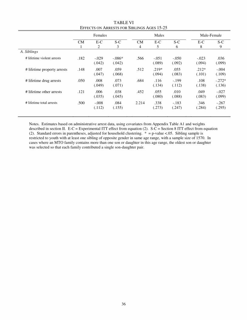
36

TABLE VI

EFFECTS ON ARRESTS FOR SIBLINGS AGES 15-25 Females Males Male-Female

CM E-C S-C CM E-C S-C E-C S-C 1 2 3 4 5 6 8 9

A. Siblings

# lifetime violent arrests .182 -.029 (.042)

-.086* (.042)

.566 -.051 (.089)

-.050 (.092)

-.023 (.094)

.036 (.099)

# lifetime property arrests .148 .007 (.047)

.059 (.068)

.512 .219* (.094)

.055 (.083)

.212* (.101)

-.004 (.109)

# lifetime drug arrests .050 .008 (.049)

.073 (.071)

.684 .116 (.134)

-.199 (.112)

.108 (.138)

-.272* (.136)

# lifetime other arrests .121 .006 (.035)

.038 (.045)

.452 .055 (.080)

.010 (.088)

.049 (.083)

-.027 (.099)

# lifetime total arrests .500 -.008 (.112)

.084 (.155)

2.214 .338 (.273)

-.183 (.247)

.346 (.284)

-.267 (.295)

Notes. Estimates based on administrative arrest data, using covariates from Appendix Table A1 and weights described in section II. E-C = Experimental ITT effect from equation (2). S-C = Section 8 ITT effect from equation (2). Standard errors in parentheses, adjusted for household clustering. * = p-value <.05. Sibling sample is restricted to youth with at least one sibling of opposite gender in same age range, with a sample size of 1570. In cases where an MTO family contains more than one son or daughter in this age range, the oldest son or daughter was selected so that each family contributed a single son-daughter pair.

37

TABLE VII EFFECTS RELATED TO DISCRIMINATION, AGES 15-20

Females Males Male-Female

CM E-C S-C CM E-C S-C E-C S-C 1 2 3 4 5 6 8 9

A. Census tract composition 4 years after RA

Fraction black n=1801

.524 -.019 (.023)

.006 (.024)

.514 -.034 (.022)

-.088* (.031)

-.015 (.030)

-.095* (.037)

Fraction minority n=1801

.904 -.064* (.018)

-.022 (.019)

.898 -.066* (.020)

-.069* (.028)

-.002 (.025)

-.047 (.033)

Fraction above 50% minority n=1801

.946 -.076* (.024)

-.026 (.025)

.918 -.057 (.030)

-.059 (.037)

.019 (.036)

-.034 (.043)

Fraction above 75% minority n=1801

.902 -.139* (.032)

-.058 (.032)

.883 -.115* (.035)

-.100* (.042)

.024 (.044)

-.041 (.051)

B. Racial discrimination

Treated unfairly because of race at work or school n=1793

.132 -.030 (.028)

-.001 (.032)

.146 -.023 (.034)

.001 (.042)

.007 (.044)

.002 (.051)

Treated unfairly because of race while shopping n=1797

.153 -.020 (.030)

.029 (.035)

.114 .020 (.029)

.052 (.038)

.040 (.041)

.023 (.053)

Treated unfairly because of race by police n=1791

.074 -.002 (.022)

-.018 (.023)

.193 -.060 (.034)

-.002 (.044)

-.058 (.040)

.016 (.049)

C. Census tract affluence 4 years after RA

Fraction professional or managerial job n=1800

.200 .051* (.010)

.029* (.011)

.216 .035* (.011)

.005 (.011)

-.016 (.015)

-.024 (.015)

Fraction college degree n=1801

.128 .061* (.012)

.033* (.012)

.139 .049* (.012)

.021 (.012)

-.012 (.016)

-.012 (.016)

D. Class discrimination

Trouble getting along with teachers n=1778

.235 .033 (.038)

-.008 (.042)

.300 .046 (.042)

.012 (.046)

.012 (.058)

.020 (.061)

Agrees that discipline in school is fair, ages 15-18 n=1199

.660 .047 (.055)

.007 (.058)

.675 .049 (.053)

-.019 (.064)

.003 (.077)

-.026 (.085)

5+ friends n=1793

.382 .060 (.044)

.048 (.047)

.530 .024 (.049)

.072 (.053)

-.037 (.066)

.024 (.070)

Lives in or visits friends in baseline neighborhood n=1744

.700 -.143* (.044)

-.140* (.046)

.699 -.060 (.045)

-.086 (.052)

.083 (.062)

.054 (.068)

Got in fight in past 12 months n=1795

.169 .019 (.033)

-.010 (.035)

.244 .065 (.041)

.022 (.044)

.046 (.052)

.032 (.055)

Felt worthless in past 30 days n=1792

.276 -.066 (.037)

-.041 (.042)

.168 .003 (.035)

-.028 (.037)

.069 (.051)

.013 (.056)

Satisified with neighborhood n=1724

.457 .099* (.048)

.043 (.052)

.570 -.022 (.049)

-.023 (.054)

-.121 (.068)

-.066 (.074)

Notes. Estimates based on survey data and Census data linked to geocoded location, using covariates in Appendix Table A1 and weights described in section II. CM = control mean. E-C = Experimental ITT effect from equation (2). S-C = Section 8 ITT effect from equation (2). Standard errors are in parentheses, adjusted for household clustering. * = p-value <.05.

38

TABLE VIII EFFECTS ON ARRESTS BY PROBLEM BEHAVIOR HISTORY, AGES 15-25

Females Males Male-Female

CM E-C S-C CM E-C S-C E-C S-C 1 2 3 4 5 6 8 9

A. Prior history of anti-social behavior

# lifetime violent arrests .428 -.070 (.090)

-.022 (.107)

.866 -.086 (.097)

.074 (.115)

-.016 (.135)

.096 (.157)

# lifetime property arrests .356 -.088 (.074)

.083 (.106)

.690 .154 (.102)

.087 (.111)

.242 (.127)

.005 (.158)

# lifetime drug arrests .088 .031 (.068)

.244* (.100)

.876 .028 (.128)

-.163 (.133)

-.003 (.146)

-.407* (.173)

# lifetime other arrests .220 -.027 (.053)

.049 (.061)

.637 -.098 (.080)

.052 (.108)

-.071 (.095)

.003 (.124)

# lifetime total arrests 1.108 -.112 (.180)

.368 (.340)

3.107 .056 (.272)

.091 (.303)

.167 (.328)

-.278 (.396)

B. No prior history of anti-social behavior

# lifetime violent arrests .193 -.071* (.035)

-.111* (.038)

.244 .004 (.055)

.016 (.073)

.076 (.064)

.126 (.081)

# lifetime property arrests .111 -.041 (.027)

0 (.038)

.241 .152* (.060)

.096 (.068)

.193* (.064)

.096 (.075)

# lifetime drug arrests .094 -.069 (.041)

-.054 (.039)

.341 .013 (.079)

-.006 (.090)

.082 (.086)

.048 (.098)

# lifetime other arrests .072 -.044* (.020)

-.003 (.021)

.188 .012 (.047)

-.017 (.051)

.056 (.050)

-.015 (.056)

# lifetime total arrests .480 -.216* (.080)

-.167 (.089)

1.014 .192 (.164)

.102 (.200)

.408* (.179)

.269 (.220)

Notes. Estimates based on administrative arrest data, using covariates from Appendix Table A1 and weights described in section II. E-C = Experimental ITT effect from equation (2). S-C = Section 8 ITT effect from equation (2). Standard errors in parentheses, adjusted for household clustering. * = p-value <.05 Prior history of anti-social behavior is defined as whether the teen had been arrested, expelled, provided with services for a behavior problem, or had his parents called to school for some type of problem. Sample is restricted to youth who are both 15-25 at the end of 2001 and were under 18 at the time of enrolling in MTO, for whom therefore pre-program problem behavior information is available from the baseline surveys. Among males, 1008 have prior history while 1172 do not; for females 585 have a prior history and 1619 do not.

39

TABLE IX

EFFECTS RELATED TO ADAPTATION, AGES 15-20 Females Males Male-Female

CM E-C S-C CM E-C S-C E-C S-C 1 2 3 4 5 6 8 9

A. General Mobility Outcomes

MTO take-up rate

0 .461* (.033)

.595* (.038)

0 .415* (.032)

.542* (.039)

-.046 (.043)

-.053 (.052)

# Moves since RA

1.014 .496* (.090)

.573* (.100)

1.198 .193 (.104)

.223* (.114)

-.302* (.130)

-.350* (.144)

B. Interaction with adults

Parent knows everything about who with when not home n=1793

.385 .036 (.045)

-.030 (.046)

.270 -.015 (.043)

-.016 (.049)

-.051 (.060)

.014 (.065)

Sees father at least once a week n=1778

.253 .075 (.040)

.094* (.044)

.365 -.024 (.044)

.010 (.049)

-.098 (.058)

-.083 (.065)

3+ adults to confide in n=1797

.305 .140* (.042)

.070 (.046)

.397 -.001 (.048)

.027 (.052)

-.141* (.063)

-.043 (.068)

Structured after school activity with adults n=1753

.275 .063 (.043)

-.002 (.042)

.248 .043 (.041)

.057 (.047)

-.020 (.059)

.059 (.062)

C. Pro-social engagement

Employed n=1797

.281 -.017 (.040)

-.048 (.043)

.210 -.016 (.037)

.017 (.041)

.001 (.055)

.065 (.059)

In school or employed n=1803

.771 .067 (.036)

-.002 (.038)

.758 .007 (.036)

.002 (.041)

-.060 (.051)

.005 (.055)

Believes chances are high of completing college n=1778

.543 .096* (.045)

.043 (.050)

.449 -.044 (.046)

-.049 (.049)

-.139* (.065)

-.092 (.070)

Works very hard on schoolwork n=1211

.508 .052 (.056)

.001 (.060)

.449 -.103 (.056)

.013 (.066)

-.155* (.078)

.012 (.088)

Fraction of days absent n=1649

.074 -.020* (.009)

-.015 (.009)

.057 .021* (.009)

.011 (.010)

.041* (.013)

.026* (.013)

Participates in sports after school n=1707

.032 .047* (.024)

.002 (.018)

.138 .003 (.032)

.031 (.038)

-.044 (.040)

.029 (.043)

D. Peers

Has friends who use drugs n=1698

.295 .007 (.043)

.029 (.046)

.327 .118* (.048)

.134* (.053)

.111 (.063)

.105 (.069)

Has friends who carry weapons n=1731

.098 .007 (.026)

.027 (.031)

.157 .037 (.040)

-.052 (.039)

.030 (.046)

-.080 (.050)

Has friends who participate in school activities n=1729

.615 .092* (.046)

.036 (.049)

.710 -.007 (.044)

-.011 (.049)

-.099 (.064)

-.047 (.070)

Notes. Estimates based on survey data and address history data from the MTO tracking file, using covariates from Appendix Table A1 and weights described in section II. CM = control mean. E-C = Experimental ITT effect from equation (2). S-C = Section 8 ITT effect from equation (2). Standard errors are in parentheses, adjusted for household clustering. * = p-value <.05.

40

APPENDIX A: DATA APPENDIX

This appendix provides information about our survey data, local area crime rate data, and

administrative data on arrests. Further details and site-specific information are available in

Appendix A of Kling, Ludwig, and Katz [2004].

1. Survey data

Baseline survey data was collected for each household randomly assigned during 1994-

97. Data from these baseline surveys is the basis for the covariates listed in Appendix Table A1.

Address histories for each sample member were also tracked through program operations, credit

bureaus, National Change of Address, housing authorities, and in-person tracking for this study.

In collaboration with HUD and Abt Associates, during 2002 our research team collected

survey data from one adult and two randomly selected children in each MTO household. The

surveys covered a wide range of topics including child behavior, housing, neighborhoods, health,

education, social interactions, employment and public assistance receipt [Orr et al. 2003].

In this paper we focus on surveys with about 1800 youth who were ages 15-20 at the end

of 2001. Data come from interviews with an adult in their household (usually the mother), and

from the youth themselves. The data were collected in two phases. In our main phase, we

attempted to collect data from 10931 children ages 5-20 and from adults from the 4248

households randomly assigned to MTO as of December 31, 1997. This data collection effort

extended from December 2001 - July 2002, and we completed data collection with 78 percent of

the sample. We refer to this as our Initial Response Rate (IRR). Among all individuals without

completed surveys at that time, we drew a 3-in-10 subsample to concentrate our remaining

resources on finding hard-to-locate families in a way that would minimize the potential for non-

response bias in our analyses. Between July 2002 and September 2002, we completed surveys

41

with 49 percent of the subsample. We refer to this as our Subsample Response Rate (SRR).

Since the subsample members are representative of all nonrespondents from the initial phase, we

combine them to report an overall Effective Response Rate; ERR = IRR+(1-IRR)*SRR. For the

study overall, the ERR is therefore about 89 percent.

The ERR for our youth sample specifically is around 88 percent, and is slightly higher

for females (90 percent) than males (86 percent). The youth response rates are quite similar

across MTO groups, equal to 87 percent for the experimental and control groups and 90 percent

for the Section 8 group. Interviewers were not informed about the random assignment group of

the respondent, though in some cases they may have been able to infer it. Because the number

of youth respondents at each site is relatively modest, in our analysis we focus on the pooled

sample of youth across all five sites.

2. Local-area crime rate data

To measure how MTO impacts participants’ exposure to crime, we obtained local-area

crime and population data for 1994 through 2001. We focus on those FBI Part I Index offenses

with consistent data across areas: the violent index offenses of murder, rape, robbery, and

aggravated assault, as well as the property offenses of burglary, motor vehicle theft, and larceny.

Each MTO address located within the five original demonstration cities was geo-coded and

assigned the crime rate of the police “beat” in which that address was located. The resolution

provided by this beat-level data varies across cities: Baltimore has 9 police beats, while Boston

has 11, Chicago 279, Los Angeles 18, and New York City 76. Addresses that could not be geo-

coded were assigned the city’s overall crime rate.

Addresses located outside of the five original MTO cities were assigned either place- or

county-level crime data, depending on whether the municipality in which the address is located

42

is patrolled by a local or a county law enforcement agency. These crime figures come from the

FBI’s Uniform Crime Reporting system, which is subject to a number of well-known problems

such as non-reporting or incomplete reporting. Our results for MTO’s impact on local-area

crime rates do not appear to be sensitive to how we handle these reporting problems.35

We end up with local-area criminal justice data for nearly 47000 of the 48751 MTO

address spells for 1997-2001, with figures that run a bit lower for 1994-6 because of missing

crime data for two of Boston’s police districts in those years. 77 percent of addresses are

matched to beat-level data and 10 percent are matched to city-level data in the 5 MTO cities; an

additional seven percent of addresses are matched to place-level data outside of these cities, and

around two percent are matched to county-level data outside the MTO cities. We use these data

to calculate the average local-area crime rate that each MTO participant experienced during the

post-randomization period through June 2001.

3. Administrative arrest history data overview

One of our main approaches for measuring youth criminal involvement matches data on

MTO youth with official arrest histories. These arrest histories include information on the date

of all arrests, each criminal charge for which the individual was arrested, and typically

information on dispositions as well. These arrest histories do not provide information about the

location of the crime, or confederates who may also have been arrested for the same offense.

Adult arrest histories maintained by state criminal justice agencies are intended to capture

every arrest that someone has experienced within that state since at least the age of majority.

Our main analytic sample for the arrest data consists of either participants of the same age as our

survey sample (15-20 at the end of 2001), or an expanded sample of youth (15-25 at the end of

35 Our default procedure is to impute missing data using the FBI’s standard procedure, which is subject to a number of problems [Maltz 1999]. We get similar results using only crime data for jurisdictions that report complete data.

43

2001) who have spent at least part of their highest-risk years during the post-program period.

Given the age of majority in the MTO states (18 in Maryland, 17 in Massachusetts, 18 in

California, 17 in Illinois, and 16 in New York), most people in both of our analytic samples will

be legally classified as adults for at least a few years during our observation period. Adult

histories were provided by state criminal justice agencies in each of the five demonstration sites.

Juvenile arrest histories provide similar information to what is available from the adult

data, but capture arrests for those under the age of majority. For Massachusetts, Illinois and

California, the same state criminal justice agencies that provided us with adult arrest histories

also reported juvenile histories. For Baltimore, juvenile arrest histories were obtained from the

Maryland Department of Juvenile Justice. For New York, juvenile arrest histories were provided

by the New York City Department of Probation, and should capture all juvenile arrests that occur

within the city. New York’s criminal justice system classifies arrestees as “adults” at a very

young age (16), so a substantial proportion of all teen arrests will be included in the adult arrest

histories for this state.

We attempted to access arrest histories for MTO participants who have moved out of the

five original MTO states, and were more successful in accessing adult than juvenile data for

other states. In this paper we exclude from our sample those youth who spent any of the post-

randomization period in a jurisdiction from which we were unable to obtain either juvenile or

adult criminal histories, a group that comprises 6.9 percent of the total sample of MTO youth

who are 15-25 on 12/31/01. The proportion of youth excluded is very similar across groups,

equal to 7.2 percent for the experimental group, 6.7 percent for the Section 8 group, and 6.7

percent for the control group. These across-group differences are also not statistically significant

when we examine boys and girls separately.

44

We focus on criminal offenses committed through December 2001, which is the earliest

end date among our administrative arrest histories. These arrest data provide us with an average

of 5.7 years of post-program data for our sample of MTO youth ages 15-25 (min=4.1 years,

max=7.2 years).

The arrest data from every site except New York State record information at the level of

the criminal charge rather than the arrest, and record every criminal charge associated with each

arrest. The statewide New York adult arrest histories, in contrast, report only the most serious

criminal charge per arrest, where severity is defined by New York state law (with class A

felonies at the top of the list and “violations” at the bottom). In our analysis, we initially use

New York State law as a guide to select the most serious charge per arrest with all of our official

arrest data. One concern with this procedure is that New York has been known for having

unusually severe drug laws, and so selecting the most serious charge per arrest on the basis of

New York law may lead us to choose drug offenses over crimes that some might deem more

serious. To address this concern, we replicate our analysis selecting FBI index offenses above

drug offenses in all cases, and then rank all other offenses using data from a survey that asks

respondents to assess the seriousness of different crimes [Wolfgang et al. 1985]. In practice

these different systems for choosing the most serious charge per arrest appear to yield quite

similar results.

The detailed information available with these arrest histories enables us to focus on

program impacts on different types of criminal offenses. In addition to examining impacts on

overall arrests, we explore program effects on four separate types of crime: violent offenses

(about 30 percent of all arrests), property offenses (28 percent), drug offenses (22 percent), and

45

other crimes (20 percent).36 Nearly three-quarters of all violent-crime arrests in the MTO data

are for assault, which includes both aggravated assault (involving either a weapon or injury to the

victim) and simple assault, while around one-quarter are for robbery (where the perpetrator uses

or threatens force against the victim), five percent are for rape or other sexual assaults, and

around one percent for homicide. About half of the arrests in our property-crime category are for

larceny (thefts that do not involve contact between the perpetrator and the victim), while around

45 percent are for burglary, breaking and entering or trespassing,37 and six percent are for motor

vehicle theft. Drug arrests are split about 60/40 between possession and dealing, respectively,

although in practice the distinction between the two charges is often simply a matter of the

quantity of drugs in the arrestee’s possession at the time. About two-thirds of the arrests in our

“other” crime category are accounted for by disorderly conduct, vandalism, or weapons

violations such as carrying a gun in public illegally.38

36 Note that while national data from the FBI’s Uniform Crime Reporting system indicate that the number of property-crime arrests is nearly three times that for violent crime (Maguire and Pastore [1999], p. 338), the MTO sample is arrested about as often for violent as for property crimes. An explanation for this discrepancy between the MTO and the national data is that the rate of violent crimes reported to the police is higher in high-poverty public housing communities than in surrounding neighborhoods, and the reported rate of property offenses is lower in public housing [Dunworth and Saiger 1994]. The rate at which property offending is reported to the police could be lower in public housing than other neighborhoods because the “loot” available to steal in public housing is not very valuable, or because of less trust in the police. 37 We include trespassing in the property-crime category because the difference between breaking and entering and trespassing may often be simply a matter of whether the night watchman caught the suspect after hopping over the warehouse fence or after climbing through the warehouse window. 38 We do not include motor vehicle violations in our measures of criminal activity in part because only some states include such violations in their arrest databases, and because MTO may have an uninteresting mechanical relationship with traffic offenses by increasing the likelihood that MTO participants drive.

46

APPENDIX B: MTO EFFECTS ON THE SOCIAL COST OF CRIME

In this appendix we consider the social costs of crime committed by youth in MTO.39

This exercise is complicated by the difficulties of assigning dollar costs to criminal activities,

which are not typically bought and sold in markets at measurable prices. To measure the cost of

crime associated with each youth, we use a cost index to attach a dollar value to the primary

offense for which a youth was arrested, and then we sum these values over the youth’s lifetime

arrests through the end of 2001. We use what we believe are the best published estimates for the

costs of crime from Miller, Cohen, and Wiersema [1996], hereafter MCW.40 Appendix Table B1

presents estimated intent-to-treat effects of MTO on our four main cost measures: (1) the default

cost index that uses estimates from MCW (and imputes missing values using New York state

law); (2) a modified index that trims the cost of murder to equal twice that of rape; (3) a version

of the index that sets the costs of drug offenses to zero; and (4) an index that both trims the cost

of murder and sets the cost of drug crimes to zero.

39 A more complete social welfare analysis of costs of crime would also incorporate estimates of any externalities of MTO youth on the criminal behavior of other youth in their neighborhoods. Identification of such externalities would be best addressed by a research design different than MTO, since the very small numbers of experimental group program movers in any single neighborhood and the non-random selection processes involved in neighborhood location and peer association would make identification of these externalities based on the MTO experience extremely difficult. 40 MCW cost estimates include the value of property damage, medical costs, lost productivity and intangible reductions in quality of life, such as damages awarded by juries in assault cases. The overall cost of crime estimated by MCW is, not surprisingly, disproportionately driven by the value per statistical life assigned to the victims of fatal crimes: such offenses account for only 31,000 of the 43 million or more crimes that occurred during 1987-1990 (.07 %), but around one-fifth of the total cost of crime. Use of these estimates raises several issues for our analysis. The first issue is that MCW only provide cost estimates for selected violent and property crimes, not for the full menu of offenses committed by MTO program participants. For those offenses for which published cost estimates are not available, we impute costs using published figures for offenses that have the same standing in New York state criminal law. This procedure for imputing missing crime costs may overstate the costs of criminal activity among MTO participants because New York State law treats drug cases quite severely. To examine the sensitivity of our estimates to how we treat the social costs of drug crimes, we also replicate our analysis setting these to zero.

Another complication arises from the fact that the costs of crime will be driven in large part by the value assigned to murder. MCW estimate a cost per murder equal to $4.6 million, around 34 times the value for the second-most-costly offense, rape. The high cost of murder implies tiny differences in homicide rates may inappropriately drive our social costs estimates, because previous research suggests that the difference between a homicide and an aggravated assault (with social costs of around $11000) is often just a matter of bad luck [Cook 1991]. To check how sensitive our results are to the treatment of murder, we replicate our analyses under different values for the costs of murder, with a lower bound set equal to twice the cost of rape.

47

For the experimental group, the point estimates for every cost measure and sample

suggest very large reductions in the social costs of youth criminal behavior compared to the

control group. For boys and girls pooled together, the experimental-control differences in crime

costs range from 15 to 33 percent of the costs imposed by control-group youth (depending on the

age group and measure). Most of the effect on social costs for experimental group males occurs

in the first few years after random assignment, consistent with the reductions in violent crime

arrests in this period for males relative to the control group. While these are sizable program

impacts, the standard errors around our point estimates are also large and so the effects are not

statistically significant. However, for females, the estimated program impacts on the social costs

are typically larger in proportional terms than those for the pooled sample, and are statistically

significant under some sets of the assumptions in Appendix Table B1. Most of the experimental

treatment’s effect on the costs per quarter from youth crime is concentrated during the first few

years following random assignment.

48

APPENDIX TABLE A1 BASELINE COVARIATES USED IN REGRESSION ADJUSTMENT

Male adult

Adult 19-29

Adult 30-39

Adult 40-49

Adult Hispanic

Adult African-American

Adult other non-white

Adult never married

Adult working

Adult was teen parent

Adult in school

Adult graduated from high school

Adult obtained GED

Core household size equals 2

Core household size equals 3

Core household size equals 4

No teens in core household

Receiving AFDC/TANF

Adult has car that runs

Baltimore

Boston

Chicago

Los Angeles

Household member was victim of crime during past six months

Household member disabled

Adult moved 3+ times in 5 years

Adult has no friends in neighborhood

Adult has no family in neighborhood

Adult lived in neighborhood 5+ years

Adult previously applied to Section 8

Adult gave getting away from gangs/drugs as primary or secondary reason

for moving

Adult gave better schools as primary or secondary reason for moving

Adult very dissatisfied with neighborhood

Adult reports streets near home very unsafe at night

Adult stops to chat with neighbor at least once a week

Adult very likely to tell neighbor if saw neighbor's kid in trouble

Adult very sure would find apartment in other area

Male child

Child requires special medicine/equipment

Hard for child to get to school or play because of health problem

Child got help for learning problem (2 years prior to baseline)

Child got help for behavior or emotional problem (2 years prior to baseline)

Child expelled from school (2 years prior to baseline)

School asked to talk about problems child had (2 years prior to baseline)

Child went to special class for gifted or did advanced work

Set of child age indicators: Child Age = X years as of May 31, 2001

Notes. All baseline covariates are binary indicators. Regressions using administrative data with arrests as an outcome also include nine indicators for arrests prior to random assignment: violent crime arrests (1, 2, or 3+); property crime arrests (1, 2, or 3+); and other crime arrests (1, 2, or 3+). Regressions using the age 15-25 sample also include additional indicators (for youth at least age 18 at baseline) for whether the youth at baseline was working, was in school, had graduated from high school, had obtained a GED at baseline, or had never been married.

49

APPENDIX TABLE B1 EFFECTS ON SOCIAL COSTS OF CRIME IN DOLLARS

All youth Females Males Sample and cost measure CM E-C S-C CM E-C S-C CM E-C S-C A. Youth 15-20 Cost index 20,953 -6,349 381 10,371 -11,427 -10,208 31,677 -1,140 10,747 (8,786)

(11,179) (6,607) (7,294) (16,253) (20,609)

Trim murder 10,347 -1,684 -1,672 4,799 -2,235* -2,571* 15,969 -1,119 -789 (1,436)

(1,599) (1,118) (1,212) (2,505) (2,905)

Drug costs=$0 18,084 -6,024 1,067 9,434 -10,562 -9,595 26,851 -1,368 11,493 (8,553)

(11,037) (6,504) (7,225) (15,974) (20,532)

Trim murder & 7,478 -1,360 -985 3,861 -1,370 -1,958* 11,144 -1,348 -43 Drug costs=$0 (1,203)

(1,399) (812) (969) (2,174) (2,639)

B. Youth 15-25 Cost index 53,512 -12,762 -16,799 9,505 -3,451 -15,399 97,897 -22,235 -18,165 (16,309)

(16,213) (17,413) (9,028) (28,394) (29,809)

Trim murder 14,640 -2,170 -1,789 5,642 -2,528 -1,941 23,715 -1,807 -1,640 (1,517)

(3,658) (1,363) (1,272) (2,646) (2,861)

Drug costs=$0 48,965 -12,372 -16,331 8,323 -2,498 -15,647 89,956 -22,422 -16,995 (16,208)

(16,113) (17,405) (8,887) (28,223) (29,686)

Trim murder and 10,092 -1,781 -1,321 4,460 -1,575 -2,188* 15,773 -1,993 -470 Drug costs=$0 (1,288) (1,392) (1,200) (1,003) (2,255) (2,538) Notes. CM = Control mean. E-C = Experimental ITT effect. S-C = Section 8 ITT effect. Estimates use equations (1) and (2) and weights described in Section II, and covariates in Appendix Table A1. Standard errors in parentheses, adjusted for household clustering. * = p-value <.05. Social costs (inflation adjusted to 2000) based on valuations of crime categories as discussed in Appendix B.