Embed Size (px)
Citation preview

NBER WORKING PAPER SERIES
ON THE EFFICACY OF REFORMS:POLICY TINKERING, INSTITUTIONAL CHANGE,
AND ENTREPRENEURSHIP
Murat IyigunDani Rodrik
Working Paper 10455http://www.nber.org/papers/w10455
NATIONAL BUREAU OF ECONOMIC RESEARCH1050 Massachusetts Avenue
Cambridge, MA 02138April 2004
Dani Rodrik thanks the Carnegie Corporation of New York for financial support. For useful comments andsuggestions, we thank Lee Alston, Mushfiq Mobarak, and David N. Weil. The usual disclaimer applies. Theviews expressed herein are those of the author(s) and not necessarily those of the National Bureau ofEconomic Research.
©2004 by Murat Iyigun and Dani Rodrik. All rights reserved. Short sections of text, not to exceed twoparagraphs, may be quoted without explicit permission provided that full credit, including © notice, is givento the source.

On the Efficacy of Reforms: Policy Tinkering, Institutional Change, and EntrepreneurshipMurat Iyigun and Dani RodrikNBER Working Paper No. 10455April 2004JEL No. O1, O4
ABSTRACT
We analyze the interplay of policy reform and entrepreneurship in a model where investment
decisions and policy outcomes are both subject to uncertainty. The production costs of non-
traditional activities are unknown and can only be discovered by entrepreneurs who make sunk
investments. The policy maker has access to two strategies: "policy tinkering," which corresponds
to a new draw from a pre-existing policy regime, and "institutional reform," which corresponds to
a draw from a different regime and imposes an adjustment cost on incumbent firms. Tinkering and
institutional reform both have their respective advantages. Institutional reforms work best in settings
where entrepreneurial activity is weak, while it is likely to produce disappointing outcomes where
the cost discovery process is vibrant. We present cross-country evidence that strongly supports such
a conditional relationship.
Murat IyigunDepartment of EconomicsUniversity of [email protected]
Dani RodrikJohn F. Kennedy School of GovernmentHarvard University79 JFK StreetCambridge, MA 02138and [email protected]
ON THE EFFICACY OF REFORMS:
POLICY TINKERING, INSTITUTIONAL CHANGE, AND ENTREPRENEURSHIP
Murat Iyigun and Dani Rodrik
I. Introduction The conventional model of economic policy that inspired the wave of reform in
developing and transitional economies during the last two decades comes with a standard list of
prescriptions: establish property rights, enforce contracts, remove price distortions, and maintain
macroeconomic stability. Once these things are done, economies are supposed to respond
predictably and vigorously.
Recent experience around the world has not been kind to this vision of reform. Countries
such as China, India, and Vietnam have embarked on high growth while retaining policies and
institutional arrangements that are supposed to be highly inimical to economic activity (e.g.,
absence of private property rights, state trading, large amounts of public ownership, high barriers
to trade). Meanwhile countries that have enthusiastically adopted the standard institutional
reforms—such as those in Latin America—have reaped very meager growth benefits on average
with considerable variance in actual outcomes. This experience has raised doubts as to whether
we have a good fix on what makes growth happen. As Al Harberger recently put it, “[w]hen you
get right down to business, there aren’t too many policies that we can say with certainty deeply
and positively affect growth” (Harberger 2003, p. 215; see also Rodrik 2003).
We develop a framework in this paper that tries to make sense of this heterogenous
experience with policy reform. Our starting point is the idea that a key obstacle to economic
growth in low-income environments is an inadequate level of entrepreneurship in non-traditional
2
activities. As a recent paper by Imbs and Wacziarg (2003) documents nicely, countries grow
rich by increasing the range of products that they produce, and not by concentrating on what they
already do well. Productive diversification requires entrepreneurs who are willing to invest in
activities that are new to the local economy. Such entrepreneurship can be blocked both because
the policy environment is poor in the conventional sense—i.e., property rights are protected
poorly, there is excessive taxation, and so on—and because markets do not generate adequate
incentives to reward entrepreneurship of the needed type. Our paper takes both obstacles
seriously.
The central market failure that we consider in relation to entrepreneurship is an
information externality. As in Hausmann and Rodrik (2003), we assume that production costs of
modern, non-traditional activities are unknown and can be discovered only by making sunk
investments. Once an entrepreneur discovers costs of a given activity, this information becomes
public knowledge, prompting imitative entry with a lag (if entry is profitable). Hence, an
entrepreneur provides a useful “cost discovery” function, but can reap at best only part of the
gains from his effort. If he discovers a profitable activity, his profits are soon dissipated; if he
makes a bad investment, he bears the full cost of his mistake. Under these conditions,
entrepreneurship is under-provided and structural change is too slow.
We embed this model of entrepreneurial choice in a framework that allows policy
reforms of different kinds. We assume the policy maker has access to two strategies, both of
which have the potential to increase productivity but produce uncertain outcomes. The first is
“policy tinkering,” whereby the policy maker is allowed to draw a new policy from the pre-
existing “policy regime.” The second is “institutional reform,” whereby a policy draw is made

3
from a different policy regime, at the price of imposing an adjustment cost on incumbent firms.1
The latter is meant to capture more radical reforms that alter underlying institutional
arrangements. Consider for example the difference between reducing the corporate tax rate and
making a switch from import substitution to export-orientation. The former is an instance of
tinkering within an existing set of institutional arrangements. From our standpoint, its most
important characteristic is that it operates neutrally between existing firms and new firms. If a
reduction in corporate taxes increases the profitability of investment in the modern sector, it does
so both for incumbent firms and for potential entrants. By contrast, a switch from one trade
regime to another is not neutral: it imposes a cost on the incumbents, while new ventures (in
export-oriented activities) are unaffected or helped.
While institutional reform engenders an adjustment cost, this cost also presents a subtle
potential advantage over policy tinkering. Tinkering is unable to induce greater amounts of cost
discovery and new entrepreneurship precisely because it does not affect the margin between old
and new activities. Institutional reform can induce greater cost discovery where policy tinkering
would fail to do so. Therefore there are circumstances under which institutional reform will
dominate policy tinkering, even when the shift in the policy regime itself does not confer any
direct economic benefit.2
Our framework therefore yields new insights on the circumstances under which different
types of policy reform—policy tinkering versus deeper institutional reforms—are likely to foster
1 We take a broad view of these costs. What we have in mind are not just the standard adjustment costs, but the loss incurred in the value of organizational capital accumulated under previous institutional arrangements. This includes for example the disruption in the relation-specific investments made by incumbents with their suppliers, their customers, and with the government. A change in the rules of the game necessitates these investments to be reconstituted, and therefore imposes search and other transaction costs. Roland and Verdier (1999) explore these transition costs in the context of former socialist economies, and argue that their absence is one advantage of the more gradualist paths followed by China (see also Blanchard and Kremer 1997). 2 Our approach here has parallels with the work of Caballero and Hammour (2000), who emphasize the costs of institutional sclerosis and inadequate levels of creative destruction.

4
structural change and economic growth. We find that the relative benefits of institutional reform
depend critically on the vigor of entrepreneurship in the modern sector of the economy.
Institutional reform is likely to dominate policy tinkering only for intermediate levels of cost
discovery. When prevailing levels of cost discovery (and the associated levels of productivity)
are too low, policy tinkering is adequate to generate new entrepreneurship; when they are already
high, institutional change is unable to stimulate additional entrepreneurship.
A direct empirical implication of our framework is that, conditional upon institutional
reforms having been undertaken, we should observe a systematic relationship between the
success of such reforms and the prevailing state of entrepreneurship in the modern sector. In
particular, institutional reforms should produce a boost in economic activity in countries where
the modern sector was languishing due to a lack of cost discovery attempts, but fail in places
where a relatively productive modern sector already existed (thanks to a healthy dose of
entrepreneurship). We provide some formal evidence in support of this implication of our model
at the end of the paper. We show, in particular, that the success of institutional reform depends
critically on the level of our proxies for entrepreneurial experimentation and cost discovery.
Institutional reform has worked when these proxies were indicative of low levels of prevailing
entrepreneurship, and failed otherwise.
In sum, our approach yields a rich set of normative and positive implications. On the
normative side, it helps to identify the circumstances under which different types of policy
reform—policy tinkering versus deeper institutional reforms—are likely to foster structural
change and economic growth. On the positive side, our model offers insights as to why
institutional reforms have worked in a handful of countries and failed in many others.
5
The outline of the rest of the paper is as follows. Section II lays out the basic economic
environment. Section III describes the market equilibrium. The outcomes under policy tinkering
and institutional reform are discussed in section IV. Section V presents the case where
institutional reform has a clearcut advantage over tinkering. Section VI presents systematic
evidence on three of the empirical implications of our framework. Finally, section VII provides
concluding observations.
II. The model
We consider a model of a small open economy with two sectors, modern and traditional.
These two sectors differ according to whether costs of production are known. The modern sector
is made up of Ψ goods with uncertain costs, none of which is produced at time zero. We assume
there are two factors that determine the cost of producing a modern-sector good. First, there is a
policy-specific cost component, a . This variable, which is observable, represents the impact of
the policy environment on entrepreneurial productivity. We assume that the distribution of a is
uniform over the interval [0, 2]. Hence, E(a) = 1. Second, there is a good-specific cost, iψ .
This variable, which is unobservable until production of good i starts, represents the productivity
of good i conditional on a policy a. We assume that the ex-ante distribution of ψi is uniform over
the interval [0, Ψ].
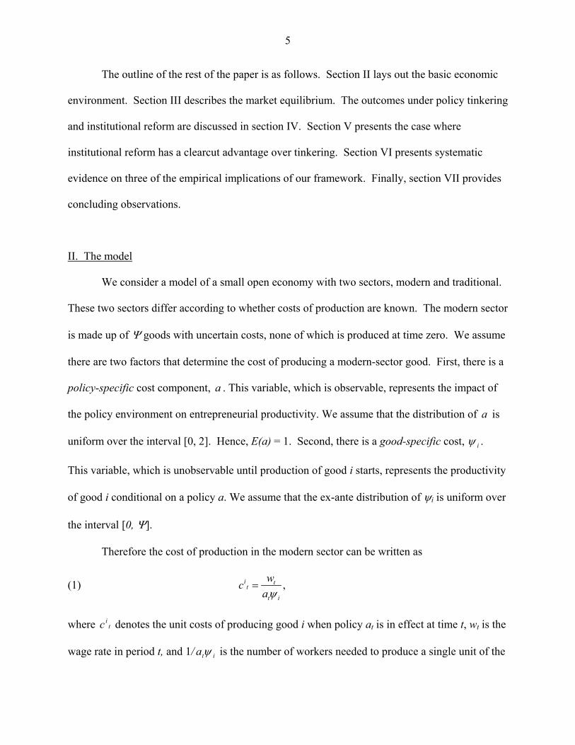
Therefore the cost of production in the modern sector can be written as
(1) ,it
tt
i
awcψ
=
where tic denotes the unit costs of producing good i when policy at is in effect at time t, wt is the
wage rate in period t, and 1/ ita ψ is the number of workers needed to produce a single unit of the

6
good i . Modern-sector production uses only labor and has constant-returns to scale technology
once productivity is known.
The justification for the uncertainty about costs of production in the modern sector is
provided by the fact that production involves learning along various different dimensions. For
instance, producing a good that has not been locally produced previously requires learning about
how to combine different inputs in a given environment, figuring out whether the existing local
conditions are conducive to efficient production, discovering the true costs of production, and so
on (see Hausmann and Rodrik 2003). In addition, our framework captures the idea that some
policy environments are better for entrepreneurship than others.
We note that the unobserved productivity parameters iψ is a property of individual
goods, and not of entrepreneurs: all entrepreneurs who run firms producing good i will operate
with productivity iψ .3 We shall assume that each modern-sector firm is of a given size, fixed
(by appropriate choice of units) to one unit of good i’s output. Each entrepreneur can run one,
and no more than one, modern-sector firm.
Discovering iψ requires setting up the firm and utilizing one unit of labor.4 Let mt
denote the number of entrepreneurs who choose to establish firms in period t, which also equals
the total amount of (sunk) labor investment in the same period. After firms are set up and labor is
sunk, iψ ’s become known for those mt goods in which investments have been made.
Subsequently, all mt entrepreneurs can produce a unit of the good and earn p (an exogenous price
3 Hence uncertainty is associated with costs of production rather than with entrepreneurial talents. Once an entrepreneur discovers costs in a given sector, there is a large number of entrepreneurs who can emulate the incumbent. Some other models of industrialization emphasize instead the selection of talented entrepreneurs who can best undertake the innovations needed for modern production. See for example Acemoglu, Aghion, and Zilibotti (2002). 4 One way of thinking of this is that all entrepreneurs are self-employed.

7
fixed on world markets5). During this inaugural production stage, which we call the “cost
discovery” phase, there is no entry into the modern sector so that any entrepreneur who draws a
cost less than or equal to p earns excess profits. (Even though p is fixed, so is output due to the
assumptions that firm size is fixed and an entrepreneur cannot run more than a single firm.) This
transitional period of monopoly profits can be motivated in one of two ways. It could be that it
takes time for the iψ to become common knowledge. Alternatively, iψ can be immediately
known, but it could take time for an “imitator” to set up a firm. Note that while some firms will
make profits in the cost-discovery phase, the ex-ante expected profits from starting a new firm
would be zero in equilibrium. This is because the quantity of entrepreneurship, mt, is determined
endogenously.
Following the cost-discovery phase, production in the modern sector enters the
“consolidation” phase, in which there is free entry into any pre-existing modern-sector activity
and excess profits are eliminated. The mechanism through which the latter happens is the
upward adjustments in the wage rate wt as labor is drawn toward the modern sector and modern-
sector production expands. Since there are no diminishing returns to labor in the modern sector,
we will have an extreme form of industry rationalization in this phase: all but the highest
productivity modern sector activity cease to exist.
The productivity of the modern sector in the consolidation phase is the maximum from
the mt draws made by entrepreneurs, which will be itself conditional on the policy rule in effect,
ta . Let this maximum productivity be denoted by )(maxtmψ . Since the ex-ante distribution of
iψ is uniform over [0, Ψ] and the draws are independent, the expected value of the rank statistic
5 Note that these are goods that are already being produced in other, more advanced countries. So saying that there are known, fixed prices is not at odds with the assumption that none of them is produced at home currently.
8
)(maxtmψ has the simple form E[ )(max
tmψ ] = Ψ mt/(1+ mt). Note that E[ )(maxtmψ ] is increasing
in mt but at a decreasing rate. We shall assume that entrepreneurs (as well as policy makers) are
risk neutral.
We close the model by describing production in the traditional sector. The traditional
sector operates under constant returns to scale and employs labor and a fixed factor. It will be
convenient to use a specific functional form, so we write the production function in the
traditional sector as yt = ( tsl − )α , where l is the total labor force of the economy, st is
employment in the modern sector, and α is the factor share of labor in the traditional sector. At
any given time t, total employment in the modern sector equals the sum of workers employed in
new entrepreneurial ventures (during the cost-discovery phase), mt,6 and the workers employed
in previously-established modern sector firms (during the consolidation phase), et. That is,
ttt ems += . The diminishing marginal returns to labor in the traditional sector implies that the
modern sector faces a positively sloped labor supply curve. Adjustments in wages will therefore
play an important equilibrating role for our economy. The price of the traditional sector is fixed
at 1 as the numeraire.
Economic activity extends over infinite discrete time. Every period t, t > 0, begins with
an inherited policy at-1 and a maximum known productivity in the modern sector max1−t
ψ drawn in
the preceding period. Then, on the basis of at-1 and max1−t
ψ , the policy maker can make one of the
following choices: (a) no new draw (status quo); (b) a new draw at from the existing policy
regime (policy tinkering); or (c) a new draw bt from a new policy regime (institutional reform).
Like policy draws from the existing regime, draws from a new policy regime are uniformly
6 Remember that we normalized the number of workers needed to start a new firm to 1.
9
distributed over the continuum [0, 2]. Hence E(b) = E(a) = 1.7 But institutional reform imposes a
cost on incumbent modern-sector activities, so that the productivity of the incumbent modern-
sector activity following a regime change is φ btmax
1−tψ with 0 < φ < 1, whereas that following
policy tinkering is equal to atmax
1−tψ .8
Within each time period, the complete sequence of events is as follows:
Stage 1: The government decides whether or not to make a new policy draw ta or
tb .
Stage 2: Conditional on the policy (either a newly drawn one or the one inherited
from the previous period), labor allocations (et≥ 0) and the new number of
entrepreneurs (mt ≥ 0) are determined.
Stage 3: Conditional on labor allocations and entrepreneurship decisions, wages
(wt) are determined. If tm > 0, new costs, iψ , are revealed. The highest
modern-sector productivity attains maxtψ . The market structure of any
young industry that has just emerged is one of monopoly, whereas that of
a pre-existing industry is characterized by free entry and a competitive
market.
7 More realistically, the policy experience of a country and the experience of other countries with similar socio-economic and geographic attributes may influence the range of the policy maker’s experimentation draws. For a discussion of the interplay between learning and policy experimentation, see Mukand and Rodrik (2002). Furthermore, there may be cases where institutional reform would yield a clearcut advantage over tinkering so that E(b) > E(a). We consider this case in Section V. 8 Of course, our qualitative results depend on a weaker form of this assumption: as long as incumbent firms bear higher adjustment costs when a new policy draw is made from a newly-instituted policy regime, our main results remain intact.

10
We proceed by first defining the equilibrium levels of entrepreneurial activity, labor
allocation and the determination of wages. We then explore the socially optimal patterns of
policy experimentation consistent with the market equilibrium.
III. Entrepreneurial activity, labor allocation and market equilibrium
We first note that in equilibrium et and mt cannot both be strictly positive. If it pays to
operate a pre-existing modern-sector activity with the highest known productivity, it will not pay
to start new entrepreneurial ventures with unknown productivity, and vice versa.
To see this, consider the relationship between the productivity of the incumbent modern-
sector activity and the expected productivity of entrepreneurship under both policy tinkering and
institutional reform. Under policy tinkering, suppose first that max1−t
ψ ≥ E (ψ ) = Ψ /2. Then, the
productivity of the most efficient pre-existing modern-sector activity—which will either be in or
have gone through its consolidation phase—is higher than the expected productivity of new
entrepreneurial ventures, and no one will find it optimal to experiment with new activities. In
this case, all individuals prefer to work either in the traditional sector or the pre-existing modern
sector (with the consequence that et > 0 and mt = 0). If on the other hand max1−t
ψ < E (ψ ) = Ψ /2,
the expected entrepreneurial productivity draw exceeds pre-existing productivity levels in the
modern sector, and in equilibrium et = 0 and mt > 0. A similar argument holds under
institutional reform. In particular, if φ max1−t
ψ ≥ E (ψ ) = Ψ /2, then the productivity of the most
efficient pre-existing modern-sector activity—despite the fact that it incurs an adjustment cost—
is higher than the expected productivity of new entrepreneurial ventures. This leads to et > 0 and
mt = 0. But if φ max1−t
ψ < E (ψ ) = Ψ /2, then the productivity of the most efficient modern-sector

11
activity after the reform is below the expected entrepreneurial productivity. Hence, in
equilibrium et = 0 and mt > 0.
Given the policy maker’s choice, the equilibrium wage rates can be derived easily. If
policy tinkering is chosen when max1−t
ψ ≥ E (ψ ) = Ψ /2, we have mt = 0, and wt and et are
determined by the following two equations:
(2) 1)( −−= αα tt elw ,
and
(2’) max1−= ttt paw ψ .
The first of these equations ensures zero profits in the modern sector while the second represents
labor market-equilibrium. If on the other hand, policy tinkering is done when max1−t
ψ < E (ψ ) =
Ψ /2, then et = 0, and wt and mt are determined by the following equations:
(3) 1)( −−= αα tt mlw ,
and
(3’) 2Ψ
= tt paw .
Equation (3) ensures expected profits are zero for entrepreneurial ventures in an ex ante sense,
since expected profits for any individual entrepreneur are given by tπ = Ψ
−t
t
awp 2 .9
If institutional reform is chosen when max1−t
φψ ≥ E (ψ ) = Ψ /2, we have mt = 0, and wt
and et are determined by equation (2) and
(4) max1−= ttt bpw ψφ .
12
If on the other hand, institutional reform is undertaken when max1−t
φψ < E (ψ ) = Ψ /2, then et = 0,
and wt and mt are determined by equation (3) and
(5) 2Ψ
= tt pbw .
As shown, at any point in time, the modern sector will be either in a cost discovery phase
or in a consolidation phase but not both. The productivity of the incumbent modern-sector
activity, together with the policy choice, determines which of these phases the modern sector will
be in. For sufficiently low levels of initial modern-sector productivity and prevailing wages,
entrepreneurial activity/self-discovery would not be crowded out. Not so when the incumbent
modern-sector productivity and wage rates are relatively high (in which case employment in the
incumbent modern-sector activity would fully crowd out entrepreneurship).
In what follows, we explore optimal policy choice. In doing so, we focus solely on a
second-best world where the policy maker has the same uncertainty about production costs as
private entrepreneurs do.10
IV. Optimal policy choice
At the beginning of each period t > 0, the policy maker observes the maximum
productivity draw of the previous period max1−t
ψ and, depending on the inherited policy draw at-1,
decides whether or not to make a new policy draw at or bt.
What is the policy maker’s optimal decision? The easiest case to consider is the one
where the inherited policy draw, at-1, exceeds its expected value, E(a) = 1. In that case, the
9 As we will elaborate below, our model generates an inverse relationship between entrepreneurial experimentation and the prevailing wage rates. For empirical evidence, refer to section VI. Also, see Iyigun and Owen (1998, 1999) for some related discussion. 10 For an analysis of the full-information case, see Hausmann and Rodrik (2003).

13
policy maker would choose to maintain the status quo under all circumstances we examine
below, as there is nothing to be gained in expected value terms by making a renewed draw.
Under the status quo, free entry reigns, all but the highest productivity firms close down, and
imitation—together with the wage adjustment mechanism that accompanies it—drives profits
from that activity down to zero.
Policy tinkering does not affect margin between old and new activities, and hence does
not influence the equilibrium level of cost discovery. But institutional reform can generate cost
discovery where policy tinkering would fail to do so since the former reduces productivity (and
wages) in pre-existing activities. As a consequence, depending on the productivity of the
incumbent modern sector activity, max1−t
ψ , and whether the policy maker chooses to tinker, at, or
reform, bt, there are three other cases to consider: (i) φψ 2/max1 Ψ≥−t so that wages are too high to
generate new entrepreneurial ventures even after major reforms are instituted; (ii) 2/max1 Ψ<−tψ
which implies that wages are low enough that tinkering with existing policies is sufficient to
entice new entrepreneurs; and (iii) 2/2/ max1 Ψ≥>Ψ −tψφ so that wages are too high to yield new
entrepreneurship under policy tinkering but they are low enough to entice entrepreneurs with
institutional reforms.
We now turn to an examination of each of these cases.
(i) φψ 2/max1 Ψ≥−t :
In this region, wages are too high to warrant new entrepreneurial experimentation. Thus,
labor is allocated between the traditional sector and the incumbent modern-sector activity only.
That is, mt = 0 and st = et > 0.
14
The equilibrium wage rate equates the marginal product of labor in the incumbent
modern-sector activity to that of labor in the traditional sector, as indicated by equations (2) and
(2’):
(6) ( ) 1max11
−
−− −==ααψ tttt elpaw .
Using (6), we can solve for the level of employment in period t:
(7) α
ψα −
−−
−=
11
max11 tt
t pale .
Thus, with a policy 1−ta in place, the aggregate output of the economy will be given by Yt ≡ yt +
pxt, where
(8) α
α
α
ψα −
−−
=−=
1
max11
)(tt
tt paely ,
and
(9)
−==
−
−−−−−−
α
ψαψψ
11
max11
max11
max11
tttttttt pa
laaex .
Now consider the outcome when the policy maker decides to tinker and make a new draw
ta in period t. With the new policy in effect, the productivity of the incumbent activity would
equal max1−tta ψ . And as implied by equation (7), this would lead to a change in the level of
employment in the incumbent modern-sector activity.11
11 As we stated above, the new policy draw would not yield any new entrepreneurial ventures, no matter how large
ta is: that is because ta shifts the productivity of actual and potential modern-sector activities in the same proportion, and does not affect their relative profitability.

15
Let )( aYE t ≡ )( ayE t + p )( axE t denote the expected level of aggregate output
associated with tinkering (i.e., a new policy draw ta ). Given that E( a ) = 1, we establish the
following:
(10) α
α
α
ψα −
−
=−=
1
max1
)()(t
tt pelayE ,
(11)
−==
−
−−−
α
ψαψψ
11
max1
max1
max1)(
ttttt p
leaxE .
Next consider the case where the policy maker decides in favor of institutional reform
and makes a policy draw tb . The equilibrium wage rate equates the marginal product of labor in
the incumbent modern-sector activity to that of labor in the traditional sector:
(6’) ( ) 1max1
−
− −==ααψφ tttt elbpw ,
Using (6’), we can solve for the level of employment in period t:
(7’) α
ψφα −
−
−=
11
max1tt
t bple
Let )( bYE t , )( bYE t ≡ )( byE t + p )( bxE t , denote the expected level of aggregate
output conditional on the policy regime change. Since E(b) = 1, we can establish the following:
(10’) α
α
α
φψα −
−
=−=
1
max1
)()(t
tt pelbyE ,
(11’)
−==
−
−−−
α
φψαφψφψ
11
max1
max1
max1)(
ttttt p
lebxE .
Note that if it were not optimal for the policy maker to change policy in period t, it would
also not be optimal to do so in any subsequent period, since the economic environment is
16
assumed to remain unchanged. This suggests that the present discounted welfare associated with
the status quo is given by Yt /(1-β) where β, 0 < β < 1, denotes the time discount factor.
If instead the policy maker were to tinker (and make a new policy draw ta ) in period t,
the outcome would be stochastic. From this period’s vantage point, the expected value of the
outcome in any subsequent period would be )( aYE t , regardless of whether the policy maker
makes additional draws down the line. This is due to the fact that, evaluated at ta = E( a ) = 1,
Yt+1( a =1) would equal )( aYE t . Thus, the present discounted welfare associated with a policy
change is equal to )( aYE t /(1−β). Based on the same argument, the present discounted welfare
associated with institutional reform is equal to )( bYE t /(1−β).
An examination of equations (8)-(11), (10’) and (11’) reveals that
(12) ββ −
>− 11
)( tt YaYE and
ββ −>
− 1)(
1)( bYEaYE tt .
Hence, when 11 <−ta and φψ 2/max1 Ψ≥−t , we find that the policy maker would—instead
of pursuing major reforms—just tinker with existing policies. This is due to the fact that
institutional reforms are costly and without new entrepreneurial experimentation they provide no
additional benefit over policy tinkering.
(ii) 2/max1 Ψ<−tψ :
In this case, equilibrium wages are low enough that there is new entrepreneurial
experimentation and employment in the incumbent modern-sector activity is driven to zero.
Thus, labor is allocated between the traditional sector and new entrepreneurship only. That is, et
= 0 and st = mt > 0.

17
The equilibrium wage rate equates the expected marginal product of new entrepreneurial
ventures to that of labor in the traditional sector, as in equations (3) and (3’):
(13) ( ) 11
2−− −=
Ψ=
αα tt
t mlpa
w ,
Using (13), we can solve for the equilibrium level of expected entrepreneurial ventures:
(14) αα −
−
Ψ
−=1
1
1
2
tt pa
lm .
With no change in policy, the aggregate output of the economy would equal E(Yt) ≡ yt + pE(xt),
where
(15) α
α
α α −
−
Ψ
=−=1
1
2)(t
tt pamly ,
(16) 2
)( 1Ψ
= −ttt amxE .
This is a case in which there is no uncertainty with respect to the output of the traditional
sector because no new policy draw is made and the number of new entrepreneurial ventures is
observable ex ante. In contrast, there is uncertainty about the output of the highest modern-sector
activity because, while the expected value of the economy-wide outcome of entrepreneurial
ventures equals E[ )(maxtmψ ] = Ψ mt/(1+ mt), it actual value is not observable ex ante.
At time t+1 free entry reigns, eliminating all but the highest productivity modern-sector
activity. Thus, the expected level of aggregate output in all future periods, E(Yt+1) ≡ E( 1+ty ) +
pE( 1+tx ), equals
(17) α
α
α α −
−++
+Ψ
=−=1
111
]1[)()(t
t
ttt m
mpa
elyE ,

18
(18)
+Ψ
−+
Ψ==
−
−
−−+
ααψ1
1
]1[1
)]}([{)(1
1max11
t
t
tt
ttttt m
mpa
lm
maamEaexE .
Now consider the outcomes when the policy maker decides to tinker and make a new
policy draw at. Since the expected value of the draw ta equals E( a ) = 1, both the equilibrium
wage rate and the number of entrepreneurs would exceed those given by (13) and (14)
respectively. With )( aYE t ≡ )( ayE t + p )( axE t denoting the level of aggregate output
associated with tinkering and the expected new policy draw, ta = E( a ) = 1, we can establish the
following:
(19) α
α
α α −
Ψ
=−=12)()(
pmlayE tt ,
(20) 2
)( Ψ= tt maxE .
At time t+1 free entry eliminates all except the highest productivity modern-sector
activity which ex ante attains E{a )]([max amψ } = Ψmt/(1+mt). Thus, the expected level of
aggregate output in all future periods, Yt+1( a =1) ≡ )1(1 =+ ayt + p )1(1 =+ axt , equals
(21) α
α
α α −
++
+Ψ
=−==1
11]1[)()1(
t
ttt m
mp
elay ,
(22)
+Ψ
−+
Ψ===
−
+
ααψ1
1
]1[1
)]}([{)1( max1
t
t
t
ttt m
mp
lm
mamEeax .
Instead, if the policy maker opts out for institutional reform and makes a new policy draw
bt, the equilibrium wage rate is determined by the following equation:
19
(13’) ( ) 1
2−
−=Ψ
=αα t
tt ml
pbw .
With (13’), we can derive the equilibrium level of entrepreneurship:
(14’) αα −
Ψ
−=1
1
2
tt pb
lm .
The output of the economy will be given by )( bYE t , )( bYE t ≡ )( byE t + p )( bxE t , where the
components )( byE t and )( bxE t are identical to equations (19) and (20), respectively. The
expected output of the economy in all subsequent periods will equal Yt+1(b=1) , Yt+1(b=1) ≡
)1(1 =+ byt + p )1(1 =+ bxt , where the output of the traditional and the modern sectors are given
by (21) and (22), respectively.
Based on equations (15) through (22), we can now state the following:
(23) β
ββ
ββ
β−
+>−
=+=
−=
+ +++
1])([
)(1
])1([)(
1])1([
)( 111 tt
tt
tt
YEYE
bYbYE
aYaYE .
In (23), the terms ])1([ 1 =+ aYtβ )1/( β− and )1/(])1([ 1 ββ −=+ bYt are equal to one
another. This is due to the fact that, subsequent to the initial period in which monopoly rents
accrue, the expected aggregate output of the economy would be equal under the two policy-
setting regimes.12 The terms )( aYE t and )( bYE t are also equal, because policy draws from
either regime generate the same amount of entrepreneurial experimentation. As a result, we
establish that the policy maker would just tinker with existing policies if 11 <−ta and
2/max1 Ψ<−tψ .
12 This simply follows from the fact that E(a) = E(b) = 1.
20
(iii) φψ 2/2/ max1 Ψ<≤Ψ −t :
In this case, wages are low enough to warrant entrepreneurial experimentation under a
reform, but they are not sufficiently low to generate it with policy tinkering. Thus, in order to
determine the appropriate course of action, the policy maker would need to compare the
expected aggregate output associated with institutional reform that we discussed in part (ii) with
the expected aggregate output associated with policy tinkering that we presented in part (i).
In this case, for sufficiently high values of β, the following inequality would hold:
(24) βββ
β−
>−
>−
=+ +
11)(
1])1([
)( 1 tttt
YaYEbYbYE
As we show in the appendix, we find that 11 <∀ −ta and φψ 2/2/ max1 Ψ<≤Ψ −t reform dominates
tinkering for a sufficiently forward-looking policy maker who has a relatively high β. However,
we cannot rule out the possibility of status quo for max1−tψ in the neighborhood of φ2/Ψ for a
shortsighted policy maker. The reason that the discount rate matters is this: under the status quo
as well as tinkering, there are gains in the current period from consolidation in the modern sector
as resources move from less profitable activities to the highest-productivity incumbent activity.
Institutional reform generates (expected) gains in the future from higher cost discovery, but does
so at the cost of giving up these current gains.
In sum, our results have the following implications. Policy tinkering dominates
institutional reform when existing policies leave something to be desired and the modern-sector
is pretty unproductive (i.e., for at-1 < 1 and 2/max1 Ψ<−tψ ). In this case, the prevailing wage rate
is low enough to entice new cost discovery even in the absence of institutional reform. Hence,
given the adjustment costs involved and the possible loss of gains that arise during the
consolidation phase in the modern sector, it would not be desirable to alter the economy’s

21
institutional arrangements. Similarly, policy tinkering dominates institutional reform when
existing policies are not terribly desirable but the modern sector is quite productive (i.e., for at-1
< 1 and φψ 2/max1 Ψ≥−t ). In this case, wages are high enough to stifle cost discovery even when
institutional reform is attempted. Thus, given the adjustment costs involved with institutional
reform and the absence of cost discovery gains, it is desirable to tinker with policies within the
existing institutional framework. In contrast, provided that a policy maker is sufficiently
forward-looking, institutional reform dominates policy tinkering when existing policies are
undesirable and the modern sector is only moderately productive (i.e., for at-1 < 1 and
φψ 2/2/ max1 Ψ<≤Ψ −t ). In this case, the prevailing wage rate is low enough to entice new
entrepreneurial experimentation under institutional reform, but too high to do so under policy
tinkering. Hence, it is socially desirable to bear the adjustment costs and explore alternative
institutional arrangements. These results are summarized in Table 1.
As the table shows, the expected impact on welfare (and economic performance) of
institutional reform varies with the quality of pre-existing policies and the initial productivity of
the modern sector. In our model, initial productivity is in turn determined by the inherited level
of entrepreneurial experimentation. Note that even when it is not the dominant strategy,
institutional reform can improve welfare in economies where the productivity of the modern
sector is not too high. The same cannot be said with respect to economies where the modern
sector is relatively productive; in those economies policy tinkering would enhance welfare but
institutional reform would undermine it. We shall test this idea in our empirical work below.

22
V. Institutional reforms with large productivity impact
We have assumed so far that the expected productivity impact of institutional reform is
no greater than that of policy tinkering (i.e., E(b) = E(a) = 1). We finally consider the
possibility that E(b) > E(a). This corresponds to a case where the policy regime can be
unambiguously improved because existing institutional arrangements are exceedingly weak.
Suppose therefore that E(b) = γ > 1. Τhe expected productivity of an incumbent modern sector
activity after a policy regime change now equals max1−tγφψ . Thus, whether the cost of adjustment
to a new policy regime change is high enough to offset the expected gain of a reform will be
crucial. If the expected productivity impact of institutional reform were fairly large so that
1≥γφ , then reform would not be costly on net to incumbent modern-sector activities. The
government would then want to undertake institutional reform as long as γ=<− )(1 bEat . If, on
the other hand, the expected productivity impact of a reform were only moderately large so that
1<γφ , incumbent modern sector activities would still suffer an expected loss—albeit a smaller
one than that in the previous section—as a result of institutional reform.
What this suggests is that when there is no new entrepreneurial experimentation (as in
part (i) in the previous section where φψ 2/max1 Ψ≥−t ), institutional reforms with relatively small
expected productivity gains (i.e., γ closer to one) will still be dominated by policy tinkering.
However, as long as wages are low enough to allow new cost discovery (as in parts (ii) and (iii)
above), institutional reform will now unambiguously dominate tinkering since incumbents are
displaced by new entrepreneurial ventures anyway. In this latter case, the adjustment costs that
incumbents would have incurred had they remained in business become irrelevant.
23
VI. Empirical evidence
The model we discussed above yields a rich range of empirical implications. However,
testing these implications directly is rendered difficult by the absence of internationally
comparable measures of entrepreneurship, which plays a key mediating role in our framework.
The ILO provides some patchy cross-national data on self-employment.13 In the absence of
better proxies, we used this data to construct an index of entrepreneurial intensity (ENTRAT),
which we compute by taking the ratio of self-employed individuals to total non-agricultural
employment. This ratio can be calculated for more than 50 countries around the year 1990, and
varies from a low of 5% in Sweden to a high of 58% in Nigeria. We recognize that ENTRAT
varies systematically with levels of development, so we will control for per-capita GDP in all our
regressions to guard against spurious results. See Table 2 for summary statistics and the
correlation matrix for the variables used below.
We use ENTRAT to test three of the implications of our model. First, our model implies
that entrepreneurial experimentation is inversely related to the prevailing level of modern-sector
labor costs. Second, economies with higher levels of entrepreneurship should generate more
productive modern-sector activities and therefore should experience higher rates of economic
growth subsequently. And third, institutional reforms should stimulate economic activity the
most in countries where prior levels of entrepreneurship have been too low to generate much
high-productivity activity (or more precisely, the economic impact of reforms should
monotonically decline in prior levels of entrepreneurship; see Table 1).
Columns (1)-(3) of Table 3 present our results on the first implication. Our measure of
modern-sector labor costs is average unit labor costs in manufacturing (ln ULC), which we
calculate by taking the ratio of wages to manufacturing value added per employee (both from the

24
ILO). Since ENTRAT is measured around 1990, we compute ln ULC as an average for 1985-
1989. As column (1) shows, ln ULC exerts a negative and statistically significant influence on
ENTRAT, even after controlling for per-capita GDP. Since labor costs are also related to the
price level (see Rodrik 1999), we control for cross-country differences in the price level for
consumption (ln PC) in column (2). In column (3), we add three regional dummies as additional
controls. The estimated coefficient of ln ULC remains negative and statistically significant with
both robustness checks. In addition, the fit of our most parsimonious specification, which
includes unit labor costs and per-capita income only, is remarkably high; its adjusted R-squared
is 0.75.14
One possible concern with the specifications in (1)-(3) is reverse causation. Perhaps we
are getting the effect of entrepreneurial intensity on labor costs, rather than vice versa. But
theoretically this reverse relationship is positively signed rather than negatively signed. So if
there is simultaneous-equation bias at play, it should work against us (that is, the bias is in the
direction of making the estimated coefficient less negative). Another potential concern involves
the fact that labor costs might be a reflection of labor market inflexibility and the costs of
formality (generating a source of omitted variable bias). Here too, the effect would have been a
positive relationship—the more institutionalized the labor market, the greater the escape into
self-employment—rather than the negative one that we find. In addition, Friedman et al. (2000)
present cross-country data on the shares of the informal sectors in economic activity—all of
which are from the late 1980s or early 1990s. Using these estimates as additional explanatory
variables, we reran the specifications in columns (1) through (3). Accounting for the shares of
13 These data are accessible at http://www.ilo.org (LABORSTA dataset, Table 2.d). 14 This R-squared refers to a conventional OLS regression, and not the robust regressions we report in Table 2.

25
the informal sector not only did not influence our main results but also yielded insignificant
coefficients on the shares of the informal sector.15
We next turn to the relationship between entrepreneurship and subsequent growth. In our
model, the higher is the inherited level of entrepreneurship mt-1, the higher is the productivity
reached in the modern sector max1−tψ . We shall proxy max
1−tψ with economic growth. In order to
enlarge our sample size (which was limited to 53 countries in the previous set of regressions), for
this exercise we first use regression (3) to generate a predicted value for ENTRAT for more than
80 countries (ENTRAThat). Regressions (4)-(6) show that ENTRAThat is robustly correlated
with subsequent growth during the 1990s. The first of these regressions (col. (4)) is a bare-bones
specification, to which we next add regional dummies (col. (5)) and a number of standard growth
determinants (fertility, male schooling, and government consumption, col. (6)). Hence, the
intensity of entrepreneurship—as predicted by labor costs, among other things—has a positive
and significant impact on the subsequent rates of growth.16
Our third and most ambitious set of tests relates to the interaction between institutional
reform and the pre-existing level of entrepreneurship in determining economic outcomes. In our
model, a high level of entrepreneurship mt-1 raises the (expected) productivity in the modern
sector max1−tψ , but also lowers the return to institutional reform (see Table 1). We now test this last
implication.
To code our institutional reform variable, we rely on Wacziarg and Welch (2003), who
have recently revised and updated the Sachs-Warner (1995) data set on the timing of major
15 Thus, we do not report these results here. 16 We also explored the results of an instrumental variables, GMM specification using our actual ENTRAT data (which consist of 53 country observations). While we do not report them here, these results were roughly similar to—but slightly weaker than—the ones we present below: ENTRAT had a positive impact on subsequent growth in the analogs of columns (4) through (6) and the association between ENTRAT and growth was statistically significant at the five or ten percent confidence level in two of the three specifications.

26
reforms. The original Sachs and Warner (1995) effort was aimed at identifying countries that
had opened up their economies to trade and the timing of these reforms. However, the Sachs-
Warner definition of trade reform is so broad and demanding (requiring adjustments in trade
policies, macroeconomic policies, and structural policies) that it is quite well suited for our
purposes (see Rodriguez and Rodrik 2001 for a discussion). Hence, in order to be classified as
“open,” a country needs to have not only suitably low levels of trade barriers, but it must also
have no major macroeconomic disequilibria (measured by the black-market premium for foreign
currency), it must not have a socialist economic system, and must not have an export marketing
board. Since ENTRAT is measured around 1990, we code our REFORM variable as a dummy
variable that takes the value of 1 if the country has undergone a Sachs-Warner-Wacziarg-Welch
reform between 1985 and 1994 (inclusive). Our dependent variable is the change in growth
between the 1990s and 1970s, ∆GROWTH. (We exclude the 1980s because of the pervasive
effects of the Latin American debt crisis during that decade.) Our model implies that REFORM
should have different effects on ∆GROWTH depending on the value of ENTRAT.
In column (7) we regress ∆GROWTH on REFORM, ENTRAT, per-capita GDP and a set
of regional dummies. Note that the estimated coefficient on REFORM is negative (with a t-
statistic around 1). This result reflects the disappointing outcome with institutional reforms in
the 1990s, as discussed in the introduction (see also Rodrik 2003). In the next column (8), we
interact REFORM with ENTRAT. The results are quite striking. The estimated coefficient on the
interaction term is negative and highly significant. In addition, once the interaction term is
included, the coefficient on REFORM turns positive and becomes statistically significant. So the
impact of institutional reform turns out to be dependent on the level of our proxy for
entrepreneurship. Those that benefited were the countries with very low levels of entrepreneurial

27
intensity. In column (9) we repeat the exercise in an instrumental-variables framework, to
alleviate concern about the possible endogeneity of ENTRAT. We use as our instruments the
determinants of ENTRAT used in column (3) and their interaction with REFORM. The results
are equally strong. Institutional reform had dramatically different effects depending on the pre-
existing levels of entrepreneurial intensity.
According to our results, institutional reform enhanced growth in countries where
prevailing entrepreneurial intensity fell short of a certain cutoff level, and reduced growth
elsewhere. Using the estimates of column (8), we find this cutoff value of ENTRAT to be 0.17
(=.0411/.2477). This corresponds to the median value in our sample, and is about the level
observed in Malaysia. The countries in our sample that undertook institutional reform and where
ENTRAT was below this level are South Africa, Tunisia, Trinidad and Tobago, Israel, and New
Zealand. The average for Latin American countries is substantially above this cutoff at 0.27.
Interestingly, India and China, two important cases of gradualist tinkering, were likely above this
cutoff as well. While we do not have a value for ENTRAT for either of these countries, India’s
ENTRAThat is 0.30, and China (for which we cannot compute ENTRAThat due to missing labor
cost data) would have had to have labor costs that are implausibly high (two orders of magnitude
higher than India’s) to fall below the 0.17 threshold. Hence this evidence suggests that both
countries were better off not having undertaken deep institutional reform a la Latin America.
Encouraging as they are for our model, these results are obviously contingent on the
reliability of our proxy for entrepreneurial intensity ENTRAT and are sensitive to the coding of
REFORM. We end this section by providing a somewhat different type of evidence that does not
rely on either of these variables. We simply focus on the experience in Latin America, where we
know significant amounts of structural reform took place in the late 1980s and early 1990s. As

28
an alternative to ENTRAT, we use productivity growth in the 1970-1980 period as a proxy for the
strength of the cost discovery process and the vibrancy of entrepreneurship. (We ignore the
1980s once again, due to the special circumstances related to the debt crisis.) As before, we take
the difference in the growth rates of GDP per capita between the 1990s and 1970s as a measure
of the impact of institutional reform.
Figure 1 shows that there is a strong negative correlation in Latin America between TFP
performance during the 1970s and ∆GROWTH (ρ = -0.72). Countries that were experiencing
rapid TFP growth in the 1970s (e.g. Brazil) reaped little gains in the 1990s, while those that had
poor TFP growth performance (e.g. Chile) improved their performance. In line with the
implications of our framework, the payoffs to institutional reform were greatest when it was
likely to induce a new wave of entrepreneurship, i.e. when the cost discovery process had run out
of steam. And they were lowest when productivity performance was already satisfactory.
VII. Concluding remarks
We argued in this paper that the interplay between policy choices and entrepreneurial
incentives provides an important key to understanding recent patterns of economic performance
around the world. The taxonomy we offer yields a rich set of normative and positive
implications.
On the normative side, we find that optimal policy choice is highly contingent on initial
conditions. When the quality of pre-existing policies is high, status quo is the dominant policy
choice regardless of the productivity level in the modern sector. But when the quality of pre-
existing policies leaves something to be desired, the optimal choice between policy tinkering and
institutional reform depends critically on the level of productivity reached in the modern sector.

29
And the relationship is not linear. Policy tinkering is the best choice when the modern sector is
either (a) unproductive or (b) highly productive, while institutional reform is the best choice
when (c) the productivity level is intermediate between these two. The reason is that only in case
(c) does institutional reform have a clear advantage over tinkering: that is the case where
institutional reform induces cost discovery while tinkering fails to do so. In case (a) tinkering is
enough to generate cost discovery, while in case (b) neither tinkering nor institutional reform is
able to do so.
Perhaps our most striking conclusion is a positive one: institutional reforms boost
economic activity in countries where entrepreneurial activity is languishing and they fail in
places where entrepreneurial attempts at cost discovery are relatively vibrant. The available
empirical evidence supports such a conditional relationship. Hence recognizing the interplay
between reforms and entrepreneurship may help resolve the puzzle of why institutional reforms
have worked in a handful of countries while failing in others.
Our framework provides additional subtle insights on reform strategies and new ways to
interpret recent experience with economic development. Consider for instance our results on
policy tinkering. We find that policy tinkering works best when existing policies are
demonstrably poor and the productivity of modern sector activities is extremely low. This seems
to characterize the experience of some of the growth superstars of the last two decades fairly
well. In particular, China (since 1978), India (since 1980), and Vietnam (since 1986) have
scored spectacular economic gains with changes in institutional arrangements that fall far short
of what most Western economists would have considered a prerequisite for success. In India, the
changes in policy during the 1980s were barely perceptible. And even the more ambitious
reforms of the 1990s are better described as gradualist tinkering than as deep institutional reform.
30
China and Vietnam made considerable strides towards building a market economy while keeping
the basic socialist institutional arrangements (including state ownership of key industries)
intact.17 All three countries started from a very low level, not just in terms of the market-
friendliness of their policies, but also in terms of the productivity of their economies. Policy
tinkering has a potentially very high return under these circumstances, as our model shows. But
as the model also indicates, not all tinkerers will succeed; what matters is the actual policy draw.
Our model provides as well a reason for why Chinese-style gradualism may not have
worked in the former socialist countries of Eastern Europe, and therefore rationalizes the deeper
institutional reform and “shock therapy” that countries such as Poland and the Czech Republic
undertook. Unlike China and Vietnam, Eastern European countries had built modern
manufacturing sectors and were already high-wage economies. Tinkering would likely not have
been enough to generate new entrepreneurship and structural change. The fact that economic
performance in the former Soviet Union and Eastern Europe has turned out quite uneven is of
course once again consistent with one of our central building blocks—the uncertainty with
regard to policy outcomes.
We close by reiterating the central normative messages of this paper. Productive
transformation and policy reform are both subject to a great deal of uncertainty.
Entrepreneurship depends both on good policy and on adequate rents. Policy tinkering and
institutional reform both have their respective advantages. Appropriate strategies depend on
initial conditions, namely the quality of policies, the level of productivity in non-traditional
activities, and the state of entrepreneurship. Reformers who internalize these lessons are likely
to make good choices while those who don’t are likely to be disappointed.
17 See Rodrik and Subramanian (2004), Qian (2003) and van Arkadie and Mallon (2003) on India, China, and Vietnam, respectively.
31
APPENDIX
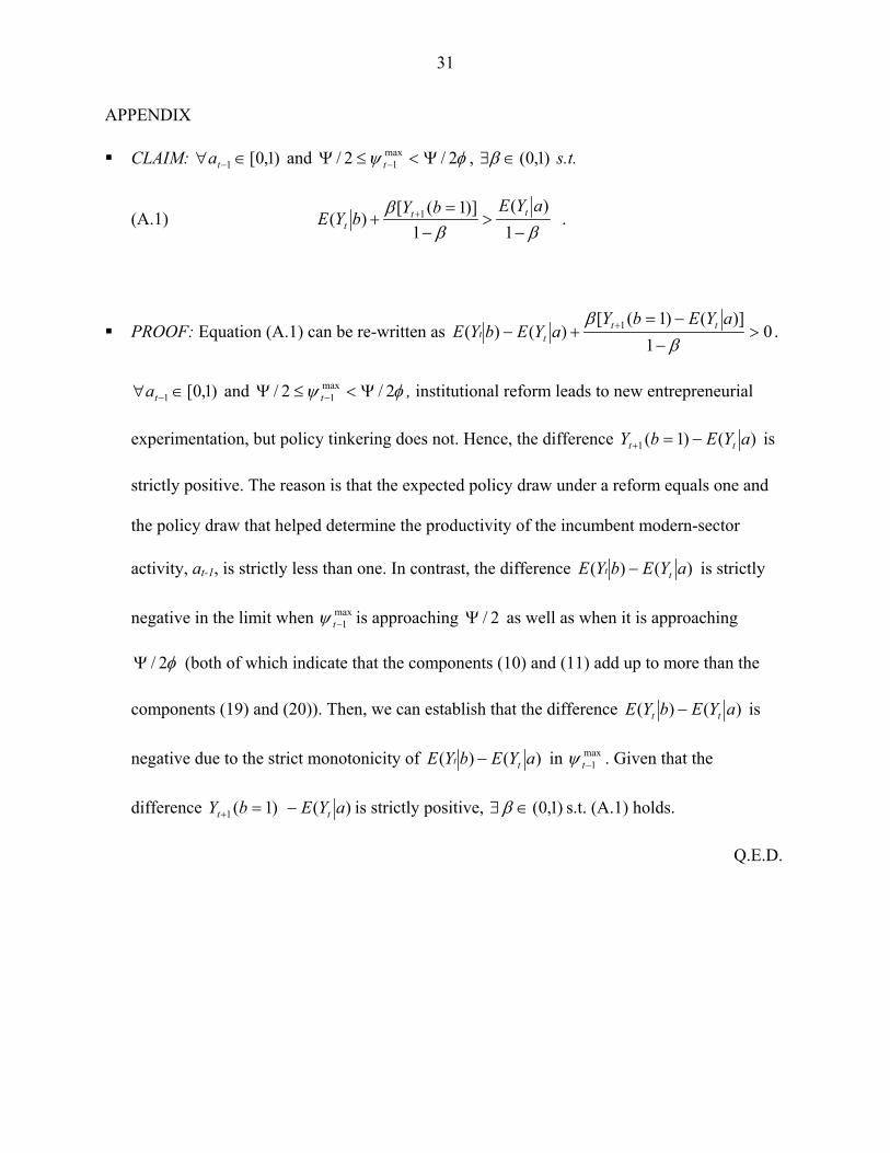
CLAIM: )1,0[1 ∈∀ −ta and φψ 2/2/ max1 Ψ<≤Ψ −t , )1,0(∈∃β s.t.
(A.1) ββ
β−
>−
=+ +
1)(
1])1([
)( 1 aYEbYbYE tt
t .
PROOF: Equation (A.1) can be re-written as 01
)]()1([)()( 1 >
−
−=+− +
ββ aYEbY
aYEbYE tttt .
)1,0[1 ∈∀ −ta and φψ 2/2/ max1 Ψ<≤Ψ −t , institutional reform leads to new entrepreneurial
experimentation, but policy tinkering does not. Hence, the difference )()1(1 aYEbY tt −=+ is
strictly positive. The reason is that the expected policy draw under a reform equals one and
the policy draw that helped determine the productivity of the incumbent modern-sector
activity, at-1, is strictly less than one. In contrast, the difference )()( aYEbYE tt − is strictly
negative in the limit when max1−tψ is approaching 2/Ψ as well as when it is approaching
φ2/Ψ (both of which indicate that the components (10) and (11) add up to more than the
components (19) and (20)). Then, we can establish that the difference )()( aYEbYE tt − is
negative due to the strict monotonicity of )()( aYEbYE tt − in max1−tψ . Given that the
difference )1(1 =+ bYt )( aYE t− is strictly positive, ∃ β )1,0(∈ s.t. (A.1) holds.
Q.E.D.

32
REFERENCES Acemoglu, Daron, Phillipe Aghion, and Fabrizio Zilibotti, “Distance to Frontier, Selection, and Economic Growth,” NBER Working Paper No. 9066, July 2002. Blanchard, Olivier, and Michael Kremer, “Disorganization,” Quarterly Journal of Economics, vol. 112, no. 4, 1997, 1091-1126. Bosworth, Barry, and Susan M. Collins, “The Empirics of Growth: An Update,” Brookings Institutions, unpublished paper, March 7, 2003. Caballero, Ricardo J., and Mohammed L. Hammour, “Creative Destruction and Development: Institutions, Crises, and Restructuring,” NBER Working Paper No. 7849, August 2000. Friedman, Eric, Simon Johnson, Daniel Kaufmann, and Pablo Zoido-Lobaton, “Dodging the Grabbing Hand: The Determinants of Unofficial Activity in 69 Countries,” Journal of Public Economics, June 2000. Harberger, Arnold C., “Interview with Arnold Harberger: Sound Policies Can Free Up Natural Forces of Growth,” IMF Survey, International Monetary Fund, Washington, DC, July 14, 2003, 213-216. Hausmann, Ricardo, and Dani Rodrik, “Economic Development as Self-Discovery,” Journal of Development Economics, December 2003. International Labor Organization, http://www.ilo.org, LABORSTA dataset, Table 2.d. Imbs, Jean, and Romain Wacziarg, “Stages of Diversification,” American Economic Review, 93(1), March 2003, 63-86. Iyigun, Murat F., and Ann L. Owen, “Risk, Entrepreneurship and Human Capital Accumulation,” American Economic Review (Papers & Proceedings), 88(2), May 1998, 454-57. Iyigun, Murat F., and Ann L. Owen, “Entrepreneurs, Professionals, and Growth,” Journal of Economic Growth, 4(2), June 1999, 211-30. Mukand, Sharun, and Dani Rodrik, “In Search of the Holy Grail: Policy Convergence, Experimentation, and Economic Performance,” NBER Working Paper 9134, August 2002. Qian, Yingyi, “How Reform Worked in China,” in D. Rodrik, ed., In Search of Prosperity: Analytic Narratives of Economic Growth, Princeton, NJ, Princeton University Press, 2003. Rodriguez, Francisco, and Dani Rodrik, “Trade Policy and Economic Growth: A Skeptic’s Guide to the Cross-National Evidence,” NBER Macroeconomics Annual, eds. Ben Bernanke and Kenneth S. Rogoff, MIT Press, Cambridge, MA, 2001.
33
Rodrik, Dani, “Democracies Pay Higher Wages,” Quarterly Journal of Economics, August 1999. Rodrik, Dani, “Growth Strategies,” Handbook of Economic Growth, eds. Philippe Aghion and Steven Durlauf, (forthcoming), mimeograph, September 2003. Rodrik, Dani, and Arvind Subramanian, “From ‘Hindu Growth’ to Productivity Surge: The Mystery of the Indian Growth Transition,” Harvard University, March 2004. Roland, Gerard, and Thierry Verdier, “Transition and the Output Fall,” Economics of Transition, vol. 7, no. 1, 1999, 1-28. Sachs, Jeffrey, and Andrew Warner, “Economic Convergence and Economic Policies,” Brookings Papers on Economic Activity, eds. William Brainard and George Perry, 1:1995, 1-95, 108-118. Van Arkadie, Brian, and Raymond Mallon, Vietnam: A Transition Tiger?, Asia Pacific Press at The Australian National University, Australia, 2003. Wacziarg, Romain, and Karen Horn Welch, “Trade Liberalization and Growth: New Evidence,” work in progress, November 2003.

Table 1. Summary of main implications Quality of pre-existing policies:
lousy (at-1 < 1) good (at-1 ≥ 1) low
productivity max
1−tψ < Ψ /2
intermediate productivity
φψ 2/2/ max1 Ψ<≤Ψ −t
high productivity
max1−tψ ≥ φ2/Ψ
low productivity
max1−tψ < Ψ /2
High productivity
max1−tψ ≥ 2/Ψ
optimal policy tinker inst. reform tinker status quo Status quo cost discovery under optimal policy?
yes yes no yes no
expected impact on welfare of
tinkering: + + + + + + + + + + - inst reform: + + + + + + + + + + / - - - policy ranking tinker
inst ref s.q.
inst ref tinker
s.q
tinker s.q.
inst. ref
status quo tinker inst ref

35
Table 2. Descriptive statistics
Correlation Matrix Mean S.D. GROWTH ENTRAT lnULC lnPC lnGDPCAP FERT SECM REF. ∆GRW GOVT GROWTH .0151 .0209 1.00 … … … … … … … … ENTRAT .188 .109 -.278 1.00 … … … … … … … ln ULC -1.126 .4375 -.042 -.680 1.00 … … … … … … ln PC -.675 .381 -.100 -.612 .513 1.00 … … … … … ln GDPCAP 8.38 1.13 .208 -.838 .607 .747 1.00 … … … … FERT 1.53 2.07 -.260 .691 -.509 -.609 -.915 1.00 … … … SECM 4.98 8.03 .158 -.502 .399 .609 .604 -.577 1.00 … … REFORM .355 .481 -.420 -.175 .510 -.330 -.476 .475 -.391 1.00 … ∆GRW -.0084 .0277 .372 .008 -.116 -.079 .012 -.158 .139 -.175 1.00 GOVT 7.35 9.26 -.048 .126 .045 -.258 -.455 .486 -.155 .037 .116 1.00

36
Table 3. Main results
(1) (2) (3) (4) (5) (6) (7) (8) (9) Dependent Variable: ENTRAT Dependent Variable: GROWTH Dependent Variable: ∆GROWTH OLS OLS OLS OLS OLS OLS OLS OLS IV
ln ULC -.0481* (.0137)
-.0514* (.0143)
-.0412* (.015)
…
…
…
… … …
ln GDPCAP -.0842* (.0067)
-.0884* (.0092)
-.0635* (0.0087)
.0124* (.0027)
.021* (.0079)
.0181* (.0077)
-.0112 (.0077)
-.0108 (.0069)
-.0196** (.0086)
ln PC …
.0165 (.0207)
-.0362*** (.0193)
… …
…
… … …
ENTRAT …
…
…
… … … -.0847 (.0579)
-.0143 (.0552)
-.1197** (.064)
ENTRAThat … … … .1098* (.0359)
.2284* (.0916)
.2151* (.0892)
… … …
LAAM … … .0279** (.013)
…
-.0155* (.0061)
-.0119** (.0060)
-.0039 (.0100)
-.0033 (.0093)
-.0019 (.008)
SAFRICA … … -.1032* (.0154)
…
.0096 (.0124)
.0118 (.0119)
-.0239*** (.0133)
-.0646* (.0122)
-.0566* (.012)
ASIA … … -.0030 (.0153)
…
.0090 (.0071)
.0137** (.007)
-.0162 (.0105)
-.0165*** (.0093)
-.0191* (.005)
SECM … … …
…
…
-.0001 (.0003)
… … …
FERT … … …
…
…
-.0008 (.0018)
… … …
GOVT … … …
…
…
.0006 (.0004)
… … …
REFORM
… … … … … …
-.0089 (.009)
.0411* (.016)
.0351** (.018)
REFORM* ENTRAT
… … … … … … … -.2477* (.0719)
-.1912** (.086)
Observations: 53 52 52 82 82 81 53 53 50 Note: Robust regression estimates, except for col. (9) which shows IV-GMM estimates. GROWTH is per-capita GDP growth from 1990 to
2000. ∆GROWTH is the difference between growth rate in the 1990s and growth rate in the 1970s. See text for more details. Standard errors in parentheses. * significant at 1 %; ** significant at 5 %, *** significant at 10 % .

37
Figure 1: Relationship between prior productivity growth and impact of institutional reform in Latin America
ARG
BOL
BRA
CHL
COL
CRI
DOM
ECU
GTMHND
MEX
PER
PGY
SLV
UGY
VEN
-10
-50
5D
iffer
ence
in g
row
th in
GD
P p
er w
orke
r, 19
90s
vs 1
970s
-4 -2 0 2 4TFP grow th 1970-80
Source: Data on TFP and GDP per worker from Bosworth and Collins (2003)