Net Present Value Analysis

Avinash Kishore(avinash.kishore@gmail.com)

Based on Notes from Andrew Foss

February 04, 2011Review Section

Agenda

Fundamental Theories of Welfare Economics

Static Efficiency

Dynamic Efficiency (NPV)

Internal Rate of Return

Equivalent Annual Net Benefits

Readings on Benefit-Cost Analysis

Practice Problem(s)

Excel Workbook Embedded Here:

2

Microsoft Office Excel 97-2003 Worksheet

Fundamental Theories of Welfare Economics:Pareto Criterion and Pareto Optimality

Pareto Criterion: A policy change is an improvement if at least some people are made better off and no one is made worse off

Pareto Optimality: No other feasible policy could make at least one person better off without making anyone else worse off

3Adam’s Payment

Beth’s Payment

StatusQuo

Policy A

Policy B

Policy C

Policy D

Feasibility Frontier

Possible Payments to Adam and Beth Which satisfy Pareto Criterion?

‒ Policy A does ‒ Policy B does not‒ Policy C does not‒ Policy D does‒ All policies in light gray triangle

Which satisfy Pareto Optimality?

‒ Policy A does not ‒ Policy B does not‒ Policy C does‒ Policy D does‒ All policies on feasibility frontier (because nothing “better” from there)

$25 $100

$25

$100

Fundamental Theories of Welfare Economics:Kaldor-Hicks Criterion

Kaldor-Hicks Criterion: A policy change is an

improvement if the “winners” could fully compensate the

“losers” and still be better off themselves

– Also known as Potential Pareto Improvement Criterion

Kaldor-Hicks Criterion rules out policies with total

benefits smaller than total costs (that is, policies with

negative net benefits, where NB = TB - TC)

When the Kaldor-Hicks Criterion is used to compare all

feasible policy options, the best is that which maximizes

net benefits

– If all policies have negative net benefits, keep the status quo4

0

5

10

15

20

25

0 1 2 3 4 5 6 7 8 9 10

Ma

rgin

al B

en

efi

ts o

r M

arg

ina

l Co

sts

Quantity of Pollution Control

0

20

40

60

80

100

120

0 1 2 3 4 5 6 7 8 9 10

To

tal B

en

efi

ts o

r T

ota

l C

os

ts

Quantity of Pollution Control

Static Efficiency (Single time period)

Undertake policy to the point at which TB – TC is the

highest

marginal benefit = marginal cost

5

Total Benefits

Total Costs

Marginal Benefits

Marginal CostsNet Benefits

Q*

Total Benefits and Total Costs Marginal Benefits and Marginal Costs

Q*

Dynamic Efficiency: when B and C in different time periods

To achieve dynamic efficiency (multiple time periods),

undertake policy with highest net present value

If all policies have negative NPV, keep the status quo

Discount rate should reflect social opportunity cost

U.S. Office of Management and Budget (OMB)

published guidance on discount rate and benefit-cost

analysis in Circular A-4 (September 2003):http://www.whitehouse.gov/omb/assets/regulatory_matters_pdf/a-4.pdf

6

T

tttt

r

CB

0 )1(NPV

OMB Guidelines on C-B Analysis

“For transparency’s sake, you should state in your

report what assumptions were used, such as the time

horizon for the analysis and the discount rates

applied to future benefits and costs.

It is usually necessary to provide a sensitivity analysis

to reveal whether, and to what extent, the results of

the analysis are sensitive to plausible changes in the

main assumptions and numeric inputs”.

7

Why do we need discounting? (Circular A4, OMB)

Benefits or costs that occur sooner are generally more

valuable– Resources invested earn a positive return, so current consumption is more

expensive than future consumption, since you are giving up that expected

return on investment when you consume today. (Opportunity Cost).

– Postponed benefits also have a cost because people generally prefer

present to future consumption. (Positive time preference).

– Also, if consumption continues to increase over time, as it has for most of

U.S. history, an increment of consumption will be less valuable in the future

than it would be today (Principle of diminishing marginal utility).

8

What is the appropriate discount rate?

“a real discount rate of 7 percent should be used as a

base-case for regulatory analysis”.

Why?

– “The 7 percent rate is an estimate of the average before-tax

rate of return to private capital in the U.S. economy.

– the returns to real estate and small business capital as well as

corporate capital.

– It approximates the opportunity cost of capital

– it is the appropriate discount rate whenever the main effect of

a regulation is to displace or alter the use of capital in the

private sector”.

9

The appropriate discount rate ?

The effects of regulation do not always fall exclusively or primarily

on the allocation of capital.

When regulation primarily and directly affects private

consumption (e.g., through higher consumer prices for goods and

services), a lower discount rate is appropriate.

The alternative most often used is sometimes called the social

rate of time preference

…the rate at which society discounts future consumption flows to

their present value. – the rate that the average saver uses to discount future consumption as a

measure

Real rate of return on long-term government debt ( = 3%)

10

How does discounting work?

Reciprocal of compounding

Benefits and costs far in the future are more sensitive to discount

rate than near-term benefits and costs

– Run discounting program in Excel workbook

11

r = 3% → NPV = $29M r = 10% → NPV = -$10M

-$250

-$200

-$150

-$100

-$50

$0

$50

$100

0 1 2 3 4 5 NPV

Net

Ben

efit

s (m

illi

on

s)

Undiscounted Net Benefits Discounted Net Benefits

-$250

-$200

-$150

-$100

-$50

$0

$50

$100

0 1 2 3 4 5 NPV

Net

Ben

efit

s (m

illi

on

s)

Undiscounted Net Benefits Discounted Net Benefits

How does discounting work?

When costs are incurred up front and benefits occur in

the future, low discount rates result in higher NPVs than

high discount rates

12

Relationship between Discount Rate and NPVwith Upfront Costs and Future Benefits

-$50

-$40

-$30

-$20

-$10

$0

$10

$20

$30

$40

$50

0% 2% 4% 6% 8% 10% 12% 14% 16% 18% 20%

Net

Pre

sen

t V

alu

e (m

illio

ns)

r

Dynamic Efficiency:Power Plant Example

You are a special assistant to Gov. Schwarzenegger of

California. He wants to shut down a coal-fired power plant

and replace it with either a hydropower plant or a natural gas-

fired plant. He asks you to analyze the options.

Assumptions (unrealistic…)

– Both plants can be built in 1 year and operate for 5 years

– Both plants yield annual benefits of $50M relative to coal

– Hydropower plant has upfront fixed costs of $100M and

annual operating costs of $5M

– Natural gas plant has upfront fixed costs of $40M and

annual operating costs of $20M

– Discount rate is 7 percent, but also try 3 and 10 percent

13

Dynamic Efficiency:Power Plant Example

Hydropower has a slightly higher NPV than natural gas

at 7 percent discount rate, but lower at 10 percent

14

$0

$20

$40

$60

$80

$100

$120

r = 3% r = 7% r = 10%

Ne

t Pre

se

nt

Va

lue

(m

illio

ns

)

Hydropower Natural Gas

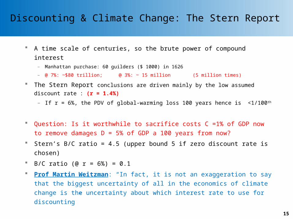
Discounting & Climate Change: The Stern Report

A time scale of centuries, so the brute power of compound interest– Manhattan purchase: 60 guilders ($ 1000) in 1626

– @ 7%: ~$80 trillion; @ 3%: ~ 15 million (5 million times)

The Stern Report conclusions are driven mainly by the low assumed discount

rate : (r = 1.4%)

– If r = 6%, the PDV of global-warming loss 100 years hence is <1/100 th

Question: Is it worthwhile to sacrifice costs C =1% of GDP now to

remove damages D = 5% of GDP a 100 years from now?

Stern’s B/C ratio = 4.5 (upper bound 5 if zero discount rate is chosen)

B/C ratio (@ r = 6%) = 0.1

Prof Martin Weitzman: “In fact, it is not an exaggeration to say that the

biggest uncertainty of all in the economics of climate change is the

uncertainty about which interest rate to use for discounting”

15

Health related costs and benefits

Question: is discounting even appropriate?

– lives saved today cannot be invested in a bank to save more

lives in the future.

Answer: Yes!

– People have been observed to prefer health gains that occur

immediately to identical health gains that occur in the future.

– If future health gains are not discounted while future costs

are, then what happens?

– an attractive investment today in future health improvement

can always be made more attractive by delaying the

investment

16

Internal Rate of Return:Overview

Internal rate of return answers the question, “What

discount rate would make NPV zero?”

When costs are incurred up front and benefits occur in

the future, undertake project if IRR > r

In the first discounting example (p. 7), IRR ≈ 8 percent

Internal rate of return is less robust than NPV, and it

should not be used to rank projects when constraints

make it impossible to undertake them all

17

0)1(

NPV0

T

tt

tt

IRR

CB

Internal Rate of Return:Power Plant Example

A nuclear power plant can be built in 1 year for $100M, can operate

for 5 years, yields annual benefits of $55M relative to coal, has

annual operating costs of $5M, and has decommissioning costs of

$155M in Year 6

18-$6

-$5

-$4

-$3

-$2

-$1

$0

$1

$2

$3

0% 2% 4% 6% 8% 10% 12% 14% 16% 18% 20%

Net

Pre

sen

t V

alu

e (m

illio

ns)

r

IRR??

IRR is not useful in this case because there are costs in the future

Equivalent Annual Net Benefits

Suppose the hydropower plant replacing the coal plant

in California can operate for 10 years and the natural

gas plant can still only operate for 5 years

– At r = 7 percent, NPVhydro = $216M and NPVgas = $83M

– At r = 32* percent, NPVhydro = $32M and NPVgas = $30M

* This is an unusually high discount rate, but it illustrates the point for the example numbers

Calculate equivalent annual net benefits to compare

these projects of different duration

– At r = 7 percent, EANBhydro = $27M and EANBgas = $16M

– At r = 32 percent, EANBhydro = $8M and EANBgas = $9M 19

Trr

rNPVEANB

)1(1

Readings on Benefit-Cost Analysis:Arrow et al. (1996)

Benefit-cost analysis is a important framework for

making regulatory decisions

– Careful consideration of benefits and costs

– Common unit of measurement for disparate impacts (dollars)

– Useful tool for improving effectiveness of regulation

– Techniques for incorporating uncertainty

But benefit-cost analysis should not be the sole basis

for making regulatory decisions

– Consideration of distributional impacts as well

– Perhaps not necessary to perform benefit-cost analysis for

minor regulations

20

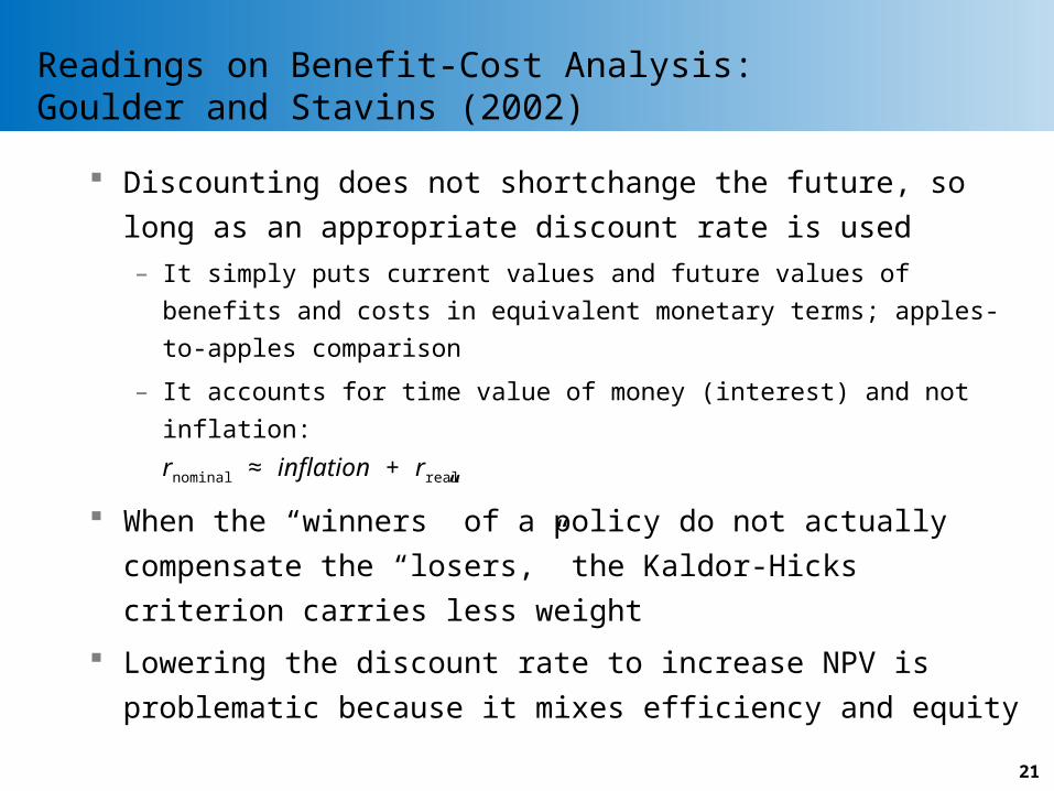
Readings on Benefit-Cost Analysis:Goulder and Stavins (2002)

Discounting does not shortchange the future, so long as

an appropriate discount rate is used

– It simply puts current values and future values of benefits and

costs in equivalent monetary terms; apples-to-apples

comparison

– It accounts for time value of money (interest) and not inflation:

rnominal ≈ inflation + rreal

When the “winners” of a policy do not actually

compensate the “losers,” the Kaldor-Hicks criterion

carries less weight

Lowering the discount rate to increase NPV is

problematic because it mixes efficiency and equity 21

Practice Problem: Coase Theorem

22

Private Goods and Public Goods:Beekeeper and Farmer Example

A beekeeper and a farmer are neighbors. The bee-

keeper’s bees help pollinate the farmer’s orchard.

The beekeeper’s marginal benefit from Q beehives is

MBbeekeeper(Q) = 10 – Q

The beekeeper’s marginal cost is constant at

MCbeekeeper(Q) = 7

The farmer’s marginal benefit from Q beehives is

MBfarmer(Q) = 5 – Q

If the beekeeper ignores impacts on the orchard, how

many beehives will the beekeeper have? What if the beekeeper takes impacts on the orchard into account?

23

Private Goods and Public Goods:Beekeeper and Farmer Example

If the beekeeper treats the beehives as a private good,

the beekeeper will have 3 beehives

24

0

5

10

15

0 5 10 15

MB

or

MC

Quantity of Beehives

MB_beekeeper MC_beekeeper

Q*

MCbeekeeper

MBbeekeper = MCbeekeeper

10 – Q = 7

Q* = 3 beehives

MBbeekeeper

0

5

10

15

0 5 10 15

MB

or

MC

Quantity of Beehives

MB_beekeeper MC_beekeeper MB_farmer MB_society

Private Goods and Public Goods:Beekeeper and Farmer Example

If the beekeeper treats the beehives as a public good,

the beekeeper will have 4 beehives

– Public goods are underprovided by private decision-making

25

Q*

MBbeekeeper

MCbeekeeper

MBsociety = MBbeekeeper + MBfarmer

(vertical sum of MBs for public goods)

For 0 ≤ Q ≤ 5 (where both MBs ≥ 0),

MBsociety = (10 – Q) + (5 – Q) = 15 – 2Q

MCsociety = MCbeekeeper

MBsociety = MCbeekeeper

15 – 2Q = 7

Q* = 4 beehives

MBsociety

MBfarmer

Private Goods and Public Goods:Beekeeper and Farmer Example

If the beekeeper and farmer can negotiate without

transaction costs, what outcome would we expect?

26

Increasing the number of beehives from 3 to 4 gives the

beekeeper extra benefits of $6.50 (area under MBbeekeeper)

but extra costs of $7 (area under MCbeekeeper), so the

beekeeper’s profit decreases by $0.50

Increasing the number of beehives from 3 to 4 gives the

farmer extra benefits of $1.50 (area under MBfarmer) and

does not impose extra costs on the farmer

By the Coase Theorem, the farmer could give the bee-

keeper between $0.50 and $1.50 to have 4 beehives