Neural Network-Based Genetic Job Assignment for … Network-Based Genetic Job Assignment for Automated Guided Vehicles Auftragsvergabe basierend auf mit genetischen Algorithmen trainierten

Neural Network-Based Genetic Job Assignment for Automated Guided Vehicles

Auftragsvergabe basierend auf mit genetischen Algorithmen trainierten neuronalen Netzen für Fahrerlose Transportsysteme

Paolo Pagani Dominik Colling

Kai Furmans

Institut für Fördertechnik und Logistiksysteme (IFL) Karlsruher Institut für Technologie (KIT)

utomated guided vehicles are designed to autono-

mously transport material in production and ware-

house environments. The loading/unloading process of

the material on the vehicles occurs at dedicated stations,

called material sources and destinations. Every time a ve-

hicle is idle, a new transportation job, i.e. the transporta-

tion of some goods from a material source to a material

destination, can be assigned to one of the vehicles, which

represents the limiting resource. The policies, which are

used for the job assignment, are several. In this paper, a

new policy based on neural networks which were trained

by genetic algorithms is proposed and evaluated. The re-

sults show that this new policy outperforms a policy

which is a combination of the so called “First Come First

Served” and the “Nearest Vehicle First” policy.

[Keywords: Automated guided vehicles, AGV, job assignment,

neural networks, genetic algorithms]

ahrerlose Transportsysteme werden häufig für den

innerbetrieblichen Materialtransport im Produkti-

ons- und Lagerumfeld genutzt. Die Be- und Entladung

mit Material findet an bestimmten Stationen, den Quellen

und Senken, statt. Transportaufträge führen immer von

einer Quelle zu einer Senke. Diese werden den Fahrzeu-

gen, die die begrenzte Ressource im System darstellen, zu-

geordnet. Dafür gibt es unterschiedliche Verfahren. In

dieser Veröffentlichung wird ein neues Verfahren vorge-

stellt und evaluiert, das auf von genetischen Algorithmen

trainierten neuronalen Netzen basiert. Die Versuche zei-

gen, dass das vorgestellte Verfahren bessere Ergebnisse

liefert als ein Verfahren, das eine Kombination aus „First

Come First Served“- und dem „Nearest Vehicle First“-

Verfahren darstellt.

[Schlüsselwörter: Fahrerlose Transportsysteme, FTS, Auftrags-

vergabe, neuronale Netze, genetische Algorithmen]

1 INTRODUCTION

Due to shorter product life cycles and an increasing

number of product variants, manufacturers are increasingly

demanding greater flexibility. At the same time, a more

cost-effective production is necessary due to rising cost

pressure. While automation and flexibility were contradict-

ing terms in the past, they must now coexist. Through ad-

vanced developments in sensor and in safety technology,

nowadays driverless transport systems can achieve both

goals. Thus, a further spread of AGVs (or automated

guided vehicles) can be expected in the future. With the aid

of laser scanners, those driverless vehicles can navigate

freely in facilities and warehouses, so that the required in-

frastructure is significantly reduced. As one example, the

installation of induction loops is no longer necessary. This

saves installation costs and makes a change of the layout

even during operation possible. Furthermore, AGVs can

work around the clock with a high level of availability and

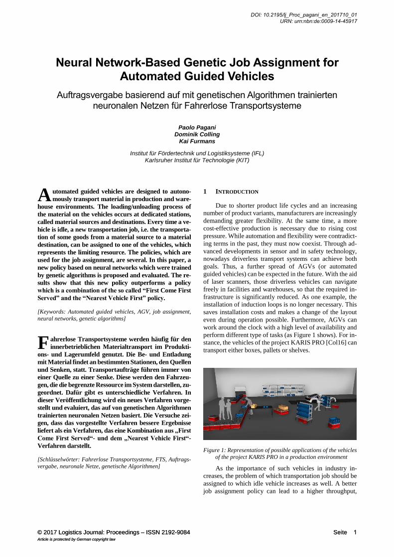
perform different type of tasks (as Figure 1 shows). For in-

stance, the vehicles of the project KARIS PRO [Col16] can

transport either boxes, pallets or shelves.

Figure 1: Representation of possible applications of the vehicles

of the project KARIS PRO in a production environment

As the importance of such vehicles in industry in-

creases, the problem of which transportation job should be

assigned to which idle vehicle increases as well. A better

job assignment policy can lead to a higher throughput,

A

F

© 2017 Logistics Journal: Proceedings – ISSN 2192-9084 Seite Article is protected by German copyright law

1© 2017 Logistics Journal: Proceedings – ISSN 2192-9084 Seite Article is protected by German copyright law

1

DOI: 10.2195/lj_Proc_pagani_en_201710_01 URN: urn:nbn:de:0009-14-45917

lower operating costs and/or a lower number of required

vehicles.

This is why we have developed a new job assignment

policy which is based on neural networks which have been

trained by genetic algorithms.

This research paper is organized as follows: In section

2 the standard job assignment methods are discussed. In

section 3 we will explain how the system has been mod-

elled. In section 4 we will describe how the neural network

works and how it is trained. In section 5 we will carry out

a case study. Finally, we will describe the conclusions in

section 6.

2 JOB ASSIGNMENT POLICIES

Automated guided vehicles, shortly AGVs, are un-

manned transportation systems that are designed to auton-

omously transport goods within production and warehouse

environments. Their loading and unloading process on the

vehicles occurs at dedicated stations (see Figure 2), which

will be denoted in this paper as material sources and mate-

rial destinations. In particular, a material source is a station

where goods, denoted as material units, arrive from the up-

stream part of the production or logistic chain and need to

be delivered by an AGV to a certain material destination to

proceed in the logistical chain. On the contrary, a material

destination is a station where the material units must be de-

livered. As a result, the goal of AGVs is to pick up the ma-

terial units from material sources and bring them to the cor-

respondent material destinations. For each transport, these

two tasks are summarized in a job and before the execution

of a job, it has to be assigned to a vehicle.

Figure 2: Dedicated stations for the autonomous loading and un-

loading process of the material units (KARIS PRO concept)

According to [Arn08], we can distinguish between two

different kinds of job assignment to a vehicle: preplanning

and dispatching.

Preplanning means assigning a job as soon as it is gen-

erated. The advantage of this method is that you can plan

already early with the implications of a job assignment like

vehicle utilization. It is often used when you have to aggre-

gate several jobs to one tour. This is why it is usually used

for LTL transports and not for AGVs.

Dispatching means that a job gets only allocated when

a vehicle gets idle. A job assignment takes place either if a

job has been newly generated and there is at least one idle

vehicle or if a vehicle terminates a job and there are further

not-allocated jobs. Due to this latest possible decision the

newest network conditions can be taken into account when

making an assignment. Dispatching is usually used for

AGVs as the network conditions are often changing and in

contrast to LTL a job assignment is very extensive as one

job occupies a whole vehicle. This is why we will focus on

dispatching.

According to [LeA06] dispatching rules for AGVs can

be separated in two groups: Single-attribute and multi-at-

tribute dispatching rules. Single attribute dispatching rules

base their assignment decision on only one attribute. They

can be classified into three groups. Time-based dispatching

rules try to minimize the throughput time of each job. For

example, considering the First Come First Served Policy,

the idle AGV chooses to transport the material unit, which

is waiting the longest amount of time in the material source.

Workload-based dispatching rules are for example

used in production environments where you have several

machines and workstations which have to be supplied with

materials. The rules try to keep all sources receptive for

new material and try to provide all workstations sufficient

material. This is why this policy always chooses the source

with least free stations and/or the destination with most free

stations.

Distance-based dispatching rules try to minimize the

travelled distances of the vehicles. This is why, using this

policy, an idle AGV always chooses to transport the mate-

rial unit, which is closest to itself.

In some situations, these single attribute dispatching

rules perform poorly, since they are limited to only one ob-

jective which can be effective in some situations but not in

all of them. This is why often multi- attribute dispatching

rules are used. They base their decisions on several attrib-

utes.

In literature, many more job assignment policies can

be found. Meta-heuristic strategies [Abd14] have been de-

veloped and applied in many scheduling problems, e.g.

project scheduling or job shop scheduling. They have gen-

erally outperformed the heuristic ones in most of the cases

[Leu15] by finding good solutions with less computational

effort [Blu03]. One of the most promising group of meta-

heuristic algorithms are the neural network-based strate-

gies, like for example [Fen03], [Foo88] and [Par00]. They



2


are able to link the current system state to the decision to

be taken with very complex relations, which are very diffi-

cult to be described by means of heuristic rules and which

are identified by topology, the weights and thresholds of

the neural network itself. As a result, they perform well in

comparison to other heuristic and meta-heuristic methods,

when the relations between the current system state and the

best decision are complex and not intuitive. Moreover,

those strategies can also be combined with other heuristics

or meta-heuristics [Hai01].

In this paper, the combination between a neural net-

work-based policy and a genetic algorithm, in a similar way

to the one applied to the project scheduling in [Aga11], has

been proposed and tested to design a neural network-based

decision tool for the job assignment of AGVs.

3 SYSTEM MODELLING

In this section, it is explained how the problem under

investigation is modelled. The model is composed by four

main modelling objects: material units, material sources,

material destinations and vehicles. For instance, Figure 3

represents an example of system composed by two material

sources, two material destinations and two vehicles.

The material units (in Figure 3 depicted as full squares

and denoted by the letter “M”) represent some group of

goods, which can be identified by a common container or

carrier, for example a box, a transportable shelf or a pallet.

They are supplied from the upstream part of the logistic

chain to the material sources. Once they lay on the material

source, the AGVs are in charge to bring them to the right

material destination. Once they lay on one of the material

destinations, they can be withdrawn to continue in the

downstream part of the logistic chain.

The material sources (in Figure 3 depicted as empty

squares and denoted by the letters “MS” followed by a

number) are dedicated stations where the material units

constantly arrive with an arrival process described by a

Gaussian distributed interarrival time. Those stations are

also characterized by a maximum number of buffer places

and by (x,y) coordinates in a 2D layout. When a new mate-

rial unit is about to arrive and all buffer places are busy (see

MS2 in Figure 3), it is assumed that this material unit does

not enter the considered system. As a result, each material

unit that cannot be delivered to a material source contrib-

utes to lower the total system throughput, which is the ob-

jective function of the model.

The material destinations (in Figure 3 depicted as

empty squares and denoted by the letters “MD” followed

by a number) are dedicated stations where the material

units are constantly withdrawn with a withdrawal process

described by a Gaussian distributed interdeparture time. As

for the material sources, those stations are also character-

ized by a maximum number of buffer places and by (x,y)

coordinates in a 2D layout. When a material unit is required

to be withdrawn at a material destination and no material

unit are available in it (see MD1 in Figure 3), it is assumed

that that demand is lost. As a result, each material unit that

cannot be withdrawn from a material destination also con-

tributes to lower the total system throughput.

Finally, the vehicles are the AGVs to which the trans-

portation jobs, i.e. the transportation of a material unit from

one material source to one material destination, can be as-

signed. Once they have completed a transportation job,

they wait in an idle state at the material destination where

they have delivered the last transported material unit. They

represent the limiting resource, i.e. the higher their number,

the higher the throughput, if the saturation has not been

reached yet and if there are no blocking effects due to high

traffic. They are characterized by the moving speed and a

loading/unloading time, i.e. an additional time that is re-

quired to perform the loading/unloading process of the ma-

terial unit on the vehicle, e.g. fine positioning, load transfer,

etc.

Figure 3: Example of system with two material sources (four

buffer places each), two material destinations (four buffer

places each) and two vehicles.

The dispatching of the material is defined by a dis-

patching matrix DM, whose element 𝐷𝑀𝑖,𝑗 identifies the

probability that a material unit arriving at the material

source i must be delivered at the material destination j. As

a result, it has a number of rows equal to the number of

material sources and a number of columns equal to the

number of material destinations. In the case depicted in

Figure 3, where each material source is coupled to a mate-

rial destination, the dispatching matrix is as follows:

DM = [1 00 1

]



3


4 STRUCTURE OF THE NEURAL NETWORK-BASED

GENETIC ALGORITHM

In this section, it is explained how the neural network-

based genetic algorithm works. In particular, it is described

how a neural network can be used as a decision tool for the

job assignment and how it can be trained without training

samples by using a genetic algorithm.

4.1 NEURAL NETWORK AS DECISION TOOL

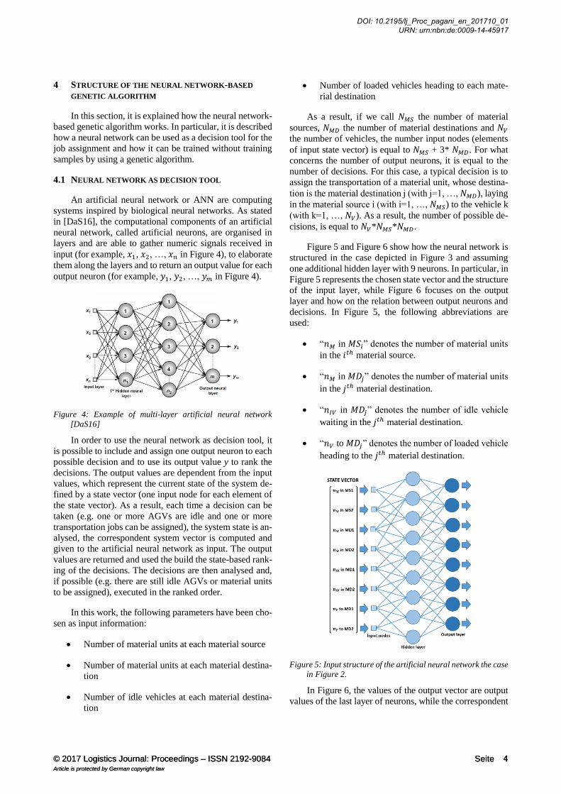
An artificial neural network or ANN are computing

systems inspired by biological neural networks. As stated

in [DaS16], the computational components of an artificial

neural network, called artificial neurons, are organised in

layers and are able to gather numeric signals received in

input (for example, 𝑥1, 𝑥2, …, 𝑥𝑛 in Figure 4), to elaborate

them along the layers and to return an output value for each

output neuron (for example, 𝑦1, 𝑦2, …, 𝑦𝑚 in Figure 4).

Figure 4: Example of multi-layer artificial neural network

[DaS16]

In order to use the neural network as decision tool, it

is possible to include and assign one output neuron to each

possible decision and to use its output value y to rank the

decisions. The output values are dependent from the input

values, which represent the current state of the system de-

fined by a state vector (one input node for each element of

the state vector). As a result, each time a decision can be

taken (e.g. one or more AGVs are idle and one or more

transportation jobs can be assigned), the system state is an-

alysed, the correspondent system vector is computed and

given to the artificial neural network as input. The output

values are returned and used the build the state-based rank-

ing of the decisions. The decisions are then analysed and,

if possible (e.g. there are still idle AGVs or material units

to be assigned), executed in the ranked order.

In this work, the following parameters have been cho-

sen as input information:

Number of material units at each material source

Number of material units at each material destina-

tion

Number of idle vehicles at each material destina-

tion

Number of loaded vehicles heading to each mate-

rial destination

As a result, if we call 𝑁𝑀𝑆 the number of material

sources, 𝑁𝑀𝐷 the number of material destinations and 𝑁𝑉

the number of vehicles, the number input nodes (elements

of input state vector) is equal to 𝑁𝑀𝑆 + 3* 𝑁𝑀𝐷. For what

concerns the number of output neurons, it is equal to the

number of decisions. For this case, a typical decision is to

assign the transportation of a material unit, whose destina-

tion is the material destination j (with j=1, …, 𝑁𝑀𝐷), laying

in the material source i (with i=1, …, 𝑁𝑀𝑆) to the vehicle k

(with k=1, …, 𝑁𝑉). As a result, the number of possible de-

cisions, is equal to 𝑁𝑉*𝑁𝑀𝑆*𝑁𝑀𝐷.

Figure 5 and Figure 6 show how the neural network is

structured in the case depicted in Figure 3 and assuming

one additional hidden layer with 9 neurons. In particular, in

Figure 5 represents the chosen state vector and the structure

of the input layer, while Figure 6 focuses on the output

layer and how on the relation between output neurons and

decisions. In Figure 5, the following abbreviations are

used:

“𝑛𝑀 in 𝑀𝑆𝑖” denotes the number of material units

in the 𝑖𝑡ℎ material source.

“𝑛𝑀 in 𝑀𝐷𝑗” denotes the number of material units

in the 𝑗𝑡ℎ material destination.

“𝑛𝐼𝑉 in 𝑀𝐷𝑗” denotes the number of idle vehicle

waiting in the 𝑗𝑡ℎ material destination.

“𝑛𝑉 to 𝑀𝐷𝑗” denotes the number of loaded vehicle

heading to the 𝑗𝑡ℎ material destination.

Figure 5: Input structure of the artificial neural network the case

in Figure 2.

In Figure 6, the values of the output vector are output

values of the last layer of neurons, while the correspondent



4


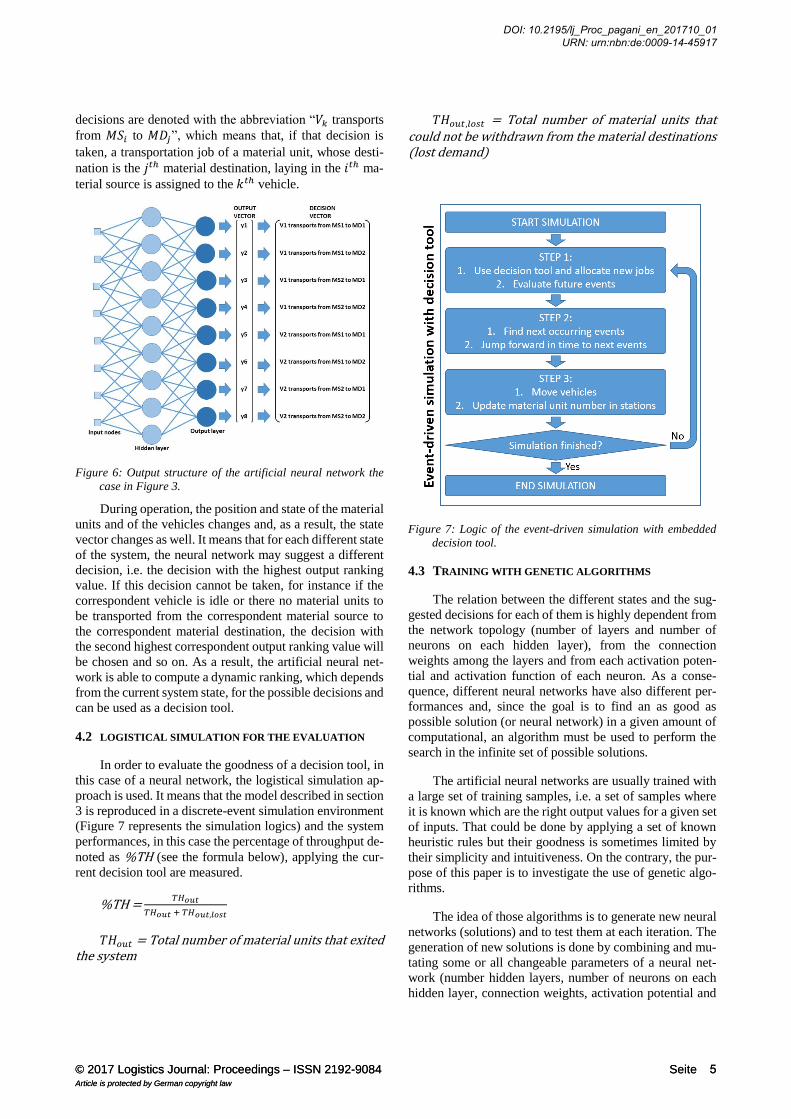
decisions are denoted with the abbreviation “𝑉𝑘 transports

from 𝑀𝑆𝑖 to 𝑀𝐷𝑗”, which means that, if that decision is

taken, a transportation job of a material unit, whose desti-

nation is the 𝑗𝑡ℎ material destination, laying in the 𝑖𝑡ℎ ma-

terial source is assigned to the 𝑘𝑡ℎ vehicle.

Figure 6: Output structure of the artificial neural network the

case in Figure 3.

During operation, the position and state of the material

units and of the vehicles changes and, as a result, the state

vector changes as well. It means that for each different state

of the system, the neural network may suggest a different

decision, i.e. the decision with the highest output ranking

value. If this decision cannot be taken, for instance if the

correspondent vehicle is idle or there no material units to

be transported from the correspondent material source to

the correspondent material destination, the decision with

the second highest correspondent output ranking value will

be chosen and so on. As a result, the artificial neural net-

work is able to compute a dynamic ranking, which depends

from the current system state, for the possible decisions and

can be used as a decision tool.

4.2 LOGISTICAL SIMULATION FOR THE EVALUATION

In order to evaluate the goodness of a decision tool, in

this case of a neural network, the logistical simulation ap-

proach is used. It means that the model described in section

3 is reproduced in a discrete-event simulation environment

(Figure 7 represents the simulation logics) and the system

performances, in this case the percentage of throughput de-

noted as %TH (see the formula below), applying the cur-

rent decision tool are measured.

%TH = 𝑇𝐻𝑜𝑢𝑡

𝑇𝐻𝑜𝑢𝑡 + 𝑇𝐻𝑜𝑢𝑡,𝑙𝑜𝑠𝑡

𝑇𝐻𝑜𝑢𝑡 = Total number of material units that exited the system

𝑇𝐻𝑜𝑢𝑡,𝑙𝑜𝑠𝑡 = Total number of material units that could not be withdrawn from the material destinations (lost demand)

Figure 7: Logic of the event-driven simulation with embedded

decision tool.

4.3 TRAINING WITH GENETIC ALGORITHMS

The relation between the different states and the sug-

gested decisions for each of them is highly dependent from

the network topology (number of layers and number of

neurons on each hidden layer), from the connection

weights among the layers and from each activation poten-

tial and activation function of each neuron. As a conse-

quence, different neural networks have also different per-

formances and, since the goal is to find an as good as

possible solution (or neural network) in a given amount of

computational, an algorithm must be used to perform the

search in the infinite set of possible solutions.

The artificial neural networks are usually trained with

a large set of training samples, i.e. a set of samples where

it is known which are the right output values for a given set

of inputs. That could be done by applying a set of known

heuristic rules but their goodness is sometimes limited by

their simplicity and intuitiveness. On the contrary, the pur-

pose of this paper is to investigate the use of genetic algo-

rithms.

The idea of those algorithms is to generate new neural

networks (solutions) and to test them at each iteration. The

generation of new solutions is done by combining and mu-

tating some or all changeable parameters of a neural net-

work (number hidden layers, number of neurons on each

hidden layer, connection weights, activation potential and



5


activation function), as they were genes of a DNA. As a

result, it is possible to move in the solution space by gener-

ating new solutions.

The genetic algorithm for neural network-based deci-

sion tools proposed in this paper works as follows:

1. Initialize the algorithm parameters:

a. Define a maximum number of generated neural

networks, i.e. solutions, (computational con-

straint). This parameter is denoted as 𝑁𝑚𝑎𝑥 .

b. Define an initial population size of the solu-

tions. This parameter is denoted as 𝑁𝑝.

c. Define a number of generated combined solu-

tions, i.e. a number of solutions that are created

by combining random preexisting solutions at

each iteration. This parameter is denoted as 𝑁𝑐.

d. Define a number of generated mutated solu-

tions, i.e. a number of solutions that are created

by mutating random preexisting solutions at

each iteration. This parameter is denoted as 𝑁𝑚.

e. Define the topology of the neural networks

(number of layers and number of neurons on

each hidden layer). The topology is kept fixed

for all the generated solutions. The number of

input nodes and output neurons is based on the

number of parameters of the input vector and to

the number of possible decisions.

2. Generate the initial population of 𝑁𝑝 solutions.

3. Add 𝑁𝑐 combined solutions to the population. A

combined solution is obtained by randomly

choosing 2 parent solutions and by transferring

some parameters of the neural network from one

parent solution and some from the other.

4. Add 𝑁𝑚 mutated solutions to the population. A

mutated solution is obtained by randomly choos-

ing one parent solution. Some parameters of the

neural network are transferred from the parent so-

lution, while others are randomly mutated.

5. Evaluate the goodness of the “𝑁𝑝+𝑁𝑐+𝑁𝑚” indi-

viduals (neural networks) of the population as de-

cision tool for the job assignment in the event-

driven simulation environment.

6. Remove the worst performing neural networks

and kept only the best 𝑁𝑝 ones.

7. If the number of total generated neural networks

(initial + combined + mutated) is lower than

𝑁𝑚𝑎𝑥 , repeat from step 3, else stop algorithm.

5 CASE STUDY

In this section, a case study is presented to test and

compare the neuro-genetic algorithms on a concrete exam-

ple.

5.1 CASE INTRODUCTION

In the considered system, five material sources and

five material destinations are considered. We have 1:1 con-

nections so that each material source has its own material

destination. The positions of the stations and the corre-

spondent material destinations for each material source are

represented in Figure 8 by the layout and the dashed ar-

rows. It is considered an interarrival and interdeparture

time equal to 120 seconds on average, a standard deviation

of 30 for all stations and five buffer places for each of them.

The system is served by four vehicles with a speed of 1 m/s

and a loading/unloading time, i.e. an extra time required to

autonomously load and unload the vehicles with the mate-

rial units.

Figure 8: Representation of the system considered in the case

study

For what concerns the genetic algorithm used to gen-

erate new neural networks, the following parameters have

been assumed:



6


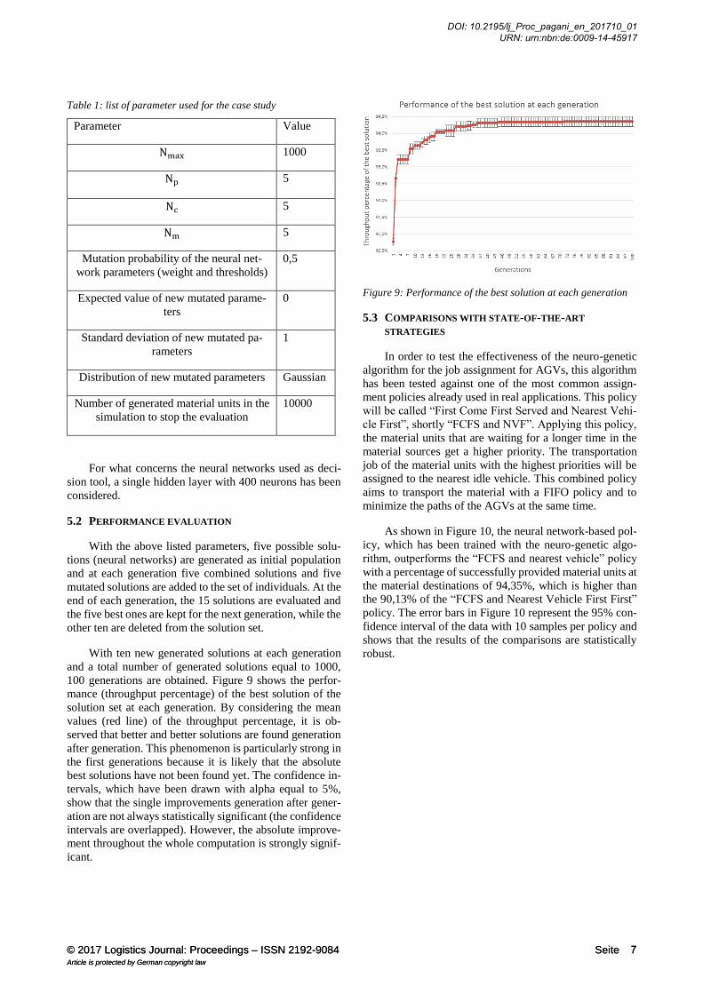
Table 1: list of parameter used for the case study

Parameter Value

Nmax 1000

Np 5

Nc 5

Nm 5

Mutation probability of the neural net-

work parameters (weight and thresholds)

0,5

Expected value of new mutated parame-

ters

0

Standard deviation of new mutated pa-

rameters

1

Distribution of new mutated parameters Gaussian

Number of generated material units in the

simulation to stop the evaluation

10000

For what concerns the neural networks used as deci-

sion tool, a single hidden layer with 400 neurons has been

considered.

5.2 PERFORMANCE EVALUATION

With the above listed parameters, five possible solu-

tions (neural networks) are generated as initial population

and at each generation five combined solutions and five

mutated solutions are added to the set of individuals. At the

end of each generation, the 15 solutions are evaluated and

the five best ones are kept for the next generation, while the

other ten are deleted from the solution set.

With ten new generated solutions at each generation

and a total number of generated solutions equal to 1000,

100 generations are obtained. Figure 9 shows the perfor-

mance (throughput percentage) of the best solution of the

solution set at each generation. By considering the mean

values (red line) of the throughput percentage, it is ob-

served that better and better solutions are found generation

after generation. This phenomenon is particularly strong in

the first generations because it is likely that the absolute

best solutions have not been found yet. The confidence in-

tervals, which have been drawn with alpha equal to 5%,

show that the single improvements generation after gener-

ation are not always statistically significant (the confidence

intervals are overlapped). However, the absolute improve-

ment throughout the whole computation is strongly signif-

icant.

Figure 9: Performance of the best solution at each generation

5.3 COMPARISONS WITH STATE-OF-THE-ART

STRATEGIES

In order to test the effectiveness of the neuro-genetic

algorithm for the job assignment for AGVs, this algorithm

has been tested against one of the most common assign-

ment policies already used in real applications. This policy

will be called “First Come First Served and Nearest Vehi-

cle First”, shortly “FCFS and NVF”. Applying this policy,

the material units that are waiting for a longer time in the

material sources get a higher priority. The transportation

job of the material units with the highest priorities will be

assigned to the nearest idle vehicle. This combined policy

aims to transport the material with a FIFO policy and to

minimize the paths of the AGVs at the same time.

As shown in Figure 10, the neural network-based pol-

icy, which has been trained with the neuro-genetic algo-

rithm, outperforms the “FCFS and nearest vehicle” policy

with a percentage of successfully provided material units at

the material destinations of 94,35%, which is higher than

the 90,13% of the “FCFS and Nearest Vehicle First First”

policy. The error bars in Figure 10 represent the 95% con-

fidence interval of the data with 10 samples per policy and

shows that the results of the comparisons are statistically

robust.



7


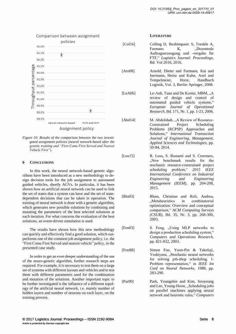
Figure 10: Results of the comparison between the two investi-

gated assignment policies (neural network-based after the

genetic training and “First Come First Served and Nearest

Vehicle First”).

6 CONCLUSIONS

In this work, the neural network-based genetic algo-

rithms have been introduced as a new methodology to de-

sign decision tools for the job assignment to automated

guided vehicles, shortly AGVs. In particular, it has been

shown how an artificial neural network can be used to link

the set of states that a system can have and the set of state-

dependent decisions that can be taken in operation. The

training of neural network is done with a genetic algorithm,

which generates new possible solutions by combining and

mutating the parameters of the best selected solutions at

each iteration. For what concerns the evaluation of the best

solutions, an event-driven simulation is used.

The results have shown how this new methodology

can quickly and effectively find a good solution, which out-

performs one of the common job assignment policy, i.e. the

“First Come First Served and nearest vehicle” policy, in the

presented case study.

In order to get an even deeper understanding of the use

of the neuro-genetic algorithm, further research steps are

required. For example, it is necessary to test them on a large

set of systems with different layouts and vehicles and to test

them with different parameters used for the combination

and mutation of the solutions. Another important topic to

be further investigated is the influence of a different topol-

ogy of the artificial neural network, i.e. mainly number of

hidden layers and number of neurons on each layer, on the

training process.

LITERATURE

[Col16] Colling D, Ibrahimpasic S, Trenkle A,

Furmans K, „Dezentrale

Auftragserzeugung und -vergabe für

FTF,“ Logistics Journal: Proceedings,

Bd. Vol 2016, 2016.

[Arn08] Arnold, Dieter and Furmans, Kai and

Isermann, Heinz and Kuhn, Axel and

Tempelmeier, Horst, Handbuch

Logistik, Vol. 3, Berlin: Springer, 2008.

[LeA06] Le-Anh, Tuan and De Koster, MBM, „A

review of design and control of

automated guided vehicle systems,“

European Journal of Operational

Research, Bd. 171, Nr. 1, pp. 1-23, 2006.

[Abd14] M. Abdolshah, „A Review of Resource-

Constrained Project Scheduling

Problems (RCPSP) Approaches and

Solutions,“ International Transaction

Journal of Engineering, Management,

Applied Sciences and Technologies, pp.

50-84, 2014.

[Leu15] R. Leus, S. Rostami and S. Creemers,

„New benchmark results for the

stochastic resource-constrained project

scheduling problem,“ 2015 IEEE

International Conference on Industrial

Engineering and Engineering

Management (IEEM), pp. 204-208,

2015.

[Blu03] Blum, Christian and Roli, Andrea,

„Metaheuristics in combinatorial

optimization: Overview and conceptual

comparison,“ ACM Computing Surveys

(CSUR), Bd. 35, Nr. 3, pp. 268-300,

2003.

[Fen03] S. Feng, „Using MLP networks to

design a production scheduling system,“

Computers and Operations Research,

pp. 821-832, 2003.

[Foo88] Simon Foo, Yoon-Pin & Takefuji,

Yoshiyasu, „Stochastic neural networks

for solving job-shop scheduling. I-

Problem representation,“ in IEEE Int

Conf on Neural Networks, 1988, pp.

283-290.

[Par00] Park, Youngshin and Kim, Sooyoung

and Lee, Young-Hoon, „Scheduling jobs

on parallel machines applying neural

network and heuristic rules,“ Computers



8


and Industrial Engineering, pp. 189-

202, 2000.

[Hai01] Haibin Yu, Wei Liang, „Neural network

and genetic algorithm-based hybrid

approach to expanded job-shop

scheduling,“ Computers & Industrial

Engineering, Bd. 39, Nr. 3, pp. 337-356,

2001.

[Aga11] Anurag Agarwal, Selcuk Colak, Selcuk

Erenguc, „A Neurogenetic approach for

the resource-constrained project

scheduling problem,“ Computers &

Operations Research, Bd. 38, Nr. 1, pp.

44-50, 2011.

[DaS16] Da Silva, Ivan Nunes and Spatti, Danilo

Hernane and Flauzino, Rogerio Andrade

and Liboni, Luisa Helena Bartocci and

dos Reis Alves, Silas Franco, Artificial

Neural Networks: A Practical Course,

Springer, 2016.

M.Sc. Paolo Pagani is working as a Research Assistant at

the chair of Robotics and Assistance Systems, Institute of

Material Handling and Logistics (IFL), Karlsruhe Insti-

tute of Technology (KIT).

E-Mail: [email protected]

M.Sc. Dominik Colling is working as a Research Assis-

tant at the chair of Control Systems, Institute of Material

Handling and Logistics (IFL), Karlsruhe Institute of

Technology (KIT).

E-Mail: [email protected]



9




10


Documents

Neural Network-Based Genetic Job Assignment for … Network-Based Genetic Job Assignment for Automated Guided Vehicles Auftragsvergabe basierend auf mit genetischen Algorithmen trainierten