Neuro-fuzzy Systems and Their Applicationswilambm/pap/1999/new Neuro-fuzzy Systems … · technological re capable of rep1 experience. The concept underlining thei and comparisoi

Abstract - C networks, fuzzy networks and usefulness and applications. V technological re capable of rep1 experience.

The concept underlining thei and comparisoi learning algorit architectures a r illustrated with identification, sc diagnosis tool, compression usii prediction, etc.

In the later systems, includi Takagi-Sugano building blocks of fuzzy and ne] several applica concluded with chip.

Fascination a McCulloch and elementary col~ introduced his 1 introduced the Widrow and € ADALINE and Machines" [lo] I The publication book with somt sometime a fas achievements i backpropagatior unnoticed. The area started in Kohonen uns backpropagatior stared rapid dew

Neuro-fuzzy Systems and Their Applications

Bogdan M. Wilamowski llniversity of Wyoming

Department of Electrical Engineering Laramie WY 82071 [email protected]

ikational intelligence combines neural ms, and evolutional computing. Neural systems, have already proved their

been found useful for many practical re a t the beginning of the third ion. Now neural networks are being , highly skilled people with all their

*tificial neural networks is presented, que features and limitations. A review various supervised and unsupervised follows. Several special, easy to train, wn. The neural network presentation is 1 practical applications such as speaker recognition of various equipment as a -itten character recognition, data Ise coupled neural networks, time series

9 the presentation the concept of fuzzy he conventional Zadeh approach and itecture, is presented. The basic my systems are discussed. Comparisons systems, are given and illustrated with

The fuzzy system presentation is scription of the fabricated VLSI fuzzy

[. INTRODUCTION

artificial neural networks started when in 1943 developed their model of an g neuron and when Hebb in 1949 ng rules. A decade latter Rosenblatt pron concept. In the early sixties Leveloped intelligent systems such as )ALINE. Nilson in his book "Learning mrized many developments of that time. e Mynsky and Paper in 1969 wrote the maging results and this stopped for on of artificial neural networks, and le mathematical foundation of the orithm by Werbos in 1974 went :nt rapid growth of the neural network with Hopfield recurrent network and

rised training algorithms. The lrithm described by Rumelhard in 1986 ent of neural networks.

11. " R O N

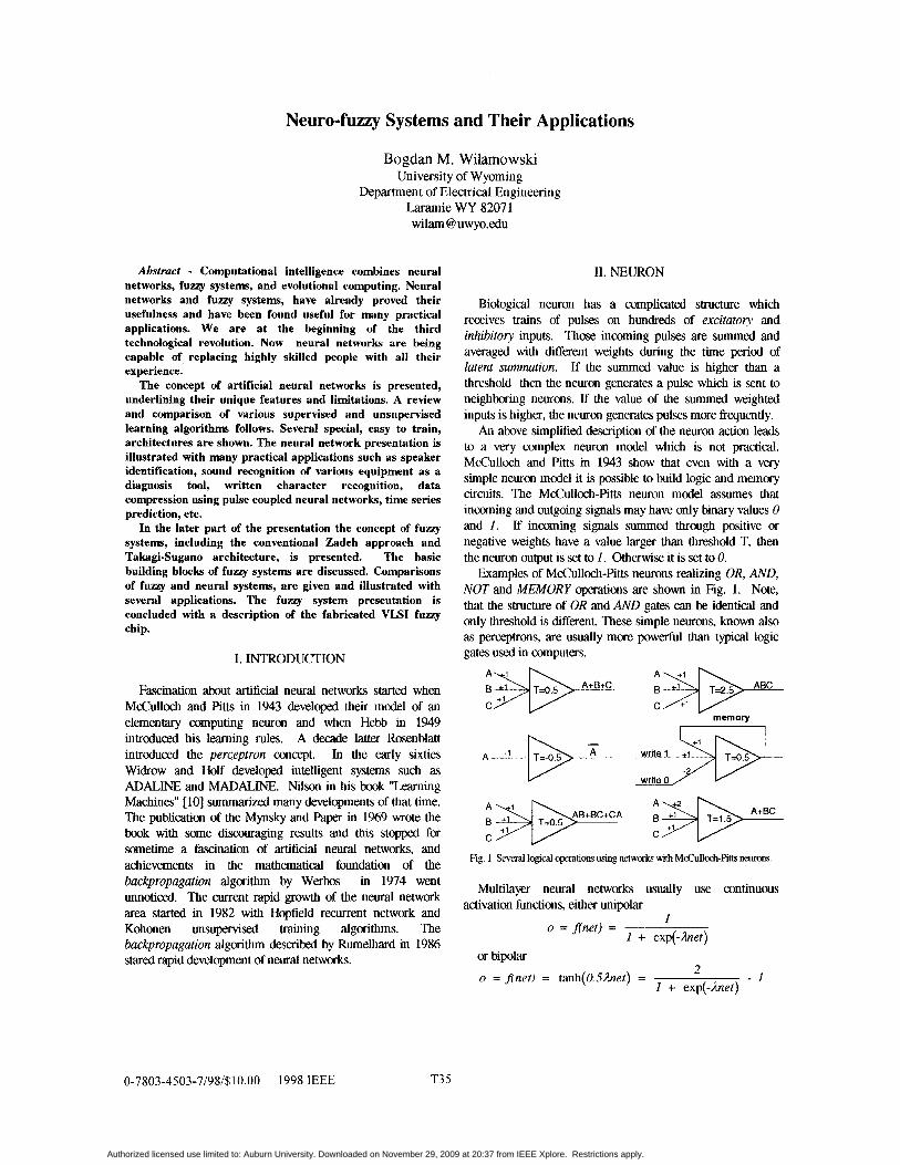
Biological neuron has a complicated structure which receives trains of pulses on hundreds of excitatory and inhibitory inputs. Those incoming pulses are summed and averaged with different weights during the time period of latent sumnution. If the summed value is higher than a threshold then the neuron generates a pulse which is sent to neighboring neurons. If the value of the summed weighted inputs is higher, the neuron generates pulses more iiequently.

An above simplified description of the neuron action leads to a very complex neuron model which is not practical. McCulloch and Pitts in 1943 show that even with a very simple neuron model it is possible to build logic and memory circuits. The McCulloch-Rtts neuron model assumes that incoming and outgoing signals may have only binary values 0 and 1. If incoming signals summed through positive or negative weights have a value larger than threshold T, then the neuron output is set to 1. Otherwise it is set to 0.

Examples of McCulloch-Pitts neurons realizing OR, AND, NOT and MEMORY operations are shown in Fig. 1. Note, that the structure of OR and AND gates can be identical and only threshold is different. These simple neurons, known also as perceptrons, are usually more powerful than typical logic gam used in computers.

memory - A *' write 1

write 0

A+BC

Fig. 1 Several lcgical opentiom using netwcrks with McCulla;h-pitts neurons.

Multilayer neural networks usually use continuous activation functions, either unipolar

I 1 + exp(-het)

o = ffnet) =

or bipolar o = j n e t ) = tanh(0.5het) = - 1

2 I + exp(-het)

0-7803-4503-7198/$10.00 1998 IEEE T3 5

Authorized licensed use limited to: Auburn University. Downloaded on November 29, 2009 at 20:37 from IEEE Xplore. Restrictions apply.

mailto:[email protected]

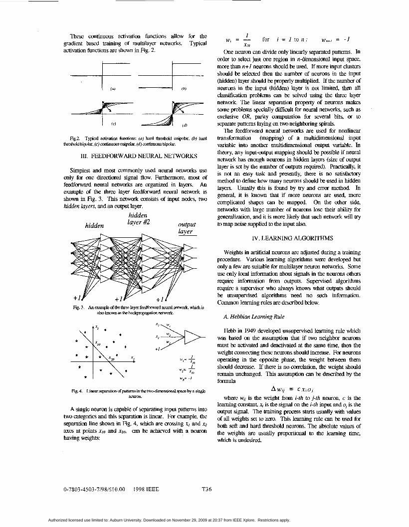
These continuous activation functions allow for the Typical gradient based training of multilayer networks.

activation functions are shown in Fig. 2.

+ + ---

Fig.2. Typical adivation funciions: (a) hard threshdd unipolar. (b) hard b h l d bipolar, (c) Continuous unipolar, (d) continucus bipdar.

111. W-EDFORWARD NEURAL NETWORKS

Simplest and most commonly used neural networks use only for one directional signal flow. Furthermore, most of feedforwad neural networks are organized in layers. An example of the three layer feedforward neural network is shown in Fig. 3. This network consists of input nodes, two hidden layers, and an output layer.

hidden hidden layer #2 output

h layer h

Fig. 3. An exanple ofthe three layer feedfonvard neural network, which is also known as the backprcpgation network

w3= - I

Fig. 4. Linear separation ofpaaerns in the two-dimensional space by a single neuron.

A single neuron is capable of separating input patterns into two categories and this separation is linear. For example, the separation line shown in Fig. 4, which are crossing xl and x2 axes at points xlo and xzo, can be achieved with a neuron having weights:

0-7803-4503-7/98/$10.00 1998 IEEE T3 6

for i = 1 to n : w,,+~ = - 1 I M.', = -

x,o One neuron can divide only linearly separated patterns. In

order to select just one region in n-dimensional input space, more than n+l neurons should be used. If more input clusters should be selected then the number of neurons in the input (hidden) layer should be properly multiplied. If the number of neurons in the input (hidden) layer is not limited, then all classification problems can be solved using the three layer network. The linear separation property of neurons makes some problems spectally difficult for neural networks, such as exclusive OR, parity computation for several bits, or to separate patterns laying on two neighboring spirals.

The feedfaward neural networks are used for nonlinear transformation (mapping) of a multidimensional input variable into another multidimensional output variable. In theory, any input-output mapping should be possible if neural network has enough neurons in hidden layers (size of output layer is set by the number of outputs required). Practically, it is not an easy task and presently, there is no satisfactory method to define how many neurons should be used in hidden layers. Usually this is found by try and error method. In general, it is known that if more neurons are used, more complicated shapes can be mapped. On the other side, networks with large number of neurons lose their ability for generalization, and it is more likely that such network will try to map noise supplied to the input also.

IV. LEARNING ALGORITHMS

Weights in artificial neurons are adjusted during a training procedure. Various learning algorithms were developed but only a few are suitable for multilayer neuron networks. Some use only local information about signals in the neurons others require information Erom outputs. Supervised algorithms require a supervisor who always knows what outputs should be unsupervised algorithms need no such information. Common learning rules are described below.

A. Hebbian Learning Rule

Hebb in 1949 developed unsupervised learning rule which was based on the assumption that if two neighbor neurons must be activated and deactivated at the same time, then the weight connecting these neurons should increase. For neurons operating in the opposite phase, the weight between them should decrease. If there is no melation, the weight should remain unchanged. This assumption can be described by the formula

Awij = cxioj where wij is the weight !Yom i-th toj-th neuron, c is the

learning constant, Xi is the signal on the i-th input and oj is the output signal. The training process starts usually with values of all weights set to zero. This learning rule can be used for both soft and hard threshold neurons. The absolute values of the weights are usually proportional to the learning time, which is undesired.


B. Correlation leoming rule

The correlation lewning rule uses a similar principle as the Hebbian learning rule. It assumes that weights between simultaneously respcklding neurons should be largely positive, and weights between neurons with opposite reaction should be largely negative. hriathematically, this can be written that weights should be proportional to the product of states of connected neurons. In contrary to the Hebbian rule, the melation rule is of the supervised type. Instead of actual response, the desired response is used for weight change calculation

A W , = C X I ~ J

This training algcirithm starts with initialization of weights to zero values.

C. Instar leaminlt rule

If input vectors, and weights, are normalized, or they have only binary bipolar values (-I or +Z), then the net value will have the largest pabitive value when the weights have the same values as the iniput signals. Therefore, weights should be changed only if they pre different from the signals

A w , = C ( X , - w, ) Note, that the infbrmation required for the weight is only

taken kom the input signals. This is a local and unsupervised learning algorithm.

D. W A - Winner Takes All The WTA is a madifioltion of the instar algorithm where

weights are modifiedl only for the neuron with the highest net value. Weights of remaining neurons are left unchanged. This unsupervised algorithm @"e we do not know what are desired outputs) has a global character. The WTA algorithm, developed by Kohonien in 1982, is often used for autmatic clustering and for extracting statistical properties of input data.

E. Outstar leamiizg rule

In the outstar leaning rule it is required that weights connected to the cerlain node should be equal to the desired outputs for the neurons connected through those weights

A w , = C ( d j - wij)

where 4 is the desired neuron output and c is small learning constant which mer decreases during the learning procedure. This is the supervised training procedure because desired outputs must be known. Both instar and outstar learning rules were developed by Grossberg in 1974.

F. Widrow-Hoff (LMS) learning nile

Widrow and Hoff in 1962 developed a supervised training algorithm which allows to train a neuron for the desired response. This rule was derived by minimizing the square of the difference between ner and output value.

0-7803-4503-7/98/$10.00 1998 IEEE T3 7

p = l

where Error, is the error forj-th neuron, P is the number of applied patterns, db is the desired output forj-th neuron when p-th pattern is applied. This rule is also known as the LMS (Least Mean Square) rule. By calculating a derivative of the error with respect to wi, one can find a formula for the weight change.

p = l

Note, that weight change Awij is a sum of the changes from each of the individual applied patterns. Therefore, it is possible to correct weight after each individual pattern was applied. If the learning constant c is chosen to be small, then both methods gives the same result. The LMS rule works well for all type of activation functions. This rule tries to enforce the net value to be equal to desired value. Sometimes, this is not what we are looking for. It is usually not important what the net value is, but it is important if the net value is positive or negative. For example, a very large net value with a proper sign will result in large error and this may be the preferred solution.

G. Linear regression

The LMS learning rule requires hundreds or thousands of iterations before it converges to the proper solution. Using the linear regression the same result can be obtained in only one step.

Considering one neuron and using vector notation for a set of the input patterns X applied through weights w the vector of net values net is calculated using

Xw = net where X is a rectangular array (n+I)*p, n is the number of

inputs, and p is the number of patterns. Note that the size of the input patterns is always augmented by one, and this additional weight is responsible for the threshold. This method, similar to the LMS rule, assumes a linear activation function, so the net values net should be equal to desired output values d

xw = d Usuallyp > n+Z, and the above equation can be solved only

in the least mean square error sense w =(XTX)'XTd

or to convert the set of p equations with n+l unknowns to the set of n+Z equations with n+I unknowns. Weights are a solution of the equation

Yw = 2

where elements of the Y matrix and the z vector are given by

P P

p = l p d


H. Delta learning rule

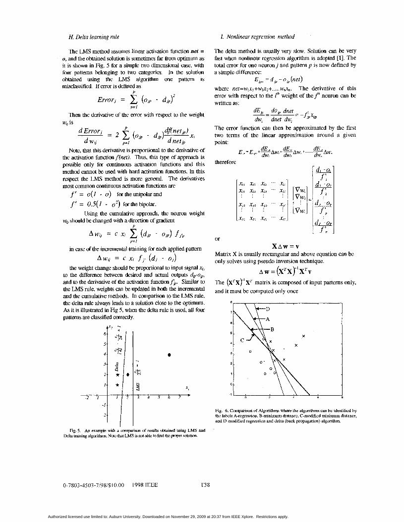
The LMS method assumes linear activation function net = 0, and the obtained solution is sometimes far from optimum as it is shown in Fig. 5 for a simple two dimensional case, with four pattems belonging to two categories. In the solution obtained using the LMS algorithm one pattern is misclassified. If error is defined as

D

Errorj = 2 ( o j p - djp)l p= I

Then the derivative of the error with respect to the weight U:.; is

Note, that this derivative is proportional to the derivative of the activation function f(net). Thus, this type of approach is possible only for continuous activation functions and this method Canna be used with hard activation functions. In this respect the LMS method is more general. The derivatives most common continuous activation functions are

f' = o(l - 0) for the unipolar and f' = 0.5(1 - 02) forthebipolar.

Using the cumulative approach, the neuron weight M ' ~ ~ should be changed with a direction of gradient

P

p = l

in case of the incremental training for each applied pattern

the weight change should be proportional to input signal x,, to the difkrence between desired and actual outputs dp-op, and to the derivative of the activation function 7,. Similar to the LMS rule, weights can be updated in both the incremental and the cumulative methods. In comparison to the LMS rule, the delta rule always leads to a solution close to the optimum. As it is illustrated in Fig 5, when the delta rule is used, all four patterns are classified correctly.

AWIJ - - c XI fJ, (d, - 0,)

I. Nonlinear regression method

'I'he delta method is usually very slow. Solution can be very fast when nonlinear regression algorithm is adopted [l]. The total error for one neuron j and pattern p is now defined by a simple difference:

where net=w1x1+w2x2+ ..... wnxn. The derivative of this error with respect to the ifh weight of the j" neuron can be written as:

= d J p - o J p ( r l e t )

dEJp - do, dnet -_--- d y dnet d y - -f,x,,

The error function can then be approximated by the first two terms of the linear approximation around a given mint:

therefore

I""]- vw,

or X A w = v

Matrix X is usually rectangular and above equation can be only solves using pseudo inversion technique.

A w = (X'X)-* XTv The (X7X)'XT matrix is composed of input pattems only, and it must be computed only once

8 I

Fig. 6. Comparison of Algorithm where the algorithms can be identified by the labels A-regression, B-nunimum distance. C-modified nunimum distance. and D-modified regression and delta (back propagation) algonthm.

Rp. 5. An example with a comparison of results obtained using LMS and Delta training a l g a i h . Note that LMS is not able to find the proper solution.

0-7803-4503-7/98/$10.00 1998 IEEE T3 8


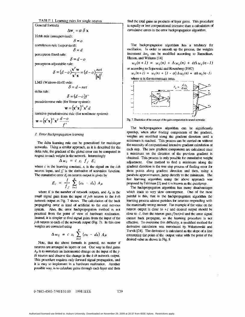
TABLE 1. Learning rules for single neuron General formula

Hebb rule (unsupeirvised):

correlation rule (supervised):

perceptron fixed rale:

perceptron adjustable rule:

Awl = a S x

6=0

S = d

6 Z d - o

XTW net 6 = (d -0)- = (d - o ) ~ llX11

xTx LMS (Widrow-Hoff) rule:

delta rule:

pseudoinverse rule (for linear system):

w = (x'x)-'x'd iterative pseudoinverse rule (for nonlinear system):

6 = d -net

6 = (d - 0 ) f '

T d -0 w = (x'x)'x -- f '

J. Error Backpropagation leaming

The delta learning rule can be generalized for multilayer networks. Using a :similar approach, as it is described for the delta rule, the gradient of the global error can be computed in respect to each weight in the network. Interestingly

where c is the learning constant, x, is the signal on the i-th neuron input, and j;' is the derivative of activation function. The cumulative error E, on neuron output is given by

A WIJ = c X I f J l E,

J J' k=I

where K is the number of network outputs, and Alk is the small signal gain fjrom the input of j-th neuron to the k-th network output as Fig. 7 shows. The calculation of the back propagating error is kind of artificial to the real nervous system. Also, the error backpropagation method is not practical from the point of view of hardware realization. Instead, it is simpler to find signal gains firom the input of the j-th neuron to each of the network output (Fig. 7). In this case weights are corrected using

K

k=1 Note, that the above formula is general, no matter if

neurons are arranged in layers or not. One way to find gains A$ is to introduce ani incremental change on the input of the j - th neuron and observe the change in the k-th network output. This procedure requires only forward signal propagation, and it is easy to implenrent in a hardware realization. Another pcxsible way, is to calculate gains through each layer and then

0-7803-4503-7/98/5:10.00 1998 IEEE T3 9

find the total gains as products of layer gains. This procedure is equally or less computational intensive than a calculation of cumulative errors in the error backpropagation algorithm.

The backpropagation algorithm has a tendency for oscillation. In order to smooth up the process, the weights increment Aw,, can be modified acccording to Rumelhart, Hinton, and Wiliams [ 141

or according to Sejnowski and Rosenberg (1987) W l J ( n + I ) = w l J ( n ) + AWIJ(n) + a W t J ( n - l )

w,(n + 1) = wg (n) + (1 - a) A w,, (n) + U!, w,, (n - 1 ) where a is the momentum term. r-------- 1

i

+ I Y Fig. 7. illustration dthe c o n q ofthe gain computation in neural networks

The backpropagation algorithm can be significantly speedup, when after finding components of the gradient, weights are modified along the gradient direction until a minimum is reached. This process can be carried on without the necessity of computational intensive gradient calculation at each step. The new gradient components are calculated once a minimum on the direction of the previous gradient is obtained. This process is only possible for cumulative weight adjustment. One method to find a minimum along the gradient direction is the tree step process of finding error for three points along gradient direction and then, using a parabola approximation, jump direcxly to the minimum. The fast learning algorithm using the above approach was proposed by Fahlman [2] and it is known as the quickprop.

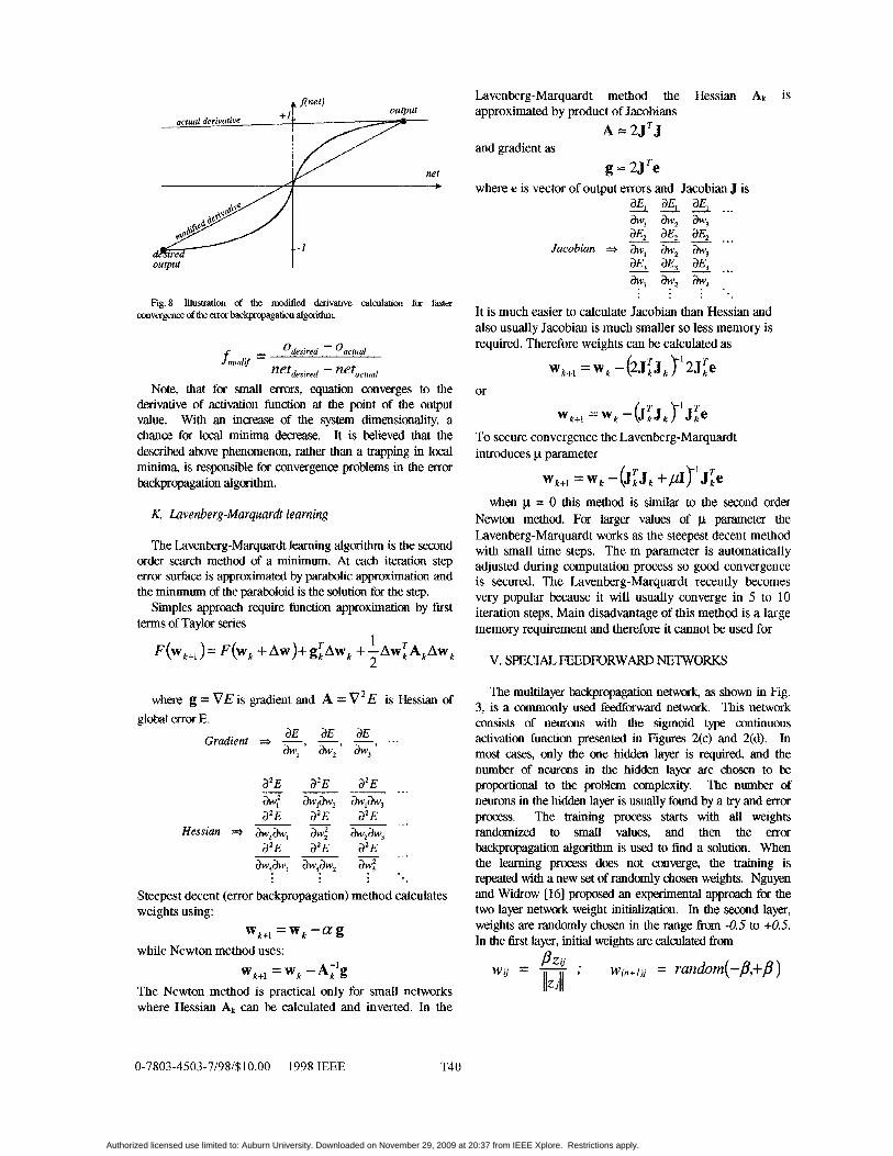
The backpropagation algorithm has many disadvantages which leads to very slow convergence. One of the most painful is this, that in the backpropagation algorithm the learning process almost perishes for neurons responding with the maximally wrong answer. For example if the value on the neuron output is close to + I and desired output should be close to - I , then the neuron gainf(nett-0 and the error signal cannot back propagate, so the learning procedure is not effective. To overcome this difficulty, a modified method for derivative calculation was introduced by Wilamowski and Torvik [a]. The derivative is calculated as tQe slope of a line connecting the point of the output value with the point of the desired value as shown in Fig. 8


output I

Wg.8 IllustratiOn of the modified derivative calmlation fa fa= mvergence ofthe enor baclqropagation algorithm

- Odesired - oacmal

netdesired - netactual

Note, that for small errors, equation converges to the derivative of activation function at the point of the output value. With an increase of the system dimensionality, a chance for local minima decrease. It is believed that the described above phenomenon, rather than a trapping in local minima, is responsible for convergence problems in the error backpropagation algorithm.

K. Lavenberg-Marquardt learning

The Lavenberg-Marquardt learning algorithm is the second order search method of a minimum. At each iteration step error surface is approximated by parabolic approximation and the minimum of the paraboloid is the solution for the step.

Simples approach require function approximation by first terms of Taylor series

1 2

F ( w ~ + ~ ) = F(wk +Aw)+g:Aw, i--Aw:AkAwk

where g = V E is gradient and A = V 2 E is Hessian of global error E.

dE aE aE Gradient -, - - ... my, a W 2 * aw,'

a 2 E a 2 E a 2 E

a 2 E a 2 E a Z E

a 2 E a'E d 2 E

- - - ... w &,my, - - ~ ...

Hessian * aw2aw, &*;z &&J3

- - - ... a W 3 . a w l "v, my: .

Steepest decent (error backpropagation) method calculates weights using:

while Newton method uses: Wk+l = wk -a g

Wk+l = wk -A,'g The Newton method is practical only for small networks where Hessian Ak can be calculated and inverted. In the

Lavenberg-Marquardt method the Hessian AI, is approximated by product of Jacobians

A = 2JTJ and gradient as

where e is vector of output errors and Jacobian J is g = 2JTe

- - aE, aE, aE, .-. my, my, my,

- - aE, aE, aE, ... e* hyz hu" .

aEZ aE2 aE, Jacobian * my, &J2 &J3

- - - ...

.~

It is much easier to calculate Jacobian than Hessian and also usually Jacobian is much smaller so less memory is required. Therefore weights can be calculated as

or

Wk+l = wk - (J:J, I'JEe To secure convergence the Lavenberg-Marquardt introduces p parameter

when p = 0 this method is similar to the second order Newton method. For larger values of p parameter the Lavenberg-Marquardt works as the steepest decent method with small time steps. The m parameter is automatically adjusted during computation process so good convergence is secured. The Lavenberg-Marquardt recently becomes very popular because it will usually converge in 5 to 10 iteration steps. Main disadvantage of this method is a large memory requirement and therefore it cannot be used for

V. SPECIAL FEEDFORWARD NETWORKS

The multilayer backpropagation network, as shown in Fig. 3, is a commonly used feedforwad network. This network consists of neurons with the sigmoid type continuous activation function presented in Figures 2(c) and 2(d). In most cases, only the one hidden layer is required, and the number of neurons in the hidden layer are chosen to be propartional to the problem complexity. The number of neurons in the hidden layer is usually found by a try and error process. The training process starts with all weights randomized to small values, and then the error backpropagation algorithm is used to find a solution. When the leaming process does not converge, the training is repeated with a new set of randomly chosen weights. Nguyen and Widrow [16] proposed an experimental approach for the two layer network weight initialization. In the second layer, weights are randomly chosen in the range fiom -0.5 to +0.5. In the first layer, initial weights are calculated from

0-7803-4503-7/98/$10.00 1998 IEEE T40


where 5, is the mdom number firom -0.5 to +0.5 and the

p = 0 . 7 P ~ where n is the number of inputs, and N is the number of

hidden neurons in the first layer. This type of weight initialization usually leads to faster solutions.

For adequate solutions with backpropagation networks, many tries are typically required with different network structures and different initial random weights. This encouraged researchers to develop feedforward networks which can be more reliable. Some of those networks are described below.

scaling factor i3 is given by I

A. Functional lit& nenvork

One layer neural networks are relatively easy to train, but these networks can solve only linearly separated problems. The concept of furictional link networks was developed by Nilson bodc [lo] and late elaborated by Pa0 [13] using the functional link network shown in Fig. 9.

0

.... 4

0 &

U Fig. 9. The fundional link netwcrk

Using nonlinear terms with initially determined functions, the actual number of inputs supplied to the one layer neural network is increasecl. In the simplest case nonlinear elements are higher order tcms of input patterns. Note that the functional link network can be treated as a one layer network, where additional input data are generated off line using nonlinear transformations. The learning procedure for one layer is easy and fast. Fig. 10 shows an XOR problem solved using functional link networks. Note, that when the functional link approach is used, this difficult problem becomes a trivial one. The problem with the functional link network is that p r o p selection of nonlinear elements is not an easy task. However, in many practical cases it is not difficult to predict what kind of transformation of input data may linearize the problem, so the functional link approach can be used.

untpolcrr neuron bipolar neuron

Fig. 10 Funtional link networks for sdution ofthe XOR problem: (a) using unipdar signals, (b) using bipolar signals.

0-7803-4503-7/98/$10.00 1998 IEEE T4 1

Kohonen Grossberg layer I'\ o layer

summing unipolar circuits neurons

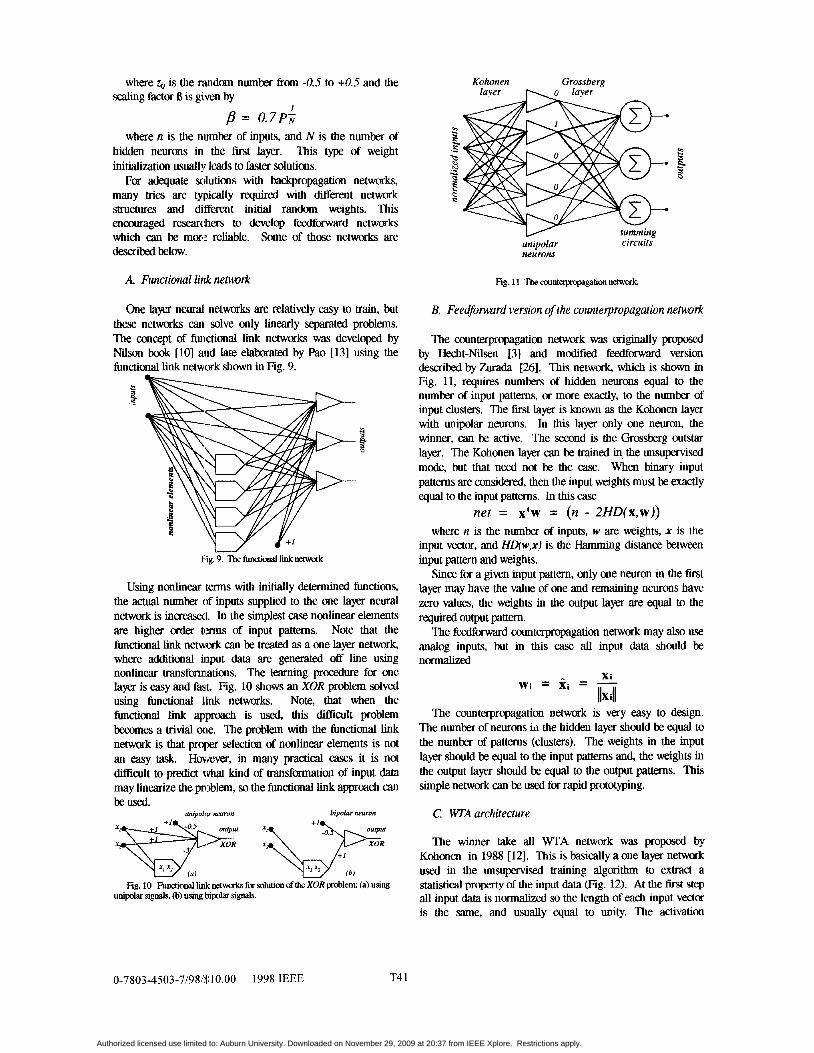
Fig. 11 The ccunterpropagaton network.

B. Feedforward version of the counterpropagation network

The counterpropagation network was originally proposed by Hecht-Nilsen [3] and modified feedfbrward version described by &ada [26]. This network, which is shown in Fig. 11, requires numbers of hidden neurons equal to the number of input patterns, or more exactly, to the number of input clusters. The first layer is known as the Kohonen layer with unipolar neurons. In this layer only one neuron, the winner, can be active. The second is the Grossberg outstar layer. The Kohonen layer can be trained in the unsupervised mode, but that need not be the case. When binary input patterns are considered, then the input weights must be exactly equal to the input patterns. In this case

net = x'w = (n - 2HD(x,w)) where n is the number of inputs, w are weights, x is the

input vector, and HD(w,x) is the Hamming distance between input pattern and weights.

Since for a given input pattern, only one neuron in the first layer may have the value of one and remaining neurons have zero values, the weights in the output layer are equal to the required output pattern.

The feedforward counterpropagation network may also use analog inputs, but in this case all input data should be normalized

A Xi = - w i = x i llXi l l

The counterpropagation network is very easy to design. The number of neurons i ~ i the hidden layer should be equal to the number of patterns (clusters). The weights in the input layer should be equal to the input patterns and, the weights in the output layer should be equal to the output patterns. This simple network can be used for rapid prototyping.

C. WA architecture

The winner take all WTA network was proposed by Kohonen in 1988 [12]. This is basically a one layer network used in the unsupervised training algorithm to extract a statistical property of the input data (Fig. 12). At the first step all input data is normalized so the length of each input vector is the same, and usually equal to unity. The activation


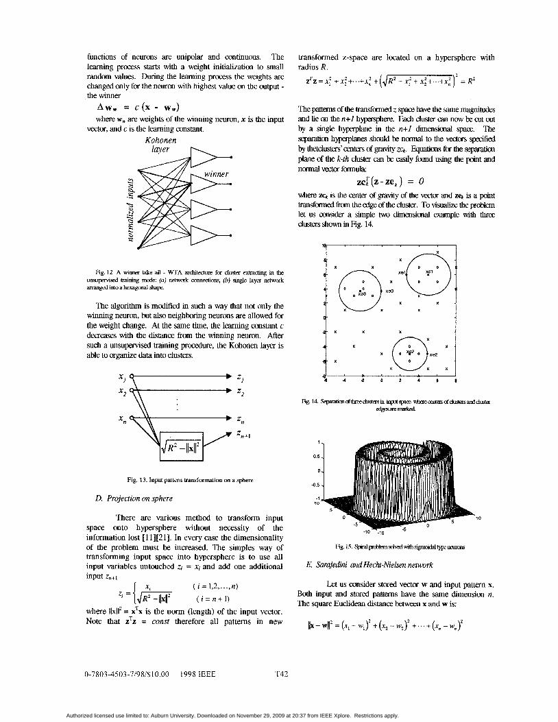
functions of neurons are unipolar and continuous. The learning process starts with a weight initialization to small random values. During the learning process the weights are changed only for the neuron with highest value on the output - the winner

Aww = c ( x - ww) where w, are weights of the winning neuron, x is the input

vector, and c is the learning constant. Kohonen

2 Y

-a 2 2

s tu‘ -a Y

r? 0 s2

Fig. 12 A winner take all - “TA architemre for cluster extrading in the unsupwvised training mode: (a) network COM&O~S, (b) single layer network arranged into a hexagonal +.

The algorithm is modified in such a way that not only the winning neuron, but also neighboring neurons are allowed for the weight change. At the same time, the learning constant c decreases with the distance Erom the winning neuron. After such a unsupervised training procedure, the Kohonen layer is able to organize data into clusters.

Fig. 13. Input pattern transformation on a sphere

D. Projection on sphere

There are various method to transform input space onto hypersphere without necessity of the information lost [11][21]. In every case the dimensionality of the problem must be increased. The simples way of transforming input space into hypersphere is to use all input variables untouched zi = xi and add one additional input z “ + ~

( i = 1,2, ..., n) zl ={4* ( i = n + l )

where llxll’ = xTx is the norm (length) of the input vector. Note that zTz = const therefore all patterns in new

transformed z-space are located on a hypersphere with radius R .

z T z = x ~ +x:+...+xi +(, /Rz -x: +x:+...+x~)* = R2

The p a m s of the transfmed z space have the same magnitudes and lie on the n+l hypesphere. Fach cluster can now be cut out by a single hyperplane in the n+l dimensional space. Ihe separaticpl hypsplanes should be normal to the vectars speakcl

plane of the k-th cluster can be easily found using the point and normal vector formula:

by thet~l~~tfXS’ CentfXS of @Ivity ZCk. ~ U C l h S fOr the S€pX2lbtl

zcl(z-ze,) = o where z c k is the center of gravity of the vector and q is a point transfmed &om the edge of the cluster. To visualize the problem let us consider a simple two dimensional example with three clusters shown in Fig. 14.

E Sarajedini and Hecht-Nielsen network

Let us consider stored vector w and input pattern x. Both input and stored patterns have the same dimension n. The square Euclidean distance between x and w is:

0-7803-4503-7/98/$10.00 1998 IEEE T42


After defactorizatioti

finally

where net = xTw is the weighted sum of input signals. Fig. 16 shows the netRork which is capable of calculating the square of Euclidean distance between input vector x and stored pattern w.

i t x - ~ ' =.r; + x i + . . . + X i +%$ +w,'+...+Wn'-2(x1w; +X21+\ +...+ X"1V")

Ik - wllZ = x T x + wTw - 2xTw = 11x112 + 1 1 ~ 1 1 2 - 2net

500

400

300

200

100

0 30

30

0-0

Fig. 16. Network capable of calculating square of Euclidean distance between input pattemx ;md stored pattern w. (a) network; (b) Euclidean distance calculation forrn vector (15,15)

In order to calculate the square of Euclidean distance the following mod] fications are required: (i) bias equal to Ilwll', (ii) additional input with square of input vector magnitude llwIl2, and (iii) weights equal to components of stored vector multiplied by -2 factor. Note that when additional input with the square of magnitude is added than simple weighted sum type of network is capable of calculating square of Euclidean distance between x and w. This approach can be directly incorporated into RBF and LVQ networks.

With the approach presented on Fig. 2 several neural network techniques such as RBF, LVQ, and GR can be used with classical weighted sum type neurons without necessity of computing the Euclidean distance in a traditional way. All what is required is to add additional input with the magnitude of the input pattem.

E. Cascade corrdarion architecture

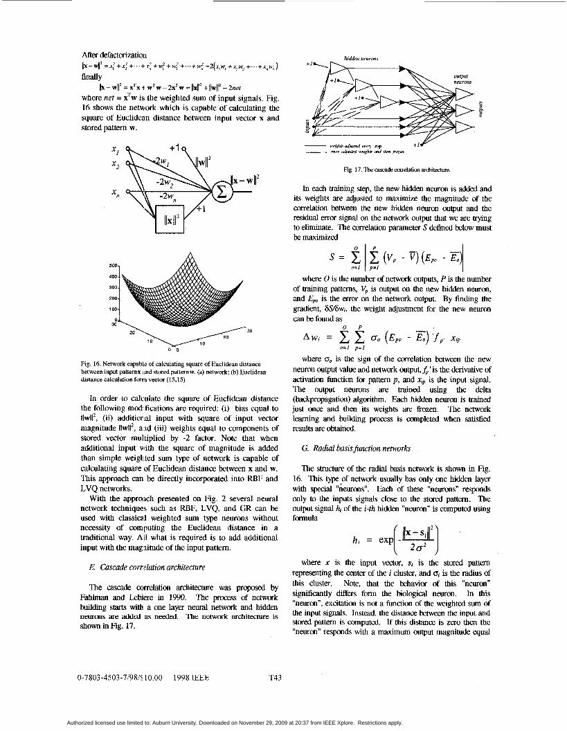
The cascade coirrelation architecture was proposed by Fahlman and Lebiere in 1990. The process of network building starts with a one layer neural network and hidden neurons are added as needed. The network architecture is shown in Fig. 17.

0-7803-4503-7/981$10.00 1998 IEEE T43

hidden neurons

Fig. 17. The cascade carelation architeuure.

In each training step, the new hidden neuron is added and its weights are adjusted to maximize the magnitude of the correlation between the new hidden neuron output and the residual error signal on the network output that we are trying to eliminate. The correlation parameter S defined below must be maximized

- s = 1 (v, - v) ( E , - E)J

o=I ,=I

where 0 is the number of network outputs, P is the number of training patterns, V, is output on the new hidden neuron, and E,, is the error on the network output. By finding the gradient, ~SW;,, the weight adjustment for the new neuron can be found as

O P

o=l p = l

where 0, is the sign of the correlation between the new neuron output value and network output, &, ' is the derivative of activation function for pattern p, and xt, is the input signal. The output neurons are trained using the delta (backpropagation) algorithm. Each hidden neuron is trained just once and then its weights are fkozen. The nehork learning and building process is completed when satisfied results are obtained.

G. Radial basisfunction networks

The structure of the radial basis network is shown in Fig. 16. This type of network usually has only one hidden layer with special "neurons". Each of these "neurons" responds only to the inputs signals close to the stored pattem. The output signal h, of the i-th hidden "neuron" is computed using formula

hi = exp ( -- llx;--;lr] where x is the input vector, s, is the stored pattern

representing the center of the i cluster, and q is the radius of this cluster. Note, that the behavior of this "neuron" significantly differs form the biological neuron. In this "neuron", excitation is not a function of the weighted sum of the input signals. Instead, the distance between the input and stored pattern is computed. If this distance is zero then the "neuron" responds with a maximum output magnitude equal


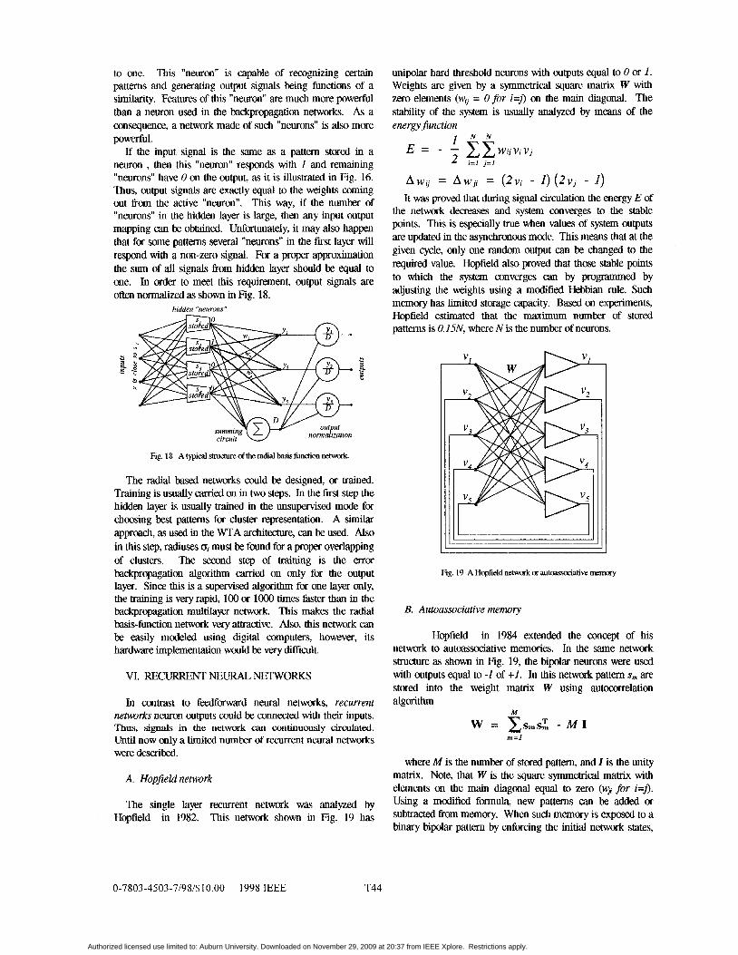
to one. This "neuron" is capable of recognizing certain patterns and generating output signals being functions of a similarity. Features of this "neuron" are much more powerful than a neuron used in the bckpropagation networks. As a consequence, a network made of such "neurons" is also more powerful.

If the input signal is the same as a pattern stored in a neuron , then this "neuron" responds with 1 and remaining "neurons" have 0 on the output, as it is illustrated in Fig. 16. Thus, output signals are exactly equal to the weights coming out from the active "neuron". This way, if the number of "neurons" in the hidden layer is large, then any input output mapping can be obtained. Unfortunately, it may also happen that for some pattems several "neurons" in the first layer will respond with a non-zero signal. For a proper approximation the sum of all signals from hidden layer should be equal to one. In order to meet this requirement, output signals are often normalized as shown in Fig. 18.

hidden "neurons"

Fig. 18 A typical structure ofthe radial basis fundion network.

The radial based networks could be designed, or trained. Training is usually carried on in two steps. In the first step the hidden layer is usually trained in the unsupenised mode for choosing best pattems for cluster representation. A similar approach, as used in the WTA architecture, can be used. Also in this step, radiuses must be found for a proper overlapping of clusters. The second step of training is the error backpropagation algorithm carried on only for the output layer. Since this is a supervised algorithm for one layer only, the training is very rapid, 100 or lo00 times faster than in the backpropagation multilayer network. This makes the radial basis-function network very attractive. Also, this network can be easily modeled using digital computers, however, its hardware implementation would be very difficult.

VI. RECURRENT NEURAL NETWORKS

In contrast to feedforward neural networks, recurrent networks neuron outputs could be connected with their inputs. Thus, signals in the network can continuously circulated. Until now only a limited number of recurrent neural networks were described.

A. Hopfield network

The single layer recurrent network was analyzed by Hopfield in 1982. This network shown in Fig. 19 has

unipolar hard tlireshold neurons with outputs equal to 0 or 1. Weights are given by a symmetrical square matrix W with zero elements (N;, = 0 for i=j) on the main diagonal. The stability of the system is usually analyzed by means of the energy function

I N N E = - - ~ J ~ d w , v l v j

2 1=1 j=1

Aw,] = Awjl = (2v, - I) (2v, - I ) It was proved that during signal circulation the energy E of

the network decreases and system converges to the stable points. This is especially true when values of system outputs are updated in the asynchronous mode. This means that at the given cycle, only one random output can be changed to the required value. Hopfield also proved that those stable points to which the system converges can by programmed by adjusting the weights using a modified Hebbian rule. Such memory has limited storage capacity. Based on experiments, Hopfield estimated that the maximum number of stored patterns is 0.1 SN, where N is the number of neurons.

Fig. 19 A Hopfield network OT au"ciat ive mmry

B. Autoassociative memory

Hopfield in 1984 extended the concept of his network to autoassociative memories. In the same network structure as shown in Fig. 19, the bipolar neurons were used with outputs equal to -1 of + I , In this network pattern s,,, are stored into the weight matrix W using autmelation algorithm

M w = &sT, - M I

m = l

where M is the number of stored pattern, and Z is the unity matrix. Note, that W is the square symmetrical matrix with elements on the main diagonal equal to zero (wj for i=j). Using a modified formula, new patierns can be added or subtracted from memory. When such memory is exposed to a binary bipolar pattern by enforcing the initial network states,

0-7803-4503-7198/$10.00 1998 IEEE T44


then after signal circulation the network will converge to the closest (most similar) stored pattern or to its complement. This stable point will be at

I 2

E(v) = - -vTWv

the closest minimum of the energy functionLike the Hopfield network, the autoassociative memory has limited storage capacity, which is estimated to be about Mm=0.15N. When the number of stored patterns is large and close to the memory capacity, the network has a tendency to converge to spurious states which were not stored. These spurious states are additional minima of the energy function.

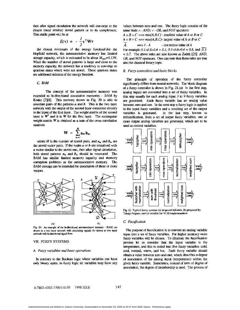
C. BAM

The concxpt of the autoaSSoCiative memory was extended to bidirectional associative memories - BAM by Kosko [7][8]. This memory shown in Fig. 20 is able to associate pairs of the patterns a and b. This is the two layer nmork with the output of the second layer connected directly to the input of the first layer. The weight matrix of the second layer is WT and it is W for the first layer. The rectangular weight matrix W is obtained as a sum of the cross melation matrixes

M W = Camb,

m=l

where M is the number of stored pairs, and U,,, and 6, are the stored vector pairs. If the nodes a or b are initialized with a vector similar to the stored one, then after signal circulation, both stored patterns U,,, and b, should be recovered. The BAM has similar limited memory capacity and memory corruption problem!; as the autoassociative memory. The BAM concept can Ix: extended for association of three or more vectors.

(4 (b) Fig. 20. An example of the bid ired id autoasudive nlemuy - BAh4: (a) drawn as a two layer net\& with cira~lating signals (b) drawn as two layer network with bi-diredional signal flow.

VII. FUZZY SYS’IEMS

A. Fuzzy variables and basic operations

In contrary to the Boolean logic where variables can have only binary states, ixi fuzzy logic all variables may have any

0-7803-4503-7/98/!i10.00 1998 IEEE T45

values W e e n zero and one. The fuzzy logic consists of the same basic A - AND, v - OR, and NOT operators: A A B A C ==> min(A, B. C] - smallest value of A or B or C A v B v C ==> m ( A , B, C)- largest value of A or B or C A = > I - A - one minus value of A Forexample0.1~0.8~0.4 = O.l,O.IvO.8v0.4 = 0.8, and 0.3 = 0.7. The above rules are also known as Zadeh [25] AND, OR, and NOT operators. One can note that these rules are true also for classical binary logic.

-

B. Fuzzy controllers and basic blocks

The principle of operation of the fuzzy controller significantly differs kom neural networks. The block diagram of a fuzzy controller is shown in Fig. 21.(a) In the first step, analog inputs are converted into a set of fuzzy variables. In this step usually for each analog input 3 to 9 fuzzy variables are generated. Each fuzzy variable has an analog value between zero and one. In the next step a fuzzy logic is applied to the input fuzzy variables and a resulting set of the output variables is generated. In the last step, known as defuzzification, firom a set of output fuzzy variables, one or more output analog variables are generated, which are to be used as control variables.

U 7

I

Fig. 21. Typical fuzzy systems (a) proposed b-deh, @) proposed by Takagi-Sugano, and (c) suitable for VLSI implementation

C. Fum>cation

The purpose of fuzzification is to convert an analog variable input into a set of fuzzy variables, For higher accuracy more fuzzy variables will be chosen. To illustrate the fuzzification process let us consider that the input variable is the temperature, and this is coded into five fuzzy variables: cold, cool, normal, warm, and hot. Each fuzzy variable should obtain a value between zero and one, which describes a degree of association of the analog input (temperature) within the given fuzzy variable. Sometimes, instead of term of degree of association, the degree of membership is used. The process of


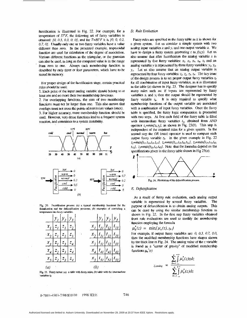
fuzzification is illustrated in Fig. 22. For example, for a temperature of V F , the following set of fuzzy variables is obtained: [O, 0.5, 0.3, 0, 01, and for T=80"F it is [O, 0, 0.2, 0.7, 01. Usually only one or two fuzzy variables have a value diffsent than zero. In the presented example, trapezoidal function are used for calculation of the degree of association. Various different functions as the triangular, or the gaussian can also be used, as long as the computed value is in the range from zero to one. Always each membership function is described by only three or four parameters, which have to be stored in memory.

Yl y 2

' 1 '11 t12

' 2 t21 '22

' 3 t31 32 t t

' 4 '41 t42

' 5 '51 t t 52

For proper design of the fuzzification stage, certain practical rules should be used: 1. Each point of the input analog variable should belong to at least one and no more then two membership functions. 2. For overlapping functions, the sum of two membership functions must not be larger than one. This also means that overlaps must not cross the points of maximum values (ones). 3. For higher accuracy, more membership function should be used. However, very dense functions lead to a frequent system reaction, and sometimes to a system instability.

574 8 0 4 cold

shown in Fig. 22. In the first step fuzzy variables obtained from rule evaluations are used to modify the membership function employing the f m u l a

For example, if output fuzzy variables are: 0, 0.3, 0.7, 0.0, then the modified membership functions have shapes shown by the thick line in Fig. 24. The analog value of the z vatlable is found as a "center of gravity" of modified membership

y 3

'13 p; tz) = minfpk tz), Z k 1 t23

3 3 . ' 4 3 ~ functions !&.*(Z)

53 27,~; (z)zdz

D. Rule Evaluation

Fuzzy rules are specified in the fuzzy table as it is shown for a given system. Let us consider a simple system with two analog input variables x and y , and one output variable z. We have to design a fuzzy system generating z asf(x.y). Let us also assume that after fuzzification the analog variable x is represented by five fuzzy variables: xI, x2, x3, .Q, x5 and an analog variable y is represented by three fuzzy variables: yI , y2,

y3. Let us also assume that an analog output variable is represented by four fuzzy variables: zI, z2, 23. G. The key issue of the design prows is to set proper output fuzzy variables .Q

for all combination of input fuzzy variables, as it is illustrated in the table (a) shown in Fig. 23. The designer has to spsclfy many rules such as: if inputs are represented by fuzzy variables x, and vj then the output should be represented by fuzzy variable a. It is only required to specify what membership functions of the output variable are associated with a combination of input fuzzy variables. Once the fuzzy table is specified, the fuzzy logic amputation is proceeded with two steps. At first each field of the fuzzy table is filled with intermediate fuzzy variables tl,, obtained from AND operator tv=min(xc,y,/, as shown in Fig. 23(b). This step is independent of the required rules for a given system. In the second step the OR (max) operator is used to compute each output fuzzy variable a. In the given example in Fig. 22

tZ2/, ~ = m a x { t ~ ~ , t ~ ~ , t 4 5 / . Note that the formulas depend on the specifications given in the fuzzy table shown in Fig 23(a).

ZI=max( t I I , t 12 . t2 I , t31 / , 8 = m a X ( t I . ~ , t 2 2 , t 4 I , t 5 I / , Z.?'"t23,t32,t42,

- Rg. 24. IlIusaatiMl of the defuzzifcation process.

E. Defuuijicarion

As a result of fuzzy rule evaluation, each analog output The variable is represented by several fuzzy variables.

0-7803-4503-71981$10.00 1998 IEEE T46


In the case when shapes of the output membership functions pdz) are the same, the above equation can simplified to

n

C Z k ZCk - k= 1

Zanalog - $Zk k= 1

where n is the numkr of membership function of &dog output variable, is fuzzy output variables obtained from rule evaluation, and zck are analog values corresponding to the center of k-th memtership function.

VIII. VLSI FUZZY CHIP

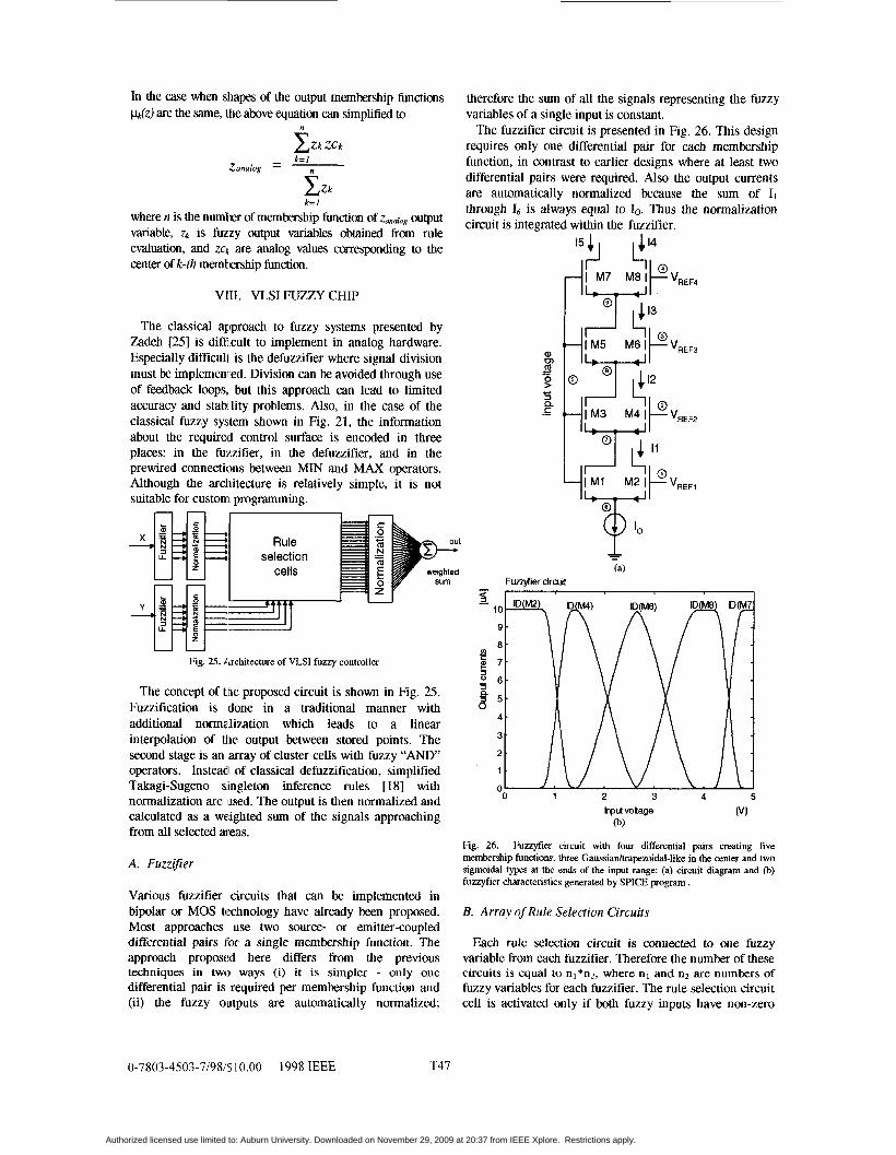
The classical approach to fuzzy systems presented by Zadeh 1251 is difficult to implement in analog hardware. Especially difficuli is the defuzzifier where signal division must be implemenlted. Division can be avoided through use of feedback loops, but this approach can lead to limited accuracy and stabdity problems. Also, in the case of the classical fuzzy system shown in Fig. 21, the information about the required control surface is encoded in three places: in the fuzzifier, in the defuzzifier, and in the prewired connections between MIN and MAX operators. Although the architecture is relatively simple, it is not suitable for custom programming.

J U

u u Fig. 25. Architecture of VLSI fuzzy controller

The concept of the proposed circuit is shown in Fig. 25. Fuzzification is done in a traditional manner with additional normadization which leads to a linear interpolation of the output between stored points. The second stage is an array of cluster cells with fuzzy “AND” operators. Instead of classical defuzzification, simplified Takagi-Sugeno singleton inference rules 181 with normalization are used. The output is then normalized and calculated as a weighted sum of the signals approaching from all selected atas.

A. Fuuifier

Various fuzzifier circuits that can be implemented in bipolar or MOS technology have already been proposed. Most approaches use two source- or emitter-coupled differential pairs lor a single membership function. The approach proposed here differs from the previous techniques in two ways (i) it is simpler - only one differential pair is required per membership function and (ii) the fuzzy outputs are automatically normalized;

therefore the sum of all the signals representing the fuzzy variables of a single input is constant.

The fuzzifier circuit is presented in Fig. 26. This design requires only one differential pair for each membership function, in contrast to earlier designs where at least two differential pairs were required. Also the output currents are automatically normalized because the sum of I1 through I6 is always equal to IO. Thus the normalization circuit is integrated within the fuzzifier.

C .- :I: D

1, (a)

Fuzzyfier circuit

0 1 2 3 4 5

Input voltage VI (b)

Fig. 26. Fuzzyfier circuit with four differential pairs creating five membership functions: three Gaussiadtrapezoidal-like in the center and two sigmoidal types at the ends of the input range: (a) circuit diagram and (b) fuzzyfier characteristics generated by SPICE program .

B. Array @Rule Selection Circuits

Each rule selection circuit is connected to one fuzzy variable from each fuzzifier. Therefore the number of these circuits is equal to nl*nz, where nl and n2 are numbers of fuzzy variables for each fuzzifier. The rule selection circuit cell is activated only if both fuzzy inputs have non-zero

0-7803-4503-7/98/$10.00 1998 IEEE T47


values. Due to the specific shapes of the fuzzifier membership functions, where only two membership functions can overlap, a maximum of four cluster cells are active at a time. Although current mode MIN and MAX operators are possible, it is much easier to convert currents from the fuzzifiers into volhges and use the simple rule selection circuits with the fuzzy conjunction (AND) or fuzzy MIN operator.

The voltage on the common node of all sources always follows the highest potential of any of the transistor gates, so it operates as a MAX/OR circuit. However using the negative signal convention (lower voltages for higher signals) this circuit performs the MIN/AND function. This means that the output signal is low only when all inputs are low. A cluster is selected when all fuzzy signals are significantly lower than the positive battery voltage. Selectivity of the circuit increases with larger W/L ratios. Transistor M3 would be required only if three fuzzifier circuits were used with three inputs.

C. Normalization circuit

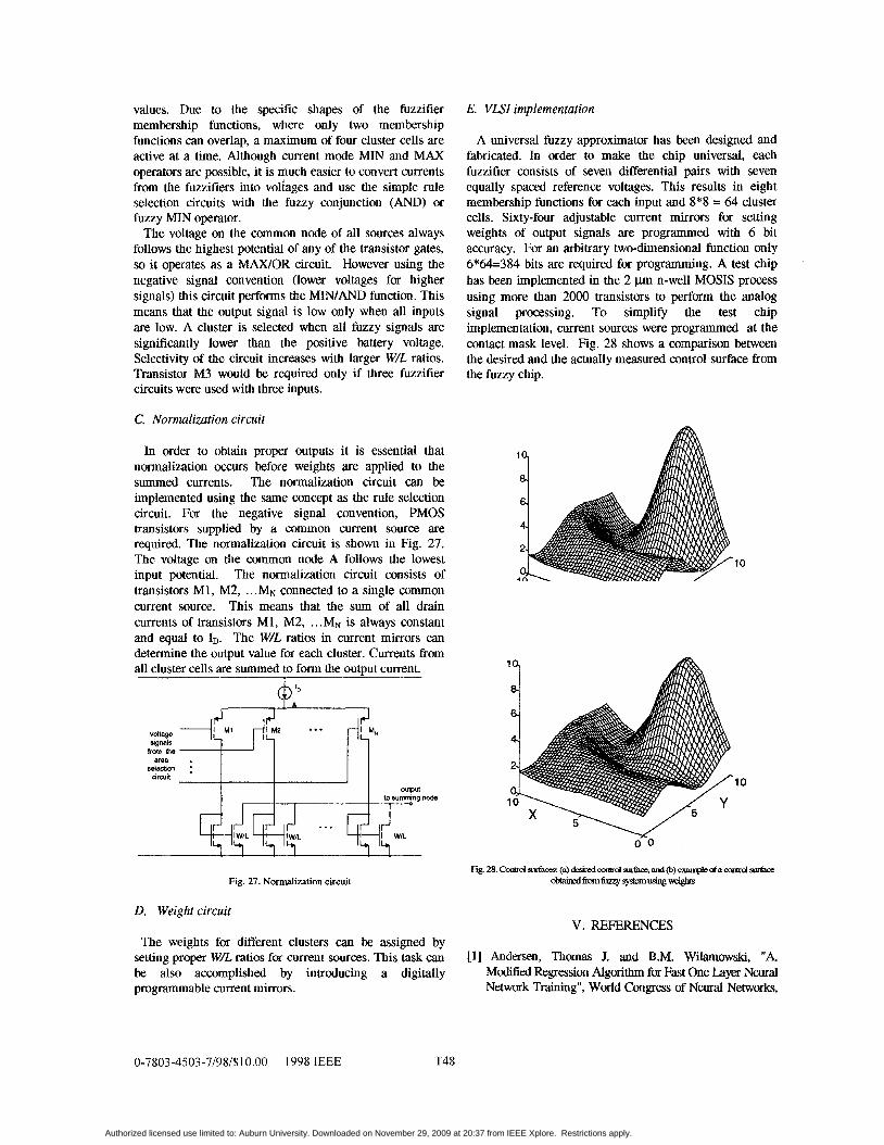
In order to obtain proper outputs it is essential that normalization occurs before weights are applied to the summed currents. The normalization circuit can be implemented using the same concept as the rule selection circuit. For the negative signal convention, PMOS transistors supplied by a common current source are required. The normalization circuit is shown in Fig. 27. The voltage on the common node A follows the lowest input potential. The normalization circuit consists of transistors M1, M2, ... MN connected to a single common current source. This means that the sum of all drain currents of transistors M1, M2, ... MN is always constant and equal to ID. The W/L ratios in current mirrors can determine the output value for each cluster. Currents from all cluster cells are summed to form the output current.

m ID Tn

Fig. 27. Normalization circuit

E. VLSI implementation

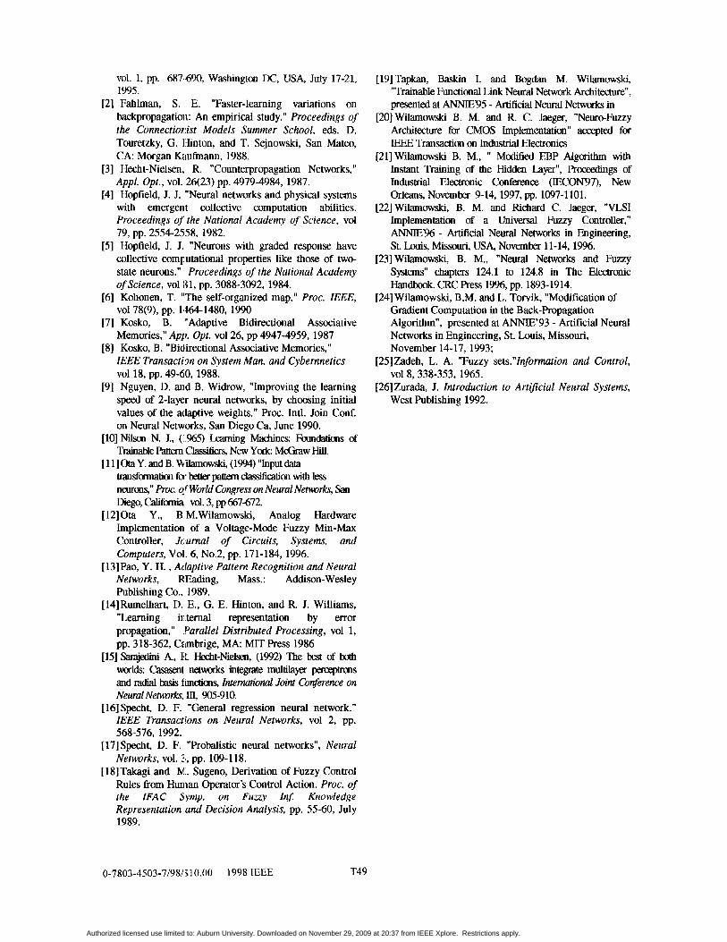
A universal fuzzy approximator has been designed and fabricated. In order to make the chip universal, each fuzzifier consists of seven differential pairs with seven equally spaced reference voltages. This results in eight membership functions for each input and 8*8 = 64 cluster cells. Sixty-four adjustable current mirrors for setting weights of output signals are programmed with 6 bit accuracy. For an arbitrary two-dimensional function only 6*64=384 bits are required for programming. A test chip has been implemented in the 2 p n-well MOSIS process using more than 2000 transistors to perform the analog signal processing. To simplify the test chip implementation, current sources were programmed at the contact mask level. Fig. 28 shows a comparison between the desired and the actually measured control surface from the fuzzy chip.

1

10 4

1

10

1

D. Weight circuit V. REFER.E!NCES

The weights for different clusters can be assigned by setting proper W/L ratios for current sources. This task can be also accomplished by introducing a digitally programmable current mirrors.

0-7803-4503-7/98/$10.00 1998 IEEE T48

[l] Andersen, Thomas J. and B.M. Wilamowski, “A. Modified Regression Algorithm for Fast One Layer Neural Network Training”, World Congress of Neural Networks,


vol. 1, pp. 687.690, Washington DC, USA, July 17-21, 1W5.

[21 Fahlman, S. E. "Faster-learning variations on backpropagation: An empirical study." Proceedings of the Connectioriist Models Summer School, eds. D. Touretzky, G. Ilinton, and T. Sejnowski, San Mateo, CA: Morgan Kaufmann, 1988.

[3] Hecht-Nielsen, R. "Counterpropagation Networks," Appl. Opt., vol. 26(23) pp. 4979-4984, 1987.

[4] Hopfield, J. J. "Neural networks and physical systems with emergent collective computation abilities. Proceedings of the National Academy of Science, vol

[5] Hopfield, J. J. "Neurons with graded response have collective computational properties like those of two- state neurons." Proceedings of the National Academy of Science, ~0181, pp. 3088-3092, 1984.

[6] Kohonen, T. "The self-organized map," Proc. IEEE,

[7] Kosko, B. "Adaptive Bidirectional Associative Memories," App. Opt. vol26, pp 4947-4959, 1987

[8] Kosko, B. "Bidirectional Associative Memories," IEEE Transaction on System Man, and Cybernnetics

[9] Nguyen, D. and B. Widrow, "Improving the learning speed of 2-layer neural networks, by choosing initial values of the adaptive weights." Roc. Intl. Join Conf. on Neural Networks, San Diego Ca, June 1990.

[lo] Nilson N. J., (1%5) Leaming Machines: Foundations of Trainable Paaem chssifim New York: McGraw Hill.

[ l l ] O t a Y . a n d B . V v ' i i ~ (1994)"Inputdata

79, pp. 2554-2558, 1982.

VOI 78(9), pp. 1464-1480, 1990

V O ~ 18, pp. 49-60, 1988.

transformation &Ybetteapattesnclass~cation with less neurons,'' Proc. qf World Congress on Neural Nemrks, San Diego, califomia vol. 3, pp 667-672.

[12]0ta Y., B M.Wilamowski, Analog Hardware Implementation of a Voltage-Mode Fuzzy Min-Max Controller, Journal of Circuits, Systems, and Computers, Vol. 6, No.2, pp. 171-184, 1996.

[13]Pao, Y. H. , Adaptive Pattern Recognition and Neural Networks, REading, Mass.: Addison-Wesley Publishing Co., 1989.

[14]Rumelhart, D. E., G. E. Hinton, and R. J. Williams, "Learning internal representation by error propagation," Parallel Distributed Processing, vol 1, pp. 318-362, Cambrige, MA: MIT Press 1986

[15] sarajedrni A., EL zkxht-Nielsen, (1992) The best of both worlds: Casasent networks integrate multilayer p e " s and radial basis functions, Iruematwmd Joint Cbnference on Neural Nemrks, IlI, 905-910.

[ 161 Specht, D. F. "General regression neural network." IEEE Transactions on Neural Networks, vol 2, pp.

[ 171 Specht, D. F. "Probalistic neural networks", Neural Networks, vol. 3, pp. 109-118.

[18]Takagi and MI. Sugeno, Derivation of Fuzzy Control Rules from Human Operator's Control Action. Proc. of the IFAC Symp. on Fuzzy In$ Knowledge Representation and Decision Analysis, pp. 55-60, July 1989.

568-576, 1992.

[19]Tapkan, Baskin I. and Bog& M. Wilamowski, "Trainable Functional Link Neural Network Architecture", presented at ANNIE95 - Artificial Neural Networks in

[20]Wilamowski B. M. and R C. Jaeger, "Neuro-Fuzzy Architecture for CMOS Implementation" accepted for IEEE Transaction on Industrial Electronics

[21]Wilamowski B. M., " Modified EBP Algorithm with Instant Training of the Hidden Layer", proceedings of Industrial Electronic Conference (IECON97), New Orleans, November 9-14, 1997, pp. 1097-1101.

[22]Wilamowski, B. M. and Richard C. Jaeger, "VLSI Implementation of a Universal Fuzzy Controller," ANNIE96 - Artificial Neural Networks in Engineering, St. Louis, Missouri, USA, November 11-14,1996.

[23]Wilamowski, B. M., "Neural Networks and Fuzzy Systems" chapters 124.1 to 124.8 in The Electronic HandW. CRC Press 1996, pp. 1893-1914.

[24] Wilamowski, B.M. and L. Torvik, "Modification of Gradient Computation in the Back-Propagation Algorithm", presented at ANNIE'93 - Artificial Neural Networks in Engineering, St. Louis, Missouri, November 14-17,1993;

[25] Zadeh, L. A. "Fuzzy sets."lnformution and Control,

[26] Zurada, J. Introduction to Artificial Neural Systems, V O ~ 8, 338-353, 1965.

West Publishing 1992.

0-7803-4503-7/98/$10.00 1998 lEEE T49


Documents

Neuro-fuzzy Systems and Their Applicationswilambm/pap/1999/new Neuro-fuzzy Systems … · technological re capable of rep1 experience. The concept underlining thei and comparisoi