Embed Size (px)
Citation preview
N E U R O - F U Z Z YT E C H N I Q U E S TO
O P T I M I Z E A N F P G AE M B E D D E D C O N T R O L L E RF O R R O B OT N AV I G AT I O Ni . baturone1 , a. gersnoviez2 and a. barriga1
contents1 Introduction 4
2 The first design of the FPGA controller 5
2.1 The navigation algorithm . . . . . . . . . . . . . . . . . . . . . 5
2.2 Very close obstacles . . . . . . . . . . . . . . . . . . . . . . . . . 7
2.3 Close obstacles . . . . . . . . . . . . . . . . . . . . . . . . . . . 8
2.4 Obstacle avoidance . . . . . . . . . . . . . . . . . . . . . . . . . 9
2.5 Navigation toward the goal . . . . . . . . . . . . . . . . . . . . 9
3 Optimizing the design with neuro-fuzzy techniques 10
3.1 Very close obstacles . . . . . . . . . . . . . . . . . . . . . . . . . 10
3.2 Close obstacles . . . . . . . . . . . . . . . . . . . . . . . . . . . 11
3.3 Obstacle avoidance . . . . . . . . . . . . . . . . . . . . . . . . . 12
3.4 Navigation toward the goal . . . . . . . . . . . . . . . . . . . . 13
4 Results and discussion 15
4.1 Simulation and experimental results . . . . . . . . . . . . . . . 15
4.2 Implementation results . . . . . . . . . . . . . . . . . . . . . . . 17
4.3 Discussion . . . . . . . . . . . . . . . . . . . . . . . . . . . . . . 19
5 Conclusions 20
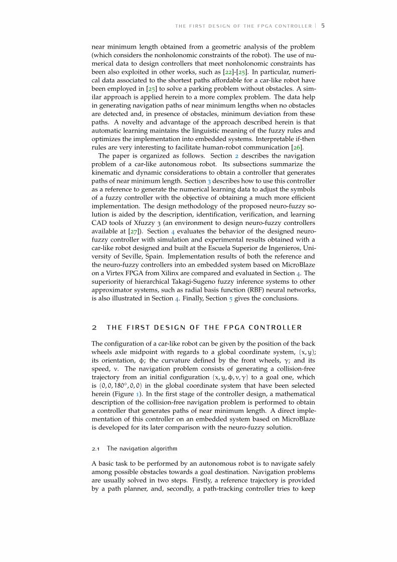
list of figuresFigure 1 The navigation problem . . . . . . . . . . . . . . . . . 6
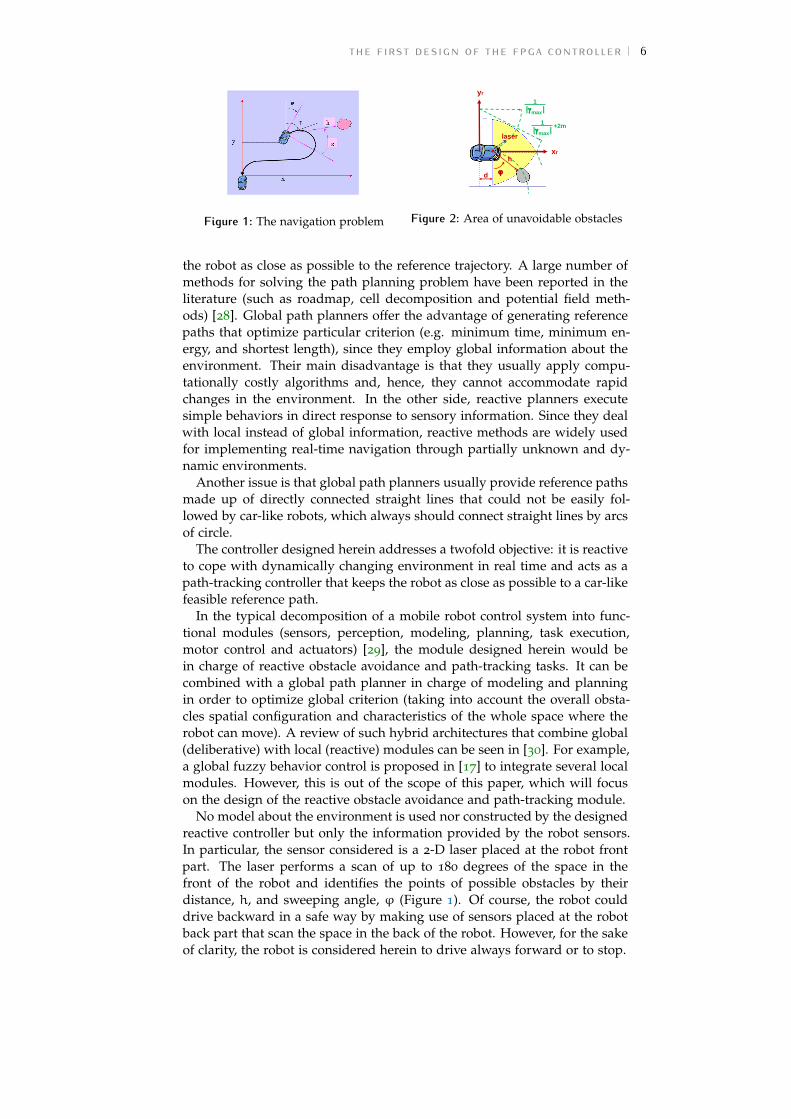
Figure 2 Area of unavoidable obstacles . . . . . . . . . . . . . . 6
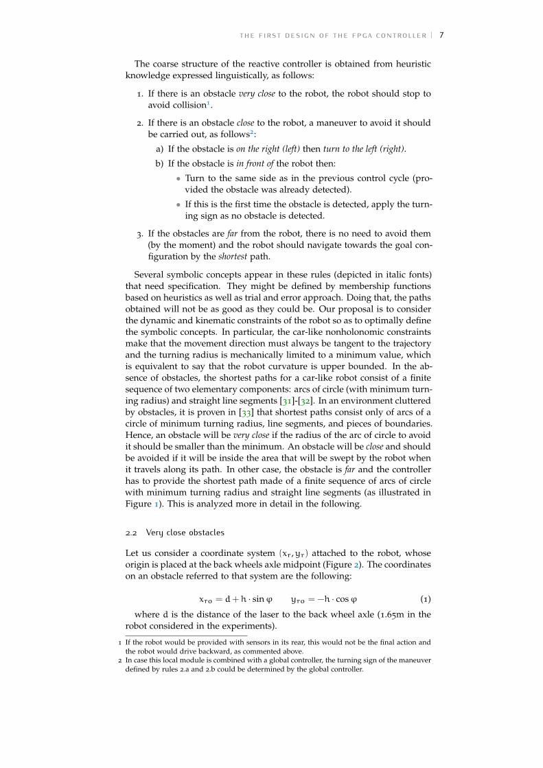
Figure 3 (a) Area of close obstacles. (b) Transformation be-tween coordinate systems (xr,yr) and (xR,yR). . . . 8
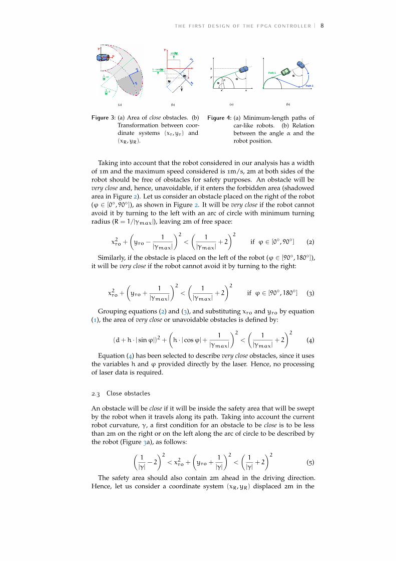
Figure 4 (a) Minimum-length paths of car-like robots. (b) Re-lation between the angle α and the robot position. . . 8
Figure 5 (a) Structure of the fuzzy classifier for very close ob-stacles. (b) The gray area is the area of very close ob-stacles according to (4). (c) Result provided by thefuzzy classifier. . . . . . . . . . . . . . . . . . . . . . . 11
1
List of Tables 2
Figure 6 (a) Hierarchical system to classify obstacles as closeor not. (b) Maximum value of h, hmax, of obstaclesconsidering as close according to (5)-(7). (c) Approxi-mation of hmax provided by the fuzzy classifier. . . . 11
Figure 7 Input-output behavior of the rule base Distance inFigure 6a. . . . . . . . . . . . . . . . . . . . . . . . . . . 12
Figure 8 (a) Curvature to avoid obstacles according to (9). (b)25 rules extracted by Wang-Mendel algorithm with aregular 5x5 grid. (c) The 5x5 grid is adjusted to thedata by supervised learning. . . . . . . . . . . . . . . . 12
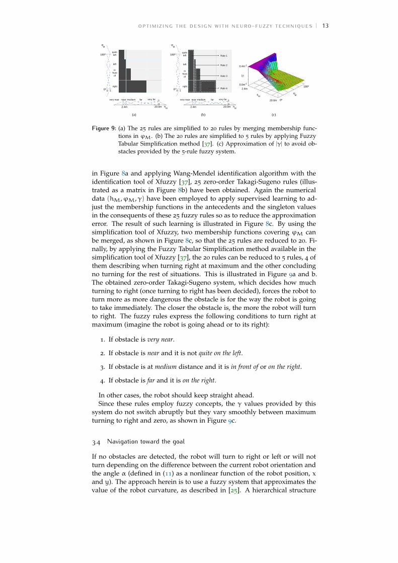
Figure 9 (a) The 25 rules are simplified to 20 rules by mergingmembership functions in ϕM. (b) The 20 rules aresimplified to 5 rules by applying Fuzzy Tabular Sim-plification method [37]. (c) Approximation of |γ| toavoid obstacles provided by the 5-rule fuzzy system. 13
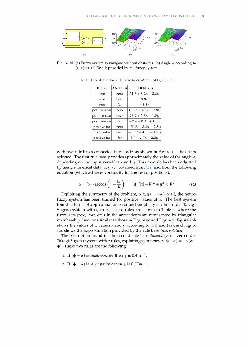
Figure 10 (a) Fuzzy system to navigate without obstacles. (b)Angle α according to (10)-(11). (c) Result providedby the fuzzy system. . . . . . . . . . . . . . . . . . . . 14
Figure 11 Simulation results of navigation with and withoutobstacles, provided by initial and neuro-fuzzy (op-timized) controllers (axis units are in meters). . . . . 15
Figure 12 Simulation results of navigation with an emergentmoving obstacle. . . . . . . . . . . . . . . . . . . . . . . 16
Figure 13 Experimental results of navigation with and withoutobstacles obtained with the neuro-fuzzy controller(axis units are in meters). . . . . . . . . . . . . . . . . 16
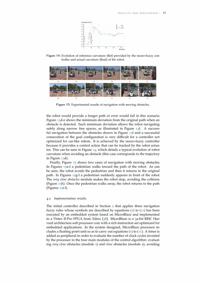
Figure 14 Evolution of reference curvature (Ref) provided bythe neuro-fuzzy controller and actual curvature (Real)of the robot. . . . . . . . . . . . . . . . . . . . . . . . . 17
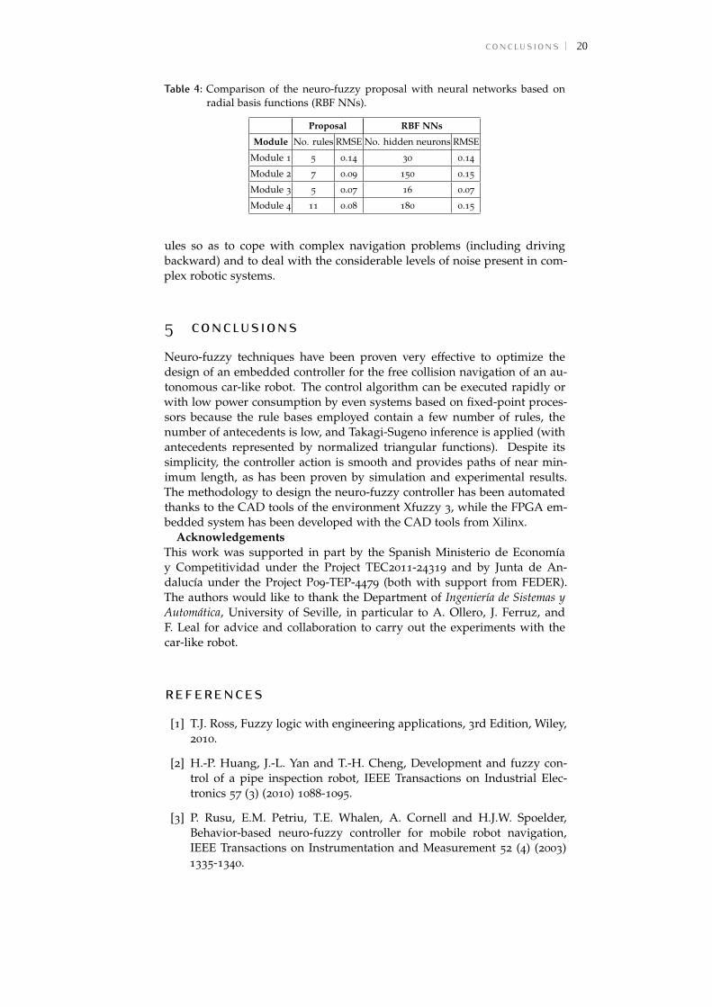
Figure 15 Experimental results of navigation with moving ob-stacles. . . . . . . . . . . . . . . . . . . . . . . . . . . . 17
list of tablesTable 1 Rules in the rule base Interpolation of Figure 10 . . . . . . . 14
Table 2 Number of clock cycles required by the initial and opti-mized (neuro-fuzzy) embedded controllers . . . . . . . . . 18
Table 3 Computation time (in seconds) of embedded controllers us-ing 50MHz of working frequency . . . . . . . . . . . . . . 18
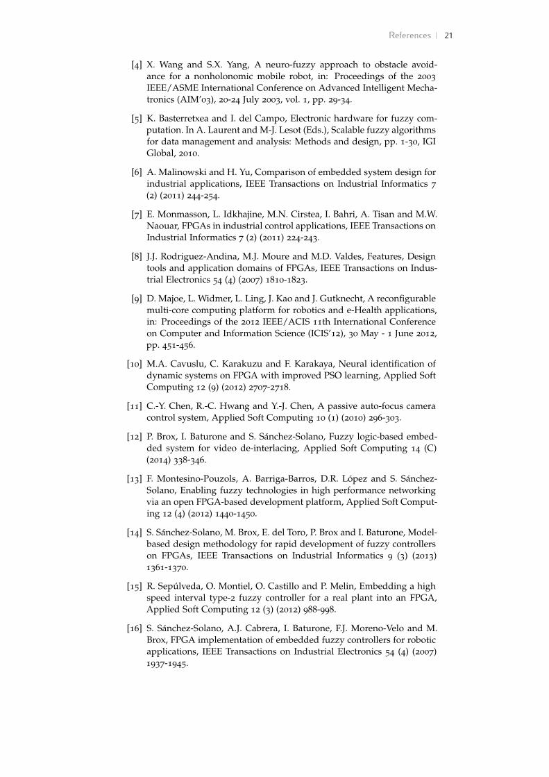
Table 4 Comparison of the neuro-fuzzy proposal with neural net-works based on radial basis functions (RBF NNs). . . . . . 20
abstractThis paper describes how low-cost embedded controllers for robot naviga-tion can be obtained by using a small number of if-then rules (exploiting theconnection in cascade of rule bases) that apply Takagi-Sugeno fuzzy infer-ence method and employ fuzzy sets represented by normalized triangularfunctions. The rules comprise heuristic and fuzzy knowledge together withnumerical data obtained from a geometric analysis of the control problem
List of Tables 3
that considers the kinematic and dynamic constraints of the robot. Numer-ical data allow tuning the fuzzy symbols used in the rules to optimize thecontroller performance. From the implementation point of view, very fewcomputational and memory resources are required: standard logical, addi-tion, and multiplication operations and a few data that can be representedby integer values. This is illustrated with the design of a controller for thesafe navigation of an autonomous car-like robot among possible obstacles to-wards a goal configuration. Implementation results of an FPGA embeddedsystem based on a general-purpose soft processor confirm that percentagereduction in clock cycles is drastic thanks to applying the proposed neuro-fuzzy techniques. Simulation and experimental results obtained with therobot confirm the efficiency of the controller designed. Design methodol-ogy has been supported by the CAD tools of the environment Xfuzzy 3 andby the Embedded System Tools from Xilinx.
* 1Dept. de Electrónica y Electromagnetismo, Univ. of Seville, and the Instituto de Microelectrónica deSevilla (IMSE-CNM-CSIC), Seville (Spain)1 2Dept. de Arquitectura de Computadores, Electrónica y Tecnología Electrónica, Univ. of Cordoba,Cordoba (Spain)
introduction 4
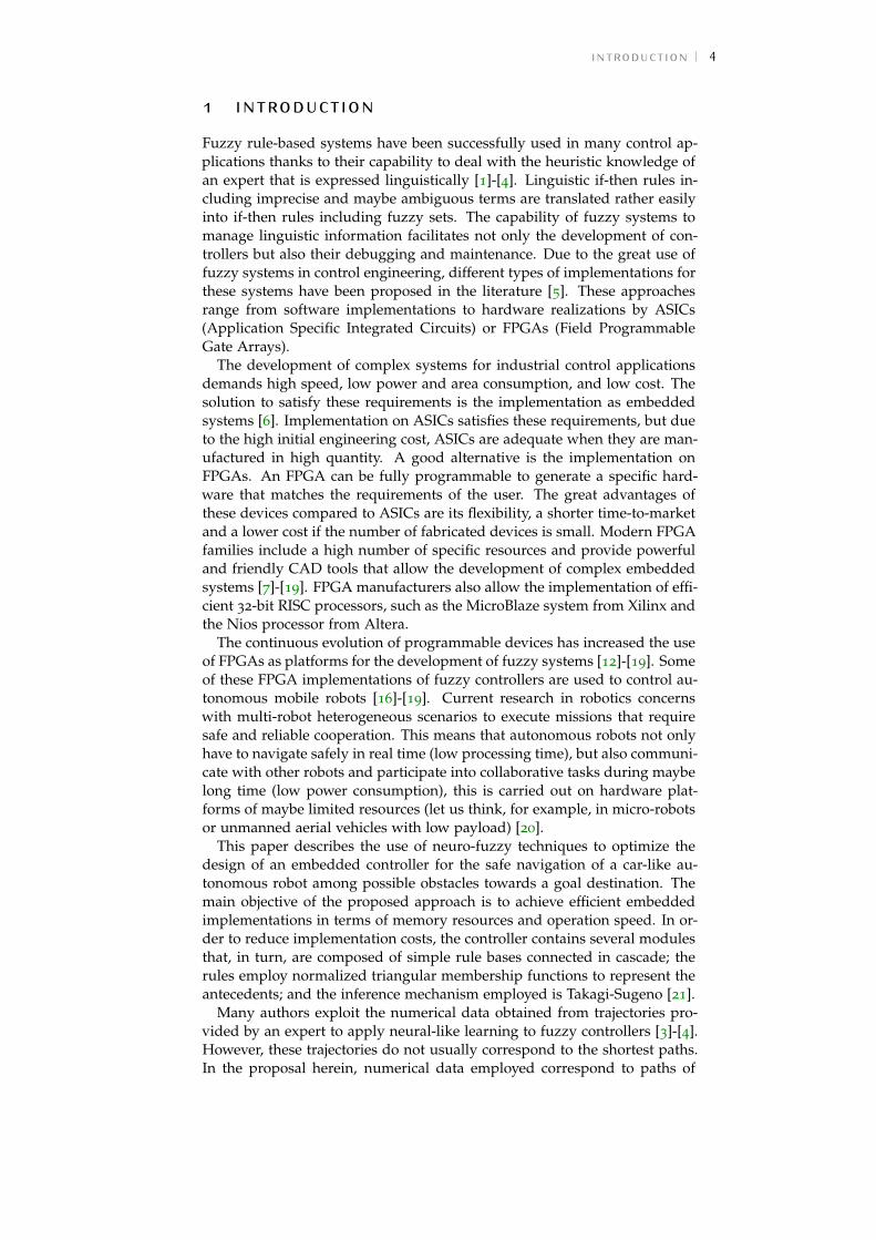
1 introductionFuzzy rule-based systems have been successfully used in many control ap-plications thanks to their capability to deal with the heuristic knowledge ofan expert that is expressed linguistically [1]-[4]. Linguistic if-then rules in-cluding imprecise and maybe ambiguous terms are translated rather easilyinto if-then rules including fuzzy sets. The capability of fuzzy systems tomanage linguistic information facilitates not only the development of con-trollers but also their debugging and maintenance. Due to the great use offuzzy systems in control engineering, different types of implementations forthese systems have been proposed in the literature [5]. These approachesrange from software implementations to hardware realizations by ASICs(Application Specific Integrated Circuits) or FPGAs (Field ProgrammableGate Arrays).
The development of complex systems for industrial control applicationsdemands high speed, low power and area consumption, and low cost. Thesolution to satisfy these requirements is the implementation as embeddedsystems [6]. Implementation on ASICs satisfies these requirements, but dueto the high initial engineering cost, ASICs are adequate when they are man-ufactured in high quantity. A good alternative is the implementation onFPGAs. An FPGA can be fully programmable to generate a specific hard-ware that matches the requirements of the user. The great advantages ofthese devices compared to ASICs are its flexibility, a shorter time-to-marketand a lower cost if the number of fabricated devices is small. Modern FPGAfamilies include a high number of specific resources and provide powerfuland friendly CAD tools that allow the development of complex embeddedsystems [7]-[19]. FPGA manufacturers also allow the implementation of effi-cient 32-bit RISC processors, such as the MicroBlaze system from Xilinx andthe Nios processor from Altera.
The continuous evolution of programmable devices has increased the useof FPGAs as platforms for the development of fuzzy systems [12]-[19]. Someof these FPGA implementations of fuzzy controllers are used to control au-tonomous mobile robots [16]-[19]. Current research in robotics concernswith multi-robot heterogeneous scenarios to execute missions that requiresafe and reliable cooperation. This means that autonomous robots not onlyhave to navigate safely in real time (low processing time), but also communi-cate with other robots and participate into collaborative tasks during maybelong time (low power consumption), this is carried out on hardware plat-forms of maybe limited resources (let us think, for example, in micro-robotsor unmanned aerial vehicles with low payload) [20].
This paper describes the use of neuro-fuzzy techniques to optimize thedesign of an embedded controller for the safe navigation of a car-like au-tonomous robot among possible obstacles towards a goal destination. Themain objective of the proposed approach is to achieve efficient embeddedimplementations in terms of memory resources and operation speed. In or-der to reduce implementation costs, the controller contains several modulesthat, in turn, are composed of simple rule bases connected in cascade; therules employ normalized triangular membership functions to represent theantecedents; and the inference mechanism employed is Takagi-Sugeno [21].
Many authors exploit the numerical data obtained from trajectories pro-vided by an expert to apply neural-like learning to fuzzy controllers [3]-[4].However, these trajectories do not usually correspond to the shortest paths.In the proposal herein, numerical data employed correspond to paths of
the first design of the fpga controller 5
near minimum length obtained from a geometric analysis of the problem(which considers the nonholonomic constraints of the robot). The use of nu-merical data to design controllers that meet nonholonomic constraints hasbeen also exploited in other works, such as [22]-[25]. In particular, numeri-cal data associated to the shortest paths affordable for a car-like robot havebeen employed in [25] to solve a parking problem without obstacles. A sim-ilar approach is applied herein to a more complex problem. The data helpin generating navigation paths of near minimum lengths when no obstaclesare detected and, in presence of obstacles, minimum deviation from thesepaths. A novelty and advantage of the approach described herein is thatautomatic learning maintains the linguistic meaning of the fuzzy rules andoptimizes the implementation into embedded systems. Interpretable if-thenrules are very interesting to facilitate human-robot communication [26].
The paper is organized as follows. Section 2 describes the navigationproblem of a car-like autonomous robot. Its subsections summarize thekinematic and dynamic considerations to obtain a controller that generatespaths of near minimum length. Section 3 describes how to use this controlleras a reference to generate the numerical learning data to adjust the symbolsof a fuzzy controller with the objective of obtaining a much more efficientimplementation. The design methodology of the proposed neuro-fuzzy so-lution is aided by the description, identification, verification, and learningCAD tools of Xfuzzy 3 (an environment to design neuro-fuzzy controllersavailable at [27]). Section 4 evaluates the behavior of the designed neuro-fuzzy controller with simulation and experimental results obtained with acar-like robot designed and built at the Escuela Superior de Ingenieros, Uni-versity of Seville, Spain. Implementation results of both the reference andthe neuro-fuzzy controllers into an embedded system based on MicroBlazeon a Virtex FPGA from Xilinx are compared and evaluated in Section 4. Thesuperiority of hierarchical Takagi-Sugeno fuzzy inference systems to otherapproximator systems, such as radial basis function (RBF) neural networks,is also illustrated in Section 4. Finally, Section 5 gives the conclusions.
2 the first design of the fpga controllerThe configuration of a car-like robot can be given by the position of the backwheels axle midpoint with regards to a global coordinate system, (x,y);its orientation, φ; the curvature defined by the front wheels, γ; and itsspeed, v. The navigation problem consists of generating a collision-freetrajectory from an initial configuration (x,y,φ, v,γ) to a goal one, whichis (0, 0, 180◦, 0, 0) in the global coordinate system that have been selectedherein (Figure 1). In the first stage of the controller design, a mathematicaldescription of the collision-free navigation problem is performed to obtaina controller that generates paths of near minimum length. A direct imple-mentation of this controller on an embedded system based on MicroBlazeis developed for its later comparison with the neuro-fuzzy solution.
2.1 The navigation algorithm
A basic task to be performed by an autonomous robot is to navigate safelyamong possible obstacles towards a goal destination. Navigation problemsare usually solved in two steps. Firstly, a reference trajectory is providedby a path planner, and, secondly, a path-tracking controller tries to keep
the first design of the fpga controller 6
Figure 1: The navigation problem
laser
d
h
j
+2m
yr
xr
1
|g | max
1
|g | max
Figure 2: Area of unavoidable obstacles
the robot as close as possible to the reference trajectory. A large number ofmethods for solving the path planning problem have been reported in theliterature (such as roadmap, cell decomposition and potential field meth-ods) [28]. Global path planners offer the advantage of generating referencepaths that optimize particular criterion (e.g. minimum time, minimum en-ergy, and shortest length), since they employ global information about theenvironment. Their main disadvantage is that they usually apply compu-tationally costly algorithms and, hence, they cannot accommodate rapidchanges in the environment. In the other side, reactive planners executesimple behaviors in direct response to sensory information. Since they dealwith local instead of global information, reactive methods are widely usedfor implementing real-time navigation through partially unknown and dy-namic environments.
Another issue is that global path planners usually provide reference pathsmade up of directly connected straight lines that could not be easily fol-lowed by car-like robots, which always should connect straight lines by arcsof circle.
The controller designed herein addresses a twofold objective: it is reactiveto cope with dynamically changing environment in real time and acts as apath-tracking controller that keeps the robot as close as possible to a car-likefeasible reference path.
In the typical decomposition of a mobile robot control system into func-tional modules (sensors, perception, modeling, planning, task execution,motor control and actuators) [29], the module designed herein would bein charge of reactive obstacle avoidance and path-tracking tasks. It can becombined with a global path planner in charge of modeling and planningin order to optimize global criterion (taking into account the overall obsta-cles spatial configuration and characteristics of the whole space where therobot can move). A review of such hybrid architectures that combine global(deliberative) with local (reactive) modules can be seen in [30]. For example,a global fuzzy behavior control is proposed in [17] to integrate several localmodules. However, this is out of the scope of this paper, which will focuson the design of the reactive obstacle avoidance and path-tracking module.
No model about the environment is used nor constructed by the designedreactive controller but only the information provided by the robot sensors.In particular, the sensor considered is a 2-D laser placed at the robot frontpart. The laser performs a scan of up to 180 degrees of the space in thefront of the robot and identifies the points of possible obstacles by theirdistance, h, and sweeping angle, ϕ (Figure 1). Of course, the robot coulddrive backward in a safe way by making use of sensors placed at the robotback part that scan the space in the back of the robot. However, for the sakeof clarity, the robot is considered herein to drive always forward or to stop.
the first design of the fpga controller 7
The coarse structure of the reactive controller is obtained from heuristicknowledge expressed linguistically, as follows:
1. If there is an obstacle very close to the robot, the robot should stop toavoid collision1.
2. If there is an obstacle close to the robot, a maneuver to avoid it shouldbe carried out, as follows2:
a) If the obstacle is on the right (left) then turn to the left (right).
b) If the obstacle is in front of the robot then:
• Turn to the same side as in the previous control cycle (pro-vided the obstacle was already detected).
• If this is the first time the obstacle is detected, apply the turn-ing sign as no obstacle is detected.
3. If the obstacles are far from the robot, there is no need to avoid them(by the moment) and the robot should navigate towards the goal con-figuration by the shortest path.
Several symbolic concepts appear in these rules (depicted in italic fonts)that need specification. They might be defined by membership functionsbased on heuristics as well as trial and error approach. Doing that, the pathsobtained will not be as good as they could be. Our proposal is to considerthe dynamic and kinematic constraints of the robot so as to optimally definethe symbolic concepts. In particular, the car-like nonholonomic constraintsmake that the movement direction must always be tangent to the trajectoryand the turning radius is mechanically limited to a minimum value, whichis equivalent to say that the robot curvature is upper bounded. In the ab-sence of obstacles, the shortest paths for a car-like robot consist of a finitesequence of two elementary components: arcs of circle (with minimum turn-ing radius) and straight line segments [31]-[32]. In an environment clutteredby obstacles, it is proven in [33] that shortest paths consist only of arcs of acircle of minimum turning radius, line segments, and pieces of boundaries.Hence, an obstacle will be very close if the radius of the arc of circle to avoidit should be smaller than the minimum. An obstacle will be close and shouldbe avoided if it will be inside the area that will be swept by the robot whenit travels along its path. In other case, the obstacle is far and the controllerhas to provide the shortest path made of a finite sequence of arcs of circlewith minimum turning radius and straight line segments (as illustrated inFigure 1). This is analyzed more in detail in the following.
2.2 Very close obstacles
Let us consider a coordinate system (xr,yr) attached to the robot, whoseorigin is placed at the back wheels axle midpoint (Figure 2). The coordinateson an obstacle referred to that system are the following:
xro = d+ h · sinϕ yro = −h · cosϕ (1)
where d is the distance of the laser to the back wheel axle (1.65m in therobot considered in the experiments).
1 If the robot would be provided with sensors in its rear, this would not be the final action andthe robot would drive backward, as commented above.
2 In case this local module is combined with a global controller, the turning sign of the maneuverdefined by rules 2.a and 2.b could be determined by the global controller.
the first design of the fpga controller 8
yr
xr
|g|
1 +2
|g|
1 -2
2g
2g
sin(2g)
g
g
1 - cos(2g)
g
yr
xr
1
(a) (b)
Figure 3: (a) Area of close obstacles. (b)Transformation between coor-dinate systems (xr,yr) and(xR,yR).
a
Path 1
Path 2
x x’
y
y’ a
a
R
(a) (b)
Figure 4: (a) Minimum-length paths ofcar-like robots. (b) Relationbetween the angle α and therobot position.
Taking into account that the robot considered in our analysis has a widthof 1m and the maximum speed considered is 1m/s, 2m at both sides of therobot should be free of obstacles for safety purposes. An obstacle will bevery close and, hence, unavoidable, if it enters the forbidden area (shadowedarea in Figure 2). Let us consider an obstacle placed on the right of the robot(ϕ ∈ [0◦, 90◦]), as shown in Figure 2. It will be very close if the robot cannotavoid it by turning to the left with an arc of circle with minimum turningradius (R = 1/|γmax|), leaving 2m of free space:
x2ro +
(yro −
1
|γmax|
)2<
(1
|γmax|+ 2
)2if ϕ ∈ [0◦, 90◦] (2)
Similarly, if the obstacle is placed on the left of the robot (ϕ ∈ [90◦, 180◦]),it will be very close if the robot cannot avoid it by turning to the right:
x2ro +
(yro +
1
|γmax|
)2<
(1
|γmax|+ 2
)2if ϕ ∈ [90◦, 180◦] (3)
Grouping equations (2) and (3), and substituting xro and yro by equation(1), the area of very close or unavoidable obstacles is defined by:
(d+ h · | sinϕ|)2 +(h · | cosϕ|+
1
|γmax|
)2<
(1
|γmax|+ 2
)2(4)
Equation (4) has been selected to describe very close obstacles, since it usesthe variables h and ϕ provided directly by the laser. Hence, no processingof laser data is required.
2.3 Close obstacles
An obstacle will be close if it will be inside the safety area that will be sweptby the robot when it travels along its path. Taking into account the currentrobot curvature, γ, a first condition for an obstacle to be close is to be lessthan 2m on the right or on the left along the arc of circle to be described bythe robot (Figure 3a), as follows:(
1
|γ|− 2
)2< x2ro +
(yro +
1
|γ|
)2<
(1
|γ|+ 2
)2(5)
The safety area should also contain 2m ahead in the driving direction.Hence, let us consider a coordinate system (xR,yR) displaced 2m in the
the first design of the fpga controller 9
driving direction and rotated an angle of 2γ with respect to the coordinatesystem (xr,yr), as illustrated in Figure 3b. The coordinates of an obstaclereferred to this system are the following:
xRo =(xro −
sin2γγ
)cos 2γ−
(yro +
1−cos2γγ
)sin 2γ
yRo =(xro −
sin2γγ
)sin 2γ+
(yro +
1−cos2γγ
)cos 2γ
(6)
A second condition for an obstacle to be close and, hence, to be avoidedis that it becomes a very close obstacle in the future (dark shadowed areain Figure 3a). This condition is easier to be expressed in the coordinatesystem (xR,yR). Similarly to equations (2) and (3), it will be very close iftheir position with regards to the displaced and rotated coordinate systemverifies that:
x2Ro +
(yRo +
1
|γmax|
)2<
(1
|γmax|+ 2
)2(7)
Finally, the third condition for a close obstacle is that, currently, it is notvery close and, hence, it does not verify equation (4).
2.4 Obstacle avoidance
The minimum magnitude of the curvature to avoid an obstacle identified asclose is determined by the closest point of that obstacle (whose coordinateswill be named hM and ϕM herein). Taking into account that a referencecurvature is not adopted instantaneously by the robot but has a delay, a 4-msafety corridor has been considered for selecting the minimum value of thecurvature. With such selection, the dynamic features of the robot consideredin the experiments allow the 2-m width corridor free of obstacles. Hence,the minimum magnitude of the curvature (similarly to equation (4)) is givenby:
(d+ hM · | sinϕM|)2 +
(hM · | cosϕM|+
1
|γ|
)2=
(1
|γ|+ 4
)2(8)
From the formula above, the value of |γ| can be obtained as:
|γ| =8− 2hM · | cosϕM|
d2 + h2M + 2hM · d · | sinϕM|− 16(9)
The sign of the curvature when an obstacle is avoided is given by thesecond if-then rule explained in Subsection 2.1 (the criterion adopted is that|γ| = γ, in the case of turning to the right, and |γ| = −γ, in the case ofturning to the left).
2.5 Navigation toward the goal
If there are no obstacles, the robot should navigate toward the goal (0,0,180◦,0,0)
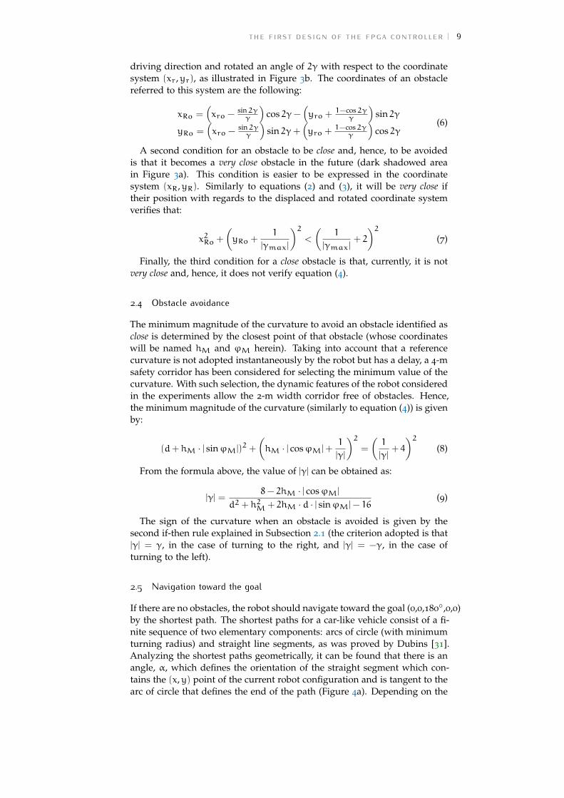
by the shortest path. The shortest paths for a car-like vehicle consist of a fi-nite sequence of two elementary components: arcs of circle (with minimumturning radius) and straight line segments, as was proved by Dubins [31].Analyzing the shortest paths geometrically, it can be found that there is anangle, α, which defines the orientation of the straight segment which con-tains the (x,y) point of the current robot configuration and is tangent to thearc of circle that defines the end of the path (Figure 4a). Depending on the
optimizing the design with neuro-fuzzy techniques 10
difference between this angle and the current robot orientation, the robotwill turn to right or left or will not turn. The value of the angle α dependson x and y as follows (as can be seen in Figure 4b):
tanα = x−x′
y−y′ =x−(R−R·cosα)y−R·sinα
with (|x|− R)2 + y2 > R2(10)
where R is the minimum turning radius.If the formula above is elaborated, the value of α can be obtained as
follows:
α = (x) · arccos
(R(R− |x|) + y
√x2 + y2 − 2R|x|
x2 + y2 − 2R|x|+ R2
)(11)
3 optimizing the design with neuro-fuzzytechniques
The direct implementation of equations (1) to (11) requires trigonometricfunctions (sin, cos and arccos), square root, and division. As discussed inSection 4, such equations are computationally costly for FPGA embeddedcontrollers (when carried out by MicroBlaze processor using software rou-tines). One solution is to accelerate by hardware the computation of suchfunctions. Another approach to alleviate this cost is to simplify the equa-tions to compute the safety areas. The latter is the approach proposed in[34], which is a little conservative solution that constructs a polygonal over-approximation of such areas and checks the emptiness of the constructedconvex polygon with any obstacle by solving a linear programming problem.The novel approach proposed herein is to employ neuro-fuzzy techniquesto simplify the computation of all the equations not only of the safety areas,and, in the case of safety areas, not providing a coarse over-approximationbut a finer approximation. This is analyzed more in detail in the following.
3.1 Very close obstacles
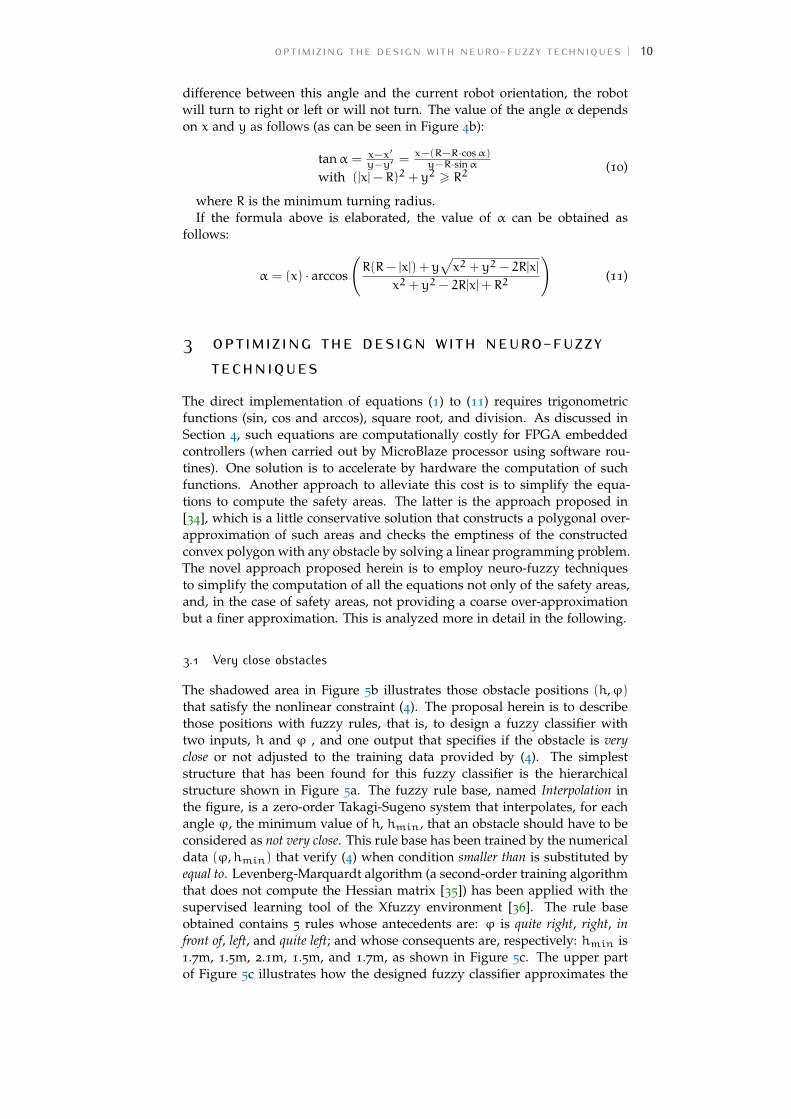
The shadowed area in Figure 5b illustrates those obstacle positions (h,ϕ)that satisfy the nonlinear constraint (4). The proposal herein is to describethose positions with fuzzy rules, that is, to design a fuzzy classifier withtwo inputs, h and ϕ , and one output that specifies if the obstacle is veryclose or not adjusted to the training data provided by (4). The simpleststructure that has been found for this fuzzy classifier is the hierarchicalstructure shown in Figure 5a. The fuzzy rule base, named Interpolation inthe figure, is a zero-order Takagi-Sugeno system that interpolates, for eachangle ϕ, the minimum value of h, hmin, that an obstacle should have to beconsidered as not very close. This rule base has been trained by the numericaldata (ϕ,hmin) that verify (4) when condition smaller than is substituted byequal to. Levenberg-Marquardt algorithm (a second-order training algorithmthat does not compute the Hessian matrix [35]) has been applied with thesupervised learning tool of the Xfuzzy environment [36]. The rule baseobtained contains 5 rules whose antecedents are: ϕ is quite right, right, infront of, left, and quite left; and whose consequents are, respectively: hmin is1.7m, 1.5m, 2.1m, 1.5m, and 1.7m, as shown in Figure 5c. The upper partof Figure 5c illustrates how the designed fuzzy classifier approximates the
optimizing the design with neuro-fuzzy techniques 11
(c)
h
1.3m
h
0º
2.3m
j 180º
1.3m
h
0º
2.3m
j
180º
1
0.5
0
quite right right in front of left quite left
j
1.5m
1.7m
2.1m
Interpolationj
h
hmin
+
- obstacle
Interpolationj
h
hmin
+
- obstacle
(b)
(a)
Figure 5: (a) Structure of the fuzzy classifier for very close obstacles. (b) The grayarea is the area of very close obstacles according to (4). (c) Result providedby the fuzzy classifier.
(a) (b)
Rotation
hmax+
-obstacle
Distance
+
-
h
Rotation
hmax+
-obstacle
Distance
+
-
h
Rotation
hmax+
-obstacle
Distance
+
-
h 1.5m
4.5m
0º
180º
0.4m -1
-0.4m -1
h max
1.5m
4.5m
0º
180º
0.4m -1
-0.4m -1
h max
(c)
Figure 6: (a) Hierarchical system to classify obstacles as close or not. (b) Maximumvalue of h, hmax, of obstacles considering as close according to (5)-(7). (c)Approximation of hmax provided by the fuzzy classifier.
nonlinear area of very close obstacles by a polygonal area. The piecewiselinear frontier in the upper part of the polygonal area is the output, hmin,provided by Interpolation rule base.
3.2 Close obstacles
Let us call hmax the maximum value of h that an obstacle can have to beconsidered as close. Depending on the angular position of the obstacle, ϕ,and the current curvature of the robot, γ, the value of hmax can be obtainedfrom equations (5) and (7) when condition smaller than is substituted by equalto. Figure 6b illustrates the nonlinear relation between hmax, ϕ and γ. Theproposal herein is to describe such relation with fuzzy rules and designa fuzzy classifier with three inputs (h, ϕ and γ) and one output, whichspecifies if the obstacle is close or not adjusted to the nonlinear constraints(5) to (7).
The structure selected for this fuzzy classifier is the hierarchical schemeshown in Figure 6a. This is very simple since it combines zero-order Takagi-Sugeno rule bases with only one input. Looking for a good trade-off be-tween approximation and simplicity, 2 rules have been extracted for the rulebase Rotation and 5 ones for the rule base Distance. These rule bases havebeen trained with the numerical data (ϕ,γ,hmax) illustrated in Figure 6b,using the CAD tools of Xfuzzy. The capability of the learning tool of Xfuzzyto adjust hierarchical systems has been exploited in this case [36]. The rulebase named Rotation provides an output which is a linear function of theinput ϕ. The rule base named Distance provides a piecewise linear interpo-lation of hmax, depending on the difference between the current curvatureof the robot and the output of the rule base Rotation, γ− Rotation(ϕ). Such
optimizing the design with neuro-fuzzy techniques 12
g - Rotation(j)
1.4m
4.3m
1
0.5
0
quite right right in front of left
1.6m
2.0m
4.0m
-1.0m 1.0m -1 -1
max
quite left
h
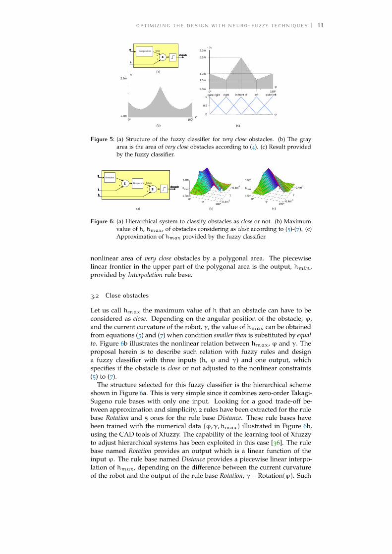
Figure 7: Input-output behavior of the rule base Distance in Figure 6a.
|g|
j h
M M
0.0m
0.4m
2.4m
20.0m 0º
180º
-1
-1
|g| 0.0m -1
0.4m -1
j
2.4m 20.0m
1
0 h
M
M
180º
0º 0 1
j
2.4m 20.0m
1
0 h
M
M
180º
0º 0 1
(a) (c) (b)
Figure 8: (a) Curvature to avoid obstacles according to (9). (b) 25 rules extractedby Wang-Mendel algorithm with a regular 5x5 grid. (c) The 5x5 grid isadjusted to the data by supervised learning.
difference can be understood as the angular position referred to the robotthat the obstacle will have in the future. This is why the antecedents in the5 rules of Distance rule base have been named as quite right, right, in front of,left, and quite left. Their corresponding consequents are: hmax is 1.6m, 2m,4m, 2m, and 1.6m, as shown in Figure 7.
Figure 6c illustrates how the designed fuzzy classifier approximates thenonlinear relation between hmax, ϕ and γ with piecewise linear relations.
3.3 Obstacle avoidance
The minimum magnitude of the curvature to avoid an obstacle is a nonlin-ear function, f, of the closest point of the obstacle (hM and ϕM), as statedin (9). Exploiting the symmetry of the problem, it can be considered thatγ = f(ϕM,hM), when turning to right and γ = f(180 − ϕM,hM), whenturning to left. Figure 8a shows the γ values (when turning to right) ver-sus ϕM and hM. The proposal herein is to approximate such nonlinearrelation with fuzzy rules, that is, to design a fuzzy approximator with twoinputs, hM and ϕM, and one output that specifies the magnitude of thecurvature. In this case, a non-hierarchical system has been selected becauseits complexity is somewhat lower (5 instead of the 9 rules extracted in thehierarchical system) achieving a better approximation. The procedure toobtain the non-hierarchical system follows the techniques described in [37].Firstly, 5 membership functions have been selected as a good initial numberto cover uniformly the universes of discourse of the hM and ϕM variables,as shown in Figure 8b. By using the numerical data (hM,ϕM,γ) shown
optimizing the design with neuro-fuzzy techniques 13
(a) (c) (b)
very far very near near
in
front
of
left
quite
left
right
far medium
j
2.4m 20.0m
1
0 h
M
M
180º
0º 0 1
Rule 1
Rule 2
Rule 3
Rule 4
very far very near near
in
front
of
left
quite
left
right
far medium
j
2.4m 20.0m
1
0 h
M
M
180º
0º 0 1
|g|
j h M
M
0.0m
0.4m
2.4m
20.0m 0º
180º
-1
-1
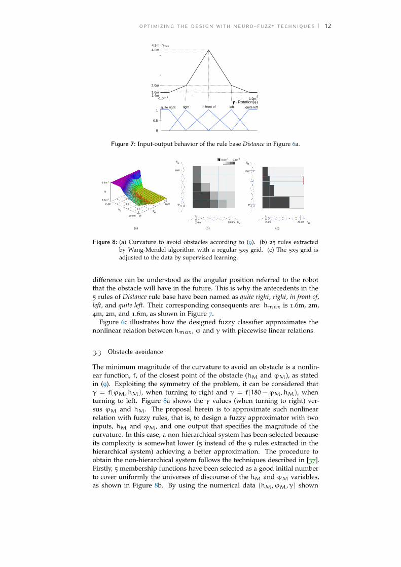
Figure 9: (a) The 25 rules are simplified to 20 rules by merging membership func-tions in ϕM. (b) The 20 rules are simplified to 5 rules by applying FuzzyTabular Simplification method [37]. (c) Approximation of |γ| to avoid ob-stacles provided by the 5-rule fuzzy system.
in Figure 8a and applying Wang-Mendel identification algorithm with theidentification tool of Xfuzzy [37], 25 zero-order Takagi-Sugeno rules (illus-trated as a matrix in Figure 8b) have been obtained. Again the numericaldata (hM,ϕM,γ) have been employed to apply supervised learning to ad-just the membership functions in the antecedents and the singleton valuesin the consequents of these 25 fuzzy rules so as to reduce the approximationerror. The result of such learning is illustrated in Figure 8c. By using thesimplification tool of Xfuzzy, two membership functions covering ϕM canbe merged, as shown in Figure 8c, so that the 25 rules are reduced to 20. Fi-nally, by applying the Fuzzy Tabular Simplification method available in thesimplification tool of Xfuzzy [37], the 20 rules can be reduced to 5 rules, 4 ofthem describing when turning right at maximum and the other concludingno turning for the rest of situations. This is illustrated in Figure 9a and b.The obtained zero-order Takagi-Sugeno system, which decides how muchturning to right (once turning to right has been decided), forces the robot toturn more as more dangerous the obstacle is for the way the robot is goingto take immediately. The closer the obstacle is, the more the robot will turnto right. The fuzzy rules express the following conditions to turn right atmaximum (imagine the robot is going ahead or to its right):
1. If obstacle is very near.
2. If obstacle is near and it is not quite on the left.
3. If obstacle is at medium distance and it is in front of or on the right.
4. If obstacle is far and it is on the right.
In other cases, the robot should keep straight ahead.Since these rules employ fuzzy concepts, the γ values provided by this
system do not switch abruptly but they vary smoothly between maximumturning to right and zero, as shown in Figure 9c.
3.4 Navigation toward the goal
If no obstacles are detected, the robot will turn to right or left or will notturn depending on the difference between the current robot orientation andthe angle α (defined in (11) as a nonlinear function of the robot position, xand y). The approach herein is to use a fuzzy system that approximates thevalue of the robot curvature, as described in [25]. A hierarchical structure
optimizing the design with neuro-fuzzy techniques 14
(a) (b) (c)
-180º
180º
x
a
y
-20m
20m -2m
14m
-180º
180º
x
a
y
-20m
20m -2m
14m Interpolation
x
a
+
-Smoothing
y
Interpolation
x
a
+
-Smoothing
y
Figure 10: (a) Fuzzy system to navigate without obstacles. (b) Angle α according to(10)-(11). (c) Result provided by the fuzzy system.
Table 1: Rules in the rule base Interpolation of Figure 10
IF x is AND y is THEN α is
zero zero 51.3+ 8.2x+ 2.8y
zero near 8.8x
zero far −1.6x
positive-near zero 103.3+ 4.9x+ 7.8y
positive-near near 29.2+ 5.3x− 1.5y
positive-near far −9.4+ 0.3x+ 1.6y
positive-far zero −51.3+ 8.2x− 2.8y
positive-far near −11.2+ 4.1x+ 1.9y
positive-far far 3.7− 0.7x+ 2.8y
with two rule bases connected in cascade, as shown in Figure 10a, has beenselected. The first rule base provides approximately the value of the angle α,depending on the input variables x and y. This module has been adjustedby using numerical data (x,y,α), obtained from (11) and from the followingequation (which achieves continuity for the rest of positions):
α = (x) · arccos(1−
|x|
R
)if (|x|− R)2 + y2 6 R2 (12)
Exploiting the symmetry of the problem, α(x,y) = −α(−x,y), the neuro-fuzzy system has been trained for positive values of x. The best systemfound in terms of approximation error and simplicity is a first-order Takagi-Sugeno system with 9 rules. These rules are shown in Table 1, where thefuzzy sets (zero, near, etc.) in the antecedents are represented by triangularmembership functions similar to those in Figure 5c and Figure 7. Figure 10bshows the values of α versus x and y according to (11) and (12), and Figure10c shows the approximation provided by the rule base Interpolation.
The best option found for the second rule base Smoothing is a zero-orderTakagi-Sugeno system with 2 rules, exploiting symmetry, γ(φ−α) = −γ(α−
φ). These two rules are the following:
1. If (φ−α) is small-positive then γ is 0.4m−1.
2. If (φ−α) is large-positive then γ is 0.07m−1.
results and discussion 15
4 results and discussion
4.1 Simulation and experimental results
The initial and neuro-fuzzy-based controllers have been described with thetool xfedit of Xfuzzy 3, which allows connecting fuzzy and non fuzzy rulebases as well as arithmetic modules.
Simulations have been carried out with the tool xfsim. It simulates thecontroller working in a closed loop with a model of the robot that considersits kinematic and dynamic features. The robot model (which contains themodels of its sensors) provides the new configuration of the robot and thenew information given by the laser. This model is introduced in xfsim as aJava class.
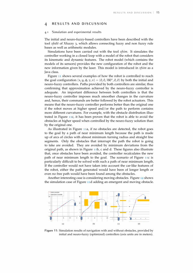
Figure 11 shows several examples of how the robot is controlled to reachthe goal configuration (x,y,φ,γ, v) = (0, 0, 180◦, 0, 0) by both the initial andneuro-fuzzy controllers. Paths provided by both controllers are similar, thusconfirming that approximation achieved by the neuro-fuzzy controller isadequate. An important difference between both controllers is that theneuro-fuzzy controller imposes much smoother changes in the curvatureand, hence, their commands are better followed by the robot actuators. Thismeans that the neuro-fuzzy controller performs better than the original oneif the robot moves at higher speed and/or the path to perform containsmore different curvatures. For example, with the obstacle distribution illus-trated in Figure 11c, it has been proven that the robot is able to avoid theobstacles at higher speed when controlled by the neuro-fuzzy solution thanby the original one.
As illustrated in Figure 11a, if no obstacles are detected, the robot goesto the goal by a path of near minimum length because the path is madeup of arcs of circles with almost minimum turning radius and straight linesegments. Only the obstacles that interrupt the path the robot is goingto take are avoided. They are avoided by minimum deviations from theoriginal path, as shown in Figure 11b, c and d. These figures also illustratethat, once obstacles have been avoided, the controller recalculates the newpath of near minimum length to the goal. The scenario of Figure 11c isparticularly difficult to be solved with such a path of near minimum length.If the controller would not have taken into account the car-like features ofthe robot, either the path generated would have been of longer length oreven no free path would have been found among the obstacles.
Another interesting case is considering moving obstacles. Figure 12 showsthe simulation case of Figure 11d adding an emergent and moving obstacle.
(a)
Initial controller
Optimized Controller
(b) (c) (d)
Figure 11: Simulation results of navigation with and without obstacles, provided byinitial and neuro-fuzzy (optimized) controllers (axis units are in meters).
results and discussion 16
(a) (b) (c)
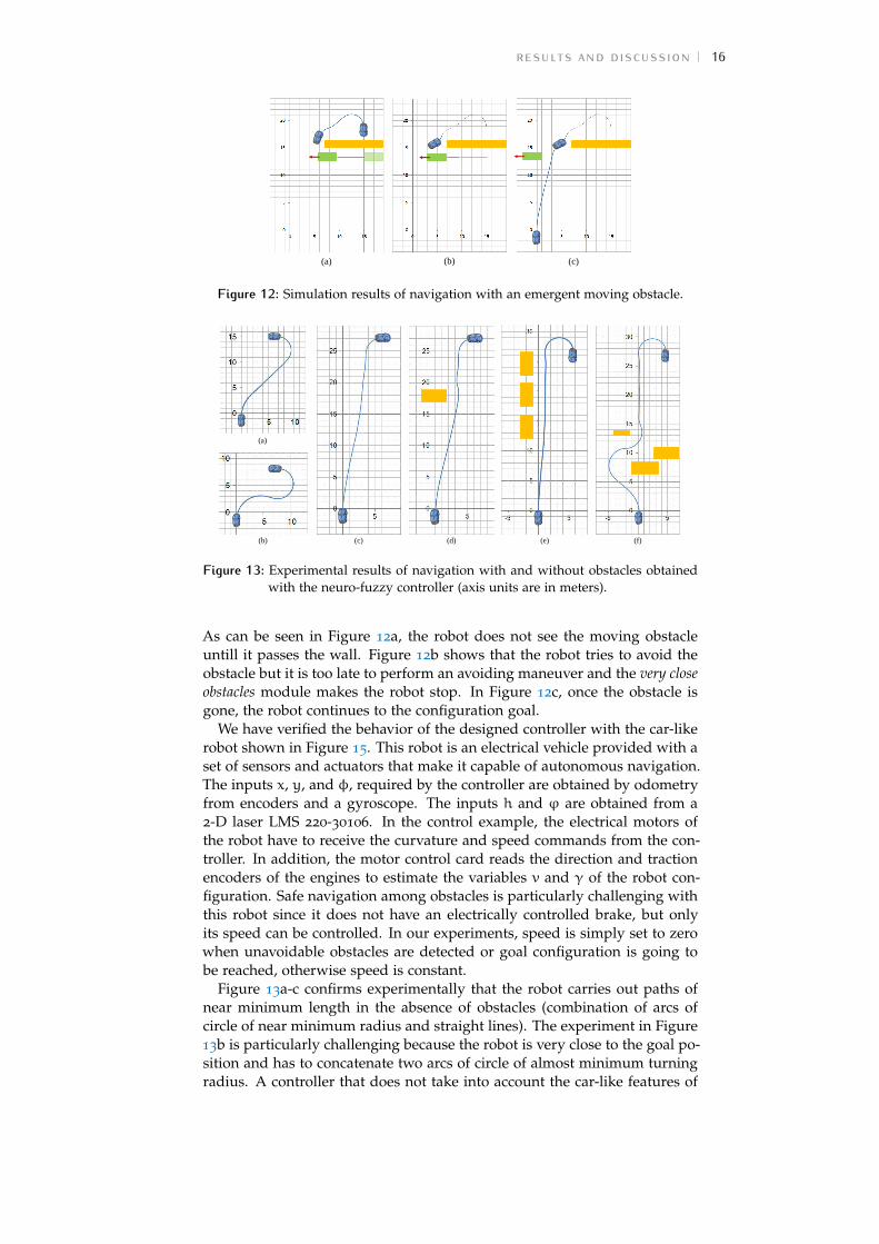
Figure 12: Simulation results of navigation with an emergent moving obstacle.
(a)
(b) (c) (d) (e) (f)
Figure 13: Experimental results of navigation with and without obstacles obtainedwith the neuro-fuzzy controller (axis units are in meters).
As can be seen in Figure 12a, the robot does not see the moving obstacleuntill it passes the wall. Figure 12b shows that the robot tries to avoid theobstacle but it is too late to perform an avoiding maneuver and the very closeobstacles module makes the robot stop. In Figure 12c, once the obstacle isgone, the robot continues to the configuration goal.
We have verified the behavior of the designed controller with the car-likerobot shown in Figure 15. This robot is an electrical vehicle provided with aset of sensors and actuators that make it capable of autonomous navigation.The inputs x, y, and φ, required by the controller are obtained by odometryfrom encoders and a gyroscope. The inputs h and ϕ are obtained from a2-D laser LMS 220-30106. In the control example, the electrical motors ofthe robot have to receive the curvature and speed commands from the con-troller. In addition, the motor control card reads the direction and tractionencoders of the engines to estimate the variables v and γ of the robot con-figuration. Safe navigation among obstacles is particularly challenging withthis robot since it does not have an electrically controlled brake, but onlyits speed can be controlled. In our experiments, speed is simply set to zerowhen unavoidable obstacles are detected or goal configuration is going tobe reached, otherwise speed is constant.
Figure 13a-c confirms experimentally that the robot carries out paths ofnear minimum length in the absence of obstacles (combination of arcs ofcircle of near minimum radius and straight lines). The experiment in Figure13b is particularly challenging because the robot is very close to the goal po-sition and has to concatenate two arcs of circle of almost minimum turningradius. A controller that does not take into account the car-like features of
results and discussion 17
0.4 Ref
0.3
0.2
0.0
0.1
-0.4
-0.3
-0.2
-0.1
-0.5 0 10 20 30 40 50
Real
Curvature (m ) -1
Iteration
Figure 14: Evolution of reference curvature (Ref) provided by the neuro-fuzzy con-troller and actual curvature (Real) of the robot.
(a) (b) (c) (d)
(g)
(e) (f)
(h) (i) (l) (k) (j)
Figure 15: Experimental results of navigation with moving obstacles.
the robot would provide a longer path or even would fail in this scenario.Figure 13d-e shows the minimum deviation from the original path when anobstacle is detected. Such minimum deviation allows the robot navigatingsafely along narrow free spaces, as illustrated in Figure 13f. A success-ful navigation between the obstacles shown in Figure 13f and a successfulconsecution of the goal configuration is very difficult for a controller notoptimized for car-like robots. It is achieved by the neuro-fuzzy controllerbecause it provides a control action that can be tracked by the robot actua-tor. This can be seen in Figure 14, which details a typical evolution of robotcurvature when avoiding an obstacle (this case corresponds to the trajectoryin Figure 13d).
Finally, Figure 15 shows two cases of navigation with moving obstacles.In Figures 15a-f a pedestrian walks toward the path of the robot. As canbe seen, the robot avoids the pedestrian and then it returns to the originalpath. In Figures 15g-l a pedestrian suddenly appears in front of the robot.The very close obstacles module makes the robot stop, avoiding the collision(Figure 15h). Once the pedestrian walks away, the robot returns to the path(Figures 15i-l).
4.2 Implementation results
The initial controller described in Section 2 that applies three navigationfuzzy rules whose symbols are described by equations (1) to (11) has beenexecuted by an embedded system based on MicroBlaze and implementedin a Virtex II-Pro FPGA from Xilinx [38]. MicroBlaze is a 32-bit RISC Har-vard architecture soft processor core with a rich instruction set optimized forembedded applications. In the system designed, MicroBlaze processor in-cludes a floating point unit so as to carry out equations (1) to (11). A timer isadded as peripheral in order to evaluate the number of clock cycles investedby the processor in the four main modules of the control algorithm: evaluat-ing very close obstacles (module 1) and close obstacles (module 2), avoiding

results and discussion 18
Table 2: Number of clock cycles required by the initial and optimized (neuro-fuzzy)embedded controllers
Controller Module 1 Module 2 Module 3 Module 4
Initial (float) 58642 236157 65024 47145
Neuro-fuzzy (float) 2123 5370 4580 21035
Neuro-fuzzy (int) 44 67 141 142
Table 3: Computation time (in seconds) of embedded controllers using 50MHz ofworking frequency
Controller Module 1 Module 2 Module 3 Module 4
Initial (float) 1.17e-3 4.72e-3 1.30e-3 0.94e-3
Neuro-fuzzy (float) 42.46e-6 107.4e-6 91.6e-6 420.7e-6
Neuro-fuzzy (int) 0.88e-6 1.34e-6 2.82e-6 2.84e-6
close obstacles (module 3), and navigating toward the goal (module 4). Theinput variables considered by each module (for example h and ϕ in module1, or ϕ, γ and h in module 2) have been swept considering their universesof discourse (for example ϕ has been swept from 0◦ to 180◦) in order toevaluate the number of clock cycles required by all the possible situations(all possible values at their inputs). The averages of those numbers for eachmodule are shown in the first row of Table 2.
The proposed neuro-fuzzy approach allows a good trade-off betweenmemory resources and computation time. Regarding memory, the parame-ters required to be stored are the partition values of the input universes ofdiscourse and the consequent values, which is a small number since there isa small number of rules (28 rules counting the four modules). This is muchmore efficient than storing in a look-up table the possible control actionsfor all the possible input values. Regarding computation time, the designedneuro-fuzzy controller requires only logical, addition, and multiplicationoperations, while the direct implementation of the equations (1) to (11) (asshown in Section 2) also requires more complex mathematical functions.For any kind of processor, our proposal requires much fewer clock cyclesto compute the control value, especially if the processor has low computa-tional resources. Table 2 supports this affirmation by showing the numberof clock cycles of the same embedded system based on MicroBlaze proces-sor designed for the initial controller. The C code corresponding to the fourmodules required by the neuro-fuzzy controller has been executed on theprocessor using float variables. The second row in Table 2 shows the cy-cles (also the average calculated with all the possible combinations of inputvalues) when the modules are implemented as neuro-fuzzy systems. Thepercentage in clock cycle reduction is higher than 93% in three of the mod-ules. In the Module 4, reduction is inferior (55.4%) mainly because one ofthe rule bases of the neuro-fuzzy solution uses a first-order (instead of azero-order) Takagi-Sugeno inference method.
A further relevant advantage of our proposal is that computation can beperformed with integer variables without a significant lost of precision (Mi-croBlaze works with 32 bits). The third row of Table 2 shows that using in-teger instead of float variables reduces clock cycles in average in two ordersof magnitude (more than 96%). Hence our approach can be implementedefficiently in processors with fixed-point architectures. Table 3 shows a sim-

results and discussion 19
ilar comparison but in terms of computation time, considering a clock cycleof 20ns (50MHz of working frequency).
4.3 Discussion
Previous work on neuro-fuzzy and fuzzy approaches implemented on FP-GAs to control autonomous car-like robots, such as [16], [17] and [19], learnor emulate the expert knowledge of a human driver and focus on parkingproblems (parking without obstacles in [16] and parking in a structured en-vironment in [17]) or focus on path tracking without obstacles [19]. OtherFPGA-based neuro-fuzzy approaches, such as [18], do not take into accountthe constraints of car-like robots. The approach proposed herein is able toprovide paths of smaller length for car-like robots in unstructured environ-ments with obstacles.
Previous work on neuro-fuzzy approaches that learn to provide paths ofsmall length, such as [22], consider structured environments and are lesssuitable for implementation into embedded systems, because they employGaussian membership functions. Others, which are more suitable for em-bedded systems, such as [24] and [25], do not avoid obstacles. The solutionproposed in [25], which is implemented in a Pentium processor working at100MHz, takes about 2ms to compute the reference curvature. The solutionproposed in [24], which is implemented in a DSP (Digital Signal Proces-sor) working at 33MHz, takes about 20 s for a similar computation. In theapproach proposed herein, Module 4, whose task is comparable to the so-lutions in [24] and [25], takes 2.84µs at 50MHz, which means the fastestsolution based on an embedded processor. In addition, the other modulesof the controller designed herein are even faster. This provides the robotwith the capability of performing more complex tasks with the same hard-ware platform or, similarly, allows using platforms with limited resources tocarry out safe navigation. In case that a fast solution is not required by theapplication, the operation frequency can be very low and, hence, a solutionof very low power consumption can be obtained.
The neuro-fuzzy tecnique proposed herein approximates the equations ofa reference controller. Other approximators could have been employed, suchas neural networks based on radial basis functions (RBF NNs). Table 4 com-pares the number of rules and approximation error (expressed as root meansquare error, RMSE) of the four modules designed herein with the numberof neurons in the hidden layer of RBF NNs and their approximation error.The radial basis functions considered have been the product of isosceles tri-angles (to be similar in complexity to the triangular membership functionsand the product connective considered in the neuro-fuzzy approach). TheRBF NNs have been trained with the same numerical data, using also thesupervised learning tool of the Xfuzzy environment. In the case of modules1 and 3, which deal with two inputs, the RBF NNs need 30 and 16 neu-rons, respectively, to obtain the same approximation error, which means anincrease in complexity of approximately 6 and 3.2 times more, respectively.In the case of modules 2 and 4, which deal with three inputs, the curse ofdimensionality, typical of RBF NNs, begins to appear. Although using 150
and 180 neurons (in case of module 2 and 4, respectively), which means anincrease in complexity of approximately 21.4 and 16.4 times, respectively,the approximation errors are worse.
Further research will involve the integration of the designed local con-troller into a hybrid architecture that contains global and other local mod-
conclusions 20
Table 4: Comparison of the neuro-fuzzy proposal with neural networks based onradial basis functions (RBF NNs).
Proposal RBF NNs
Module No. rules RMSE No. hidden neurons RMSE
Module 1 5 0.14 30 0.14
Module 2 7 0.09 150 0.15
Module 3 5 0.07 16 0.07
Module 4 11 0.08 180 0.15
ules so as to cope with complex navigation problems (including drivingbackward) and to deal with the considerable levels of noise present in com-plex robotic systems.
5 conclusionsNeuro-fuzzy techniques have been proven very effective to optimize thedesign of an embedded controller for the free collision navigation of an au-tonomous car-like robot. The control algorithm can be executed rapidly orwith low power consumption by even systems based on fixed-point proces-sors because the rule bases employed contain a few number of rules, thenumber of antecedents is low, and Takagi-Sugeno inference is applied (withantecedents represented by normalized triangular functions). Despite itssimplicity, the controller action is smooth and provides paths of near min-imum length, as has been proven by simulation and experimental results.The methodology to design the neuro-fuzzy controller has been automatedthanks to the CAD tools of the environment Xfuzzy 3, while the FPGA em-bedded system has been developed with the CAD tools from Xilinx.
AcknowledgementsThis work was supported in part by the Spanish Ministerio de Economíay Competitividad under the Project TEC2011-24319 and by Junta de An-dalucía under the Project P09-TEP-4479 (both with support from FEDER).The authors would like to thank the Department of Ingeniería de Sistemas yAutomática, University of Seville, in particular to A. Ollero, J. Ferruz, andF. Leal for advice and collaboration to carry out the experiments with thecar-like robot.
references[1] T.J. Ross, Fuzzy logic with engineering applications, 3rd Edition, Wiley,
2010.
[2] H.-P. Huang, J.-L. Yan and T.-H. Cheng, Development and fuzzy con-trol of a pipe inspection robot, IEEE Transactions on Industrial Elec-tronics 57 (3) (2010) 1088-1095.
[3] P. Rusu, E.M. Petriu, T.E. Whalen, A. Cornell and H.J.W. Spoelder,Behavior-based neuro-fuzzy controller for mobile robot navigation,IEEE Transactions on Instrumentation and Measurement 52 (4) (2003)1335-1340.
References 21
[4] X. Wang and S.X. Yang, A neuro-fuzzy approach to obstacle avoid-ance for a nonholonomic mobile robot, in: Proceedings of the 2003
IEEE/ASME International Conference on Advanced Intelligent Mecha-tronics (AIM’03), 20-24 July 2003, vol. 1, pp. 29-34.
[5] K. Basterretxea and I. del Campo, Electronic hardware for fuzzy com-putation. In A. Laurent and M-J. Lesot (Eds.), Scalable fuzzy algorithmsfor data management and analysis: Methods and design, pp. 1-30, IGIGlobal, 2010.
[6] A. Malinowski and H. Yu, Comparison of embedded system design forindustrial applications, IEEE Transactions on Industrial Informatics 7
(2) (2011) 244-254.
[7] E. Monmasson, L. Idkhajine, M.N. Cirstea, I. Bahri, A. Tisan and M.W.Naouar, FPGAs in industrial control applications, IEEE Transactions onIndustrial Informatics 7 (2) (2011) 224-243.
[8] J.J. Rodriguez-Andina, M.J. Moure and M.D. Valdes, Features, Designtools and application domains of FPGAs, IEEE Transactions on Indus-trial Electronics 54 (4) (2007) 1810-1823.
[9] D. Majoe, L. Widmer, L. Ling, J. Kao and J. Gutknecht, A reconfigurablemulti-core computing platform for robotics and e-Health applications,in: Proceedings of the 2012 IEEE/ACIS 11th International Conferenceon Computer and Information Science (ICIS’12), 30 May - 1 June 2012,pp. 451-456.
[10] M.A. Cavuslu, C. Karakuzu and F. Karakaya, Neural identification ofdynamic systems on FPGA with improved PSO learning, Applied SoftComputing 12 (9) (2012) 2707-2718.
[11] C.-Y. Chen, R.-C. Hwang and Y.-J. Chen, A passive auto-focus cameracontrol system, Applied Soft Computing 10 (1) (2010) 296-303.
[12] P. Brox, I. Baturone and S. Sánchez-Solano, Fuzzy logic-based embed-ded system for video de-interlacing, Applied Soft Computing 14 (C)(2014) 338-346.
[13] F. Montesino-Pouzols, A. Barriga-Barros, D.R. López and S. Sánchez-Solano, Enabling fuzzy technologies in high performance networkingvia an open FPGA-based development platform, Applied Soft Comput-ing 12 (4) (2012) 1440-1450.
[14] S. Sánchez-Solano, M. Brox, E. del Toro, P. Brox and I. Baturone, Model-based design methodology for rapid development of fuzzy controllerson FPGAs, IEEE Transactions on Industrial Informatics 9 (3) (2013)1361-1370.
[15] R. Sepúlveda, O. Montiel, O. Castillo and P. Melin, Embedding a highspeed interval type-2 fuzzy controller for a real plant into an FPGA,Applied Soft Computing 12 (3) (2012) 988-998.
[16] S. Sánchez-Solano, A.J. Cabrera, I. Baturone, F.J. Moreno-Velo and M.Brox, FPGA implementation of embedded fuzzy controllers for roboticapplications, IEEE Transactions on Industrial Electronics 54 (4) (2007)1937-1945.
References 22
[17] T.S. Li, S.-J. Chang and Y.-X. Chen, Implementation of human-like driv-ing skills by autonomous fuzzy behavior control on an FPGA-basedcar-like mobile robot, IEEE Transactions on Industrial Electronics 50 (5)(2003) 867-880.
[18] M.N. Mahyuddin, C.Z. Wei and M.R. Arshad, Neuro-fuzzy algorithmimplemented in Altera’s FPGA for mobile robot’s obstacle avoidancemission, in: Proceedings of the 2009 IEEE Region 10 Conference (TEN-CON’09), 23-26 January 2009, pp. 1-6.
[19] S.G. Tzafestas, K.M. Deliparaschos and G.P. Moustris, Fuzzy logic pathtracking control for autonomous non-holonomic mobile robots: Designof System on a Chip, Robotics and Autonomous Systems 58 (8) (2010)1017-1027.
[20] J. Ferruz, V.M. Vega, A. Ollero and V. Blanco, Reconfigurable control ar-chitecture for distributed systems in the HERO autonomous helicopter,IEEE Transactions on Industrial Electronics 58 (12) (2011) 5311-5318.
[21] T. Takagi and M. Sugeno, Fuzzy identification of systems and its appli-cations to modeling and control, IEEE Transactions on Systems, Man,and Cybernetics 15 (1) (1985) 116-132.
[22] K. Demirli and M. Khoshnejad, Autonomous parallel parking of a car-like mobile robot by a neuro-fuzzy sensor-based controller, Fuzzy Setsand Systems 160 (19) (2009) 2876-2891.
[23] N. Uchiyama, T. Hashimo, S. Sano and S. Takagi, Model-reference con-trol approach to obstacle avoidance for a human-operated mobile robot,IEEE Transactions on Industrial Electronics 56 (10) (2009) 3892-3896.
[24] I. Baturone, F.J. Moreno-Velo, V. Blanco and J. Ferruz, Design of embed-ded DSP-based fuzzy controllers for autonomous mobile robots, IEEETransactions on Industrial Electronics 55 (2) (2008) 928-936.
[25] I. Baturone, F.J. Moreno-Velo, S. Sánchez-Solano and A. Ollero, Auto-matic design of fuzzy controllers for car-like autonomous robots, IEEETransactions on Fuzzy Systems 12 (4) (2004) 447-465.
[26] K. Samsudin, F.A. Ahmad and S. Mashohor, A highly interpretablefuzzy rule base using ordinal structure for obstacle avoidance of mobilerobot, Applied Soft Computing 11 (2) (2011) 1631-1637.
[27] Xfuzzy: Fuzzy logic design tools. Available at: http://www.imse-cnm.
csic.es/Xfuzzy
[28] J.C. Latombe, Robot motion planning, Kluwer Academic Publishers,1991.
[29] R.A. Brooks, A robust layered control system for a mobile robot, IEEEJournal on Robotics and Automation 2 (1) (1986) 14-23.
[30] M.J. Wooldridge, An introduction to multiagent systems, John Wiley &Sons Ltd., 2009.
[31] L.E. Dubins, On curves of minimal length with a constraint on aver-age curvature and with prescribed initial and terminal positions andtangents, American Journal of Mathematics 79 (3) (1957) 497-516.
References 23
[32] J.A. Reeds and R.A. Shepp, Optimal path for a car that goes both for-ward and backward, Pacific Journal of Mathematics 145 (2) (1990) 367-393.
[33] G. Desaulniers, On shortest paths for a car-like robot maneuveringaround obstacles, Robotics and Autonomous Systems 17 (3) (1996) 139-148.
[34] N. Ghita and M. Kloetzer, Trajectory planning for a car-like robot by en-vironment abstraction, Robotics and Autonomous Systems 60 (4) (2012)609-619.
[35] R. Battiti, First- and second-order methods for learning: between steep-est descent and Newton’s method, Neural Computation 4 (2) (1992)141-166.
[36] F.J. Moreno-Velo, I. Baturone, A. Barriga and S. Sánchez-Solano, Auto-matic tuning of complex fuzzy systems with Xfuzzy, Fuzzy Sets andSystems 158 (18) (2007) 2026-2038.
[37] I. Baturone, F.J. Moreno-Velo and A. Gersnoviez, A CAD approach tosimplify fuzzy system description, in: Proceedings of the 2006 IEEEInternational Conference on Fuzzy Systems (FUZZ-IEEE’06), 16-21 July2006, pp. 2392-2399.
[38] Virtex-II Pro and Virtex-II Pro X FPGA user guide, Xilinx, 2007.