New Insights into Disinfection Byproduct Formation and

University of Arkansas, FayettevilleScholarWorks@UARK

Theses and Dissertations

8-2012

New Insights into Disinfection ByproductFormation and Control: Assessing DissolvedOrganic Matter Diffusivity and ChemicalFunctionalityAshley PiferUniversity of Arkansas, Fayetteville

Follow this and additional works at: http://scholarworks.uark.edu/etd

Part of the Civil Engineering Commons, and the Environmental Engineering Commons

This Dissertation is brought to you for free and open access by ScholarWorks@UARK. It has been accepted for inclusion in Theses and Dissertations byan authorized administrator of ScholarWorks@UARK. For more information, please contact [email protected], [email protected].

Recommended CitationPifer, Ashley, "New Insights into Disinfection Byproduct Formation and Control: Assessing Dissolved Organic Matter Diffusivity andChemical Functionality" (2012). Theses and Dissertations. 498.http://scholarworks.uark.edu/etd/498

http://scholarworks.uark.edu?utm_source=scholarworks.uark.edu%2Fetd%2F498&utm_medium=PDF&utm_campaign=PDFCoverPages

http://scholarworks.uark.edu/etd?utm_source=scholarworks.uark.edu%2Fetd%2F498&utm_medium=PDF&utm_campaign=PDFCoverPages

http://scholarworks.uark.edu/etd?utm_source=scholarworks.uark.edu%2Fetd%2F498&utm_medium=PDF&utm_campaign=PDFCoverPages

http://network.bepress.com/hgg/discipline/252?utm_source=scholarworks.uark.edu%2Fetd%2F498&utm_medium=PDF&utm_campaign=PDFCoverPages

http://network.bepress.com/hgg/discipline/254?utm_source=scholarworks.uark.edu%2Fetd%2F498&utm_medium=PDF&utm_campaign=PDFCoverPages

http://scholarworks.uark.edu/etd/498?utm_source=scholarworks.uark.edu%2Fetd%2F498&utm_medium=PDF&utm_campaign=PDFCoverPages

mailto:[email protected],%[email protected]

NEW INSIGHTS INTO DISINFECTION BYPRODUCT FORMATION AND CONTROL: ASSESSING DISSOLVED ORGANIC MATTER DIFFUSIVITY AND CHEMICAL

FUNCTIONALITY

NEW INSIGHTS INTO DISINFECTION BYPRODUCT FORMATION AND CONTROL: ASSESSING DISSOLVED ORGANIC MATTER DIFFUSIVITY AND CHEMICAL

FUNCTIONALITY

A dissertation submitted in partial fulfillment of the requirements for the degree of

Doctor of Philosophy in Civil Engineering

By

Ashley Dale Pifer University of Arkansas

Bachelor of Science in Civil Engineering, 2009

August 2012 University of Arkansas

ABSTRACT

Methods were developed for application of asymmetric flow field-flow fractionation

(AF4) and fluorescence parallel factor (PARAFAC) analysis to raw and treated samples from

drinking water sources to improve characterizations of dissolved organic matter (DOM) and

discover DOM properties correlated to disinfection byproduct (DBP) formation potential (FP).

Raw water samples were collected from a reservoir, adjusted to pH 6, 7, and 8 and subjected to

(1) jar tests using aluminum sulfate (alum) and (2) treatment with magnetic ion exchange

(MIEX®) resin. Both treatments were followed by DBPFP tests at pH 7. AF4 was used to size

DOM in raw and alum treated samples at pH 6 and 8. AF4 fractograms showed that DOM

removal was more effective at pH 6 than at pH 8, and preferential removal of larger-sized DOM

occurred at pH 6 but not at pH 8.

A fluorescence-PARAFAC model was constructed using excitation-emission matrices

(EEMs) from all samples. A strong linear correlation (r2 = 0.87) between chloroform FP and a

humic-like PARAFAC component (C1) was developed. This correlation was a significant

improvement over the correlation (r2 = 0.03) between chloroform FP and specific ultraviolet

absorbance at 254 nm (SUVA254), a DBPFP surrogate commonly used in drinking water

treatment plants to optimize DOM removal processes. This indicated that chloroform FP-C1

correlations were not treatment-specific.

Alum coagulation at pH 6, 7, and 8 and DBPFP tests at pH 7 were performed on a set of

raw waters from eleven drinking water treatment plants from across the United States. AF4 was

used to size DOM before and after alum coagulation, and showed similar results to the earlier

study, i.e., increased removal at pH 6 compared to pH 8. A fluorescence-PARAFAC model was

constructed and total trihalomethane (TTHM) FP was strongly correlated (r2 = 0.91) to C1 for

eight water sources. TTHMFP-SUVA254 correlations for ten locations were weak (r2 = 0.15),

which indicated that C1 was an improved DBPFP surrogate relative to SUVA254 and could be

used as a surrogate to select and optimize DBP precursor removal processes.

This dissertation is approved for recommendation to the Graduate Council. Dissertation Director: _______________________________________ Dr. Julian L. Fairey Dissertation Committee: _______________________________________ Dr. Jamie A. Hestekin _______________________________________ Dr. David M. Miller _______________________________________ Dr. Rodney D. Williams

DISSERTATION DUPLICATION RELEASE I hereby authorize the University of Arkansas Libraries to duplicate this dissertation when needed for research and/or scholarship. Agreed _______________________________________ Ashley Pifer Refused _______________________________________ Ashley Pifer

ACKNOWLEDGMENTS

I would like to thank my family and friends for the encouragement, support, and comic

relief. I would like to thank my advisor and committee members for their guidance. I am grateful

to the University of Arkansas for the Distinguished Academic Fellowship.

TABLE OF CONTENTS

Chapter 1: Introduction ....................................................................................................................1

Problem Statement ...............................................................................................................2

Objectives and Approach .....................................................................................................3

Document Organization .......................................................................................................5

References ............................................................................................................................5

Chapter 2: Coupling Asymmetric Flow-Field Flow Fractionation and Fluorescence Parallel

Factor Analysis Reveals Stratification of Dissolved Organic Matter in a Drinking Water

Reservoir ....................................................................................................................................8

1. Introduction ....................................................................................................................10

2. Materials and Methods...................................................................................................14

2.1. Site Description...............................................................................................14

2.2. Sample Handling and Collection ....................................................................15

2.3. Water Quality Tests ........................................................................................15

2.4. Asymmetric Flow-Field Flow Fractionation ..................................................17

2.5. Fluorescence ...................................................................................................19

3. Calculation .....................................................................................................................22

4. Results and Discussion ..................................................................................................23

4.1. Water Quality Parameters ................................................................................23

4.2. AF4-Fractograms .............................................................................................24

4.3. Fluorescence-PARAFAC Analyses .................................................................27

5. Conclusions ....................................................................................................................29

6. References ......................................................................................................................39

Appendix 1 Supporting Material for “Coupling Asymmetric Flow-Field Flow Fractionation and

Fluorescence Parallel Factor Analysis Reveals Stratification of Dissolved Organic Matter in a

Drinking Water Reservoir” ......................................................................................................44

Chapter 3 Improving on SUVA254 Using Fluorescence-PARAFAC Analysis and Asymmetric

Flow-Field Flow Fractionation for Assessing Disinfection Byproduct Formation and Control53

1. Introduction and Motivation ..........................................................................................55


2.1. Site description ...............................................................................................59

2.2. Sample collection and handling ......................................................................59


2.4. Jar Tests ..........................................................................................................60

2.5. Disinfection byproducts ..................................................................................61

2.6. Asymmetric flow-field flow fractionation ......................................................62

2.7. Fluorescence-PARAFAC analysis ..................................................................62


3.1. Raw Water Parameters....................................................................................63

3.2. AF4-UV254 Fractograms .................................................................................63

3.3. Fluorescence-PARAFAC Analysis.................................................................65

3.4. Disinfection Byproducts .................................................................................66

3.5. Correlations between DBP formation and DOM properties ...........................68

4. Conclusions ....................................................................................................................69

5. References ......................................................................................................................78

Appendix 2 Supplementary Data for Improving on SUVA254 Using Fluorescence-PARAFAC

Analysis and Asymmetric Flow-Field Flow Fractionation for Assessing Disinfection

Byproduct Formation and Control ...........................................................................................81


1.1. Sample collection and handling. .....................................................................82

1.2. Water Quality Tests. .......................................................................................82

1.3. Fluorescence-PARAFAC analysis. .................................................................82


2.1. Raw Water Parameters....................................................................................83

2.2. References .......................................................................................................90

Chapter 4 Tracking Disinfection Byproduct Precursor Removal by Magnetic Ion Exchange Resin

and Alum Coagulation Using Fluorescence-PARAFAC .........................................................91

1. Introduction and Motivation ..........................................................................................93


2.1. Sampling Locations ........................................................................................97


2.3. MIEX® Experiments .......................................................................................98

2.4. Disinfection Byproduct Formation Potential Tests ........................................98

2.5. Fluorescence-PARAFAC Analysis.................................................................99

3. Results and Discussion ................................................................................................100

3.1. Raw Water Parameters..................................................................................100

3.2. Fluorescence-PARAFAC Analysis...............................................................100

3.3. Specific Ultraviolet Absorbance ...................................................................103

3.4. Disinfection Byproduct Formation Potential ................................................103

3.5. Correlations Between DBPs and DBP-Precursor Properties ........................104

4. Conclusions ..................................................................................................................105

5. References ....................................................................................................................114

Chapter 5 Assessing Fluorescence-PARAFAC as a Disinfection Byproduct Formation Potential

Surrogate in Drinking Water Sources from Diverse Watersheds ..........................................117

1. Introduction ..................................................................................................................118

2. Experimental ................................................................................................................120

2.1. Sample collection and handling. ...................................................................120

2.2. Glassware and reagents. ................................................................................121

2.3. Water quality tests. .......................................................................................122

2.4. Jar tests. .........................................................................................................122

2.5. Disinfection byproducts. ...............................................................................122

2.6. Asymmetric flow-field flow fractionation. ...................................................123

2.7. Fluorescence-PARAFAC analysis. ...............................................................123

3. Results and Discussion ................................................................................................124

3.1. Raw water parameters. ..................................................................................124

3.2. Size characterization of chromophoric dissolved organic matter. ................125

3.3. Fluorescence-PARAFAC Analysis...............................................................126

3.4. Disinfection Byproducts. ..............................................................................128

3.5. Correlations between TTHMFP and DOM properties. ................................129

4. Associated Content ......................................................................................................131

5. Author Information ......................................................................................................131

6. References ....................................................................................................................140

Appendix 3 Supporting Information for Assessing Fluorescence-PARAFAC for Prediction of

Disinfection Byproduct Formation Potential in Drinking Water from Diverse Watersheds .143

Chapter 6: Conclusion..................................................................................................................150

1. Summary ......................................................................................................................151

1.1. Objective 1 – Development of AF4 and fluorescence-PARAFAC methods 152

1.2. Objective 2 – Impact of treatment on DOM properties ................................152

1.3. Objective 3 – DBPFP-PARAFAC correlations for alum-treated waters ......154

1.4. Objective 4 – Validation of DBPFP-PARAFAC correlations for two DOM

removal processes .........................................................................................154

1.5. Objective 5 – Validation of DBPFP-PARAFAC correlations for eleven

source waters ................................................................................................154

2. Significance and future work .......................................................................................155

LIST OF PAPERS

CHAPTER 2

Pifer, A. D., Miskin, D. R., Cousins, S. L. and Fairey, J. L., 2011. Coupling asymmetric flow-field flow fractionation and fluorescence parallel factor analysis reveals stratification of dissolved organic matter in a drinking water reservoir. Journal of Chromatography A 1218 (27), 4167-4178.

CHAPTER 3

Pifer, A. D. and Fairey, J. L., 2012. Improving on SUVA254 using fluorescence-PARAFAC analysis and asymmetric flow-field flow fractionation for assessing disinfection byproduct formation and control. Water Research 46 (9), 2927-2936.

CHAPTER 4

Pifer, A. D., Cousins, S. L. and Fairey, J. L., submitted. Tracking disinfection byproduct precursor removal by magnetic ion exchange resin and alum coagulation using fluorescence-PARAFAC, University of Arkansas.

CHAPTER 5

Pifer, A. D. and Fairey, J. L., submitted. Assessing fluorescence-PARAFAC as a disinfection byproduct formation potential surrogate in drinking water sources from diverse watersheds, University of Arkansas.

1

CHAPTER 1

Introduction

2

1. PROBLEM STATEMENT

Disinfection of drinking water has been crucial in the protection of public health since the

early twentieth century, but is not without challenges. In the 1970s, Rook reported the formation

of haloforms following chlorination of natural waters (Rook 1976; 1977) from reactions with

dissolved organic matter (DOM), which is ubiquitous in surface- and ground waters.

Trihalomethanes (THMs) are the most abundant group of DBPs formed during chlorination, and

have been linked to increased health risks (Cantor et al. 1998; Nieuwenhuijsen et al. 2000). The

sum of the four THMs were regulated in drinking water under the United States Environmental

Protection Agency’s (USEPA) Stage 1 Disinfectants/Disinfection Byproducts (D/DBP) rule;

THM regulations became more stringent in the promulgation of the Stage 2 D/DBP rule.

Drinking water treatment plant (DWTP) managers can draw from a two-pronged approach to

decrease formation of THMs and achieve regulatory compliance: (1) alter the disinfectant and/or

(2) remove more DOM (e.g., by processes such as enhanced coagulation, ion exchange). A 1997

survey of 100 DWTPs showed that 20 exceeded the USEPA’s maximum contaminant level

(MCL) for total THMs of 80 µg/L (Arora et al. 1997). This is due in part to the complexity and

variability of DBP precursors within the DOM pool and the limited metrics (e.g. specific

ultraviolet absorbance at 254 nm (SUVA254) and total organic carbon (TOC)) that are used to

design DBP precursor removal processes. Development of highly effective DOM removal

strategies would be aided by improved DOM characterization methods and an increase in

understanding of DOM properties before and after treatment.

DOM has been physically and chemically characterized by a variety of techniques (Kitis

et al. 2002; Yohannes et al. 2005; Cawley et al. 2009; Worms et al. 2010) which have led to

valuable insights into DBP formation (Kim and Yu 2005; Yang et al. 2008; Chu et al. 2010).

3

However, many techniques require large sample volumes, pre-concentration, and perturbations

in acid/base chemistry, which can make characterizations of samples treated at the laboratory

scale difficult and can even introduce artifacts (Gadmar et al. 2005). Symmetrical flow field-flow

fractionation (FlFFF) and asymmetrical FlFFF (AF4) have been used to separate and size DOM

in natural water samples (Floge and Wells 2007; Alasonati et al. 2010) without need for pre-

concentration, interaction with a stationary phase, or perturbations of solution chemistry.

Although these relatively recent techniques have many advantages (Schimpf and Wahlund 1997;

Yohannes et al. 2005), FlFFF and AF4 are not yet commonly applied to drinking water treatment

studies.

Fluorescence spectroscopy is becoming a common tool for chemical DOM

characterizations (Coble et al. 1990; Coble 1996; Hall et al. 2005; Korshin et al. 2007) and has

been applied to DBP studies (Roccaro et al. 2009). The use of parallel factor analysis

(PARAFAC), a statistical algorithm used to decompose fluorescence excitation emission

matrices into fluorophores (called components) (Andersen and Bro 2003), has simplified

identification of relationships between DBPFP and components. Strong DBPFP-PARAFAC

correlations have been reported within a DWTP (Johnstone et al. 2009), but these correlations

have not been verified for different treatment processes or a wide range of source waters.

Although fluorescence-PARAFAC measures bulk DOM properties, it has the potential to

be a useful DBPFP surrogate for DWTPs.

2. OBJECTIVES AND APPROACH

The overall objective of this work was to relate physicochemical DOM characteristics to

DBP formation and control, which could help DWTPs curb DBPs. The characterization

techniques used in this work were chosen such that sample preparation and perturbation were

4

minimized to better represent DOM behavior within DWTPs. Throughout this work, continuous

DOM size distributions were obtained using AF4 coupled with absorbance at 254 nm (UV254).

AF4-UV254 data in the form of fractograms allowed assessment of spatial and temporal DOM

variability and visualization of preferential removal of specific DOM sizes by DOM removal

processes. Fluorescence-PARAFAC analysis data were used to identify correlations between

chemical DOM characteristics and DBP formation before and after simulated drinking water

treatment processes, and the broad applicability of these correlations was investigated. Specific

objectives were to:

(1) Develop detailed methods for AF4-UV254 and fluorescence-PARAFAC for analysis of

DOM in natural water samples.

(2) Investigate the impacts of DOM removal processes on physicochemical DOM

properties.

(3) Develop correlations between formation potential (FP) of individual DBPs and

fluorescence-PARFAC components using samples collected from the four drinking water

treatment plants on Beaver Lake before and after alum coagulation.

(4) Investigate the applicability of DBPFP-PARAFAC correlations to waters treated with

magnetic ion exchange (MIEX) resin.

(5) Assess the broad applicability of DBPFP-PARAFAC correlations using raw water

samples collected from drinking water treatment plants across the United States.

The correlations discovered in this work could be used by drinking water treatment plants

to not only predict DBP formation, but also to select and optimize DOM removal strategies with

greater success than is possible using traditional bulk metrics such as SUVA254.

5

3. DOCUMENT ORGANIZATION

This dissertation comprises two published and two submitted journal article which build

on each other to address the specific research objectives. Chapter 1 contains the problem

statement, general research objectives, and approaches used for this work. Chapter 2 is a

published article and its supplementary data (Appendix 1) regarding objective (1). Chapter 3 is a

published article and its supplementary data (Appendix 2) which address objectives (2) and (3).

Chapter 4 is a submitted paper on objectives (2) and (4). Chapter 5 is a submitted paper and its

supplementary data (Appendix 3) which focus on objectives (2) and (5). Chapter 6 contains

overall conclusions, contributions to the field of drinking water treatment, and recommendations

for future studies.

4. REFERENCES

Alasonati, E., Slaveykova, V. I., Gallard, H., Croue, J. P. and Benedetti, M. F., 2010. Characterization of the colloidal organic matter from the Amazonian basin by asymmetrical flow field-flow fractionation and size exclusion chromatography. Water Research 44 (1), 223-231.

Andersen, C. M. and Bro, R., 2003. Practical aspects of PARAFAC modeling of fluorescence excitation-emission data. Journal of Chemometrics 17 (4), 200-215.

Arora, H., LeChevallier, M. W. and Dixon, K. L., 1997. DBP occurrence survey. Journal American Water Works Association 89 (6), 60-68.

Cantor, K. P., Lynch, C. F., Hildesheim, M. E., Dosemeci, M., Lubin, J., Alavanja, M. and Craun, G., 1998. Drinking water source and chlorination byproducts I. Risk of bladder cancer. Epidemiology 9 (1), 21-28.

Cawley, K. M., Hakala, J. A. and Chin, Y. P., 2009. Evaluating the triplet state photoreactivity of dissolved organic matter isolated by chromatography and ultrafiltration using an alkylphenol probe molecule. Limnology and Oceanography-Methods 7, 391-398.

Chu, W.-H., Gao, N.-Y., Deng, Y. and Krasner, S. W., 2010. Precursors of Dichloroacetamide, an Emerging Nitrogenous DBP Formed during Chlorination or Chloramination. Environmental Science & Technology 44 (10), 3908-3912.

Coble, P. G., 1996. Characterization of marine and terrestrial DOM in seawater using excitation emission matrix spectroscopy. Marine Chemistry 51 (4), 325-346.

6

Coble, P. G., Green, S. A., Blough, N. V. and Gagosian, R. B., 1990. Characterization of dissolved organic matter in the Black Sea by fluorescence spectroscopy. Nature 348 (6300), 432-435.

Floge, S. A. and Wells, M. L., 2007. Variation in colloidal chromophoric dissolved organic matter in the Damariscotta Estuary, Maine. Limnology and Oceanography 52 (1), 32-45.

Gadmar, T. C., Vogt, R. D. and Evje, L., 2005. Artifacts in XAD-8 NOM fractionation. International Journal of Environmental Analytical Chemistry 85 (6), 365-376.

Hall, G. J., Clow, K. E. and Kenny, J. E., 2005. Estuarial Fingerprinting through Multidimensional Fluorescence and Multivariate Analysis. Environmental Science & Technology 39 (19), 7560-7567.

Johnstone, D. W., Sanchez, N. P. and Miller, C. M., 2009. Parallel Factor Analysis of Excitation-Emission Matrices to Assess Drinking Water Disinfection Byproduct Formation During a Peak Formation Period. Environmental Engineering Science 26 (10), 1551-1559.

Kim, H. C. and Yu, M. J., 2005. Characterization of natural organic matter in conventional water treatment processes for selection of treatment processes focused on DBPs control. Water Research 39 (19), 4779-4789.

Kitis, M., Karanfil, T., Wigton, A. and Kilduff, J. E., 2002. Probing reactivity of dissolved organic matter for disinfection by-product formation using XAD-8 resin adsorption and ultrafiltration fractionation. Water Research 36 (15), 3834-3848.

Korshin, G. V., Benjamin, M. M., Chang, H. S. and Gallard, H., 2007. Examination of NOM chlorination reactions by conventional and stop-flow differential absorbance spectroscopy. Environmental Science & Technology 41 (8), 2776-2781.

Nieuwenhuijsen, M. J., Toledano, M. B., Eaton, N. E., Fawell, J. and Elliott, P., 2000. Chlorination disinfection byproducts in water and their association with adverse reproductive outcomes: a review. Occupational and Environmental Medicine 57 (2), 73-85.

Roccaro, P., Vagliasindi, F. G. A. and Korshin, G. V., 2009. Changes in NOM Fluorescence Caused by Chlorination and their Associations with Disinfection by-Products Formation. Environmental Science & Technology 43 (3), 724-729.

Rook, J. J., 1976. Haloforms in drinking water. Journal American Water Works Association 68 (3), 168-172.

Rook, J. J., 1977. Chlorination reactions of fulvic acids in natural waters. Environmental Science & Technology 11 (5), 478-482.

Schimpf, M. E. and Wahlund, K. G., 1997. Asymmetrical flow field-flow fractionation as a method to study the behavior of humic acids in solution. Journal of Microcolumn Separations 9 (7), 535-543.

7

Worms, I. A. M., Al-Gorani Szigeti, Z., Dubascoux, S., Lespes, G., Traber, J., Sigg, L. and Slaveykova, V. I., 2010. Colloidal organic matter from wastewater treatment plant effluents: Characterization and role in metal distribution. Water Research 44 (1), 340-350.

Yang, X., Shang, C., Lee, W., Westerhoff, P. and Fan, C., 2008. Correlations between organic matter properties and DBP formation during chloramination. Water Research 42 (8-9), 2329-2339.

Yohannes, G., Wiedmer, S. K., Jussila, M. and Riekkola, M. L., 2005. Fractionation of Humic Substances by Asymmetrical Flow Field-Flow Fractionation. Chromatographia 61 (7), 359-364.

8

CHAPTER 2

Coupling Asymmetric Flow-Field Flow Fractionation and Fluorescence Parallel Factor

Analysis Reveals Stratification of Dissolved Organic Matter in a Drinking Water Reservoir

9

ABSTRACT

Using asymmetrical flow field-flow fractionation (AF4) and fluorescence parallel factor analysis

(PARAFAC), we showed physicochemical properties of chromophoric dissolved organic matter

(CDOM) in the Beaver Lake Reservoir (Lowell, AR) were stratified by depth. Sampling was

performed at a drinking water intake structure from May-July, 2010 at three depths (3-, 10-, and

18-m) below the water surface. AF4-fractograms showed that the CDOM had diffusion

coefficient peak maximums between 3.5- and 2.8×10-6 cm2 s-1, which corresponded to a

molecular weight range of 680-1,950 Da and a size of 1.6-2.5 nm. Fluorescence excitation-

emission matrices of whole water samples and AF4-generated fractions were decomposed with a

PARAFAC model into five principal components. For the whole water samples, the average total

maximum fluorescence was highest for the 10-m depth samples and lowest (about 40% less) for

18-m depth samples. While humic-like fluorophores comprised the majority of the total

fluorescence at each depth, a protein-like fluorophore was in the least abundance at the 10-m

depth, indicating stratification of both total fluorescence and the type of fluorophores. The results

present a powerful approach to investigate CDOM properties and can be extended to investigate

CDOM reactivity, with particular applications in areas such as disinfection byproduct formation

and control and evaluating changes in drinking water source quality driven by climate change.

KEYWORDS

Diffusion coefficient, polystyrene sulfonate salt, PARAFAC, dissolved organic matter

stratification, disinfection byproduct precursors

10

1. INTRODUCTION

In aqueous systems, the term dissolved organic matter (DOM) is used to refer to mixtures

of molecules comprised mainly of organic carbon, present in ground and surface waters at low

milligram as carbon per liter (mg C L-1) levels. DOM controls geochemical processes, affecting

transport, speciation, and bioavailability of trace elements (Santschi et al. 2002), serves as a

carbon substrate for the growth of biofilms in water distribution systems (LeChevallier et al.

1996), and reacts with drinking water disinfectants to form disinfection byproducts, DBPs (Rook

1977). The formation of DBPs in treated drinking waters is a public health issue, as many DBPs

are regulated because they are suspected human carcinogens. Aquatic DOM is derived from

terrestrial and aquatic sources, and can undergo biotic (e.g., microbial) and abiotic (e.g.,

photolysis) transformations, and, as such, exists as a dynamic carbon pool, the properties of

which can vary temporally and spatially (Huguet et al. 2009). Because of its importance in

aquatic systems, detailed DOM characterization techniques are needed to understand its fate in

the environment and to develop strategies to minimize its deleterious effects in engineered

treatment processes.

Because of the physical and chemical diversity that exists within the aquatic DOM pool,

researchers have attempted to isolate various DOM fractions of like size and/or similar chemical

composition. Commonly used physicochemical separations include resin adsorption techniques

(Kitis et al. 2002; Chu et al. 2010), liquid chromatography (Worms et al. 2010), alum

coagulation and activated carbon adsorption (Kitis 2001), ultrafiltration (Kitis et al. 2002;

Cawley et al. 2009), and flow field-flow fractionation (FlFFF) (Yohannes et al. 2005; Baalousha

and Lead 2007; Floge and Wells 2007; Dubascoux et al. 2008). Once a given DOM fraction has

been separated, various analytical techniques are often applied with improved resolution, such as

11

ultraviolet (UV) spectroscopy (Alasonati et al. 2010; Stolpe et al. 2010; Worms et al. 2010),

measurement of dissolved organic carbon (DOC) (Reszat and Hendry 2005), inductively coupled

plasma mass spectrometry (ICP-MS) (Krachler et al. 2010; Worms et al. 2010), and fluorescence

spectroscopy (Boehme and Wells 2006; Yang et al. 2008). A well known yet often overlooked

aspect of UV and fluorescence spectroscopy, is that these techniques are only sensitive to the

chromophoric DOM (CDOM) – the fraction of the DOM pool that absorbs light or imparts color

to natural waters.

Using DOM isolated and concentrated by resin adsorption techniques, Cabaniss et al.

(2000) showed that DOM size affects proton and metals binding, partitioning of organic

contaminants, and coagulation and adsorption processes. Other researchers found that the low

molecular weight DOM fraction (<10 kDa) was the principal component of the total DOM pool

(Krachler et al. 2010), and that hydrophilic DOM fractions were linked with formation of

nitrogenous DBPs (Chu et al. 2010). Despite these potentially valuable insights, previous DOM

characterization methods have serious drawbacks. For example, resin adsorption techniques

often require DOM pre-concentration (Yang et al. 2008), perturbations in acid/base chemistry,

and employ interactions with a stationary resin phase, all of which can introduce artifacts that

bias the DOM sample in varying and often unknown ways (Gadmar et al. 2005). Similarly,

contact with a stationary phase is a concern in liquid chromatography separations. While DOM

isolation by alum coagulation does not require acid/base perturbations, this technique suffers

from inadequate separation of hydrophilic elements (Kitis 2001). Likewise, ultrafiltration (UF)

does not perturb solution chemistry, but the resultant DOM separations often overlap with one

another despite distinct membrane cutoffs (Assemi et al. 2004), and further, UF-separated DOM

size distributions are erroneously discontinuous in nature (Stolpe et al. 2010). Coupling these

12

various separation methods with ICP-MS, UV spectroscopy, DOC measurements, or

combinations thereof (e.g. specific UV absorbance, SUVA), can yield interesting insights,

however, it is generally unknown how the results from studies with DOM isolates relate to their

unperturbed natural source waters.

Symmetrical FlFFF and asymmetrical FlFFF (AF4) have been used to separate and

characterize DOM in natural water samples (Floge and Wells 2007; Alasonati et al. 2010)

without need for DOM pre-concentration, interaction with a stationary phase, or perturbations of

solution chemistry. Both FlFFF techniques provide physical separation of DOM in a ribbon-like

channel, but differ in the nature of the applied flow field. The reader is directed to discussions in

Ref. (Schimpf et al. 2000) for an in-depth comparison of the two FlFFF techniques. AF4 is a

newer technology and has several practical advantages over its symmetric counterpart, namely

simpler channel construction and a transparent front plate in which the focusing band position

can be visualized (when a colored dye is injected) and measured precisely (Wahlund and

Giddings 1987). AF4 separates colloids, macromolecules, and particles from 1-nm to 100-µm in

size on the basis of diffusivity (Giddings 1993). Reported sample injection sizes vary from 5-µL

to 250-mL (Baalousha et al. 2005; Yohannes et al. 2005; Prestel et al. 2006; Alasonati et al.

2010), depending on the intended application. In FlFFF, shear forces that drive the sample

separation within the channel are low (Yohannes et al. 2005), which prevents breakup of DOM

aggregates and, as such, FlFFF data can be used to determine the hydrodynamic diameter

distribution of DOM mixtures (Schimpf and Wahlund 1997). While FlFFF has some drawbacks

(e.g., the inability to precisely determine DOM molecular weight due to the difficulty in finding

appropriate standards), these are relatively minor when weighed against the many benefits over

traditional DOM separation techniques.

13

To elucidate important physicochemical properties, FlFFF is often coupled with various

analytical detectors. For instance, Floge and Wells (2007) coupled FlFFF with UV254 to study the

rapid cycling of marine colloids in coastal waters; similarly, Alasonati et al. (2010) reported

substantial spatial variability of DOM in Amazonian basin waters with the aid of a multi-angle

light scattering detector. However, fluorescence spectroscopy is arguably the most useful and

widely applied detector for DOM studies. Fluorescence measurements consist of two spectra –

excitation and emission – that are plotted against one another to yield an excitation-emission

matrix (or EEM). Fluorescence EEMs have been used in a variety of applications. For example,

Coble (1996) showed that marine and terrestrial DOM had distinct fluorescence signatures and

identified EEM regions with humic-like and protein-like fluorophores. Similarly, Hall and

Kenny (2007) showed fluorophores can be used to identify the origin of a water sample in their

study of ballast waters from shipping vessels. Other researchers have analyzed changes in

fluorescence EEMs upon oxidation with drinking water disinfectants. For instance, Johnstone et

al. (2009) correlated changes in fluorescence EEMs with formation of specific DBPs. Recently,

fluorescence has been coupled with FlFFF. Notably, Stolpe et al. (2010) used FlFFF and

fluorescence to characterize colloidal DOM mass transport of trace elements. Additionally,

Boehme and Wells (2006) showed that the protein-like EEM signature of estuarine DOM

samples was associated with the smallest (1-5 kDa) DOM size fraction. However, interpretation

of fluorescence data presents analytical challenges due to the presence of water scattering

regions, quenching, and instrument noise (Andersen and Bro 2003). Fluorophores have often

been identified by ad-hoc “peak picking” methods (eg., (Coble et al. 1990)) and calculation of

various fluorescence indexes (e.g., (Korshin et al. 2007)), but these techniques have proved to

have serious limitations (Johnstone et al. 2009). To help address these concerns, parallel factor

14

analysis (PARAFAC), a statistical algorithm, has been developed and successfully used to

decompose an array of at least 30 fluorescence EEMs (Andersen and Bro 2003; Hall and Kenny

2007; Hua et al. 2010) into several (generally less than 10) principal components. The reader is

referred to the seminal work of Bro’s group (e.g., (Andersen and Bro 2003; Stedmon and Bro

2008)) for detailed descriptions of PARAFAC theory and its applications to DOM analyses.

Here, AF4 was coupled with fluorescence PARAFAC analyses to elucidate

physicochemical properties of CDOM in unperturbed freshwaters, sampled weekly at three

depths from a drinking water treatment plant reservoir in Lowell, AR, between May-July, 2010.

AF4-UV254 was used to determine the diffusion coefficient, molecular weight, and size

distributions of CDOM and separate it into three distinct fractions. Fluorescence EEMs were

measured for whole water samples and AF4-generated fractions, which were decomposed with

the PARAFAC model into five principal components. This novel coupling of AF4-UV254 and

fluorescence PARAFAC analyses revealed that CDOM properties in the reservoir were stratified

by depth which may have implications on strategies that drinking water treatment plants use to

help limit the formation of DBPs.

2. MATERIALS AND METHODS

2.1. Site Description

Water samples were collected from the Beaver Lake Reservoir, which is located on the

White River in northwest Arkansas and serves as the main drinking water source for the more

than 300,000 customers of the Beaver Water District (BWD). The reservoir has a surface area of

103-km2, an average depth of 18-m, and an average hydraulic retention time of 1.5-years (Sen et

al. 2007). The hydraulic catchment area encompasses 310,000-ha of mostly forest and

agricultural lands with primary inflows from the White River, Richland Creek, War Eagle Creek,

15

and Brush Creek. The BWD’s intake structure (the sampling site) is located in a transitional zone

of the reservoir, where conditions vary from mesotrophic to eutrophic. However, with increased

urbanization and poultry production in the area, conditions may become increasingly eutrophic.

Increases in nutrient loadings have stimulated growth of aquatic plant life, and hence have the

potential to drive changes in the concentration and reactivity of the DOM in the reservoir.

2.2. Sample Handling and Collection

Beaver Lake water (BLW) samples were collected weekly over eight weeks from May to

July, 2010 at the BWD’s intake structure. Sampling was performed with a 6-L Van Dorn bottle

(Wildco, Model 1960-H65, Yulee, FL) tethered to a 30-m rope for collection of water at three

depths (3-, 10-, 18-m) below the water surface. Samples were transferred to pre-rinsed (Milli-Q

water) 9-L HDPE carboys, capped, transported to the Water Research Laboratory at the

University of Arkansas, and stored in the dark at 4°C until use. Prior to AF4 and fluorescence

analyses, each water sample was filtered through a 1 micron nominal pore size glass fiber filter

(GFF), which was pre-combusted (at 400°C for 30 min) and pre-rinsed with 1-L of Milli-Q

water. The sample filtrate was stored in the dark at 4°C in 250-mL amber glass bottles capped

with PTFE-lined lids. Prior to all analyses, samples were warmed to room temperature.

Glassware was soaked in a solution of tap water and Alconox detergent, scrubbed

thoroughly, rinsed with copious amounts of Milli-Q water, and baked in a muffle furnace at

400°C for 30 min. Volumetric flasks and plastic-ware were prepared similarly, but instead of

baking, were dried at room temperature and 40°C, respectively.

2.3. Water Quality Tests

All water for aqueous phase preparations was made using a Millipore Integral 3

(Billerica, MA) Milli-Q water system (18.2 MΩ-cm) and ACS-grade chemical reagents. The pH

16

of the sample waters was measured using an Orion 8272 pH electrode (Thermo Orion, Waltham,

MA) calibrated with pH standards of 4, 7, and 10 and connected to an Accumet XL60 dual

channel pH/Ion/Conductivity meter. Alkalinity was measured following Standard Methods

2320B (Eaton et al. 2005), in which waters were titrated to pH 4.5 with 0.1 N HCl. Turbidity was

measured using a HF Scientific DRT-100 turbidimeter (Fort Myers, FL), which was calibrated

(0.5-50 NTU) with standards made by dilutions of a 4,000 mg L-1 stock formazin suspension

(Ricca Chemical Company, Arlington, TX). Conductivity was measured with an Accumet four-

cell conductivity probe. UV254 was measured on a Shimadzu UV-Vis 2450 (Kyoto, Japan)

spectrophotometer using a 1-cm path length low volume quartz cell. Samples for UV analyses

were filtered with pre-combusted and pre-rinsed GFFs. Following the same filtration protocol,

dissolved organic carbon (DOC) was measured in triplicate with a Shimadzu TOC-VCSH TOC

analyzer (Kyoto, Japan) equipped with an auto-sampler and TOC-Control V acquisition

software. Specific ultraviolet absorbance (SUVA) was calculated by dividing the UV254 by the

product of the DOC and UV cell path length.

Total ammonia (the sum of NH3 and NH4+) was measured using an ammonia electrode

(Thermo Orion 9512, Waltham, MA) connected to the Accumet XL60 meter. To calibrate the

ammonia probe, a 1000 mg L-1-N stock ammonium chloride solution was prepared following

Standard Methods 4500-NH3 D and diluted to make standards between 0.03 and 10 mg L-1-N (R2

= 1, n = 19). Nitrate was measured on filtered water samples using Hach HR NitraVer 5 (Hach

Company, Loveland, CO) powder pillows with the spectrophotometer at 392 nm. Nitrate

standards were prepared following Standard Methods 4500-NO3- C using 10 mg L-1 KNO3

solution (JT Baker, Phillipsburg, NJ). Similarly, nitrite was measured on filtered water samples

using Hach LR Nitrite powder pillows at 548 nm. Nitrite standards were prepared following

17

Standard Methods 4500 NO2-B using NaNO2 (MP Biomedicals Inc., Solon, OH). Lastly, iron

was determined as total iron using Hach FerroVer Iron reagent and measured at 540 nm. Iron

standards were made with FeCl3·6H2O at Fe3+ concentrations between 0.2- and 3.5-mg Fe L-1.

2.4. Asymmetric Flow-Field Flow Fractionation

An AF2000-MT asymmetrical flow field-flow fractionation (AF4) system from Postnova

Analytics (Salt Lake City, UT) was used to characterize the physicochemical properties of the

BLW CDOM. The AF4 system consisted of four pumps, a separation channel, 1.0- to 1.5-m of

black PEEK tubing (to generate adequate system pressure, 5-18 bar), an inline UV detector and

fraction collector, and an offline fluorescence excitation-emission detector. The pumps were

used to introduce carrier fluid (referred to herein as “eluent”) and the sample to the separation

channel and create the flow-field for macromolecular separation. The AF4 pumps were

controlled by Postnova Software (AF2000 Control v.1.1.0.25) and the detectors and fraction

collector were controlled by Agilent Chemstation for LC Systems (rev. B.04.01 SP1). The eluent

consisted of 1-mM NaCl in Milli-Q water, and was chosen to match the conductivity of the BLW

samples (~160 µS cm-1). The eluent was passed through an inline vacuum degasser (PN7520)

before being pumped through the system to prevent formation of bubbles within the system. Two

HPLC pumps (PN1130) provided independent control of the tip and focus flow rates. A syringe

pump was used for the cross-flow, which drew the non-macromolecular fluid through the

channel membrane to the waste and controlled the magnitude of the applied flow-field. Another

syringe pump, the slot pump (PN1610), was used during elution to concentrate the sample

passing through the UV detector (Prestel et al. 2006) and fraction collector.

The separation channel is the heart of the AF4 system, a schematic of which is shown in

Figure SM1. The tip-to-tip channel length was 27.4 cm, with an effective channel length (Leff),

18

the distance from the focusing band to the channel outlet, of 24.5 cm. The channel breadth

geometry tapered symmetrically from a maximum of 2.0 cm (b0) to 0.7 cm (bL) at the outlet. The

nominal Mylar spacer thickness was 500 µm, but the actual channel thickness was 410 µm,

which was calculated using the AF4-elution time (tr = 15 min) of the bovine serum albumin

monomer in 100 mM NaCl and Eqn (1) with a diffusion coefficient of 6.7×10-7 cm2 s-1

(Chatterjee 1964). Polyethersulfone (PES) channel membranes with a 300-Da molecular weight

cut-off (Postnova Analytics) were used throughout this study.

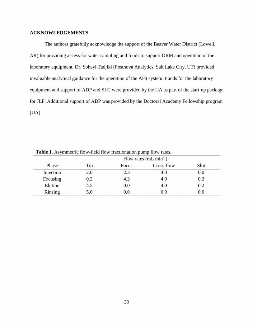
An AF4 sample run consists of four phases: (1) injection, (2) focusing, (3) elution, and

(4) rinsing. Individual pump flow rates varied between phases and shown in Table 1. Throughout

Phases 1-3, the detector flow rate was held constant at 0.3 mL min-1; in Phase 4, the flow passed

through the purge line to flush the system.

Ten-milliliter samples were injected into the AF4 channel using a bubble trap (Postnova

Analytics). This injection volume was chosen to balance adequate UV detection with

minimization of sample loss through the channel membrane during the injection and focusing

steps (Schimpf and Wahlund 1997). The tip pump flow was plumbed through the bubble trap and

carried the sample into the channel over 6–min. Concurrently, eluent from the focus pump was

supplied to the channel 18.5-cm from the inlet (LFP in Figure SM1), and a portion of this flow

traveled toward the channel inlet to keep sample macromolecules in the channel. Eluent exited

the channel during the injection step through the channel membrane by the action of the cross-

flow pump, which acted perpendicular to the long dimension of the channel. Sample injection

was followed by 6 minutes of focusing, designed to focus the sample into a uniform band near

the channel inlet (at z’ in Figure SM1). Next, in the transition phase, the focus pump flow was

19

decreased to zero as the tip pump ramped up to maintain the total flow over 1-min, followed by

the elution step and 5-min of rinsing.

Following the AF4 channel outlet, the fractionated sample flowed to an inline UV-diode

array detector (Agilent Technologies, G1315D), which collected UV data from 200-800 nm in 1

nm increments every 2-sec during the 20-min sample elution. UV254 was used to calculate the

diffusion coefficient distributions of the samples. Following the UV detector, the samples were

physically separated using a fraction collector (Agilent Technologies, Model 1364C). Three

equal-volume fractions (denoted F1, F2, and F3 herein) were collected in 2-mL pre-washed vials

beginning at 1-min elution and ending at 8-min elution. UV254 time series fractograms were

baseline corrected using the FFF Analysis software (Postnova Analytics v. 2.03A). The

fractogram data were used to determine the maximum UV254 peak heights (MaxUV) and area

under the curves (PeakArea), which was calculated using numerical integration with Simpson’s

method in the freeware program R (v. 2.10.1). Calculation of the diffusion coefficient from the

time-series data is detailed in Section 3.

2.5. Fluorescence

Fluorescence excitation-emission matrices (EEMs) were collected with a dual

monochromator fluorescence detector (Agilent Technologies, Model G1321A) equipped with a

static sample cuvette at 1-nm increments for excitation wavelengths between 200-400 nm and

emission wavelengths between 270-600 nm. The fluorescence cuvette was flushed thoroughly

with Milli-Q water between scans to prevent carryover and sample contamination. All scans

were corrected for first- and second-order Rayleigh and Raman water scattering using a

MATLAB ® Cleanscan program developed by Zepp et al. (2004). Cleanscan was applied to each

EEM and removed water scattering peaks and replaced them with a surface created by a 3-

20

dimensional Delauney interpolation algorithm. The areas of the EEMs over which Cleanscan

was invoked are shown in Fig. SM2.

Rather than relying on the peak picking methods used in previous works (e.g. Coble

(1996)), fluorescence PARAFAC modeling was used to identify the principal fluorophores and

their maximum intensities, FMAX , for all scatter-corrected EEMs. The EEMs were analyzed using

MATLAB ® functions contained in the DOM-Fluor toolbox (available for download at

http://www.models.life.ku.dk/algorithms). First, the fluorescence data was imported into

MATLAB ® as a collection of individual EEMs, stacked into a 3-dimensional structure using the

function Loading data for DOMfluor. PARAFAC models require the removal of outliers because

they can disproportionately influence the overall model output. Outliers can be the results of

measurement error (e.g. sample movement within the cuvette leading to “wrinkles” in the EEM)

or can be atypical samples. Such samples were identified visually and by running the function

OutlierTest. This test calculated and plotted leverages for each EEM, and identified those

considered as possible outliers based on high leverage values relative to the other samples. For

example, sample numbers 38, 81, and 100 in Fig. SM3 were identified as likely outliers. In cases

where EEMs were deemed to have both measurement errors and high leverages, these samples

were removed from the PARAFAC dataset. Next, the outlier program was used on the reduced

dataset, and additional samples were identified as requiring further investigation after an initial

estimate of the proper number of PARAFAC components. The Split-half analysis tool was used

for this step. The function, SplitData, divided the EEM dataset into two pairs of halves. These

halves were used in the functions SplitHalfAnalysis and SplitHalfValidation which compared the

shape of components derived from each half of the dataset with the other half’s components’

shapes. When component shapes from each half were identical, the corresponding model and

21

number of PARAFAC components was considered robust (Stedmon and Bro 2008). Figure SM4

shows an example of one unvalidated (the 4-Component) and two validated (the 3- and 5-

Component) split-half analysis models.

To ensure that all outliers were removed, questionable samples identified by the outlier

test were removed from the dataset one by one and split half analysis was repeated. Samples

were judged to be outliers if their removal changed the outcome of the split half analysis. This

resulted in a total of 87 EEMs in the PARAFAC model. In the case that more than one set of

components could be split half validated, the CompareSpecSSE function was used to plot the

sum of squared error (SSE) versus excitation and emission wavelengths (Stedmon and Markager

2005). The SSE for excitation and emission were normalized by the sum of squares for

excitation and emission and were plotted to give a visual indication of the level of residual

fluorescence compared to the measured fluorescence signal (Fig. SM5). This plot showed that

the 5-component model was superior to the 3-component model. As a final check, plots of

loadings versus excitation and emission wavelengths for each PARAFAC component were

generated and visually inspected. Stedmon and Bro (2008) suggested that these plots ideally

show emission loadings with a single peak and excitation and emission loadings slightly

overlapping. Discussion of these results is contained in Section 4.3.

Following the technique used by Fellman et al. (2008), the percent relative contribution

of each PARAFAC component was determined using FMAX values for each PARAFAC

component for all 87 EEMs. For a given EEM, FMAX for each component was divided by the

sum of FMAX for all the components (FMAX_TOT). For the whole water samples and AF4-generated

fractions, these quotients were averaged for each sample depth (3-, 10-, 18-m) and converted to a

percentage. This procedure simplified the interpretation of the PARAFAC data, and conveys the

22

relative contribution of the PARAFAC components at a given sample depth for each water

fraction.

3. CALCULATION

The diffusion coefficient, Df (in cm2 s-1) for the AF4-fractograms was calculated using

Eqn (1):

Eqn (1)

In Eqn (1), λ denotes the unitless retention parameter, VC is the cross-flow rate (4.0 mL min-1), w

is the experimentally determined channel thickness (0.041 cm, Section 2.3), and V0 is the

channel void volume, calculated by the product of channel thickness and the effective channel

area. The effective channel area, Aeff, was calculated as the channel area downstream of the

sample focus band, bz’, which was located 2.9 cm downstream of the channel inlet, as indicated

in the channel schematic (Fig. SM1). Using similar triangles, Aeff was calculated to be 32 cm2.

The effective channel area was also used to find α, a term used in the calculation of the void

time, t0, by Eqn (2).

Eqn (2)

In Eqn (2), b0 is the maximum channel width, bL is the width of the narrowest part of the

trapezoidal channel section, z’ is the distance from the channel inlet to the focusing band, Leff is

the effective channel length, and y is the channel area lost by the tapered channel (3.4 cm2). The

void time, t0, in seconds was then calculated with Eqn (3).

Eqn (3)

Df =λVC w2

V 0

α =1−

b0z'−(b0 − bL )(z')2

2⋅ Leff

− y

Aeff

t 0 =V 0

VC

ln(1+αVC

VOUT

)

23

In Eqn (3), VOUT is the volumetric flow rate of the channel outlet (0.5 mL min-1). The value of t0

was divided by the time series data to determine the unitless retention ratio values, R, shown in

Eqn (4), which is also equal to six times the retention parameter values, λ (Schimpf et al. 2000).

Eqn (4)

Values of λ were then used in Eqn (1) to determine the diffusion coefficient distribution. The

hydrodynamic diameter, dh, of the DOM was approximated from the molecular weight (MW)

using Eqn (5), similar to the procedure used by Howe and Clark (2002).

Eqn (5)

4. RESULTS AND DISCUSSION

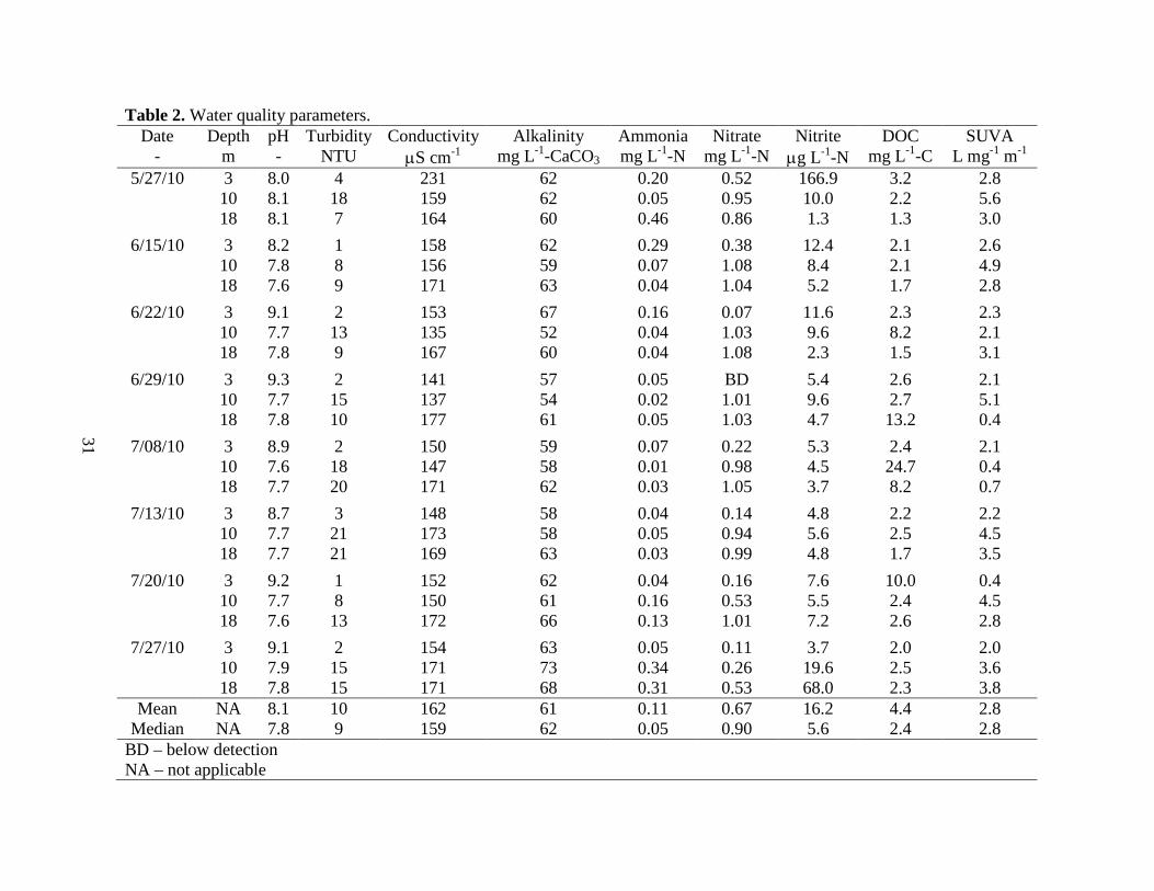
4.1. Water Quality Parameters

The raw water characteristics for the 24 BLW samples are reported in Table 2 along with

their mean and median values. All waters had a slightly alkaline pH, low turbidity, and low to

moderate alkalinity. Mean and median values were similar for pH (8.1 and 7.8), turbidity (10-

and 9-NTU), conductivity (162- and 159-µS cm-1), and alkalinity (61- and 62-mg L-1-CaCO3),

reflecting the tightly bunched nature of these metrics amongst the water samples. Conversely,

mean and median values differed for ammonia (0.11- and 0.05-mg L-1-N), nitrate (0.67- and

0.90-mg L-1-N), nitrite (16.2- and 5.6-µg L-1-N), and DOC (4.4- and 2.4-mg L-1-C), indicating

these metrics were skewed by a handful of low (for nitrate) and high (for ammonia, nitrite, and

DOC) values. Fig. SM6 shows a pair-wise scatter-plot for the water quality parameters. While

there were no temporal trends (those with Date), spatial trends (those with Depth) were only

apparent for pH, turbidity, and nitrate (second column in Fig. SM6). Values for pH were higher

at 3-m than at 10- and 18-m; conversely, turbidities were lower at 3-m compared to the 10- and

18-m depths likely because of higher sediment loadings near the bottom of the reservoir.

t 0

tr

= R = 6⋅ λ

dh = 0.09⋅ (MW )0.44

24

Total iron was not reported in Table 2 because these values were below 0.33 mg L-1-Fe,

with 22 of the 24 samples below the estimated detection limit (0.20 mg L-1-Fe) of the Hach

FerroVer test. Weishaar (2003) evaluated potential interferences of background analytes on

UV254 and determined that a UV254 of 0.01 required 1 mg L-1-Fe total iron and in excess of 23

mg L-1-N nitrate. Given the iron and nitrate concentrations in the sample waters were below

these thresholds, we concluded that the UV254 measurements (for the SUVA calculations and

AF4 fractograms) were not impacted by dissolved iron and nitrate.

Interestingly, the four samples with high DOC values (those above 8 mg L-1 C in Table 2)

all had below average alkalinity values (< 62 mg L-1-CaCO3), suggesting the carbonate system

controlled the alkalinity of all lake water samples and the diverse groups of weak acids present in

the DOM did not contribute significantly to alkalinity. SUVA, calculated as UV254 divided by the

product of the UV cell path length (0.01-m) and DOC, varied from 0.4- to 5.6-L mg C-1 m-1.

Weishaar et al. (2003) showed that SUVA had a strong positive correlation with 13C-NMR (a

direct measure of DOM aromaticity), but was weakly correlated with trihalomethane formation

(a principal group of DBPs), suggesting non-aromatic compounds present in DOM mixtures

contributed significantly to DBP formation. Therefore, for the waters in this study, the range of

SUVA values suggest a wide array of CDOM aromaticities, but cannot be used to reliably

estimate the DBP formation potential.

4.2. AF4-Fractograms

In Fig 1., AF4-fractograms were plotted as a function of elution time (tr) and diffusion

coefficient (Df). Fig. 1A-B show the fractograms of 1.1-, 4.2-, and 10.6-kDa polystyrene

sulfonate sodium salt (PSS) standards (ca. 30 mg L-1 in 0.001 M NaCl), which other researchers

(Beckett et al. 1987; Assemi et al. 2004) have recommended as a molecular weight surrogate for

25

humic substances. For each PSS standard, Df at the peak maximum was plotted against its

molecular weight and compared to PSS data from other research groups (Beckett et al. 1987;

Dycus et al. 1995; van Bruijnsvoort et al. 2001; Assemi et al. 2004) (Fig. 2). These data show

that the Df values determined here were bracketed by those reported in the literature. The spread

in these data between research groups (approximately one-half an order of magnitude in log Df

for log MW values less than 4.0) can likely be attributed to different background electrolyte

compositions.

The AF4-fractogram of Suwannee River natural organic matter (SRNOM, International

Humic Substances Society, Atlanta, GA, Cat. No. 1R101N; ca. 4 mg L-1 in 0.001 M NaCl) is

also shown in Fig. 1A-B. This peak was broader than those of the PSS standards, with a peak

maximum near that of the 4.2 kDa PSS standard (tr = 4.2 min, Fig. 1A; Df = 2.4×10-6 cm2s-1, Fig.

1B) and a “shoulder-like” feature indicating the presence of CDOM smaller than 1.1 kDa PSS (tr

= 2 min, Fig. 1A; Df = 5.0×10-6 cm2s-1, Fig. 1B). This broad range of Df determined here for

SRNOM (~1.0-5.0×10-6 cm2s-1) was smaller than that reported by Moon et al. (2006) of 4.1-

5.5×10-6 cm2s-1 (Table 3). However, when coupled with the results of the PSS standards (Fig. 2),

it can concluded that the AF4 methods used here produced similar results to those reported by

other research groups, for which a variety of preparative and analytical techniques were used.

Fig. 1C-D show AF4-fractograms for BLW CDOM samples collected on July 8, 2010 at

depths of 3-, 10-, and 18-m. The trends shown in Fig. 1D were typical of the other 21

fractograms (Fig. SM7), with BLW CDOM at the 10-m depth having greater UV254 peak

maximums (with the exception of the first two sampling days) than the samples collected at 3-

and 18-m depths. All fractograms had a small, shoulder-like void peak at an elution time of 1.5-

min followed by a larger, broad sample peak between 2- and 6-min. The grey boxes in Fig. 1C

26

denote the three fractions (F1-F3) that were collected for subsequent fluorescence analyses

(Section 4.3). For the 24 BLW CDOM fractograms, the Df peak maximum ranged from 3.5- to

2.8- ×10-6 cm2 s-1. The peak maximums of the three PSS standards were appended as dashed

lines in Fig. 1D, and indicate the BLW CDOM was most similar in diffusivity to that of the 1.1-

kDa PSS standard. The approximate molecular weight range of the BLW CDOM was calculated

by comparison to the PSS data. Here, the log-linear trend line for the three PSS standards (Fig. 2,

R2 = 1, P < 0.02, slope: -0.21, y-intercept: -4.86) was used with the range of Df peak maximums

(3.5- to 2.8- ×10-6 cm2 s-1) to determine the molecular weight of BLW CDOM (680-1,950 Da).

Using Eqn (5), this corresponded to a size range of 1.6-2.5 nm. The molecular weights and

diffusivities for the BLW CDOM were compared to literature-reported values for the various

humic substances (Table 3), which, on balance, indicated the results determined here were within

the reported ranges of CDOM using a variety of preparative and analytical techniques. Thus, it

can be concluded that BLW CDOM was composed primarily of relatively low molecular weight

aromatic carbon-containing molecules (680-1,950 Da) with diffusivities between 3.5- to 2.8-

×10-6 cm2 s-1. However, it should be stressed that UV254 was used to monitor the AF4-

fractrogram output, and as such, non-aromatic containing DOM was not characterized. As such,

there is a possibility that colloidal DOM (3,000-100,000 Da), much larger than the fraction found

here, was also present in the BLW samples, as reported by Howe and Clark (2002) in their

membrane fouling study, but could not be “seen” by UV254.

The AF4-fractogram data (the UV254 peak maximums, MaxUV, and the area under each

curve, PeakArea) were compared to select water quality data (DOC and SUVA) as a function of

sample date and depth. Fig. 3 shows a pair-wise scatter-plot of these data, which indicated there

were no temporal trends (those with Date). Conversely, trends with sample Depth were apparent

27

for SUVA, MaxUV and PeakArea (the second column of Fig. 3). As indicated by the trend lines,

all these metrics were on balance higher for the 10-m samples compared to the 3- and 18-m

samples. Given SUVA is a surrogate for aromatic carbon (Weishaar et al. 2003), these results

indicate that the nature of the CDOM pool in the Beaver Reservoir was stratified by depth over

the 8-week sampling period. The strong linear relationship between MaxUV and PeakArea (R2 =

0.97, P < 0.001) indicated that only one of these metrics needed to be determined to adequately

describe the AF4-fractogram data; for simplicity, MaxUV was selected for further analyses. For

the 24 lake water samples, MaxUV varied from 20-85 absorbance units (data not shown) and

was uncorrelated with DOC (Fig. 3). However, MaxUV and SUVA had a weak positive

correlation (Fig. 3, R2 = 0.21, P = 0.024), suggesting that MaxUV would not be a good surrogate

of CDOM aromaticity, but may be helpful in assessing CDOM reactivity in DBP studies.

4.3. Fluorescence-PARAFAC Analyses

Fluorescence excitation-emission matrices (EEMs) of the 24 whole water samples and 72

AF4-generated fractions were processed as described in Section 2.4. PARAFAC modeling began

with the 96 samples, eleven of which were removed based on the protocol detailed in Section

2.4. Split half analyses on the remaining 85 samples showed that three- and five-component

models were appropriate for the dataset (Fig. SM4). Fig. SM5 shows the integrated excitation

and emission spectra for the sum of squared errors for three- and five-component models and the

relative SSE normalized by the total sum of squares. The presence of peaks in these spectra

corresponds to regions of the EEMs that are less well described by the model. The results in Fig.

SM5 show that a five-component model was superior to the three-component model over the

range of excitation and emission wavelengths. For the five-component model, the normalized

residual excitation between 200- and 375-nm was less than 1% of the measured signal; similarly,

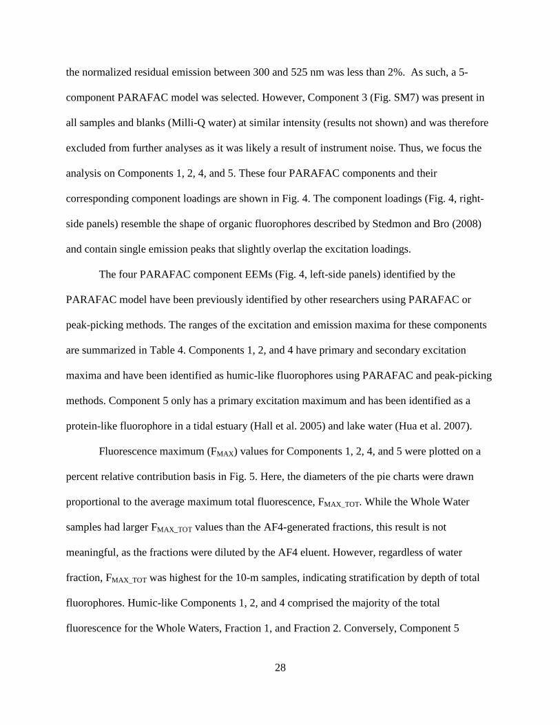
28

the normalized residual emission between 300 and 525 nm was less than 2%. As such, a 5-

component PARAFAC model was selected. However, Component 3 (Fig. SM7) was present in

all samples and blanks (Milli-Q water) at similar intensity (results not shown) and was therefore

excluded from further analyses as it was likely a result of instrument noise. Thus, we focus the

analysis on Components 1, 2, 4, and 5. These four PARAFAC components and their

corresponding component loadings are shown in Fig. 4. The component loadings (Fig. 4, right-

side panels) resemble the shape of organic fluorophores described by Stedmon and Bro (2008)

and contain single emission peaks that slightly overlap the excitation loadings.

The four PARAFAC component EEMs (Fig. 4, left-side panels) identified by the

PARAFAC model have been previously identified by other researchers using PARAFAC or

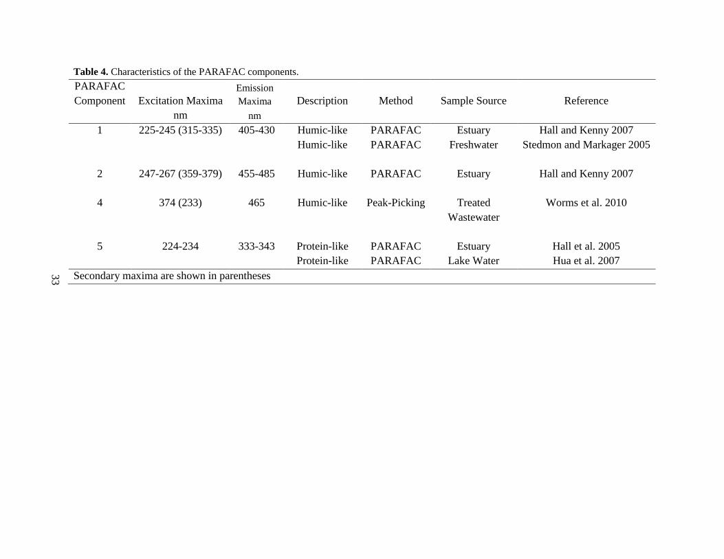
peak-picking methods. The ranges of the excitation and emission maxima for these components

are summarized in Table 4. Components 1, 2, and 4 have primary and secondary excitation

maxima and have been identified as humic-like fluorophores using PARAFAC and peak-picking

methods. Component 5 only has a primary excitation maximum and has been identified as a

protein-like fluorophore in a tidal estuary (Hall et al. 2005) and lake water (Hua et al. 2007).

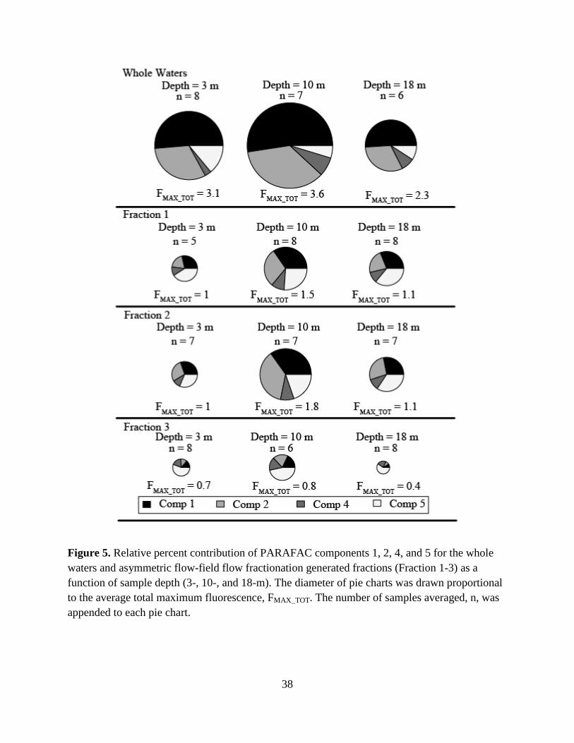
Fluorescence maximum (FMAX ) values for Components 1, 2, 4, and 5 were plotted on a

percent relative contribution basis in Fig. 5. Here, the diameters of the pie charts were drawn

proportional to the average maximum total fluorescence, FMAX_TOT. While the Whole Water

samples had larger FMAX_TOT values than the AF4-generated fractions, this result is not

meaningful, as the fractions were diluted by the AF4 eluent. However, regardless of water

fraction, FMAX_TOT was highest for the 10-m samples, indicating stratification by depth of total

fluorophores. Humic-like Components 1, 2, and 4 comprised the majority of the total

fluorescence for the Whole Waters, Fraction 1, and Fraction 2. Conversely, Component 5

29

dominated Fraction 3, indicating this protein-like fluorophore was present in relatively large-

sized DOM. Further, Component 5 was in least abundance for the 10-m depth samples for all

water fractions, indicating stratification by depth of the type of fluorophores.

5. CONCLUSIONS

The physicochemical properties of CDOM at three depths in the Beaver Lake Reservoir

(Lowell, AR) were studied between May-July, 2010. BLW CDOM, as measured by AF4-UV254

and SUVA, showed that the 10-m depth samples had higher intensities and SUVA values than

did the 3- and 18-m depth samples. For the 24 BLW CDOM samples, the diffusion coefficient

peak maximums ranged from 2.8- to 3.5×10-6 cm2 s-1, which corresponded to a molecular weight

range of 680-1,950 Da and a size of 1.6-2.5 nm. As such, the BLW CDOM was comprised of

relatively low molecular weight aromatic carbon-containing molecules with no measured

colloidal fraction (3,000-100,000 Da). Fluorescence-PARAFAC modeling of the whole water

samples and AF4-generated fractions yielded five principal components. However, Component 3

was attributed to instrument noise and discarded. PARAFAC Components 1, 2, and 4 had

primary and secondary excitation maxima and resembled humic-like fluorophores identified

previously by either PARAFAC or peak-picking techniques. Conversely, Component 5 had a

single excitation maxima and was most similar to a protein-like fluorophore identified in

estuarine and lake water samples. Samples from the 10-m sampling depth had the highest total

fluorescence, echoing the AF4-UVA254 results, and adding further weight-of-evidence to the

conclusion that the BLW CDOM was stratified by depth. Further, the relative percent

contribution of each fluorophore varied by depth, indicating that the type of fluorophores were

stratified by depth. The stratification of BLW CDOM shown here has potentially important

implications for drinking water utilities that aim to reduce formation of disinfection byproducts.

30

ACKNOWLEDGEMENTS

The authors gratefully acknowledge the support of the Beaver Water District (Lowell,

AR) for providing access for water sampling and funds to support DRM and operation of the

laboratory equipment. Dr. Soheyl Tadjiki (Postnova Analytics, Salt Lake City, UT) provided

invaluable analytical guidance for the operation of the AF4 system. Funds for the laboratory

equipment and support of ADP and SLC were provided by the UA as part of the start-up package

for JLF. Additional support of ADP was provided by the Doctoral Academy Fellowship program

(UA).

Table 1. Asymmetric flow-field flow fractionation pump flow rates.

Phase Flow rates (mL min-1)

Tip Focus Cross-flow Slot Injection 2.0 2.3 4.0 0.0 Focusing 0.2 4.3 4.0 0.2 Elution 4.5 0.0 4.0 0.2 Rinsing 5.0 0.0 0.0 0.0

31

Table 2. Water quality parameters. Date Depth pH Turbidity Conductivity Alkalinity Ammonia Nitrate Nitrite DOC SUVA

- m - NTU µS cm-1 mg L-1-CaCO3 mg L-1-N mg L-1-N µg L-1-N mg L-1-C L mg-1 m-1 5/27/10 3 8.0 4 231 62 0.20 0.52 166.9 3.2 2.8

10 8.1 18 159 62 0.05 0.95 10.0 2.2 5.6 18 8.1 7 164 60 0.46 0.86 1.3 1.3 3.0

6/15/10 3 8.2 1 158 62 0.29 0.38 12.4 2.1 2.6 10 7.8 8 156 59 0.07 1.08 8.4 2.1 4.9 18 7.6 9 171 63 0.04 1.04 5.2 1.7 2.8

6/22/10 3 9.1 2 153 67 0.16 0.07 11.6 2.3 2.3 10 7.7 13 135 52 0.04 1.03 9.6 8.2 2.1 18 7.8 9 167 60 0.04 1.08 2.3 1.5 3.1

6/29/10 3 9.3 2 141 57 0.05 BD 5.4 2.6 2.1 10 7.7 15 137 54 0.02 1.01 9.6 2.7 5.1 18 7.8 10 177 61 0.05 1.03 4.7 13.2 0.4

7/08/10 3 8.9 2 150 59 0.07 0.22 5.3 2.4 2.1 10 7.6 18 147 58 0.01 0.98 4.5 24.7 0.4 18 7.7 20 171 62 0.03 1.05 3.7 8.2 0.7

7/13/10 3 8.7 3 148 58 0.04 0.14 4.8 2.2 2.2 10 7.7 21 173 58 0.05 0.94 5.6 2.5 4.5 18 7.7 21 169 63 0.03 0.99 4.8 1.7 3.5

7/20/10 3 9.2 1 152 62 0.04 0.16 7.6 10.0 0.4 10 7.7 8 150 61 0.16 0.53 5.5 2.4 4.5 18 7.6 13 172 66 0.13 1.01 7.2 2.6 2.8

7/27/10 3 9.1 2 154 63 0.05 0.11 3.7 2.0 2.0 10 7.9 15 171 73 0.34 0.26 19.6 2.5 3.6 18 7.8 15 171 68 0.31 0.53 68.0 2.3 3.8

Mean NA 8.1 10 162 61 0.11 0.67 16.2 4.4 2.8 Median NA 7.8 9 159 62 0.05 0.90 5.6 2.4 2.8

BD – below detection NA – not applicable

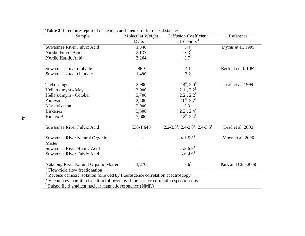
32

Table 3. Literature-reported diffusion coefficients for humic substances Sample Molecular Weight Diffusion Coefficient Reference

Daltons ×106 cm2 s-1 Suwannee River Fulvic Acid 1,340 3.4† Dycus et al. 1995 Nordic Fulvic Acid 2,137 3.3† Nordic Humic Acid 3,264 2.7† Suwannee stream fulvate 860 4.1 Beckett et al. 1987 Suwannee stream humate 1,490 3.2 Trehorningen 2,900 2.4‡, 2.6§ Lead et al. 1999 Hellerudmyra - May 3,900 2.1‡, 2.2§ Hellerudmyra - October 3,700 2.2‡, 2.2§ Aurevann 2,400 2.6‡, 2.7§ Maridulsvann 2,900 2.3‡ Birkenes 3,500 2.2‡, 2.4§ Humex B 3,600 2.2‡, 2.4§ Suwannee River Fulvic Acid 530-1,640 2.2-3.3†; 2.4-2.8‡; 2.4-3.5¶ Lead et al. 2000 Suwannee River Natural Organic Matter

- 4.1-5.5† Moon et al. 2006

Suwannee River Humic Acid - 4.5-5.8† Suwannee River Fulvic Acid - 3.6-4.6† Nakdong River Natural Organic Matter 1,270 5.6† Park and Cho 2008 † Flow-field flow fractionation ‡ Reverse osmosis isolation followed by fluorescence correlation spectroscopy § Vacuum evaporation isolation followed by fluorescence correlation spectroscopy ¶ Pulsed field gradient nuclear magnetic resonance (NMR)

33

Table 4. Characteristics of the PARAFAC components.

PARAFAC Component Excitation Maxima

Emission Maxima Description Method Sample Source Reference

nm nm 1 225-245 (315-335) 405-430 Humic-like PARAFAC Estuary Hall and Kenny 2007 Humic-like PARAFAC Freshwater Stedmon and Markager 2005 2 247-267 (359-379) 455-485 Humic-like PARAFAC Estuary Hall and Kenny 2007 4 374 (233) 465 Humic-like Peak-Picking Treated

Wastewater Worms et al. 2010

5 224-234 333-343 Protein-like PARAFAC Estuary Hall et al. 2005 Protein-like PARAFAC Lake Water Hua et al. 2007

Secondary maxima are shown in parentheses

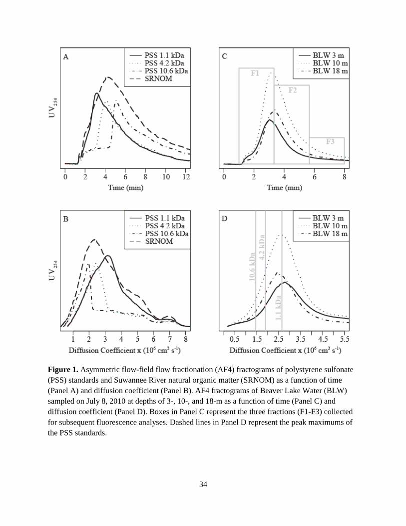
34

Figure 1. Asymmetric flow-field flow fractionation (AF4) fractograms of polystyrene sulfonate (PSS) standards and Suwannee River natural organic matter (SRNOM) as a function of time (Panel A) and diffusion coefficient (Panel B). AF4 fractograms of Beaver Lake Water (BLW) sampled on July 8, 2010 at depths of 3-, 10-, and 18-m as a function of time (Panel C) and diffusion coefficient (Panel D). Boxes in Panel C represent the three fractions (F1-F3) collected for subsequent fluorescence analyses. Dashed lines in Panel D represent the peak maximums of the PSS standards.

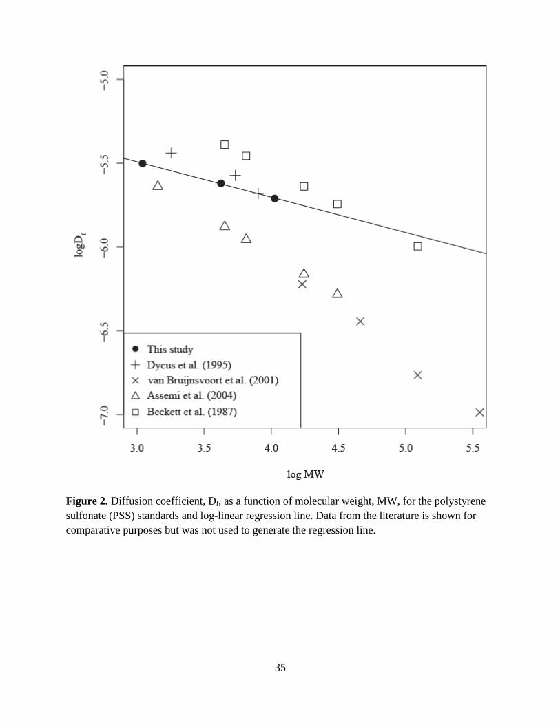
35

Figure 2. Diffusion coefficient, Df, as a function of molecular weight, MW, for the polystyrene sulfonate (PSS) standards and log-linear regression line. Data from the literature is shown for comparative purposes but was not used to generate the regression line.

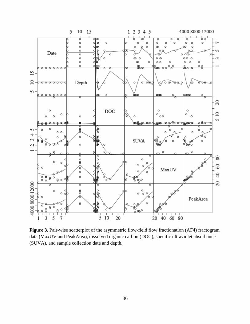
Figure 3. Pair-wise scatterplot of the asymmetric flowdata (MaxUV and PeakArea), dissolved orga(SUVA), and sample collection date and depth.

36

wise scatterplot of the asymmetric flow-field flow fractionation (AF4) fractogram data (MaxUV and PeakArea), dissolved organic carbon (DOC), specific ultraviolet absorbance (SUVA), and sample collection date and depth.

field flow fractionation (AF4) fractogram nic carbon (DOC), specific ultraviolet absorbance

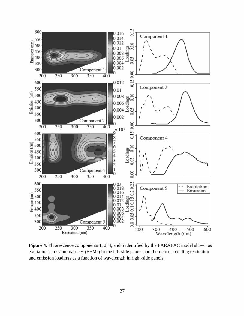
Figure 4. Fluorescence components 1, 2, 4, and 5 identified by the PARAFAC model shown as excitation-emission matrices (EEMs) in the leftand emission loadings as a function of wavelength in right

37

Fluorescence components 1, 2, 4, and 5 identified by the PARAFAC model shown as emission matrices (EEMs) in the left-side panels and their corresponding excitation

and emission loadings as a function of wavelength in right-side panels.

Fluorescence components 1, 2, 4, and 5 identified by the PARAFAC model shown as side panels and their corresponding excitation

38

Figure 5. Relative percent contribution of PARAFAC components 1, 2, 4, and 5 for the whole waters and asymmetric flow-field flow fractionation generated fractions (Fraction 1-3) as a function of sample depth (3-, 10-, and 18-m). The diameter of pie charts was drawn proportional to the average total maximum fluorescence, FMAX_TOT. The number of samples averaged, n, was appended to each pie chart.

39

6. REFERENCES

Alasonati, E., Slaveykova, V. I., Gallard, H., Croue, J. P. and Benedetti, M. F., 2010. Characterization of the colloidal organic matter from the Amazonian basin by asymmetrical flow field-flow fractionation and size exclusion chromatography. Water Research 44 (1), 223-231.


Assemi, S., Newcombe, G., Hepplewhite, C. and Beckett, R., 2004. Characterization of natural organic matter fractions separated by ultrafiltration using flow field-flow fractionation. Water Research 38 (6), 1467-1476.

Baalousha, M., Kammer, F. V. D., Motelica-Heino, M. and Le Coustumer, P., 2005. Natural sample fractionation by F1FFF-MALLS-TEM: Sample stabilization, preparation, pre-concentration and fractionation. Journal of Chromatography A 1093 (1-2), 156-166.

Baalousha, M. and Lead, J. R., 2007. Characterization of natural aquatic colloids (< 5 nm) by flow-field flow fractionation and atomic force microscopy. Environmental Science & Technology 41 (4), 1111-1117.

Beckett, R., Jue, Z. and Giddings, J. C., 1987. Determination of molecular weight distributions of fulvic and humic acids using flow field-flow fractionation. Environmental Science & Technology 21 (3), 289-295.

Boehme, J. and Wells, M., 2006. Fluorescence variability of marine and terrestrial colloids: Examining size fractions of chromophoric dissolved organic matter in the Damariscotta River estuary. Marine Chemistry 101 (1-2), 95-103.

Cabaniss, S. E., Zhou, Q. H., Maurice, P. A., Chin, Y. P. and Aiken, G. R., 2000. A log-normal distribution model for the molecular weight of aquatic fulvic acids. Environmental Science & Technology 34 (6), 1103-1109.

Cawley, K. M., Hakala, J. A. and Chin, Y. P., 2009. Evaluating the triplet state photoreactivity of dissolved organic matter isolated by chromatography and ultrafiltration using an alkylphenol probe molecule. Limnology and Oceanography-Methods 7, 391-398.

Chatterjee, A., 1964. Diffusion Studies of Bovine Plasma Albumin at 25° with the Help of Jamin Interference Optics. Journal of the American Chemical Society 86 (18), 3640-3642.

Chu, W.-H., Gao, N.-Y., Deng, Y. and Krasner, S. W., 2010. Precursors of Dichloroacetamide, an Emerging Nitrogenous DBP Formed during Chlorination or Chloramination. Environmental Science & Technology 44 (10), 3908-3912.


40


Dubascoux, S., Von Der Kammer, F., Le Hecho, I., Gautier, M. P. and Lespes, G., 2008. Optimisation of asymmetrical flow field flow fractionation for environmental nanoparticles separation. Journal of Chromatography A 1206 (2), 160-165.

Dycus, P. J. M., Healy, K. D., Stearman, G. K. and Wells, M. J. M., 1995. Diffusion-coefficients and molecular-weight distributions of humic and fulvic-acids determined by flow field-flow fractionation. Separation Science and Technology 30 (7-9), 1435-1453.

Eaton, A. D., Clesceri, L. S., Rice, E. W. and Greenberg, A. E., Eds. (2005). Standard methods for the examination of water & wastewater. Washington, DC, American Public Health Association

Fellman, J. B., D'Amore, D. V., Hood, E. and Boone, R. D., 2008. Fluorescence characteristics and biodegradability of dissolved organic matter in forest and wetland soils from coastal temperate watersheds in southeast Alaska. Biogeochemistry 88 (2), 169-184.

Floge, S. A. and Wells, M. L., 2007. Variation in colloidal chromophoric dissolved organic matter in the Damariscotta Estuary, Maine. Limnology and Oceanography 52 (1), 32-45.

Gadmar, T. C., Vogt, R. D. and Evje, L., 2005. Artifacts in XAD-8 NOM fractionation. International Journal of Environmental Analytical Chemistry 85 (6), 365-376.

Giddings, J. C., 1993. Field-flow fractionation - Analysis of macromolecular, colloidal, and particulate materials. Science 260 (5113), 1456-1465.


Hall, G. J. and Kenny, J. E., 2007. Estuarine water classification using EEM spectroscopy and PARAFAC-SIMCA. Analytica Chimica Acta 581 (1), 118-124.

Howe, K. J. and Clark, M. M., 2002. Fouling of microfiltration and ultrafiltration membranes by natural waters. Environmental Science & Technology 36 (16), 3571-3576.

Hua, B., Dolan, F., McGhee, C., Clevenger, T. E. and Deng, B., 2007. Water-source characterization and classification with fluorescence EEM spectroscopy: PARAFAC analysis. International Journal of Environmental Analytical Chemistry 87 (2), 135-147.

Hua, B., Veum, K., Yang, J., Jones, J. and Deng, B. L., 2010. Parallel factor analysis of fluorescence EEM spectra to identify THM precursors in lake waters. Environmental Monitoring and Assessment 161 (1-4), 71-81.

41

Huguet, A., Vacher, L., Relexans, S., Saubusse, S., Froidefond, J. M. and Parlanti, E., 2009. Properties of fluorescent dissolved organic matter in the Gironde Estuary. Organic Geochemistry 40 (6), 706-719.

Johnstone, D. W. and Miller, C. M., 2009. Fluorescence Excitation-Emission Matrix Regional Transformation and Chlorine Consumption to Predict Trihalomethane and Haloacetic Acid Formation. Environmental Engineering Science 26 (7), 1163-1170.



Kitis, M., Karanfil, T., Kilduff, J.E., Wigton, A., 2001. The reactivity of natural organic matter to disinfection byproducts formation and its relation to specific ultraviolet absorbance. Water Science and Technology 43 (2), 9-16.

Korshin, G. V., Benjamin, M. M., Chang, H. S. and Gallard, H., 2007. Examination of NOM chlorination reactions by conventional and stop-flow differential absorbance spectroscopy. Environmental Science & Technology 41 (8), 2776-2781.

Krachler, R., Krachler, R. F., von der Kammer, F., Suephandag, A., Jirsa, F., Ayromlou, S., Hofmann, T. and Keppler, B. K., 2010. Relevance of peat-draining rivers for the riverine input of dissolved iron into the ocean. Science of the Total Environment 408 (11), 2402-2408.

Lead, J. R., Balnois, E., Hosse, M., Menghetti, R. and Wilkinson, K. J., 1999. Characterization of Norwegian natural organic matter: Size, diffusion coefficients, and electrophoretic mobilities. Environment International 25 (2-3),245-258.

Lead, J. R., Wilkinson, K. J., Balnois, E., Cutak, B. J., Larive, C. K., Assemi, S. and Beckett, R., 2000. Diffusion coefficients and polydispersities of the Suwannee River fulvic acid: Comparison of fluorescence correlation spectroscopy, pulsed-field gradient nuclear magnetic resonance, and flow field-flow fractionation. Environmental Science & Technology 34 (16), 3508-3513.

LeChevallier, M. W., Welch, N. J. and Smith, D. B., 1996. Full-scale studies of factors related to coliform regrowth in drinking water. Applied and Environmental Microbiology 62 (7), 2201-2211.

Moon, J., Kim, S. H. and Cho, J., 2006. Characterizations of natural organic matter as nano particle using flow field-flow fractionation. Colloids and Surfaces a-Physicochemical and Engineering Aspects 287 (1-3), 232-236.

42

Park, N. and Cho, J., 2008. Natural organic matter diffusivity for transport characterizations in nanofiltration and ultrafiltration memrbanes. Journal of Membrane Science 315 (1-2), 133-140.

Prestel, H., Niessner, R. and Panne, U., 2006. Increasing the sensitivity of asymmetrical flow field-flow fractionation: Slot outlet technique. Analytical Chemistry 78 (18), 6664-6669.

Reszat, T. N. and Hendry, M. J., 2005. Characterizing dissolved organic carbon using asymmetrical flow field-flow fractionation with on-line UV and DOC detection. Analytical Chemistry 77 (13), 4194-4200.

Rook, J. J., 1977. Chlorination reactions of fulvic acids in natural waters. Environmental Science & Technology 11 (5), 478-482.

Santschi, P. H., Roberts, K. A. and Guo, L., 2002. Organic Nature of Colloidal Actinides Transported in Surface Water Environments. Environmental Science & Technology 36 (17), 3711-3719.

Schimpf, M. E., Caldwell, K. D. and Giddings, J. C., Eds. (2000). Field-flow fractionation handbook, John Wiley & Sons, Inc.


Sen, S., Haggard, B. E., Chaubey, I., Brye, K. R., Costello, T. A. and Matlock, M. D., 2007. Sediment phosphorus release at Beaver Reservoir, northwest Arkansas, USA, 2002-2003: A preliminary investigation. Water Air and Soil Pollution 179 (1-4), 67-77.

Stedmon, C. A. and Bro, R., 2008. Characterizing dissolved organic matter fluorescence with parallel factor analysis: a tutorial. Limnology and Oceanography-Methods 6, 572-579.

Stedmon, C. A. and Markager, S., 2005. Resolving the variability in dissolved organic matter fluorescence in a temperate estuary and its catchment using PARAFAC analysis. Limnology and Oceanography 50 (2), 686-697.

Stolpe, B., Guo, L. D., Shiller, A. M. and Hassellov, M., 2010. Size and composition of colloidal organic matter and trace elements in the Mississippi River, Pearl River and the northern Gulf of Mexico, as characterized by flow field-flow fractionation. Marine Chemistry 118 (3-4), 119-128.

van Bruijnsvoort, M., Tijssen, R. and Kok, W. T., 2001. Assessment of the diffusional behavior of polystyrene sulfonates in the dilute regime by hollow-fiber flow field flow fractionation. Journal of Polymer Science Part B: Polymer Physics 39 (15), 1756-1765.

Wahlund, K. G. and Giddings, J. C., 1987. Properties of an asymmetrical flow field-flow fractionation channel having one permeable wall. Analytical Chemistry 59 (9), 1332-1339.

43

Weishaar, J. L., Aiken, G. R., Bergamaschi, B. A., Fram, M. S., Fujii, R. and Mopper, K., 2003. Evaluation of specific ultraviolet absorbance as an indicator of the chemical composition and reactivity of dissolved organic carbon. Environmental Science & Technology 37 (20), 4702-4708.

Worms, I. A. M., Szigeti, Z. A. G., Dubascoux, S., Lespes, G., Traber, J., Sigg, L. and Slaveykova, V. I., 2010. Colloidal organic matter from wastewater treatment plant effluents: Characterization and role in metal distribution. Water Research 44 (1), 340-350.

Yang, X., Shang, C., Lee, W., Westerhoff, P. and Fan, C. H., 2008. Correlations between organic matter properties and DBP formation during chloramination. Water Research 42 (8-9), 2329-2339.


Zepp, R. G., Sheldon, W. M. and Moran, M. A., 2004. Dissolved organic fluorophores in southeastern US coastal waters: correction method for eliminating Rayleigh and Raman scattering peaks in excitation-emission matrices. Marine Chemistry 89 (1-4), 15-36.

44

APPENDIX 1

Supporting Material for

“Coupling Asymmetric Flow-Field Flow Fractionation and Fluorescence Parallel Factor

Analysis Reveals Stratification of Dissolved Organic Matter in a Drinking Water

Reservoir”

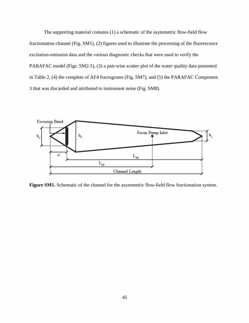
45

The supporting material contains (1) a schematic of the asymmetric flow-field flow

fractionation channel (Fig. SM1), (2) figures used to illustrate the processing of the fluorescence

excitation-emission data and the various diagnostic checks that were used to verify the

PARAFAC model (Figs. SM2-5), (3) a pair-wise scatter plot of the water quality data presented

in Table 2, (4) the complete of AF4 fractograms (Fig. SM7), and (5) the PARAFAC Component

3 that was discarded and attributed to instrument noise (Fig. SM8).

Figure SM1. Schematic of the channel for the asymmetric flow-field flow fractionation system.

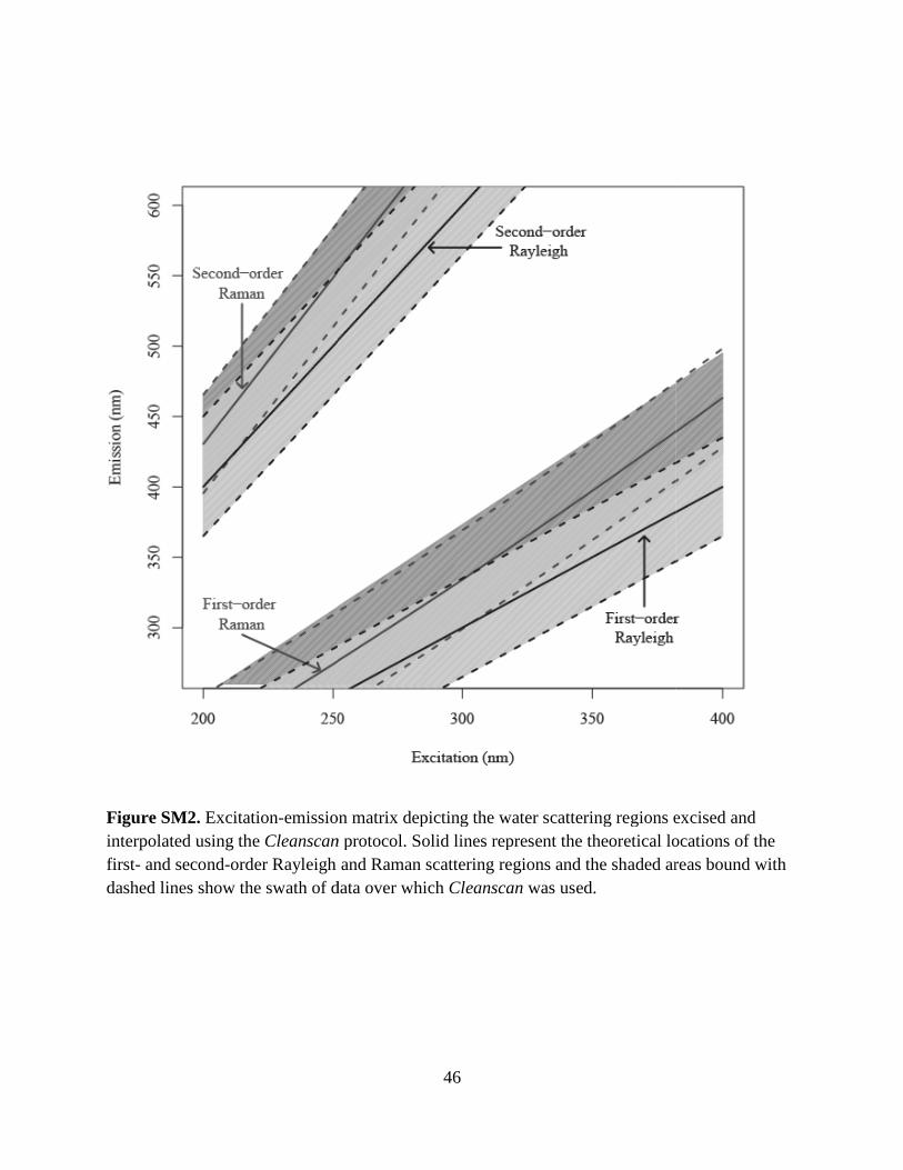
Figure SM2. Excitation-emission matrixinterpolated using the Cleanscanfirst- and second-order Rayleigh and Raman scattering regions and the shaded areas bound with dashed lines show the swath of data over which

46

emission matrix depicting the water scattering regions excised and Cleanscan protocol. Solid lines represent the theoretical locations of the

order Rayleigh and Raman scattering regions and the shaded areas bound with show the swath of data over which Cleanscan was used.

depicting the water scattering regions excised and protocol. Solid lines represent the theoretical locations of the

order Rayleigh and Raman scattering regions and the shaded areas bound with

Figure SM3. Leverage plots for the excitationPARAFAC data array.

47

Leverage plots for the excitation-emission matrices contained in the initial emission matrices contained in the initial

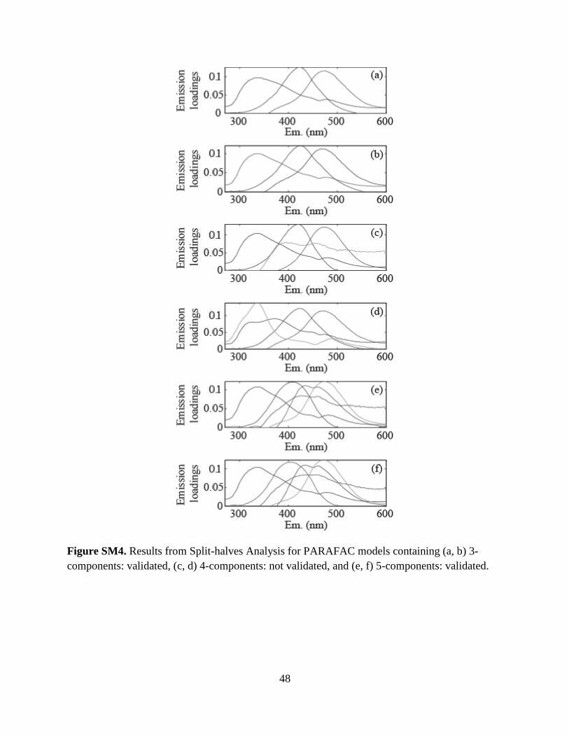
Figure SM4. Results from Split-components: validated, (c, d) 4-components: not validated, and (e, f) 5

48

-halves Analysis for PARAFAC models containing (a, b)components: not validated, and (e, f) 5-components: validated.halves Analysis for PARAFAC models containing (a, b) 3-

components: validated.

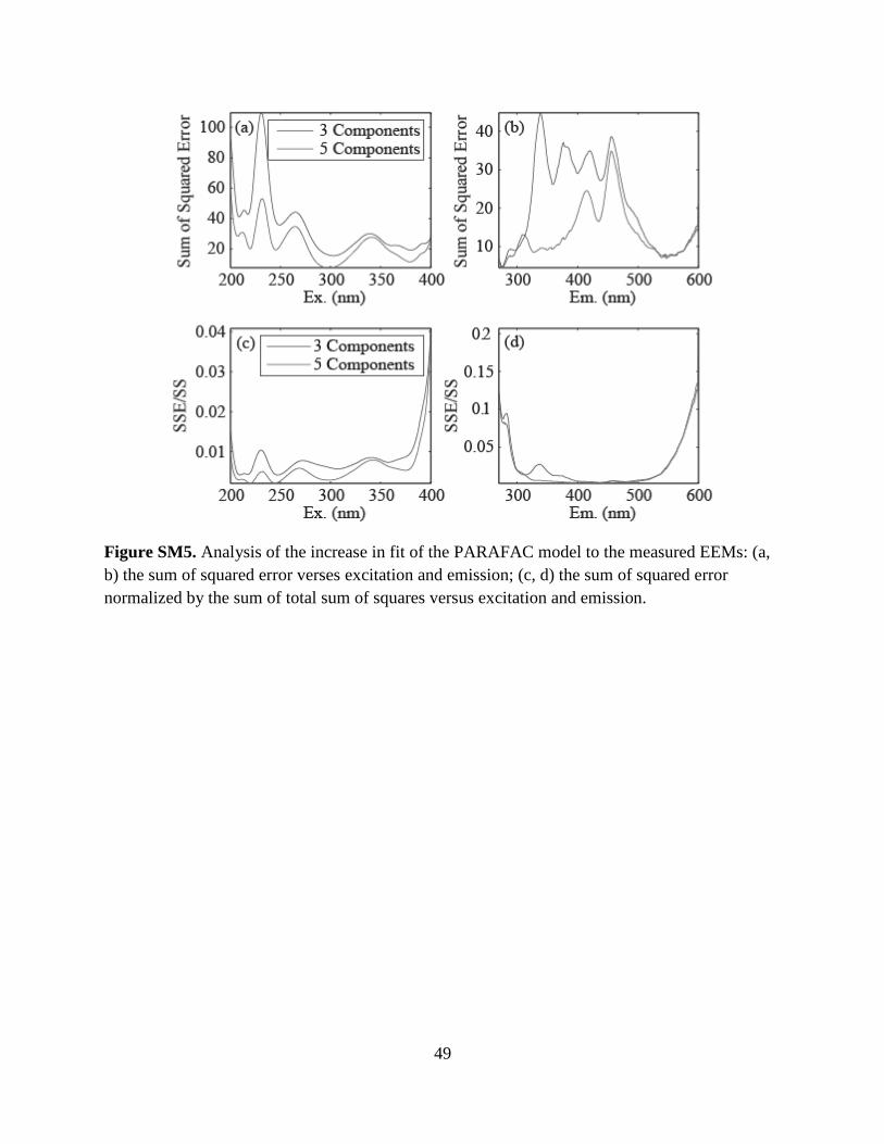
Figure SM5. Analysis of the increase in fit of the PARAFAC model to the measured EEMs: (a, b) the sum of squared error verses excitation and emission; (c,normalized by the sum of total sum of squares versus excitation and emission.

49

Analysis of the increase in fit of the PARAFAC model to the measured EEMs: (a, b) the sum of squared error verses excitation and emission; (c, d) the sum of squared error normalized by the sum of total sum of squares versus excitation and emission.

Analysis of the increase in fit of the PARAFAC model to the measured EEMs: (a, d) the sum of squared error

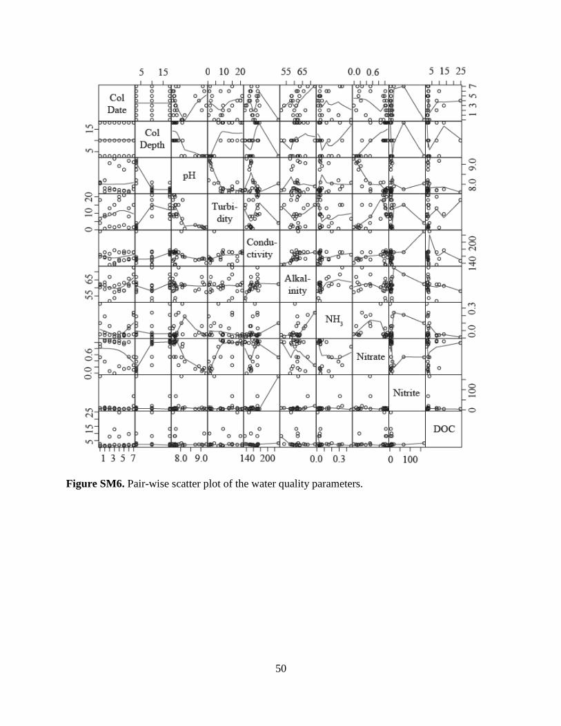
Figure SM6. Pair-wise scatter plot of the water quality parameters.

50

wise scatter plot of the water quality parameters.

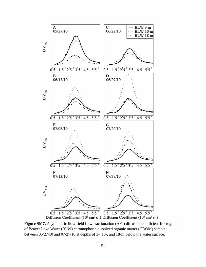
51

Figure SM7. Asymmetric flow-field flow fractionation (AF4) diffusion coefficient fractograms of Beaver Lake Water (BLW) chromophoric dissolved organic matter (CDOM) sampled between 05/27/10 and 07/27/10 at depths of 3-, 10-, and 18-m below the water surface.

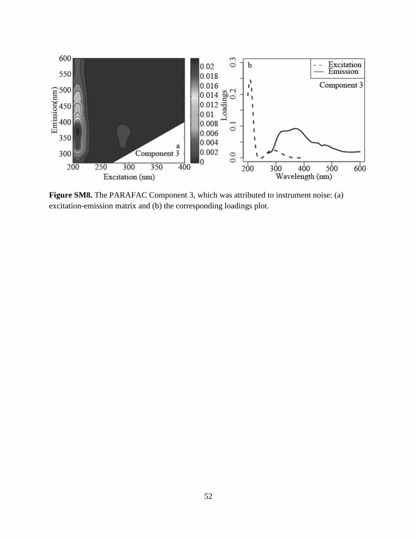
Figure SM8. The PARAFAC Component 3, which was attributed to instrument noise: (a) excitation-emission matrix and (b) the corresponding loadings plot.

52

The PARAFAC Component 3, which was attributed to instrument noise: (a) emission matrix and (b) the corresponding loadings plot.

The PARAFAC Component 3, which was attributed to instrument noise: (a)

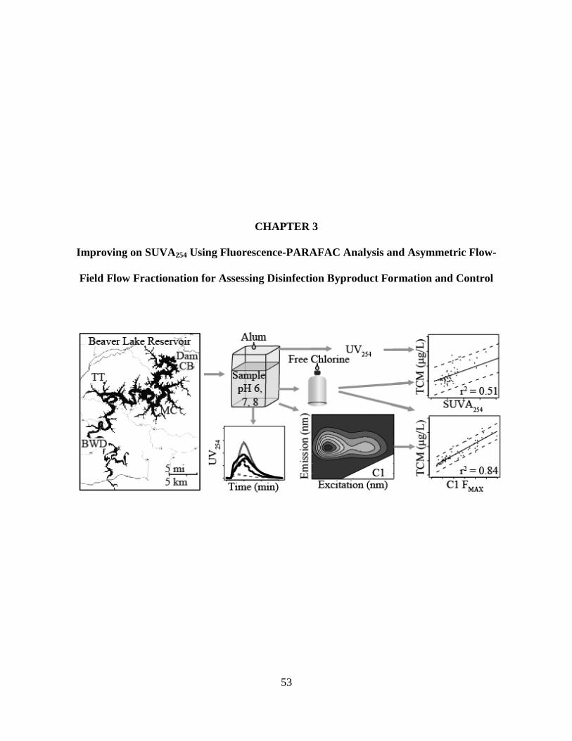
Improving on SUVA254 Using

Field Flow Fractionation for

53

CHAPTER 3

sing Fluorescence-PARAFAC Analysis and Asymmetric

ractionation for Assessing Disinfection Byproduct Formation and

symmetric Flow-

ormation and Control

54

ABSTRACT

Several challenges with disinfection byproduct (DBP) control stem from the complexity and

diversity of dissolved organic matter (DOM), which is ubiquitous in natural waters and reacts

with disinfectants to form DBPs. Fluorescence parallel factor (PARAFAC) analysis and

asymmetric flow-field flow fractionation (AF4) were used in combination with free chlorine

DBP formation potential (DBPFP) tests to study the physicochemical DOM properties and DBP

formation in raw- and alum-coagulated waters. Enhanced coagulation with alum became more

effective at removing DBP-precursors as the pH decreased from 8 to 6. AF4-UV254 fractograms

indicated enhanced coagulation at pH 6 preferentially removed larger DOM, whereas no

preferential size removal occurred at pH 8. Fluorescence-PARAFAC analysis revealed the

presence of one protein-like and three humic-like fluorophore groups; stronger linear correlations

were found between chloroform and the maximum intensity (FMAX ) of a humic-like fluorophore

(r2 = 0.84) than with SUVA254 (r2 = 0.51). This result indicated that the fluorescence-PARAFAC

approach used here was an improvement on SUVA254, i.e., fluorescence-based measurements

were stronger predictors of chloroform formation.

KEYWORDS

Enhanced coagulation; dissolved organic matter; chloroform; drinking water; pH effects

ABBREVIATIONS

AF4 (asymmetric flow-field flow fractionation); BWD (Beaver Water District); CB (Carroll

Boone Water District); DBPFP (disinfection byproduct formation potential); DBPs (disinfection

byproducts); DOC (dissolved organic carbon); DOM (dissolved organic matter); DWTPs

(drinking water treatment plants); EEMs (excitation-emission matrices); FMAX (fluorophore

maximum intensity); GFF (glass fiber filters); HDPE (high-density polyethylene); MC (Madison

55

County Regional Water District); NOM (natural organic matter); PARAFAC (parallel factor

analysis); SUVA254 (specific ultraviolet absorbance at 254 nm); TDN (total dissolved nitrogen);

THMs (trihalomethanes); TN (total nitrogen); TOC (total organic carbon); TT

(Benton/Washington Regional Public Water Authority, Two Ton); UV254 (ultraviolet absorbance

at 254 nm).

1. INTRODUCTION AND MOTIVATION

Disinfection of drinking water has been crucial in the protection of public health since the

early twentieth century, but is not without challenges. Rook (1976) reported the formation of

haloforms following chlorination of natural waters from reactions with natural organic matter

(NOM), which is ubiquitous in surface and ground waters. Trihalomethanes (THMs) are the

most abundant group of DBPs formed during chlorination and have been linked to increased

cancer risk (Cantor et al. 1998) and adverse reproductive outcomes (Nieuwenhuijsen et al. 2000).

The sum of the four THMs was regulated in drinking water under the United States

Environmental Protection Agency (USEPA) Stage 1 Disinfectants/Disinfection Byproducts Rule

with THM regulations becoming more stringent following the promulgation of the Stage 2 Rule.

Other potentially harmful DBPs (e.g. haloacetonitriles) can form upon chlorination but are

currently unregulated.

Drinking water treatment plants (DWTPs) use a two-pronged approach to curb DBPs: (1)

alter the disinfectant (e.g., switch from free chlorine to chloramines) and/or (2) remove more

NOM (e.g., enhanced coagulation). Despite this, a 1997 survey showed that 20 of 100 DWTPs

exceeded the USEPA maximum contaminant level for total THMs, 80 µg/L (Arora et al. 1997).

Many DWTPs have switched disinfectants, which can decrease formation of regulated DBPs, but

can produce unintended consequences (e.g. increased occurrence of nitrification and corrosion in

56

distribution systems (Zhang et al. 2008)). A safer but typically more expensive approach to curb

DBPs is the use of enhanced coagulation with alum or another metal salt. The dominant

coagulation mechanism depends on particle concentration, as well as coagulant dose and

speciation, which is controlled in part by the solution pH (Yang et al. 2010). DWTPs attempt to

operate enhanced coagulation with alum at the optimum pH for sweep coagulation, pH 6 to 8

(Amirtharajah 1990). The effectiveness of coagulation for DBP precursor removal is dependent

on precursor properties, and tends to be highest between pH 5 and 6 (Chow et al. 2009).

However, a fraction of NOM is typically recalcitrant to alum coagulation (Drikas et al. 2003) and

can subsequently react with chlorine to form DBPs.

NOM exists in natural waters in the milligram per liter range, and is a mixture derived

from terrestrial and aquatic sources (Rosario-Ortiz et al. 2007). NOM comprises humic

substances, carboxylic acids, carbohydrates, amino acids, and proteins and can contain aromatic

and aliphatic moieties along with hydrophilic and hydrophobic regions (Yohannes et al. 2005),

the diversity of which presents challenges for removal. Further, NOM is present in a range of

sizes, adding another level of complexity. There is limited understanding of the physicochemical

characteristics of NOM especially following processes like enhanced coagulation, which, if

augmented, may lead to improved NOM removal and reductions in DBP formation.

To predict DBP formation, specific ultraviolet absorbance (SUVA254) is routinely

correlated with DBPs (Ates et al. 2007). SUVA254 is calculated as the ratio of ultraviolet

absorbance at 254 nm (UV254) and the product of the dissolved organic carbon (DOC) and UV

cell path length. This metric requires minimal sample preparation (e.g., filtration) and commonly

available analytical equipment. Filtration removes interfering particles, and the resultant NOM

can be operationally defined as dissolved organic matter (DOM). In this work, DOM was defined

57

as the NOM that passed a 1-µm pore size glass fiber filter (GFF). While SUVA254 has been of

some value in assessing DBP formation, not all DOM is sensitive to UV light (Kitis 2001).

Further, SUVA254 cannot be used to predict DBPFP successfully in waters with low SUVA254

values (Ates et al. 2007) and strong correlations between SUVA254 and DBPs are water

dependent (Weishaar et al. 2003).

To improve DOM characterizations, fluorescence indices and excitation emission

matrices (EEMs) have been investigated. Although not all DOM components fluoresce, EEMs

provide a more detailed description of DOM than SUVA254. Fluorescence EEMs have been used

to (1) identify a water’s source (Hall et al. 2005), and (2) to reveal DOM variations by season

(Miller and McKnight 2010) and sampling depth (Pifer et al. 2011). In the past, a sample’s

fluorescence components were identified by peak picking methods (Coble et al. 1990), but the

development of parallel factor analysis (PARAFAC) for EEMs (Andersen and Bro 2003)

standardized this process. PARAFAC resolves arrays of EEMs into components, or groups of

fluorophores with common excitation-emission signatures. PARAFAC components are typically

humic-like and protein-like fluorophores (Stedmon and Bro 2008) which some evidence suggests

may correlate to formation of specific DBPs (Johnstone et al. 2009).

Due to the complexity of DOM, researchers have attempted to fractionate it chemically

(e.g. resin adsorption (Hua and Reckhow 2007)) and physically (e.g. size exclusion

chromatography (Vuorio et al. 1998)) prior to analysis. However, these techniques can produce

artifacts due to pH perturbations, sample pre-concentration, and interactions of DOM with the

stationary phase, all of which can confound inferences regarding DBP formation. Conversely,

asymmetric flow-field flow fractionation (AF4), which has been used to physically characterize

DOM in natural waters (Schimpf and Wahlund 1997; Guéguen and Cuss 2011), operates in a

58

manner that can overcome many of these limitations. AF4 separates macromolecules, colloids,

and particles between 1 nm and 100 µm in size on the basis of diffusivity (Giddings 1993). The

sample molecules elute from the channel in order of increasing size, and a continuous size

distribution, or fractogram, is produced and detected by UV254. AF4-UV254 has several benefits

over traditional physical characterization techniques, including that it requires a low sample

volume (10 mL) and minimal sample pretreatment (i.e. filtration through a GFF). As such, AF4-

UV254 fractograms can be obtained before and after jar tests, allowing estimation of the changes

in DOM size distributions.

Here, fluorescence-PARAFAC analysis and AF4-UV254 were applied to study DOM

removal by enhanced coagulation and DBP formation during chlorination. The primary

objectives were to use these physicochemical characterization techniques to (1) distinguish

spatial and temporal variation in the character and treatability of DOM, (2) identify impacts of

alum coagulation on DOM and DBP formation as a function of pH, and (3) improve on SUVA254

as a predictor of DBP formation. Lake water samples were collected from the intake structures of

four DWTPs in Northwest Arkansas between May-August, 2011. Jar tests with alum were

conducted at pH 6, 7, and 8, and were followed by DBP formation potential (DBPFP) tests with

free chlorine. AF4-UV254 fractograms were collected from raw water samples and after alum

coagulation, providing estimates of the relative amounts and sizes of DOM remaining.

Fluorescence-PARAFAC identified humic-like and protein-like DOM components and was used

to track preferential removal of these components. DBPFP tests provided a means to evaluate the

effectiveness of enhanced coagulation and to compare the strength of correlations between

SUVA254 and DBPFP with those between fluorescence-PARAFAC components and DBPFP.

59


2.1. Site description

Beaver Lake, the primary drinking water source for the approximately 500,000 residents

of Northwest Arkansas, was used as the sampling site for this study. Beaver Lake is used by four

DWTPs: Beaver Water District (BWD), Benton/Washington Regional Public Water Authority,

commonly known as Two Ton (TT), Carroll Boone Water District (CB), and Madison County

Regional Water District (MC). Beaver Lake has a surface area of 103-km2, an average depth of

18-m, and a hydraulic retention time of 1.5 years (Sen et al. 2007). Beaver Lake is located on the

White River and is fed by Richland Creek, War Eagle Creek, and Brush Creek. All four rivers

drain mostly forested or agricultural lands with increasing urbanization. Fig. S1 shows the

location of the four DWTPs on Beaver Lake.

2.2. Sample collection and handling

Water samples were collected from the four DWTPs on May 13, May 31, June 28, July

14, and August 4, 2011 as detailed in the Supplementary Data. All samples were transported to

the University of Arkansas and stored in the dark at 4°C until use.

Glassware and plastic ware were prepared as described in Pifer et al. (2011). All

chemicals used were ACS-reagent grade. Aqueous solutions were prepared using water with a

resistivity of 18.2 MΩ-cm (Milli-Q water) generated by a Milli-Q Integral 3 (Millipore) or a

Barnstead NANOpure Diamond (Thermo Scientific).


Raw water pH, alkalinity, conductivity, turbidity, total ammonia, and UV254 were

measured. Next, 600 mL aliquots of sample were filtered through GFFs as described in Pifer et

al. (2011) and total dissolved nitrogen (TDN) and dissolved organic carbon (DOC) were

60

measured using Shimadzu TOC/TN analyzers. SUVA254 was calculated by dividing UV254

(normalized by the UV cell path length in meters) by DOC in mg/L. Details on the

measurements of bromide and dissolved and particulate phosphorus are in the Supplementary

Data.

2.4. Jar Tests

For each raw water sample, 1-L aliquots were adjusted to pH 6.0, 7.0, and 8.0 using 1 N

hydrochloric acid or 1 N sodium hydroxide, and jar tests with alum (aluminum sulfate

octadecahydrate) were conducted on each pH-adjusted sample. An eight-position magnetic stir

plate with variable speed control (Challenge Technology, Springdale, AR) and rectangular

plastic jars were used for the enhanced coagulation tests. Magnetic stir bars (5-cm in length) with

ring-collared ends were used to minimize breakup of the floc. An alum dose of 60 mg/L was

used throughout to evaluate the impact of coagulation pH on DOM removal and subsequent DBP

formation, rather than determine the optimum alum dose. Alum and 2-6 mL of a 10.6 g/L sodium

carbonate solution were added simultaneously to minimize pH drift during the 30 seconds of

rapid mixing (~200 rpm). The flocculation time was 30 minutes, with a mixing speed of 40 rpm.

The samples were allowed to settle quiescently for at least 30 minutes before the supernatant was

decanted. The supernatant was filtered as described in Pifer et al. (2011), pH was measured, and

two 250-mL portions were collected in amber glass jars with screw-top lids. Raw water from

each DWTP was also filtered and stored in two 250-mL jars. One jar of each raw and alum-

coagulated water was stored in the dark at 4°C until DOC, TDN, and UV254 were measured and

AF4-UV254 fractograms and fluorescence EEMs were collected.

61

2.5. Disinfection byproducts

DBPFP was measured following Standard Methods 5710-B (Eaton et al. 2005) with

modifications. One 250-mL jar of each filtered raw water and filtered alum-coagulated water was

adjusted to pH 7.0±0.2 using a phosphate buffer and chlorinated using a stock 5,000 mg/L

sodium hypochlorite solution at doses resulting in chlorine residuals between 2.6 and 8.1 mg/L

as Cl2 after seven days in the dark at room temperature. After the seven day hold time, chlorine

residuals were measured using DPD total chlorine reagent powder pillows (Hach Company) and

a spectrophotometer (Shimadzu UV-Vis 2450). Ammonium chloride was added to 30-mL

aliquots of each sample to slow DBP formation reactions without destroying haloacetonitriles

species. The chlorine residual of the remaining 220-mL sample was quenched using sodium

sulfite and the samples were stored at 4°C in the dark until pH, DOC, TDN, and UV254 were

measured and AF4-UV254 fractograms and fluorescence EEMs were collected.

Following quenching, DBPs were immediately extracted from the 30 mL aliquots by

liquid/liquid extraction following EPA 551.1 with modifications. Pentane was used as the

extraction solvent, and 1,1,1-trichloroethane was added to the pentane as the internal standard

(Wahman 2006). Concentrations of chloroform, bromodichloromethane, dibromochloromethane,

bromoform, dichloroacetonitrile, trichloroacetonitrile, dibromoacetonitrile, and 1,1,1-trichloro-2-

propanone were measured in triplicate on a gas chromatograph (Shimadzu GC-2010) with an

electron capture detector and a J&W DB-1 column (Agilent Technologies). The column was

initially held at 32°C for one minute, and was increased by 2°C/min increments until it reached

50°C and was held for ten minutes. The oven temperature increased by 2°C/minute to 160°C and

was held constant for five minutes. A 10-point standard curve from 1 to 100 µg/L was used to

62

quantify the DBPs, and blanks and check standards were run after every twelfth injection for

quality control.

2.6. Asymmetric flow-field flow fractionation

AF4 fractograms were collected on the July 14, 2011 filtered raw and alum treated

samples at pH 6 and 8 using the instrumentation and methods described in Pifer et al. (2011)

with the following modifications. Polyethersulfone (PES) membranes with a 1,000 Da molecular

weight cut-off were used in the separation channel to achieve a stable channel pressure. Elution

time was extended to 15 minutes when necessary to capture the tail of the sample peaks, and the

rinse time was extended to 10 minutes with focus pump and tip pump flowrates of 3 mL-min-1 to

thoroughly flush the AF4-channel and minimize the height of the void peak. Phosphate-

carbonate buffer solutions at pH 6 and 8 were used as eluent to ensure that pH during

fractionation remained at the coagulation pH. The conductivity of the pH 8 eluent was modified

with sodium chloride to match that of the pH 6 eluent (470 µS cm-1). The raw water samples

were run with pH 6 and pH 8 buffers so that calculated removal percentages would reflect the

impacts of coagulation only. Duplicate samples were run to ensure consistency in DOM

separation and detector performance.

2.7. Fluorescence-PARAFAC analysis

Fluorescence EEMs were collected for each filtered raw water, alum-treated water, and

chlorinated sample (160 EEMs total). To achieve numerical stability of the PARAFAC model,

thirty-three EEMs obtained from filtered raw Beaver Lake water sampled between May 2010

and May 2011 were added to the array. After three outliers were removed, the resulting 190-

EEM dataset formed the basis for a PARAFAC model. A 5-component PARAFAC model was

obtained and validated using split halves analysis. Details of the PARAFAC modeling process

63

are provided in the Supplementary Data and complete descriptions of EEM collection, scatter

correction, and PARAFAC analyses can be found in Pifer et al. (2011).


3.1. Raw Water Parameters

Raw water parameters are summarized in Table S1. Discussion of pH, turbidity,

conductivity, alkalinity, TDN, total phosphorus, and trophic state index are contained in the

Supplementary Data. SUVA254 values varied spatially by DWTP and temporally throughout the

sampling period. At the BWD, SUVA254 was high initially (11.6-L mg-1 m-1 on 5/13/11) and

subsequently dropped to values between 2.6- and 4.9-L mg-1 m-1; at TT, SUVA254 was also high

initially (12.4-L mg-1 m-1 on 5/13/11), but was erratic thereafter with values between 3.0- and

11.1-L mg-1 m-1. In contrast, SUVA254 values at CB and MC had smaller ranges and were

between 1.4- and 5.8-L mg-1 m-1 throughout the sample period. A late April rainfall event (28-cm

of rainfall in Northwest Arkansas between April 24-26, 2011 (NOAA Satellite and Information

Service 2011)) may explain some of the variation in SUVA254, as increased runoff may have

carried large amounts of humic-like material (e.g., DOM rich in UV254 absorbing groups) to the

lake, disproportionately impacting BWD and TT before being diluted or degraded prior to

reaching the intakes at MC and CB. Interestingly, DOC varied temporally and no correlation was

found between raw water DOC and SUVA254 (r2 = 0.06), suggesting varying aromatic content (as

measured by UV254) in the Beaver Lake DOM throughout the sampling period.

3.2. AF4-UV254 Fractograms

AF4-UV254 fractograms for pH 6 and 8 samples collected on 7/14/11 are shown in

duplicate in Fig. 1 for the four sampling locations as a function of time. AF4 separates DOM

macromolecules on the basis of diffusivity, and as such samples elute with time in order of

64

increasing particle size (or decreasing diffusivity). The fractograms had a void peak at

approximately 2-minutes, and with the exception of the TT raw water samples, the void and

sample peaks were similar in height and location within each pair of duplicates, indicating the

AF4-channel was flushed sufficiently between samples and the method was reproducible. For the

TT raw water samples at a given pH, the void peak height increased from one run to the next,

possibly indicating sample carryover, however the sample peak (around 5-min elution time) was

relatively unaffected.

The AF4-UV254 fractograms in Fig. 1 demonstrated the impact of alum coagulation pH

on DOM removal. For the BWD, CB, and MC samples, the AF4-UV254 peak maxima for the raw

water DOM occurred between 4.8- and 5.6-minutes. For TT, the relatively large void peak

obscured the location and height of the AF4-UV254 DOM peak maximum. For the raw waters,

the AF4-UV254 peak heights at pH 6 were higher than those at pH 8. Alum coagulation at pH 6

resulted in average reductions between 86-91% based on AF4-UV254 peak heights for the BWD,

CB, and MC samples. In contrast, coagulation at pH 8 reduced the AF4-UV254 peak height by

28% for BWD, 36% for MC, and 43% for CB. These findings were supported by Yang et al.

(2010) who reported increased removal of UV254 as coagulation pH decreased from 8 to 6.

Coagulation also produced shifts in the time to peak maximum between the raw and alum-treated

samples, but the time-shifts were larger at pH 6 (1.8-2.3 minutes) than at pH 8 (0.5 minutes).

Given the AF4 fractograms are presented in order of increasing DOM size, this result indicated

preferential removal of larger-sized DOM at pH 6, but relatively uniform, albeit less, removal of

all DOM size fractions at pH 8.

Although AF4-UV254 fractionation provides insight into changes in the physical

properties of DOM with changes in pH, it is important to note that not all molecules absorb light

65

uniformly at 254 nm and that the fractograms presented here do not provide a complete picture

of the DOM size distribution. Future work should explore the use of other inline detectors (e.g.,

DOC) for DOM size characterizations following separation by AF4.

3.3. Fluorescence-PARAFAC Analysis

A 5-component PARAFAC model was validated for an array of 190 EEMs, consisting of

raw- and alum-treated waters from the four DWTPs. However, one component, previously

identified as fluorometer instrument noise due to its presence at similar intensity in both samples

and Millipore water blanks (Pifer et al. 2011), was ignored and, as such, a 4-component model

was used here. The excitation and emission maxima of each component were listed in Table 1

and shown as EEMs in Fig. S2. Components 1 and 4 were previously identified as a humic-like

fluorophore groups (Pifer et al. 2011). Component 2 was similar to protein-like fluorophores

reported by Dubnick et al. (2010) and Marhaba and Lippincott (2000). These protein-like

moieties contain nitrogen in their structures and as such may be of importance in the formation

of nitrogen containing DBPs. Component 3 appeared to be a combination of previously

identified humic-like fluorophores, including the C peak reported by Coble (1996).

Fig. 2 shows the fluorescence intensity data of the peak maxima (FMAX ) for each

component as a function of sampling date, DWTP, and treatment (raw water and following alum

coagulation at pH 6, 7, and 8). In general, for each sampling date and location, FMAX was highest

for raw waters and decreased following alum coagulation. Further, for the alum treated samples,

FMAX increased with increasing pH between 6 and 8, implying lowering the net negative surface

charge on the DOM by decreasing the pH enhanced DOM removal. Component 1 was the most

abundant fluorophore group of the raw- and treated-water samples, and was removed to the

greatest extent by alum coagulation. To further aid in the interpretation of these data, the relative

66

percent contributions and percent removals of component 1 relative to the total FMAX were

calculated (Table 2). The percent contribution increased with increasing coagulation pH for all

sample locations, indicating it was removed to a greater extent relative to the other fluorophore

groups as the pH decreased. Further, FMAX percent removal decreased with increasing pH at all

sampling locations (e.g., 76%, 65%, and 41% removal at pH 6, 7, and 8, respectively for the four

DWTPs together). For all components, the FMAX data were pooled and averaged for the four

DWTPs and five sampling dates and reported with their corresponding standard deviations in

Table S2. Components 2, 3, and 4 had similar contributions (13-17%) to raw water fluorescence,

but were removed to varying extents. The standard deviations of the percent removals for

components 2 and 3 were too large to permit meaningful inferences with regard to trends with

pH. Component 4 had similar percent removals and pH dependence as component 1, suggesting

these fluorophore groups were more effectively removed during coagulation at lower pH.

Overall, alum coagulation at pH 6 provided the best removal of all fluorescence-PARAFAC

components. Regardless of pH, alum coagulation appeared to preferentially remove the humic-

like components 1 and 4 compared to the protein-like component 2 and the humic-like

component 3.

3.4. Disinfection Byproducts

DBPFP was measured for chlorinated raw and alum coagulated samples. Out of the eight

DBPs in the standard curve, only chloroform, dichloroacetonitrile, bromodichloromethane, and

1,1,1-trichloro-2-propanone formed at quantifiable levels. The absence of

dibromochloromethane, bromoform, and dibromoacetonitrile was not unexpected because the

bromide concentrations in the raw water samples were low (<0.05 mg L-1). Fig. 3 shows the

concentrations of chloroform, dichloroacetonitrile, bromodichloromethane, and 1,1,1-trichloro-2-

67

propanone in units of micrograms per liter as each DBP for each sampling date, DWTP, and

treatment. Due to select large deviations in the check standards, the chloroform data from

5/31/11 was excluded from subsequent regression analyses. The chlorinated CB pH 8 sample for

7/14/11 was lost during the extraction procedure and was not included in Fig. 3 or used in

regression analyses. With these exclusions, all chloroform data used in the regression analyses

had check standards within ±13%. The other DBPs formed at concentrations less than 10 µg L-1

in the raw and treated waters, which was too low to permit meaningful regression analyses.

Although pH control of all alum treated samples was effected with sodium carbonate,

some drift occurred. The pH of each sample immediately following the decanting step of the jar

tests was indicated at the top of each bar in Fig. 3.

As expected, chloroform was the dominant DBP in all raw- and alum treated-waters and

formed in concentrations between 30 and 175 µg/L. There was temporal and spatial variability in

chloroform formation potential in the raw water samples. For example, on 5/13/11, chloroform

ranged from 58 µg/L at CB to 149 µg/L at TT; similarly, chloroform at CB ranged from 58 µg/L

on 5/13/11 to 128 µg/L on 7/14/11. These results suggest that (1) the location of the source water

intake structure within a watershed can be an important aspect of DBP control strategies, and (2)

the reactivity of precursors at a given location can shift quite rapidly. For chloroform, average

percent removals and associated standard deviations for each DWTP are shown in Table 3 as a

function of coagulation pH. The data for each DWTP and the pooled data (e.g., the four DWTPs

and five sampling dates) indicate that alum treatment decreased chloroform formation, which

was positively correlated with coagulation pH (r2=0.67). Dichloroacetonitrile formation

potentials ranged from 0.5 to 7.5 µg/L, bromodichloromethane ranged from 3.5 to 10 µg/L, and

1,1,1-trichloro-2-propanone ranged between 0.1 to 7.5 µg/L, with one extreme case of 17.3 µg/L.

68

Dichloroacetonitrile, bromodichloromethane, and 1,1,1-trichloro-2-propanone were removed to

lower extents (8-35%), and were uncorrelated with coagulation pH (Table S3). Overall, these

results indicate that decreasing coagulation pH may be a useful tool for DBP reduction in treated

Beaver Lake water where chloroform dominates the total DBP formation during chlorination.

3.5. Correlations between DBP formation and DOM properties

Linear correlations were sought between DBPFP and DOM properties such as SUVA254,

chlorine demand, and FMAX for the individual PARAFAC components. There were weak,

positive correlations (Fig. 4) between chloroform and SUVA254 (r2=0.51) and chlorine demand

(r2=0.58). Correlations between chloroform and PARAFAC FMAX components 2 and 3 were

weak (r2 < 0.40, data not shown). Stronger linear correlations were found between chloroform

and PARAFAC FMAX component 1 (r2 = 0.84, Fig. 4) and component 4 (r2 = 0.76, Fig. S3); in

these plots, linear best-fit regression lines were shown along with 95% prediction intervals. This

result indicates that the fluorescence-PARAFAC approach used here was an improvement on

SUVA254, i.e., fluorescence-based measurements were more quantitatively representative of

chloroform precursors. FMAX values from component 1 could be used to predict subsequent

formation of chloroform for the waters from the four DWTPs and treatments (raw water and

alum coagulation at pH 6, 7, and 8). This correlation suggests that humic-like fluorophores were

important chloroform precursors and was particularly strong at low FMAX values (e.g., alum

treated waters), indicating that this metric may be useful in optimizing DBP control strategies

such as enhanced coagulation. Similarly, Johnstone et al. (2009) used PARAFAC on raw- and

alum-treated waters and found multi-linear regression correlations (r2 = 0.77) between

chloroform and the combination of two other PARAFAC components (one humic-like and one

protein-like fluorophore group).

69

No correlations were found with dichloroacetonitrile, bromodichloromethane, and 1,1,1-

trichloro-2-propanone and SUVA254 (r2 < 0.26, data not shown), perhaps due to the low

concentrations of these three DBPs in the raw and treated waters. Interestingly,

dichloroacetonitrile, a nitrogen containing DBP, was uncorrelated to the protein-like Component

2 as well as the three humic-like components, suggesting that predicting formation of nitrogen

containing DBPs by fluorescence-based techniques may be challenge. Bromodichloromethane

was uncorrelated with any of the PARAFAC components (r2 < 0.21), perhaps due to the low

bromide concentrations in the source waters, which prevented bromodichloromethane formation

at levels similar to chloroform. Similarly, although 1,1,1-trichloro-2-propanone has been

identified as a chloroform precursor (Suffet et al. 1976), it was uncorrelated with the PARAFAC

components and chloroform. Studies are needed with an array of water sources (e.g., varying

bromide and DOC) and treatment types (e.g., ion exchange) to determine if the FMAX correlations

determined here were source water specific or if they could be applied broadly.

4. CONCLUSIONS

AF4-UV254 and fluorescence-PARAFAC characterizations of raw and alum coagulated

Beaver Lake water samples provided the following insights into DOM removal using enhanced

coagulation and DBPFP with free chlorine:

• Spatial and temporal variation of DOM chemical properties within Beaver Lake

impacted DBP formation.

• AF4-UV254 data indicated that DOM was of similar size throughout Beaver Lake

and that coagulation at pH 6 preferentially removed larger DOM whereas that at pH 8

removed all DOM size fractions uniformly, although to a lesser extent.

70

• Fluorescence-PARAFAC analyses identified the presence of three humic-like

fluorophore groups and one protein-like fluorophore group in Beaver Lake water.

• Humic-like PARAFAC component 1 was more strongly correlated (r2 = 0.84) to

chloroform formation potential compared to SUVA254 (r2 = 0.51) and was preferentially

removed by alum coagulation.

• AF4-UV254, fluorescence-PARAFAC, SUVA254, and DBPFP showed that alum

coagulation at pH 6 removed DOM more effectively than at pH 8.

ACKNOWLEDGEMENTS

The authors gratefully acknowledge the support of the Beaver Water District (Lowell, AR) for

running the DOC samples. Soluble reactive phosphorus was measured in J. Thad Scott’s lab at

UA. Funding for ADP was provided by UA as part of the start-up package for JLF and by the

Doctoral Academy Fellowship program (UA).

Table 1 – Maxima locations and characteristics of the fluorescence-PARAFAC components.

Component Excitation

Maxima (nm) Emission

Maxima (nm) Identification

1 238 (329) 430 Humic-like (Pifer et al. 2011)

2 231 362 Protein-like (Marhaba and Lippincott

2000; Dubnick et al. 2010)

3 344 (203, 228) 426 Humic-like (Coble 1996)

4 395 (269, 213) 471 Humic-like (Pifer et al. 2011)

Values in parentheses are secondary and tertiary Excitation maxima

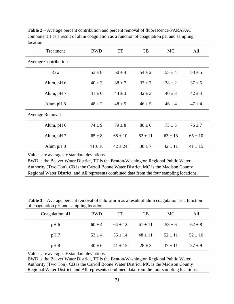
71

Table 2 – Average percent contribution and percent removal of fluorescence-PARAFAC component 1 as a result of alum coagulation as a function of coagulation pH and sampling location.

Treatment BWD TT CB MC All

Average Contribution

Raw 53 ± 8 50 ± 4 54 ± 2 55 ± 4 53 ± 5

Alum, pH 6 40 ± 3 38 ± 7 33 ± 7 38 ± 2 37 ± 5

Alum, pH 7 41 ± 6 44 ± 3 42 ± 3 40 ± 3 42 ± 4

Alum pH 8 48 ± 2 48 ± 5 46 ± 5 46 ± 4 47 ± 4

Average Removal

Alum, pH 6 74 ± 9 79 ± 8 80 ± 6 73 ± 5 76 ± 7

Alum, pH 7 65 ± 8 68 ± 10 62 ± 11 63 ± 13 65 ± 10

Alum pH 8 44 ± 18 42 ± 24 38 ± 7 42 ± 11 41 ± 15

Values are averages ± standard deviations. BWD is the Beaver Water District, TT is the Benton/Washington Regional Public Water Authority (Two Ton), CB is the Carroll Boone Water District, MC is the Madison County Regional Water District, and All represents combined data from the four sampling locations.

Table 3 – Average percent removal of chloroform as a result of alum coagulation as a function of coagulation pH and sampling location.

Coagulation pH BWD TT CB MC All

pH 6 60 ± 4 64 ± 12 61 ± 11 58 ± 6 62 ± 8

pH 7 53 ± 4 55 ± 14 48 ± 11 52 ± 11 52 ± 10

pH 8 40 ± 6 41 ± 15 28 ± 3 37 ± 11 37 ± 9

Values are averages ± standard deviations BWD is the Beaver Water District, TT is the Benton/Washington Regional Public Water Authority (Two Ton), CB is the Carroll Boone Water District, MC is the Madison County Regional Water District, and All represents combined data from the four sampling locations.

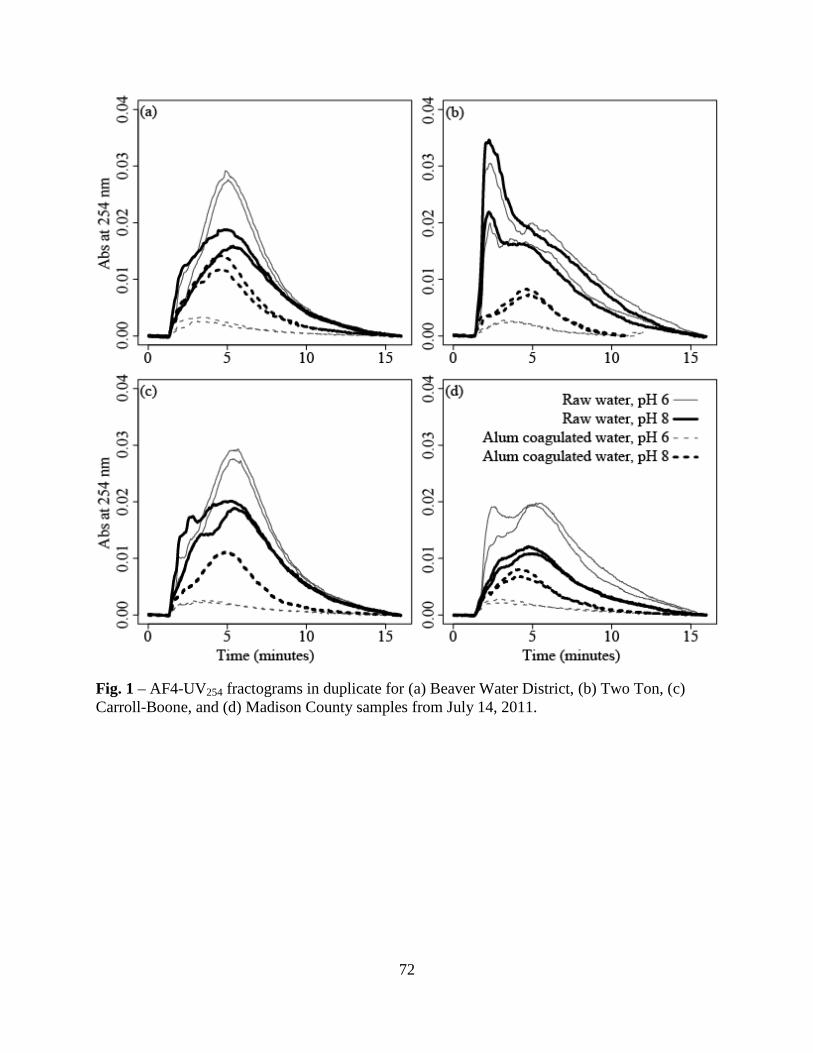
72

Fig. 1 – AF4-UV254 fractograms in duplicate for (a) Beaver Water District, (b) Two Ton, (c) Carroll-Boone, and (d) Madison County samples from July 14, 2011.

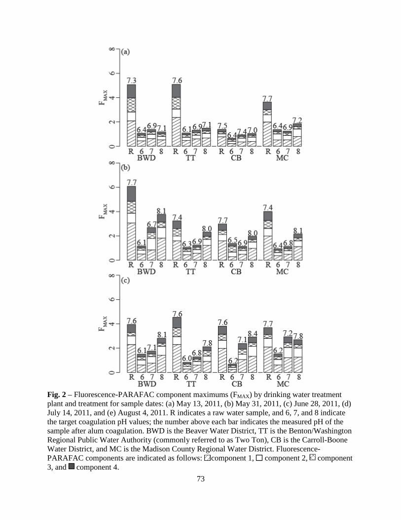
73

Fig. 2 – Fluorescence-PARAFAC component maximums (FMAX ) by drinking water treatment plant and treatment for sample dates: (a) May 13, 2011, (b) May 31, 2011, (c) June 28, 2011, (d) July 14, 2011, and (e) August 4, 2011. R indicates a raw water sample, and 6, 7, and 8 indicate the target coagulation pH values; the number above each bar indicates the measured pH of the sample after alum coagulation. BWD is the Beaver Water District, TT is the Benton/Washington Regional Public Water Authority (commonly referred to as Two Ton), CB is the Carroll-Boone Water District, and MC is the Madison County Regional Water District. Fluorescence-PARAFAC components are indicated as follows: component 1, component 2, component 3, and component 4.

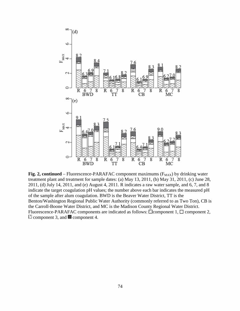
74

Fig. 2, continued – Fluorescence-PARAFAC component maximums (FMAX ) by drinking water treatment plant and treatment for sample dates: (a) May 13, 2011, (b) May 31, 2011, (c) June 28, 2011, (d) July 14, 2011, and (e) August 4, 2011. R indicates a raw water sample, and 6, 7, and 8 indicate the target coagulation pH values; the number above each bar indicates the measured pH of the sample after alum coagulation. BWD is the Beaver Water District, TT is the Benton/Washington Regional Public Water Authority (commonly referred to as Two Ton), CB is the Carroll-Boone Water District, and MC is the Madison County Regional Water District. Fluorescence-PARAFAC components are indicated as follows: component 1, component 2,

component 3, and component 4.

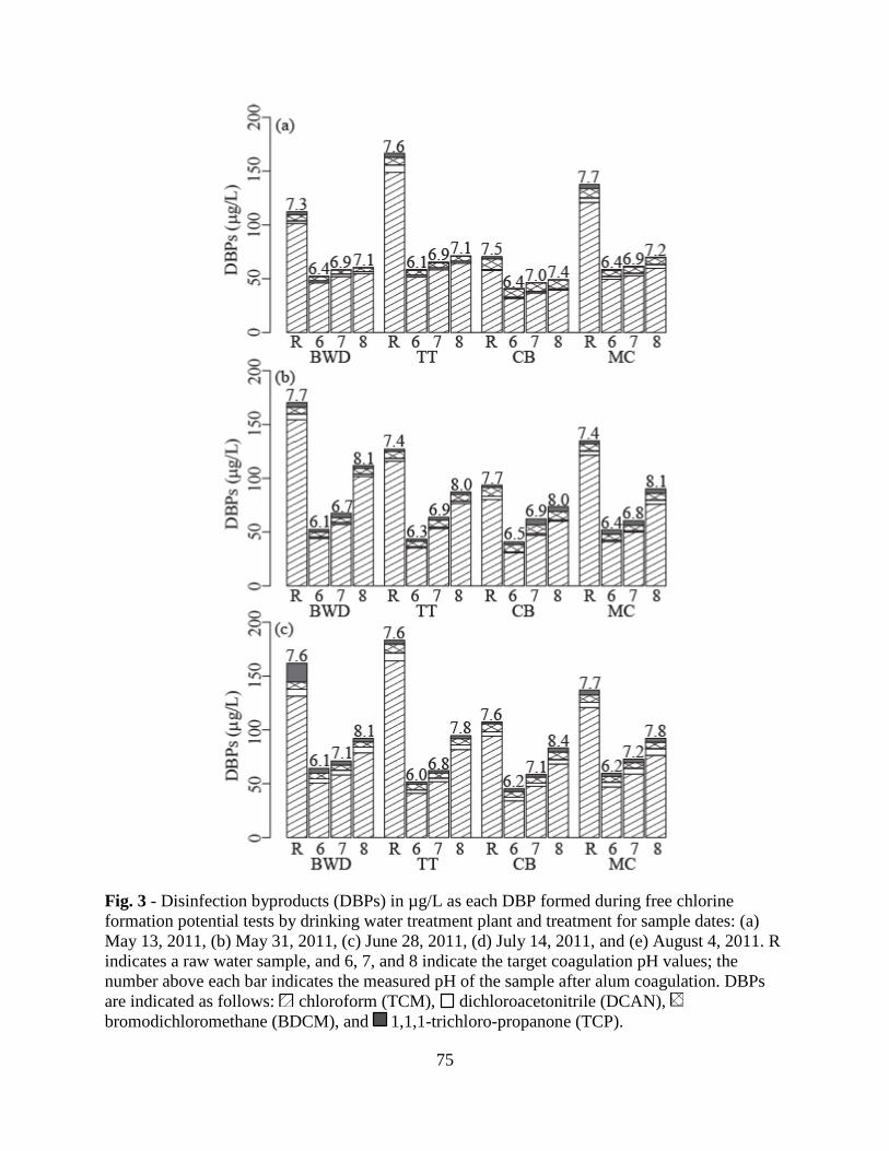
75

Fig. 3 - Disinfection byproducts (DBPs) in µg/L as each DBP formed during free chlorine formation potential tests by drinking water treatment plant and treatment for sample dates: (a) May 13, 2011, (b) May 31, 2011, (c) June 28, 2011, (d) July 14, 2011, and (e) August 4, 2011. R indicates a raw water sample, and 6, 7, and 8 indicate the target coagulation pH values; the number above each bar indicates the measured pH of the sample after alum coagulation. DBPs are indicated as follows: chloroform (TCM), dichloroacetonitrile (DCAN), bromodichloromethane (BDCM), and 1,1,1-trichloro-propanone (TCP).

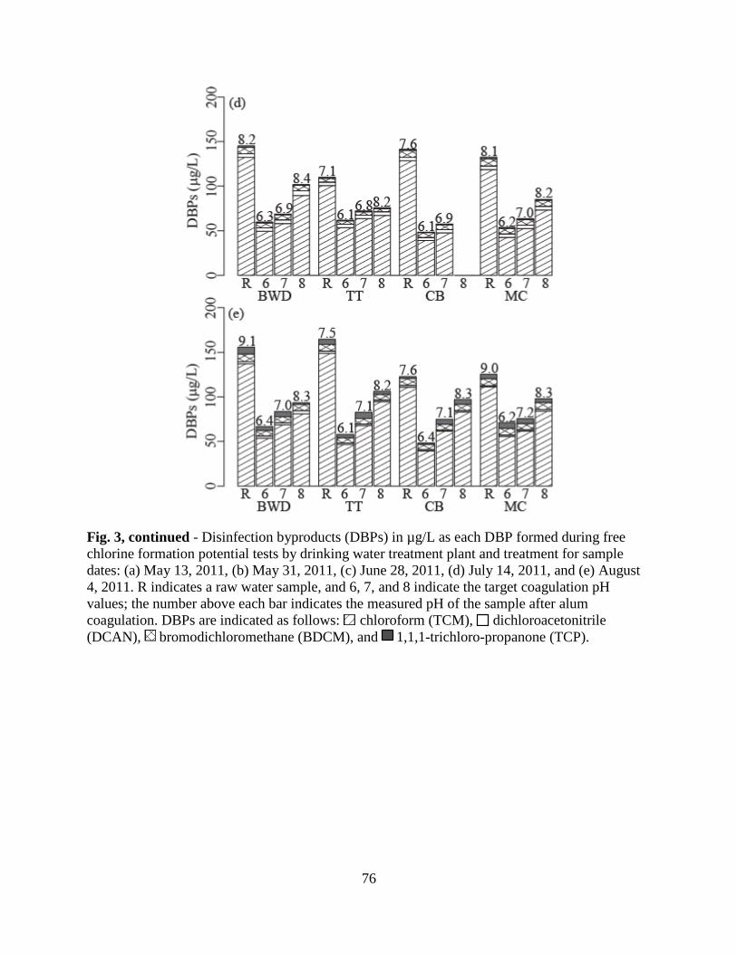
76

Fig. 3, continued - Disinfection byproducts (DBPs) in µg/L as each DBP formed during free chlorine formation potential tests by drinking water treatment plant and treatment for sample dates: (a) May 13, 2011, (b) May 31, 2011, (c) June 28, 2011, (d) July 14, 2011, and (e) August 4, 2011. R indicates a raw water sample, and 6, 7, and 8 indicate the target coagulation pH values; the number above each bar indicates the measured pH of the sample after alum coagulation. DBPs are indicated as follows: chloroform (TCM), dichloroacetonitrile (DCAN), bromodichloromethane (BDCM), and 1,1,1-trichloro-propanone (TCP).

77

Fig. 4 – Correlations between chloroform formed during the free chlorine disinfection byproduct formation potential tests and (a) chlorine demand, (b) SUVA254, and (c) FMAX for Component 1. The solid lines are the linear model fits to the experimental data. The dashed lines are the upper and lower 95% prediction intervals for the linear models.

78

5. REFERENCES

Amirtharajah, A., 1990. Coagulation: Rejuvenation for a Classical Process. Water Engineering & Management 137 (12), 25.


Arora, H., LeChevallier, M. W. and Dixon, K. L., 1997. DBP occurrence survey. Journal American Water Works Association 89 (6), 60-68.

Ates, N., Kitis, M. and Yetis, U., 2007. Formation of chlorination by-products in waters with low SUVA-correlations with SUVA and differential UV spectroscopy. Water Research 41 (18), 4139-4148.


Chow, C. W. K., van Leeuwen, J. A., Fabris, R. and Drikas, M., 2009. Optimised coagulation using aluminium sulfate for the removal of dissolved organic carbon. Desalination 245 (1-3), 120-134.



Drikas, M., Chow, C. W. K. and Cook, D., 2003. The impact of recalcitrant organic character on disinfection stability, trihalomethane formation and bacterial regrowth: An evaluation of magnetic ion exchange resin (MIEX (R)) and alum coagulation. Journal of Water Supply Research and Technology-Aqua 52 (7), 475-487.

Dubnick, A., Barker, J., Sharp, M., Wadham, J., Lis, G., Telling, J., Fitzsimons, S. and Jackson, M., 2010. Characterization of dissolved organic matter (DOM) from glacial environments using total fluorescence spectroscopy and parallel factor analysis. Annals of Glaciology 51 (56), 111-122.

Eaton, A. D., Franson, M. A. H., American Public Health Association., American Water Works Association. and Water Environment Federation., 2005. Standard methods for the examination of water & wastewater. Washington, DC, American Public Health Association.

Giddings, J. C., 1993. Field-Flow Fractionation: Analysis of Macromolecular, Colloidal, and Particulate Materials. Science 260 (5113), 1456-1465.

79

Guéguen, C. and Cuss, C. W., 2011. Characterization of aquatic dissolved organic matter by asymmetrical flow field-flow fractionation coupled to UV-Visible diode array and excitation emission matrix fluorescence. Journal of Chromatography A 1218 (27), 4188-4198.


Hua, G. and Reckhow, D. A., 2007. Characterization of Disinfection Byproduct Precursors Based on Hydrophobicity and Molecular Size. Environmental Science & Technology 41 (9), 3309-3315.


Kitis, M., Karanfil, T., Kilduff, J.E., Wigton, A., 2001. The reactivity of natural organic matter to disinfection byproducts formation and its relation to specific ultraviolet absorbance. Water Science and Technology 43 (2), 9-16.

Marhaba, T. F. and Lippincott, R. L., 2000. Application of fluorescence technique for rapid identification of DOM fractions in source waters. Journal of Environmental Engineering-Asce 126 (11), 1039-1044.

Miller, M. P. and McKnight, D. M., 2010. Comparison of seasonal changes in fluorescent dissolved organic matter among aquatic lake and stream sites in the Green Lakes Valley. J. Geophys. Res. 115, G00F12.


NOAA Satellite and Information Service (2011).


Rook, J. J., 1976. Haloforms in drinking water. Journal American Water Works Association 68 (3), 168-172.

Rosario-Ortiz, F. L., Snyder, S. A. and Suffet, I. H., 2007. Characterization of dissolved organic matter in drinking water sources impacted by multiple tributaries. Water Research 41 (18), 4115-4128.

80


Sen, S., Haggard, B., Chaubey, I., Brye, K., Costello, T. and Matlock, M., 2007. Sediment Phosphorus Release at Beaver Reservoir, Northwest Arkansas, USA, 2002–2003: A Preliminary Investigation. Water, Air, & Soil Pollution 179 (1), 67-77.


Suffet, I. H., Brenner, L. and Silver, B., 1976. Identification of 1,1,1-trichloroacetone (1,1,1-trichloropropanone) in two drinking waters: a known precursor in haloform reaction. Environmental Science & Technology 10 (13), 1273-1275.

Vuorio, E., Vahala, R., Rintala, J. and Laukkanen, R., 1998. The evaluation of drinking water treatment performed with HPSEC. Environment International 24 (5-6), 617-623.

Wahman, D. G. (2006). Cometabolism of trihalomethanes by nitrifying biofilters under drinking water treatment plant conditions. Civil, Architectural, and Environmental Engineering. Austin, The University of Texas at Austin. Ph.D: 398.

Weishaar, J. L., Aiken, G. R., Bergamaschi, B. A., Fram, M. S., Fujii, R. and Mopper, K., 2003. Evaluation of specific ultraviolet absorbance as an indicator of the chemical composition and reactivity of dissolved organic carbon. Environmental Science & Technology 37 (20), 4702-4708.

Yang, Z., Gao, B. and Yue, Q., 2010. Coagulation performance and residual aluminum speciation of Al2(SO4)3 and polyaluminum chloride (PAC) in Yellow River water treatment. Chemical Engineering Journal 165 (1), 122-132.


Zhang, Y., Griffin, A. and Edwards, M., 2008. Nitrification in premise plumbing: Role of phosphate, pH and pipe corrosion. Environmental Science & Technology 42 (12), 4280-4284.

81

APPENDIX 2

Supplementary Data for

“Improving on SUVA 254 Using Fluorescence-PARAFAC Analysis and Asymmetric Flow-

Field Flow Fractionation for Assessing Disinfection Byproduct Formation and Control”

82


1.1. Sample collection and handling.

At the BWD, the samples were collected from intake depth at the plant’s intake structure

using a 6-L Van Dorn bottle (Wildco, Model 1960-H65, Yulee, FL) and transferred to pre-rinsed

(Milli-Q water) 9-L HDPE carboys. At TT and CB, raw water samples were collected in the 9-L

HDPE carboys from taps within the DWTPs following a few minutes of flushing. At MC,

samples were collected directly from Beaver Lake next to the plant’s intake structure using the

carboys.

1.2. Water Quality Tests.

Bromide was measured in filtered samples using a Dionex DX-120 ion chromatograph

with an IonPac AS4A-SC column according to EPA 300.0. To measure particulate phosphorus

concentrations, raw water samples were filtered through acid-rinsed GFFs, which were then

digested with a 2% (w/v) persulfate solution to convert particulate phosphorus to soluble reactive

phosphorus. For dissolved phosphorus measurements, the filtrate was collected and refrigerated

until analysis. The soluble reactive phosphorus of the digested samples and filtrate was

quantified on a Trilogy fluorometer with Spreadsheet Interface Software for Trilogy software

(Turner Designs) following Standard Methods 4500-P (Eaton et al. 2005). Total phosphorus (TP)

was obtained by summing particulate phosphorus and dissolved phosphorus.

1.3. Fluorescence-PARAFAC analysis.

Fluorescence excitation-emission matrices (EEMs) were collected for a given sample in 1

nm increments between 200 and 400 nm for excitation and 270 and 600 nm for emission. The

scans were scatter-corrected using Cleanscan for MATLAB (Zepp et al. 2004). PARAFAC

modeling, using the DOM-Fluor toolbox (available for download at

83

http://www.models.life.ku.dk/algorithms), identified groups of fluorophores that made up the

EEMs. The model requires removal of outlier samples because they can bias the model. A

combination of visual identification and the function OutlierTest was used to ensure that outliers

were removed. The PARAFAC model was validated using SplitHalfAnalysis and

SplitHalfValidation.


2.1. Raw Water Parameters.

Throughout the sampling period, all four DWTPs had raw waters with slightly alkaline

pH, with a range of 7.1-8.9 and a mean of 7.7. For the first sampling date (5/13/11), BWD and

TT had high turbidity (~120 NTU) and low alkalinity (~33 mg L-1-CaCO3), likely due to 28-cm

of rainfall in Northwest Arkansas between April 24-26, 2011 (NOAA Satellite and Information

Service 2011). Turbidities decreased thereafter to values less than 20 NTU for the last three

sampling dates, with the exception of TT on 5/31/11 (60 NTU). Values of alkalinity remained

consistent throughout the sampling period, with a range of 33-56 mg L-1-CaCO3. Bromide and

ammonia concentrations were consistently below the practical quantitation limits or method

detection limits (0.05 mg L-1 as Br and 0.1 mg L-1 as N, respectively) and were not reported in

Table S1.

TDN measurements were low throughout the sampling period, with a range of 0.36-1.47

mg L-1-N, and had no consistent spatial or temporal trends. TP was highest for BWD, TT, and

MC in the 5/13/11 samples, suggesting that the runoff from the heavy rainfall event carried a

significant phosphorus load that did not make it to CB prior to sampling. TP and TDN were

uncorrelated throughout the sampling period, suggesting varying sources of these limiting

nutrients throughout Beaver Lake. Trophic state index (TSI) was calculated from TP using log-

84

linear regression equations developed by Carlson (1977). The TSI for BWD, TT, and MC was

highest on 5/13/11 (>70) and lowest on 6/28/11 (<50) where each increase in TSI major division

(e.g., from 40-50 to 50-60) represents a doubling of algal biomass. For all four DWTPs, the

average TSI based was 51, with a high for the BWD (56) and a low of CB (46), suggesting only

a modest spatial trophic gradient.

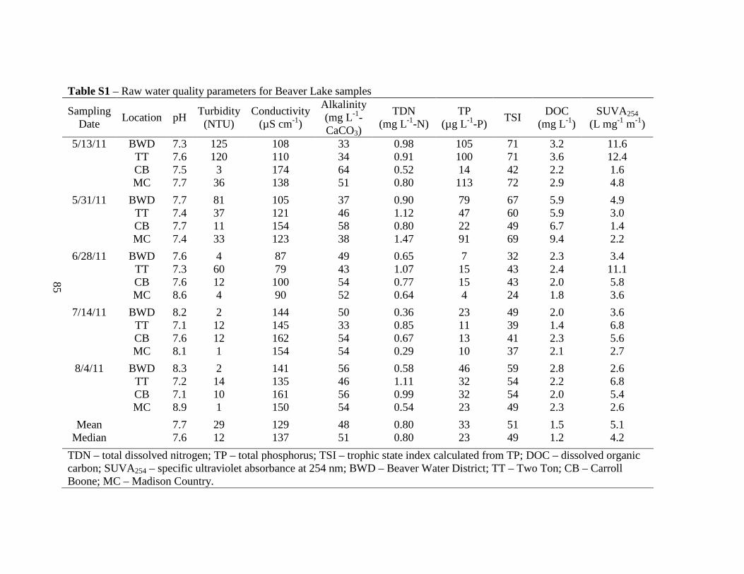
85

Table S1 – Raw water quality parameters for Beaver Lake samples

Sampling Date

Location pH Turbidity (NTU)

Conductivity (µS cm-1)

Alkalinity (mg L-1-CaCO3)

TDN (mg L-1-N)

TP (µg L-1-P)

TSI DOC

(mg L-1) SUVA254

(L mg-1 m-1)

5/13/11 BWD 7.3 125 108 33 0.98 105 71 3.2 11.6 TT 7.6 120 110 34 0.91 100 71 3.6 12.4 CB 7.5 3 174 64 0.52 14 42 2.2 1.6 MC 7.7 36 138 51 0.80 113 72 2.9 4.8

5/31/11 BWD 7.7 81 105 37 0.90 79 67 5.9 4.9 TT 7.4 37 121 46 1.12 47 60 5.9 3.0 CB 7.7 11 154 58 0.80 22 49 6.7 1.4 MC 7.4 33 123 38 1.47 91 69 9.4 2.2

6/28/11 BWD 7.6 4 87 49 0.65 7 32 2.3 3.4 TT 7.3 60 79 43 1.07 15 43 2.4 11.1 CB 7.6 12 100 54 0.77 15 43 2.0 5.8 MC 8.6 4 90 52 0.64 4 24 1.8 3.6

7/14/11 BWD 8.2 2 144 50 0.36 23 49 2.0 3.6 TT 7.1 12 145 33 0.85 11 39 1.4 6.8 CB 7.6 12 162 54 0.67 13 41 2.3 5.6 MC 8.1 1 154 54 0.29 10 37 2.1 2.7

8/4/11 BWD 8.3 2 141 56 0.58 46 59 2.8 2.6 TT 7.2 14 135 46 1.11 32 54 2.2 6.8 CB 7.1 10 161 56 0.99 32 54 2.0 5.4 MC 8.9 1 150 54 0.54 23 49 2.3 2.6

Mean 7.7 29 129 48 0.80 33 51 1.5 5.1 Median 7.6 12 137 51 0.80 23 49 1.2 4.2

TDN – total dissolved nitrogen; TP – total phosphorus; TSI – trophic state index calculated from TP; DOC – dissolved organic carbon; SUVA254 – specific ultraviolet absorbance at 254 nm; BWD – Beaver Water District; TT – Two Ton; CB – Carroll Boone; MC – Madison Country.

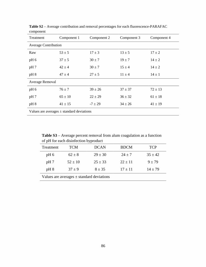
86

Table S2 – Average contribution and removal percentages for each fluorescence-PARAFAC component

Treatment Component 1 Component 2 Component 3 Component 4

Average Contribution

Raw 53 ± 5 17 ± 3 13 ± 5 17 ± 2

pH 6 37 ± 5 30 ± 7 19 ± 7 14 ± 2

pH 7 42 ± 4 30 ± 7 15 ± 4 14 ± 2

pH 8 47 ± 4 27 ± 5 11 ± 4 14 ± 1

Average Removal

pH 6 76 ± 7 39 ± 26 37 ± 37 72 ± 13

pH 7 65 ± 10 22 ± 29 36 ± 32 61 ± 18

pH 8 41 ± 15 -7 ± 29 34 ± 26 41 ± 19

Values are averages ± standard deviations

Table S3 – Average percent removal from alum coagulation as a function of pH for each disinfection byproduct

Treatment TCM DCAN BDCM TCP

pH 6 62 ± 8 29 ± 30 24 ± 7 35 ± 42

pH 7 52 ± 10 25 ± 33 22 ± 11 9 ± 79

pH 8 37 ± 9 8 ± 35 17 ± 11 14 ± 79


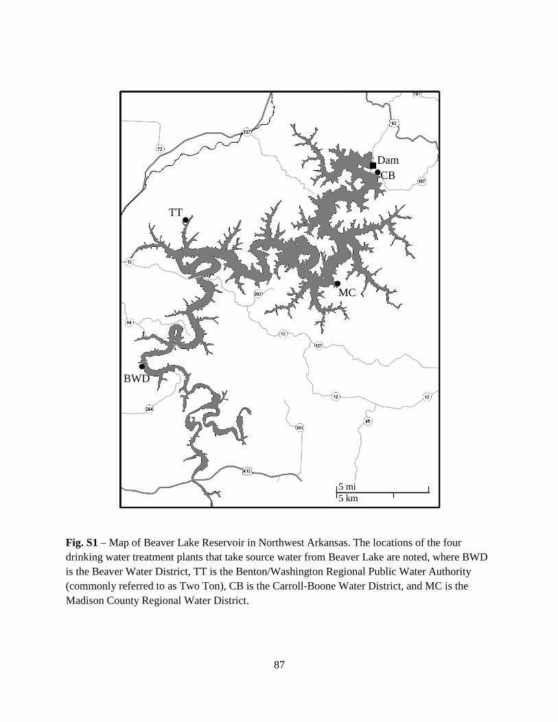
87

Fig. S1 – Map of Beaver Lake Reservoir in Northwest Arkansas. The locations of the four drinking water treatment plants that take source water from Beaver Lake are noted, where BWD is the Beaver Water District, TT is the Benton/Washington Regional Public Water Authority (commonly referred to as Two Ton), CB is the Carroll-Boone Water District, and MC is the Madison County Regional Water District.

TT

BWD

CB

MC

Dam

5 mi5 km

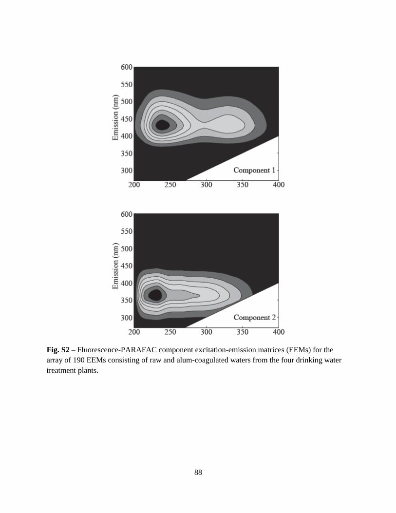
88

Fig. S2 – Fluorescence-PARAFAC component excitation-emission matrices (EEMs) for the array of 190 EEMs consisting of raw and alum-coagulated waters from the four drinking water treatment plants.

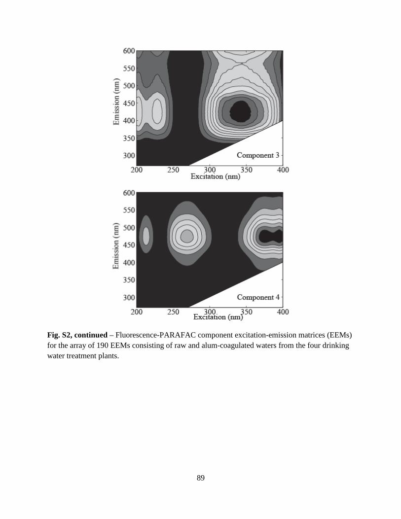
89

Fig. S2, continued – Fluorescence-PARAFAC component excitation-emission matrices (EEMs) for the array of 190 EEMs consisting of raw and alum-coagulated waters from the four drinking water treatment plants.

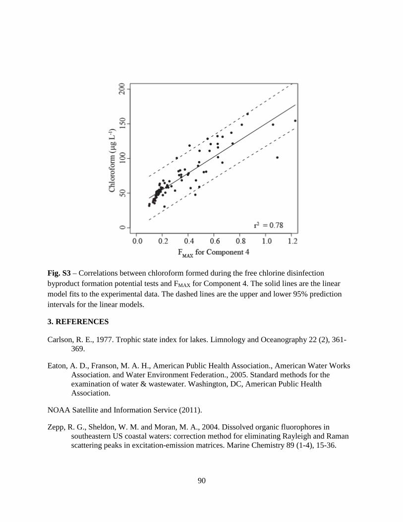
90

Fig. S3 – Correlations between chloroform formed during the free chlorine disinfection byproduct formation potential tests and FMAX for Component 4. The solid lines are the linear model fits to the experimental data. The dashed lines are the upper and lower 95% prediction intervals for the linear models.

3. REFERENCES

Carlson, R. E., 1977. Trophic state index for lakes. Limnology and Oceanography 22 (2), 361-369.


NOAA Satellite and Information Service (2011).


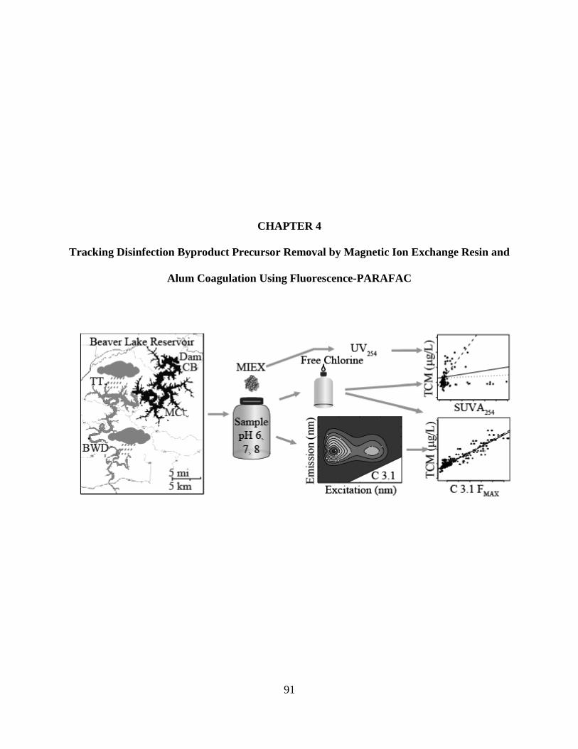
Tracking Disinfection Byproduct

Alum Coagulation

91

CHAPTER 4

yproduct Precursor Removal by Magnetic Ion Exchange

oagulation Using Fluorescence-PARAFAC

xchange Resin and

92

ABSTRACT

Removal of disinfection byproduct (DBP) precursors by magnetic ion exchange (MIEX®) resin

at pH 6, 7, and 8 was evaluated using DBP formation potential (DBPFP) tests. Chloroform was

the predominant DBP and its formation potential (FP) was reduced the greatest extent (75-82%)

by MIEX® treatment, with no apparent trends with treatment pH. Fluorescence excitation

emission matrices (EEMs) were collected from raw and MIEX®-treated samples. Parallel factor

(PARAFAC) analysis was used to decompose the EEMs into principal component fluorophore

groups, each with a maximum intensity, FMAX . This model was compared to a second model

from a previously reported alum coagulation study and to a third model resulting from the

combination of EEMs from both MIEX®- and alum-treated samples. The combined model’s

FMAX values for two humic-like fluorophore groups were more strongly correlated with

chloroform FP (r2 = 0.87 and 0.83) than specific ultraviolet absorbance at 254 nm (SUVA254,

with r2 = 0.03). The three chloroform-FMAX models showed no statistically significant differences

(p values for slopes and intercepts were greater than 0.5 and 0.1, respectively). The models also

allowed identification of 2 components that had elevated FMAX values from a heavy rainfall event

(28 cm from April 24-26, 2011), but these were uncorrelated to chloroform FP. The

corresponding SUVA254 values were also elevated and chloroform FP predictions based on them

were inaccurate. These results highlight the applicability of fluorescence-PARAFAC models to

multiple DBP precursor removal processes and suggest that FMAX may be a more selective metric

than SUVA254 for choosing and optimizing DBP precursor removal processes. In addition, the

results indicate the usefulness of FMAX values for predicting changes in DBPFP resulting from

heavy rainfall events.

93

KEYWORDS

Enhanced coagulation; anion exchange; drinking water; dissolved organic matter; chloroform;

extreme weather events

ABBREVIATIONS

BWD (Beaver Water District); CB (Carroll Boone Water District); DBP (disinfection

byproduct); DBPFP (DBP formation potential); DOC (dissolved organic carbon); DOM

(dissolved organic matter); DWTPs (drinking water treatment plants); EEMs (excitation and

emission matrices); FMAX (maximum fluorescence intensity); GFFs (glass fiber filters); HAA5

(five regulated haloacetic acids); MC (Madison County Regional Water District); MIEX®

(magnetic ion exchange); N-DBPs (nitrogen-containing DBPs ); NOM (natural organic matter);

PARAFAC (parallel factor analysis); SUVA254 (specific ultraviolet absorbance at 254 nm);

THM4 (four regulated trihalomethanes); TT (Benton-Washington Regional Public Water

Authority, commonly referred to as Two Ton); USEPA (United States Environmental Protection

Agency); UV254 (ultraviolet absorbance at 254 nm)

1. INTRODUCTION AND MOTIVATION

Disinfection byproducts (DBPs) are a concern in finished drinking waters due to their

suspected carcinogenic (Cantor et al. 1998) and teratogenic properties (Nieuwenhuijsen et al.

2000). The United States Environmental Protection Agency (USEPA) currently regulates 11

DBPs (four trihalomethanes (THM4), five of the nine haloacetic acids (HAA5), chlorite, and

bromate) in finished drinking waters under the Stage 2 Disinfection/Disinfection By-Product

Rule. Other DBPs, including nitrogen-containing DBPs (N-DBPs), are being considered for

regulation due to high toxicities relative to THM4 and HAA5. Despite nearly 40 years of DBP

94

research, DBP control remains an ongoing challenge at many drinking water treatment plants

(DWTPs).

DBPs form when drinking water disinfectants (e.g., chlorine, chloramines, ozone, etc.)

react with natural organic matter (NOM). DBP speciation and concentrations are influenced by

the disinfectant used and the quantity and characteristics of NOM. NOM is ubiquitous in natural

waters and is a complex chemical mixture consisting largely of organic carbon. NOM is derived

from both terrestrial and aquatic sources, and its physical and chemical properties can vary

temporally (Miller and McKnight 2010) and spatially (Pifer et al. 2011). Upon introduction to an

aquatic environment, NOM can be altered through biotic and abiotic processes. As such, NOM

exists as a dynamic carbon pool, which makes it difficult for DWTPs to control DBP formation

in finished drinking water.

DWTPs attempt to curb DBPs by changing their disinfectant and/or removing more DBP

precursors (i.e., NOM). Changing disinfectants can result in formation of different DBPs with

potentially higher toxicities and/or increased corrosion in the distribution system (Zhang et al.

2008; Zhang et al. 2009). As such, enhanced DBP-precursor removal has received renewed

interest in recent years.

Although enhanced coagulation is the most common method for improving NOM

removal in DWTPs, alternatives such as anion exchange have been investigated (Bolto et al.

2002). Typical ion exchange processes are operated in pressurized columns which require

prefiltration to prevent column plugging (Drikas et al. 2002). The Commonwealth Scientific &

Industrial Research Organization and Orica Australia Pty Ltd developed magnetic ion exchange

(MIEX®) resin, an anion exchange resin that has a high selectivity for NOM and can be

employed in completely mixed reactors (Drikas et al. 2002).

95

An extensive body of research exists regarding the ability of MIEX® to reduce DBP

formation potential (DBPFP) (Drikas et al. 2003; Singer et al. 2007; Jarvis et al. 2008). However,

additional research is needed to better understand the capabilities and limitations of MIEX®. In

particular, the impact of source water pH during MIEX® treatment has not been extensively

documented. Some have speculated that pH has an effect on the removal of DBP-precursors by

MIEX® due to changes in the protonation state of the acid/base NOM functional groups (Neale

and Schafer 2009), but a significant research gap regarding the optimum operating pH for

MIEX® treatment remains.

Optimization of DBP precursor removal is often based on specific ultraviolet absorbance

(SUVA254), the ultraviolet absorbance at 254 nm (UV254) in units of m-1 normalized by dissolved

organic carbon (DOC). This measurement requires filtration, and is thus taken on the portion of

NOM operationally defined as dissolved organic matter (DOM). SUVA254 can be obtained using

equipment common at DWTPs and is the most common parameter used to predict DBP

formation (Ates et al. 2007). Unfortunately, not all DOM is sensitive to UV254 (Kitis et al. 2001)

and the relationships between DBPs and SUVA254 are source water dependent (Weishaar et al.

2003) and unreliable at low SUVA254 values (Ates et al. 2007).

Fluorescence spectroscopy has become a common DOM characterization technique. It is

sensitive to aromatic and unsaturated aliphatic compounds, but is subject to quenching by

dissolved oxygen and metal ions (Senesi 1990). Fluorescence spectroscopy has the benefits of

higher sensitivity and selectivity relative to absorbance measurements. Fluorescence excitation

and emission matrices (EEMs) decomposed into fluorescent components using parallel factor

analysis (PARAFAC) have been used to identify DOM components in natural waters (Stedmon

et al. 2003) and DBP precursors in raw waters (Hua et al. 2010). Although only a fraction of

96

DOM fluoresces, DBPFP was correlated to the maximum fluorescence intensities (FMAX ) of

PARAFAC components for raw and alum treated samples from two watersheds. These

correlations were stronger than the corresponding DBPFP-SUVA254 correlations (Johnstone et al.

2009; Pifer and Fairey 2012). However, correlations between PARAFAC components and

DBPFP have not been tested after alternative treatments or across source waters.

The objectives of this study were to examine the impacts of pH on MIEX® treatment,

evaluate the effects of a heavy rainfall event on DOM properties, compare DOM removal

achieved with alum coagulation (Pifer and Fairey 2012) with that of MIEX® treatment, and test

the consistency of DBPFP-PARAFAC component correlations when applied to alum coagulated

and MIEX® treated waters. A DBP precursor surrogate that behaves consistently between

treatments would be a valuable tool to help DWTPs select and optimize treatment processes to

reduce DBPs. Raw source waters were collected monthly from May to August 2011 from four

DWTPs located on the Beaver Lake reservoir in Northwest Arkansas. These samples underwent

MIEX® treatment and alum coagulation (the alum coagulation experiments are published in Pifer

and Fairey (2012)). For the MIEX® experiments, treatment was conducted at pH 6, 7, or 8, and

the water was filtered and underwent DBPFP tests with free chlorine. Fluorescence-PARAFAC

Models 1-3 were constructed using EEMs from 1) Dataset 1, raw and MIEX® treated water, 2)

Dataset 2, raw and alum coagulated water samples (Pifer and Fairey 2012), and 3) Dataset 3, the

combination of the first two datasets. The resultant FMAX values for individual PARAFAC

components in Models 1-3 were correlated with DBPFP. These correlations were compared with

each other and to correlations between SUVA254 and DBPFP.

97

MATERIALS AND METHODS

2.1. Sampling Locations

Raw water samples (18 L each) were collected on May 13, 2011, June 28, 2011, July 14,

2011, and August 4, 2011, at the intake of four DWTPs on the Beaver Lake reservoir: Beaver

Water District (BWD), Benton-Washington Regional Public Water Authority, commonly

referred to as Two Ton (TT), Carroll Boone Water District (CB), and Madison County Regional

Water District (MC). These sampling locations were selected to assess the spatial variability of

DBP-precursors on Beaver Lake and determine the impact of this variability on MIEX treatment

and DBP formation. These raw water samples were also used in a parallel alum coagulation

study (Pifer and Fairey 2012).


All glassware, with the exception of volumetric flasks, was washed with a solution of tap

water and Alconox detergent, rinsed multiple times with Milli-Q water (18.2 MΩ-cm), and

baked for 30 minutes at 400˚C. Volumetric flasks and plastic-ware were washed with an

Alconox and tap water solution, rinsed with Milli-Q water and air-dried at room temperature. For

vacuum filtration, 1-micron glass fiber filters (GFFs) were pre-combusted (400˚C for 30 min)

and pre-rinsed (1-L Milli-Q water). Therefore, in this work DOM is operationally defined as the

portion of NOM passing a 1-micron GFF.

Raw water quality parameters, i.e., pH, alkalinity, turbidity, DOC, total dissolved

nitrogen, ammonia, and total phosphorus, were measured as part of the alum coagulation study

(Pifer and Fairey 2012), and a description of the methods can be found in its Supplementary

Data. UV254 measurements were taken on filtered samples following Standard Methods 5910-B

(Eaton et al. 2005) on the UV-Vis 2450, which was blanked with Milli-Q water before the first

98

sample and after every six samples. Thereafter, SUVA254 was calculated by dividing the UV254

absorbance by the product of the UV cell path length (0.01 m) and the DOC concentration

(mg/L).

2.3. MIEX ® Experiments

MIEX® resin (Orica Watercare, Watkins, CO) was obtained in a 5% brine solution. The

resin was prepared by decanting with glass Pasteur pipettes and rinsing with Milli-Q water until

the conductivity of the supernatant, measured with a four-cell conductivity probe (Accumet), was

less than or equal to 1 mS/cm. The MIEX® resin/Milli-Q water slurry was transferred to a 10 mL

graduated cylinder and allowed to settle for approximately 10 minutes before use. A resin dose

of 6 mL/L was chosen for all MIEX® treatments based on preliminary experiments that showed

significant DOC reduction (greater than 50%).

MIEX® experiments were conducted at pH 6, 7, and 8. To control pH, 10 mL of

phosphate buffer (68.1 g/L KH2PO4 and 11.7 g/L NaOH) was added to each 490 mL raw water

sample. The pH of the samples was further adjusted using HCl or NaOH. The samples were

transferred to 500 mL amber glass bottles, and glass pipettes were used to deliver settled resin to

the pH-buffered raw water samples. The samples were tumbled end-over-end at 45 rpm for

approximately 18 hours, a time sufficient to ensure equilibrium was achieved based on

preliminary experiments (data not shown). The samples were filtered using 1 µm GFFs before

further analyses.

2.4. Disinfection Byproduct Formation Potential Tests

DBPFP tests were conducted on 250 mL portions of raw and MIEX®-treated water

samples according to Standard Methods 5710 B with modifications. The samples were adjusted

to pH 7.0 with phosphate buffer and spiked with NaOCl solution such the chlorine residual was

99

between 3 and 7 mg/L as Cl2 after 7 days in the dark at 25˚C. Chlorine residuals were measured

using DPD total chlorine powder pillows (Hach Company) and a UV-Vis 2450

spectrophotometer (Shimadzu) calibrated at a wavelength of 552 nm with a standard curve

between 1.0 and 7.0 mg/L as Cl2. Precisely 30 mL of each chlorinated sample were taken for

DBP analysis, and the remainder was quenched by sodium sulfate and reserved for further

analyses. The 30 mL portions were quenched using ammonium chloride to preserve

haloacetonitriles, and DBPs were extracted by liquid-liquid extraction following EPA 551.1 with

modifications described in Pifer and Fairey (2012). The extraction solvent and internal standard

were combined as 0.5 mg/L 1,1,1-trichloroethane in pentane (Wahman 2006). A GC-2010 with

an electron capture detector (Shimadzu Corp.) was used to quantify DBPs. A standard curve (1,

2, 5, 10, 20, 40, 60, 80, and 100 µg/L) containing eight DBPs (chloroform,

dichlorobromomethane, dibromochloromethane, bromoform, 1,1,1-trichloro-2-propanone,

dichloroacetonitrile, trichloroacetonitrile, and dibromoacetonitrile) was run prior to the samples.

Blanks and 10 µg/L check standards were run after every twelfth injection, and all check

standards were within ± 25% of the standard concentration, considered to be acceptable based on

EPA 551.1.


Fluorescence EEMs of 200 raw and MIEX®-treated waters were collected using a dual

monochromator fluorescence detector (Agilent Technologies, Model G1321A) at excitation

wavelengths from 200 to 400 nm and emission wavelengths from 270 to 600 nm, each in 1-nm

increments. EEMs were corrected for Raleigh and Raman scattering using Cleanscan in

MATLAB (Zepp et al. 2004). Three PARAFAC models were constructed for this work using

three datasets. Model 1 was based on Dataset 1 (200 EEMs total), which contained the corrected

100

EEMs from the MIEX® experiments combined with raw Beaver Lake Water EEMs to improve

stability of the model. Model 2 was based on Dataset 2, which contained 190 EEMs from raw

and alum coagulated waters and was described in detail by Pifer and Fairey (2012). Model 3 was

based on Dataset 3, which contained the EEMs used in Models 1 and 2 (378 EEMs). PARAFAC

modeling was done in MATLAB using the DOM-Fluor toolbox (available for download at

http://www.models.life.ku.kd/algorithms). The PARAFAC algorithm decomposed the datasets

into their principal fluorophore groups (called components) and reported the signatures of these

fluorophore groups, and the FMAX values for each component in each sample. All models were

validated using the SplitHalfAnalysis and SplitHalfValidation functions. Additional details of the

PARAFAC procedure are provided elsewhere (Pifer et al. 2011; Pifer and Fairey 2012).

RESULTS AND DISCUSSION

3.1. Raw Water Parameters

Raw water parameters are presented and discussed in the Supplementary Data of Pifer

and Fairey (2012). SUVA254, often considered the most useful predictor of DBP formation,

ranged from 0.3-12.4 L mg-1 m-1, with a mean of 4.8 L mg-1 m-1. Along with turbidity, SUVA254

spiked at BWD and TT following a heavy rainfall event (28 cm from April 24-26, 2011, NOAA

Satellite and Information Service), suggesting the runoff material was rich in aromatic organics.


The EEMs in Dataset 1 resulted in a 5-component PARAFAC model, but one component

was identified as instrument noise (EEM not shown) based on a previous study (Pifer et al.

2011), leaving a 4-component model for analysis. The locations of the excitation and emission

maxima for these components are listed in Table 1 as C1.1, C1.2, C1.3, and C1.4. Based on the

location of the excitation and emission maxima, components 1.1, 1.2, and 1.4 were identified as

101

humic-like fluorophore groups (Pifer et al. 2011), and were correlated to the formation of THM4

(Pifer and Fairey 2012). Component 1.3 had an emission maximum less than 400 nm, and has

been identified as a protein-like fluorophore group (Marhaba and Lippincott 2000; Dubnick et al.

2010). Such fluorophores contain nitrogen and may play a role in the formation of N-DBPs.

Model 2, based on Dataset 2 EEMs, was also a five component model with three humic-

like components, 1 protein-like component, and 1 noise component, and component EEMs and a

description of the model was previously published (Pifer and Fairey 2012). C2.1, C2.2, C2.3 and

C2.4 were equivalent to C1.1, C1.3, C1.2, and C1.4, respectively.

A 6-component model was validated by split half analysis for Dataset 3, likely due to the

increased number of samples, and showed improvement over a valid 5-component model in

terms of sum of squared error. As before, one component was identified as instrument noise,

leaving five meaningful components. C3.1, C3.3, and C3.5 were equivalent to C1.1, C1.3, and

C1.2, respectively. The combination of FMAX from two humic-like components, C3.2 and C3.4,

were strongly correlated to FMAX from C1.4 (r2 = 0.95, data not shown). For consistency, Model

3 was used in comparisons between samples.

Figure 1 contains the FMAX values for Model 3 as a function of sampling date, location,

and treatment. The total FMAX values for the raw water samples for each DWTP and sampling

date were higher than for the corresponding treated waters. This indicated that both alum and

MIEX® resin removed portions of DOM from raw water. As in Model 2 (Pifer and Fairey 2012),

the alum-treated samples showed increasing DOM removal with decreasing pH (Fig. 1e-h).

However, there was no apparent impact of treatment pH for the MIEX®-treated samples (Fig. 1a-

d). The absence of a FMAX removal trend by pH for MIEX® treatment may indicate that the

102

portions of DOM removed by ion exchange are relatively insensitive to pH changes between 6

and 8 (Boyer et al. 2008).

FMAX for components 3.4 and 3.5 were highest in the BWD and TT samples from May

13, 2011, which suggested that they were related to the heavy rainfall event. There were no

consistent trends with sampling date or location, so Table 2 summarizes the average contribution

of each Model 3 component to the total FMAX and the average percent removal of each

component by each treatment. Component 3.1 (humic-like) was the largest contributor to each

sample’s overall fluorescence before and after treatment, and was removed by alum and MIEX®

treatment for all sample locations. Alum treatment at pH 6 performed similarly to MIEX® at pH

6, 7 and 8, but removal percentages for alum at pH 7 and 8 were lower for all locations.

Component 3.2 (humic-like) was mostly (>80%) removed by MIEX® treatment at pH 6-8 and

alum coagulation at pH 6, and to a lesser extent by alum at pH 7 and 8. Component 3.3 (protein-

like), component 3.4 (humic-like), and component 3.5 (humic-like) were more significant

contributors to the total FMAX of the samples after MIEX® treatment, indicating that MIEX®

treatment preferentially removed the other components. The resistance of components 3.4 and

3.5 were highlighted in the BWD and TT samples following the heavy rainfall event (May 13,

2011) where their raw water FMAX values were highest. Interestingly, alum treatment at pH 6, 7,

and 8 was more effective at removing components 3.4 and 3.5 than MIEX®. For the remaining

samples, the percent removals of components 3.4 and 3.5 for both alum and MIEX® were

inconsistent, as noted by the high standard deviations of these values from the mean. Negative

values for the average percent removals indicate that the treatments achieved little-to-no

removal.

103

3.3. Specific Ultraviolet Absorbance

SUVA254 and DOC values for MIEX®-treated samples are shown in Figure 2 by sampling

date, location, and treatment. SUVA254 was highest in the May 13, 2011 MIEX®-treated samples

from BWD and TT following the heavy rainfall event. The DOC values were between 0.70 and

2.15 mg L-1 as C in the MIEX®-treated samples throughout the study, so it appears that while

MIEX effectively reduced DOC in the May 13 samples, it did not remove a group of UV254-

absorbing compounds. High FMAX values for components 3.4 and 3.5 in the MIEX®-treated

samples also indicate that a specific group of compounds was resistant to MIEX® treatment.

3.4. Disinfection Byproduct Formation Potential

Of the eight DBPs screened, only three – chloroform, dichloroacetonitrile, and

bromodichloromethane – formed consistently at detectable levels (>1 µg/L) in the raw and

MIEX®-treated samples (Fig. 3). There were no spatial or temporal trends in DBPFP, so the

concentrations and percent reduction in FP with MIEX® treatment for each DBP were averaged

and listed in Table 3. Similar data for alum-treated samples were shown and discussed in Pifer

and Fairey (2012). Chloroform was the dominant DBP, and its FP was reduced to the greatest

extent by MIEX® treatment. Similar to the fluorescence-PARAFAC component data (Fig. 1 and

Table 2), no pH trends in DBP formation were apparent during MIEX® treatment. Interestingly,

bromodichloromethane concentrations increased in several instances following MIEX®

treatment, suggesting that chemicals (such as bromide ion) leached from the resin were DCBM

precursors. This was a potentially troubling result considering the bromine-substituted DBPs are

generally considered to be more toxic than fully chlorinated DBPs.

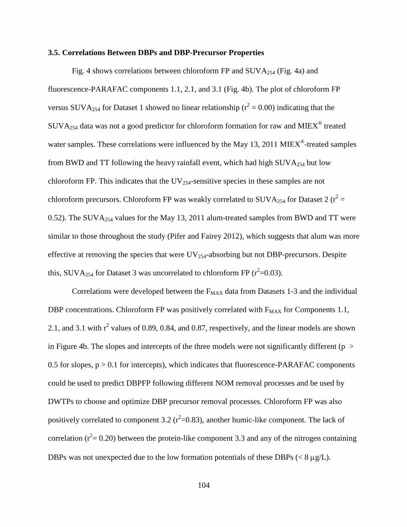
104

3.5. Correlations Between DBPs and DBP-Precursor Properties

Fig. 4 shows correlations between chloroform FP and SUVA254 (Fig. 4a) and

fluorescence-PARAFAC components 1.1, 2.1, and 3.1 (Fig. 4b). The plot of chloroform FP

versus SUVA254 for Dataset 1 showed no linear relationship (r2 = 0.00) indicating that the

SUVA254 data was not a good predictor for chloroform formation for raw and MIEX® treated

water samples. These correlations were influenced by the May 13, 2011 MIEX®-treated samples

from BWD and TT following the heavy rainfall event, which had high SUVA254 but low

chloroform FP. This indicates that the UV254-sensitive species in these samples are not

chloroform precursors. Chloroform FP was weakly correlated to SUVA254 for Dataset 2 (r2 =

0.52). The SUVA254 values for the May 13, 2011 alum-treated samples from BWD and TT were

similar to those throughout the study (Pifer and Fairey 2012), which suggests that alum was more

effective at removing the species that were UV254-absorbing but not DBP-precursors. Despite

this, SUVA254 for Dataset 3 was uncorrelated to chloroform FP (r2=0.03).

Correlations were developed between the FMAX data from Datasets 1-3 and the individual

DBP concentrations. Chloroform FP was positively correlated with FMAX for Components 1.1,

2.1, and 3.1 with r2 values of 0.89, 0.84, and 0.87, respectively, and the linear models are shown

in Figure 4b. The slopes and intercepts of the three models were not significantly different (p >

0.5 for slopes, p > 0.1 for intercepts), which indicates that fluorescence-PARAFAC components

could be used to predict DBPFP following different NOM removal processes and be used by

DWTPs to choose and optimize DBP precursor removal processes. Chloroform FP was also

positively correlated to component 3.2 (r2=0.83), another humic-like component. The lack of

correlation (r2= 0.20) between the protein-like component 3.3 and any of the nitrogen containing

DBPs was not unexpected due to the low formation potentials of these DBPs (< 8 µg/L).

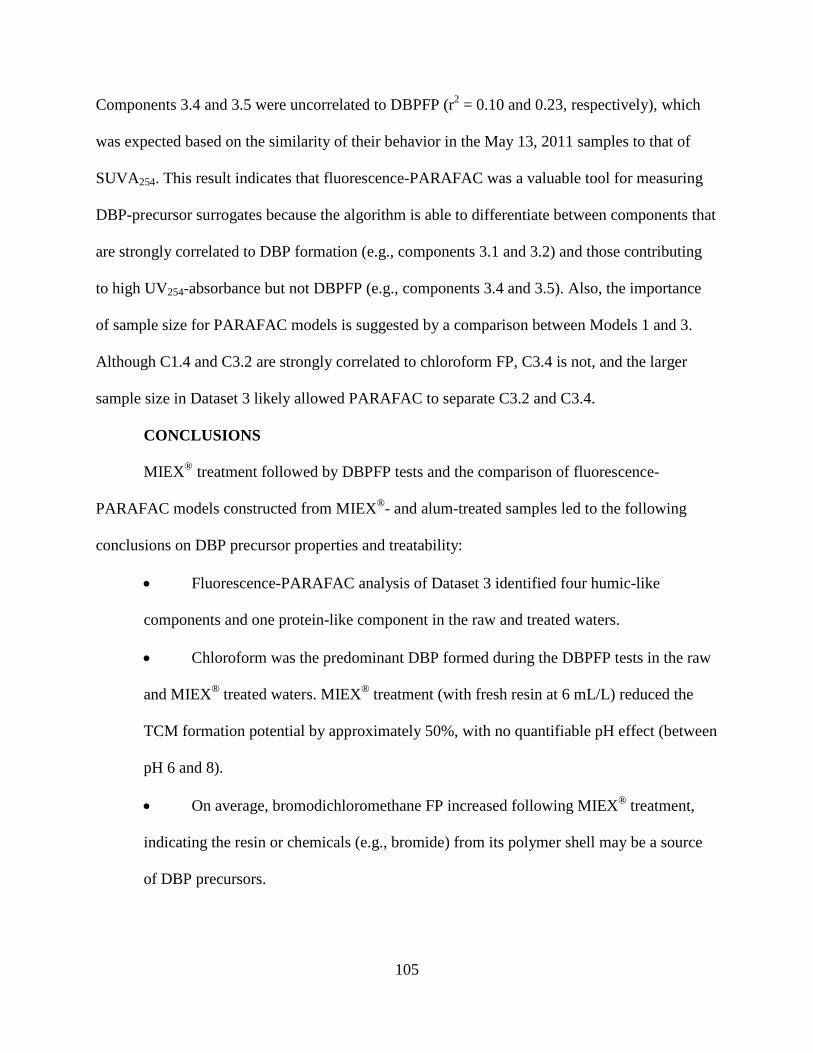
105

Components 3.4 and 3.5 were uncorrelated to DBPFP (r2 = 0.10 and 0.23, respectively), which

was expected based on the similarity of their behavior in the May 13, 2011 samples to that of

SUVA254. This result indicates that fluorescence-PARAFAC was a valuable tool for measuring

DBP-precursor surrogates because the algorithm is able to differentiate between components that

are strongly correlated to DBP formation (e.g., components 3.1 and 3.2) and those contributing

to high UV254-absorbance but not DBPFP (e.g., components 3.4 and 3.5). Also, the importance

of sample size for PARAFAC models is suggested by a comparison between Models 1 and 3.

Although C1.4 and C3.2 are strongly correlated to chloroform FP, C3.4 is not, and the larger

sample size in Dataset 3 likely allowed PARAFAC to separate C3.2 and C3.4.

CONCLUSIONS

MIEX® treatment followed by DBPFP tests and the comparison of fluorescence-

PARAFAC models constructed from MIEX®- and alum-treated samples led to the following

conclusions on DBP precursor properties and treatability:

• Fluorescence-PARAFAC analysis of Dataset 3 identified four humic-like

components and one protein-like component in the raw and treated waters.

• Chloroform was the predominant DBP formed during the DBPFP tests in the raw

and MIEX® treated waters. MIEX® treatment (with fresh resin at 6 mL/L) reduced the

TCM formation potential by approximately 50%, with no quantifiable pH effect (between

pH 6 and 8).

• On average, bromodichloromethane FP increased following MIEX® treatment,

indicating the resin or chemicals (e.g., bromide) from its polymer shell may be a source

of DBP precursors.

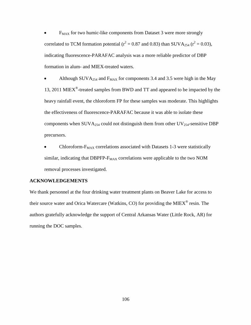
106

• FMAX for two humic-like components from Dataset 3 were more strongly

correlated to TCM formation potential (r2 = 0.87 and 0.83) than SUVA254 (r2 = 0.03),

indicating fluorescence-PARAFAC analysis was a more reliable predictor of DBP

formation in alum- and MIEX-treated waters.

• Although SUVA254 and FMAX for components 3.4 and 3.5 were high in the May

13, 2011 MIEX®-treated samples from BWD and TT and appeared to be impacted by the

heavy rainfall event, the chloroform FP for these samples was moderate. This highlights

the effectiveness of fluorescence-PARAFAC because it was able to isolate these

components when SUVA254 could not distinguish them from other UV254-sensitive DBP

precursors.

• Chloroform-FMAX correlations associated with Datasets 1-3 were statistically

similar, indicating that DBPFP-FMAX correlations were applicable to the two NOM

removal processes investigated.

ACKNOWLEDGEMENTS

We thank personnel at the four drinking water treatment plants on Beaver Lake for access to

their source water and Orica Watercare (Watkins, CO) for providing the MIEX® resin. The

authors gratefully acknowledge the support of Central Arkansas Water (Little Rock, AR) for

running the DOC samples.

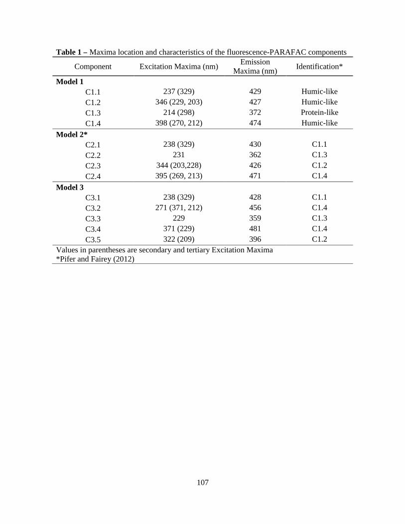
107

Table 1 – Maxima location and characteristics of the fluorescence-PARAFAC components

Component Excitation Maxima (nm) Emission

Maxima (nm) Identification*

Model 1

C1.1 237 (329) 429 Humic-like

C1.2 346 (229, 203) 427 Humic-like

C1.3 214 (298) 372 Protein-like

C1.4 398 (270, 212) 474 Humic-like

Model 2*

C2.1 238 (329) 430 C1.1

C2.2 231 362 C1.3

C2.3 344 (203,228) 426 C1.2

C2.4 395 (269, 213) 471 C1.4

Model 3

C3.1 238 (329) 428 C1.1 C3.2 271 (371, 212) 456 C1.4

C3.3 229 359 C1.3

C3.4 371 (229) 481 C1.4

C3.5 322 (209) 396 C1.2 Values in parentheses are secondary and tertiary Excitation Maxima *Pifer and Fairey (2012)

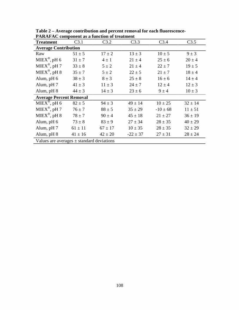
108

Table 2 – Average contribution and percent removal for each fluorescence-PARAFAC component as a function of treatment Treatment C3.1 C3.2 C3.3 C3.4 C3.5 Average Contribution Raw 51 ± 5 17 ± 2 13 ± 3 10 ± 5 9 ± 3 MIEX®, pH 6 31 ± 7 4 ± 1 21 ± 4 25 ± 6 20 ± 4 MIEX®, pH 7 33 ± 8 5 ± 2 21 ± 4 22 ± 7 19 ± 5 MIEX®, pH 8 35 ± 7 5 ± 2 22 ± 5 21 ± 7 18 ± 4 Alum, pH 6 38 ± 3 8 ± 3 25 ± 8 16 ± 6 14 ± 4 Alum, pH 7 41 ± 3 11 ± 3 24 ± 7 12 ± 4 12 ± 3 Alum, pH 8 44 ± 3 14 ± 3 23 ± 6 9 ± 4 10 ± 3 Average Percent Removal MIEX®, pH 6 82 ± 5 94 ± 3 49 ± 14 10 ± 25 32 ± 14 MIEX®, pH 7 76 ± 7 88 ± 5 35 ± 29 -10 ± 68 11 ± 51 MIEX®, pH 8 78 ± 7 90 ± 4 45 ± 18 21 ± 27 36 ± 19 Alum, pH 6 73 ± 8 83 ± 9 27 ± 34 28 ± 35 40 ± 29 Alum, pH 7 61 ± 11 67 ± 17 10 ± 35 28 ± 35 32 ± 29 Alum, pH 8 41 ± 16 42 ± 20 -22 ± 37 27 ± 31 28 ± 24


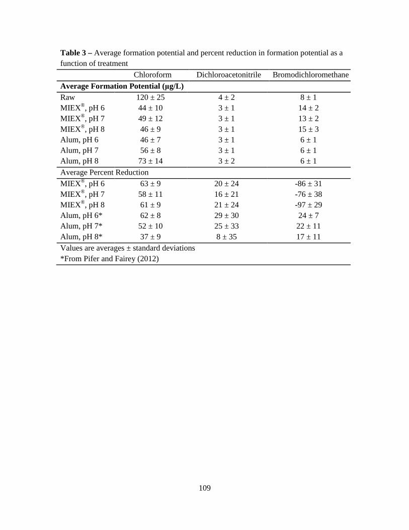
109

Table 3 – Average formation potential and percent reduction in formation potential as a function of treatment Chloroform Dichloroacetonitrile Bromodichloromethane

Average Formation Potential (µg/L) Raw 120 ± 25 4 ± 2 8 ± 1 MIEX®, pH 6 44 ± 10 3 ± 1 14 ± 2 MIEX®, pH 7 49 ± 12 3 ± 1 13 ± 2 MIEX®, pH 8 46 ± 9 3 ± 1 15 ± 3 Alum, pH 6 46 ± 7 3 ± 1 6 ± 1 Alum, pH 7 56 ± 8 3 ± 1 6 ± 1 Alum, pH 8 73 ± 14 3 ± 2 6 ± 1

Average Percent Reduction

MIEX®, pH 6 63 ± 9 20 ± 24 -86 ± 31 MIEX®, pH 7 58 ± 11 16 ± 21 -76 ± 38 MIEX®, pH 8 61 ± 9 21 ± 24 -97 ± 29 Alum, pH 6* 62 ± 8 29 ± 30 24 ± 7 Alum, pH 7* 52 ± 10 25 ± 33 22 ± 11 Alum, pH 8* 37 ± 9 8 ± 35 17 ± 11

Values are averages ± standard deviations *From Pifer and Fairey (2012)

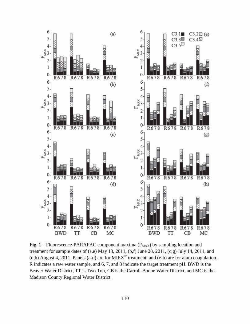
110

Fig. 1 – Fluorescence-PARAFAC component maxima (FMAX ) by sampling location and treatment for sample dates of (a,e) May 13, 2011, (b,f) June 28, 2011, (c,g) July 14, 2011, and (d,h) August 4, 2011. Panels (a-d) are for MIEX® treatment, and (e-h) are for alum coagulation. R indicates a raw water sample, and 6, 7, and 8 indicate the target treatment pH. BWD is the Beaver Water District, TT is Two Ton, CB is the Carroll-Boone Water District, and MC is the Madison County Regional Water District.

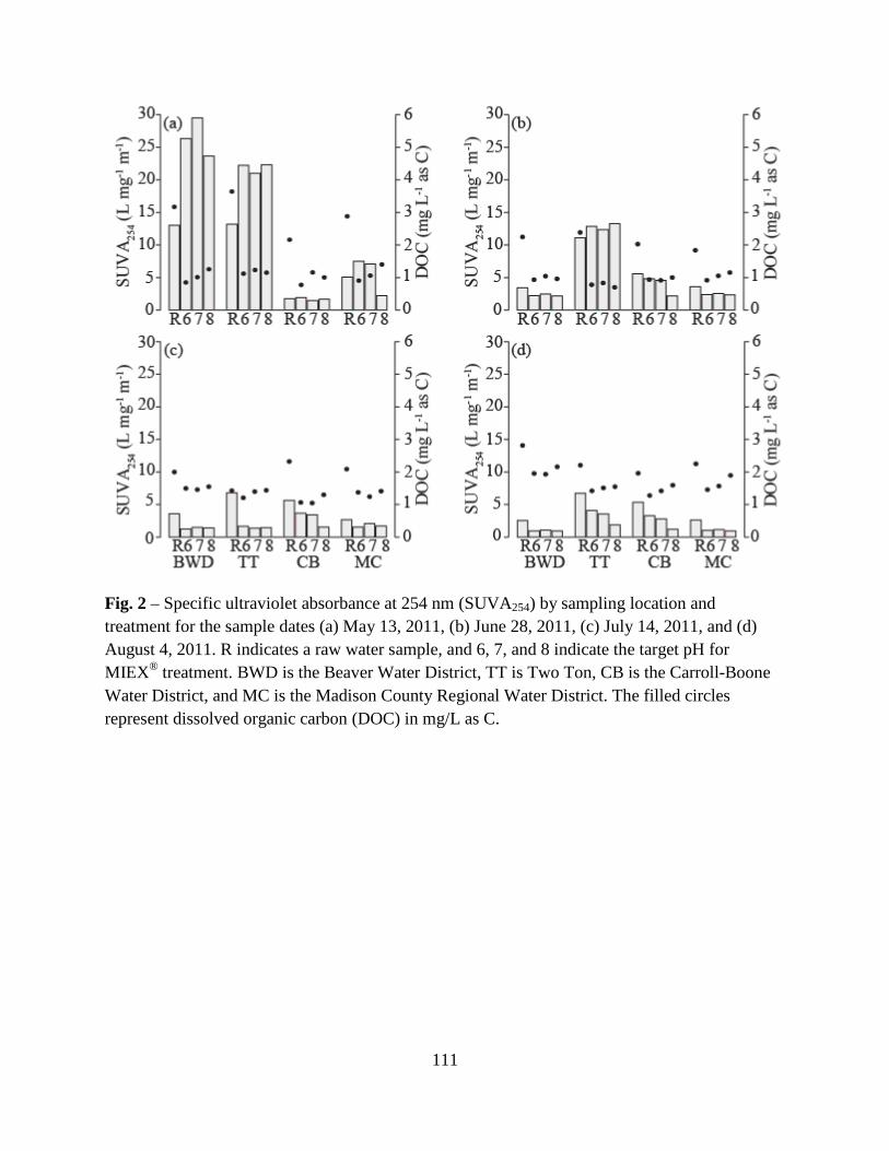
111

Fig. 2 – Specific ultraviolet absorbance at 254 nm (SUVA254) by sampling location and treatment for the sample dates (a) May 13, 2011, (b) June 28, 2011, (c) July 14, 2011, and (d) August 4, 2011. R indicates a raw water sample, and 6, 7, and 8 indicate the target pH for MIEX® treatment. BWD is the Beaver Water District, TT is Two Ton, CB is the Carroll-Boone Water District, and MC is the Madison County Regional Water District. The filled circles represent dissolved organic carbon (DOC) in mg/L as C.

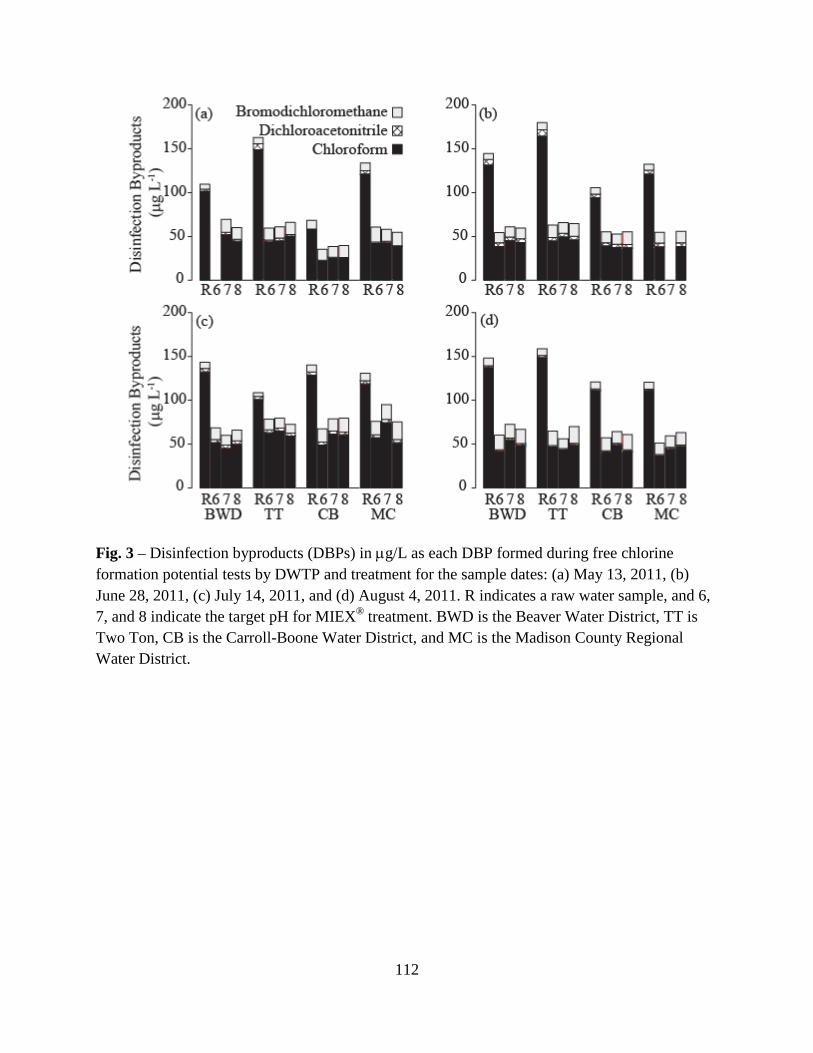
112

Fig. 3 – Disinfection byproducts (DBPs) in µg/L as each DBP formed during free chlorine formation potential tests by DWTP and treatment for the sample dates: (a) May 13, 2011, (b) June 28, 2011, (c) July 14, 2011, and (d) August 4, 2011. R indicates a raw water sample, and 6, 7, and 8 indicate the target pH for MIEX® treatment. BWD is the Beaver Water District, TT is Two Ton, CB is the Carroll-Boone Water District, and MC is the Madison County Regional Water District.

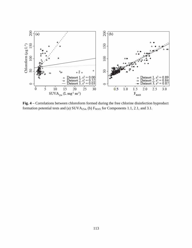
113

Fig. 4 – Correlations between chloroform formed during the free chlorine disinfection byproduct formation potential tests and (a) SUVA254, (b) FMAX for Components 1.1, 2.1, and 3.1.

114

REFERENCES

Ates, N., Kitis, M. and Yetis, U., 2007. Formation of chlorination by-products. in waters with low SUVA-correlations with SUVA and differential UV spectroscopy. Water Research 41 (18), 4139-4148.

Bolto, B., Dixon, D., Eldridge, R., King, S. and Linge, K., 2002. Removal of natural organic matter by ion exchange. Water Research 36 (20), 5057-5065.

Boyer, T. H., Singer, P. C. and Aiken, G. R., 2008. Removal of dissolved organic matter by anion exchange: Effect of dissolved organic matter properties. Environmental Science & Technology 42 (19), 7431-7437.


Drikas, M., Chow, C. W. K. and Cook, D., 2003. The impact of recalcitrant organic character on disinfection stability, trihalomethane formation and bacterial regrowth: An evaluation of magnetic ion exchange resin (MIEX (R)) and alum coagulation. Journal of Water Supply Research and Technology-Aqua 52 (7), 475-487.

Drikas, M., Morran, J. Y., Pelekani, C., Hepplewhite, C. and Bursill, D. B., 2002. Removal of natural organic matter - a fresh approach. Water Science and Technology: Water Supply 2 (1), 71-79.

Dubnick, A., Barker, J., Sharp, M., Wadham, J., Lis, G., Telling, J., Fitzsimons, S. and Jackson, M., 2010. Characterization of dissolved organic matter (DOM) from glacial environments using total fluorescence spectroscopy and parallel factor analysis. Annals of Glaciology 51 (56), 111-122.


Hua, B., Veum, K., Yang, J., Jones, J. and Deng, B. L., 2010. Parallel factor analysis of fluorescence EEM spectra to identify THM precursors in lake waters. Environmental Monitoring and Assessment 161 (1-4), 71-81.

Jarvis, P., Mergen, M., Banks, J., McIntosh, B., Parsons, S. A. and Jefferson, B., 2008. Pilot scale comparison of enhanced coagulation with magnetic resin plus coagulation systems. Environmental Science & Technology 42 (4), 1276-1282.

115


Kitis, M., Karanfil, T., Kilduff, J. E. and Wigton, A., 2001. The reactivity of natural organic matter to disinfection byproducts formation and its relation to specific ultraviolet absorbance. Water Science and Technology 43 (2), 9-16.

Marhaba, T. F. and Lippincott, R. L., 2000. Application of fluorescence technique for rapid identification of DOM fractions in source waters. Journal of Environmental Engineering-Asce 126 (11), 1039-1044.

Miller, M. P. and McKnight, D. M., 2010. Comparison of seasonal changes in fluorescent dissolved organic matter among aquatic lake and stream sites in the Green Lakes Valley. Journal of Geophysical Research-Biogeosciences 115.

Neale, P. A. and Schafer, A. I., 2009. Magnetic ion exchange: Is there potential for international development? Desalination 248 (1-3), 160-168.




Senesi, N., 1990. Molecular and quantitative aspects of the chemistry of fulvic-acid and its interactions with metal-ions and organic-chemicals. 2. The fluorescence spectroscopy approach. Analytica Chimica Acta 232 (1), 77-106.

Singer, P. C., Schneider, M., Edwards-Brandt, J. and Budd, G. C., 2007. MIEX for removal of DBP precursors: Pilot-plant findings. Journal American Water Works Association 99 (4), 128-139.

116

Stedmon, C. A., Markager, S. and Bro, R., 2003. Tracing dissolved organic matter in aquatic environments using a new approach to fluorescence spectroscopy. Marine Chemistry 82 (3-4), 239-254.


Weishaar, J. L., Aiken, G. R., Bergamaschi, B. A., Fram, M. S., Fujii, R. and Mopper, K., 2003. Evaluation of Specific Ultraviolet Absorbance as an Indicator of the Chemical Composition and Reactivity of Dissolved Organic Carbon. Environmental Science & Technology 37 (20), 4702-4708.


Zhang, Y., Griffin, A. and Edwards, M., 2008. Nitrification in premise plumbing: Role of phosphate, pH and pipe corrosion. Environmental Science & Technology 42 (12), 4280-4284.

Zhang, Y., Griffin, A., Rahman, M., Camper, A., Baribeau, H. and Edwards, M., 2009. Lead Contamination of Potable Water Due to Nitrification. Environmental Science & Technology 43 (6), 1890-1895.

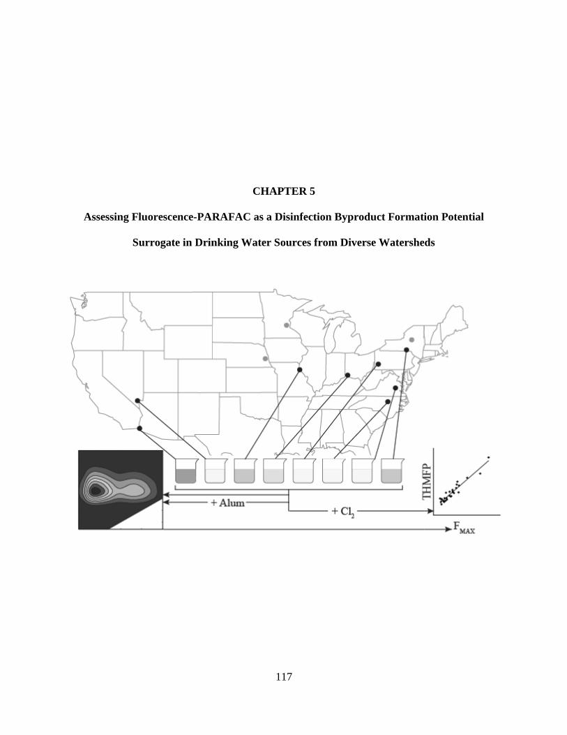
Assessing Fluorescence-PARAFAC as a

Surrogate in Drinking

117

CHAPTER 5

PARAFAC as a Disinfection Byproduct Formation

rinking Water Sources from Diverse Watersheds

ormation Potential

atersheds

118

ABSTRACT

Disinfection byproduct (DBP) control in drinking water treatment plants (DWTPs) could be

improved by the use of broadly applicable DBP surrogates to optimize treatment processes.

Fluorescence-PARAFAC components were evaluated as total trihalomethane formation potential

(TTHMFP) surrogates using source waters from eleven DWTPs within watersheds comprising 6

of the 12 dominant soil orders in the United States. Raw water samples were alum coagulated at

pH 6, 7, and 8, and underwent TTHMFP tests using free chlorine. Dissolved organic matter

(DOM) from the samples was characterized before and after alum treatment by asymmetric flow-

field flow fractionation coupled to an ultraviolet absorbance detector (AF4-UV254), specific

ultraviolet absorbance at 254 nm (SUVA254), and fluorescence-PARAFAC. AF4-UV254 showed

that alum coagulation preferentially removed the relatively large chromophoric DOM fraction at

pH 6 relative to pH 8. TTHMFP was correlated to SUVA254 and maximum fluorescence intensity

(FMAX , from PARAFAC). The TTHMFP-SUVA254 correlations were weak (r2 = 0.15, 10

DWTPs) relative to TTHMFP-FMAX correlations (r2 = 0.91 for 8 DWTPs, r2 = 0.77, 1.00 for 2

individual DWTPs), which indicated that FMAX was a stronger TTHMFP surrogate than SUVA254

and could be applied across a diverse set of water sources (10 of 11 DWTPs).

1. INTRODUCTION

Disinfection byproducts (DBPs) form from reactions between disinfectants (particularly

free chlorine) and natural organic matter (NOM) during disinfection. DBPs have been associated

with adverse health risks (Cantor et al. 1998; Nieuwenhuijsen et al. 2000), which prompted the

United States Environmental Protection Agency (USEPA) to regulate certain groups of DBPs,

such as trihalomethanes (THMs), in finished drinking water. As such, the removal of NOM, a

primary pool of DBP precursors, prior to disinfection is an important part of drinking water

119

treatment. Not all NOM reacts to form DBPs (Beggs and Summers 2011), and selective removal

of DBP precursors has been impossible in part due to difficulties in relating physicochemical

NOM properties to DBP formation (Bond et al. 2010).

NOM is a complex mixture including humic substances and proteins derived from

terrestrial and aquatic sources and therefore is subject to spatial (Stedmon et al. 2003) and

temporal (Miller and McKnight 2010) variability. An array of techniques has been employed to

characterize NOM and relate NOM properties (e.g. hydrophobicity (Kitis et al. 2002)) to DBP

formation. Size characterizations using size exclusion chromatography (Chow et al. 2008) and

asymmetric flow-field flow fractionation (AF4) (Pifer and Fairey 2012) have been used to

evaluate the effectiveness of alum coagulation for NOM removal. However, bulk NOM

characterizations are preferred by DWTPs due to the ease and low cost of obtaining them.

Metrics including total organic carbon (TOC), dissolved organic carbon (DOC, the portion of

TOC passing a 0.45 µm filter), and ultraviolet absorbance at 254 nm (UV254) have been used to

estimate NOM quantity and reactivity, and correlated to DBP formation. However, TOC and

DOC are of limited use because not all NOM is reactive. UV254 has been related to the aromatic

content of NOM (Korshin et al. 2009), and has been normalized by DOC to give specific UV254

(SUVA254), which is commonly used to optimize NOM removal processes for DBP control.

SUVA254 has successfully predicted DBP formation, but is ineffective for low SUVA254 waters

(Ates et al. 2007), such as treated waters still containing DBP precursors. Also, SUVA254-DBP

correlations are source-water dependent (Weishaar et al. 2003; Chow et al. 2008) which

decreases its value as a surrogate.

Recently, fluorescence excitation emission matrices (EEMs) have been used to

characterize NOM. Because EEMs are data-rich, statistical algorithms such as parallel factor

120

analysis (PARAFAC) have been used to resolve fluorophore groups (components) from EEMs

(Andersen and Bro 2003). Fluorescence-PARAFAC has been used to characterize NOM from

diverse sources (Murphy et al. 2006) and strong correlations between components and DBP

formation have been reported (Johnstone et al. 2009; Pifer and Fairey 2012) for individual

watersheds. Fluorescence-PARAFAC could be a significant improvement over SUVA254 as a

DBP surrogate, but its applicability to a variety of source waters remains unknown.

The objectives of this work were to (1) investigate the impacts of alum coagulation on the

physicochemical properties of NOM (e.g., AF4 was used to size NOM in raw and alum-treated

waters), (2) assess fluorescence-PARAFAC components as surrogates of DBP formation

potential (FP) in water samples collected from diverse sources, and (3) compare DBPFP-

component correlations with DBPFP-SUVA254 correlations. Raw water samples were collected

from the intakes of eleven DWTPs in the United States. Because aquatic NOM is influenced by

nearby soils (Eswaran et al. 1993; Aiken and Cotsaris 1995), the sampling locations were chosen

such that 6 of the 12 soil orders were represented. To further increase the sample variety,

samples were taken from rivers, reservoirs, and one surface water-influenced aquifer. The raw

waters were subjected to alum coagulation (at pH 6, 7, and 8) and chlorination, and fluorescence-

PARAFAC components in raw and alum-coagulated waters were correlated to DBPFP.

2. EXPERIMENTAL

2.1. Sample collection and handling.

Raw water samples were collected from the intakes of eleven DWTPs (Table 1). The

DWTPs and the principal cities they serve were: City of Binghamton Water Treatment Plant

(BNY, Binghamton, NY); Miller Treatment Plant (COH, Cincinnati, OH); Hannibal Water

Treatment Plant (HMO, Hannibal, MO); Platte River Water Treatment Plant (LNE, Lincoln,

121

NE); River Mountains Water Treatment Facility (LNV, Las Vegas, NV); Fridley Softening Plant

(MMN, Minneapolis, MN); Hays Mine Water Treatment Plant (PPA, Pittsburgh, PA); E.M.

Johnson Water Treatment Plant (RNC, Raleigh, NC); Richmond Water Treatment Plant (RVA,

Richmond, VA); Hinckley Reservoir Water Treatment Plant (UNY, Utica, NY); and Main Street

Water Treatment Facility (YAZ, Yuma, AZ). Sampling locations were chosen based on the

dominant soil order (Table 1) within each watershed (Natural Resource Conservation Service)

and the type of water source (i.e., river, lake, or groundwater under direct influence of surface

water). At each DWTP, two pre-cleaned 9-L HDPE carboys were filled headspace free with raw

water and overnight shipped on ice to the University of Arkansas and stored at 4°C in the dark

until analysis.

2.2. Glassware and reagents.

Glassware and plastic-ware were washed in a solution of Alconox detergent in tap water

and rinsed using water with a resistivity of 18.2 MΩ-cm (Milli-Q water), produced by a Milli-Q

Integral 3 (Millipore). Non-precision glassware in contact with organic solvents was baked at

400°C for 30 minutes, and other non-precision glassware was dried at 105°C. Plastic-ware was

dried at 80°C, and precision glassware was dried at room temperature. Glass fiber filters (GFFs)

with a nominal pore size of 1 micron were used for vacuum filtration. GFFs were pre-combusted

(400°C for 30 minutes) and pre-rinsed with 1 L of Milli-Q water. As such, dissolved organic

matter (DOM) and DOC were operationally defined as the organic matter or carbon,

respectively, which passed through 1 micron GFFs. All chemicals were ACS grade and all

aqueous solutions were prepared in Milli-Q water.

122

2.3. Water quality tests.

Raw water pH, alkalinity, and turbidity were measured as described by Pifer et al. (2011),

and conductivity was measured after filtration on a Malvern Zetasizer Nano ZS90. For raw and

alum-treated samples, UV254 was measured on a Shimadzu UV-Vis 2450 spectrophotometer with

a 1-cm pathlength low volume quartz cell following Standard Methods 5910-B (Eaton et al.

2005). DOC was measured on a Sievers 900 Portable TOC Analyzer with a practical

quantification limit (PQL) of 4 µg L-1. SUVA254 was calculated as UV254 (m-1) divided by DOC

(mg L-1). Bromide (PQL = 60 µg L-1) and sulfate (PQL = 160 µg L-1) were measured on a

Dionex DX-120 ion chromatograph with an IonPac AS4A-SC column following USEPA 300.0.

Aluminum (PQL = 30 µg L-1) was measured on a Spectro Genesis ICP OES following USEPA

200.7.

2.4. Jar tests.

Jar tests were conducted on each raw water sample at pH 6, 7, and 8 following Pifer and

Fairey (2012). In brief, 1-L aliquots were pH adjusted using 1 N HCl or 1 N NaOH, and were

coagulated with alum (aluminum sulfate octadecahydrate) at 60 mg L-1 on an eight-position

magnetic stir plate (Challenge Technology). To maintain the coagulation pH, 1-6 mL of 10.6 g L-

1 Na2CO3 was added simultaneously with alum. After settling, the supernatant was filtered and

stored in amber glass bottles in the dark at 4°C.

2.5. Disinfection byproducts.

DBPFP was measured following Pifer and Fairey (2012). In summary, 250 mL aliquots

of filtered raw or alum-treated water were chlorinated at pH 7.0 ± 0.2 with stock sodium

hypochlorite (5,000 mg L-1 as Cl2). Chlorine doses were chosen such that residuals were between

3.7 and 11.3 mg L-1 as Cl2 after 7 days in the dark at room temperature. After the hold time,

123

chlorine residual was measured using Hach DPD total chlorine reagent packs and the UV-Vis

spectrophotometer. Thirty mL of each chlorinated sample was quenched using ammonium

chloride, and DBPs were extracted by liquid-liquid extraction into pentane with 1,1,1-

trichloroethane as an internal standard (Wahman 2006). Concentrations of chloroform,

bromodichloromethane, dibromochloromethane, bromoform, dichloroacetonitrile,

trichloroacetonitrile, and 1,1,1-trichloro-2-propanone were measured by gas chromatography

with an electron capture detector following USEPA 551.1. Eleven-point standard curves from 0-

200 µg L-1 as each DBP were used to quantify DBPs, and blanks and check standards were

included after every twelfth injection.

2.6. Asymmetric flow-field flow fractionation.

AF4 fractograms were collected in duplicate following Pifer and Fairey (2012) using a

1,000 Da polyethersulfone membrane and an elution time of 30 minutes. Filtered raw waters

were fractionated at pH 6 and pH 8 for comparison with samples coagulated at pH 6 and 8. The

fractionation pH was controlled by the eluent, a phosphate-carbonate buffer pH-adjusted with 1

N HCl. The conductivity of the pH 8 eluent was adjusted with 1 M NaCl to match that of the pH

6 eluent (470 µS cm-1).

2.7. Fluorescence-PARAFAC analysis.

Fluorescence data was collected and analyzed following Pifer and Fairey (2012). Briefly,

fluorescence EEMs were collected using a dual monochromator fluorescence detector (Agilent

Technologies, Model G1321A) from each filtered raw and alum coagulated sample at excitation

wavelengths of 200-400 nm and emission wavelengths of 270-600 nm with 1 nm step sizes. The

EEMs were corrected for Raleigh and Raman scattering in MATLAB® with Cleanscan (Zepp et

al. 2004). The 44 EEMs were added to a dataset containing 378 EEMs from raw, alum

124

coagulated, and magnetic ion exchange- (MIEX®) treated waters from Beaver Lake in Northwest

Arkansas. A PARAFAC model for this dataset was constructed following Stedmon et al. (2008)

using the DOM-Fluor toolbox (available for download at

http://www.models.life.ku.dk/algorithms). One outlier was identified using the function

OutlierTest and was removed. The remaining 421 EEMs were resolved into one noise and five

meaningful fluorophore groups (components). The model was validated using SplitHalfAnalysis

and SplitHalfValidation, and the least squares model was chosen using RandInitAnal.


3.1. Raw water parameters.

Raw water parameters are summarized in Tables 1 and 2. The turbidity ranged from <0.1

NTU-110 NTU, with the lowest turbidity in the groundwater sample (LNE) and the 4 highest

turbidities in river samples (YAZ, COH, HMO, and BNY). Conductivity ranged from 42-1,097

µS cm-1. UNY had the lowest conductivity, likely due to an undeveloped, forested watershed

(Mohawk Valley Water Authority 2011) underlain by granite bedrock, which has been shown to

be resistant to weathering (Clow et al. 1996). YAZ and LNV had the highest conductivities,

likely due to watershed characteristics (e.g. sedimentary rock (Apodaca et al. 1996)) and human

activities (e.g. irrigation (Butler and von Guerard 1996)). The pH of the water samples ranged

from 6.9 at UNY to 8.5 at MMN. The remaining 9 samples had pH values between 7.8 and 8.2.

The alkalinity ranged from 10-232 mg L-1 as CaCO3, with the low at UNY and the high at LNE.

Similar to conductivity, sulfate ranged from 3 mg L-1 at UNY to 277 mg L-1 at YAZ. DOC

ranged from 0.69-4.07 mg L-1 as C, and SUVA254 ranged from 3.10-7.39 L mg-1-m-1. Although

DOC was lowest at PPA and highest at MMN, SUVA254 was lowest at RNC and highest at COH,

which indicated that the quantity and aromatic content of DOM varied across the sampling

125

locations. Bromide was detectable only in raw waters from LNE, LNV, PPA, and YAZ at

concentrations of 100, 60, 60, and 80 µg L-1, respectively.

3.2. Size characterization of chromophoric dissolved organic matter.

Figure 1 shows AF4 fractograms of chromophoric DOM (CDOM) with 95% confidence

intervals for each raw water at pH 6 and 8 and each coagulated water at pH 6 and 8. Each AF4

fractogram contains a void peak at approximately 2 minutes. The similar void peak heights and

times indicated that the AF4-UV254 system was sufficiently rinsed between samples and that

system performance was consistent throughout the study.

The AF4-UV254 sample peak heights for raw water CDOM varied with sample location,

with the lowest peak maxima from PPA CDOM and the highest from UNY CDOM. As reported

by Pifer and Fairey (2012), raw water samples fractionated at pH 6 had higher AF4-UV254 peak

maxima than those fractionated at pH 8. Because the mass of DOM present in each raw water

sample was the same at pH 6 and pH 8, this result indicated that CDOM characteristics were

influenced by pH. CDOM in alum coagulated waters at pH 6 and 8 resulted in lower AF4-UV254

peak maxima than the corresponding raw water, indicating CDOM removal by alum coagulation.

The reduction in AF4-UV254 peak maxima averaged 91% for coagulated pH 6 samples and 34%

for coagulated pH 8 samples. This result was similar to those of Pifer and Fairey (2012) and

Yang et al. (2010), and indicates coagulation was more effective for CDOM removal at lower

pH. However, it is important to note that CDOM removal may not represent total DOM removal,

and that coupling additional detectors (e.g. DOC) to the AF4 could allow improved estimation of

DOM removal.

In AF4, DOM is fractionated by diffusivity, and elutes from the separation channel from

highest to lowest diffusivity, or smallest to largest size. Therefore, the times to AF4-UV254 peak

126

maxima could be used to compare relative CDOM sizes, and are listed in Table S1. The peak

maxima for raw water CDOM occurred between 3.88-5.24 minutes at pH 6 and 4.08-5.37

minutes at pH 8. The CDOM remaining in alum treated waters had peak maxima between 3.25-

4.15 minutes at pH 6 and 3.61-5.21 minutes at pH 8. Raw water CDOM from COH was larger

than the other ten waters when fractionated at pH 6, whereas raw water CDOM from HMO was

largest when fractionated at pH 8. The RNC raw water CDOM was smallest at pH 6 and 8,

suggesting certain types of CDOM were more sensitive to pH. These results indicated the

importance of controlling pH during AF4 size characterizations and comparing samples

fractionated at the same pH when evaluating the impact of treatment. Alum coagulation impacted

the CDOM size distributions of many samples. Alum-treated samples at pH 6 had consistently

smaller CDOM than the corresponding raw water samples, which indicated preferential removal

of the larger CDOM fraction. Conversely, alum coagulation at pH 8 did not consistently remove

larger CDOM, and, in some cases, shifted the size distributions toward larger CDOM (LNV and

MMN samples). Overall, these results indicated that coagulation at pH 6 preferentially removed

the larger CDOM fraction and was more effective than coagulation at pH 8.

3.3. Fluorescence-PARAFAC Analysis.

A six-component PARAFAC model was constructed from the dataset consisting of 421

EEMs. Each of the six components represented a fluorophore group, and was classified by

comparing the location of the excitation and emission maxima to previously reported fluorophore

groups. One component was identified as instrument noise (Pifer et al. 2011), and was excluded

from further analysis. The remaining five components (C1-C5) and their identifications are

presented in Table 3. The PARAFAC algorithm output contains the maximum fluorescence

intensity (FMAX ) of each component, which are shown in Figure 2. Although Na2CO3 was added

127

during alum coagulation, some pH drift occurred, and the pH of each treated sample after

filtration is shown above each bar. Raw water samples from MMN, HMO, and RNC had the

highest FMAX values. These samples also had high DOC and AF4-UV254 peak maxima, but

moderate-to-low SUVA254 values (Table 2). The inconsistency of sample rankings (i.e. highest to

lowest) between the various DOM measures highlights the importance of using multiple

techniques to acquire detailed DOM characterizations and choosing appropriate metrics for

applications such as optimizing DBP control processes.

For all sampling locations, the sum of FMAX from the five components (FMAX,TOT) for raw

waters was higher than for waters coagulated at pH 6 and 7. Although coagulation at pH 8 was

effective for lowering FMAX,TOT at some locations (e.g. HMO, MMN, and RNC), little-to-no

removal was observed for LNE, LNV, PPA, RVA, and YAZ samples. The percent contribution

of each component’s FMAX to a sample’s FMAX,TOT and the percent reduction in FMAX for each

component from alum coagulation are shown in Table S2. C1 was the dominant PARAFAC

component in all raw (46-62% of FMAX,TOT) and alum-treated (24-58% of FMAX,TOT) waters, and

was removed to varying extents by alum coagulation (8-94%). On average, C1 removal

increased from 27% to 68% as coagulation pH decreased from 8 to 6, consistent with results

reported elsewhere (Pifer and Fairey 2012). C2 comprised 9 to 33% of each sample’s FMAX,TOT,

and was present in the highest levels in HMO, MMN, and RNC samples. C2 was removed by

alum coagulation at pH 6 (19-97%), but some samples showed little-to-no removal by alum

coagulation pH 7 and 8. C3 was present at low levels (1-33% of FMAX,TOT) in the majority of raw

and treated samples and was removed to varying extents by alum coagulation (0-58%). C4 was

present at low levels (7-20% of FMAX,TOT) in raw and treated samples, and was removed by alum

coagulation at pH 6 (54-91%) and pH 7 (20-82%) more so than at pH 8 (0-39%). C5 was present

128

at low levels, with highest FMAX values occurring in RNC and RVA samples. Over all sampling

locations, C5 removal varied widely (0-100%). In general, C1 and C4 were removed more

effectively than the other components at all pH values, as indicated by increasing percent

contributions of C2, C3, and C5 to FMAX,TOT following treatment.

3.4. Disinfection Byproducts.

Three THMs – chloroform, bromodichloromethane, and dibromochloromethane – were

detected at quantifiable levels (> 0.01 µM) in the chlorinated raw and alum-treated samples.

Check standards were within ±16% for chloroform, ±12% for bromodichloromethane, and ±8%

for dibromochloromethane. These checks were within EPA 551.1 requirements, i.e., 90% of

checks within ±20% and all checks within ±25%. The concentrations of each DBP are presented

in Figure 3 in micromolar units with the exception of two treated samples (HMO pH 8 and RNC

pH 7), which were lost during extraction. As in Figure 2, the final pH of each treated sample is

shown above each bar in Figure 3. For convenience, DBPFP is tabulated in Table S3 in units of

µg L-1 along with percent reductions resulting from alum treatment.

Chloroform was the dominant DBP, with concentrations ranging from 0.58-2.03 µM in

raw waters and from 0.33-1.88 µM in alum-treated waters. In general, alum coagulation removed

chloroform precursors from raw waters. Exceptions to this were treatment at pH 7 and 8 for YAZ

and pH 8 for MMN. For BNY, COH, HMO, LNV, MMN, RNC, and UNY, reduction in

chloroform FP increased with decreasing coagulation pH. Bromodichloromethane was present in

all raw (0.02-0.28 µM) and treated (0.01-0.31 µM) waters except UNY. No general trends were

observed in reduction of bromodichloromethane FP. Dibromochloromethane was present in raw

and treated waters from HMO, LNE, LNV, PPA, and YAZ at concentrations between 0.01-0.07

µM. Bromine incorporation factor (BIF) was calculated following Chang et al. (2001), and is

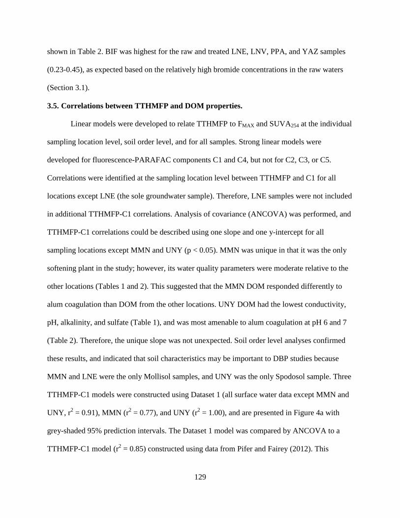
129

shown in Table 2. BIF was highest for the raw and treated LNE, LNV, PPA, and YAZ samples

(0.23-0.45), as expected based on the relatively high bromide concentrations in the raw waters

(Section 3.1).

3.5. Correlations between TTHMFP and DOM properties.

Linear models were developed to relate TTHMFP to FMAX and SUVA254 at the individual

sampling location level, soil order level, and for all samples. Strong linear models were

developed for fluorescence-PARAFAC components C1 and C4, but not for C2, C3, or C5.

Correlations were identified at the sampling location level between TTHMFP and C1 for all

locations except LNE (the sole groundwater sample). Therefore, LNE samples were not included

in additional TTHMFP-C1 correlations. Analysis of covariance (ANCOVA) was performed, and

TTHMFP-C1 correlations could be described using one slope and one y-intercept for all

sampling locations except MMN and UNY (p < 0.05). MMN was unique in that it was the only

softening plant in the study; however, its water quality parameters were moderate relative to the

other locations (Tables 1 and 2). This suggested that the MMN DOM responded differently to

alum coagulation than DOM from the other locations. UNY DOM had the lowest conductivity,

pH, alkalinity, and sulfate (Table 1), and was most amenable to alum coagulation at pH 6 and 7

(Table 2). Therefore, the unique slope was not unexpected. Soil order level analyses confirmed

these results, and indicated that soil characteristics may be important to DBP studies because

MMN and LNE were the only Mollisol samples, and UNY was the only Spodosol sample. Three

TTHMFP-C1 models were constructed using Dataset 1 (all surface water data except MMN and

UNY, r2 = 0.91), MMN (r2 = 0.77), and UNY (r2 = 1.00), and are presented in Figure 4a with

grey-shaded 95% prediction intervals. The Dataset 1 model was compared by ANCOVA to a

TTHMFP-C1 model (r2 = 0.85) constructed using data from Pifer and Fairey (2012). This

130

analysis indicated the slopes and intercepts were statistically similar (p > 0.5), suggesting C1

could be used to assess TTHMFP in a broad range of sample waters.

A similar analysis was performed for C4 with LNE excluded from the correlations.

Although the correlations between TTHMFP and C4 could be described by one slope for all

source waters, MMN required a different intercept (p < 0.01). Therefore, Figure 4b shows

TTHMFP-C4 models for Dataset 2 (all surface water data except MMN, r2 = 0.90) and MMN

itself (r2 = 0.79) with grey-shaded 95% prediction intervals. The Dataset 2 model was also

compared to TTHMFP-C4 (r2 = 0.76) data from Pifer and Fairey (2012), and the slopes were

significantly different (p < 0.001). This result indicates that despite the strong correlations

between TTHMFP and C4 observed for both datasets, C4 was not a universal predictor of

TTHMFP.

These analyses were repeated for SUVA254. Unlike C1 and C4, SUVA254 for LNE was

strongly correlated to TTHMFP (r2 = 0.94), and SUVA254 for MMN was uncorrelated to

TTHMFP. MMN was excluded from the dataset and ANCOVA was performed. TTHMFP-

SUVA254 correlations could be described with one slope and one intercept for all sampling

locations except MMN, shown as Dataset 3 (r2 = 0.15) in Figure 4c with grey-shaded 95%

prediction intervals.

Linear models were also constructed to predict formation of individual THMs using

PARAFAC components and SUVA254. Linear models for chloroform were similar to TTHMFP

models, but bromodichloromethane and dibromochloromethane did not produce meaningful

models due to smaller sample sizes and lower ranges of FPs.

These linear models indicated that although SUVA254 was an effective TTHMFP

surrogate for some sampling locations, it could not be applied to waters from a wide range of

131

sources, which confirmed the results from studies with fewer DOM sources (Weishaar et al.

2003; Pifer and Fairey 2012). TTHMFP was correlated to C1 for the 10 surface water sources,

and a single slope and intercept was applied to 8 of the 10 waters, which indicated that C1 was a

significant improvement over SUVA254 as a TTHMFP surrogate. Based on the comparisons with

data from Pifer and Fairey (2012), C1 was a more robust TTHMFP predictor than C4. The fact

that the Mollisol and Spodosol samples were outliers indicates that additional sampling should

be conducted in areas with these soil orders. It is possible that effective fluorophore-DBP

correlations could be developed for areas containing these soils, particularly Spodosols. Also,

further work is needed to determine if fluorescence-PARAFAC components would be reliable

DBPFP surrogates for groundwater sources.

4. ASSOCIATED CONTENT

Supporting Information

Contains additional information as noted, including: map of sampling locations, table of times to

AF4 peak maxima, table of the percent contributions and removals of each PARAFAC

component, and table of the DBPFP and percent reductions with treatment.

5. AUTHOR INFORMATION

Corresponding Author.

*Phone (479) 575-4023; fax (479) 575-7168; email: [email protected].

Notes

The authors declare no competing financial interest

132

ACKNOWLEDGEMENTS

This work was partially funded by grants from the Beaver Water District (Lowell, AR) and the

United States Geological Survey (Award #G11AP20066). The authors thank the participating

water utilities for their support and assistance with sample collection and shipping.

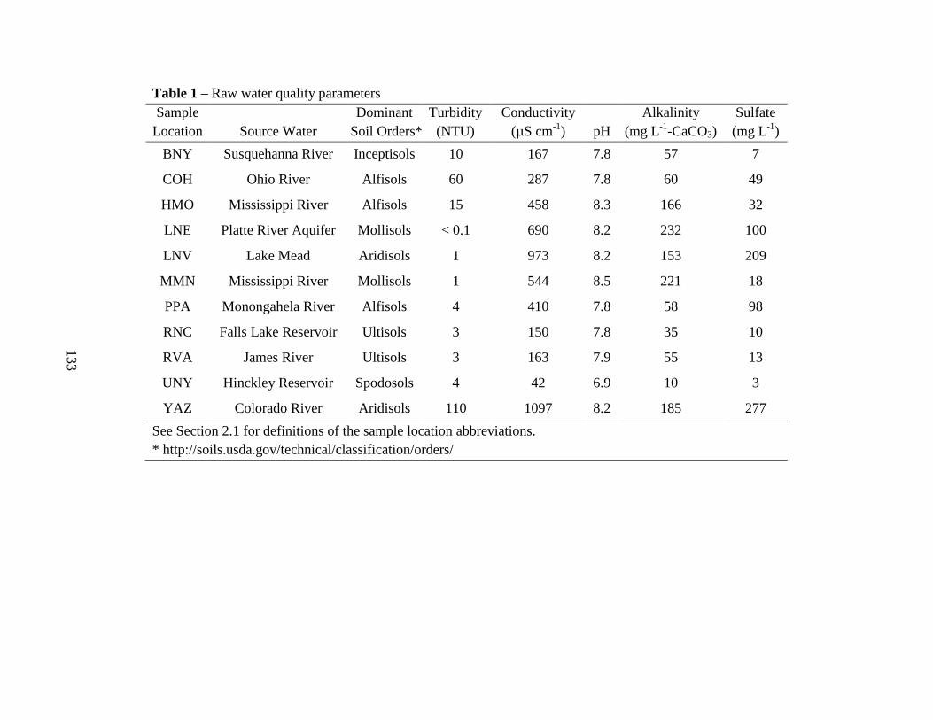
133

Table 1 – Raw water quality parameters Sample

Location Source Water Dominant

Soil Orders*Turbidity (NTU)

Conductivity (µS cm-1) pH

Alkalinity (mg L-1-CaCO3)

Sulfate (mg L-1)

BNY Susquehanna River Inceptisols 10 167 7.8 57 7

COH Ohio River Alfisols 60 287 7.8 60 49

HMO Mississippi River Alfisols 15 458 8.3 166 32

LNE Platte River Aquifer Mollisols < 0.1 690 8.2 232 100

LNV Lake Mead Aridisols 1 973 8.2 153 209

MMN Mississippi River Mollisols 1 544 8.5 221 18

PPA Monongahela River Alfisols 4 410 7.8 58 98

RNC Falls Lake Reservoir Ultisols 3 150 7.8 35 10

RVA James River Ultisols 3 163 7.9 55 13

UNY Hinckley Reservoir Spodosols 4 42 6.9 10 3

YAZ Colorado River Aridisols 110 1097 8.2 185 277

See Section 2.1 for definitions of the sample location abbreviations. * http://soils.usda.gov/technical/classification/orders/

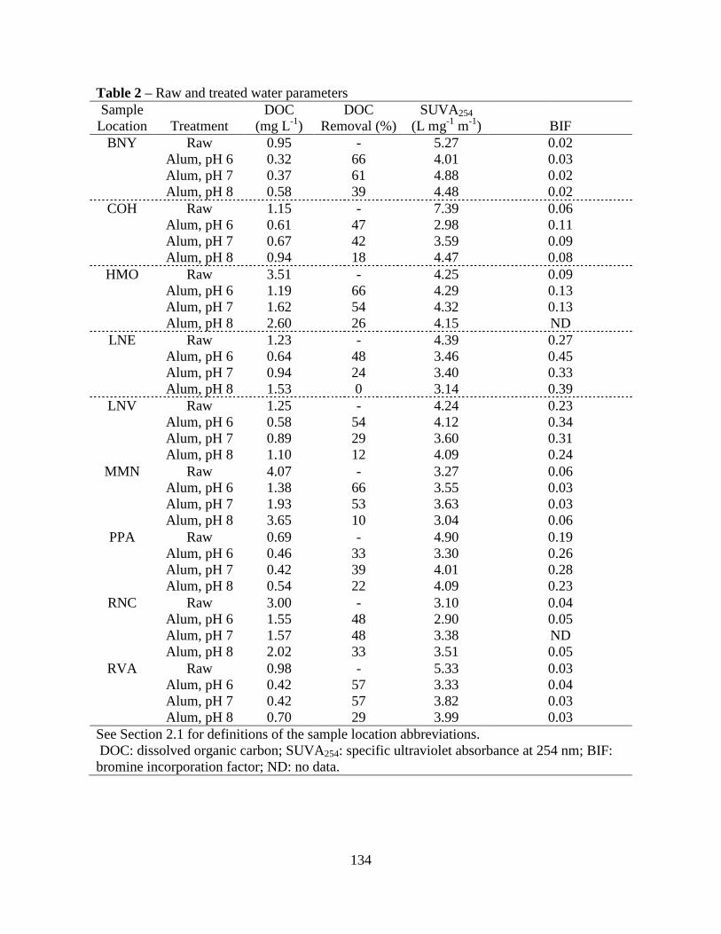
134

Table 2 – Raw and treated water parameters Sample

Location Treatment DOC

(mg L-1) DOC

Removal (%) SUVA254

(L mg-1 m-1) BIF BNY Raw 0.95 - 5.27 0.02

Alum, pH 6 0.32 66 4.01 0.03 Alum, pH 7 0.37 61 4.88 0.02 Alum, pH 8 0.58 39 4.48 0.02

COH Raw 1.15 - 7.39 0.06 Alum, pH 6 0.61 47 2.98 0.11 Alum, pH 7 0.67 42 3.59 0.09 Alum, pH 8 0.94 18 4.47 0.08

HMO Raw 3.51 - 4.25 0.09 Alum, pH 6 1.19 66 4.29 0.13 Alum, pH 7 1.62 54 4.32 0.13 Alum, pH 8 2.60 26 4.15 ND

LNE Raw 1.23 - 4.39 0.27 Alum, pH 6 0.64 48 3.46 0.45 Alum, pH 7 0.94 24 3.40 0.33 Alum, pH 8 1.53 0 3.14 0.39

LNV Raw 1.25 - 4.24 0.23 Alum, pH 6 0.58 54 4.12 0.34 Alum, pH 7 0.89 29 3.60 0.31 Alum, pH 8 1.10 12 4.09 0.24

MMN Raw 4.07 - 3.27 0.06 Alum, pH 6 1.38 66 3.55 0.03 Alum, pH 7 1.93 53 3.63 0.03 Alum, pH 8 3.65 10 3.04 0.06

PPA Raw 0.69 - 4.90 0.19 Alum, pH 6 0.46 33 3.30 0.26 Alum, pH 7 0.42 39 4.01 0.28 Alum, pH 8 0.54 22 4.09 0.23

RNC Raw 3.00 - 3.10 0.04 Alum, pH 6 1.55 48 2.90 0.05 Alum, pH 7 1.57 48 3.38 ND Alum, pH 8 2.02 33 3.51 0.05

RVA Raw 0.98 - 5.33 0.03 Alum, pH 6 0.42 57 3.33 0.04 Alum, pH 7 0.42 57 3.82 0.03 Alum, pH 8 0.70 29 3.99 0.03

See Section 2.1 for definitions of the sample location abbreviations. DOC: dissolved organic carbon; SUVA254: specific ultraviolet absorbance at 254 nm; BIF: bromine incorporation factor; ND: no data.

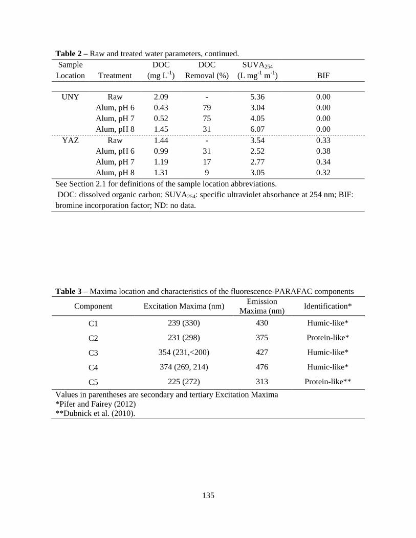
135

Table 2 – Raw and treated water parameters, continued.

Sample Location Treatment

DOC (mg L-1)

DOC Removal (%)

SUVA254 (L mg-1 m-1) BIF

UNY Raw 2.09 - 5.36 0.00 Alum, pH 6 0.43 79 3.04 0.00 Alum, pH 7 0.52 75 4.05 0.00 Alum, pH 8 1.45 31 6.07 0.00

YAZ Raw 1.44 - 3.54 0.33 Alum, pH 6 0.99 31 2.52 0.38 Alum, pH 7 1.19 17 2.77 0.34 Alum, pH 8 1.31 9 3.05 0.32

See Section 2.1 for definitions of the sample location abbreviations. DOC: dissolved organic carbon; SUVA254: specific ultraviolet absorbance at 254 nm; BIF: bromine incorporation factor; ND: no data.

Table 3 – Maxima location and characteristics of the fluorescence-PARAFAC components

Component Excitation Maxima (nm) Emission

Maxima (nm) Identification*

C1 239 (330) 430 Humic-like*

C2 231 (298) 375 Protein-like*

C3 354 (231,<200) 427 Humic-like*

C4 374 (269, 214) 476 Humic-like*

C5 225 (272) 313 Protein-like**

Values in parentheses are secondary and tertiary Excitation Maxima *Pifer and Fairey (2012) **Dubnick et al. (2010).

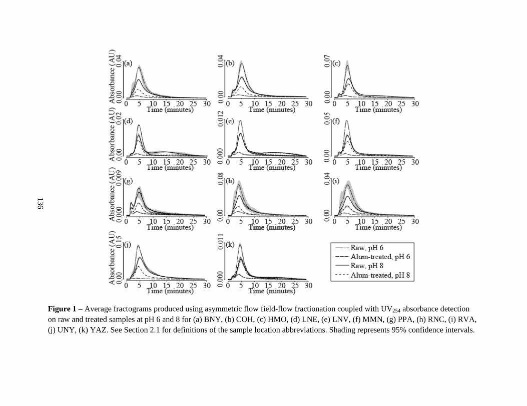
136

Figure 1 – Average fractograms produced using asymmetric flow field-flow fractionation coupled with UV254 absorbance detection on raw and treated samples at pH 6 and 8 for (a) BNY, (b) COH, (c) HMO, (d) LNE, (e) LNV, (f) MMN, (g) PPA, (h) RNC, (i) RVA, (j) UNY, (k) YAZ. See Section 2.1 for definitions of the sample location abbreviations. Shading represents 95% confidence intervals.

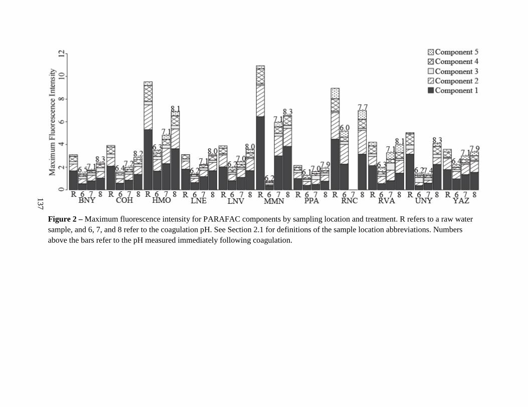
137

Figure 2 – Maximum fluorescence intensity for PARAFAC components by sampling location and treatment. R refers to a raw water sample, and 6, 7, and 8 refer to the coagulation pH. See Section 2.1 for definitions of the sample location abbreviations. Numbers above the bars refer to the pH measured immediately following coagulation.

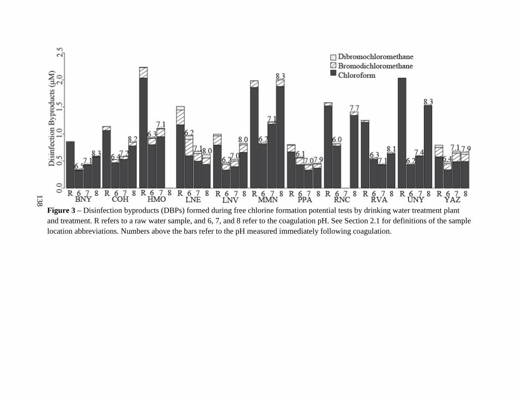
138

Figure 3 – Disinfection byproducts (DBPs) formed during free chlorine formation potential tests by drinking water treatment plant and treatment. R refers to a raw water sample, and 6, 7, and 8 refer to the coagulation pH. See Section 2.1 for definitions of the sample location abbreviations. Numbers above the bars refer to the pH measured immediately following coagulation.

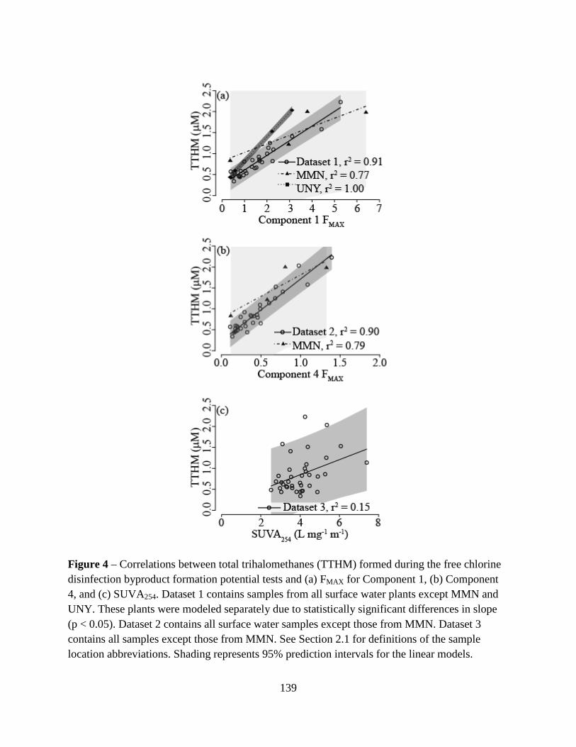
139

Figure 4 – Correlations between total trihalomethanes (TTHM) formed during the free chlorine disinfection byproduct formation potential tests and (a) FMAX for Component 1, (b) Component 4, and (c) SUVA254. Dataset 1 contains samples from all surface water plants except MMN and UNY. These plants were modeled separately due to statistically significant differences in slope (p < 0.05). Dataset 2 contains all surface water samples except those from MMN. Dataset 3 contains all samples except those from MMN. See Section 2.1 for definitions of the sample location abbreviations. Shading represents 95% prediction intervals for the linear models.

140

6. REFERENCES

Aiken, G. and Cotsaris, E., 1995. Soil and hydrology - their effect on NOM. Journal American Water Works Association 87 (1), 36-45.


Apodaca, L. E., Stephens, V. C. and Driver, N. E. (1996). What affects water quality in the Upper Colorado River Basin? United Sates Department of the Interior - United States Geological Survey.

Ates, N., Kitis, M. and Yetis, U., 2007. Formation of chlorination by-products. in waters with low SUVA-correlations with SUVA and differential UV spectroscopy. Water Research 41 (18), 4139-4148.

Beggs, K. M. H. and Summers, R. S., 2011. Character and Chlorine Reactivity of Dissolved Organic Matter from a Mountain Pine Beetle Impacted Watershed. Environmental Science & Technology 45 (13), 5717-5724.

Bond, T., Goslan, E. H., Parsons, S. A. and Jefferson, B., 2010. Disinfection by-product formation of natural organic matter surrogates and treatment by coagulation, MIEX® and nanofiltration. Water Research 44 (5), 1645-1653.

Butler, D. L. and von Guerard, P. (1996). Salinity in the Colorado River in the Grand Valley, Western Colorado, 1994-95. United Sates Department of the Interior - United States Geological Survey.


Chang, E. E., Lin, Y. P. and Chiang, P. C., 2001. Effects of bromide on the formation of THMs and HAAs. Chemosphere 43 (8), 1029-1034.

Chow, A. T., Dahlgren, R. A., Qian, Z. and Wong, P. K., 2008. Relationships between specific ultraviolet absorbance and trihalomethane precursors of different carbon sources. Journal of Water Supply: Research & Technology-AQUA 57 (7), 471-480.

Chow, C. W. K., Fabris, R., Leeuwen, J. v., Wang, D. and Drikas, M., 2008. Assessing Natural Organic Matter Treatability Using High Performance Size Exclusion Chromatography. Environmental Science & Technology 42 (17), 6683-6689.

141

Clow, D. W., Mast, M. A. and Campbell, D. H., 1996. Controls on surface water chemistry in the Upper Merced River Basin, Yosemite National Park, California. Hydrological Processes 10, 727-746.


Eswaran, H., Van Den Berg, E. and Reich, P., 1993. Organic Carbon in Soils of the World. Soil Sci. Soc. Am. J. 57 (1), 192-194.



Korshin, G., Chow, C. W. K., Fabris, R. and Drikas, M., 2009. Absorbance spectroscopy-based examination of effects of coagulation on the reactivity of fractions of natural organic matter with varying apparent molecular weights. Water Research 43 (6), 1541-1548.

Miller, M. P. and McKnight, D. M., 2010. Comparison of seasonal changes in fluorescent dissolved organic matter among aquatic lake and stream sites in the Green Lakes Valley. J. Geophys. Res. 115, G00F12.

Mohawk Valley Water Authority (2011). Water Quality Report 2011. Utica.

Murphy, K. R., Ruiz, G. M., Dunsmuir, W. T. M. and Waite, T. D., 2006. Optimized Parameters for Fluorescence-Based Verification of Ballast Water Exchange by Ships. Environmental Science & Technology 40 (7), 2357-2362.

Natural Resource Conservation Service. "Distribution Maps of Dominant Soil Orders." Retrieved June 5, 2012, from http://soils.usda.gov/technical/classification/orders/.


142




Stedmon, C. A., Markager, S. and Bro, R., 2003. Tracing dissolved organic matter in aquatic environments using a new approach to fluorescence spectroscopy. Marine Chemistry 82 (3-4), 239-254.


Weishaar, J. L., Aiken, G. R., Bergamaschi, B. A., Fram, M. S., Fujii, R. and Mopper, K., 2003. Evaluation of Specific Ultraviolet Absorbance as an Indicator of the Chemical Composition and Reactivity of Dissolved Organic Carbon. Environmental Science & Technology 37 (20), 4702-4708.

Yang, Z., Gao, B. and Yue, Q., 2010. Coagulation performance and residual aluminum speciation of Al2(SO4)3 and polyaluminum chloride (PAC) in Yellow River water treatment. Chemical Engineering Journal 165 (1), 122-132.


143

APPENDIX 3

Supporting Information for

“Assessing Fluorescence-PARAFAC for Prediction of Disinfection Byproduct Formation

Potential in Drinking Water from Diverse Watersheds”

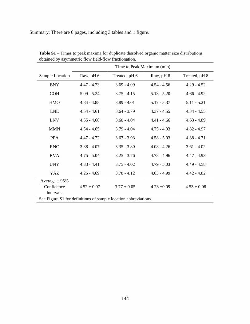
144

Summary: There are 6 pages, including 3 tables and 1 figure.

Table S1 – Times to peak maxima for duplicate dissolved organic matter size distributions obtained by asymmetric flow field-flow fractionation.

Time to Peak Maximum (min)

Sample Location Raw, pH 6 Treated, pH 6 Raw, pH 8 Treated, pH 8

BNY 4.47 - 4.73 3.69 - 4.09 4.54 - 4.56 4.29 - 4.52

COH 5.09 - 5.24 3.75 - 4.15 5.13 - 5.20 4.66 - 4.92

HMO 4.84 - 4.85 3.89 - 4.01 5.17 - 5.37 5.11 - 5.21

LNE 4.54 - 4.61 3.64 - 3.79 4.37 - 4.55 4.34 - 4.55

LNV 4.55 - 4.68 3.60 - 4.04 4.41 - 4.66 4.63 - 4.89

MMN 4.54 - 4.65 3.79 - 4.04 4.75 - 4.93 4.82 - 4.97

PPA 4.47 - 4.72 3.67 - 3.93 4.58 - 5.03 4.38 - 4.71

RNC 3.88 - 4.07 3.35 - 3.80 4.08 - 4.26 3.61 - 4.02

RVA 4.75 - 5.04 3.25 - 3.76 4.78 - 4.96 4.47 - 4.93

UNY 4.33 - 4.41 3.75 - 4.02 4.79 - 5.03 4.49 - 4.58

YAZ 4.25 - 4.69 3.78 - 4.12 4.63 - 4.99 4.42 - 4.82

Average ± 95% Confidence Intervals

4.52 ± 0.07 3.77 ± 0.05 4.73 ±0.09 4.53 ± 0.08

See Figure S1 for definitions of sample location abbreviations.

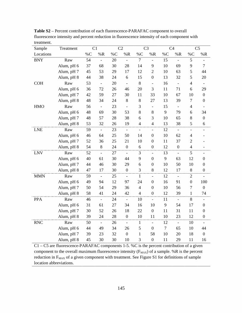
145

Table S2 – Percent contribution of each fluorescence-PARAFAC component to overall fluorescence intensity and percent reduction in fluorescence intensity of each component with treatment. Sample Locations

Treatment C1 C2 C3 C4 C5 %C %R %C %R %C %R %C %R %C %R

BNY Raw 54 - 20 - 7 - 15 - 5 - Alum, pH 6 37 68 30 28 14 9 10 69 9 7 Alum, pH 7 45 53 29 17 12 2 10 63 5 44 Alum, pH 8 44 38 24 6 15 0 13 32 5 20

COH Raw 53 - 20 - 8 - 16 - 4 - Alum, pH 6 36 72 26 46 20 3 11 71 6 29 Alum, pH 7 42 59 27 30 11 33 10 67 10 0 Alum, pH 8 48 34 24 8 8 27 13 39 7 0

HMO Raw 56 - 23 - 3 - 15 - 4 - Alum, pH 6 48 69 30 53 8 8 9 79 6 34 Alum, pH 7 48 57 28 38 6 3 10 65 8 0 Alum, pH 8 53 32 26 19 4 4 13 38 5 6

LNE Raw 59 - 23 - - - 12 - - - Alum, pH 6 46 64 25 50 14 0 10 62 4 - Alum, pH 7 52 36 25 21 10 0 11 37 2 - Alum, pH 8 54 8 24 0 6 0 12 0 4 -

LNV Raw 52 - 27 - 3 - 13 - 5 - Alum, pH 6 40 61 30 44 9 0 9 63 12 0 Alum, pH 7 44 46 30 29 6 0 10 50 10 0 Alum, pH 8 47 17 30 0 3 8 12 17 8 0

MMN Raw 59 - 25 - 1 - 12 - 2 - Alum, pH 6 49 94 12 97 24 0 16 91 0 100 Alum, pH 7 50 54 29 36 4 0 10 56 7 0 Alum, pH 8 58 41 24 42 4 0 12 39 1 74

PPA Raw 46 - 24 - 10 - 11 - 8 - Alum, pH 6 31 61 27 34 16 10 9 54 17 0 Alum, pH 7 30 52 26 18 22 0 11 31 11 0 Alum, pH 8 39 24 28 0 10 11 10 23 12 0

RNC Raw 50 - 26 - 1 - 12 - 10 - Alum, pH 6 44 49 34 26 5 0 7 65 10 44 Alum, pH 7 39 23 32 0 1 58 10 20 18 0 Alum, pH 8 45 30 30 10 3 0 11 29 11 16

C1 – C5 are fluorescence-PARAFAC components 1-5. %C is the percent contribution of a given component to the overall maximum fluorescence intensity (FMAX ) of a sample. %R is the percent reduction in FMAX of a given component with treatment. See Figure S1 for definitions of sample location abbreviations.

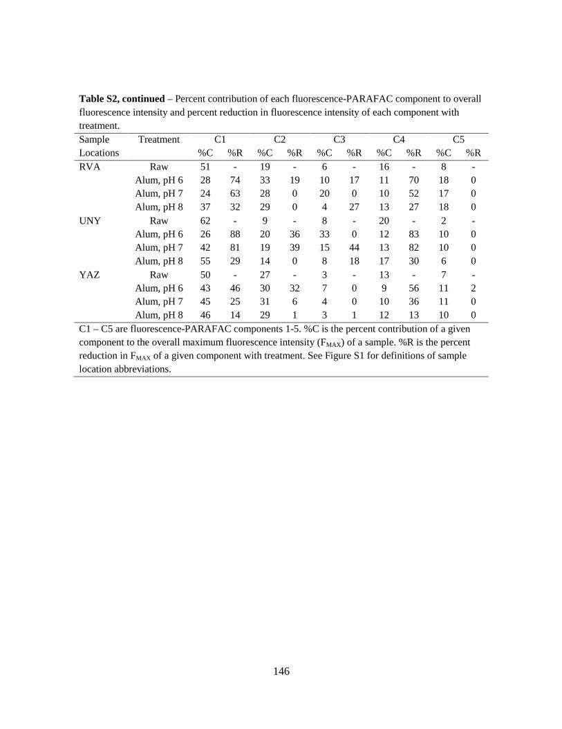
146

Table S2, continued – Percent contribution of each fluorescence-PARAFAC component to overall fluorescence intensity and percent reduction in fluorescence intensity of each component with treatment. Sample Treatment C1 C2 C3 C4 C5 Locations %C %R %C %R %C %R %C %R %C %R RVA Raw 51 - 19 - 6 - 16 - 8 -

Alum, pH 6 28 74 33 19 10 17 11 70 18 0 Alum, pH 7 24 63 28 0 20 0 10 52 17 0 Alum, pH 8 37 32 29 0 4 27 13 27 18 0

UNY Raw 62 - 9 - 8 - 20 - 2 - Alum, pH 6 26 88 20 36 33 0 12 83 10 0 Alum, pH 7 42 81 19 39 15 44 13 82 10 0 Alum, pH 8 55 29 14 0 8 18 17 30 6 0

YAZ Raw 50 - 27 - 3 - 13 - 7 - Alum, pH 6 43 46 30 32 7 0 9 56 11 2 Alum, pH 7 45 25 31 6 4 0 10 36 11 0 Alum, pH 8 46 14 29 1 3 1 12 13 10 0 C1 – C5 are fluorescence-PARAFAC components 1-5. %C is the percent contribution of a given component to the overall maximum fluorescence intensity (FMAX ) of a sample. %R is the percent reduction in FMAX of a given component with treatment. See Figure S1 for definitions of sample location abbreviations.

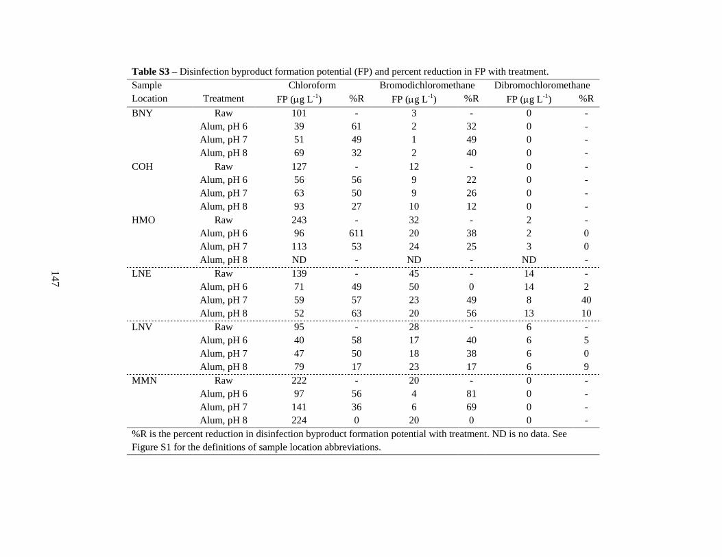
147

Table S3 – Disinfection byproduct formation potential (FP) and percent reduction in FP with treatment. Sample Chloroform Bromodichloromethane Dibromochloromethane Location Treatment FP (µg L-1) %R FP (µg L-1) %R FP (µg L-1) %R

BNY Raw 101 - 3 - 0 - Alum, pH 6 39 61 2 32 0 - Alum, pH 7 51 49 1 49 0 - Alum, pH 8 69 32 2 40 0 - COH Raw 127 - 12 - 0 - Alum, pH 6 56 56 9 22 0 - Alum, pH 7 63 50 9 26 0 - Alum, pH 8 93 27 10 12 0 - HMO Raw 243 - 32 - 2 - Alum, pH 6 96 611 20 38 2 0 Alum, pH 7 113 53 24 25 3 0 Alum, pH 8 ND - ND - ND - LNE Raw 139 - 45 - 14 - Alum, pH 6 71 49 50 0 14 2 Alum, pH 7 59 57 23 49 8 40 Alum, pH 8 52 63 20 56 13 10 LNV Raw 95 - 28 - 6 - Alum, pH 6 40 58 17 40 6 5 Alum, pH 7 47 50 18 38 6 0 Alum, pH 8 79 17 23 17 6 9 MMN Raw 222 - 20 - 0 - Alum, pH 6 97 56 4 81 0 - Alum, pH 7 141 36 6 69 0 - Alum, pH 8 224 0 20 0 0 - %R is the percent reduction in disinfection byproduct formation potential with treatment. ND is no data. See Figure S1 for the definitions of sample location abbreviations.

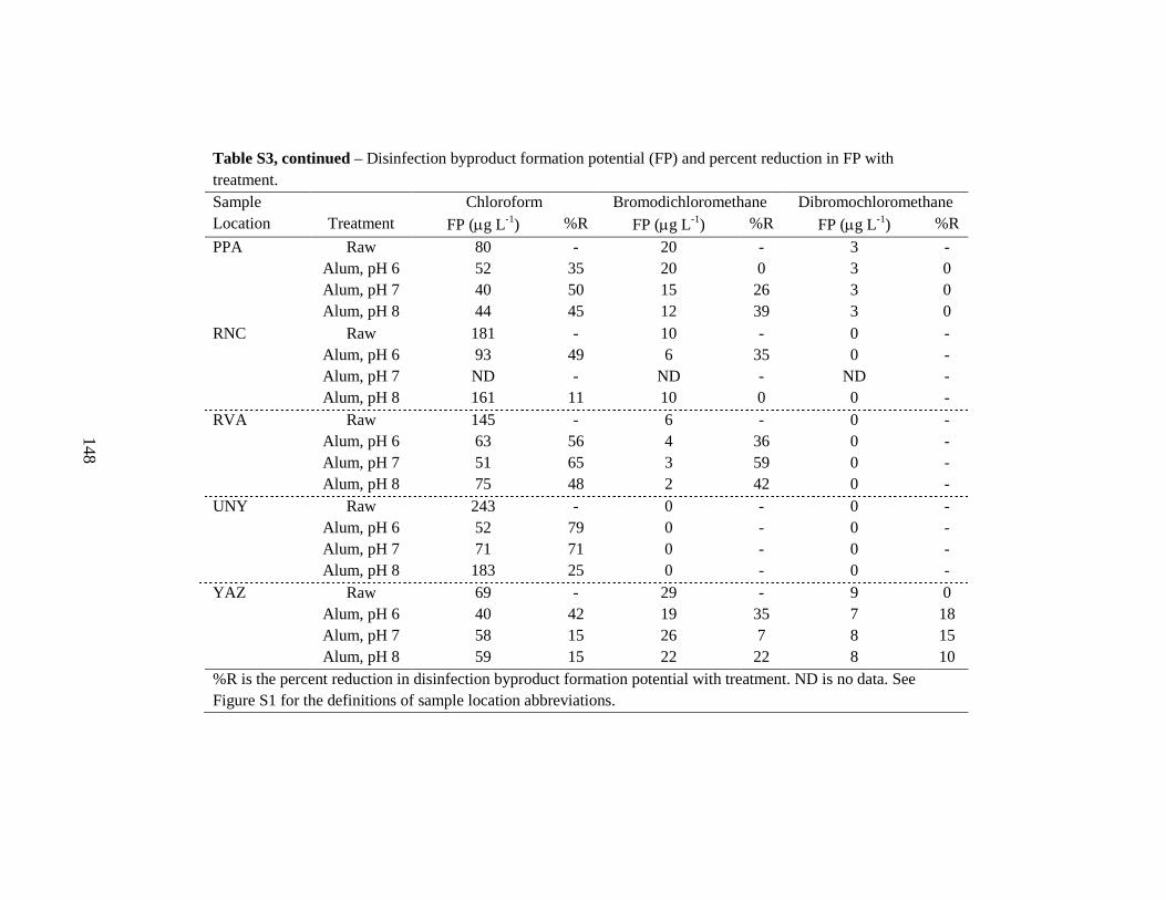
148

Table S3, continued – Disinfection byproduct formation potential (FP) and percent reduction in FP with treatment. Sample Chloroform Bromodichloromethane Dibromochloromethane Location Treatment FP (µg L-1) %R FP (µg L-1) %R FP (µg L-1) %R

PPA Raw 80 - 20 - 3 - Alum, pH 6 52 35 20 0 3 0 Alum, pH 7 40 50 15 26 3 0 Alum, pH 8 44 45 12 39 3 0 RNC Raw 181 - 10 - 0 - Alum, pH 6 93 49 6 35 0 - Alum, pH 7 ND - ND - ND - Alum, pH 8 161 11 10 0 0 - RVA Raw 145 - 6 - 0 - Alum, pH 6 63 56 4 36 0 - Alum, pH 7 51 65 3 59 0 - Alum, pH 8 75 48 2 42 0 - UNY Raw 243 - 0 - 0 - Alum, pH 6 52 79 0 - 0 - Alum, pH 7 71 71 0 - 0 -

Alum, pH 8 183 25 0 - 0 - YAZ Raw 69 - 29 - 9 0 Alum, pH 6 40 42 19 35 7 18 Alum, pH 7 58 15 26 7 8 15 Alum, pH 8 59 15 22 22 8 10 %R is the percent reduction in disinfection byproduct formation potential with treatment. ND is no data. See Figure S1 for the definitions of sample location abbreviations.

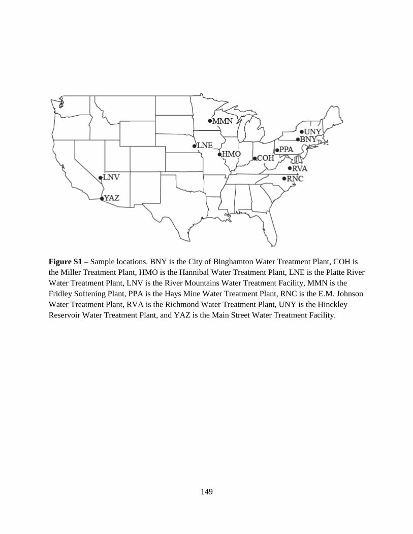
149

Figure S1 – Sample locations. BNY is the City of Binghamton Water Treatment Plant, COH is the Miller Treatment Plant, HMO is the Hannibal Water Treatment Plant, LNE is the Platte River Water Treatment Plant, LNV is the River Mountains Water Treatment Facility, MMN is the Fridley Softening Plant, PPA is the Hays Mine Water Treatment Plant, RNC is the E.M. Johnson Water Treatment Plant, RVA is the Richmond Water Treatment Plant, UNY is the Hinckley Reservoir Water Treatment Plant, and YAZ is the Main Street Water Treatment Facility.

150

CHAPTER 6

Conclusion

151

1. SUMMARY

In this work, dissolved organic matter (DOM) was physically and chemically

characterized before and after enhanced coagulation and magnetic ion exchange resin (MIEX®)

treatments. Two relatively new characterization techniques, asymmetric flow-field flow

fractionation (AF4) and fluorescence-parallel factor (PARAFAC) analysis, were used throughout

this work. Both techniques required low sample volumes and no pre-concentration or extreme

pH perturbations, which made the analysis of laboratory-treated samples representative of actual

drinking water treatment conditions. These techniques provided insights into the impacts of

treatment on DOM size distributions and chemical composition.

Disinfection byproduct (DBP) formation potential (FP) tests on raw and treated samples

were conducted using free chlorine, and DBPFP was correlated to the maximum fluorescence

intensity (FMAX ) of PARAFAC components. In Chapter 3, strong correlations were discovered

between chloroform FP and fluorescence components from a set of raw and alum-coagulated

waters from Beaver Lake. This work was expanded in Chapter 4 to include chloroform FP and

fluorescence-PARAFAC data from a MIEX® study which used the same raw waters from Beaver

Lake, and the correlations were affirmed. Lastly, in Chapter 5, raw water samples were collected

from drinking water sources across the United States and were treated by alum coagulation

followed by chlorination in Chapter 5, and strong linear correlations between DBPFP and

fluorescence-PARAFAC components were discovered. The work reported in Chapters 4 and 5

were novel validations of the PARAFAC model and were valuable steps towards an improved

DBPFP surrogate for use in drinking water treatment plants (DWTPs).

152

1.1. Objective 1 – Development of AF4 and fluorescence-PARAFAC methods

In Chapter 2, detailed methods were developed to characterize chromophoric DOM

(CDOM) physically using AF4 (with a 300 Da membrane) coupled with ultraviolet absorbance

at 254 nm (UV254) and chemically using fluorescence-PARAFAC. These methods were validated

by application to Beaver Lake water samples collected from three depths (3, 10, and 18 m below

the surface) over a period of 8 weeks. The CDOM at 10 m had the highest AF4-UV254 peak

maxima and highest fluorescence intensities, which indicated that CDOM was stratified by depth

in Beaver Lake.

In Chapter 3, AF4 methods were adjusted to accommodate a 1,000 Da membrane, which

improved the stability of the instrument and reproducibility of AF4-UV254 fractograms. In

addition, the impact of eluent composition became apparent. Raw water samples were

fractionated in phosphate-carbonate buffer solutions at pH 6 and 8 with conductivities of 470 µS

cm-1. Peaks from samples fractionated at pH 6 were consistently higher than at pH 8, which

indicated that pH control was important for comparisons of fractograms (e.g. raw vs. treated

samples). In Chapter 5, AF4-UV254 showed differences in relative sizes of CDOM from eleven

drinking water sources, further validating the methods.

1.2. Objective 2 – Impact of treatment on DOM properties

In Chapter 3, raw waters from four drinking water treatment plants on Beaver Lake were

subjected to alum coagulation at pH 6, 7, and 8. AF4-UV254 fractograms showed that alum

coagulation at pH 6 consistently removed more CDOM than at pH 8. In addition, alum

coagulation at pH 6 preferentially removed larger CDOM, while CDOM removal was more

uniform at pH 8. Fluorescence-PARAFAC identified one protein-like and three humic-like

153

components in Beaver Lake DOM. All four components were more effectively removed at pH 6

than at pH 8, and a humic-like component, C1, was preferentially removed by alum coagulation.

In Chapter 4, MIEX®-treated Beaver Lake water samples were compared to the alum

treated samples from Chapter 3 to test the applicability of PARAFAC across fundamentally

different treatment regimes. Two PARAFAC models were constructed: (1) Model 1, from raw

and MIEX-treated samples, and (2) Model 3, from raw, MIEX®-treated, and alum-treated

samples. These models were compared to Model 2, from raw and alum-treated samples. Similar

components were identified for Models 1 and 2, and the larger dataset contributing to Model 3

resulted in resolution of an additional component. MIEX® treatment at pH 6, 7, and 8 removed

DOM with no pH impacts observable using fluorescence-PARAFAC. DOM removal using

MIEX® at pH 6, 7, and 8 was similar to that of alum coagulation at pH 6. However, a set of

samples from a heavy rainfall event contained relatively high levels of a PARAFAC component,

and this component was more effectively removed by alum than by MIEX®.

In Chapter 5, raw water samples from eleven DWTPs from across the United States were

subjected to alum coagulation at pH 6, 7, and 8. AF4-UV254 fractionation of raw and treated

waters at pH 6 and 8 indicated that more CDOM was removed at pH 6 than at pH 8. Further,

alum coagulation at pH 6 preferentially removed larger CDOM for all source waters. Although

alum coagulation at pH 8 resulted in preferential removal of large CDOM for some source

waters, the CDOM size distributions shifted toward larger CDOM for two source waters.

Fluorescence-PARAFAC identified three humic-like components and two protein-like

components, and indicated consistent, preferential removal of two of the humic-like components

by alum coagulation.

154

1.3. Objective 3 – DBPFP-PARAFAC correlations for alum-treated waters

In Chapter 3, strong correlations (r2 = 0.84) were developed between a humic-like

PARAFAC component (C1) and chloroform FP. These correlations were an improvement on

chloroform FP-SUVA254 correlations (r2 = 0.51) and chloroform FP-chlorine demand

correlations (r2 = 0.58).

1.4. Objective 4 – Validation of DBPFP-PARAFAC correlations for two DOM removal

processes

In Chapter 4, correlations between C1 and chloroform FP for Models 1, 2, and 3 were

statistically similar and strong (e.g., r2 = 0.87 for Model 3). However, chloroform FP and

SUVA254 for Model 1 were uncorrelated (r2 = 0.00). These results indicated that C1 was an

effective chloroform FP surrogate for alum and MIEX® treatments and was a significant

improvement over SUVA254.

1.5. Objective 5 – Validation of DBPFP-PARAFAC correlations for eleven source waters

In Chapter 5, correlations were developed between total trihalomethane (TTHM) FP and

PARAFAC components. Analysis of covariance (ANCOVA) indicated that one linear model (r2

= 0.91) could describe TTHMFP-C1 correlations for eight of eleven source waters. This linear

model was statistically similar to the models produced in Chapters 3 and 4. C1 from the lone

groundwater source (LNE) was uncorrelated to TTHMFP. Two other water sources (MMN and

UNY) produced separate linear models relating C1 and TTHMFP. For SUVA254 and TTHMFP, a

single linear model (r2 = 0.15) was used for 10 of the 11 source waters. C1 for MMN was

uncorrelated to TTHMFP. Interestingly, The LNE and MMN samples both came from

watersheds dominated by Mollisols, and the UNY sample was the sole sample from a watershed

155

dominated by Spodosols. These results indicated that fluorescence-PARAFAC was a more

broadly applicable TTHMFP surrogate than SUVA254.

SIGNIFICANCE AND FUTURE WORK

The conclusions from this work are valuable additions to the current understanding of

DOM characterization, the impacts of treatment on DOM properties and the relationship between

DOM properties and DBPFP. The pH effects observed during DOM size characterizations using

AF4 indicate the importance of pH to CDOM behavior and must be kept in mind when

comparing CDOM size distributions. This highlighted the usefulness of AF4 for understanding

CDOM in natural and engineered systems because fractionation can be done over a range of pH

values applicable to drinking water treatment. Future studies to better understand the impacts of

pH on CDOM properties would be beneficial to characterizations of DOM in natural waters as

well as optimization of DOM removal processes.

DBPFP-PARAFAC component correlations were shown to be an improvement over

DBPFP-SUVA254 correlations for two DOM removal processes and a variety of water sources.

Future studies could include investigation of source waters from Mollisol- and Spodosol-

dominated watersheds to determine if more broadly applicable DBPFP-PARAFAC component

correlations could be developed specifically for watersheds containing those soils.

Currently, fluorescence-PARAFAC is of limited use to DWTPs, but it would likely be

useful for optimization of processes in addition to DBP precursor removal. Although it could be

used for long-term process optimization studies, pilot studies of online fluorescence detectors

and development of PARAFAC models capable of resolving specified components in single

samples are needed before this technique could be used in daily DWTP operations.

Documents

New Insights into Disinfection Byproduct Formation and