NIF Target Diagnostic Automated Analysis:

Transitioning to a User Facility

Presentation to

CASIS

May 21, 2014

LLNL-PRES-654645

Judith Liebman, Rita Bettenhausen, Essex Bond, Allan Casey, Robert

Fallejo, Matt Hutton, Amber Marsh, Abbie Warrick

Automated diagnostic analysis is used to estimate NIF

experimental key performance metrics and enable facility

optimization

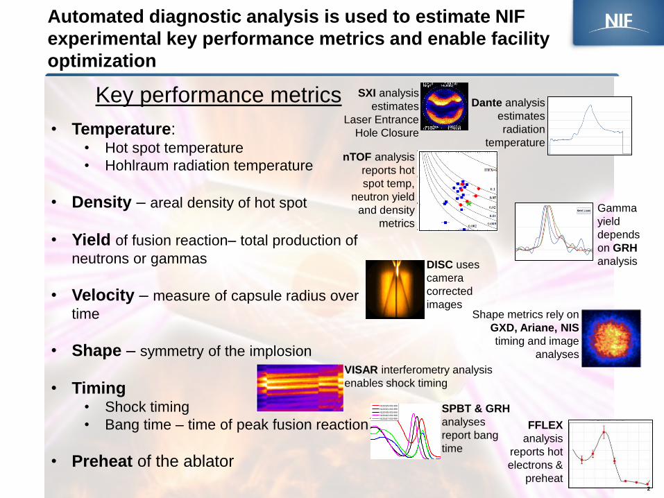
Key performance metrics

• Temperature: • Hot spot temperature

• Hohlraum radiation temperature

• Density – areal density of hot spot

• Yield of fusion reaction– total production of

neutrons or gammas

• Velocity – measure of capsule radius over

time

• Shape – symmetry of the implosion

• Timing • Shock timing

• Bang time – time of peak fusion reaction

• Preheat of the ablator

VISAR interferometry analysis

enables shock timing

FFLEX

analysis

reports hot

electrons &

preheat

21.5 22 22.5 23 23.50

5

10

15

20

25

30

Time (ns)

Deconv. S

ignal (V

)

SPBT

N120329-001-999

N120321-001-999

N120405-003-999

N120412-001-999

N120417-002-999

SPBT & GRH

analyses

report bang

time

DISC uses

camera

corrected

images Shape metrics rely on

GXD, Ariane, NIS

timing and image

analyses

Dante analysis

estimates

radiation

temperature

Gamma

yield

depends

on GRH

analysis

nTOF analysis

reports hot

spot temp,

neutron yield

and density

metrics

2

SXI analysis

estimates

Laser Entrance

Hole Closure

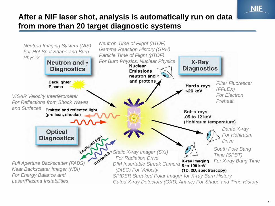
After a NIF laser shot, analysis is automatically run on data

from more than 20 target diagnostic systems

Full Aperture Backscatter (FABS)

Near Backscatter Imager (NBI)

For Energy Balance and

Laser/Plasma Instabilities

Filter Fluorescer

(FFLEX)

For Electron

Preheat

Dante X-ray

For Hohlraum

Drive

VISAR Velocity Interferometer

For Reflections from Shock Waves

and Surfaces

Neutron Time of Flight (nTOF)

Gamma Reaction History (GRH)

Particle Time of Flight (pTOF)

For Burn Physics, Nuclear Physics

Static X-ray Imager (SXI)

For Radiation Drive

DIM Insertable Streak Camera

(DISC) For Velocity

SPIDER Streaked Polar Imager for X-ray Burn History

Gated X-ray Detectors (GXD, Ariane) For Shape and Time History

South Pole Bang

Time (SPBT)

For X-ray Bang Time

and protons

Neutron Imaging System (NIS)

For Hot Spot Shape and Burn

Physics

3

Overview from study on shifts needed for diagnostic

scientists, setup, and analysis to support the NIF user facility

• Full automation of diagnostics is feasible with minimum loss of data quality

— Deliver defined standard analysis results within stated errors

— Stretch analysis goals may be compromised (e.g. NTOF velocity)

• Templates can be used to set up diagnostics with little risk to equipment

— Restrict use of some templates based on set up values such as laser energy

or neutron yield

• All diagnostics require some scientist support to achieve automation

— Implement templates and automated approval

— Analysis requirements updates

— Update calibrations used for automated analysis

— Guidelines and estimators for diagnostic set up

• Implementation will require a cultural change

— Program not blame diagnostic scientist for operations failure

— Diagnostic scientist accept operations failure due to incorrect set up

— Diagnostic scientists fully adopt automated processing instead of

rerunning manual analysis

Author—NIC Review, December 2014 4 NIF-0000-00000s2.ppt

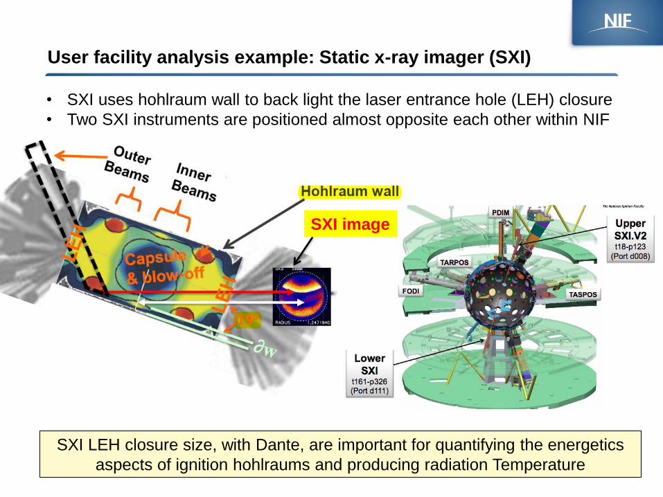
User facility analysis example: Static x-ray imager (SXI)

• SXI uses hohlraum wall to back light the laser entrance hole (LEH) closure

• Two SXI instruments are positioned almost opposite each other within NIF

SXI LEH closure size, with Dante, are important for quantifying the energetics

aspects of ignition hohlraums and producing radiation Temperature

SXI image

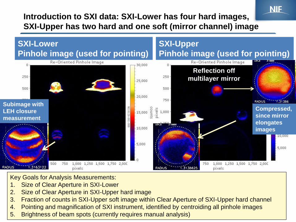
Introduction to SXI data: SXI-Lower has four hard images,

SXI-Upper has two hard and one soft (mirror channel) image

SXI-Upper

Pinhole image (used for pointing)

SXI-Lower

Pinhole image (used for pointing)

Reflection off

multilayer mirror

Subimage with

LEH closure

measurement

Compressed,

since mirror

elongates

images

Key Goals for Analysis Measurements:

1. Size of Clear Aperture in SXI-Lower

2. Size of Clear Aperture in SXI-Upper hard image

3. Fraction of counts in SXI-Upper soft image within Clear Aperture of SXI-Upper hard channel

4. Pointing and magnification of SXI instrument, identified by centroiding all pinhole images

5. Brightness of beam spots (currently requires manual analysis)

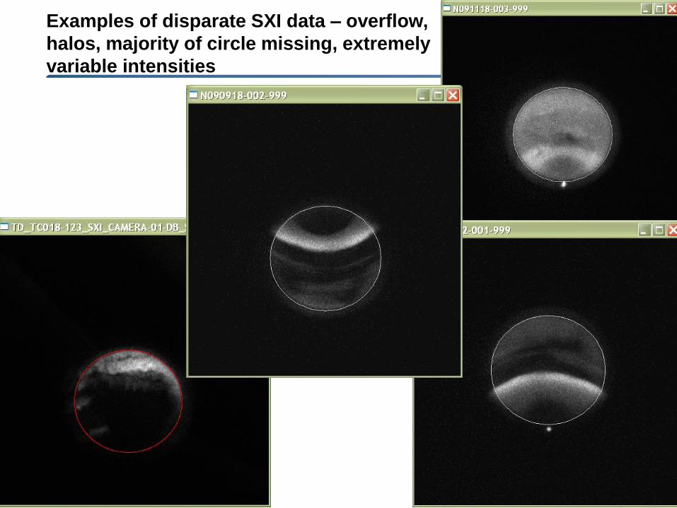
Examples of disparate SXI data – overflow,

halos, majority of circle missing, extremely

variable intensities

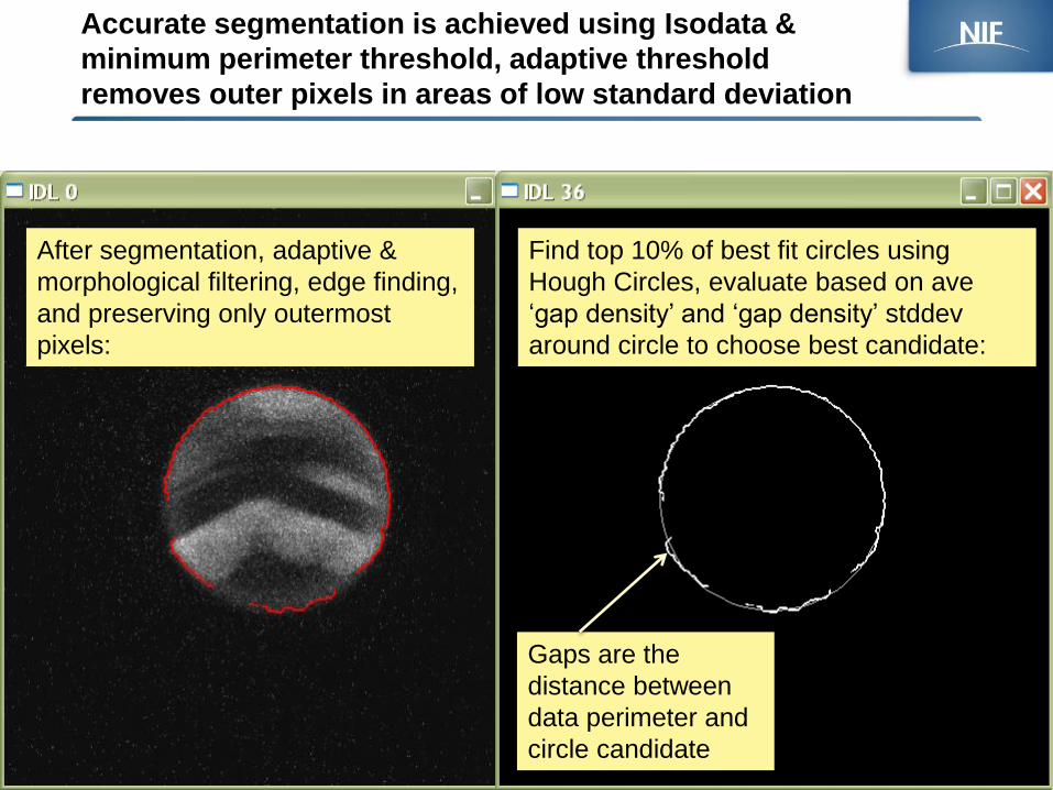
Accurate segmentation is achieved using Isodata &

minimum perimeter threshold, adaptive threshold

removes outer pixels in areas of low standard deviation

After segmentation, adaptive &

morphological filtering, edge finding,

and preserving only outermost

pixels:

Find top 10% of best fit circles using

Hough Circles, evaluate based on ave

‘gap density’ and ‘gap density’ stddev

around circle to choose best candidate:

Gaps are the

distance between

data perimeter and

circle candidate

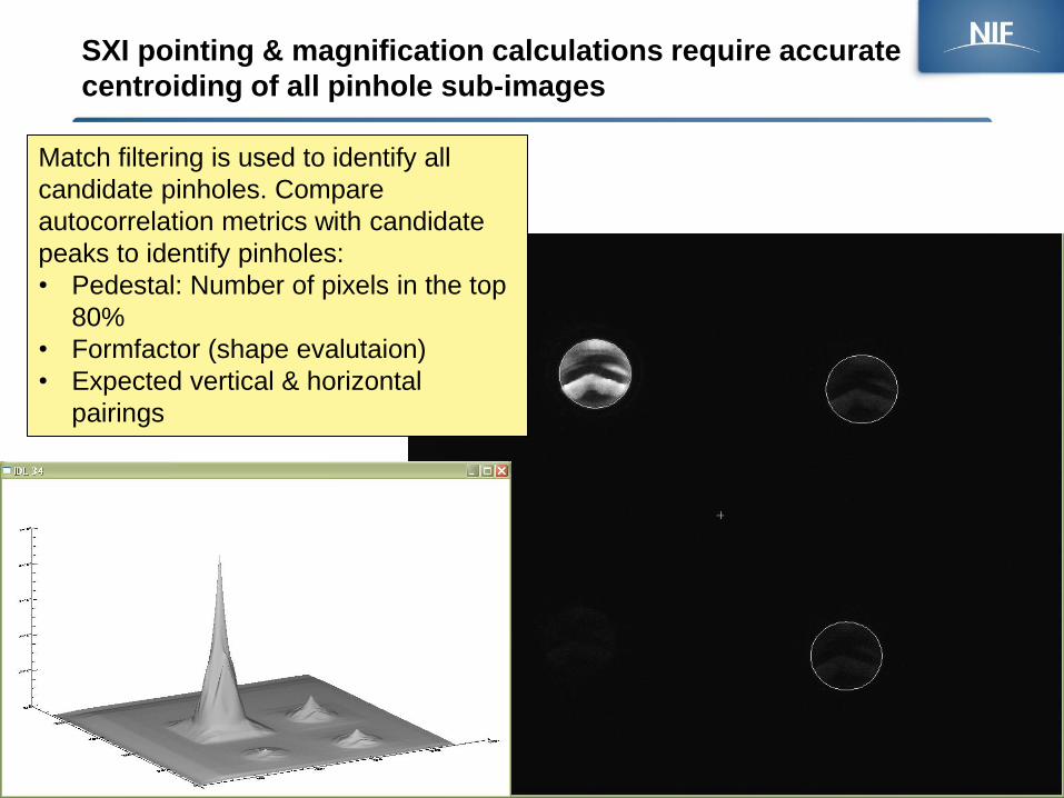
SXI pointing & magnification calculations require accurate

centroiding of all pinhole sub-images

Match filtering is used to identify all

candidate pinholes. Compare

autocorrelation metrics with candidate

peaks to identify pinholes:

• Pedestal: Number of pixels in the top

80%

• Formfactor (shape evalutaion)

• Expected vertical & horizontal

pairings

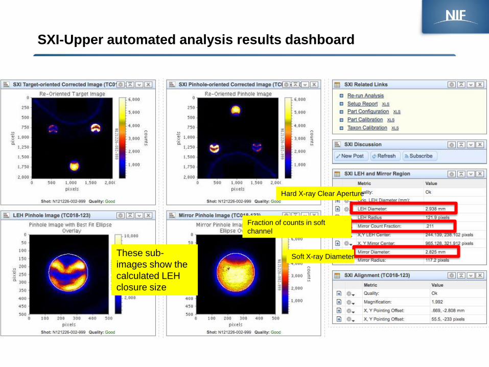
SXI-Upper automated analysis results dashboard

These sub-

images show the

calculated LEH

closure size

Hard X-ray Clear Aperture

Fraction of counts in soft

channel

Soft X-ray Diameter

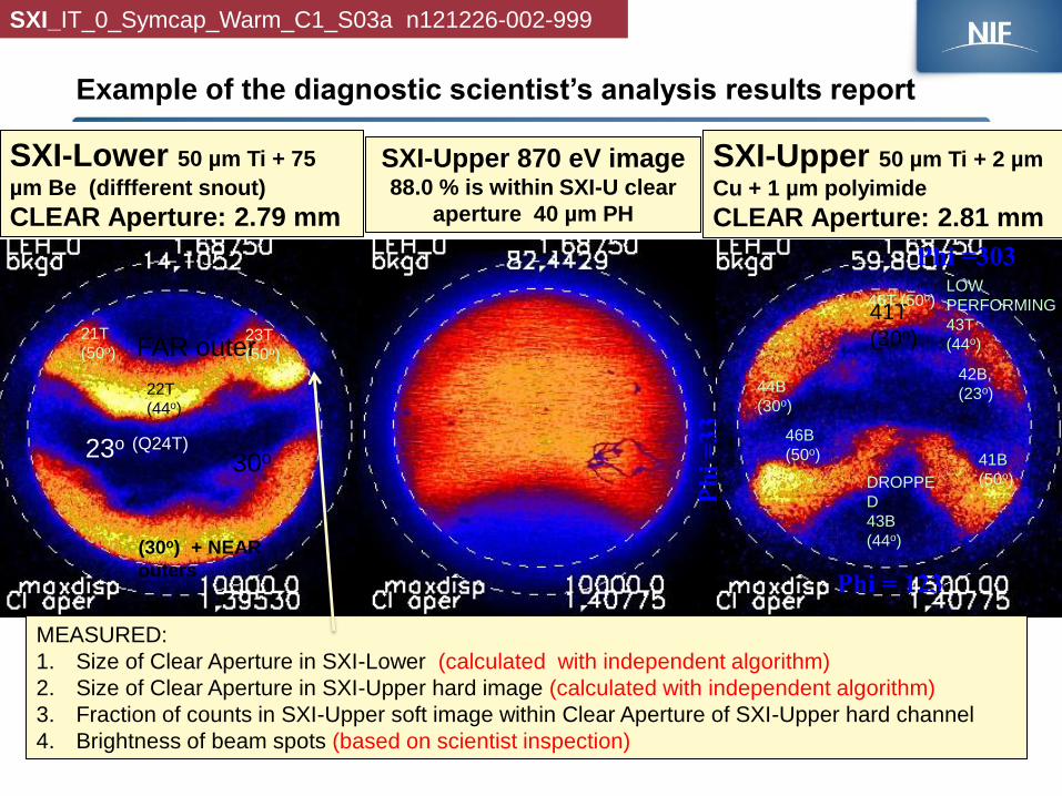
SXI-Upper 50 µm Ti + 2 µm

Cu + 1 µm polyimide

CLEAR Aperture: 2.81 mm

MEASURED:

1. Size of Clear Aperture in SXI-Lower (calculated with independent algorithm)

2. Size of Clear Aperture in SXI-Upper hard image (calculated with independent algorithm)

3. Fraction of counts in SXI-Upper soft image within Clear Aperture of SXI-Upper hard channel

4. Brightness of beam spots (based on scientist inspection)

SXI-Upper 870 eV image 88.0 % is within SXI-U clear

aperture 40 µm PH

Ph

i =

33

Phi =303

41T

(30o)

44B

(30o)

42B,

(23o)

DROPPE

D

43B

(44o)

41B

(50o)

46B

(50o)

46T (50o) LOW

PERFORMING

43T

(44o)

Phi = 123

SXI-Lower 50 µm Ti + 75

µm Be (diffferent snout)

CLEAR Aperture: 2.79 mm

(30o) + NEAR

outers

30o 23o (Q24T)

FAR outer

22T

(44o)

23T

(50o)

21T

(50o)

SXI_IT_0_Symcap_Warm_C1_S03a n121226-002-999

Example of the diagnostic scientist’s analysis results report

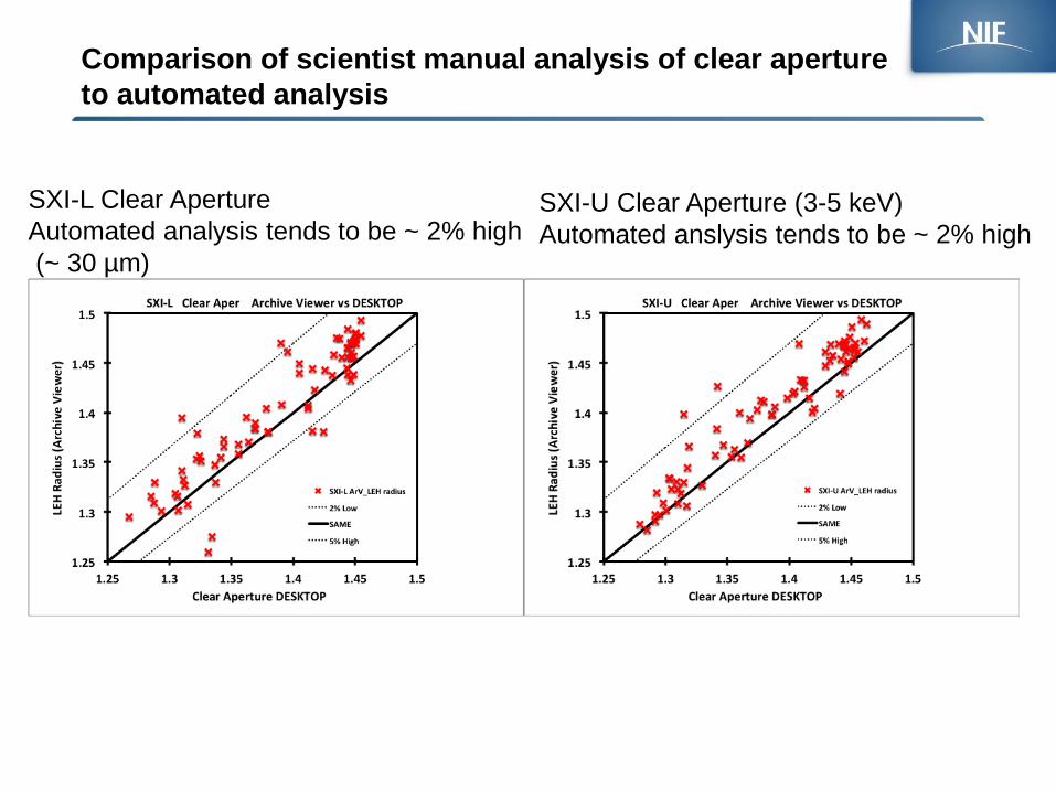
Comparison of scientist manual analysis of clear aperture

to automated analysis

SXI-L Clear Aperture

Automated analysis tends to be ~ 2% high

(~ 30 µm)

SXI-U Clear Aperture (3-5 keV)

Automated anslysis tends to be ~ 2% high

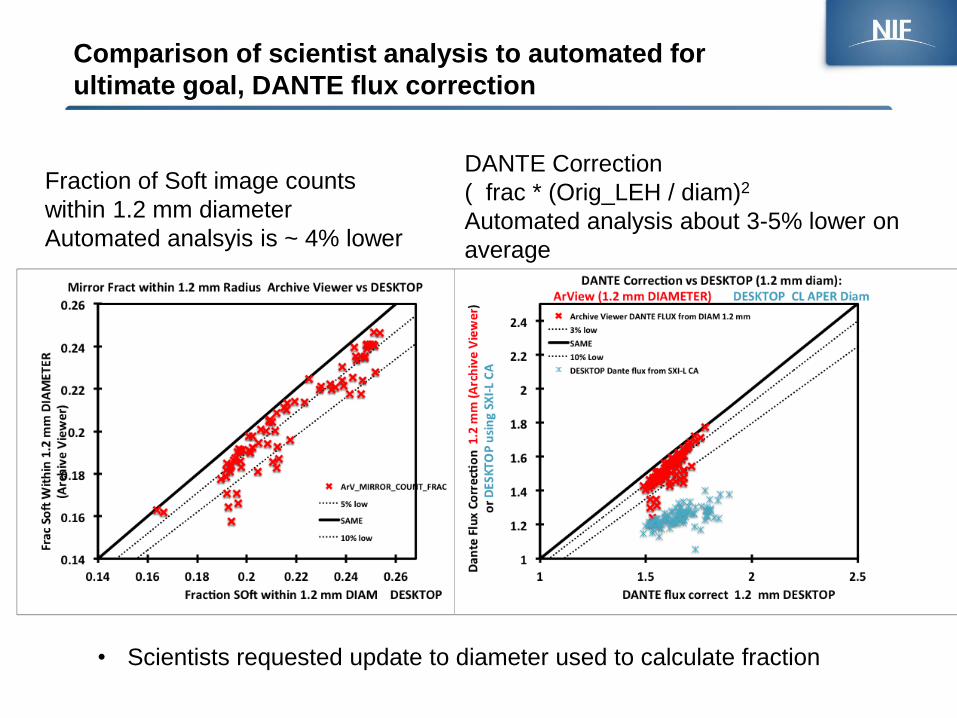
Comparison of scientist analysis to automated for

ultimate goal, DANTE flux correction

Fraction of Soft image counts

within 1.2 mm diameter

Automated analsyis is ~ 4% lower

DANTE Correction

( frac * (Orig_LEH / diam)2

Automated analysis about 3-5% lower on

average

• Scientists requested update to diameter used to calculate fraction

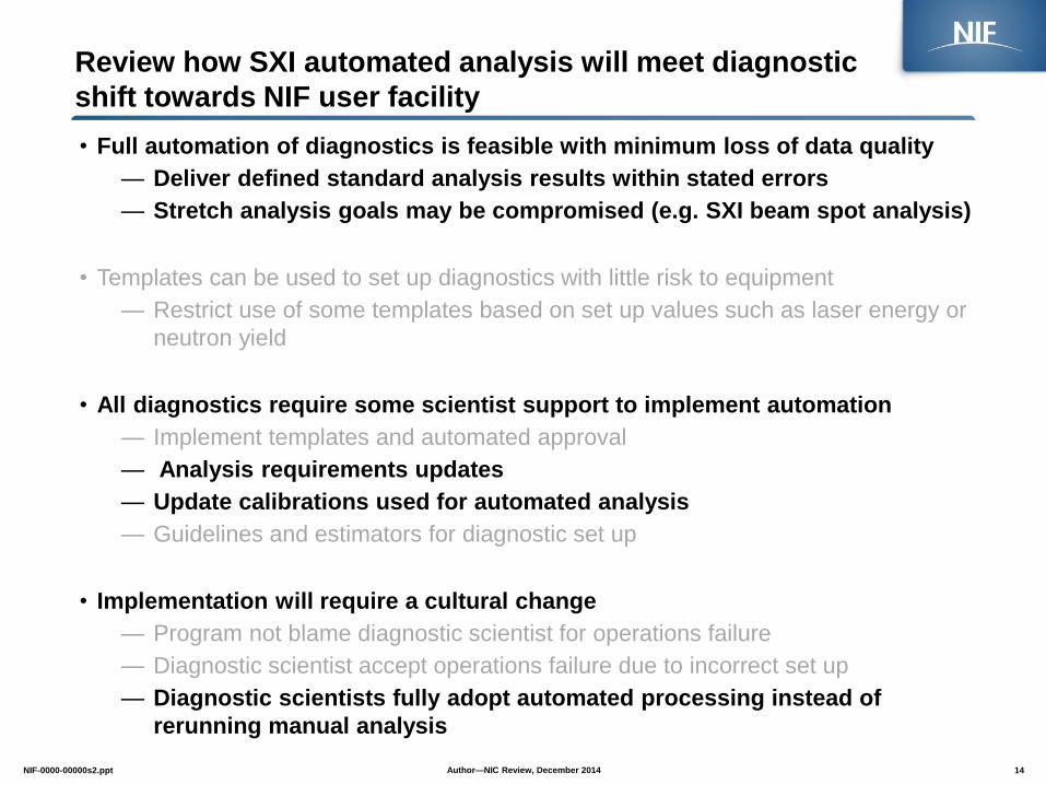
Review how SXI automated analysis will meet diagnostic

shift towards NIF user facility

• Full automation of diagnostics is feasible with minimum loss of data quality

— Deliver defined standard analysis results within stated errors

— Stretch analysis goals may be compromised (e.g. SXI beam spot analysis)

• Templates can be used to set up diagnostics with little risk to equipment

— Restrict use of some templates based on set up values such as laser energy or

neutron yield

• All diagnostics require some scientist support to implement automation

— Implement templates and automated approval

— Analysis requirements updates

— Update calibrations used for automated analysis

— Guidelines and estimators for diagnostic set up

• Implementation will require a cultural change

— Program not blame diagnostic scientist for operations failure

— Diagnostic scientist accept operations failure due to incorrect set up

— Diagnostic scientists fully adopt automated processing instead of

rerunning manual analysis

Author—NIC Review, December 2014 14 NIF-0000-00000s2.ppt

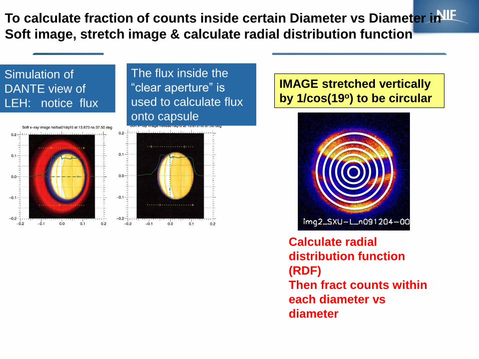
IMAGE stretched vertically

by 1/cos(19o) to be circular

Calculate radial

distribution function

(RDF)

Then fract counts within

each diameter vs

diameter

To calculate fraction of counts inside certain Diameter vs Diameter in

Soft image, stretch image & calculate radial distribution function

Simulation of

DANTE view of

LEH: notice flux

outside of LEH

The flux inside the

“clear aperture” is

used to calculate flux

onto capsule

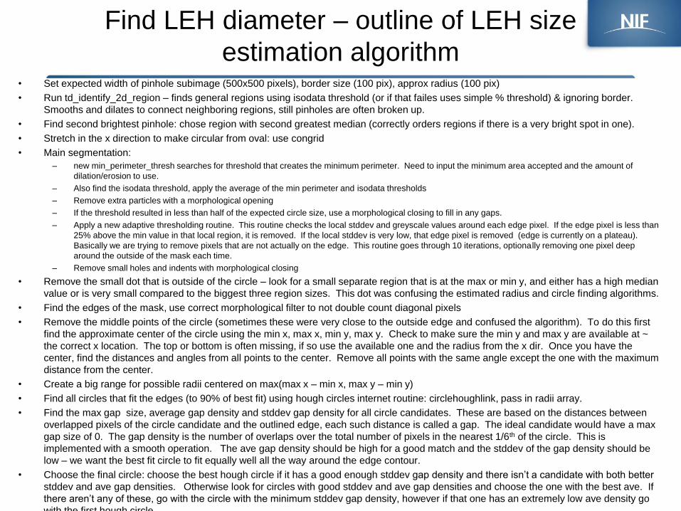
Find LEH diameter – outline of LEH size

estimation algorithm • Set expected width of pinhole subimage (500x500 pixels), border size (100 pix), approx radius (100 pix)

• Run td_identify_2d_region – finds general regions using isodata threshold (or if that failes uses simple % threshold) & ignoring border.

Smooths and dilates to connect neighboring regions, still pinholes are often broken up.

• Find second brightest pinhole: chose region with second greatest median (correctly orders regions if there is a very bright spot in one).

• Stretch in the x direction to make circular from oval: use congrid

• Main segmentation:

– new min_perimeter_thresh searches for threshold that creates the minimum perimeter. Need to input the minimum area accepted and the amount of

dilation/erosion to use.

– Also find the isodata threshold, apply the average of the min perimeter and isodata thresholds

– Remove extra particles with a morphological opening

– If the threshold resulted in less than half of the expected circle size, use a morphological closing to fill in any gaps.

– Apply a new adaptive thresholding routine. This routine checks the local stddev and greyscale values around each edge pixel. If the edge pixel is less than

25% above the min value in that local region, it is removed. If the local stddev is very low, that edge pixel is removed (edge is currently on a plateau).

Basically we are trying to remove pixels that are not actually on the edge. This routine goes through 10 iterations, optionally removing one pixel deep

around the outside of the mask each time.

– Remove small holes and indents with morphological closing

• Remove the small dot that is outside of the circle – look for a small separate region that is at the max or min y, and either has a high median

value or is very small compared to the biggest three region sizes. This dot was confusing the estimated radius and circle finding algorithms.

• Find the edges of the mask, use correct morphological filter to not double count diagonal pixels

• Remove the middle points of the circle (sometimes these were very close to the outside edge and confused the algorithm). To do this first

find the approximate center of the circle using the min x, max x, min y, max y. Check to make sure the min y and max y are available at ~

the correct x location. The top or bottom is often missing, if so use the available one and the radius from the x dir. Once you have the

center, find the distances and angles from all points to the center. Remove all points with the same angle except the one with the maximum

distance from the center.

• Create a big range for possible radii centered on max(max x – min x, max y – min y)

• Find all circles that fit the edges (to 90% of best fit) using hough circles internet routine: circlehoughlink, pass in radii array.

• Find the max gap size, average gap density and stddev gap density for all circle candidates. These are based on the distances between

overlapped pixels of the circle candidate and the outlined edge, each such distance is called a gap. The ideal candidate would have a max

gap size of 0. The gap density is the number of overlaps over the total number of pixels in the nearest 1/6th of the circle. This is

implemented with a smooth operation. The ave gap density should be high for a good match and the stddev of the gap density should be

low – we want the best fit circle to fit equally well all the way around the edge contour.

• Choose the final circle: choose the best hough circle if it has a good enough stddev gap density and there isn’t a candidate with both better

stddev and ave gap densities. Otherwise look for circles with good stddev and ave gap densities and choose the one with the best ave. If

there aren’t any of these, go with the circle with the minimum stddev gap density, however if that one has an extremely low ave density go

with the first hough circle.

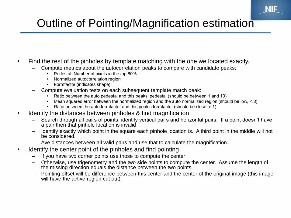
Outline of Pointing/Magnification estimation

• Find the rest of the pinholes by template matching with the one we located exactly. – Compute metrics about the autocorrelation peaks to compare with candidate peaks:

• Pedestal: Number of pixels in the top 80%

• Normalized autocorrelation region

• Formfactor (indicates shape)

– Compute evaluation tests on each subsequent template match peak: • Ratio between the auto pedestal and this peaks’ pedestal (should be between 1 and 10)

• Mean squared error between the normalized region and the auto normalized region (should be low, <.3)

• Ratio between the auto formfactor and this peak’s formfactor (should be close to 1)

• Identify the distances between pinholes & find magnification – Search through all pairs of points, identify vertical pairs and horizontal pairs. If a point doesn’t have

a pair then that pinhole location is invalid

– Identify exactly which point in the square each pinhole location is. A third point in the middle will not be considered.

– Ave distances between all valid pairs and use that to calculate the magnification.

• Identify the center point of the pinholes and find pointing – If you have two corner points use those to compute the center

– Otherwise, use trigenometry and the two side points to compute the center. Assume the length of the missing direction equals the distance between the two points.

– Pointing offset will be difference between this center and the center of the original image (this image will have the active region cut out).

….

….

….

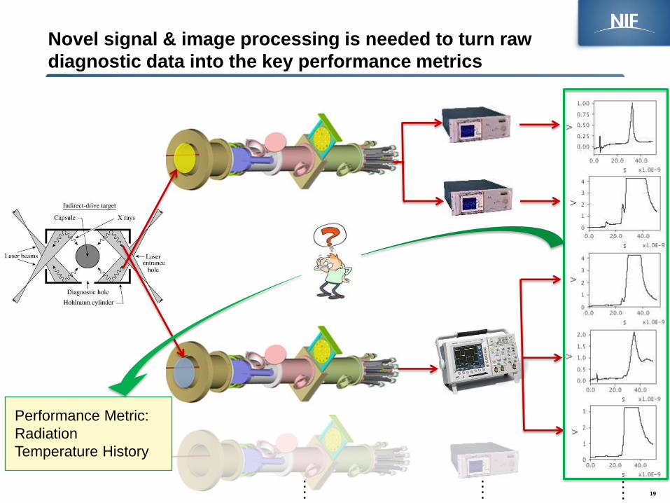
Performance Metric:

Radiation

Temperature History

19

Novel signal & image processing is needed to turn raw

diagnostic data into the key performance metrics

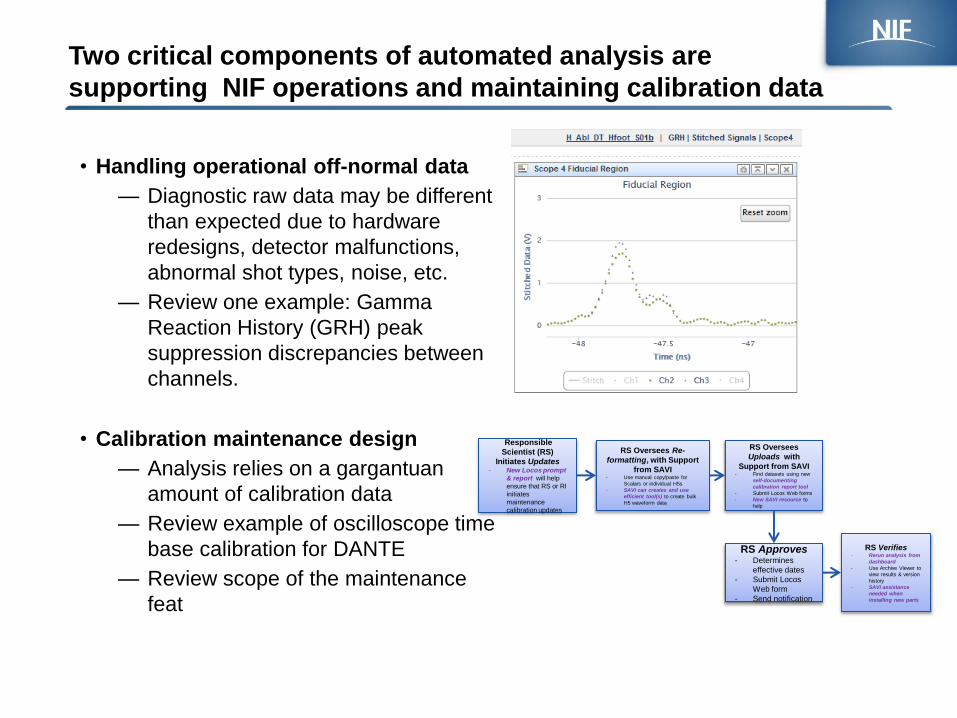
Two critical components of automated analysis are

supporting NIF operations and maintaining calibration data

• Handling operational off-normal data

— Diagnostic raw data may be different

than expected due to hardware

redesigns, detector malfunctions,

abnormal shot types, noise, etc.

— Review one example: Gamma

Reaction History (GRH) peak

suppression discrepancies between

channels.

• Calibration maintenance design

— Analysis relies on a gargantuan

amount of calibration data

— Review example of oscilloscope time

base calibration for DANTE

— Review scope of the maintenance

feat

Responsible

Scientist (RS)

Initiates Updates - New Locos prompt

& report will help

ensure that RS or RI

initiates

maintenance

calibration updates

RS Oversees Re-

formatting, with Support

from SAVI - Use manual copy/paste for

Scalars or individual H5s

- SAVI can creates and use

efficient tool(s) to create bulk

H5 waveform data

RS Oversees

Uploads with

Support from SAVI - Find datasets using new

self-documenting

calibration report tool

- Submit Locos Web forms

- New SAVI resource to

help

RS Approves - Determines

effective dates

- Submit Locos

Web form

- Send notification

RS Verifies - Rerun analysis from

dashboard

- Use Archive Viewer to

view results & version

history

- SAVI assistance

needed when

installing new parts

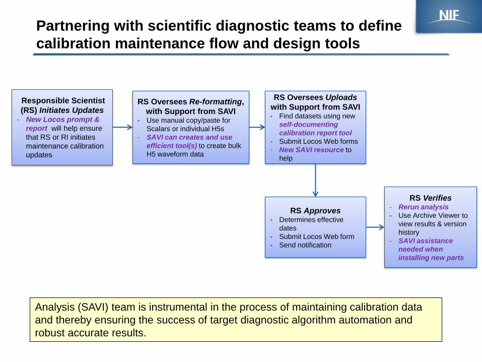
Partnering with scientific diagnostic teams to define

calibration maintenance flow and design tools

Responsible Scientist

(RS) Initiates Updates - New Locos prompt &

report will help ensure

that RS or RI initiates

maintenance calibration

updates

RS Oversees Re-formatting,

with Support from SAVI - Use manual copy/paste for

Scalars or individual H5s

- SAVI can creates and use

efficient tool(s) to create bulk

H5 waveform data

RS Oversees Uploads

with Support from SAVI - Find datasets using new

self-documenting

calibration report tool

- Submit Locos Web forms

- New SAVI resource to

help

RS Approves

- Determines effective

dates

- Submit Locos Web form

- Send notification

RS Verifies - Rerun analysis

- Use Archive Viewer to

view results & version

history

- SAVI assistance

needed when

installing new parts

Analysis (SAVI) team is instrumental in the process of maintaining calibration data

and thereby ensuring the success of target diagnostic algorithm automation and

robust accurate results.

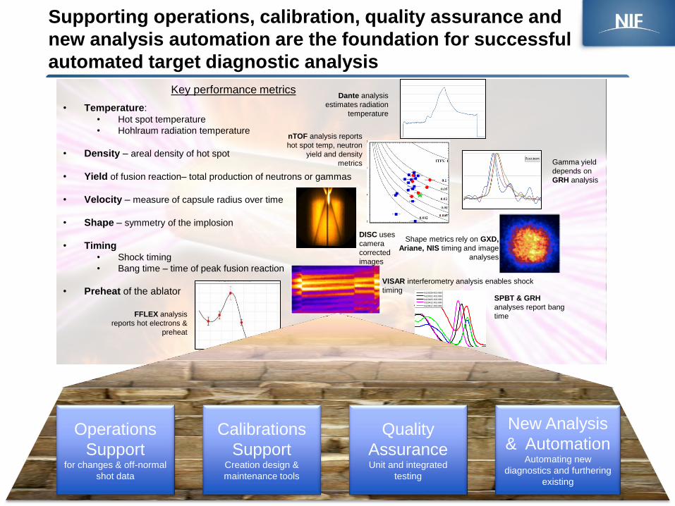
Supporting operations, calibration, quality assurance and

new analysis automation are the foundation for successful

automated target diagnostic analysis

Key performance metrics

• Temperature: • Hot spot temperature

• Hohlraum radiation temperature

• Density – areal density of hot spot

• Yield of fusion reaction– total production of neutrons or gammas

• Velocity – measure of capsule radius over time

• Shape – symmetry of the implosion

• Timing • Shock timing

• Bang time – time of peak fusion reaction

• Preheat of the ablator

VISAR interferometry analysis enables shock

timing

FFLEX analysis

reports hot electrons &

preheat

21.5 22 22.5 23 23.50

5

10

15

20

25

30

Time (ns)

Deconv. S

ignal (V

)

SPBT

N120329-001-999

N120321-001-999

N120405-003-999

N120412-001-999

N120417-002-999

SPBT & GRH

analyses report bang

time

DISC uses

camera

corrected

images

Shape metrics rely on GXD,

Ariane, NIS timing and image

analyses

Dante analysis

estimates radiation

temperature

Gamma yield

depends on

GRH analysis

nTOF analysis reports

hot spot temp, neutron

yield and density

metrics

22

Operations

Support for changes & off-normal

shot data

Calibrations

Support Creation design &

maintenance tools

Quality

Assurance Unit and integrated

testing

New Analysis

& Automation Automating new

diagnostics and furthering

existing