arX

iv:h

ep-p

h/94

0322

7 v1

4

Mar

199

4

NIKHEF-94-P1, hep-ph/9403227

Intrinsic transverse momentum

and the polarized Drell-Yan process

R.D. Tangerman and P.J. Mulders∗

National Institute for Nuclear Physics and High Energy Physics (NIKHEF-K),

P.O. Box 41882, NL-1009 DB Amsterdam, The Netherlands

(March 1994, revised August 1994)

Abstract

In this paper we study the cross section at leading order in 1/Q for polarized

Drell-Yan scattering at measured lepton-pair transverse momentum QT . We

find that for a hadron with spin 1/2 the quark content at leading order is

described by six distribution functions for each flavor, which depend on both

the lightcone momentum fraction x, and the quark transverse momentum k2T .

These functions are illustrated for a free-quark ensemble. The cross sections

for both longitudinal and transverse polarizations are expressed in terms of

convolution integrals over the distribution functions.

PACS numbers: 13.85.Qk, 13.88.+e

Typeset using REVTEX

∗Also at Physics Department, Free University, NL-1081 HV Amsterdam, The Netherlands.

1

I. INTRODUCTION

The measurements of unpolarized structure functions in deep inelastic scattering (DIS)of leptons off nucleons and nuclei and those of polarized structure functions in scatteringof longitudinally polarized electrons off longitudinally polarized nucleons [1] have yieldedthe lightcone momentum distributions f1(x) for quarks in various targets and the helicitydistributions g1(x) in protons and neutrons1. These measurements, and particularly theirinterpretation, have shown the importance of understanding the relation of these distri-butions to the structure of the target. The distributions f1(x) and g1(x) characterize theresponse of the hadron in inclusive DIS at leading order in the transferred momentum Q.In inclusive deep inelastic lepton-hadron (ℓH) scattering the quark transverse momentumis not observable, since it is integrated over. In the Drell-Yan (DY) process at measuredlepton-pair transverse momentum QT , however, quark transverse momentum does enter inobservables, notably in the angular distribution of the lepton pairs. The main point of thispaper is the discussion of quark transverse momentum in polarized Drell-Yan scattering. Wewill restrict ourselves to leading order and discard contributions which are suppressed byorders of 1/Q. We will also not discuss QCD radiative corrections, giving rise to logarithmiccorrections.

For inclusive deep inelastic ℓH scattering, assuming only one flavor, the hadron tensoris given as the imaginary part of the forward virtual Compton amplitude, for large virtualphoton momentum q (Q2 ≡ −q2 large) given by the sum of the quark and antiquark handbagdiagrams of Fig. 1. The basic object, encoding the soft physics of the quarks inside thehadron, is the correlation function [2,3]

Φij(PS; k) =∫

d4x

(2π)4eik·x〈PS|ψj(0)ψi(x)|PS〉c, (1.1)

where k is the momentum of the quark. The vectors P and S are the momentum andspin vector of the target hadron. Evaluating the hard part, the scattering of the virtualphoton off the quarks, it turns out that the structure functions in the cross section becomeproportional to f1(xbj) and g1(xbj), where xbj = Q2/2P · q. The function f1 is given by

f1(x) =1

2

∫

dk−d2kT Tr[

γ+Φ(PS; k)]

, (1.2)

where x = k+/P+. It can be interpreted as the longitudinal (lightcone) momentum distri-bution of quarks. The function g1 appears as

λ g1(x) =1

2

∫

dk−d2kT Tr[

γ+γ5Φ(PS; k)]

, (1.3)

and can be interpreted as the quark helicity distribution in a longitudinally polarized nucleon(helicity λ = 1). The functions f1 and g1 are specific projections of Φ. Which projections of

1Another often used notation is q(x) for the lightcone momentum distribution and ∆q(x) for the

helicity distribution (q = u, d, s, . . .).

2

Φ contribute in hard scattering processes in leading order can be investigated by looking atthe operator structure, including the Dirac and Lorentz structure, of the correlation function.Such an analysis requires some physical constraints on the range of quark momenta. Theanalysis of Φ (integrated over k− and kT ) shows that there is one more leading function, thetransverse polarization or transversity2 distribution h1. It is related to a bilocal quark-quarkmatrix element through [6]

SiT h1(x) =

1

2

∫

dk−d2kT Tr[

iσi+γ5Φ(PS; k)]

(i = 1, 2), (1.4)

which shows that h1 can be interpreted as the quark transversity distribution in a trans-versely polarized nucleon. This is a chiral-odd distribution, which is not observable ininclusive ℓH scattering. It needs to be combined with some other chiral-odd structure,e.g., the fragmentation part in semi-inclusive leptoproduction of hadrons or the antiquarkdistribution part of DY scattering [4,5,7,8].

In this paper we discuss one possible way to extract more information from the cor-relation function Φ. We are after the dependence on the transverse momentum kT . Oneway to study this dependence is the observation of a hadron in the outgoing quark jet, e.g.,in semi-inclusive ℓH scattering [9]. This process, however, also requires consideration ofthe fragmentation functions. In this paper we study the process that is sensitive to intrin-sic transverse momentum and involves only quark distribution functions, namely, massivedilepton production or the Drell-Yan (DY) process [10].

About fifteen years ago Ralston and Soper (RS) published a pioneering paper [6] on thepolarized Drell-Yan process. Because we take it as our starting point, we briefly sketch itscontent. RS write down a covariant expansion for

∫

dk−Φ, which is the quantity that isrelevant in the hadron tensor for the DY process. To determine this expansion they usesymmetry arguments and an infinite-momentum-frame analysis. They find five independentdistribution functions, divided in one momentum probability distribution P(x,k2

T ), twofunctions describing the quark helicity, and two describing its transverse polarization. Withthese they calculate the polarized Drell-Yan cross section with the virtual photon transverse

momentum QT ≡√

q2T put to zero. In that case they are sensitive to four of the five

distribution functions. When they integrate over the transverse momentum they are onlysensitive to three distribution functions.

We extend on these results in two ways. First, we show that RS left out one transversemomentum distribution, needed to describe the quark transverse polarization. This addi-tional function is obtained using general symmetry arguments. It also shows up in a modelthat we are going to employ later and that describes a gas of free partons. Our secondextension is the calculation of the polarized DY cross section without constraints on QT

[other than it being of O(Λ)], thereby becoming sensitive to all six distribution functions.

2The authors of [4] use the name ‘transversity distribution’ in order to make clear that a quark of

definite transversity is not in an eigenstate of the transverse spin operator but of the Pauli-Lubanski

operator projected along a transverse direction. The authors of [5] object to this nomenclature,

because of the pre-existence of the term, and prefer to call it transverse polarization distribution.

3

We end this introduction with a remark on possible QCD corrections affecting transversemomenta and factorization. A difficulty of the extra scale QT is the Sudakov effect. Softgluon radiation gives rise to radiative transverse momentum. However, the large logarithmsconnected with this effect can be summed and exponentiated to Sudakov form factors [11].From these it becomes clear that if QT is sufficiently low, i.e., of hadronic scale Λ, as com-pared to Q, the transverse momentum governing the process is predominantly intrinsic.Factorization means that the process can be written as a convolution of renormalized distri-bution functions and a perturbatively calculable short-distance part. For polarized DY atmeasured QT

<∼ Λ factorization has not been proven yet [12,13]. We will not further addressthis problem here, but use the diagrammatic expansion proposed by Ellis, Furmanski, andPetronzio (EFP) [14] to study the DY process. In this diagrammatic expansion Green func-tions appear, incorporating the long-range QCD physics. These correlation functions areconnected by ordinary Feynman graphs with quarks and gluons, the hard scattering piece.

The outline of this paper is as follows. In Sec. II we give the one-photon exchangepicture for massive dilepton production. We specify the notation in a frame where thetwo hadrons are collinear, and the axes are given with respect to which the lepton anglesare defined. In Sec. III we analyze the quark correlation function, and find six leadingdistribution functions. In Sec. IV we discuss the free-quark ensemble as an example. InSec. V we calculate the leading-order hadron tensor and present cross sections for variouscombinations of polarizations. We end with a discussion of these results.

II. THE DRELL-YAN PROCESS

In this section we want to discuss the cross section, kinematic aspects, and structurefunctions, for polarized Drell-Yan scattering. For a complete overview we refer for theunpolarized process to Lam and Tung [15], and for polarized DY scattering to Donohue andGottlieb [16], who make use of the Jackob-Wick helicity formalism.

A. The DY cross section

We consider the process A + B → ℓ + ℓ +X, where two spin-12

hadrons with momentaP µ

A and P µB interact and two outgoing leptons are measured with momenta kµ

1 and kµ2 . The

leptons are assumed to originate from a high-mass photon with momentum q = k1+k2, withQ2 ≡ q2 > 0. We consider the case of pure incoming spin states, characterized by the spinvectors Sµ

A and SµB, i.e., S2

A = S2B = −1. In the deep inelastic limit Q2 and s = (PA + PB)2

become large compared to the characteristic hadronic scale of order Λ2 ∼ 0.1 GeV2, whiletheir ratio τ = Q2/s is fixed. The phase space element for the lepton pair can be written asd4q dΩ, where the angles are those of the lepton axis in the dilepton rest frame with respectto a suitably chosen Cartesian set of axes. The cross section can be written as

dσ

d4qdΩ=

α2

2sQ4LµνW

µν , (2.1)

where the lepton tensor is given by (neglecting the lepton masses)

Lµν = 2 kµ1k

ν2 + 2 kµ

2kν1 −Q2 gµν , (2.2)

4

and the hadron tensor can be written as

W µν(q;PASA;PBSB) =∫

d4x

(2π)4eiq·x〈PASA;PBSB| [Jµ(0), Jν(x)] |PASA;PBSB〉. (2.3)

Since the lepton tensor (2.2) is symmetric in its indices, we will from now on only considerthe symmetric part of W µν .

B. Kinematics

We define the transverse momentum of the produced lepton pair in a frame where thehadrons are collinear, with the third axis chosen along the direction of hadron A. Onehas q2

T ≡ Q2T<∼ Λ2. It is convenient to work in a lightcone component representation,

p = [p−, p+,pT ] with p± ≡ (p0 ± p3)/√

2. The momenta of the hadrons and the virtualphoton in a collinear frame take the form

PA =

[

M2A

2P+A

, P+A , 0T

]

≈[

xAM2A√

2κQ,κQ√2 xA

, 0T

]

, (2.4)

PB =

[

P−B ,

M2B

2P−B

, 0T

]

≈[

Q√2κxB

,κxBM

2B√

2Q, 0T

]

, (2.5)

q =[

xBP−B , xAP

+A , qT

]

≈[

Q√2κ

,κQ√

2, qT

]

, (2.6)

neglecting corrections of order 1/Q2, indicated here and further on by an approximate equal.The parameter κ fixes the collinear frame. One has κ = xAMA/Q for the frame in which

hadron A is at rest, κ =√

xA/xB for the hadron center-of-mass frame, and κ = Q/xBMB

for the frame in which hadron B is at rest. The following Lorentz-invariant relations hold:

xA =q+

P+A

≈ Q2

2PA · q ≈ PB · qPB · PA

, (2.7)

xB =q−

P−B

≈ Q2

2PB · q ≈ PA · qPA · PB

, (2.8)

s ≈ 2P+A P

−B ≈ Q2

xAxB. (2.9)

The above relations also show that all dot products for any pair from the vectors q, PA, andPB, are of order Q2. As compared to this, the hadron momenta are almost lightlike. Wecan define the exactly lightlike vectors that in a given collinear frame have the form

n+ ≡ [0, κ, 0T ],

n− ≡ [κ−1, 0, 0T ], (2.10)

satisfying n+ · n− = 1. Given an arbitrary four-vector a, and the projector

gµνT ≡ gµν − nµ

+nν− − nν

+nµ−, (2.11)

5

we define the spacelike transverse four-vector aµT ≡ gµν

T aν , or, in coordinates in a collinearframe, aT = [0, 0,aT ]. Note that for any transverse vector one has

aT · PA = aT · PB = 0. (2.12)

For the analysis of the hadronic tensor which satisfies qµWµν = qν Wµν = 0, it is impor-tant to construct vectors that are orthogonal to q. We will use the projector

gµν ≡ gµν − qµqν

q2(2.13)

for this, and define

aµ ≡ gµνaν = aµ − a · qq2

qµ. (2.14)

As q is timelike in DY scattering, it is useful to define a set of Cartesian axes. The Z-direction, known as the Collins-Soper axis [17], is chosen as in [6], but ourX- and Y -directionare opposite. To be precise, we use (ǫ0123 = 1)

Zµ ≡ PB · qPB · PA

P µA − PA · q

PA · PBP µ

B =PB · qPB · PA

P µA − PA · q

PA · PBP µ

B,

Xµ ≡ − PB · ZPB · PA

P µA +

PA · ZPA · PB

P µB, (2.15)

Y µ ≡ 1

PA · PBǫµνρσPAνPBρqσ.

These vectors are orthogonal and satisfy Z2 ≈ −Q2 and X2 ≈ Y 2 ≈ q2T = −Q2

T . They forma natural set of spacelike axes (with in the dilepton rest frame only spatial components). Wewill denote qµ = qµ/Q, zµ = Zµ/

√−Z2, etcetera. Explicitly, one has in a collinear frame

q ≈[

1√2 κ

,κ√2,qT

Q

]

,

z ≈[

− 1√2κ

,κ√2, 0T

]

,

x ≈[

1√2 κ

QT

Q,κ√2

QT

Q,qT

QT

]

, (2.16)

y ≈[

0, 0,yT

QT

]

,

where yiT = ǫijqTj. Note that since Zµ is a linear combination of the hadron momenta,

it has in collinear frames no transverse components. The transverse vectors aT , thus, areorthogonal to Z. They are, in general, not orthogonal to q. One has, for example, qµ

T ≈Xµ−(Q2

T /Q2) qµ. Note that the second term is only order 1/Q suppressed. For an arbitrary

four-vector a we define the perpendicular four-vector a⊥ as the projection of the transversevector aT , using the projector

gµν⊥ ≡ gµν − qµqν + zµzν , (2.17)

6

yielding

aµ⊥ ≡ gµν

⊥ aTν = aµT − q · aT

q2qµ. (2.18)

Thus, any perpendicular vector satisfies

a⊥ · q = a⊥ · z = 0. (2.19)

Note that X is the perpendicular projection of q. The vectors n+ and n−, defined inEq. (2.10), can be expressed in terms of the set (2.16),

n+ ≈ 1√2

(

q + z − QT

Qx

)

,

n− ≈ 1√2

(

q − z − QT

Qx

)

, (2.20)

Inserting these into the definitions of the projectors g⊥ and gT , one derives the relation

gµν⊥ ≈ gµν

T − (qµqνT + qνqµ

T )

Q, (2.21)

from which one obtains for a general vector a:

aµ⊥ ≈ aµ

T − aT · qTQ

qµ, (2.22)

provided that aT · qT = O(1). From this expression it is evident that for two arbitraryvectors a and b, satisfying this condition,

a⊥ · b⊥ ≈ aT · bT . (2.23)

Restricting oneself to leading order, the vectors aT and a⊥ can be freely interchanged. In ahigher order study, however, the difference will become important [18].

For the spin vectors the above definitions can be illustrated. In a collinear frame thespin vectors, satisfying PA · SA = PB · SB = 0, can be written as

SA =

[

−λAMA

2P+A

, λAP+

A

MA

,SAT

]

, (2.24)

SB =

[

λBP−

B

MB,−λB

MB

2P−B

,SBT

]

. (2.25)

where λA, and λB, are the hadron helicities. The two-component vectors SAT , and SBT ,give the transverse polarization. Since we consider pure spin states, they obey λ2 + S2

T = 1.For the spin vectors we have in a collinear frame ST = [0, 0,ST ]. The perpendicular spinvector is given by

Sµ⊥ ≈ Sµ

T − ST · qTQ

qµ =

[

O(

1

κQ

)

,O(

κ

Q

)

,ST + O(

1

Q2

)]

, (2.26)

7

where the longitudinal components follow from the transverse components by demandingEq. (2.19), and using Eq. (2.16). If the spin vector would have been projected directly ontothe XY -plane with gµν

⊥ , one would have got

gµν⊥ Sν =

[

O(

1

κQ

)

,O(

κ

Q

)

,ST − λ

2 xMqT + O

(

1

Q2

)]

. (2.27)

This differs from ST in the transverse sector by O(1), unless QT = 0.

C. Structure functions

With the definition (2.15) of a Cartesian set of vectors orthogonal to q, we can expandthe lepton momenta in the following way:

kµ1 = 1

2qµ + 1

2Q(sin θ cos φ xµ + sin θ sin φ yµ + cos θ zµ),

kµ2 = 1

2qµ − 1

2Q(sin θ cosφ xµ + sin θ sinφ yµ + cos θ zµ). (2.28)

Inserting these into Eq. (2.2), and using some trivial goniometric relations and the com-pleteness relation gµν = qµqν − zµzν − xµxν − yµyν , we obtain

Lµν = −Q2

2

[

(1 + cos2 θ) gµν⊥ − 2 sin2 θ zµzν + 2 sin2 θ cos 2φ (xµxν + 1

2gµν⊥ )

+ sin2 θ sin 2φ xµyν + sin 2θ cosφ zµxν + sin 2θ sin φ zµyν]

, (2.29)

where the symmetrization of indices, zµxν ≡ zµxν + zν xµ, is used. The six tensor com-binations in Eq. (2.29) are not only orthogonal to q, ensuring qµL

µν = 0, but also to eachother.

It is convenient also to write the hadron tensor as a sum of products of tensors and scalarfunctions, called structure functions. From the properties of the electromagnetic current,one deduces for the hadronic tensor [Eq. (2.3)] the following conditions:

qµWµν = 0 [Current conservation]

[W νµ]∗ = W µν [Hermiticity]Wµν(q; PA −SA; PB −SB) = W µν(q;PASA;PBSB) [Parity]Wµν(q; PASA; PBSB) = [W µν(q;PASA;PBSB)]∗ [Time reversal]

(2.30)

where aµ ≡ aµ. The hermiticity condition, for instance, requires that the symmetric part ofW µν is real. In unpolarized scattering the constraints imply the expansion

W µν = −(W0,0 − 13W2,0) g

µν⊥ + (W0,0 + 2

3W2,0) z

µzν −W2,1 zµxν −W2,2 (xµxν + 1

2gµν⊥ ),

(2.31)

where the four structure functions depend on the (four) independent scalars, or equivalentlyon Q, xA, xB, and QT . Since we choose to work with the normalized vectors, the structurefunctions W2,1 and W2,2 contain kinematical zeros for X2 ≈ −Q2

T = 0 of first and secondorder, respectively. In that they differ from the ones in RS [6, Eq. (2.5)]. To be precise:

8

our W2,1 is√X2Z2 times theirs, and our W2,2 is −X2 times theirs. The linear combinations

multiplying −gµν⊥ and zµzν are often referred to as WT and WL, respectively. Inserting

Eqs. (2.29) and (2.31) into Eq. (2.1), one has for unpolarized Drell-Yan scattering

dσ

d4qdΩ=

α2

2sQ2

[

2W0,0 +W2,0 (13− cos2 θ) +W2,1 sin 2θ cosφ+W2,2

12sin2 θ cos 2φ

]

. (2.32)

Due to the extra pseudo-vectors SA and SB, in polarized Drell-Yan there are several morestructure functions. We will not give them in general. Later we will simply consider theones that arise at leading order in 1/Q in the cross section.

III. FORMALISM

A. The correlation function

In order to calculate the hadron tensor, the diagrammatic expansion of EFP is used [14].Each diagram is composed of soft nonlocal matrix elements, convoluted with a hard cut-amplitude. For example, in DY scattering the simplest diagrams (Born diagrams) are givenin Fig. 2. The nonlocal matrix element describing the nonperturbative long-range physicsfor a quark of flavor a inside hadron A, is given by the quark-quark correlation function

(Φa/A)ij(PASA; k) =∫ d4x

(2π)4eik·x〈PASA|ψ

(a)

j (0)ψ(a)i (x)|PASA〉c, (3.1)

diagrammatically represented in Fig. 3. We will suppress the quark label a, the hadronlabel A, and the connectedness subscript c, whenever they are not explicitly needed. Acontraction over color indices is implicit. More general, the correlation functions contain anumber of quark and gluon fields, but at lowest order in 1/Q only the one above is relevant.

A point that needs to be mentioned is the color gauge invariance of the correlationfunction defined above. For a proper gauge-invariant definition of a nonlocal matrix elementa color link operator, L(0, x) = P exp[ig

∫ x0 ds · A(s)], must be inserted. As will be seen

below, we only need the integral of Φ over k−, i.e., the nonlocality is restricted to the planex+ = 0. Going further and integrating also over transverse momenta, one is only sensitiveto the nonlocality in a lightlike direction (say x−). With an appropriate choice of path (astraight link) and lightcone gauge (A+ = 0), the link operator becomes just unity. Whentransverse momentum is observed, this no longer is the case, since one becomes sensitiveto transverse separation xT , although still x+ = 0. Fixing the residual gauge freedom thataffects AT can be achieved by imposing boundary conditions [19]. A path from 0 to x canthen be constructed such that the link operator becomes unity after gauge-fixing. How thechoices of gauge and path connect to the proof of factorization remains an open question.

B. The Dirac structure of the correlation function

In order to analyze the diagrams in Fig. 2 for DY scattering, we need to investigate theDirac structure of the correlation function. This can be done by making an expansion in

9

an appropriate basis. Constraints on the correlation function come from hermiticity, parityinvariance, and time reversal invariance,

Φ†(PS; k) = γ0 Φ(PS; k) γ0 [Hermiticity]Φ(PS; k) = γ0 Φ(P −S; k) γ0 [Parity]Φ∗(PS; k) = γ5C Φ(P S; k)C†γ5 [Time reversal]

(3.2)

where the charge conjugation matrix C = iγ2γ0, and kµ = kµ. Choosing the Dirac matrixbasis 1, iγ5, γ

µ, γµγ5, and iσµνγ5 (note that Γ† = γ0Γγ0), the most general structuresatisfying these constraints is

Φ(PS; k) = A1 1 + A2 6P + A3 6k+A4 γ5 6S + A5 γ5[6P , 6S] + A6 γ5[6k, 6S]

+A7 k · S γ5 6P + A8 k · S γ5 6k + A9 k · S γ5[6P , 6k]. (3.3)

Hermiticity requires all the amplitudes Ai = Ai(k · P, k2) to be real. Note the presence ofthe amplitude A9 which is left out in Eq. (3.4) of Ref. [6].

The basic assumption made for the correlation function is that in the hadron rest framethe quark momentum k is restricted to a hadronic scale Λ, explicitly k2 and k · P are ofO(Λ2). In a frame where the hadron has no transverse momentum, the momentum k iswritten as

k =

[

k2 + k2T

2xP+, x P+,kT

]

, (3.4)

with the lightcone momentum fraction x = k+/P+. The restrictions on k2 and k · P implythat also k2

T = −k2 + 2xk · P − x2M2 is of O(Λ2). Considering diagram 2a, one seeseasily that momentum conservation on the hard vertex implies q− = k−a + k−b . However,k−b ∼ P−

B , whereas k−a ∼M2A/P

+A , which is down by a factor ∼ M2/Q2 in any collinear frame.

Therefore, for hadron A, one is led to study∫

dk− Φ(PS; k), or equivalently its projections∫

dk− Tr[ΓΦ]. These latter quantities do not carry Dirac indices anymore, but because ofthe Γ-matrices, they do have a specific Lorentz tensor character. Defining the projections

Φ[Γ](x,kT ) ≡ 1

2

∫

dk− Tr [Γ Φ] (3.5)

=1

2

∫

dx−

2π

d2xT

(2π)2exp[i(xP+x− − kT · xT )] 〈PS|ψ(0)Γψ(0, x−,xT )|PS〉, (3.6)

one has for instance the vector projection

Φ[γ+] =∫

d(2k · P )dk2 δ(

k2T + k2 − 2xk · P + x2M2

)

(A2 + xA3), (3.7)

which is O(1). Other projections, e.g., the scalar

Φ[1] =1

P+

∫

d(2k · P )dk2 δ(

k2T + k2 − 2xk · P + x2M2

)

A1, (3.8)

contain an integral of O(1) multiplied by a factor 1/P+. In the cross section, this factor willgive rise to a suppression of order 1/Q. In this way it is seen that the leading contributions

10

come from the Dirac structure where the number of +-components minus the number of−-components is largest (that is, 1). They are parametrized as

Φ[γ+] = f1(x,k2T ),

Φ[γ+γ5] = g1L(x,k2T )λ+ g1T (x,k2

T )kT · ST

M, (3.9)

Φ[iσi+γ5] = h1T (x,k2T )Si

T +

[

h⊥1L(x,k2T )λ+ h⊥1T (x,k2

T )kT · ST

M

]

kiT

M,

defining six real distribution functions per flavor, depending on x and k2T . These encode the

leading behavior of the quark correlation function. An expansion can be made in terms oflocal operators which have twist two and higher.

In the diagrammatic expansion for the DY hadron tensor (with A+ = 0 for the lowerblob), correlations will appear with, in addition to the quark fields, transverse gluon fieldsin the soft part, ψ(0)Aα

T (y)ψ(x), etc.. They can be analyzed in the same way, and turn outto be suppressed by one order of 1/Q for each additional gluon field.

In summary, for a leading-order DY calculation, one is to use∫

dk−Φ = 12Φ[γ+] γ− + 1

2Φ[γ+γ5] γ5γ

− + 12Φ[iσi+γ5] iγ5σ

−i + . . . , (3.10)

where i is a transverse index (i.e., i = 1, 2), and the dots represent projections that willcome in only at O(1/Q). At the leading-order level, one is left with only three projections,which have vector, axial-vector, and axial-tensor character, respectively, and which can beparametrized by six distribution functions.

C. Antiquarks

The antiquark correlation function, describing the antiquarks of flavor a, is given by(contracting over color indices)

(Φa/A)ij(PASA; k) =∫

d4x

(2π)4eik·x〈PASA|ψ(a)

i (0)ψ(a)

j (x)|PASA〉c. (3.11)

Also the antiquark momentum k can be written as in Eq. (3.4). Its Dirac structure can beanalyzed likewise. We define the antiquark projections

Φ[Γ](x,kT ) ≡ 1

2

∫

dk− Tr[

Γ Φ]

(3.12)

=1

2

∫

dx−

2π

d2xT

(2π)2exp[i(xP+x− − kT · xT )] 〈PS|Tr

[

Γψ(0)ψ(0, x−,xT )]

|PS〉. (3.13)

Using the charge conjugation properties of Dirac fields and hadron states, we deduce

Φa/A = −C−1(

Φa/A

)TC. (3.14)

Upon demanding charge conjugation invariance of the distribution functions, i.e., the quarkdistributions in the antihadron A are the same as the corresponding antiquark distributionsin A, we obtain the expressions

11

Φ[γ+] = f1(x,k2T ), (3.15)

Φ[γ+γ5] = −g1L(x,k2T )λ− g1T (x,k2

T )kT · ST

M, (3.16)

Φ[iσi+γ5] = h1T (x,k2T )Si

T +

[

h⊥1L(x,k2T )λ+ h⊥1T (x,k2

T )kT · ST

M

]

kiT

M. (3.17)

We note that the anticommutation relations for fermions can be used to obtain thesymmetry relation

Φij(PS; k) = −Φij(PS;−k). (3.18)

For the distribution functions this gives the symmetry relation

f1(x,k2T ) = −f1(−x,k2

T ), (3.19)

and identically for g1T , h1T and h⊥1T , whereas

g1L(x,k2T ) = g1L(−x,k2

T ), (3.20)

and identically for h⊥1L

Finally, we note that hadron B can be treated in the same fashion. However, since wehave chosen to work in the collinear frames where the third axis lies opposite to the directionof hadron B, the role of the +- and −-components for B must be interchanged as comparedto A. So, in Fig. 2a the upper blob reduces to

∫

dk+b Φ(PBSB; kb), for which one has to use

the gauge A− = 0.

IV. FREE-QUARK ENSEMBLE

The leading kT -integrated distributions f1(x), g1(x), and h1(x), have a parton modelinterpretation as the longitudinal momentum, helicity, and transversity distribution, respec-tively. In this section we show how, for a free-quark ensemble, this identification can begeneralized to the kT -dependent distributions.

It is instructive to calculate the correlation function for a free-quark target of flavor a.This is given by

(Φa/a)ij(p s; k) = δ4(k − p) ui(p, s)uj(p, s) = δ4(k − p)

[

( 6k +m)

(

1 + γ5 6s2

)]

ij

, (4.1)

where the momentum and spin vector are parametrized as

k =

[

m2 + k2T

2k+, k+,kT

]

, (4.2)

s = λank + sat = λa

[

k2T −m2

2mk+,k+

m,kT

m

]

+

[

kT · saT

k+, 0, saT

]

. (4.3)

We identify the lightcone helicity λa, helicity vector nk, and transverse polarization sat

(transverse in the sense that sat · k = sat · nk = 0). Note that the lightcone helicity vector

12

nk, satisfying nk · k = 0 and n2k = −1, acquires its conventional meaning [20, Eq. (2-49)],

either if kT = 0T , or in the infinite-momentum-limit k+ → ∞ with kT fixed. One checksthat λ2

a + s2aT = −s2 = 1. With the simple form (4.1) it is straightforward to calculate the

leading projections for a free-quark target with non-zero transverse momentum,

1

2

∫

dk− Tr[γ+Φ(p s; k)] = δ

(

k+

p+− 1

)

δ2(kT − pT ),

1

2

∫

dk− Tr[γ+γ5Φ(p s; k)] = δ

(

k+

p+− 1

)

δ2(kT − pT )λa, (4.4)

1

2

∫

dk− Tr[iσi+γ5Φ(p s; k)] = δ

(

k+

p+− 1

)

δ2(kT − pT ) siaT .

This simple example of a quark target can be generalized to the case in which thehadron is considered as a beam of non-interacting partons of total momentum P and angularmomentum S. This is tantamount to inserting free-field plane-wave expansions into thecorrelation function (3.1). One gets (summing over α, β = 1, 2)

Φij(PS; k) = 2 δ(k2 −m2)[

θ(k+)u(β)i (k)Pβα(k)u

(α)j (k) − θ(−k+)v

(β)i (−k)Pβα(−k)v(α)

j (−k)]

.

(4.5)

The functions P and P are given by

Pβα(k) = Pβα(x,kT ) ≡ 1

2(2π)3

∫

dx′ d2k′T

(2π)3 2x′〈PS|b†α(k′)bβ(k)|PS〉, (4.6)

Pβα(k) = Pβα(x,kT ) ≡ 1

2(2π)3

∫

dx′ d2k′T

(2π)3 2x′〈PS|d†β(k′)dα(k)|PS〉. (4.7)

The form of quantization one can choose to be instant-front, as well as light-front quantiza-tion, since for free fields they are equivalent [19]. As for the choice of coordinates, the useof lightcone coordinates is convenient, because of the integration over k− that is needed indeep inelastic processes. The Dirac structure can be parametrized as

u(β)(k)Pβα(k)u(α)(k) = P(k)( 6k +m)

(

1 + γ5 6s(k)2

)

, (4.8)

v(β)(k)Pβα(k)v(α)(k) = P(k)( 6k −m)

(

1 + γ5 6s(k)2

)

, (4.9)

in terms of positive definite quark and antiquark probability densities P(k) and P(k), andspin vectors sµ(k) and sµ(k) . Inserting the free-field expansion in the current expecta-tion value 〈PS|ψ(0)γµψ(0)|PS〉 = 2P µ(N − N), where N and N are the total number ofquarks and antiquarks, respectively, one obtains from the +-component the normalizations∫ 10 dx

∫

d2kTP(x,k2T ) = N and

∫ 10 dx

∫

d2kTP(x,k2T ) = N . The average quark spin vector

sµ(k) is parametrized by the helicity density λa(x,kT ) and transverse polarization densitysaT (x,kT ) by expanding sµ as in Eq. (4.3). A similar parametrization is used for sµ(k) interms of λa(x,kT ) and saT (x,kT ).

13

Integrating Eq. (4.5) over k− one obtains the result for a free-quark ensemble,

1

2

∫

dk−Φ(k) = θ(x)P(x,k2

T )

2k+( 6k +m)

(

1 + γ5 6s(x,kT )

2

)

− θ(−x)P(−x,k2T )

2k+( 6k +m)

(

1 + γ5 6s(−x,−kT )

2

)

. (4.10)

This gives (for x > 0)

1

2

∫

dk− Tr[γ+Φ(PS; k)] = P(x,k2T ),

1

2

∫

dk− Tr[γ+γ5Φ(PS; k)] = P(x,k2T )λa(x,kT ), (4.11)

1

2

∫

dk− Tr[iσi+γ5Φ(PS; k)] = P(x,k2T ) si

aT (x,kT ).

A comparison with Eq. (3.9) yields

P(x,k2T ) = f(x,k2

T ),

P(x,k2T )λa(x,kT ) = g1L(x,k2

T )λ+ g1T (x,k2T )

kT · ST

M, (4.12)

P(x,k2T ) si

aT (x,kT ) = h1T (x,k2T ) Si

T +

[

h⊥1L(x,k2T )λ+ h⊥1T (x,k2

T )kT · ST

M

]

kiT

M,

which shows how for x > 0 the functions g1L, g1T , h1T , h⊥1L, and h⊥1T , are to be inter-preted as quark longitudinal and transverse polarization distributions. The function h⊥1T

was omitted in the paper of RS. Specifically for non-zero transverse momenta of the quarks,it becomes relevant. For the antiquarks the same relations hold between the antiquarkprobability density P, helicity density λa, and transverse polarization density saT , on theone hand, and the antiquark distributions on the other hand. Extending to all x, re-sults are obtained in accordance with the symmetry relations in the previous section, e.g.,f(x,k2

T ) = θ(x)P(x,k2T ) − θ(−x)P(−x,k2

T ). For on-shell quarks, relations exist betweenthe distributions due to constraints from Lorentz invariance [14]. The scalar P can onlydepend on 2k · P = m2/x +M2x + k2

T/x and the pseudovector sµ can be parametrized bytwo functions depending on the same combination of x and k2

T .We note that for the leading-order matrix elements the free-field results can be used

to provide a parton interpretation, even in the interacting theory, because the distributionfunctions can be expressed as densities for specific projections of the so-called ‘good’ com-ponents of the quark field; ψ+ ≡ Λ+ψ, where Λ+ = 1

2γ−γ+. In light-front quantization a

Fourier expansion for the good components (at x+ = 0) can be written down in which theFourier coefficients can be interpreted as particle and antiparticle creation and annihilationoperators [19]. The different polarization distributions involve projection operators thatcommute with Λ+ [4].

At subleading order, the analysis of the quark-quark correlation functions leads to anumber of new distribution functions. For free quarks, they can also be expressed in thequark densities and thus they can be related to the leading distribution functions. However,it turns out that the presence of nonvanishing quark-quark-gluon correlation functions causesdeviations from the free-field results [18].

14

V. RESULTS

A. Hadron tensor

Using the EFP-expansion, the leading-order Drell-Yan hadron tensor in the deep inelasticlimit, and with QT = O(Λ), can be written as the sum of the quark and antiquark Borndiagrams in Fig. 2. First, we will calculate diagram 2a, in which a quark of hadron Aannihilates an antiquark of B. It reads

W µνquark =

1

3

∑

a,b

δbae2a

∫

d4ka d4kb δ

4(ka + kb − q) Tr[

Φa/A(PASA; ka) γµ Φb/B(PBSB; kb) γ

ν]

,

(5.1)

where a (b) runs over all quark (antiquark) flavors, and ea is the quark charge in units of e.The factor 1/3 comes from the fact that the quark fields in both the correlation functions aretraced over a color identity operator, which is appropriate since only color-singlet operatorscan give non-zero matrix elements between (color-singlet) hadron states (Wigner-Eckarttheorem). However, since the diagrams we consider have only one quark loop, one hasonly one color summation, leading to a color factor 1/3. Using the boundedness of quarkmomenta in hadrons as discussed before, one finds k+

a ≫ k+b and k−b ≫ k−a . Thus, the delta

function can be approximated by

δ4(ka + kb − q) ≈ δ(k+a − q+)δ(k−b − q−)δ2(kaT + kbT − qT ). (5.2)

It follows that indeed we are sensitive to∫

dk−ΦA(k) and∫

dk+ΦB(k). Furthermore, thetrace in Eq. (5.1) can be factorized by means of the Fierz decomposition

4(γµ)jk(γν)li =

[

1ji1lk + (iγ5)ji(iγ5)lk − (γα)ji(γα)lk − (γαγ5)ji(γαγ5)lk + 12(iσαβγ5)ji(iσ

αβγ5)lk

]

gµν

+(γµ)ji(γν)lk + (γµγ5)ji(γ

νγ5)lk + (iσαµγ5)ji(iσν

αγ5)lk + . . . , (5.3)

where the dots denote structures antisymmetric under the exchange of µ and ν. We keeponly the leading projections, as they where found in Sec. III. This leads to

W µνquark = −1

3

∑

a,b

δbae2a

∫

d2kaT d2kbT δ

2(kaT + kbT − qT )

(

Φa/A[γ+] Φb/B[γ−] + Φa/A[γ+γ5] Φb/B [γ−γ5])

gµνT

+Φa/A[iσi+γ5] Φb/B[iσj−γ5](

gT iµgT

νj − gT ijg

µνT

)

+ O(

1

Q

)

, (5.4)

where the Φa/A-projections are taken at x = xA and kaT , the Φb/B-projections at x = xB andkbT . The next step would be to insert Eq. (3.9) and their hadron-B antiquark counterparts.In this leading-order calculation we may interchange the subscript T by a ⊥ where we wish,because of Eqs. (2.21), (2.22), and (2.23). The resulting expression contains convolutionslike

15

∫

d2kaT d2kbT δ

2(kaT + kbT − qT )F (k2aT ,k

2bT )kµ

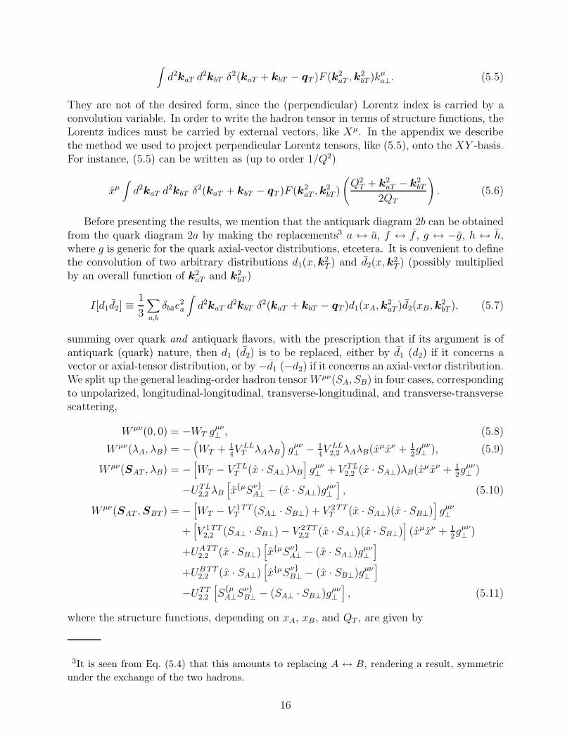
a⊥. (5.5)

They are not of the desired form, since the (perpendicular) Lorentz index is carried by aconvolution variable. In order to write the hadron tensor in terms of structure functions, theLorentz indices must be carried by external vectors, like Xµ. In the appendix we describethe method we used to project perpendicular Lorentz tensors, like (5.5), onto the XY -basis.For instance, (5.5) can be written as (up to order 1/Q2)

xµ∫

d2kaT d2kbT δ

2(kaT + kbT − qT )F (k2aT ,k

2bT )

(

Q2T + k2

aT − k2bT

2QT

)

. (5.6)

Before presenting the results, we mention that the antiquark diagram 2b can be obtainedfrom the quark diagram 2a by making the replacements3 a ↔ a, f ↔ f , g ↔ −g, h ↔ h,where g is generic for the quark axial-vector distributions, etcetera. It is convenient to definethe convolution of two arbitrary distributions d1(x,k

2T ) and d2(x,k

2T ) (possibly multiplied

by an overall function of k2aT and k2

bT )

I[d1d2] ≡1

3

∑

a,b

δbae2a

∫

d2kaT d2kbT δ

2(kaT + kbT − qT )d1(xA,k2aT )d2(xB,k

2bT ), (5.7)

summing over quark and antiquark flavors, with the prescription that if its argument is ofantiquark (quark) nature, then d1 (d2) is to be replaced, either by d1 (d2) if it concerns avector or axial-tensor distribution, or by −d1 (−d2) if it concerns an axial-vector distribution.We split up the general leading-order hadron tensorW µν(SA, SB) in four cases, correspondingto unpolarized, longitudinal-longitudinal, transverse-longitudinal, and transverse-transversescattering,

W µν(0, 0) = −WT gµν⊥ , (5.8)

W µν(λA, λB) = −(

WT + 14V LL

T λAλB

)

gµν⊥ − 1

4V LL

2,2 λAλB(xµxν + 12gµν⊥ ), (5.9)

W µν(SAT , λB) = −[

WT − V TLT (x · SA⊥)λB

]

gµν⊥ + V TL

2,2 (x · SA⊥)λB(xµxν + 12gµν⊥ )

−UTL2,2 λB

[

xµSνA⊥ − (x · SA⊥)gµν

⊥

]

, (5.10)

W µν(SAT ,SBT ) = −[

WT − V 1 TTT (SA⊥ · SB⊥) + V 2 TT

T (x · SA⊥)(x · SB⊥)]

gµν⊥

+[

V 1 TT2,2 (SA⊥ · SB⊥) − V 2 TT

2,2 (x · SA⊥)(x · SB⊥)]

(xµxν + 12gµν⊥ )

+UA TT2,2 (x · SB⊥)

[

xµSνA⊥ − (x · SA⊥)gµν

⊥

]

+UB TT2,2 (x · SA⊥)

[

xµSνB⊥ − (x · SB⊥)gµν

⊥

]

−UTT2,2

[

SµA⊥S

νB⊥ − (SA⊥ · SB⊥)gµν

⊥

]

, (5.11)

where the structure functions, depending on xA, xB, and QT , are given by

3It is seen from Eq. (5.4) that this amounts to replacing A ↔ B, rendering a result, symmetric

under the exchange of the two hadrons.

16

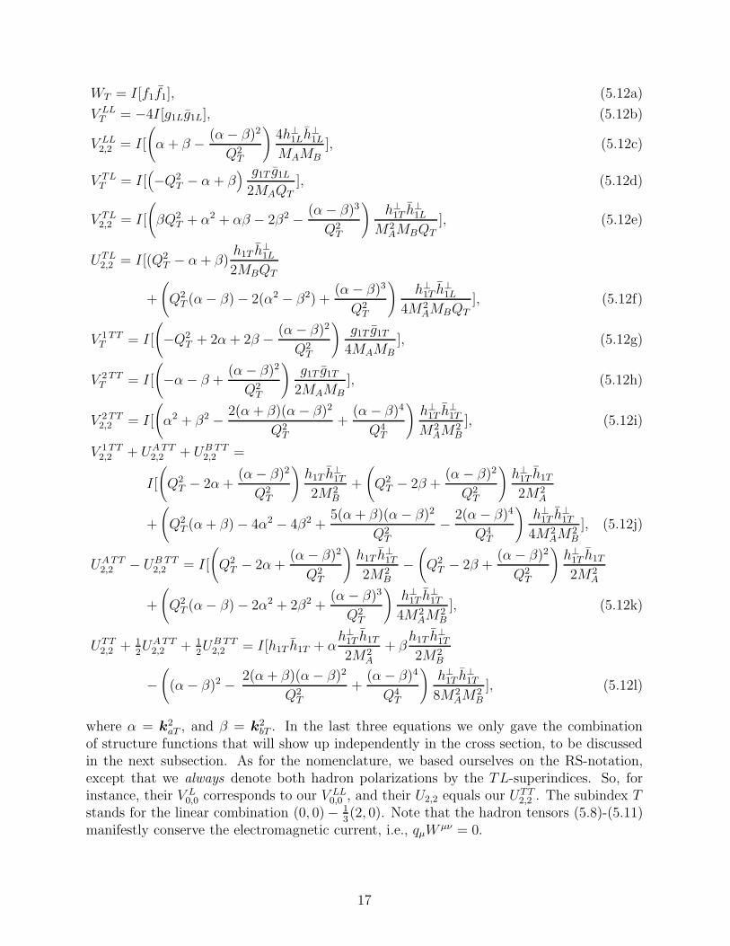
WT = I[f1f1], (5.12a)

V LLT = −4I[g1Lg1L], (5.12b)

V LL2,2 = I[

(

α + β − (α− β)2

Q2T

)

4h⊥1Lh⊥1L

MAMB

], (5.12c)

V TLT = I[

(

−Q2T − α + β

) g1T g1L

2MAQT], (5.12d)

V TL2,2 = I[

(

βQ2T + α2 + αβ − 2β2 − (α− β)3

Q2T

)

h⊥1T h⊥1L

M2AMBQT

], (5.12e)

UTL2,2 = I[(Q2

T − α + β)h1T h

⊥1L

2MBQT

+

(

Q2T (α− β) − 2(α2 − β2) +

(α− β)3

Q2T

)

h⊥1T h⊥1L

4M2AMBQT

], (5.12f)

V 1 TTT = I[

(

−Q2T + 2α + 2β − (α− β)2

Q2T

)

g1T g1T

4MAMB], (5.12g)

V 2 TTT = I[

(

−α − β +(α− β)2

Q2T

)

g1T g1T

2MAMB], (5.12h)

V 2 TT2,2 = I[

(

α2 + β2 − 2(α + β)(α− β)2

Q2T

+(α− β)4

Q4T

)

h⊥1T h⊥1T

M2AM

2B

], (5.12i)

V 1 TT2,2 + UA TT

2,2 + UB TT2,2 =

I[

(

Q2T − 2α+

(α− β)2

Q2T

)

h1T h⊥1T

2M2B

+

(

Q2T − 2β +

(α− β)2

Q2T

)

h⊥1T h1T

2M2A

+

(

Q2T (α+ β) − 4α2 − 4β2 +

5(α + β)(α− β)2

Q2T

− 2(α− β)4

Q4T

)

h⊥1T h⊥1T

4M2AM

2B

], (5.12j)

UA TT2,2 − UB TT

2,2 = I[

(

Q2T − 2α+

(α− β)2

Q2T

)

h1T h⊥1T

2M2B

−(

Q2T − 2β +

(α− β)2

Q2T

)

h⊥1T h1T

2M2A

+

(

Q2T (α− β) − 2α2 + 2β2 +

(α− β)3

Q2T

)

h⊥1T h⊥1T

4M2AM

2B

], (5.12k)

UTT2,2 + 1

2UA TT

2,2 + 12UB TT

2,2 = I[h1T h1T + αh⊥1T h1T

2M2A

+ βh1T h

⊥1T

2M2B

−(

(α− β)2 − 2(α+ β)(α− β)2

Q2T

+(α− β)4

Q4T

)

h⊥1T h⊥1T

8M2AM

2B

], (5.12l)

where α = k2aT , and β = k2

bT . In the last three equations we only gave the combinationof structure functions that will show up independently in the cross section, to be discussedin the next subsection. As for the nomenclature, we based ourselves on the RS-notation,except that we always denote both hadron polarizations by the TL-superindices. So, forinstance, their V L

0,0 corresponds to our V LL0,0 , and their U2,2 equals our UTT

2,2 . The subindex Tstands for the linear combination (0, 0)− 1

3(2, 0). Note that the hadron tensors (5.8)-(5.11)

manifestly conserve the electromagnetic current, i.e., qµWµν = 0.

17

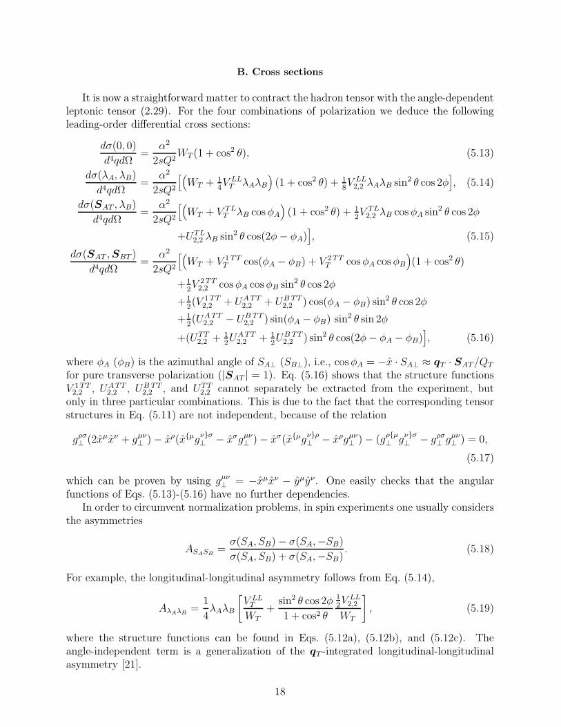
B. Cross sections

It is now a straightforward matter to contract the hadron tensor with the angle-dependentleptonic tensor (2.29). For the four combinations of polarization we deduce the followingleading-order differential cross sections:

dσ(0, 0)

d4qdΩ=

α2

2sQ2WT (1 + cos2 θ), (5.13)

dσ(λA, λB)

d4qdΩ=

α2

2sQ2

[(

WT + 14V LL

T λAλB

)

(1 + cos2 θ) + 18V LL

2,2 λAλB sin2 θ cos 2φ]

, (5.14)

dσ(SAT , λB)

d4qdΩ=

α2

2sQ2

[(

WT + V TLT λB cosφA

)

(1 + cos2 θ) + 12V TL

2,2 λB cosφA sin2 θ cos 2φ

+UTL2,2 λB sin2 θ cos(2φ− φA)

]

, (5.15)

dσ(SAT ,SBT )

d4qdΩ=

α2

2sQ2

[(

WT + V 1 TTT cos(φA − φB) + V 2 TT

T cosφA cosφB

)

(1 + cos2 θ)

+12V 2 TT

2,2 cosφA cosφB sin2 θ cos 2φ

+12(V 1 TT

2,2 + UA TT2,2 + UB TT

2,2 ) cos(φA − φB) sin2 θ cos 2φ

+12(UA TT

2,2 − UB TT2,2 ) sin(φA − φB) sin2 θ sin 2φ

+(UTT2,2 + 1

2UA TT

2,2 + 12UB TT

2,2 ) sin2 θ cos(2φ− φA − φB)]

, (5.16)

where φA (φB) is the azimuthal angle of SA⊥ (SB⊥), i.e., cosφA = −x · SA⊥ ≈ qT · SAT/QT

for pure transverse polarization (|SAT | = 1). Eq. (5.16) shows that the structure functionsV 1 TT

2,2 , UA TT2,2 , UB TT

2,2 , and UTT2,2 cannot separately be extracted from the experiment, but

only in three particular combinations. This is due to the fact that the corresponding tensorstructures in Eq. (5.11) are not independent, because of the relation

gρσ⊥ (2xµxν + gµν

⊥ ) − xρ(xµgνσ⊥ − xσgµν

⊥ ) − xσ(xµgνρ⊥ − xρgµν

⊥ ) − (gρµ⊥ g

νσ⊥ − gρσ

⊥ gµν⊥ ) = 0,

(5.17)

which can be proven by using gµν⊥ = −xµxν − yµyν. One easily checks that the angular

functions of Eqs. (5.13)-(5.16) have no further dependencies.In order to circumvent normalization problems, in spin experiments one usually considers

the asymmetries

ASASB=σ(SA, SB) − σ(SA,−SB)

σ(SA, SB) + σ(SA,−SB). (5.18)

For example, the longitudinal-longitudinal asymmetry follows from Eq. (5.14),

AλAλB=

1

4λAλB

[

V LLT

WT

+sin2 θ cos 2φ

1 + cos2 θ

12V LL

2,2

WT

]

, (5.19)

where the structure functions can be found in Eqs. (5.12a), (5.12b), and (5.12c). Theangle-independent term is a generalization of the qT -integrated longitudinal-longitudinalasymmetry [21].

18

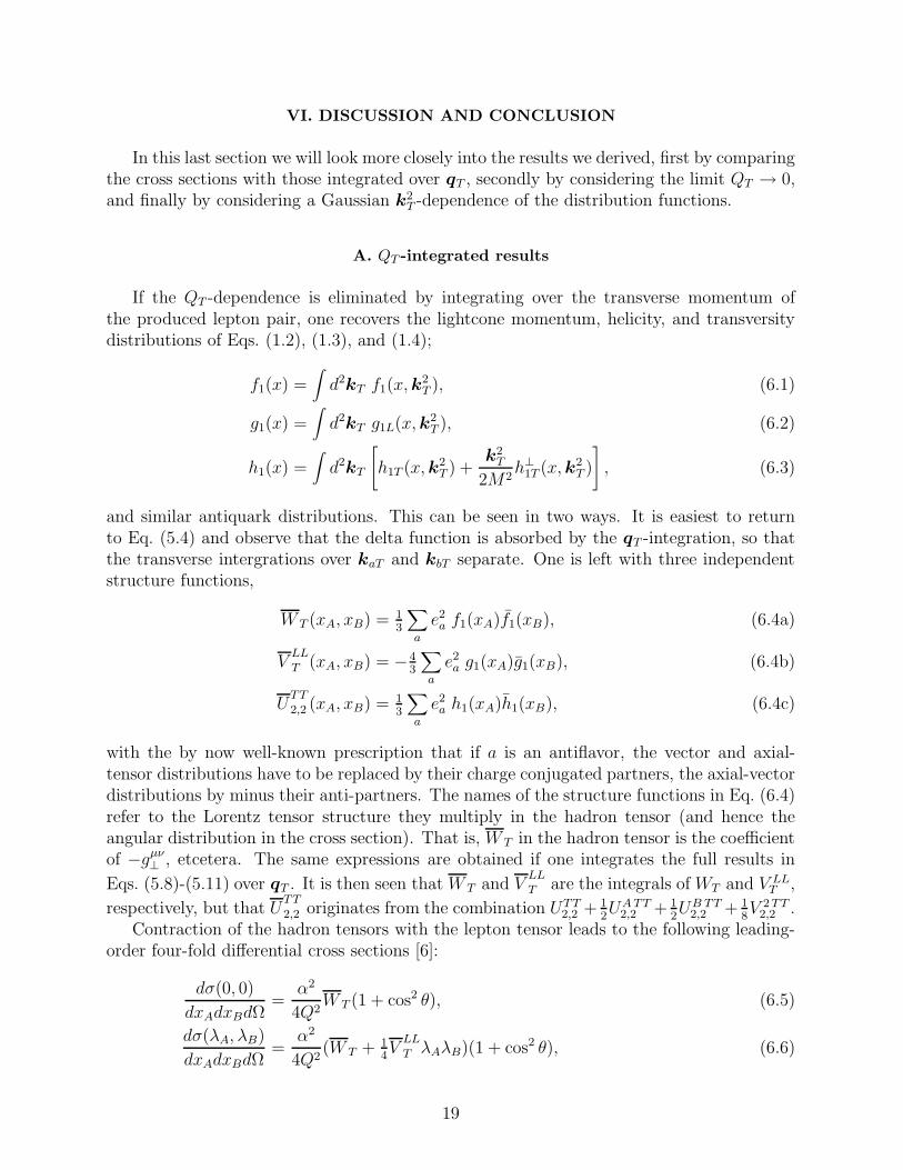
VI. DISCUSSION AND CONCLUSION

In this last section we will look more closely into the results we derived, first by comparingthe cross sections with those integrated over qT , secondly by considering the limit QT → 0,and finally by considering a Gaussian k2

T -dependence of the distribution functions.

A. QT -integrated results

If the QT -dependence is eliminated by integrating over the transverse momentum ofthe produced lepton pair, one recovers the lightcone momentum, helicity, and transversitydistributions of Eqs. (1.2), (1.3), and (1.4);

f1(x) =∫

d2kT f1(x,k2T ), (6.1)

g1(x) =∫

d2kT g1L(x,k2T ), (6.2)

h1(x) =∫

d2kT

[

h1T (x,k2T ) +

k2T

2M2h⊥1T (x,k2

T )

]

, (6.3)

and similar antiquark distributions. This can be seen in two ways. It is easiest to returnto Eq. (5.4) and observe that the delta function is absorbed by the qT -integration, so thatthe transverse intergrations over kaT and kbT separate. One is left with three independentstructure functions,

W T (xA, xB) = 13

∑

a

e2a f1(xA)f1(xB), (6.4a)

VLLT (xA, xB) = −4

3

∑

a

e2a g1(xA)g1(xB), (6.4b)

UTT2,2 (xA, xB) = 1

3

∑

a

e2a h1(xA)h1(xB), (6.4c)

with the by now well-known prescription that if a is an antiflavor, the vector and axial-tensor distributions have to be replaced by their charge conjugated partners, the axial-vectordistributions by minus their anti-partners. The names of the structure functions in Eq. (6.4)refer to the Lorentz tensor structure they multiply in the hadron tensor (and hence theangular distribution in the cross section). That is, W T in the hadron tensor is the coefficientof −gµν

⊥ , etcetera. The same expressions are obtained if one integrates the full results in

Eqs. (5.8)-(5.11) over qT . It is then seen that W T and VLLT are the integrals of WT and V LL

T ,

respectively, but that UTT2,2 originates from the combination UTT

2,2 + 12UA TT

2,2 + 12UB TT

2,2 + 18V 2 TT

2,2 .Contraction of the hadron tensors with the lepton tensor leads to the following leading-

order four-fold differential cross sections [6]:

dσ(0, 0)

dxAdxBdΩ=

α2

4Q2W T (1 + cos2 θ), (6.5)

dσ(λA, λB)

dxAdxBdΩ=

α2

4Q2(W T + 1

4V

LLT λAλB)(1 + cos2 θ), (6.6)

19

dσ(SAT , λB)

dxAdxBdΩ=

α2

4Q2W T (1 + cos2 θ), (6.7)

dσ(SAT ,SBT )

dxAdxBdΩ=

α2

4Q2

[

W T (1 + cos2 θ) + UTT2,2 sin2 θ cos(2φ− φA − φB)

]

. (6.8)

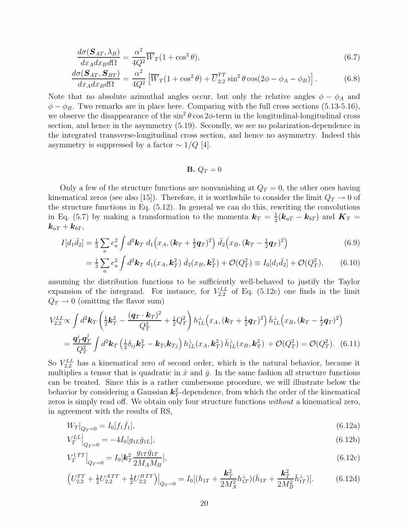
Note that no absolute azimuthal angles occur, but only the relative angles φ − φA andφ− φB. Two remarks are in place here. Comparing with the full cross sections (5.13-5.16),we observe the disappearance of the sin2 θ cos 2φ-term in the longitudinal-longitudinal crosssection, and hence in the asymmetry (5.19). Secondly, we see no polarization-dependence inthe integrated transverse-longitudinal cross section, and hence no asymmetry. Indeed thisasymmetry is suppressed by a factor ∼ 1/Q [4].

B. QT = 0

Only a few of the structure functions are nonvanishing at QT = 0, the other ones havingkinematical zeros (see also [15]). Therefore, it is worthwhile to consider the limit QT → 0 ofthe structure functions in Eq. (5.12). In general we can do this, rewriting the convolutionsin Eq. (5.7) by making a transformation to the momenta kT = 1

2(kaT − kbT ) and KT =

kaT + kbT ,

I[d1d2] = 13

∑

a

e2a

∫

d2kT d1

(

xA, (kT + 12qT )2

)

d2

(

xB, (kT − 12qT )2

)

(6.9)

= 13

∑

a

e2a

∫

d2kT d1(xA,k2T ) d2(xB,k

2T ) + O(Q2

T ) ≡ I0[d1d2] + O(Q2T ), (6.10)

assuming the distribution functions to be sufficiently well-behaved to justify the Taylorexpansion of the integrand. For instance, for V LL

2,2 of Eq. (5.12c) one finds in the limitQT → 0 (omitting the flavor sum)

V LL2,2 ∝

∫

d2kT

(

12k2

T − (qT · kT )2

Q2T

+ 12Q2

T

)

h⊥1L

(

xA, (kT + 12qT )2

)

h⊥1L

(

xB, (kT − 12qT )2

)

=qi

T qjT

Q2T

∫

d2kT

(

12δijk

2T − kT ikTj

)

h⊥1L(xA,k2T ) h⊥1L(xB,k

2T ) + O(Q2

T ) = O(Q2T ). (6.11)

So V LL2,2 has a kinematical zero of second order, which is the natural behavior, because it

multiplies a tensor that is quadratic in x and y. In the same fashion all structure functionscan be treated. Since this is a rather cumbersome procedure, we will illustrate below thebehavior by considering a Gaussian k2

T -dependence, from which the order of the kinematicalzeros is simply read off. We obtain only four structure functions without a kinematical zero,in agreement with the results of RS,

WT |QT =0 = I0[f1f1], (6.12a)

V LLT

∣

∣

∣

QT =0= −4I0[g1Lg1L], (6.12b)

V 1 TTT

∣

∣

∣

QT =0= I0[k

2T

g1T g1T

2MAMB], (6.12c)

(

UTT2,2 + 1

2UA TT

2,2 + 12UB TT

2,2

)∣

∣

∣

QT =0= I0[(h1T +

k2T

2M2A

h⊥1T )(h1T +k2

T

2M2B

h⊥1T )]. (6.12d)

20

An easier way to obtain this result is to start from Eq. (5.4), and put QT = 0 from there.One then never picks up the other structure functions in the first place. The cross sections atQT = 0 can be obtained by insertion of these structure functions into the explicit expressionsgiven for the cross sections in Eqs. (5.13)-(5.16).

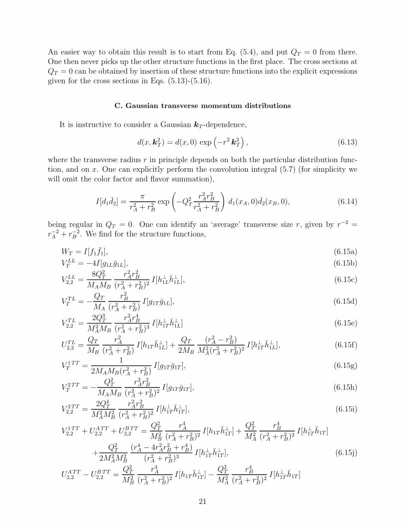
C. Gaussian transverse momentum distributions

It is instructive to consider a Gaussian kT -dependence,

d(x,k2T ) = d(x, 0) exp

(

−r2 k2T

)

, (6.13)

where the transverse radius r in principle depends on both the particular distribution func-tion, and on x. One can explicitly perform the convolution integral (5.7) (for simplicity wewill omit the color factor and flavor summation),

I[d1d2] =π

r2A + r2

B

exp

(

−Q2T

r2Ar

2B

r2A + r2

B

)

d1(xA, 0)d2(xB, 0), (6.14)

being regular in QT = 0. One can identify an ‘average’ transverse size r, given by r−2 =r−2A + r−2

B . We find for the structure functions,

WT = I[f1f1], (6.15a)

V LLT = −4I[g1Lg1L], (6.15b)

V LL2,2 =

8Q2T

MAMB

r2Ar

2B

(r2A + r2

B)2I[h⊥1Lh

⊥1L], (6.15c)

V TLT = −QT

MA

r2B

(r2A + r2

B)I[g1T g1L], (6.15d)

V TL2,2 =

2Q3T

M2AMB

r2Ar

4B

(r2A + r2

B)3I[h⊥1T h

⊥1L] (6.15e)

UTL2,2 =

QT

MB

r2A

(r2A + r2

B)I[h1T h

⊥1L] +

QT

2MB

(r2A − r2

B)

M2A(r2

A + r2B)2

I[h⊥1T h⊥1L], (6.15f)

V 1 TTT =

1

2MAMB(r2A + r2

B)I[g1T g1T ], (6.15g)

V 2 TTT = − Q2

T

MAMB

r2Ar

2B

(r2A + r2

B)2I[g1T g1T ], (6.15h)

V 2 TT2,2 =

2Q4T

M2AM

2B

r2Ar

2B

(r2A + r2

B)2I[h⊥1T h

⊥1T ], (6.15i)

V 1 TT2,2 + UA TT

2,2 + UB TT2,2 =

Q2T

M2B

r4A

(r2A + r2

B)2I[h1T h

⊥1T ] +

Q2T

M2A

r4B

(r2A + r2

B)2I[h⊥1T h1T ]

+Q2

T

2M2AM

2B

(r4A − 4r2

Ar2B + r4

B)

(r2A + r2

B)3I[h⊥1T h

⊥1T ], (6.15j)

UA TT2,2 − UB TT

2,2 =Q2

T

M2B

r4A

(r2A + r2

B)2I[h1T h

⊥1T ] − Q2

T

M2A

r4B

(r2A + r2

B)2I[h⊥1T h1T ]

21

+Q2

T

2M2AM

2B

(r2A − r2

B)

(r2A + r2

B)2I[h⊥1T h

⊥1T ], (6.15k)

UTT2,2 + 1

2UA TT

2,2 + 12UB TT

2,2 = I[h1T h1T ] +1

2M2A(r2

A + r2B)

(

1 +Q2T

r4B

r2A + r2

B

)

I[h⊥1T h1T ]

+1

2M2B(r2

A + r2B)

(

1 +Q2T

r4A

r2A + r2

B

)

I[h1T h⊥1T ]

+1

2M2AM

2B(r2

A + r2B)2

(

1 +Q2

T

2

(r2A − r2

B)2

r2A + r2

B

)

I[h⊥1T h⊥1T ]. (6.15l)

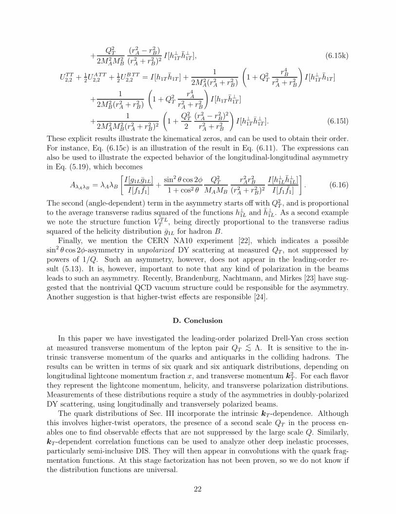
These explicit results illustrate the kinematical zeros, and can be used to obtain their order.For instance, Eq. (6.15c) is an illustration of the result in Eq. (6.11). The expressions canalso be used to illustrate the expected behavior of the longitudinal-longitudinal asymmetryin Eq. (5.19), which becomes

AλAλB= λAλB

[

I[g1Lg1L]

I[f1f1]+

sin2 θ cos 2φ

1 + cos2 θ

Q2T

MAMB

r2Ar

2B

(r2A + r2

B)2

I[h⊥1Lh⊥1L]

I[f1f1]

]

. (6.16)

The second (angle-dependent) term in the asymmetry starts off with Q2T , and is proportional

to the average transverse radius squared of the functions h⊥1L and h⊥1L. As a second examplewe note the structure function V TL

T , being directly proportional to the transverse radiussquared of the helicity distribution g1L for hadron B.

Finally, we mention the CERN NA10 experiment [22], which indicates a possiblesin2 θ cos 2φ-asymmetry in unpolarized DY scattering at measured QT , not suppressed bypowers of 1/Q. Such an asymmetry, however, does not appear in the leading-order re-sult (5.13). It is, however, important to note that any kind of polarization in the beamsleads to such an asymmetry. Recently, Brandenburg, Nachtmann, and Mirkes [23] have sug-gested that the nontrivial QCD vacuum structure could be responsible for the asymmetry.Another suggestion is that higher-twist effects are responsible [24].

D. Conclusion

In this paper we have investigated the leading-order polarized Drell-Yan cross sectionat measured transverse momentum of the lepton pair QT

<∼ Λ. It is sensitive to the in-trinsic transverse momentum of the quarks and antiquarks in the colliding hadrons. Theresults can be written in terms of six quark and six antiquark distributions, depending onlongitudinal lightcone momentum fraction x, and transverse momentum k2

T . For each flavorthey represent the lightcone momentum, helicity, and transverse polarization distributions.Measurements of these distributions require a study of the asymmetries in doubly-polarizedDY scattering, using longitudinally and transversely polarized beams.

The quark distributions of Sec. III incorporate the intrinsic kT -dependence. Althoughthis involves higher-twist operators, the presence of a second scale QT in the process en-ables one to find observable effects that are not suppressed by the large scale Q. Similarly,kT -dependent correlation functions can be used to analyze other deep inelastic processes,particularly semi-inclusive DIS. They will then appear in convolutions with the quark frag-mentation functions. At this stage factorization has not been proven, so we do not know ifthe distribution functions are universal.

22

ACKNOWLEDGMENTS

We acknowledge numerous discussions with J. Levelt (Erlangen). This work was sup-ported by the Foundation for Fundamental Research on Matter (FOM) and the NationalOrganization for Scientific Research (NWO).

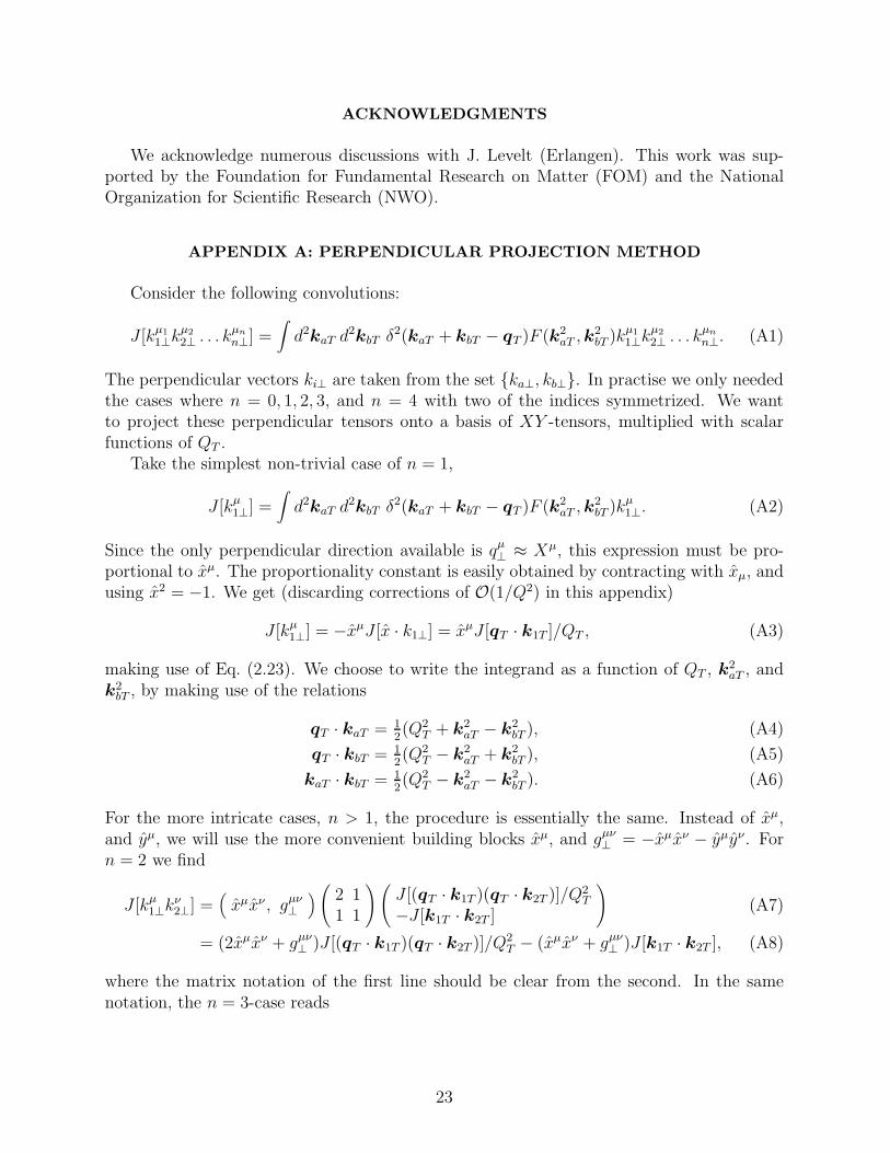
APPENDIX A: PERPENDICULAR PROJECTION METHOD

Consider the following convolutions:

J [kµ1

1⊥kµ2

2⊥ . . . kµn

n⊥] =∫

d2kaT d2kbT δ

2(kaT + kbT − qT )F (k2aT ,k

2bT )kµ1

1⊥kµ2

2⊥ . . . kµn

n⊥. (A1)

The perpendicular vectors ki⊥ are taken from the set ka⊥, kb⊥. In practise we only neededthe cases where n = 0, 1, 2, 3, and n = 4 with two of the indices symmetrized. We wantto project these perpendicular tensors onto a basis of XY -tensors, multiplied with scalarfunctions of QT .

Take the simplest non-trivial case of n = 1,

J [kµ1⊥] =

∫

d2kaT d2kbT δ

2(kaT + kbT − qT )F (k2aT ,k

2bT )kµ

1⊥. (A2)

Since the only perpendicular direction available is qµ⊥ ≈ Xµ, this expression must be pro-

portional to xµ. The proportionality constant is easily obtained by contracting with xµ, andusing x2 = −1. We get (discarding corrections of O(1/Q2) in this appendix)

J [kµ1⊥] = −xµJ [x · k1⊥] = xµJ [qT · k1T ]/QT , (A3)

making use of Eq. (2.23). We choose to write the integrand as a function of QT , k2aT , and

k2bT , by making use of the relations

qT · kaT = 12(Q2

T + k2aT − k2

bT ), (A4)

qT · kbT = 12(Q2

T − k2aT + k2

bT ), (A5)

kaT · kbT = 12(Q2

T − k2aT − k2

bT ). (A6)

For the more intricate cases, n > 1, the procedure is essentially the same. Instead of xµ,and yµ, we will use the more convenient building blocks xµ, and gµν

⊥ = −xµxν − yµyν. Forn = 2 we find

J [kµ1⊥k

ν2⊥] =

(

xµxν , gµν⊥

)

(

2 11 1

)(

J [(qT · k1T )(qT · k2T )]/Q2T

−J [k1T · k2T ]

)

(A7)

= (2xµxν + gµν⊥ )J [(qT · k1T )(qT · k2T )]/Q2

T − (xµxν + gµν⊥ )J [k1T · k2T ], (A8)

where the matrix notation of the first line should be clear from the second. In the samenotation, the n = 3-case reads

23

J [kµ1⊥k

ν2⊥k

ρ3⊥] =

(

xµxν xρ, xρgµν⊥ , xνgµρ

⊥ , xµgνρ

⊥

)

×

4 1 1 11 1 0 01 0 1 01 0 0 1

J [(qT · k1T )(qT · k2T )(qT · k3T )]/Q3T

−J [(qT · k3T )(k1T · k2T )]/QT

−J [(qT · k2T )(k1T · k3T )]/QT

−J [(qT · k1T )(k2T · k3T )]/QT

. (A9)

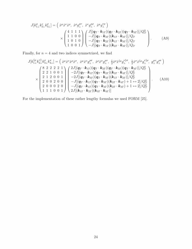
Finally, for n = 4 and two indices symmetrized, we find

J [kµ1⊥k

ν2⊥k

ρ3⊥k

σ4⊥] =

(

xµxν xρxσ, xµxνgρσ⊥ , x

ρxσgµν⊥ , 1

2xρxµg

νσ⊥ , 1

2xσxµg

νρ⊥ , gµν

⊥ gρσ⊥

)

×

8 2 2 2 2 12 2 1 0 0 12 1 2 0 0 12 0 0 2 0 02 0 0 0 2 01 1 1 0 0 1

2J [(qT · k1T )(qT · k2T )(qT · k3T )(qT · k4T )]/Q4T

−2J [(qT · k1T )(qT · k2T )(k3T · k4T )]/Q2T

−2J [(qT · k3T )(qT · k4T )(k1T · k2T )]/Q2T

−J [(qT · k1T )(qT · k3T )(k2T · k4T ) + 1 ↔ 2]/Q2T

−J [(qT · k1T )(qT · k4T )(k2T · k3T ) + 1 ↔ 2]/Q2T

2J [(k1T · k2T )(k3T · k4T )]

. (A10)

For the implementation of these rather lengthy formulas we used FORM [25].

24

REFERENCES

[1] J. Ashman et al., Phys. Lett. B 206, 364 (1988); B. Adeva et al., ibid. 302, 533 (1993).[2] D. E. Soper, Phys. Rev. D 15, 1141 (1977); Phys. Rev. Lett. 43, 1847 (1979).[3] R. L. Jaffe, Nucl. Phys. B 229, 205 (1983).[4] R. L. Jaffe and X. Ji, Phys. Rev. Lett. 67, 552 (1991); Nucl. Phys. B 375, 527 (1992).[5] J. L. Cortes, B. Pire, and J. P. Ralston, Z. Phys. C 55, 409 (1992).[6] J. P. Ralston and D. E. Soper, Nucl. Phys. B 152, 109 (1979).[7] X. Artru and M. Mekhfi, Z. Phys. C 45, 669 (1990).[8] X. Ji, Phys. Lett. B 284, 137 (1992).[9] J. Levelt and P. J. Mulders, Phys. Rev. D 49, 96 (1994).

[10] S. D. Drell and T.-M. Yan, Phys. Rev. Lett. 25, 316 (1970); Ann. Phys. (N.Y.) 66, 578(1971).

[11] J. C. Collins, D. E. Soper, and G. Sterman, Nucl. Phys. B 250, 199 (1985).[12] J. C. Collins, Nucl. Phys. B 394, 169 (1993).[13] J. C. Collins, D. E. Soper, and G. Sterman, in Pertubative Quantum Chromomdynamics,

edited by A. H. Mueller (World Scientific, Singapore, 1989).[14] R. K. Ellis, W. Furmanski, and R. Petronzio, Nucl. Phys. B 207, 1 (1982); 212, 29

(1983).[15] C. S. Lam and W.-K. Tung, Phys. Rev. D 7, 2447 (1978).[16] J. T. Donohue and S. Gottlieb, Phys. Rev. D 23, 2577, 2581 (1981).[17] J. C. Collins and D. E. Soper, Phys. Rev. D 16, 2219 (1977).[18] R. D. Tangerman and P. J. Mulders, in preparation.[19] J. B. Kogut and D. E. Soper, Phys. Rev. D 1, 2901 (1970).[20] C. Itzykson and J.-B. Zuber, Quantum Field Theory (McGraw-Hill, New York, 1985).[21] F. E. Close and D. Sivers, Phys. Rev. Lett. 39, 1116 (1977).[22] S. Falciano et al., Z. Phys. C 31, 513 (1986); M. Guanziroli et al., ibid. 37, 545 (1988).[23] A. Brandenburg, O. Nachtmann, and E. Mirkes, Z. Phys. C 60, 697 (1993).[24] A. Brandenburg, S. J. Brodsky, V. V. Khoze, and D. Muller, preprint SLAC-PUB-6464,

hep-ph/9403361.[25] J. A. M. Vermaseren, Symbolic manipulation with FORM, version 2 (CAN, Kruislaan

413, 1098 SJ Amsterdam, 1991).

25

FIGURES

FIG. 1. Quark and antiquark handbag diagrams for inclusive DIS.

FIG. 2. The quark and antiquark Born diagrams for the Drell-Yan process.

FIG. 3. The blob representing the quark correlation function.

26

This figure "fig1-1.png" is available in "png" format from:

http://arxiv.org/ps/hep-ph/9403227