Embed Size (px)
Citation preview
/Z.
x ih~FfECP
NLCT
4QF
.489
4 / ____Now
AFIT/GE/ENG/88D-19
AJ
FLIGHT CONTROLLER DESIGN WITHNONLINEAR AERODYNAMICS, LARGE
PARAMETER UNCERTAINTY, AND PILOTCOMPENSATION
THESISThomas John KobylarzFirst Lieutenant, USAF
AFIT/GE/ENG/88D-19
L-DTc~E" ETE
7 JAN 1989 1
Approved for public release; distribution unlimited
AFIT/GE/ENG/88D-19
FLIGHT CONTROLLER DESIGN WITH NONLINEAR
AERODYNAMICS, LARGE PARAMETER UNCERTAINTY,
AND PILOT COMPENSATION
THESIS
Presented to the Faculty of the School of Engineering
of the Air Force Institute of Technology
j Air University
In Partial Fulfillment of the
Requirements for the Degree ofi Accession For
Master of Science in Electrical Engineering AT-esIS GIF-
DTIC TABUnannounced QJustification
Thomas John Kobylarz, B.S.E.E.
First Lieutenant, USAF Distribution/Availability Codes
Avai-andi/Or1st Special
December, 1988
Approved for public release; distribution unlimited
Acknowledgments
I would like to thank all my instructors P+ AFIT for providing me with the
foundation for completing this research, especially my thesis committee, Dr. Con-
stantine Houpis, Dr. Issac Horowitz and Lt Col Zdzislaw Lewantowicz. Without
them this thesis would have never been completed. The weekend discussions with
Dr. Horowitz were invaluable for the insight into the problem they provided to
both of us, thdnks afain. Thanks to Finley Barfield whose guidance kept these
results in line with reality.
Never ending thanks goes out to my beautiful wife4I for forcing me
to sit down and complete this work, as well as providing me with a list of home
improvements to breakup the monotony of such a large task. Of course a can't
leave out the kids; thnnkss ndw and to all the guys on the
Hockey, Football, and Softball teams, thanks for letting me bang my head a little.
To my classmates Captains Kurt Neumann and Daryl Hammond a special
thanks goes out for the enlightening conversioais at the annex. To Ron L, Larry,
Dave, Brian, Steve, and Chuck, what's life without a little fun.
Finally, I would like to dedicate this work to my loving mothei for 25
years of inspiration.
Thomas John Kobylarz
ii
Table of Contents
Page
Acknowledgments......................................ii
Tabie of Contents......................................iii
List of Figures .. .. .. .. ... ... ... ... ... ... ... ....... vii
List of Tables. .. .. ... ... ... ... ... .. ... ... ... .... xi
Abstract .. .. .. ... ... ... ... ... ... ... .. ... ...... xii
I. Background........ .. .. .. .. .. .. .. .. .. .. .. . . ....
Introduction.... .. .. .. .. .. .. .. .. .. .. .. . ....
Problem Statement .. .. .. .. ... ... ... ... ..... 1-2
Review of Current Literature. .. .. .. .. .. ... ...... 1-2
Current Approach .. .. .. .. .. .. ... ... ..... 1-2
Current Techniques. .. .. .. .. .. ... ... ..... 1-3
Uncertain vs. Deterministic Models. .. .. .. .. .... 1-3
The Quantitative Approach. .. .. .. .. ... ..... 1-4
Linear Time-Invariant QFT. .. .. .. .. ... ..... 1-5
Non-Linear QFT. .. .. .. .. ... ... ... ..... 1-6
Summary .. .. .. .. .. .. .. ... ... ... ..... 1-6
Assumptions. .. .. .. .. ... ... ... ... .. ...... 1-7
Scope .. .. .. .. .. ... ... ... ... ... ... ..... 1-8
Approach. .. .. .. .. .. ... ... ... ... ... ..... 1-8
Presentation. .. .. .. .. ... ... ... ... ... ..... 1-9
iii
Page
*II. Nonlinear QFT Theory. .. .. .. ... ... ... ... ... ... 2-1
Introduction. .. .. .. .. ... ... ... ... ... ..... 2-1
Linear SISO Case. .. .. .. .. ... ... ... ... ..... 2-1
Nonlinear SISO Case .. .. .. .. ... ... ... ... ... 2-2
Direct Analytical Model. .. .. .. .. ... .. ..... 2-2
Non-Direct Analytical Model .. .. .. .. .. .. ..... 2-4
Summary. .. .. .. .. .. ... ... ... ... ... ..... 2-4
III. Derivation of the LTI Equivalent Plants. .. .. .. ... ... ... 3-1
Introduction. .. .. .. .. ... ... ... ... ... ..... 3-1
The Simulator. .. .. .. .. ... ... ... ... ... ... 3-1
The Equivalent Plants. .. .. .. ... ... ... ... ... 3-2
Summary. .. .. .. .. .. ... ... ... ... ... ..... 3-5
(.IV. Design of the Inner Loop Controller .. .. .. ... .. ... ..... 4-1
Introduction. .. .. .. .. ... ... ... ... ... ..... 4-1
Bounds on L,(s) .. .. .. .. .. ... ... ... ... ..... 4-1
Modified Tracking Bounds .. .. .. .. .. ... ..... 4-2
Stability Bounds ... .. .. .. .. .. ... ... ..... 4-6
The Shaping of L,(s) .. .. .. .. ... ... ... ... ... 4-6
Interpretation of the Boundaries. .. .. .. .. .. .... 4-8
Proposed G(s) .. .. .. .. .. .. ... ... ... ... 4-9
Final Design of G(s). .. .. .. .. ... ... ...... 4-11
The Design of the Prefilter F(s). .. .. .. .. .. ... 4-12
Summary .. .. .. .. .. ... ... ... ... ... .. ... 4-15
V. Simulation of the Inner Loop SAS .. .. .. ... ... ... ..... 5-1
Introduction. .. .. .. .. ... ... ... ... ... ..... 5-1
MATRIEX Linear Simulation .. .. .. ... ... ... ... 5-1
iv
Page
Nonlinear Simulation .. .. .. .. ... ... ... ... ... 5-2
Nominal Flight Condition Simulation .. .. .. .. .... 5-3
Expanding the Envelope. .. .. .. .. .. ... ..... 5-5
Equivalent Inner Loop .. .. .. ... ... ... .. ...... 5-9
Summary .. .. .. .. .. ... ... ... ... ... ...... 5-10
VI. Pilot Compensation .. .. .. ... .. ... ... ... ... ..... 6-i
Introduction. .. .. .. .. ... ... ... ... ... ..... 6-1
The Pilot Model .. .. .. .. .. ... ... ... ... ..... 6-1
Transforming Analysis to Synthesis .. .. .. .. ... ..... 6-2
Synthesis of the Pilot Compensation Fp(.s) .. .. .. ....... &3
Pilot's View of Good Tracking Performance. .. ..... 6-3
Shaping the Response. .. .. .. .. .. .. ... ..... 6-6
Simulation of the Pilot Compensation. .. .. .. .. ...... 6-10
Summary .. .. .. .. .. ... ... ... ... ... ...... 6-13
VII. Conclusions and Recommuendations. .. .. ... ... ... ..... 7-1
Discussion .. .. .. .. ... ... ... ... ... ... .... 7-1
Conclusions. .. .. .. ... ... ... ... ... ... .... 7-2
Recommendations. .. .. .. .. ... ... ... ... ..... 7-3
Summary. .. .. .. .. .. ... ... ... ... ... ..... 7-4
A. Equivalent LTI Plants .. .. .. .. ... ... ... ... ... ... A-1
C* Transfer Functions for Ig Responses .. .. .. .. .. .... A-i
C' Transfer Functions for 2g Responses .. .. .. .. .. .... A-2
Validation of the LTI Transfer Functions .. .. .. .. ..... A-3
B. Boundary Data. .. .. ... ... ... ... ... ... ... .... B-i
Frequency Domain Tracking Bounds: .. .. .. .. ... .... B-i
Plant Templates .. .. .. .. .. ... ... ... ... ..... B-3
v
Page
C. Simulation of the Stability Augmentation System ............ C-1
Generation of the Nonlinear Prefilter ................ C-1
Results of Expanding the Envelope ................. C-2
D. Fourth Order Pad4 Approximation ...................... D-1
The General Padi Method ........................ D-1
The Approximation ............................ D-2
Bibliography ....... ................................. BIB-i
Vita ........ ..................................... VITA-i
vi
List of Figures
Figure Page
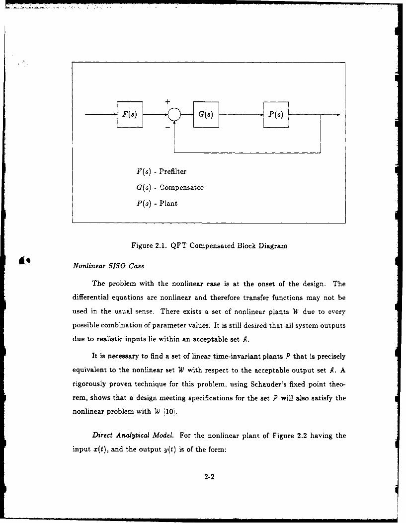
2.1. QFT Compensated Block Diagram ...... ................. 2-2
2.2. Nonlinear Plant Set ........ ......................... 2-3
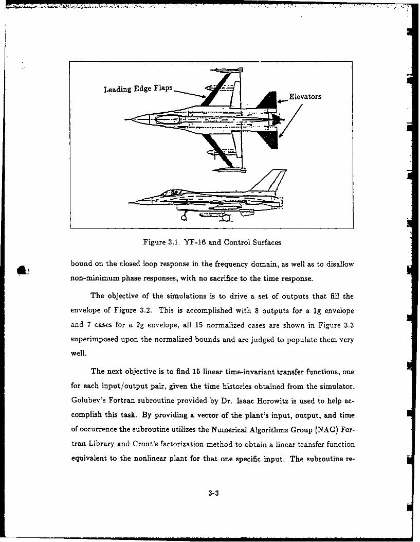
3.1. YF-16 and Control Surfaces ........ .................... 3-3
3.2. Normalized Bounds on the Output C" ...... .............. 3-4
3.3. Simulator Outputs used to Generate Plants ................. 3-4
3.4. Response of YF-16 and Equivalent Plant to the Same Input 3-6
4.1. Closed Loop Tracking Bounds in the Frequency Domain . 4-2
4.2. Example of Modified Tracking Bounds at w = 1 rad/sec ..... 4-3
4.3. Calculation of Bounds on F(jl) for the ABCD Template . . .. 4-4
(. 4.4. Bounds B(w) on Lo(jw) and Response of Proposed Design . . . 4-7
4.5. Response of Plant # 15 for Initial Design ..... ............. 4-10
4.6. Closed Loop Frequency Response of Plant # 15 .... ......... 4-10
4.7. Frequency Response of G(s) ...... .................... 4-13
4.8. Nominal Loop Transmission L,(j.) Designed ............... 4-13
4.9. Desired and Actual Variation in Closed Loop Response without
F(s)....... .................................. 4-14
4.10. Bounds on Prefilter and Proposed F(jw) ................. 4-14
5.1. MATRIXX Simulation of SAS Over Range of Uncertainty . . .. 5-2
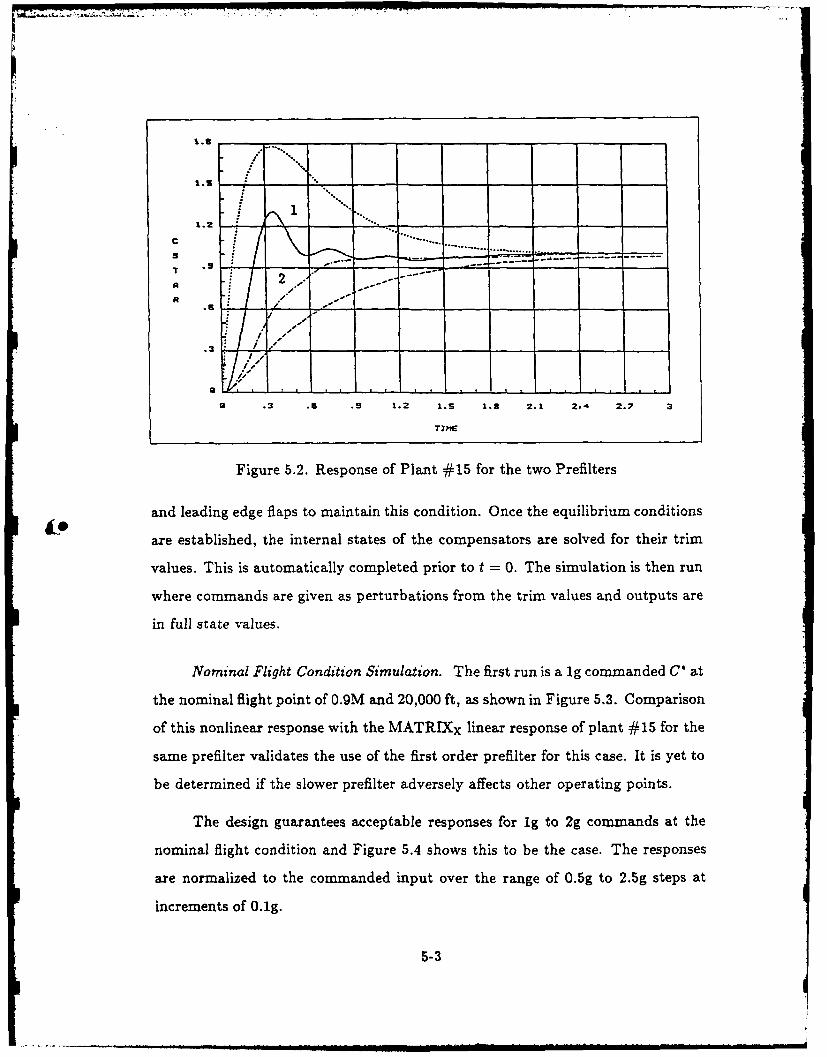
5.2. Response of Plant #15 for the two Prefilters ..... ........... 5-3
5.3. Response for 1g Command of Plant #15 and Nonlinear Aircraft 5-4
5.4. Normalized C' Response at Nominal Flight Condition ...... .... 5-4
5.5. Normalized C' Responses for 1-gg Commands at Nominal. . .. 5-6
5.6. Surface Deflections and Rates for 9g Command at Nominal . . . 5-7
vii
_ _ 5 U I- El U H_ II I . _i im I! i. iL . . .~i . -11 -.1 I , . . .. .
Figure Page
5.7. Aircraft Response to 9g Command at Nominal .............. 5-8
5.8. Flight Envelope of Acceptable SAS Responses .............. 5-9
5.9. Outputs of P,(s) and YF-16 for Step Input ................ 5-10
6.1. Form of Pilot Compensation ...... .................... 6-2
6.2. Nichols Chart Representation of Standards of Performance . . . 6-5
6.3. Starting Point for the Design of Fr(s) ..... ............... 6-7
6.4. Response Showing Cause of High Frequency Resonance ..... 6-8
6.5. Response and Standards of Performance for Final Design . ... 6-9
6.6. Closed Loop Frequency Response ..... ................. 6-10
6.7. Effect of Using Pad4 Approximation .................... 6-11
6.8. Nonlinear Response to C,,d = Ig. ...................... 6-12
6.9. Simulations for Trimmed Load Factors of 1g to 5gs .......... 6-13
A.I. Outputs of LTI Plant #1 and of YF-16 for the Same Input . . A-3
A.2. Outputs of LTI Plant #2 and of YF-16 for the Same Input . . . A-4
A.3. Outputs of LTI Plant #3 and of YF-16 for the Same Input . . . A-4
A.4. Outputs of LTI Plant #4 and of YF-16 for the Same Input . . . A-5
A.5. Outputs of LTI Plant #5 and of YF-16 for the Same Input . . . A-5
A.6. Outputs of LTI Plant #6 and of YF-16 for the Same Input . . . A-6
A.7. Outputs of LTI Plant #7 and of YF-16 for the Same Input . . . A-6
A.8. Outputs of LTI Plant #8 and of YF-16 for the Same Input . . . A-7
A.9. Outputs of LTI Plant #9 and of YF-16 for the Same Input . . . A-7
A.10.Outputs of LTI Plant #10 and of YF-16 for the Same Input A-8
A.11.Outputs of LTI Plant #11 and of YF-16 for the Same Input A-8
A.12.Outputs of LTI Plant #12 and of YF-16 for the Same Input A-9
A.13.Outputs of LTI Plant #13 and of YF-16 for the Same Input A-9
A.14.Outputs of LTI Plant #14 and of YF-16 for the Same Input A-10
viii
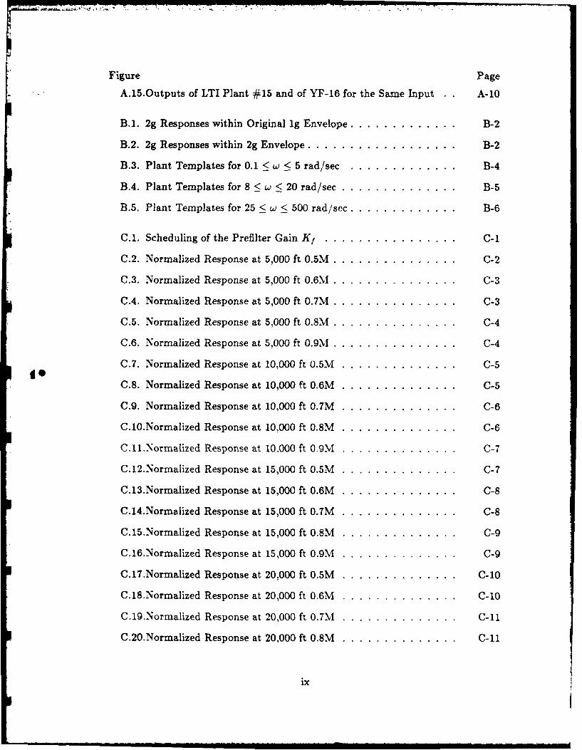
Figure Page
A.15.Outputs of LTI Plant #15 and of YF-16 for the Same Input .. A-10
B.1. 2g Responses within Original ig Envelope. .. .. .. .. .. ..... B-2
B.2. 2g Responses within 2g Envelope. .. .. .. .. ... .. ... ... B-2
B.3. Plant Templates for 0.1 < w < 5 rad/sec .. .. .. ... ... ... B-4
B.4. Plant Templates for 8 < w < 20 rad/sec .. .. .. .. .. ... .... B-5
B.5. Plant Templates for 25 < w < 500 rad/se . .. .. .. .. .. ..... B-6
0.1. Scheduling of the Prefilter Gain K1 . . . . . . . . . . . . . . . .. . . C-1
0.2. Normalized Response at 5,000 ft 0.5M .. .. .. .. .... .......- 2
0.3. Normalized Response at 5,000 ft O.6M1.. .. .. ... ... ...... C-3
C.4. Normalized Response at 5,000 ft 0.7M .. .. .. ... ... ...... C-3
C.5. Normalized Response at 5,000 ft 0.8M . . .. .. .. .. .. . . 0-4
0.6 Normalized Response at 5,000 ft 0.9M .. .. .. ... ... ...... C-4
C.7. Normalized Response at 10,000 ft 0.5M. .. .. ... ... .......- 5
0.8. Normalized Response at 10,000 ft 0.6M. .. .. .. ... .. ......- 5
0.9. Normalized Response at 10,000 ft 0.7M. .. .. ... ... .......- 6
C.10.Normalized Response at 10,000 ft 0.8M. .. .. ... ... .......- 6
C.11.N-ormalized Response at 10,000 ft 0.9M . .. .. ... ... .......- 7
C-12.Normalized Response at 15,000 ft 0.5M. .. .. ... ... .......- 7
C.13.Normalized Response at 15,000 ft 0.6M. .. .. ... ... .......- 8
C.14.Normalized Response at 15,000 ft 0.7M. .. .. ... ... .......- 8
C.15.Normalized Response at 15,000 ft 0.8M . .. .. ... ..........- 9
C.16.Normalized Response at 15,000 ft 0.9M. .. .. ... ... .......- 9
C.17.Normalized Response at 20,000 ft 0.5M .. .. .. ... .... ....- 10
C.18.Normalized Response at 20,000 ft 0.6M .. .. .. .... ... ....- 10
C.19.Normalized Response at 20,000 ft 0.7M .. .. .. .... ... ... C-11
0.20.Normalized Response at 20,000 ft 0.8M .. .. .. .... ... ... C-i1
ix
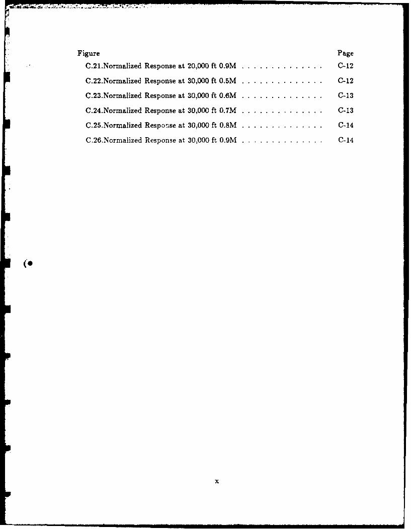
Figure Page
C.21.Normalized Response at 20,000 ft O.OM .. .. .. .. ... .......- 12
C.22.Normalized Response at 30,000 ft 0.5M .. .. .. .. ... .......- 12
C.23.Normalized Response at 30,000 ft 0.6M .. .. .. .. ... .......- 13
C.24.Normalized Response at 30,000 ft 0.7M .. .. .. .. ... ...... C-13
C.25.Norxnalized Respon~se at 30,000 ft 0.8M .. .. .. .. ... .......- 14
C.26.Norxnalized Response at 30,000 ft 0.9M .. .. .. .. ... .......- 14
x
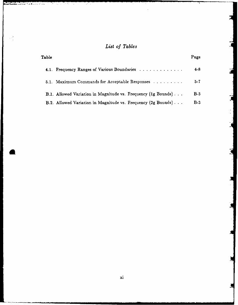
List of Tables
Table Page
4.1. Frequency Ranges of Various Boundaries ..... ............. 4-8
5.1. Maximum Commands for Acceptable Responses ............. 5-7
B.1. Allowed Variation in Magnitude vs. Frequency (ig Bounds) . . B-3
B.2. Allowed Variation in Magnitude vs. Frequency (2g Bounds) . . B-3
xi
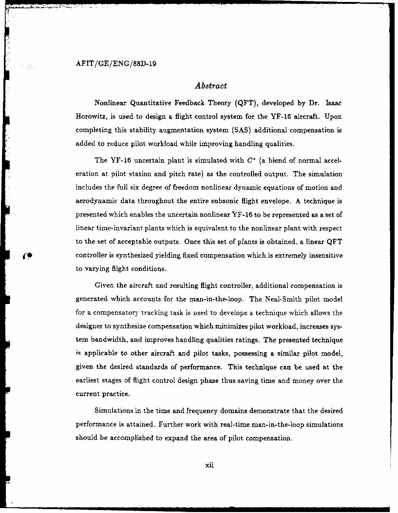
AFIT/GE/ENG/SSD-i9
Abstract
Nonlinear Quantitative Feedback Theory (QFT), developed by Dr. Isaac
Horowitz, is used to design a flight control system for the YF-16 aircraft. Upon
completing this stability augmentation system (SAS) additional compensation is
added to reduce pilot workload while improving handling qualities.
The YF-16 uncertain plant is simulated with C' (a blend of normal accel-
eration at pilot station and pitch rate) as the controlled output. The simulation
includes the full six degree of freedom nonlinear dynamic equations of motion and
aerodynamic data throughout the entire subsonic flight envelope. A technique is
presented which enables the uncertain nonlinear YF-16 to be represented as a set of
linear time-invariant plants which is equivalent to the nonlinear plant with respect
to the set of acceptable outputs. Once this set of plants is obtained, a linear QFT
controller is synthesized yielding fixed compensation which is extremely insensitive
to varying flight conditions.
Given the aircraft and resulting flight controller, additional compensation is
generated which accounts for the man-in-the-loop. The Neal-Smith pilot model
for a compensatory tracking task is used to develope a technique which allows the
designer to synthesize compensation which minimizes pilot workload, increases sys-
tem bandwidth, and improves handling qualities ratings. The presented technique
is applicable to other aircraft and pilot tasks, possessing a similar pilot model,
given the desired standards of performance. This technique can be used at the
earliest stages of flight control design phase thus saving time and money over the
current practice.
Simulations in the time and frequency domains demonstrate that the desired
performance is attained. Further work with real-time man-in-the-loop simulations
should be accomplished to expand the area of pilot compensation.
xii
"*-'t"a . . . . . . . . . . . . . ... ...- . .M ..... S...
FLIGHT CONTROLLER DESIGN WITH NONLINEAR
AERODYNAMICS, LARGE PARAMETER UNCERTAINTY,
AND PILOT COMPENSATION
L Background
Introduction
The design of a flight control system which allows the pilot to maneuver an
aircraft to desired flight paths is a major task. The maneuverability and speeds
required of modern aircraft place forces on the airframe that are too large for the
pilot to control. Also, the dynamic responses of the basic airframe are usually
unsatisfactory, even to the point of being so unstable that the aircraft is totally
uncontrollable by the pilot alone. The flight controller aids the pilot in performing
the tasks which allow him to accomplish the mission.
In order to design the controller, extensive modeling of the aircraft dynamics
is required. including the aerodynamic forces. The parameters in these models vary
drastically from one flight condition to another and are not precisely known for any
given flight condition. Research has shown that the flight controller design must be
sufficiently robust to handle these parameter variations if the desired performance
is to be obtained over a variety of flight conditions [19].
For certain missions the models of the aircraft system are also highly nonlin-
ear, with uncertain model parameters which challenges the engineer because the
mathematical analysis tools available are limited. Nonlinear quantitative feedback
theory allows the controls engineer to take both of these aspects into account at
the onset of the design and guarantees that the design will be acceptable for the
stated problem.
1-1
Problem Statement
This thesis uses nonlinear quantitative feedback theory to design a controller
for the YF-16 allowing the pilot to control C, which is a handling qualities measure
of the normal acceleration felt at the pilot station blended with pitch rate. The
controller is to provide an acceptable output to a given set of inputs regardless of
the aircraft parameters. In addition to this stability augmentation system (SAS)
an outer loop consisting of compensation to reduce pilot work load is designed.
The addition of this compensation is to yield good handling quality ratings and
increase the bandwidth of the pilot-aircraft system.
Review of Current Literature
The design of a flight controller for an aircraft is a problem of regulation
and control, despite parameter uncertainty and disturbances [8'. The mathemat-
ical relationships between the pilot's inputs and the output variables are highly
nonlinear as well as possessing parameters that are functions of the aircraft's flight
conditions. These parameters vary significantly throughout a flight regime and
in this study it is assumed that air data measurements are not being made to
determine their values. These values would not be precisely known even if such
measurements are made during flight, but the resulting residual uncertainty would
be much less then in the former case. [3[. There is also the existence of unknown
external disturbances, such as wind gusts, whose effect on the aircraft performance
must be suitably small [141.
Current Approach. Presently, there is no complete synthesis theory for this
problem. Barfield [I[ stated that existing flight controllers are based upon various
design techniques depending on the task. Most of the controller is designed around
approximated linear, time-invariant models of the aircraft. A large number of
these models are then generated to approximate various flight conditions which
1-2
the aircraft experiences while in flight. A flight controller is designed for each
of these models and stored in the on-board memory of the plane's computers.
While in flight, the computer chooses the controller designed for the model that is
closest to the current flight conditions [1]. Houpis [14] has indicated that describing
function theory has been used for nonlinearities only to test for overall system
stability. The bottom line is that current, highly nonlinear aircraft are treated
as linear systems in the hope that the aircraft flight condition does not deviate
too far from the approximations [14% Quinlivan has demonstrated that during
violent maneuvering, the approximations are violated. The current solution to
this problem is to define even more models for the aircraft during maneuvers in
air-to-air scenarios. The extra models add to the number of controllers to be
designed to the point that different flying modes must be selected by the pilot to
achieve acceptable responses for different tasks [19,.
Current Techniques. Given the chosen models to represent the aircraft, many
techniques exist to solve the resulting linear, time-invariant problem. Horowitz and
Shaked concluded that the superiority of the transfer function over the state- vari-
able method explains why most designs are accomplished using classical techniques.
Bode plots and root locus analysis give insight to the engineer which is hidden in
the state space representation '9.
Although the added insight gained through the use of classical analysis re-
duces iterations, both approaches require extensive simulation and trial-and-error
modifications. Horowitz, et al., claimed existing designs, "...have worked because
of the ingenuity of practical designers and the inherent power of feedback; but a
great deal of cut and try design is essential" [8].
Uncertain vs. Deterministic Models. Horowitz, et al., suggested that the
situation is caused by an almost total neglect of quantitative feedback synthesis
theory (QFT) in current designs [8. Both classical and modern state-variable
1-3
--
techniques concentrate on a design to achieve the desired output for a fixed, or
deterministic, model which represents the aircraft. The QFT technique provides
a single design to give an acceptable range of outputs over the entire range of
uncertainty of the model parameters (14].
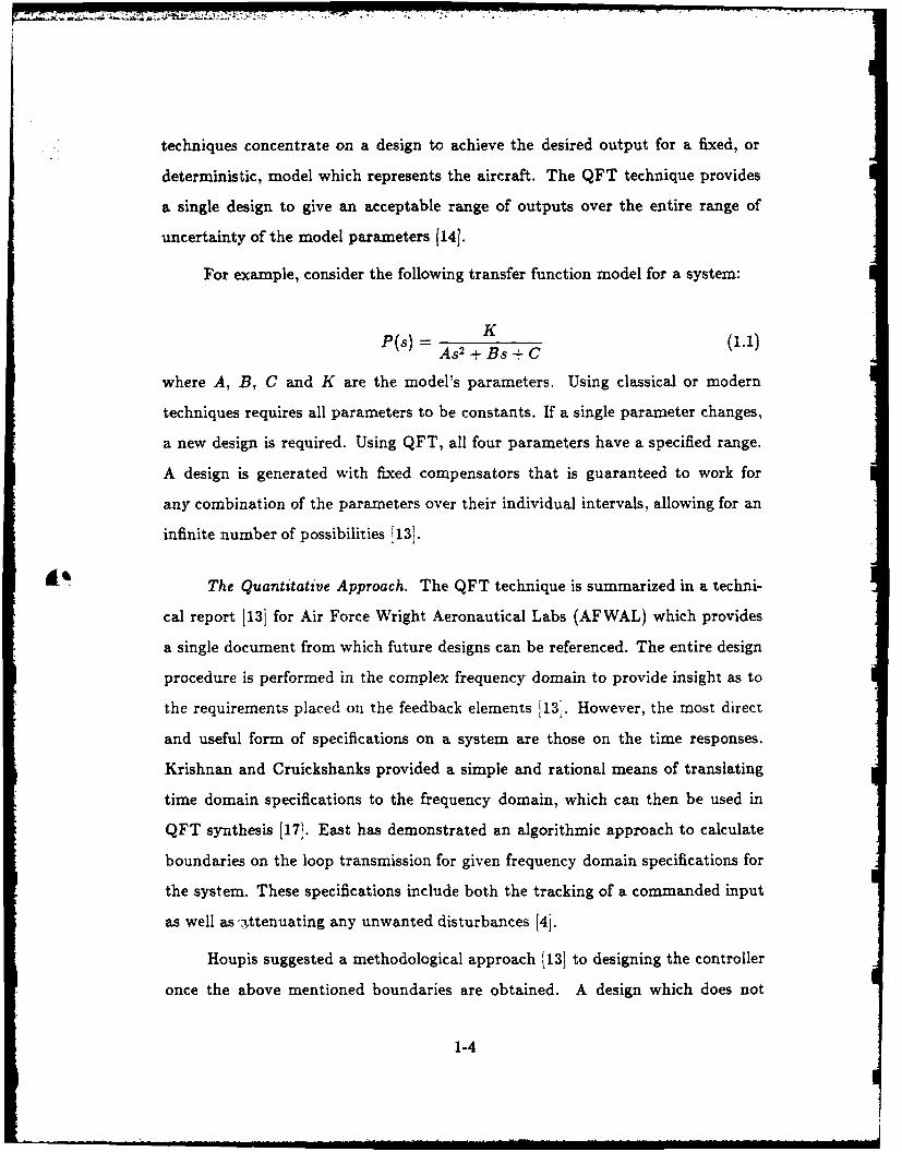
For example, consider the following transfer function model for a system:
g (S.1)F(s) = As 2 + Bs + C
where A, B, C and K are the model's parameters. Using classical or modern
techniques requires all parameters to be constants. If a single parameter changes,
a new design is required. Using QFT, all four parameters have a specified range.
A design is generated with fixed compensators that is guaranteed to work for
any combination of the parameters over their individual intervals, allowing for an
infinite number of possibilities 1131.
The Quantitative Approach. The QFT technique is summarized in a techni-
cal report [13] for Air Force Wright Aeronautical Labs (AFWAL) which provides
a single document from which future designs can be referenced. The entire design
procedure is performed in the complex frequency domain to provide insight as to
the requirements placed on the feedback elements ]13'. However, the most direct
and useful form of specifications on a system are those on the time responses.
Krishnan and Cruickshanks provided a simple and rational means of translating
time domain specifications to the frequency domain, which can then be used in
QFT synthesis [17]. East has demonstrated an algorithmic approach to calculate
boundaries on the loop transmission for given frequency domain specifications for
the system. These specifications include both the tracking of a commanded input
as well as attenuating any unwanted disturbances [4j.
Houpis suggested a methodological approach [13] to designing the controller
once the above mentioned boundaries are obtained. A design which does not
1-4
violate any of the boundaries is guaranteed to meet the desired frequency domain
specifications over the entire range of uncertainty for both tracking and disturbance
attenuation 1131. Once the choice of using quantitative feedback theory has been
made, there exist two logical paths to take - linear or nonlinear synthesis.
Linear Time-Invariant QFT. The simplest application of quantitative feed-
back synthesis is an extension of the current flight control procedures; that is to
take the approximate linear models of the aircraft and replace the constant param-
eters with a range of values. The resulting designs then operate at larger deviations
from the deterministic model.
Although this technique is an improvement over other prominent techniques,
it is still based upon the approximate linear model. However, Hamilton [51 has
shown that a single fixed design can be sufficiently robust to allow for a combi-
nation of total surface failures, yet still maintain the flyability of an unmanned
research vehicle. Simulations of the design included nonlinearities which were not
designed for; however there was no guarantee that the design would work with the
nonlinear elements included. Hamilton noted that the QFT procedure eliminates
the trial and error portion of design, but was still very tedious due to the lack of
computer aided design programs specifically written for QFT design '5. Walke and
Horowitz extended QFT to uncertain MIMO plants whose determinant had right
half plane poles and zeros and, applied it to the experimental X-29 aircraft over
the entire range of uncertainty after contracted designers abandoned the attempt
to independently control two of the output variables [11].
Yaniv has stated that the lack of a generic computer aided design (CAD)
package has kept QFT from being used by industiy; most work is being done
by graduate students 21'. Houpis has noted that AFIT produced ICECAP and
introduced MATRIXx packages are part of an ongoing effort to create a QFT CAD
package but are not as yet complete [141.
1-5
Non-Linear QFT. Horowitz was the first to present a quantitative procedure
of synthesis for nonlinear, time-varying systems with large uncertainty. The work
of Porter and other modern theorists at the time dealt only with the qualitative
properties of nonlinear design [101. Since that time, the theory has continued to
expand and prove itself. Golubev applied the nonlinear QFT technique to control
a modified Air Force F-4 to an angle of attack reaching 35 degrees, an extremely
nonlinear case 18].
The above nonlinear design technique is based on conversion of the nonlinear
models to "equivalent linear" models with the appropriate uncertainty. This could
lead to much larger equivalent linear uncertainty than inherently needed. This is
attributed to the manner in which the "equivalent linear" models were obtained.
Use of nominal nonlinear plant cancellation, involving a nonlinear network of the
same complexity as the plant overcomes this problem [6]. At a chosen nominal plant
value, the combination of the two behaves like a linear time-invariant network for all
Alt inputs and allows the designer to greatly reduce over design [6]. The large "saving"
thereby obtained was vividly demonstrated in a highly nonlinear uncertain 2 x 2
MLMO problem 17].
Barfield points out the need for nonlinear uncertainty models in early flight
control simulations. Current practice is to adjust for the pilot dynamics after the
aircraft is in the advanced simulation testing phase where modifications are expen-
sive [11. QFT may prove to be a valuable design tool when working with nonlinear
pilot models that are highly uncertain. Parameters in such models change, not
only from person to person, but from day to day. Taking this into account early
in the design may account for less need, if any at all, of fine tuning in the later
stages of simulation.
Summary. The foundation has been laid to make the design of a flight control
system quantitative in nature. The technique still requires a large amount of
1-6
designer interaction, resulting in the requirement for a QFT CAD package. The
development of such a package will no doubt increase the use of the technique
throughout the control industry.
Robustness is inherent in QFT. There is no need to examine system ro-
bustness after a design has been made, as is the case in much of modern control
methods.
The nonlinear QFT techniques lend themselves directly to early man-in- the-
loop simulations and may save money in the design process.
Finally, it is obvious that the modern control statement that frequency re-
sponse methods are only valid for linear time-invariant systems, is false [6,7,8,10].
Assumptions
The following assumptions are made in the design problem of this ,hesis.
1. All parameters contain finite uncertainty.
2. All commanded inputs and desired outputs are Laplace transformable.
3. All aircraft models (plants) have a unique inverse. This assumption excludes
the case of hard saturation of elevator deflection.
4. The set of commanded inputs describes the range of the actual inputs to the
aircraft.
5. The design is only in the longitudinal axis, therefore the only independent
command input is the elevator.
It should be noted that assumptions 3 and 5 are added here only to reduce the
scope of the thesis and, in theory, can be relaxed. QFT has been extended to
handle the hard saturation problem, but the usual QFT can be applied only if the
inverse range is finite. For example given an output y(t), there is only a finite
1-7
number of inputs z,(t) which can generate this y(t) [81. In actuality, uncertainty
can be semi-infinite, i.e. a gain factor from 1 to oo but not from -oo to +00 (8].
Scope
The foundation of this thesis is laid in nonlinear quantitative feedback theory.
This thesis applies the technique to a single input, single output (SISO) nonlinear
system with large parameter uncertainty. There is an inner stability augmenta-
tion system (SAS) loop involving a nonlinear airframe model and, an outer loop
containing the pilot, where the model contains a pure time delay.
The full, nonlinear six degrees of freedom equations of motion are used to
generate the plants, although the design is done only for the longitudinal axis.
The only commanded input to the system is a symmetric elevator deflection
and the commanded output is C*: normal acceleration at the pilot station blended
with pitch rate.
The completed design is simulated as a linear system using MATRIXx and
on a Fortran simulator using the six degrees of freedom, nonlinear equations of
motion. The validation of the design is to demonstrate that all of the output
responses are within acceptable limits.
Approach
The first step in the design procedure is to obtain linear time-invariant models
which are rigorously equivalent to the nonlinear plant with respect to the defined
set of desired outputs. These equivalent plants are generated from time histories of
the input and output from simulator data supplied by AFWAL. This data is used
in a program, developed by Golubev [81 and provided by Dr. Horowitz, to generate
linear time-invariant (LTI) plants that are equivalent to the nonlinear plant in that
both models give the same output for the given input. This procedure is repeated
for the set of inputs and outputs that are to exist in the operating region of the
1-8
system. The result is a set of LTI equivalent plants which are used in the design
process.
Next, the boundaries on acceptable outputs provided by AFWAL are trans-
lated from the time domain to the frequency domain. At this point, a decision can
be made whether the specifications are reasonable and attainable by any design
method. QFT or other. The generation of bounds on a nominal loop in the fre-
quency domain are obtained, which must be satisfied in order that the output is in
the acceptable set over the entire set P. When the design is completed without vio-
lating any boundary, the controller is guaranteed to work, not only for the nominal
plant, but also for the entire nonlinear plant set over its range of uncertainty.
The controller design is linearly simulated on MATRIXx as a first validation
and a design tool. The final validation is performed on an existing nonlinear YF-16
simulator using the full six degree of freedom equations.
Presentation
This thesis has seven chapters. Chapter II develops the nonlinear QFT the-
ory. Chapter III presents the generation of the linear time-invariant plants. Chap-
ter IV explains the development of the SAS compensation of the inner loop. Chap-
ter V presents the MATRIXx linear and Fortran nonlinear simulations of the inner
loop excluding pilot compensation. Chapter VI explains the development of the
additional single degree of freedom pilot compensation, as well as its simulation,
while Chapter VII contains the conclusions and recommendations for future study.
Appendix A includes the LTI set P derived from Golubev's program along with
plots validating these transfer functions. Appendix B presents the plant templates
of interest and frequency domain tracking bounds. Appendix C contains simula-
tions of the inner loop SAS along with the data used to obtain the prefilter, while
Appendix D derives the fourth order Pad approximation of a pure time delay used
in the Fortran simulations.
1-9
II. Nonlinear QFT Theory
Introduction
This chapter presents the theory behind controller design for a nonlinear
uncertain plant. A brief overview of linear SISO QFT design is presented. The
reader is referred to a technical report [13] for a comprehensive presentation of the
design process.
Linear SISO Case
In the design of a controller for a linear model the technique begins with a
set of linear differential equations whose parameters are uncertain, giving a set of
plant transfer functions P = {P}. Every possible combination of parameters gives
a different plant contained in the set P.aIt is desired that the final closed loop tracking response be within given
or desired acceptable bounds, for any possible combination of parameters and
therefore any P E P. If the acceptable bounds are given in the time domain they
can be converted to equivalent frequency domain bounds 113'. Once the closed
loop frequency response bounds are obtained, the compensator G(s) of Figure 2.1
is used to insure that the variation in the closed loop response is less than or equal
to that of the bounds. However, this is insufficient to guarantee that the closed loop
tracking response for every P E P lies within the tracking bounds. The prefilter
F(s) of Figure 2.1 is used in this final task.
The designs of the compensators G(s) and F(s) are based upon boundaries
that are derived for a set of frequencies. Similar bounds on G(s) can be obtained for
the response of the system to external disturbances. All of the bounds mentioned
above can be generated manually on the Nichols chart 113 or the same concepts
can be programed on a computer for automation as described in Chapter IV.
2-1
F~s) (S) F(S)
F(s) - Prefilter
G(s) - Compensator
P(s) - Plant
Figure 2.1. QFT Compensaced Block Diagram
Nonlinear SISO Case
The problem with the nonlinear case is at the onset of the design. The
differential equations are nonlinear and therefore transfer functions may not be
used in the usual sense. There exists a set of nonlinear plants 4, due to everyi
possible combination of parameter values. It is still desired that all system outputs
due to realistic inputs lie within an acceptable set .4.
It is necessary to find a set of linear time-invariant plants P that is precisely
equivalent to the nonlinear set W with respect to the acceptable output set A. A
rigorously proven technique for this problem. using Schauder's fixed point theo-
rem, shows that a design meeting specifications for the set P will also satisfy the
nonlinear problem with W 10i.
Direct Analytical Model. For the nonlinear plant of Figure 2.2 having the
input x(t), and the output y(t) is of the form:
2-2
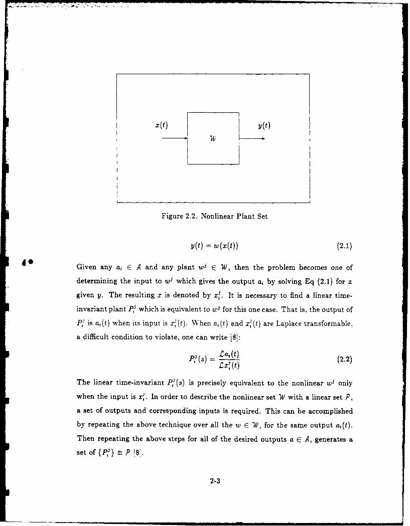
x(t) Y(t)
Figure 2.2. Nonlinear Plant Set
y(t) = w(x(t)) (2.1)
Given any a, E A and any plant wi E W, then the problem becomes one of
determining the input to wi which gives the output ai by solving Eq (2.1) for x
given y. The resulting x is denoted by xj. It is necessary to find a linear time-
invariant plant P/ which is equivalent to w' for this one case. That is, the output of
P/ is a,(t) when its input is x,(t). When a,(t) and xj(t) are Laplace transformable.
a difficult condition to violate, one can write [81:
P/ (s) = La1 (t) (2.2)
The linear time-invariant P/(s) is precisely equivalent to the nonlinear wi only
when the input is x,. In order to describe the nonlinear set W with a linear set P,
a set of outputs and corresponding inputs is required. This can be accomplished
by repeating the above technique over all the w E 14), for the same output ai(t).
Then repeating the above steps for all of the desired outputs a E A, generates a
set of {P} - P [8[.
2-3
Non-Direct Analytical Model. Another technique, based in theory on the
above procedure, is very useful for nonlinear plants that have extremely compli-
cated analytic models. This technique requires either the physical availability of
the plant or a nonlinear simulation of the plant. In this thesis a simulation of
the YF-16 aircraft using the nonlinear equations of motion, complete with a large
data base of aerodynamic data, is used. A stabilizing controller is first obtained,
by "intelligent" cut and try, around the plant with the only goal being that the
acceptable range of outputs can be obtained; no attempt is made at a reasonable
design. The simulator is then run, with the operator supplying the "input" as
needed to obtain one acceptable output. A record is kept of the input signal to the
plant and the plant's output. This can be done by writing the two time histories
to data files. The simulation is repeated until a set of acceptable outputs is ob-
tained that fills the envelope of acceptable responses. The set of plant output and
corresponding input time history points is then used to generate the set of linear
Sequivalent plants P.
Summary
This chapter presents an overview of the continuous SISO QFT design tech-
nique. with extension to the nonlinear case. Two techniques for obtaining the
linear time-invariant equivalent plants are presented, either of which may be used
to accomplish the task.
2-4
I aa irI mI4.I ...i.l.. 4.* .,it,: ., .
III. Derivation of the LTI Equivalent Plants
Introduction
As noted in the previous chapter this thesis does not solve the analytical
model backwards to obtain the linear time-invariant equivalent plants. Instead a
simulator provided by Tom Cord of AFWAL is used. The simulator was originally
developed for studying the high angle of attack and the spin characteristics of the
YF-16.
The Simulator
The following modifications are made to the original simulator in order to
aid in obtaining the desired data:
1. Longitudinal stick force shaping compensation is removed.
2. The commanded output C' is generated as an output variable.
3. Various output files for transfer function generation and MATRIXx graphics
are added.
4. Normal acceleration feedback is replaced with C' feedback.
5. Prefiltering of input signals is added.
The simulator is a Fortran implementation of the actual control laws as well
as the six degree of freedom nonlinear equations of motion for the aircraft. The
aerodynamic derivatives for the equations of motion are supplied from data tables
covering the entire flight envelope, including high angle of attack. During the
simulation, the equations of motion are solved using a Runge-Kutta integration
scheme with the states updated every 5 msec. Reduction of the update interval
shows no improvement in the accuracy obtained as compared to actual flight test
data.
3-1
Each time the simulation is started, a prompt for load factor in g's and angle
of attack in degrees is used to trim the aircraft to its nominal flight condition. This
thesis has the nominal condition of straight and level flight at 0.9M and 20,000 ft
in the derivation of the equivalent plants.
The input to the plant is considered to be the sum of the actuating signals
to the two elevators of Figure 3.1, which are always symmetric since the elevator
is the only commanded input. The output is C* in g's which for the YF-16 is
CG -- A,,= + 12.4q (3.1)
where A,, is the normal acceleration at the pilot station in g's, and q is the pitch
rate in rad/sec. By specifying the above input and output the plant is defined as the
airframe with actuators. including the position and rate limiters of the actuators.
Also included are the dynamics of the aircraft's leading edge flaps of Figure 3.1.
Since this thesis is restricted to a single input, the two available choices are to either
disable the flaps entirely in the trailing position, or make them a dependent input.
The latter is chosen by commanding the leading edge flaps with an angle of attack
plus pitch rate schedule. This not only gives an input totally dependent upon the
commanded elevator input, but also has a stabilizing effect on the aircraft.
The Equivalent Plants
In order to adequately represent 1 with the set P it is necessary to know
the range of acceptable outputs a priori and drive the simulator to outputs that
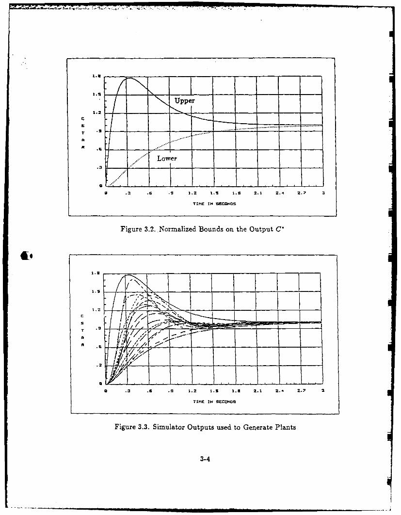
adequately represent that envelope. In Figure 3.2 are the proposed normalized
bounds on a C' response to a step input used in this study. The lower boundary
is modified from that proposed by Tobie [201. The bottom of this envelope does
not allow a higher order response and specifies a minimum greater than zero for
the first 0.2 seconds. This modification makes the lower bound more severe then
the original. The purpose behind the modification is to provide a smoother lower
3-2
Leading Edge FlapsElvtr
Figure 3.1. YF-16 and Control Surfaces
bound on the closed loop response in the frequency domain, as well as to disallow
non-minimum phase responses, with no sacrifice to the time response.
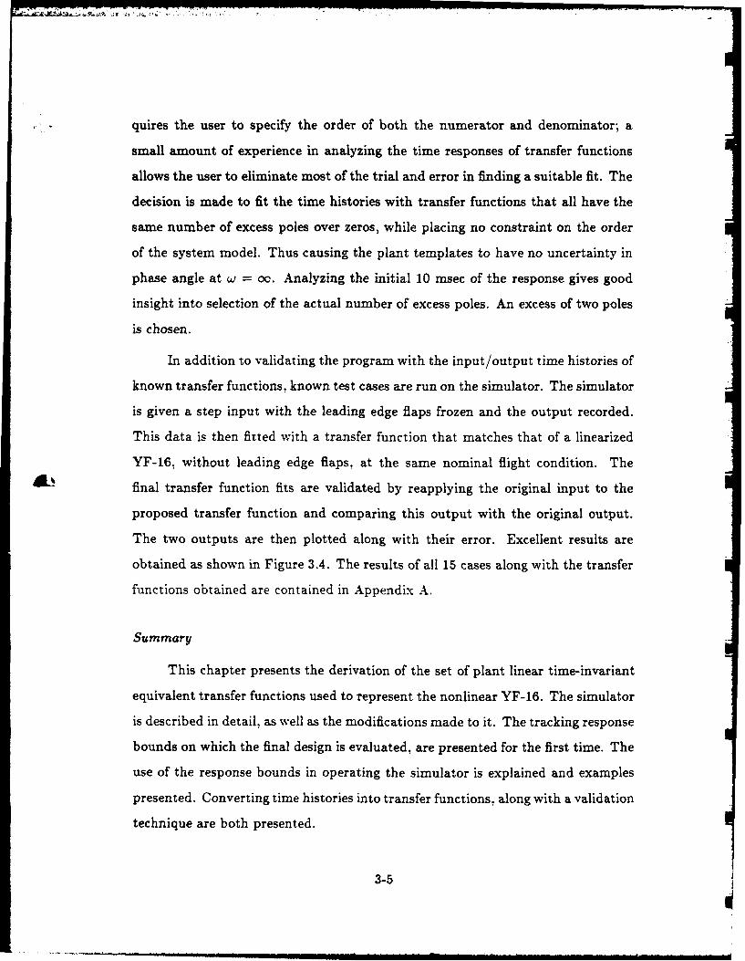
The objective of the simulations is to drive a set of outputs that fill the
envelope of Figure 3.2. This is accomplished with 8 outputs for a 1g envelope
and 7 cases for a 2g envelope, all 15 normalized cases are shown in Figure 3.3
superimposed upon the normalized bounds and are judged to populate them very
well.
The next objective is to find 15 linear time-invariant transfer functions, one
for each input/output pair, given the time histories obtained from the simulator.
Golubev's Fortran subroutine provided by Dr. Isaac Horowitz is used to help ac-
complish this task. By providing a vector of the plant's input, output, and time
of occurrence the subroutine utilizes the Numerical Algorithms Group (NAG) For-
tran Library and Grout's factorization method to obtain a linear transfer function
equivalent to the nonlinear plant for that one specific input. The subroutine re-
3-3
1.21 1
.93 6 1.2 X.S 1.5 2.1 2.4 2.7 3
TIME IN SECONDS
Figure 3.2. Normalized Bounds on the Output C'
1415
a .3 .6 .9 1.2 1.5 1.8 2.1 2.4 2.7
TIME IN SECONDS
Figure 3.3. Simulator Outputs used to Generate Plants
3-4
quires the user to specify the order of both the numerator and denominator; a
small amount of experience in analyzing the time responses of transfer functions
allows the user to eliminate most of the trial and error in finding a suitable fit. The
decision is made to fit the time histories with transfer functions that all have the
same number of excess poles over zeros, while placing no constraint on the order
of the system model. Thus causing the plant templates to have no uncertainty in
phase angle at w = oc. Analyzing the initial 10 msec of the response gives good
insight into selection of the actual number of excess poles. An excess of two poles
is chosen.
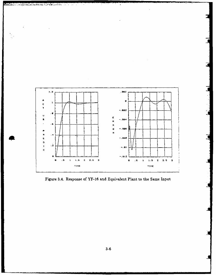
In addition to validating the program with the input/output time histories of
known transfer functions, known test cases are run on the simulator. The simulator
is given a step input with the leading edge flaps frozen and the output recorded.
This data is then fitted with a transfer function that matches that of a linearized
YF-16, without leading edge flaps, at the same nominal flight condition. The
final transfer function fits are validated by reapplying the original input to the
proposed transfer function and comparing this output with the original output.
The two outputs are then plotted along with their error. Excellent results are
obtained as shown in Figure 3.4. The results of all 15 cases along with the transfer
functions obtained are contained in Appendix A.
Summary
This chapter presents the derivation of the set of plant linear time-invariant
equivalent transfer functions used to represent the nonlinear YF-16. The simulator
is described in detail, as well as the modifications made to it. The tracking response
bounds on which the final design is evaluated, are presented for the first time. The
use of the response bounds in operating the simulator is explained and examples
presented. Converting time histories into transfer functions, along with a validation
technique are both presented.
3-5
T
U
SR
.6 R
P 0
R .4 -
a -.S I~ 1 .S 2 2.S 3 G .S I I.s 2 2.5
T IME T IM
Figure 3.4. Response of YF-16 and Equivalent Plant to the Same Input
3-6
IV. Design of the Inner Loop Controller
Introduction
This chapter discusses the design of the compensators F(s) and G(s) shown
in Figure 2.1. The bounds on the nominal loop transmission Lo(s) are modified
slightly from those obtained in the usual QFT problem, due to different responses
obtained from 1g and 2g commands. After the modified bounds are established,
the nominal loop is shaped on the Nichols chart. Once the closed loop is completed,
bounds on the prefilter F(s) are derived and the compensator designed.
Bounds on Lo(s)
The first step in generating the bounds on the nominal loop transmission
is converting the time domain bounds of Figure 3.2 into bounds on the closed
loop response in the frequency domain as shown in Figure 4.1. This is usually
performed using standard figures of merit along with some trial and error; however,
the program used to generate the equivalent plants can also be used.
In obtaining the equivalent plants, it is noted that the 2g responses alone do
not populate an area of the envelope very well due to inertia of the aircraft and use
of the same bounds for 1g and 2g commands. To make the amount of uncertainty
more realistic an additional, more severe, upper bound is placed on the normalized
2g responses (see Appendix B). Since for all cases the output is a minimum phase
response, only the magnitudes of the frequency domain bounds are required to
generate the bounds on Lo(s).
The transfer functions used to model the ig upper bound, 2g upper bound,
and common lower bound are respectively:
15.8965(s + 0.9022) (4.1)(s - 2.6342)(s + 5.439)
4-1
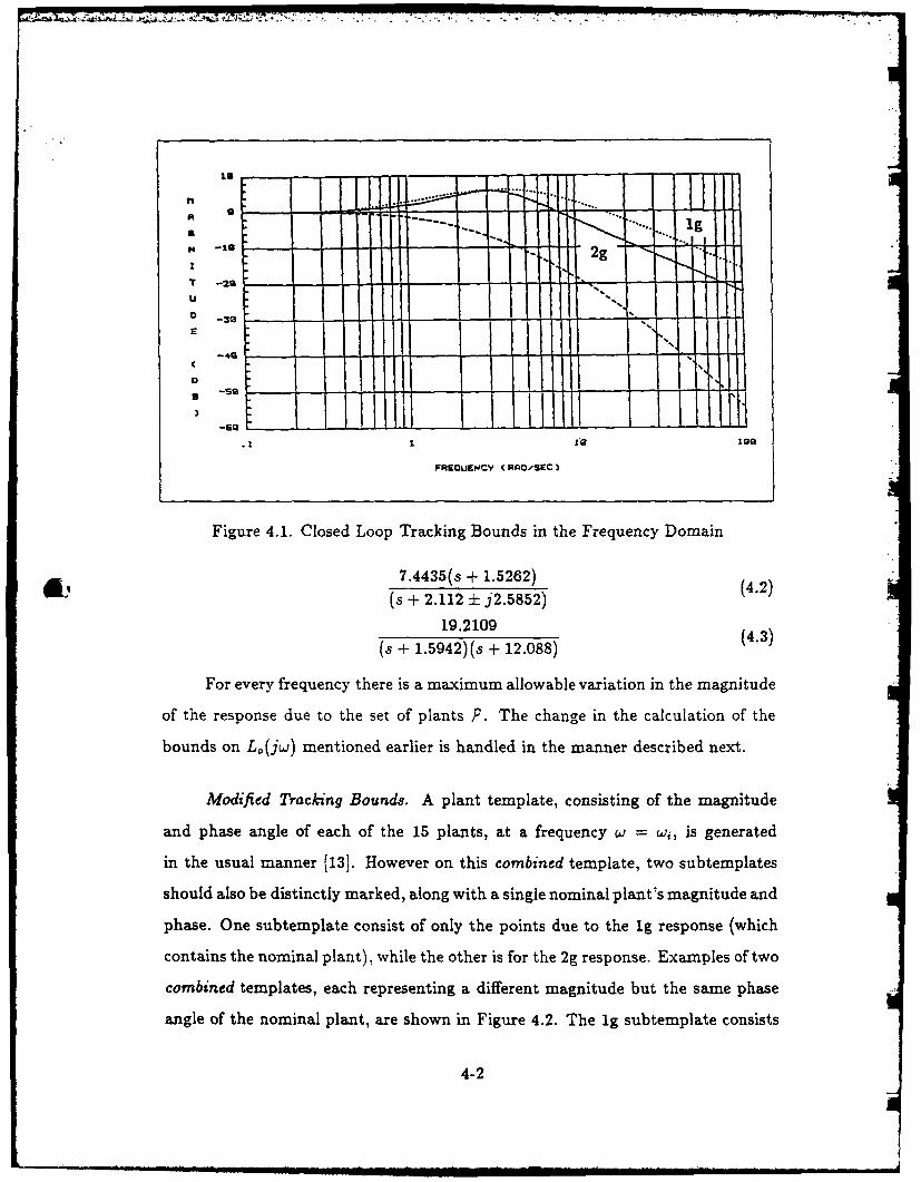
IL1
A 1g
T -219
U S
~~iI ~ a IceUNV 2
FREWEiCY CR$%O.SEC)
Figure 4.1. Closed Loop Tracking Bounds in the Frequency Domain
7.4435(s + 1.5262) (4.2)(s + 2.112 ± j2.5852)
19.2109 (4.3)
(s + 1.5942)(s + 12.088)
For every frequency there is a maximum allowable variation in the magnitude
of the response due to the set of plants P. The change in the calculation of the
bounds on Lo(jw) mentioned earlier is handled in the manner described next.
Modified Tracking Bounds. A plant template, consisting of the magnitude
and phase angle of each of the 15 plants, at a frequency w = wi, is generated
in the usual manner [13]. However on this combined template, two subtemplates
should also be distinctly marked, along with a single nominal plant's magnitude and
phase. One subtemplate consist of only the points due to the 1g response (which
contains the nominal plant), while the other is for the 2g response. Examples of two
combined templates, each representing a different magnitude but the same phase
angle of the nominal plant, are shown in Figure 4.2. The Ig subtemplate consists
4-2
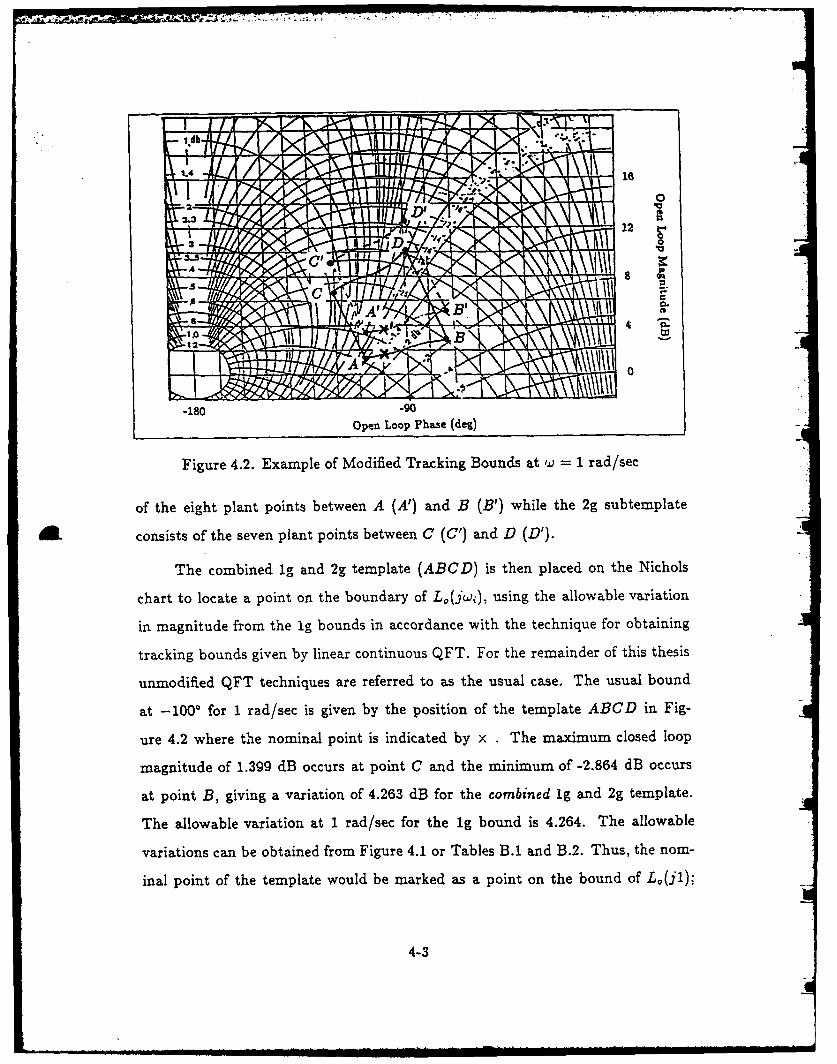
1.48
0
'II
' ly
1. 12
3 0
-180 "goOpen Loop Phase (deg)
91.!
Figure 4.2. Example of Modified Tracking Bounds at ,w = 1 rad/sec
of the eight plant points between A (A') and B (B') while the 2g subtemplate
* consists of the seven plant points between C (C') and D (D').
The combined ig and 2g template (ABCD) is then placed on the Nichols
chart to locate a point on the boundary of L0 (j"w1 ), using the allowable variation
in magnitude from the ig bounds in accordance with the technique for obtaining
tracking bounds given by linear continuous QFT. For the remainder of this thesis
unmodified QFT techniques are referred to as the usual case. The usual bound
at -100 ° for 1 rad/sec is given by the position of the template ABCD in Fig-
ure 4.2 where the nominal point is indicated by x . The maximum closed loop
magnitude of 1.399 dB occurs at point C and the minimum of -2.864 dB occurs
at point B, giving a variation of 4.263 dB for the combined ig and 2g template.
~The allowable variation at 1 rad/sec for the ig bound is 4.264. The allowable
variations can be obtained from Figure 4.1 or Tables B.1 and B.2. Thus, the nom-inal point of the template would be marked as a point on the bound of Lo(j);
4-3
-- •...t.rack.--ing .=- uds gm ienl by lna cotnuu I T Fo th rema Iie of tis thes is
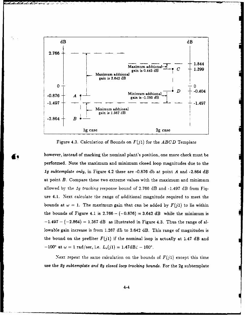
dB dB
2.766 -
-1.844maximum addtoa-j .4
gain is 0.445 dB C 1.399Maximum addtionaI
I gain is 3.642 dB
0 -D -0.404
-0.876 A Minimum addtional Igain is -1.093 dB -
-1.497 ----- 1.497Minimum addtional
gain is 1.367 dB-2.864 - B
Ig case 2g case
Figure 4.3. Calculation of Bounds on F(jl) for the ABCD Template
however, instead of marking the nominal plant's position, one more check must be
performed. Note the maximum and minimum closed loop magnitudes due to the
ig subtemplate only, in Figure 4.2 these are -0.876 db at point A and -2.864 dB
at point B. Compare these two extreme values with the maximum and minimum
allowed by the 1g tracking response bound of 2.766 dB and -1.497 dB from Fig-
ure 4.1. Next calculate the range of additional magnitude required to meet the
bounds at w = 1. The maximum gain that can be added by F(jl) to lie within
the bounds of Figure 4.1 is 2.766 - (-0.876) = 3.642 dB while the minimum is
-1.497 - (-2.864) = 1.367 dB as illustrated in Figure 4.3. Thus the range of al-
lowable gain increase is from 1.367 dE to 3.642 dB. This range of magnitudes is
the bound on the prefilter F(jl) if the nominal loop is actually at 1.47 dB and
-100' at w = 1 rad/sec, i.e. Lo(jl) = 1.47dB/ - 100 ° .
Next repeat the same calculation on the bounds of F(jl) except this time
use the 2g subtemplate and 2g closed loop tracking bounds. For the 2g subtemplate
4-4
the maximum closed loop magnitude is 1.399 dB at point C while the minimum is
-0.404 dB at point D. Figure 4.1 (also see Table B.2) gives the maximum allowable
closed loop magnitude 1.844 dB and the minimum of -1.497 dB. Calculating the
acceptable bounds on F(jl) gives a maximum of 1.844 - 1.399 = 0.445 dB and
a minimum of -1.497 - (-0.404) -- 1.093 dB. Compare the two sets of bounds
on F(jl) thus obtained. The goal of this check is to have one prefilter F(jw) to
meet system specifications. Therefore, if there is some overlap between the two
sets of bounds on F(jwj) there exists a single F(jw) which meets both bounds,
and the boundary location is a valid boundary point of Lo(wi). If there is no
overlap between the two sets of bounds on F(jw,) then the open loop gain must
be increased at this phase value, moving the combined template up the Nichols
chart until an acceptable point is located. For the template ABCD in Figures 4.2
and 4.3 the ranges of 3.642 dB to 1.367 dB and 0.445 dB to -1.093 dB have no
overlap. This is graphically depicted in Figure 4.3 where for the 1g subtemplate
* the minimum increase in gain of 1.367 dB is greater then the maximum allowable
of 0.445 dB for the 2g subtemplate. Therefore, the gain of the plant at -100 ° must
be increased raising the combined template.
If the nominal point of the template is raised to 3.82 dB the template
A'B'C'D' of Figure 4.2 is obt ained. Since the allowable variation is met at the previ-
ous lower gain no additional check is required. Points A' and B' have the closed loop
magnitudes of -0.134 dB and -2.09 dB respectively giving an acceptable ig range
on jF(jl) of 2.766 - (-0.134) = 2.9 dB to -1.497 - (-2.09) = 0.593 dB. Points
C' and D' have the magnitudes 1.248 dB and -0.241 dB respectively giving an ac-
ceptable 2g range on JF(j1) of 1.844 - 1.248 = 0.596 dB to -1.497 - (-0.241) =
-1.256 dB. There now exists an overlap between the ranges on IF(jl), thus
3.82 dB at -100' is a valid boundary point of Lo(jl). This process is repeated
at various values of open loop phase angle for w = 1 radisec and then for various
values of w,.
4-5
Finding the closed loop magnitude M, for the form of Figure 2.1 without
the prefilter F(s), when given the open loop magnitude m and phase angle 6, i.e.
L(jw) = mZP, can be easily automated by solving for the magnitude of the closed
loop transfer function:
WU L(jw) (4.4)IM(Jw)I1 + L(jw)
When both M and m are in arithmetic units not decibels, then
M= m.S+ m2 + 2m cos6 (4.5)
This method is used to obtain the magnitudes of the above example and through
the remainder of this thesis.
Stability Bounds. The modified tracking bounds are obtained for templates
up to a frequency for which the allowable closed loop variation is sufficiently greater
then the variation in the templates's magnitude. In this thesis a frequency of
~*Wh = 10 rad/sec is sufficient. Above this frequency, only stability bounds exist
representing the maximum allowable closed loop magnitude 113]. This thesis uses
a stability or M contour of 3 dB. The boundaries on the nominal loop transmission,
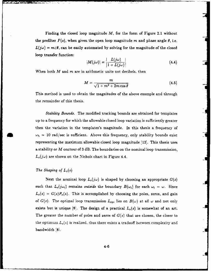
Lo(jw) are shown on the Nichols chart in Figure 4.4.
The Shaping of Lo(s)
Next the nominal loop Lo(jw) is shaped by choosing an appropriate G(s)
such that Lo(jwj) remains outside the boundary B(w,) for each wi = w. Since
Lo(s) = G(s)Po(s). This is accomplished by choosing the poles, zeros, and gain
of G(s). The optimal loop transmission LoPt lies on B(w) at all w and not only
exists but is unique 18. The design of a practical Lo(s) is somewhat of an art.
The greater the number of poles and zeros of G(s) that are chosen, the closer to
the optimum L,(s) is realized, thus there exists a tradeoff between complexity and
bandwidth 8 1.
4-6
L.(jO.1)28
2
20
% 883) 1
0~
S( 0) 8 -2.
-20
8(2) - 2
-22 0 ) 0 -4K15 1 0 - 2 - 0 8 - 40 -200
Open Loop Phase (deg)
Figure 4.4. Bounds B( u) on L,,(j and Response of Proposed Design
4-7
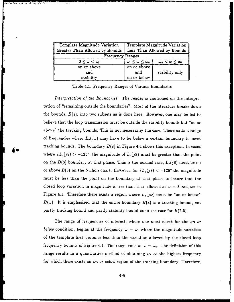
Template Magnitude Variation Template Magnitude VariationGreater Than Allowed by Bounds Less Than Allowed by Bounds
Frequency Ranges0 < W < WW Ul !5 _W< Wh Wh < W < oo
on or above on or aboveand and stability only
stability on or below
Table 4.1. Frequency Ranges of Various Boundaries
Interpretation of the Boundaries. The reader is cautioned on the interpre-
tation of "remaining outside the boundaries". Most of the literature breaks down
the bounds, B(s), into two subsets as is done here. However, one may be led to
believe that the loop transmission must be outside the stability bounds but "on or
above" the tracking bounds. This is not necessarily the case. There exits a range
of frequencies where Lo(jw) may have to be below a certain boundary to meet
tracking bounds. The boundary B(8) in Figure 4.4 shows this exception. In cases
where ZL,(j8) > -1250, the magnitude of L,(j8) must be greater than the point
on the B(8) boundary at that phase. This is the normal case, L0 (j8) must be on
or above B(8) on the Nichols chart. However, for ZL,(j8) < -125' the magnitude
must be less than the point on the boundary at that phase to insure that the
closed loop variation in magnitude is less than that allowed at W = 8 rad,'sec in
Figure 4.1. Therefore there exists a region where Lo(jw) must be "on or below"
B(w). It is emphasized that the entire boundary B(8) is a tracking bound, not
partly tracking bound and partly stability bound as in the case for B(2.5).
The range of frequencies of interest, where one must check for the on or
below condition, begins at the frequency w = w, where the magnitude variation
of the template first becomes less than the variation allowed by the closed loop
frequency bounds of Figure 4.1. The range ends at ., -h. The definition of this
range results in a quantitative method of obtaining Wh as the highest frequency
for which there exists an on or below region of the tracking boundary. Therefore,
4-8
for frequencies above wh only stability bounds exist. These frequency ranges are
summarized in Table 4.1. A quick method to check if a frequency has an on or
below boundary is to place the template at the bottom of the M contour on the
Nichols chart, as if determining stability bounds, and checking the actual variation
in closed loop magnitude. Since the closed loop contours are the closest together
near the 0 dB, -180' point, then this region on the chart is where the largest
variation in the closed loop magnitude exists while meeting the stability bound. If
the closed loop variation is satisfied, the stability bound dominates. If the closed
loop variation is not met, the template on the Nichols chart must be lowered until
the variation is satisfied and the resulting boundary is an "on or below" boundary.
For this thesis the region to check is approximately 3 < w < 10 rad/sec.
Proposed G(s). The first design of G(s) is accomplished using the bounds
on Lo(jw) of Figure 4.4 on page 4-7 with the exception of B(18), and is shown
superimposed upon these bounds. A prefilter F(s) is then designed in the usual
manner [13]. This design is then examined using linear simulation on MATRIXx
by obtaining the responses of each of the 15 LTI plants in P using the fixed G(S)
and F(s). All responses are within the specified boundaries and all except one
are judged to be satisfactory. The response which uses plant 15 has a lightly
damped sinusoidal component of approximately 16 radi sec superimposed upon an
acceptable first order response. Plots of the closed loop frequency responses give
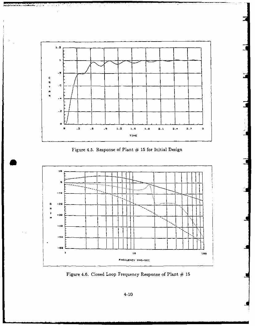
immediate insight into the problem as can be seen in Figures 4.5 and 4.6.
The decision is made to proceed to the nonlinear simulation based upon the
following reasoning. The commanded inputs to the simulator that produced the
time histories to form plant 15 are extremely erratic, worse than any other case. It
is felt that this plant represents a very unlikely operating condition for the aircraft
and is therefore ignored for the time being. The error in this reasoning is that.
the signal to be analyzed in making the judgement of erratic response is the input
signal to the aircraft actuators which, in fact, is rather well behaved. The nonlinear
4-9
T5
.-
A
R
9 .3 .6 .9 1.2 1.S 1.8 2.1 2.4 2.7 3
TIME
Figure 4.5. Response of Plant - 15 for Initial Design
193
__ __ __ '1iT 1 -J.. . ............
G-23 IT -11 A...I....I. I 1
A .
I I I1 19 1 1 1
FREUENCY RmOeSEC
Figure 4.6. Closed Loop Frequency Response of Plant # 15
4-10
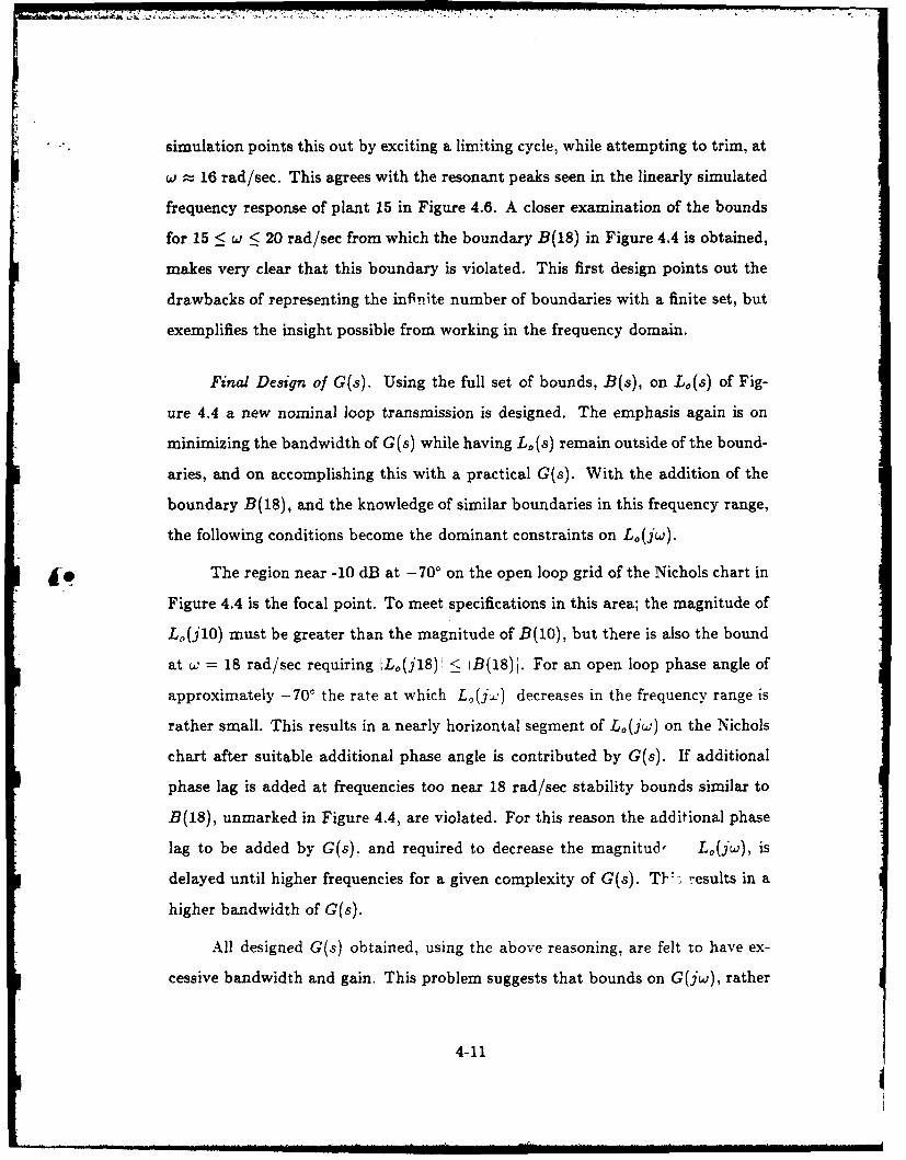
simulation points this out by exciting a limiting cycle, while attempting to trim, at
w = 16 rad/sec. This agrees with the resonant peaks seen in the linearly simulated
frequency response of plant 15 in Figure 4.6. A closer examination of the bounds
for 15 < w < 20 rad/sec from which the boundary B(18) in Figure 4.4 is obtained,
makes very clear that this boundary is violated. This first design points out the
drawbacks of representing the infinite number of boundaries with a finite set, but
exemplifies the insight possible from working in the frequency domain.
Final De8ign of G(s). Using the full set of bounds, B(s), on Lo(s) of Fig-
ure 4.4 a new nominal loop transmission is designed. The emphasis again is on
minimizing the bandwidth of G(s) while having L,(s) remain outside of the bound-
aries, and on accomplishing this with a practical G(s). With the addition of the
boundary B(18), and the knowledge of similar boundaries in this frequency range,
the following conditions become the dominant constraints on Lo(jw).
The region near -10 dB at -70' on the open loop grid of the Nichols chart in
Figure 4.4 is the focal point. To meet specifications in this area; the magnitude of
L,(jlO) must be greater than the magnitude of B(10), but there is also the bound
at w = 18 rad/sec requiring IL(j18)' < B(18) . For an open loop phase angle of
approximately -70c the rate at which L,(j...) decreases in the frequency range is
rather small. This results in a nearly horizontal segment of Lo(jw) on the Nichols
chart after suitable additional phase angle is contributed by G(s). If additional
phase lag is added at frequencies too near 18 rad/sec stability bounds similar to
B(18), unmarked in Figure 4.4, are violated. For this reason the additional phase
lag to be added by G(s), and required to decrease the magnitud- L.(jw), is
delayed until higher frequencies for a given complexity of G(s). T'- -esults in a
higher bandwidth of G(s).
All designed G(s) obtained, using the above reasoning, are felt to have ex-
cessive bandwidth and gain. This problem suggests that bounds on G(jw), rather
4-11
than Lo(jw), give more insight into the problem at hand. Bounds on G(jw) are
obtained by dividing out the nominal plant Po(jw) from the bounds on the nomi-
nal loop transmission Lo(jw), that is G(jw) = 4,and G(s) is designed ratherPo I 3'
than Lo(s). However, the decision is made to continue shaping Lo(s) in the fol-
lowing manner. The major causes of excessive bandwidth and gain of G(s) are the
modified boundaries B(8) and B(10) of Figure 4.4. The normal tracking bounds
at these frequencies for /L(jw) > -100 ° are well below -40 dB. The decision is
therefore made to intentionally violate these two modified bounds (obtained by the
method in the Modified Tracking Bounds subsection of this chapter). The tracking
boundary at B(O.5) now becomes dominant along with the previously mentioned
stability bounds, allowing for a much smaller gain and bandwidth required of G(s).
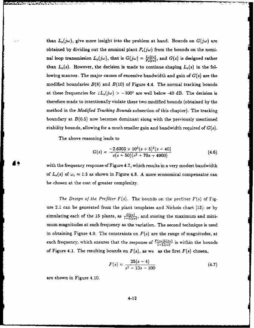
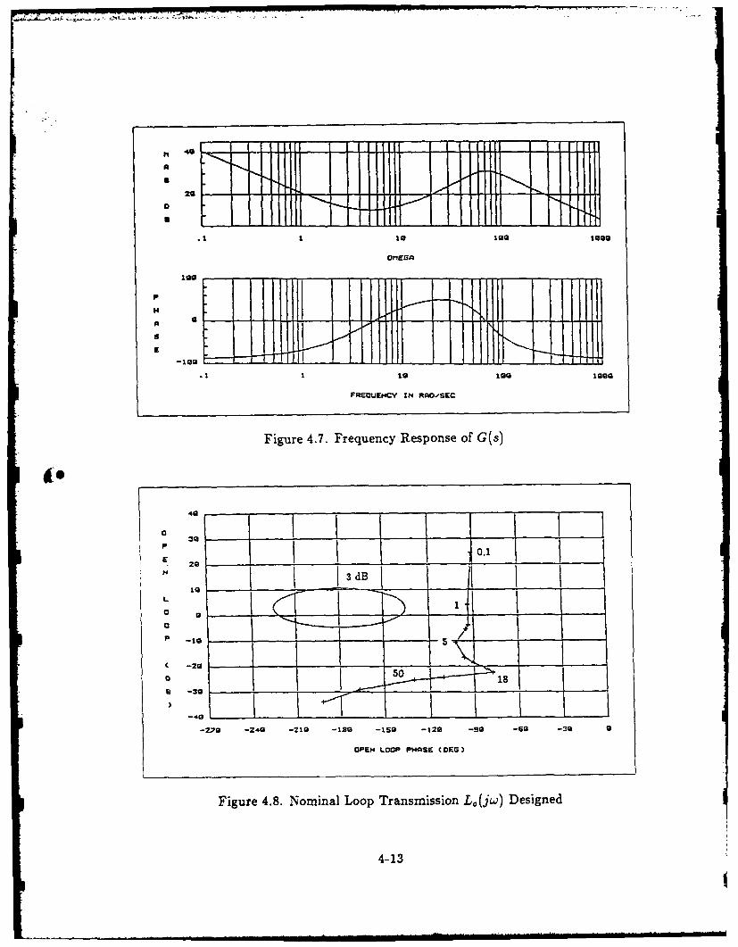
The above reasoning leads to
-2.6303 x 10³ (s + 5)'(s + 40) (4.6)
s (s + 50)(S 2 + 70s + 4900)
io _with the frequency response of Figure 4.7, which results in a very modest bandwidth
of Lo(s) of w, - 1.5 as shown in Figure 4.8. A more economical compensator can
be chosen at the cost of greater complexity.
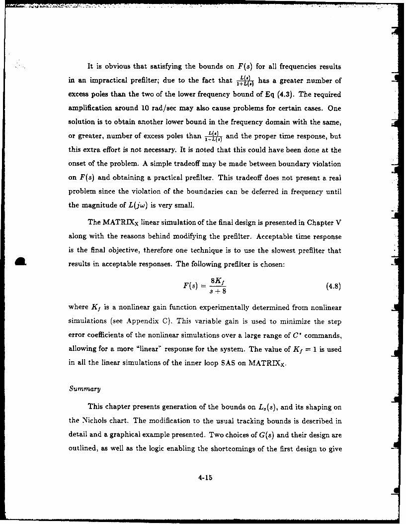
The Design of the Prefilter F(s). The bounds on the prefilter F(s) of Fig-
ure 2.1 can be generated from the plant templates and Nichols chart [13;; or bysimulating each of the 15 plants, as L and storing the maximum and mini-
l+L~jw), d' trn h aiu n ii
mum magnitudes at each frequency as the variation. The second technique is used
in obtaining Figure 4.9. The constraints on F(s) are the range of magnitudes, at
each frequency, which ensures that the response of Fljw)L(is within the bounds
of Figure 4.1. The resulting bounds on F(s), as we- as the first F(s) chosen,
F(s) 25(s+4) (4.7)S2 - JOs - 100
are shown in Figure 4.10.
4-12
'I M'" ..A
logEG
a
S
.1 T 19 199 199G
FREOUENCY IN RAO.-SEC
Figure 4.7. Frequency Response of G(s)
.0.1
E ...
a -30
o 9 __°_ __ .-- '
4-13
19 - ______ __--
i --40
-1 0 .- _ - 1 - - S - 2 - 0 -G _ -
OPEN LOOP PH-ASE C DEO)
Figure 4.8. !Nominal Loop Transmission L0 (jw) Designed
4-13
~ - -sQ . !. .
I.-° . II
_ 1 1 109
PREOUENL'y IN ;:A O/SEC
Figure 4.9. Desired and Actual Variation in Closed Loop Response without F(s)
m is
____ I ii ll 1..............11 ___ __ __ _ __ _ ,_,,_ -II
_ ~I I.i.IIi . -i-..!"ri• .I JIM I-)
-10-1 V I 1
FREUENCY IN RAOSE[C
Figure 4.10. Bounds on Prefilter and Proposed F(jw)
4-14... ...... ... . . . .. . . ,m a m im e n,,,, li nnmn I 1 i 11 I "I -C u INn m AO/SaanEC
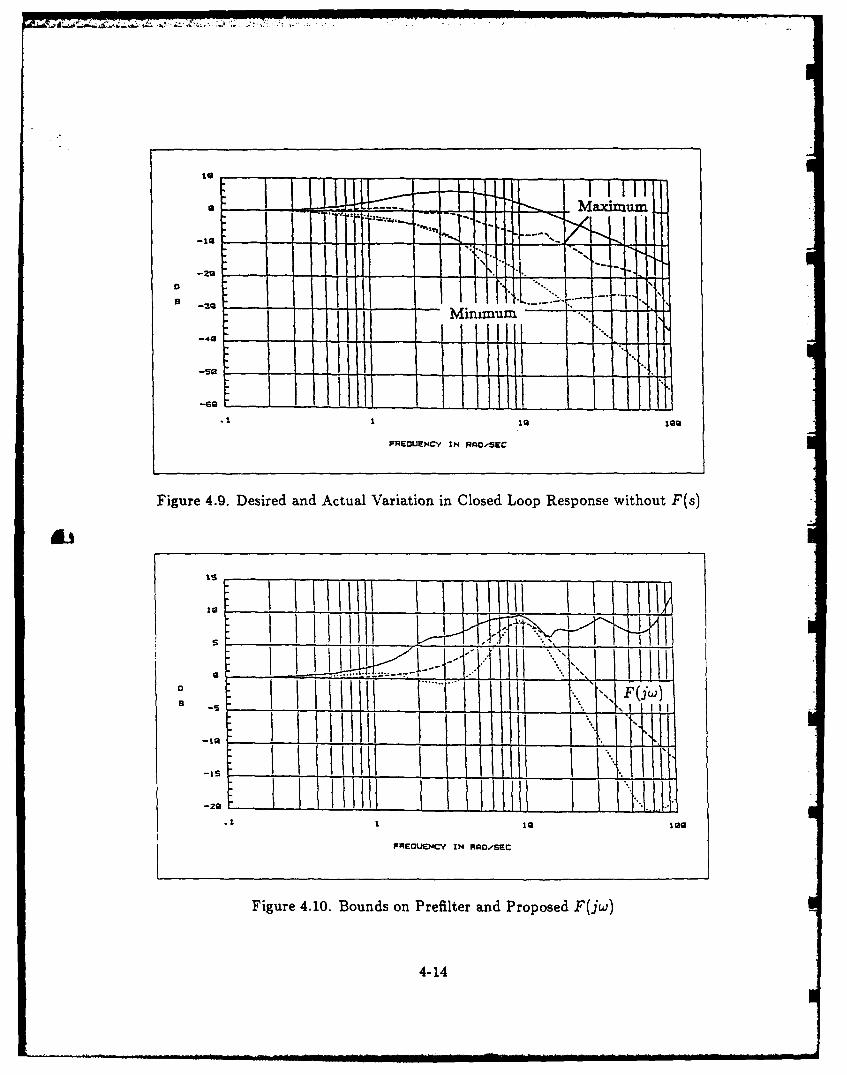
It is obvious that satisfying the bounds on F(s) for all frequencies results
in an impractical prefilter; due to the fact that LI)has a greater number of
1+ ($1
excess poles than the two of the lower frequency bound of Eq (4.3). The required
amplification around 10 rad/sec may also cause problems for certain cases. One
solution is to obtain another lower bound in the frequency domain with the same,
or greater, number of excess poles than L and the proper time response, but1+L~s)
this extra effort is not necessary. It is noted that this could have been done at the
onset of the problem. A simple tradeoff may be made between boundary violation
on F(s) and obtaining a practical prefilter. This tradeoff does not present a real
problem since the violation of the boundaries can be deferred in frequency until
the magnitude of L(jw) is very small.
The MATRIXx linear simulation of the final design is presented in Chapter V
along with the reasons behind modifying the prefilter. Acceptable time response
is the final objective, therefore one technique is to use the slowest prefilter that
A results in acceptable responses. The following prefilter is chosen:
F(s)- 8Kf (4.8)
s+8
where K1 is a nonlinear gain function experimentally determined from nonlinear
simulations (see Appendix C). This variable gain is used to minimize the step
error coefficients of the nonlinear simulations over a large range of C* commands,
allowing for a more "linear" response for the system. The value of Kf = 1 is used
in all the linear simulations of the inner loop SAS on MATRIXx.
Summary
This chapter presents generation of the bounds on L0 (s), and its shaping on
the Nichols chart. The modification to the usual tracking bounds is described in
detail and a graphical example presented. Two choices of G(s) and their design are
outlined, as well as the logic enabling the shortcomings of the first design to give
4-15

needed insight for the accepted second design. Finally, the prefilter is designed and
a discussion on practical prefilters is presented.
4-16
V. Simulation of the Inner Loop SAS
Introduction
This chapter presents the linear and nonlinear simulations of the stability
augmentation system (SAS) designed in Chapter IV. The design only guarantees
satisfaction of responses for ig and 2g C* commands at the nominal flight con-
dition of 0.9M at 20,000 ft; however, the inherent robustness of the technique is
demonstrated by significantly varying the initial conditions. A demonstration of
the linearizing effect of the feedback is included. The inner loop is then modeled as
an equivalent LTI plant for use in the additional pilot compensation of Chapter VI.
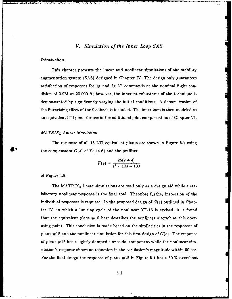
MA TRIXx Linear Simulation
The response of all 15 LTI equivalent plants are shown in Figure 5.1 using
£5 the compensator G(s) of Eq (4.6) and the prefilter
F ( 25(s+4)
F(s) - s2 + lOs + 100
of Figure 4.8.
The MATRIXx linear simulations are used only as a design aid while a sat-
isfactory nonlinear response is the final goal. Therefore further inspection of the
individual responses is required. In the proposed design of G(s) outlined in Chap-
ter IV, in which a limiting cycle of the nonlinear YF-16 is excited, it is found
that the equivalent plant #15 best describes the nonlinear aircraft at this oper-
ating point. This conclusion is made based on the similarities in the responses of
plant #15 and the nonlinear simulation for this first design of G(s). The response
of plant #15 has a lightly damped sinusoidal component while the nonlinear sim-
ulation's response shows no reduction in the oscillation's magnitude within 50 sec.
For the final design the response of plant #15 in Figure 5.1 has a 30 % overshoot
5-1
1.21
7
9 .3 . .9 1.2 I.S 1.9 Z. 1 2.4 2.7 3
TI ME
Figure 5.1. MATRIXx Simulation of SAS Over Range of Uncertainty
and a slight amount of oscillation before reaching its final value, as seen in trace #1
of Figure 5.2. From previous experience with the nonlinear simulation, it is ex-
pected that the response of the nonlinear aircraft would be worse. The decision is
made to slow down the prefilter, specifically to remove the amplification around
10 rad/sec from Figure 4.8. The implementation of the final prefilter. -1- gives
the response of trace -2 in Figure 5.2 for plant #,15. The slower prefilter causes
several of the responses of the set P to violate the bounds on the output; however
the nonlinear results are the end objective. The simulations are then continued
using the first order prefilter.
Nonlinear Simulation
The compensation is then implemented in Fortran in the form of Figure 2.1
page 2-2 where the output of G(s) is the actuating signal to the elevator's actuators
and the feedback signal is C'. The initial flight condition is specified and the
program calculates the required thrust as well as the deflections of the elevators
5-2
-. -- ---- -
1.1.... . ....L .... . . . . .... .......-.- -.
--- -----------
1. I,__ ___.1 24 .
ITIME
i/ ...9 3 9 . . . 1. . , .
Figure 5.2. Response of Plant #15 for the two Prefilters
and leading edge flaps to maintain this condition. Once the equilibrium conditions
C./
are established, the internal states of the compensators are solved for their trim
values. This is automatically completed prior to t = 0. The simulation is then run
where commands are given as perturbations from the trim values and outputs are
in full state values.
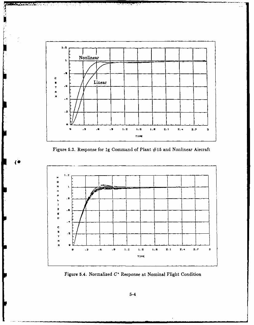
Nominal Flight Condition Simulation. The first run is a ig comnmanded C* at
the nominal flight point of .9M and 20,000 ft, as shown in Figure 5.3. Comparison
of this nonlinear response with the MATRIXX linear response of plant #15 for the
same prefilter validates the use of the first order prefilter for this case. It is yet to
be determined if the slower prefilter adversely affects other operating points.
The design guarantees acceptable responses for Ig to 2g commands at the
nominal flight condition and Figure 5.4 shows this to be the case. The responses
are normalized to the commanded input over the range of 0.5g to 2.5g steps at
increments of 0.1g.
5-3
Io2
Nonlinear
, .. / . .A
.4
. .2
a .3 .6 .9 1.2 1.S 1.3 2.1 2.4 2.7 3
TIME
Figure 5.3. Response for ig Command of Plant #15 and Nonlinear Aircraft
1.Z
0
A rL
I
2
p £
.4
C
S .2T
A
a .3 .6 ,9 1.2 I.S 1.8 2.1 2.4 2.7 3
TIME
Figure 5.4. Normalized C' Response at Nominal Flight Condition
5-4
The nonlinear gain factor, Kf, mentioned in Chapter IV enables the responses
of Figure 5.4 to be normalized to commanded input rather than final value. Prior
to the addition of this gain, the steady state error varied nonlinearly from one
command to another.
It is desired to represent the inner loop SAS as a single linear plant at the
nominal flight condition for synthesis of the outer loop of Chapter VI. Although
the addition of the feedback greatly linearizes the aircraft response, the additional
gain increases the validity of this approximation. The gain Kf is scheduled as a
piece-wise linear function obtained by fitting data points with straight line approx-
imations. Each data point is equal to the magnitude of the command divided by
the steady state value. The function is specifically derived for 0.9M at 20,000 ft
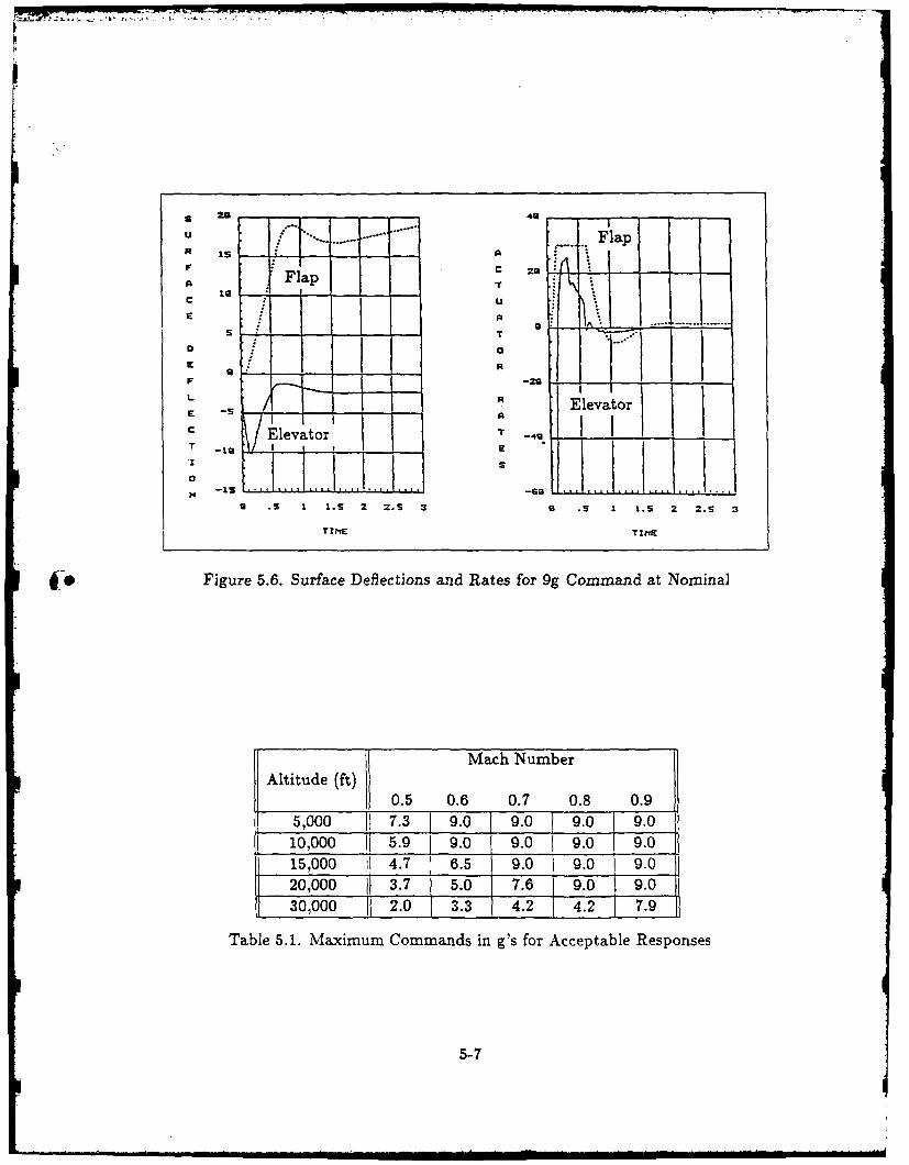
and is contained in Appendix C.
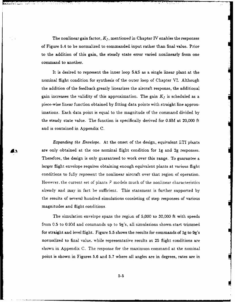
Expanding the Envelope. At the onset of the design, equivalent LTI plants
are only obtained at the one nominal flight condition for ig and 2g responses.
Therefore, the design is only guaranteed to work over this range. To guarantee a
larger flight envelope requires obtaining enough equivalent plants at various flight
conditions to fully represent the nonlinear aircraft over that region of operation.
However, the current set of plants P models much of the nonlinear characteristics
already and may in fact be sufficient. This statement is further supported by
the results of several hundred simulations consisting of step responses of various
magnitudes and flight conditions.
The simulation envelope spans the region of 5,000 to 30,000 ft with speeds
from 0.5 to 0.9M and commands up to 9g's, all simulations shown start trimmed
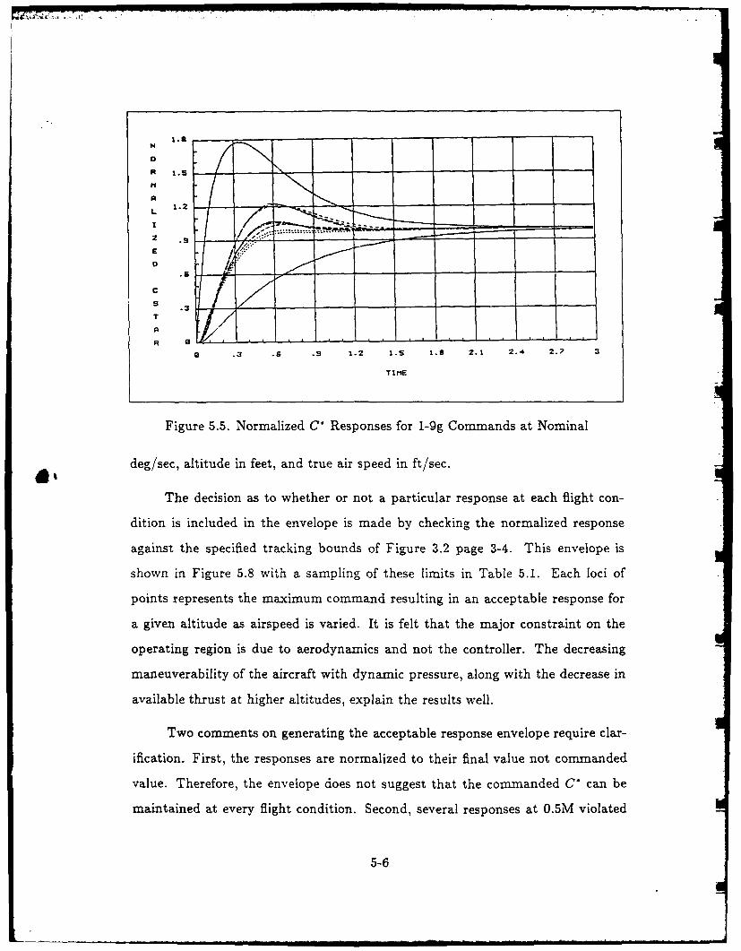
for straight and level flight. Figure 5.5 shows the results for commands of Ig to 9g's
normalized to final value. while representative results at 25 flight conditions are
shown in Appendix C. The response for the maximum command at the nominal
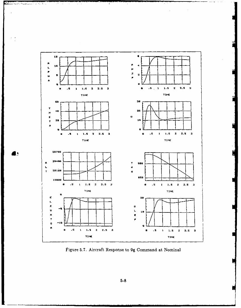
point is shown in Figures 5.6 and 5.7 where all angles are in degrees, rates are in
5-5
1.3
R 1.3
A
L
E
C
A
0 .3 .6 .9 1.2 1-S 1.8 2.1 2.4 2.7 3
TItlE
Figure 5.5. Normalized C' Responses for 1-9g Commands at Nominal
deg/sec, altitude in feet, and true air speed in ft/sec.
The decision as to whether or not a particular response at each flight con-
dition is included in the envelope is made by checking the normalized response
against the specified tracking bounds of Figure 3.2 page 3-4. This envelope is
shown in Figure 5.8 with a sampling of these limits in Table 5.1. Each loci of
points represents the maximum command resulting in an acceptable response for
a given altitude as airspeed is varied. It is felt that the major constraint on the
operating region is due to aerodynamics and not the controller. The decreasing
maneuverability of the aircraft with dynamic pressure, along with the decrease in
available thrust at higher altitudes, explain the results well.
Two comments on generating the acceptable response envelope require clar-
ification. First, the responses are normalized to their final value not commanded
value. Therefore, the envelope does not suggest that the commanded C' can be
maintained at every flight condition. Second, several responses at 0.5M violated
5-6
29 -. 48
R i""
C 2'. / ""-.. .... ...... lalFlap
N - -" A
C ., ..... ," ........
.--. 1'.i .o ; 0
Q : R
F -22
L I ElevatorE - - - -A
SElevator 1-49T -1 I S"-z I S~
9 .S 1 1-5 2 2.S 9 .S 1 1.S 2 2.5 3
4 e Figure 5.6. Surface Deflections and Rates for 9g Command at Nominal
Mach NumberAltitude (ft)
500.5 0.6 0.7 0.8 0.95,000 7.3 9.0 g.0 g.0 9.010,000 5.9 g.0 9.0 1 9.0 9.015,000 I 4.7 6.5 9.0 g.0 9.020,000 I 3.7 5.0 7.6 9.0 9.030,000 2.0 3.3 4.2 4.2 7.9
Table 5.1. Maximum Commands in g's for Acceptable Responses
5-7
is 6
IQ 4L
S S 2 2 Ip P
* .5 1 1.5 2 2.S 3 a .S I 1.5 2 2.S 3
TIME TIME
49 29
. S I I. 2 2.S 3 a .S 1 I.s 2 2.5 3
TIME TI ME
L5 2910
TT 9
2190 0. - s .
a .5 1 1.S 2 2.5 3 a .S 1 1.5 2 2.5 3
TIME TI ME
9
L
E
U L
R9 S5 I 1.5 2 2.5 3 0 S5 1 1.5 2 2.S 3
TIME TIME
Figure 5.7. Aircraft Response to 9g Command at Nominal
5-8
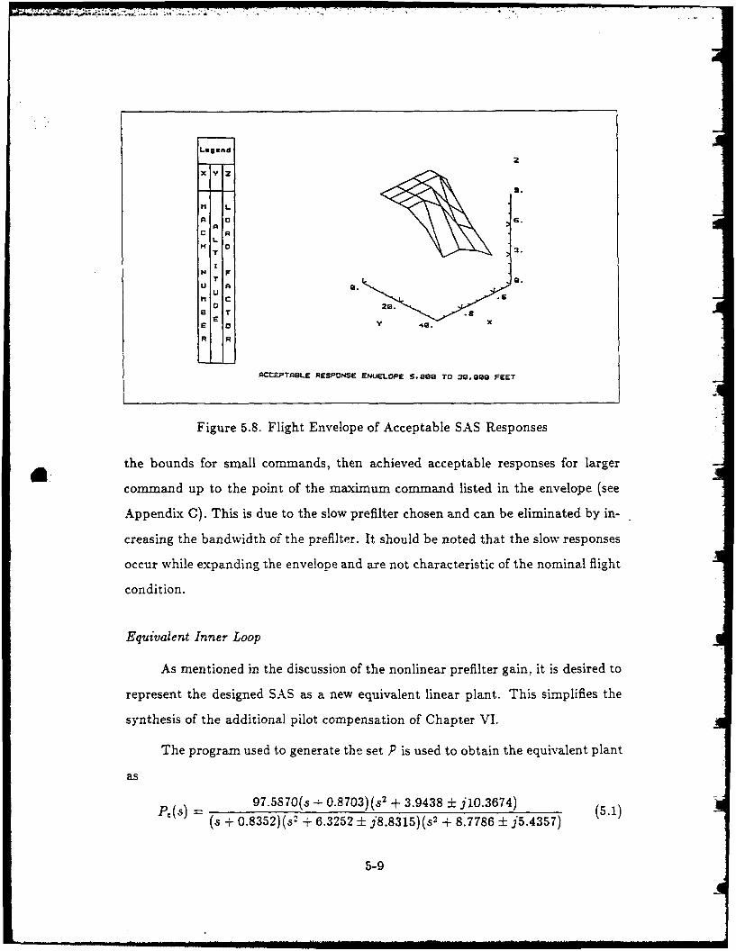
Legend2
II L
A A a..
II A
T .
I
a 0 43. X
R R
ACCEPTABLE RESPONSE ENUELOPE S.90 TO 39.00 FEET
Figure 5.8. Flight Envelope of Acceptable SAS Responses
the bounds for small commands, then achieved acceptable responses for larger
command up to the point of the maximum command listed in the envelope (see
Appendix C). This is due to the slow prefilter chosen and can be eliminated by in-
creasing the bandwidth of the prefilter. It should be noted that the slow responses
occur while expanding the envelope and are not characteristic of the nominal flight
condition.
Equivalent Inner Loop
As mentioned in the discussion of the nonlinear prefilter gain, it is desired to
represent the designed SAS as a new equivalent linear plant. This simplifies the
synthesis of the additional pilot compensation of Chapter VI.
The program used to generate the set P is used to obtain the equivalent plant
as
P, (S) =97.5870(s + 0.8703)(s' + 3.9438 ± j10.3674) (5.1)
(s + 0.8352)(s 2 + 6.3252 ± 3'8.8315)(s 2 + 8.7786 ± j5.4357)
5-9
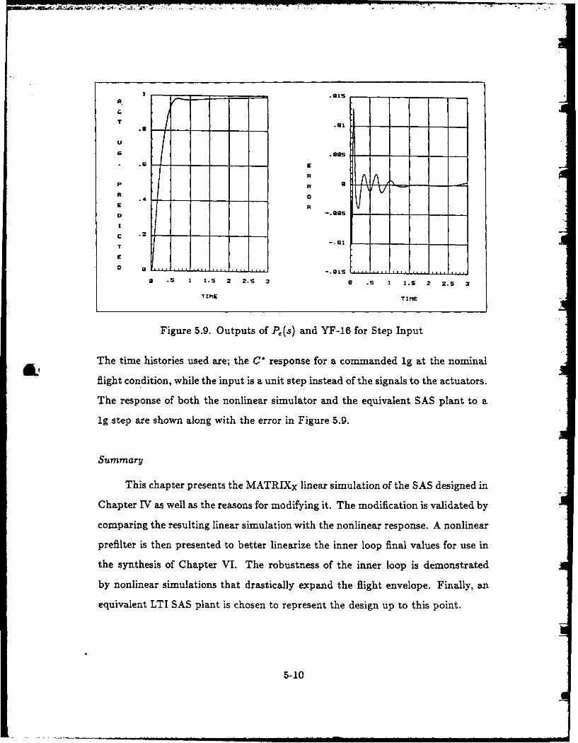
-~ -- - - - ----
GaT .1 -
R
T .91
E
S . .5 2 2.5 3 9 S I 1.5 2 2.S 3
TIME TIME
Figure 5.9. Outputs of P,(s) and YF-16 for Step Input
The time histories used are; the C* response for a commanded ig at the nominal
flight condition, while the input is a unit step instead of the signals to the actuators.
The response of both the nonlinear simulator and the equivalent SAS plant to a
ig step are shown along with the error in Figure 5.9.
Summary
This chapter presents the MATRIXX linear simulation of the SAS designed in
Chapter IV as well as the reasons for modifying it. The modification is validated by
comparing the resulting linear simulation with the nonlinear response. A nonlinear
prefilter is then presented to better linearize the inner loop final values for use in
the synthesis of Chapter VI. The robustness of the inner loop is demonstrated
by nonlinear simulations that drastically expand the flight envelope. Finally, an
equivalent LTI SAS plant is chosen to represent the design up to this point.
5-10
I . . . . .. . . . .. .. . Ip * 1 ,I-. pMw • * -
VI. Pilot Compensation
Introduction
This chapter presents the pilot compensation to be used in conjunction with
the SAS designed in Chapter IV. The synthesis of this compensation is based
upon obtaining a desirable response from the aircraft while reducing the workload
of the pilot. The technique used is based upon the Neal-Smith pilot model for
compensatory tracking. The compensation is designed on MATRIXx followed by
nonlinear simulations in Fortran. A fourth order Pad approximation of a pure
time delay is used in the Fortran simulations and the effects of this approximation
are shown.
The Pilot Model
(0 The form of the mathematical model used in the design of the remaining
compensation is shown in Figure 6.1. The equivalent plant P,(s) is that of Eq (5.1)
representing the SAS designed in Chapter IV. The model used to represent the pilot
is that used in the technical report by Peter Neal and Rodger Smith [18] to predict
pilot ratings for a longitudinal compensatory tracking task. The configuration of
Figure 6.1 allows only a single degree of freedom, Fp(s), to achieve the desired
response.
The dynamic model representing the pilot is taken directly from the Neal-
Smith report (18] as:
~0 .3 , (TiS +1 61Kpe- rp~s + 1)}61
The pilot is represented by a variable gain Kp, a time delay, and a variable first
order compensation network. The factors rp, and rp, represent the adaptive com-
pensation provided by the pilot to accomplish a specific task. The time delay
includes the time required for the pilot to sense a change in C ° , decide what action
6-1
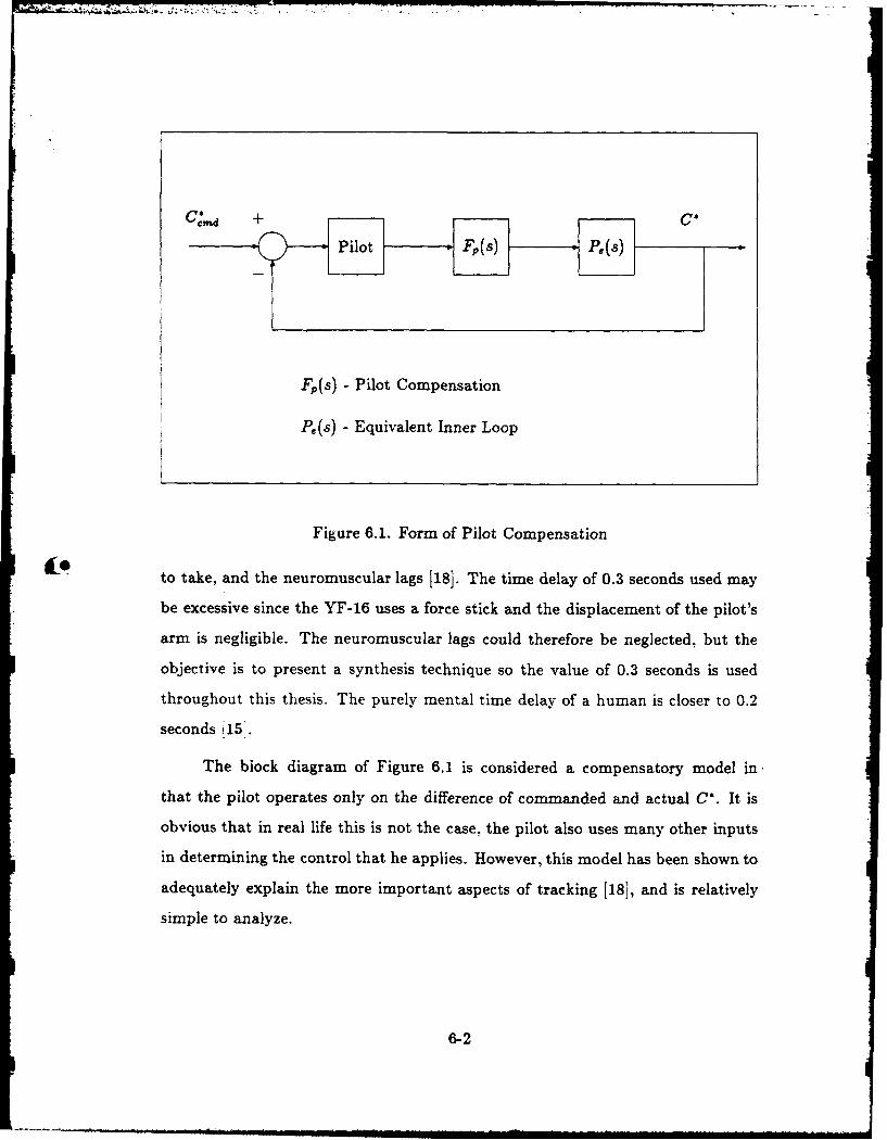
C.,,d + C"
Pilot Fp(s) Ps(s)
Fp(s) - Pilot Compensation
P,(s) - Equivalent Inner Loop
Figure 6.1. Form of Pilot Compensation
to take, and the neuromuscular lags 118]. The time delay of 0.3 seconds used may
be excessive since the YF-16 uses a force stick and the displacement of the pilot's
arm is negligible. The neuromuscular lags could therefore be neglected, but the
objective is to present a synthesis technique so the value of 0.3 seconds is used
throughout this thesis. The purely mental time delay of a human is closer to 0.2
seconds '15'.
The block diagram of Figure 6.1 is considered a compensatory model in-
that the pilot operates only on the difference of commanded and actual C'. It is
obvious that in real life this is not the case, the pilot also uses many other inputs
in determining the control that he applies. However, this model has been shown to
adequately explain the more important aspects of tracking [181, and is relatively
simple to analyze.
6-2
Transforming Analysis to Synthesis
The work in pilot modeling to date has been used to predict the pilot rating
of a designed flight controller; if unacceptable results were predicted, modifications
could be made to the prefilter (1]. The objective of this thesis is to take into ac-
count the prediction of pilot rating, given by the Neal-Smith criterion, and provide
compensation a priori to give an acceptable predicted response.
The goal of this compensation is to minimize the additional compensation, or
workload, required of the pilot to meet good closed loop performance requirements.
The time delay in Eq (6.1) is inherent to the pilot, it is the gain Kp and the first
order compensation network that must be generated by the pilot. Minimizing this
compensation would enable the pilot to act only as a time delay giving, Kp = 1 and
rPI = TP2 -0. The proposed synthesis technique is to perform a prediction analysis
similar to that of Neal-Smith, while forcing an acceptable rating. The resulting
pilot model may be of greater complexity than Eq (6.1) but must contain the time
delay term. The resulting model is then equal to Pilot- Fp(s) of Figure 6.1. Since
it is desired that the pilot provide no additional lead-lag compensation, F,,(s) is
built into the control system and is set equal to the resulting pilot model obtained
above excluding the time delay.
Synthesis of the Pilot Compensation Fp(s)
As outlined earlier, the design of Fp(s) is based upon conducting a prediction
of pilot rating using a modified Neal-Smith criterion. The modification is that
the designer is free to model the pilot with any lead and/or lag compensation,
instead of the "optimum ccmpensaion presented in the technical report [181.
This freedom allows one to obtain an acceptable prediction in cases which would
be impossible with Eq (6.1). This freedom must be weighted against achieving a
practical compensator Fp(s).
6-3
Pilot's View of Good Tracking Performance. The Neal-Smith report [18]
gives an excellent explanation of converting "what the pilot sees" into usable track-
ing performance standards, to which the reader is referred. Sections 6.2 and 6.3 of
the report are summarized below by presenting the performance standards along
with definitions used in the technique 118]. All references to the closed loop are for
C- of Figure 6.1.cd
Bandwidth (.BW): Bandwidth is defined as the frequency for which the phase
angle of the closed loop is equal to -90. It is a measure how quickly the
pilot can move the aircraft's nose towards the target.
Droop: Droop is defined as the maximum excursion of the closed loop magni-
tude below the 0 dB line for frequencies less than WEW. In absence of large
oscillations, droop is a measure of how slowly the aircraft settles down on
target.
Standards of Performance: A minimum bandwidth WBW of 3.5 rad/sec for air-
speeds above those causing wing buffet and a maximum droop of 3 dB.
PIO Tendency: The tendency for pilot induced oscillations is defined in terms of
the Bode magnitude of any closed loop resonant peak that results from the
pilot's efforts to achieve the performance standards.
Pilot Compensation: The pilot's physical and mental workload required to achieve
the standard is defined in terms of the phase angle of his additional compen-
sation at W = WBW.
A visualization of the closed loop standards on bandwidth, droop along with
a PIO limit of 3 dB are shown as closed loop contours on the Nichols chart of
Figure 6.2.
In addition to the above standards of performance, this thesis proposes fur-
ther constraints on the response. These modifications to the standards are gener-
6-4
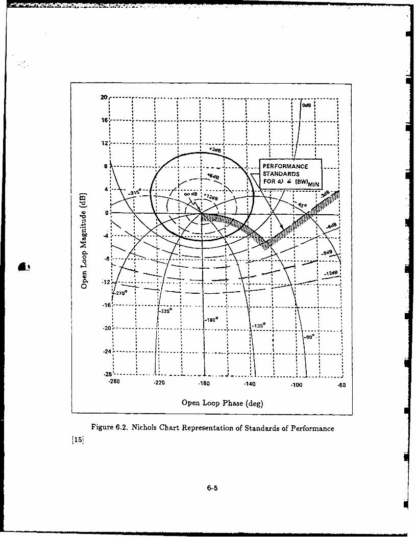
20r --- r --- ------------------ -----------
8-#------------------------ ------ --- PERFORMANCE ------
: --- - . ... 8
4*d STNAD
4$6 ...... ...... .00-6
cOpedopPhs dg
Fiue620ihl hr ersntto fSadrso efrac
-1625
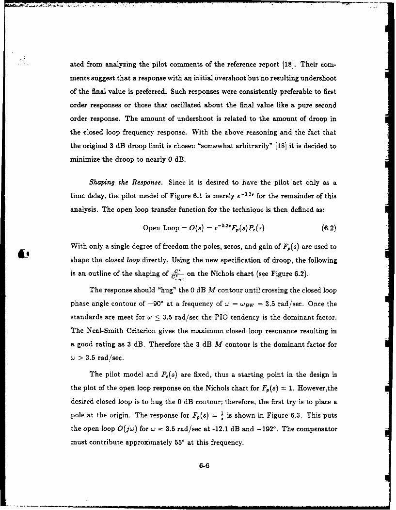
ated from analyzing the pilot comments of the reference report [18]. Their com-
ments suggest that a response with an initial overshoot but no resulting undershoot
of the final value is preferred. Such responses were consistently preferable to first
order responses or those that oscillated about the final value like a pure second
order response. The amount of undershoot is related to the amount of droop in
the closed loop frequency response. With the above reasoning and the fact that
the original 3 dB droop limit is chosen "somewhat arbitrarily" 118] it is decided to
minimize the droop to nearly 0 dB.
Shaping the Response. Since it is desired to have the pilot act only as a
time delay, the pilot model of Figure 6.1 is merely e-0 .3' for the remainder of this
analysis. The open loop transfer function for the technique is then defined as:
Open Loop = 0(s) = e-0 '3'F(s)P.(s) (6.2)
With only a single degree of freedom the poles, zeros, and gain of Fp(s) are used to
shape the closed loop directly. Using the new specification of droop, the following
is an outline of the shaping of C on the Nichols chart (see Figure 6.2).C:.d
The response should "hug" the 0 dB M contour until crossing the closed loop
phase angle contour of -90' at a frequency of w = WBW = 3.5 rad/sec. Once the
standards are meet for w < 3.5 rad/sec the PIO tendency is the dominant factor.
The Neal-Smith Criterion gives the maximum closed loop resonance resulting in
a good rating as 3 dB. Therefore the 3 dB M contour is the dominant factor for
w > 3.5 rad/sec.
The pilot model and P(s) are fixed, thus a starting point in the design is
the plot of the open loop response on the Nichols chart for Fp(s) = 1. However,the
desired closed loop is to hug the 0 dB contour; therefore, the first try is to place a
pole at the origin. The response for Fp(s) I is shown in Figure 6.3. This putsS
the open loop 0(jw) for w = 3.5 rad/sec at -12.1 dB and -1920. The compensator
must contribute approximately 55' at this frequency.
6-6
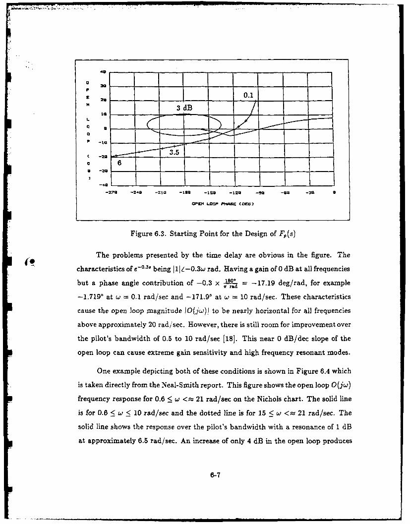
4.
29 Y0ll4 3dB
L
S 6P -3g
-279 -240 -210 -1.Q -ISO - 12 -sQ -6 -30 0
OPEN LOOP PHASE (DEG)
Figure 6.3. Starting Point for the Design of F,(s)
The problems presented by the time delay are obvious in the figure. The
characteristics of e-0° 3s being 1 Z -0.3w rad. Having a gain of 0 dB at all frequencies
but a phase angle contribution of -0.3 x - -17.19 deg/rad, for example
-1.719' at w = 0.1 rad/sec and -171.90 at w = 10 rad/sec. These characteristics
cause the open loop magnitude )O(Jw)! to be nearly horizontal for all frequencies
above approximately 20 rad/sec. However, there is still room for improvement over
the pilot's bandwidth of 0.5 to 10 rad/sec [181. This near 0 dB/dec slope of the
open loop can cause extreme gain sensitivity and high frequency resonant modes.
One example depicting both of these conditions is shown in Figure 6.4 which
is taken directly from the Neal-Smith report. This figure shows the open loop O(jw)
frequency response for 0.6 < w <; 21 rad/sec on the Nichols chart. The solid line
is for 0.6 < w < 10 rad/sec and the dotted line is for 15 < w <; 21 rad/sec. The
solid line shows the response over the pilot's bandwidth with a resonance of 1 dB
at approximately 6.5 rad/sec. An increase of only 4 dB in the open loop produces
6-7
---k ------
16 -- -- r -- -- r -- - -r- - - - - - - - - -1 1
12 ---- r ---- ----- ---- -- - - ------* a a a a a a
-- - --- - - --- -- - -- - - -- N_ I. r - -I
I~~~ I S S I
4 ---- a-------
0 0
a S S S I I I I 2
1 --- ------------- -------- --------- a a a
02
o 12: -- - -- - --- - - ---
2700a
SEON PAS (AT
-- -- a- - - -- -- r - - - - - - - - -
r ------------------------------------------- ------ ------ ------ ----- --
-2 a-- -- - - a - - - a - - - -- - -
-250 -220 -190 -140 -100 .60
Open Loop Phase (deg)
Figure 6.4. Response Showing Cause of High Frequency Resonance
[15]
6-8
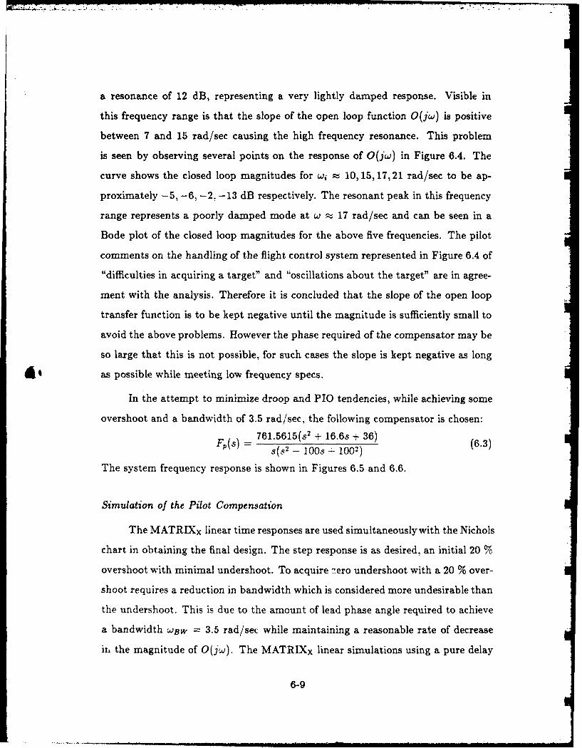
a resonance of 12 dB, representing a very lightly damped response. Visible in
this frequency range is that the slope of the open loop function O(jw) is positive
between 7 and 15 rad/sec causing the high frequency resonance. This problem
is seen by observing several points on the response of O(jw) in Figure 6.4. The
curve shows the closed loop magnitudes for wi z 10, 15, 17, 21 rad/sec to be ap-
proximately -5, -6, -2. -13 dB respectively. The resonant peak in this frequency
range represents a poorly damped mode at w - 17 rad/sec and can be seen in a
Bode plot of the closed loop magnitudes for the above five frequencies. The pilot
comments on the handling of the flight control system represented in Figure 6.4 of
"difficulties in acquiring a target" and "oscillations about the target" are in agree-
ment with the analysis. Therefore it is concluded that the slope of the open loop
transfer function is to be kept negative until the magnitude is sufficiently small to
avoid the above problems. However the phase required of the compensator may be
so large that this is not possible, for such cases the slope is kept negative as long
4* as possible while meeting low frequency specs.
In the attempt to minimize droop and PIO tendencies, while achieving some
overshoot and a bandwidth of 3.5 rad/sec, the following compensator is chosen:
Fp(s) = 761.5615(s + 16.6s + 36) (6.3)s(s2 - 100s - 1002)
The system frequency response is shown in Figures 6.5 and 6.6.
Simulation of the Pilot Compensation
The MATRIXx linear time responses are used simultaneously with the Nichols
chart in obtaining the final design. The step response is as desired, an initial 20 %
overshoot with minimal undershoot. To acquire z:ero undershoot with a 20 % over-
shoot requires a reduction in bandwidth which is considered more undesirable than
the undershoot. This is due to the amount of lead phase angle required to achieve
a bandwidth WBW = 3.5 rad/sec while maintaining a reasonable rate of decrease
irL the magnitude of O(jw). The MATRIXx linear simulations using a pure delay
6-9
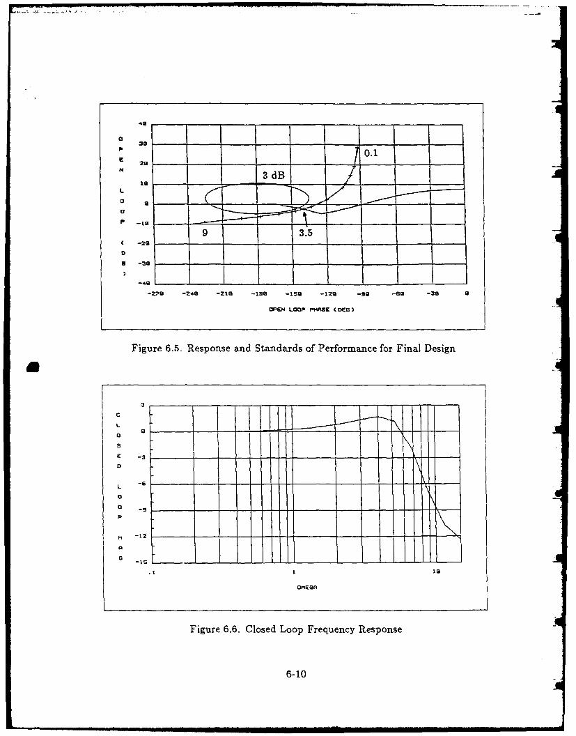
30
P 0.129 ___
3 3dBI I I I
L
0 J
0
-279 -249 -219 -199 -ISO -129 -99 -69 -39
OPEN LOOP PHASE (DES)
Figure 6.5. Response and Standards of Performance for Final Design
C
E -3
0
OMEGA
Figure 6.6. Closed Loop Frequency Response
6-10
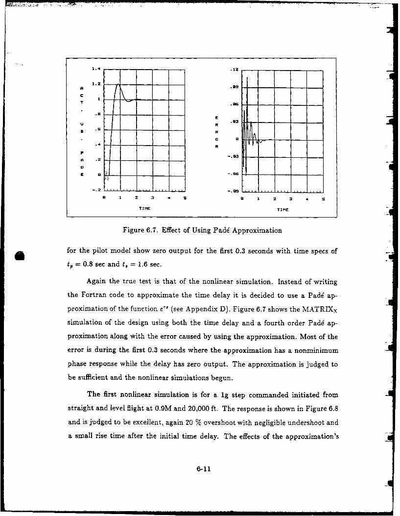
1.4 .1
1.2-
C I
S - R0 6 - -
P .4 R-
DE L:
2 3 4 S 1 2 3
TIME TIME,
Figure 6.7. Effect of Using Pad6 Approximation
~~for the pilot model show zero output for the first 0.3 seconds with time specs of -tP = 0.8 sec and t, = 1.6 sec.
Again the true test is that of the nonlinear simulation. Instead of writing
the Fortran code to approximate the time delay it is decided to use a Pad6 ap-
proximation of the function el (see Appendix D). Figure 6.7 shows the MATRIXx
simulation of the design using both the time delay and a fourth order Pad6 ap-i
proximation along with the error caused by using the approximation. Most of the
error is during the first 0.3 seconds where the approximation has a nonminimum
phase response while the delay has zero output. The approximation is judged to
be sufficient and the nonlinear simulations begun.
The first nonlinear simulation is for a 1g step commanded initiated from
straight and level flight at 0.9M and 20,000 ft. The response is shown in Figure 6.8
and is judged to be excellent, again 20 % overshoot with negligible undershoot and
a small rise time after the initial time delay. The effects of the approximation's
6-11
R!P -.. .. 03 -n -nn p - -
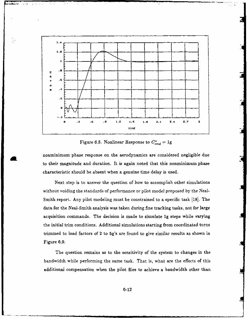
1.4 ,,-
1.2-
.8 ,. -
C
S
T .-
A
R *-
.2- --- -
9 .3 .6 .9 1.2 I-S 1.8 2.1 2.4 2.7 3
TIME
Figure 6.8. Nonlinear Response to Cm.d 1g
£ nonminimum phase response on the aerodynamics are considered negligible due
to their magnitude and duration. It is again noted that this nonminimum phase
characteristic should be absent when a genuine time delay is used.
Next step is to answer the question of how to accomplish other simulations
without voiding the standards of performance or pilot model proposed by the Neal-
Smith report. Any pilot modeling must be constrained to a specific task [181. The
data for the Neal-Smith analysis was taken during fine tracking tasks, not for large
acquisition commands. The decision is made to simulate ig steps while varying
the initial trim conditions. Additional simulations starting from coordinated turns
trimmed to load factors of 2 to 5g's are found to give similar results as shown in
Figure 6.9.
The question remains as to the sensitivity of the system to changes in the
bandwidth while performing the same task. That is, what are the effects of this
additional compensation when the pilot flies to achieve a bandwidth other than
6-12
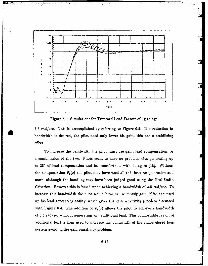
1.4
1.2 - -. "
S .T -/a
R .4 ___ _-,
-.2 - -
2 .3 .- .9 1.2 I.S 1.8 2.1 2.4 2.7 3
TIME
Figure 6.9. Simulations for Trimmed Load Factors of ig to 5gs
3.5 rad/sec. This is accomplished by referring to Figure 6.5. If a reduction in
bandwidth is desired, the pilot need only lower his gain, this has a stabilizing
effect.
To increase the bandwidth the pilot must use gain, lead compensation, or
a combination of the two. Pilots seem to have no problem with generating up
to 250 of lead compensation and feel comfortable with doing so I18]. Without
the compensation Fr(s) the pilot may have used all this lead compensation and
more, although the handling may have been judged good using the Neal-Smith
Criterion. However this is based upon achieving a bandwidth of 3.5 rad/sec. To
increase this bandwidth the pilot would have to use mostly gain, if he had used
up his lead generating ability, which gives the gain sensitivity problem discussed
with Figure 6.4. The addition of Fp(s) allows the pilot to achieve a bandwidth
of 3.5 rad/sec without generating any additional lead. This comfortable region of
additional lead is then used to increase the bandwidth of the entire closed loop
system avoiding the gain sensitivity problem.
6-13
Summary
This chapter presents the design of the outer loop of Figure 6.1, consisting
of pilot compensation based upon the Neal-Smith Criteria. The objective of min-
imizing the compensation required of the pilot is accomplished by providing the
compensation, to achieve a bandwidth of 3.5 rad/sec with a good response, with
Fp(s). This allows the pilot to act as a pure time delay. The nonlinear simulations
presented, using a Pad6 approximation of the time delay, show excellent results for
initial load factors of up to 5gs. Finally, a discussion of the effects of bandwidth
show that the closed loop bandwidth for the tracking task has been increased.
61
6-14
VII. Conclusions and Recommendations
Discussion
This thesis demonstrates the application of Nonlinear Quantitative Feedback
Theory to flight control design and presents a compensation design technique which
reduces pilot work load. The nonlinear QFT technique is applied to the YF-16
aircraft which results in an inner loop SAS to control the output C* and guarantees
that the response lies within the bounds suggested by Tobie 120]. However, this
inner loop design does not include the characteristics of the human pilot a priori,
and such is the case with nearly all current preliminary flight control designs [1].
The characteristics of the human pilot are usually not dealt with until the man-
in-the-loop simulation phase of final control system design. Waiting until this
late point in the system's development to attack this problem is extremely cost
inefficient in two ways. First, due to the high cost of such simulations delay must be
keep to a minimum. Secondly, modifications to a system so far into it's development
are very costly. Ignoring the inherent time delay of the human pilot results in
extensive adjustments to the original design to achieve satisfactory pilot ratings.
Instead of fine tuning the design during this expensive phase of system design:
an adjustment is made prior to these man-in-the-loop simulations with additional
pilot compensation. This pilot compensation allows the controller to achieve good
handling qualities predictions for simulations including the inherent time delay of
the human pilot.
Extensive use of CAD tools, not included in this thesis, greatly reduces the
calculations and book keeping required in the synthesis process. Listings of the
Fortran code and MATRIXx routines may be made available through the following
points of contact:
7-1
Convert Time Histories to Transfer Functions: Professor Isaac M. Horowitz,
Department of Electrical Engineering and Computer Sciences, University of
California at Davis.
MATRIXx Macros: Professor Constantine H. Houpis, Electrical and Computer
Science Engineering Department, Air Force Institute of Technology, WPAFB
Dayton Ohio.
Conclusions
Based upon the work performed on this thesis and the results obtained, the
following conclusions are made.
1. A nonlinear plant can be represented by a set P of linear time-invariant plants
for use in a design problem. The method of Chapter III is found to describe
the nonlinear YF-16 rather well.
2. Nonlinear Quantitative Feedback Theory can be successfully applied to the
synthesis of flight controllers resulting in fixed compensators that yield ac-
ceptable responses over a large range of nonlinear parameter variation.
3. Linear simulations are an effective design aid but final analysis of the control
of the nonlinear plant must be performed using the nonlinear simulations.
The linear simulations are invaluable for the insight that they provide but this
insight can only be gained by comparing them to the nonlinear simulations.
4. Use of the MATRIXx routines in the synthesis process greatly reduces the
workload and calculation errors, however they are written for this specific
thesis. There is a definite need for a generic computer aided design (CAD)
package to ease the design burden associated with QFT and to speed the
design process.
5. It is possible to design compensation for the task of reducing pilot workload
and therefore increasing the system bandwidth. The technique developed
7-2
in this thesis will work for other tasks. It is necessary to emphasize that
the closed loop performance requirements are task specific, and the expected
performance is expected to vary depending on the particular task.
Recommendations
After completion of the of the stability augmentation system design for the
YF-16 and the pilot compensation, followed by analyzing the simulation results,
one task remains to be completed. The technique must be validated by actual
man-in-the-loop simulations such as on AFIT's SIMSTAR hybrid computer. The
real-time, full flight envelope simulator is nearing completion (2,16]. An original
objective of this thesis effort was to include such simulations; however, upgrades to
the system have prevented it. Beyond this immediate suggested task, three distinct
areas for future study are proposed.
1. Extend the nonlinear SISO plant to that of the nonlinear MIMO plant with
an emphasis on survivability and on acceptable responses while experienc-
ing various surface failure conditions. Such work is underway based upon
linearized plant models; however, using the nonlinear plant should make the
results more realistic.
2. Expand the area of pilot compensation. Given any existing flight controller,
use the developed technique for a variety of pilot tasks, where each task has
different performance requirements. The controller can be adapted for a given
task and a new compensator designed. Included in this research should be the
ability to perform real-time man-in-the-loop simulations such as on AFIT's
SIMSTAR F-16 simulator. This type of simulation can validate the technique
proposed in this thesis by comparing handling qualities ratings for the same
aircraft before and after the implementation of the pilot compensation for
different tasks.
7-3
3. Develope a generic interactive CAD package devoted to QFT. Many useful
routines have been developed by researchers for their work; however, their
objective is to complete a specific design. Therefore these routines are written
for the specific problem at hand with no time to check out other possibilities
that can arise in other situations. A full time effort devoted solely to such a
CAD package will be a step in the right direction.
Summary
This chapter reviews the design and results of this thesis. Recommendations
are made for future projects in nonlinear QFT, pilot compensation, and develop-
ment of a QFT CAD package.
7-4
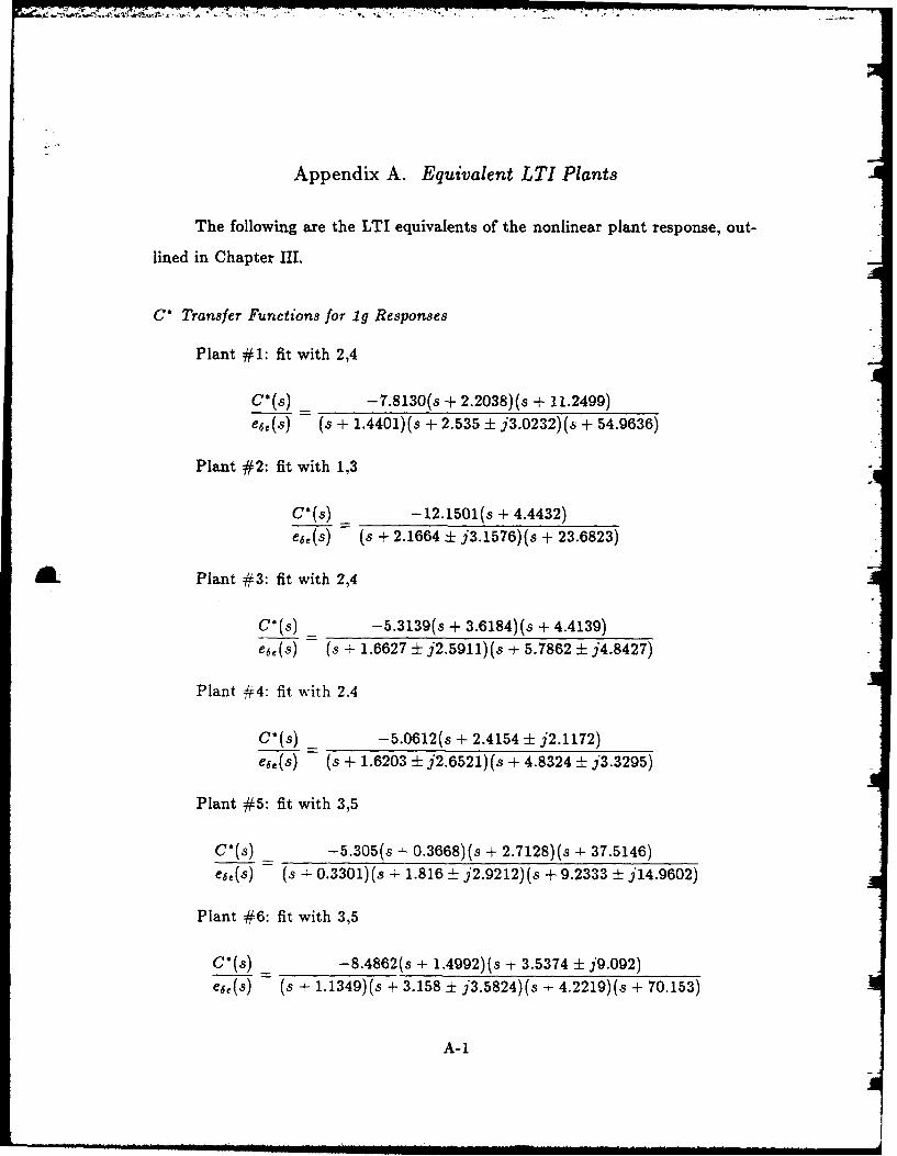
Appendix A. Equivalent LTI Plants
The following are the LTI equivalents of the nonlinear plant response, out-
lined in Chapter III.
C" Transfer Functions for ig Responses
Plant #1: fit with 2,4
C(.) _ -7.8130(s + 2.2038)(s + 11.2499)e6,e(s) (s + 1.4401)(s + 2.535 ± j3.0232)(s + 54.9636)
Plant #2: fit with 1,3
C'(s) _ -12.1501(s + 4.4432)e6,(s) (s + 2.1664 ± j3.1576)(s + 23.6823)
ft Plant #3: fit with 2,4
C'(s) _ -5.3139(s + 3.6184)(s + 4.4139)e6,(s) (s + 1.6627 ± j2.5911)(s + 5.7862 ± j4.8427)
Plant #4: fit with 2.4
C'(s) - -5.0612(s + 2.4154 ± j2.1172)
e6e(s) (s + 1.6203 ± j2.6521) (s + 4.8324 ± j3.3295)
Plant #5: fit with 3,5
C(s) _ -5.305(s -- 0.3668)(s + 2.7128)(s + 37.5146)
e6e(s) (s + 0.3301)(s - 1.816 ± j2.9212)(s + 9.2333 ± j14.9602)
Plant #6: fit with 3,5
C'(s) -8.4862(s + 1.4992)(s + 3.5374 ± j9.092)e6e(s) (s + 1.1349)(s + 3.158 ± j3.5824)(s -t 4.2219)(s + 70.153)
A-1
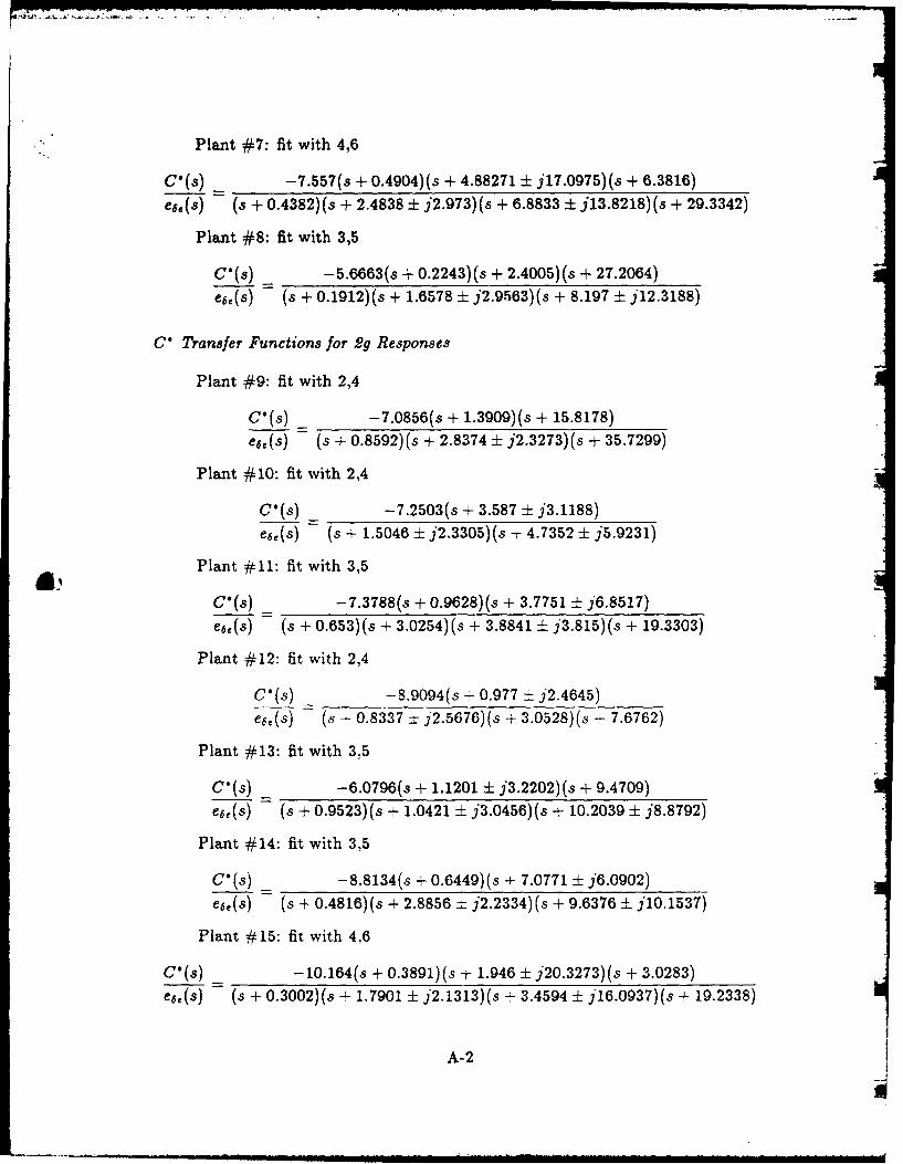
Plant #7: fit with 4,6
C*(s) -7.557(s + 0.4904) (s + 4.88271 ± j17.0975) (s + 6.3816)e6e(s) (s + 0.4382)(s + 2.4838 ± j2.973)(s + 6.8833 ± j13.8218) (s + 29.3342)
Plant #8: fit with 3,5
CO(s) _ -5.6663(s + 0.2243)(s + 2.4005) (s + 27.2064)
e6e(s) (s + 0.1912) (s + 1.6578 ± j2.9563)(s + 8.197 ± j12.3188)
C" Transfer Functions for 2g Responses
Plant #9: fit with 2,4
C*(s) _ -7.0856(s + 1.3909) (s + 15.8178)e6,(s) (s + 0.8592)(s + 2.8374 ± j2.3273)(s + 35.7299)
Plant #10: fit with 2,4
C*(s) _ -7.2503(s + 3.587 ± j3.1188)e,,(s) (s + 1.5046 ± j2.3305)(s + 4.7352 ± j5.9231)
Plant #11: fit with 3,5
C*(s) = -7.3788(s + 0.9628)(s + 3.7751 ± j6.8517)e6,(s) (s + 0.653) (s + 3.0254) (s + 3.8841 ± j3.815)(s + 19.3303)
Plant #12: fit with 2,4
CO(s) -8.9094(s - 0.977 - j2.4645)
e6.(5) (s - 0.8337 , j2.5676)(s + 3.0528)(s -- 7.6762)
Plant #13: fit with 3.5
C'(s) _ -6.0796(s + 1.1201 ± j3.2202)(s + 9.4709)e6e(s) (s + 0.9523) (s + 1.0421 ± j3.0456)(s + 10.2039 ± j8.8792)
Plant #14: fit with 3,5
C'(s) _ -8.8134(s + 0.6449) (a + 7.0771 ± j6.0902)
e6,(s) (s + 0.4816) (s + 2.8856 : j2.2334)(s + 9.6376 ± j1O.1537)
Plant #15: fit with 4,6
C*(s) -10.164(s + 0.3891)(s + 1.946 ± j20.3273)(s + 3.0283)e6,(s) (s + 0.3002)(s + 1.7901 ± j2.1313)(s -- 3.4594 ± j16.0937)(s + 19.2338)
A-2
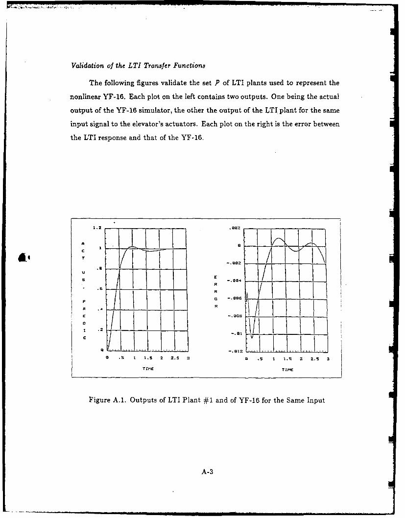
Validation of the LTI Transfer Functions
The following figures validate the set P of LTI plants used to represent the
nonlinear YF-16. Each plot on the left contains two outputs. One being the actual
output of the YF-16 simulator, the other the output of the LTI. plant for the same
input signal to the elevator's actuators. Each plot on the right is the error between
the LTI response and that of the YF-16.
T 17 1-.2 , -I I ii
C
* '?* .t..... ... JJ ' I ''Ii L L ] r' *',..1.S 2 2.S - 9 S 1 1.. 2 2. -.
Figure A.1. Outputs of LTI Plant #1 and of YF-16 for the Same Input
A-3
R!
.. . .. .. . "-',' - ., ,,,,,, wm~ a ~ n an m ~ lm im ll l| N ai i lll I. ... . . .,R
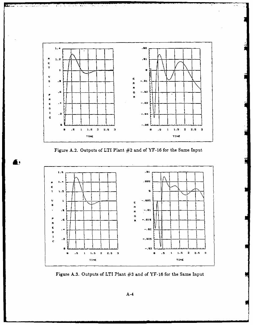
1.2 .92
s1.2 2 1 .1 -1..
'T I 0. I_
P a -. 22-
II A I I I1
S~R1 .6 2 1
a .s 1 I.S 2 2.S 3 G .S I 1.5 2 2.S 3
TIME TI MtiE
Figure A.2. Outputs of LTI Plant #2 and of YF-16 for the Same Input
4._,
1.A .0 ,9
C I 1--U 1 -. ; 177.
P SR -. 91tS __ _
.2 \ J ,/
ZELL-. .|
9 .5 1 1.5 2 2.5 3 9 .5 1 1.5 2l 2.5 3
TI ME TU E;
Figure A.3. Outputs of LTI Plant #3 and of YF-16 for the Same Input
A-4
R 1
,~~~ ~ s,,I1 .i n II IIl I Is 2 2.S 3 aI s I I 2- 3
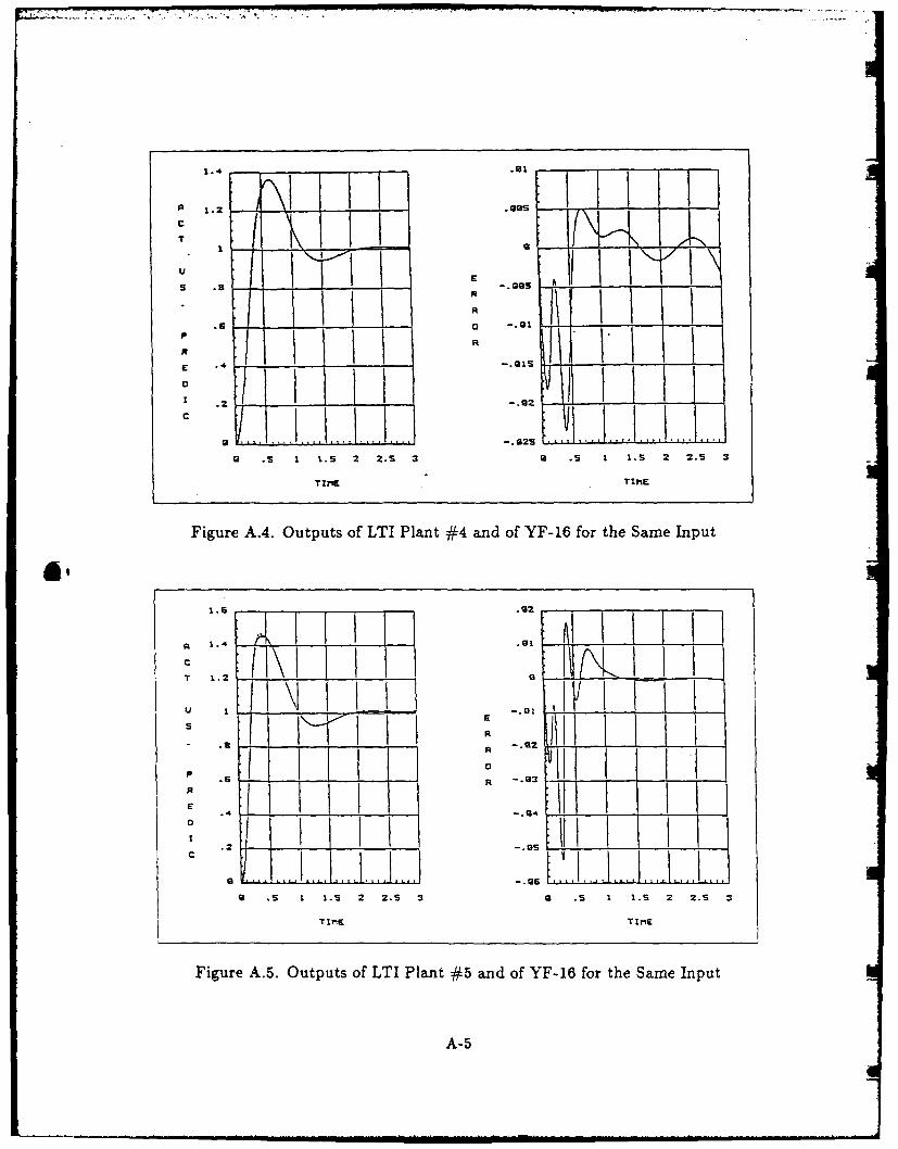
1.2 Gas I I-- .i: '., : ,,:. .:L ,,.I.i , •. . , r r
CI 1
6* I y9~T I. -.G9SS... _.. " !
o : i 11 .2 . -. 92
9 .5 1 1.S 2 2.S 3 a .5 1 1.s 2 2.S 3
TIME TME
Figure A.4. Outputs of LTI Plant #4 and of YF-16 for the Same Input
' U
1.4 . 4.9
I'\] I =. - - 01 ___.
I A- - I I.. I I-I '
C I III ] -'I jl l --
a 1s 1.s 2 2.S 3 .S I I.S 2 2.S 3
TIME TIME
Figure A.5. Outputs of LTI Plant #5 and of YF-16 for the Same Input
A-5
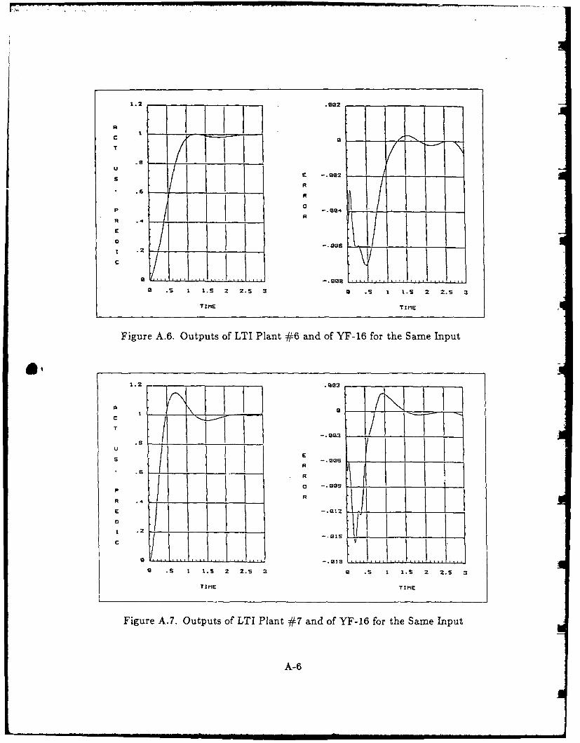
1.2 . 902I
A I° --T
5-
SLLi4-
R
.5 R
P t. IG
R .2-. 008 .E
a .5 L I.S 2 2.5 3 0 .5 1 1.5 2 2.5 3
TT ME TIME
Figure A.6. Outputs of LTI Plant #6 and of YF-16 for the Same Input
1.2 ... 0 2 13
I LT -. 003
UES
R .4]R .61,, ,, 7iI.2 :::
. 1 .S 2 2.S 3 Q . 1 1.5 2 2.1 3
TIME TIME
Figure A.7. Outputs of LTI Plant #7 and of YF-16 for the Same Input
A-6
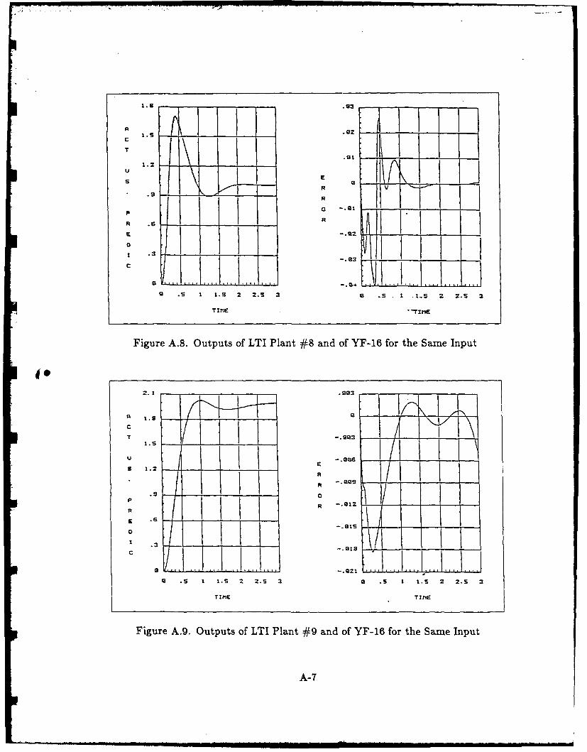
YA1.2 11]
° \ I
SR- ' R
F. o -.91.J IR
R .
c a LKL
9 .S 1 1.5 2 2.5 3 9 .2.5 3
TIME '-TIME
Figure A.8. Outputs of LTI Plant #8 and of YF-16 for the Same Input
2.1 .9 -3
1.9 Q
S1.5 R
P R
F£ .6 ! 1 -*
.3 -. G1s
I . 1 1.9 2 2.9 3 a .S I 1.5 2 2.5 3
TIME T IMEs
Figure A.9. Outputs of LTI Plant #9 and of YF-16 for the Same Input
A-7
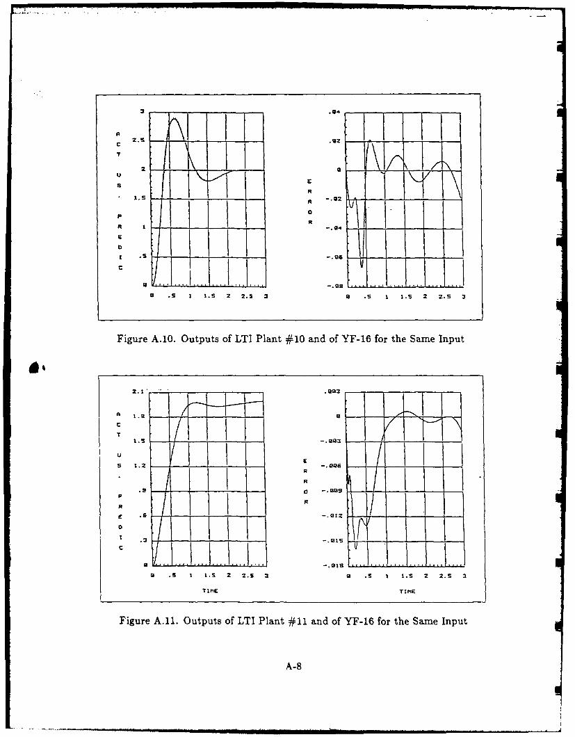
: .s ii Q2.. . i •I
TI 2
U *P IS.0
cRI . - - -. 92 1.
C -. 98 _
S qL /,. I
. I 1 1.5 2 2.S 3 a -S I 1.5 2 2.5 3
Figure A.10. Outputs of LTI Plant #10 and of YF-16 for the Same Input
2.1 - .93
A -.-
E
-.5 -.
~R-.a - . 0 0 9
Rm
R
£ . - - . 9 1 2
1 .3 -. 1IS
S .&.L.L.S l.L 4..LV-.018a S I 1.5 2 2.S 3 a .S 1 1.S 2 2.S 3
TIME TIME
Figure A.11. Outputs of LTI Plant #11 and of YF-16 for the Same Input
A-B
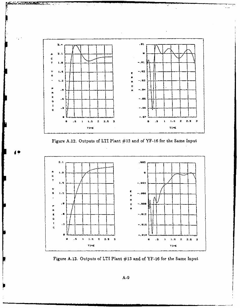
- .i - -
2.4 ~9
A 2.1 - - - -
c
U I.s -. 02
.2-.92P i0
. R -.- 4
-a9s
1 .3 -. 06 --
a .s 1 I.S 2 2.S 3 a .s 1 1.5 2 2.5 3
TI E TIM E
Figure A.12. Outputs of LTI Plant #12 and of YF-16 for the Same Input
2.1
A 1.E
S 1.2 .06
R
R
.9 0
0 .
1 .3 - . 1 s
a s5 I 1.s 2 2.S53 S.1 ... JI 1s2 2.s 3
TIME TI mE
Figure A.13. Outputs of LTI Plant #13 and of YF-16 for the Same Input
A-9
-p- i i i a , i -,,.
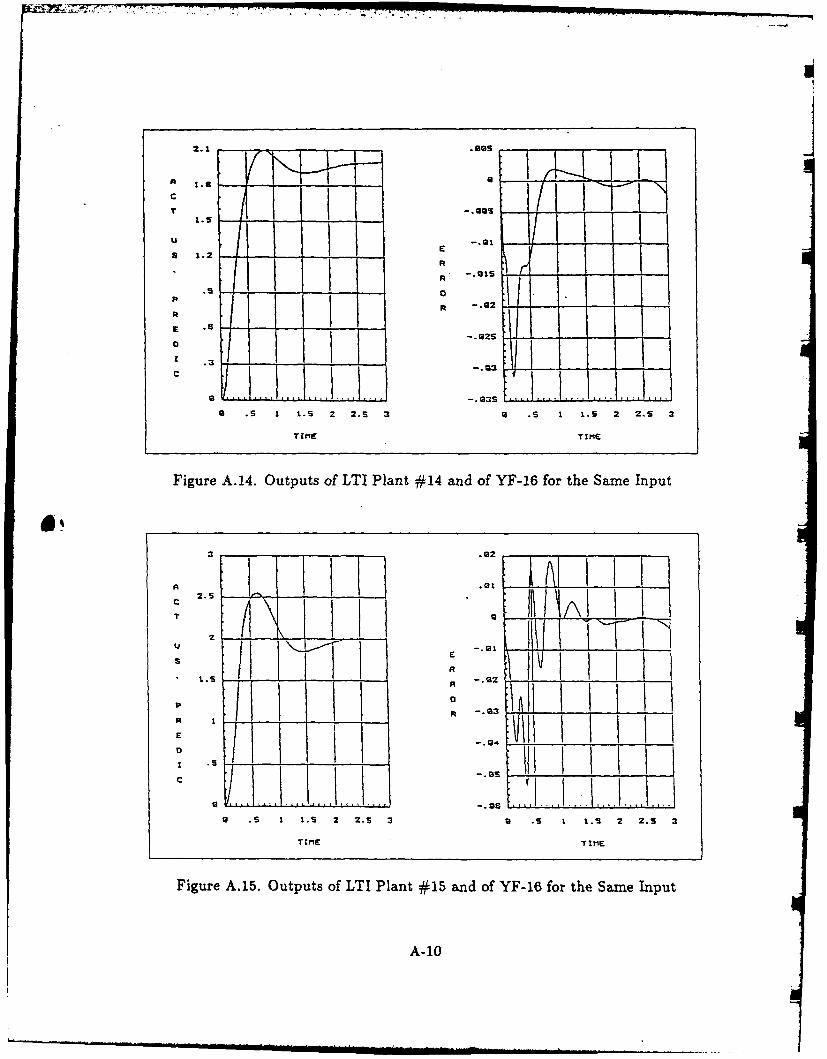
ft I. 1.2
II 0
E _.Qz
E -. 93.
ft 1 T.2~ftT
, -. 035- "
9 .S I .S 2 2.S 3 Q S I 1.S 2 2.S 3
Figure A.14. Outputs of LTI Plant #14 and of YF-16 for the Same Input
A-1
2.5Q
R- IIT
A-0
... . ~ ~ ~ ~ ~ ~ ~ ~ .. .... .' i i li I II I... .I --..... .
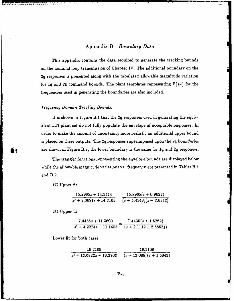
Appendix B. Boundary Data
This appendix contains the data required to generate the tracking bounds
on the nominal loop transmission of Chapter IV. The additional boundary on the
2g responses is presented along with the tabulated allowable magnitude variation
for ig and 2g command bounds. The plant templates representing P(jw) for the
frequencies used in generating the boundaries are also included.
Frequency Domain Tracking Bounds:
It is shown in Figure B.1 that the 2g responses used in generating the equiv-
alent LTI plant set do not fully populate the envelope of acceptable responses. In
order to make the amount of uncertainty more realistic an additional upper bound
is placed on these outputs. The 2g responses superimposed upon the 2g boundaries
are shown in Figure B.2, the lower boundary is the same for 1g and 2g responses.
The transfer functions representing the envelope bounds are displayed below
while the allowable magnitude variations vs. frequency are presented in Tables B.1
and B.2.
1G Upper fit
15.8965s + 14.3414 = 15.8965(s + 0.9022)
s2 + 8.0691s + 14.3165 (s + 5.4349)(s + 2.6342)
2G Upper fit
7.4435s + 11.3600 7.4435(s + 1.5262)S2 + 4.2224s + 11.1403 (s + 2.1112 ± 2.5852j)
Lower fit for both cases
19.2109 19.21092 + 13.6822s + 19.2703 (s + 12.088)(s + 1.5942)
B-1
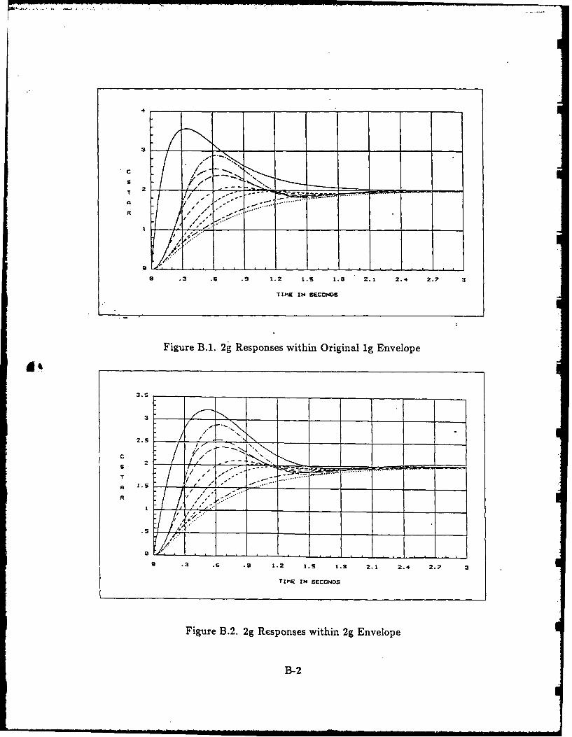
A
0 .3 . .9 1.2 1.S 1.8 2.1 2.4 2.7
TItlE IN SECONDS
Figure B.1. 2g Responses within Original 1g Envelope
C
S
T
R
9 3 .6 .9 1.2 1.9 1.9 2.1 2.4 2.7 3
TIMlE IN SECONDS
Figure B.2. 2g Responses within 2g Envelope
B-2
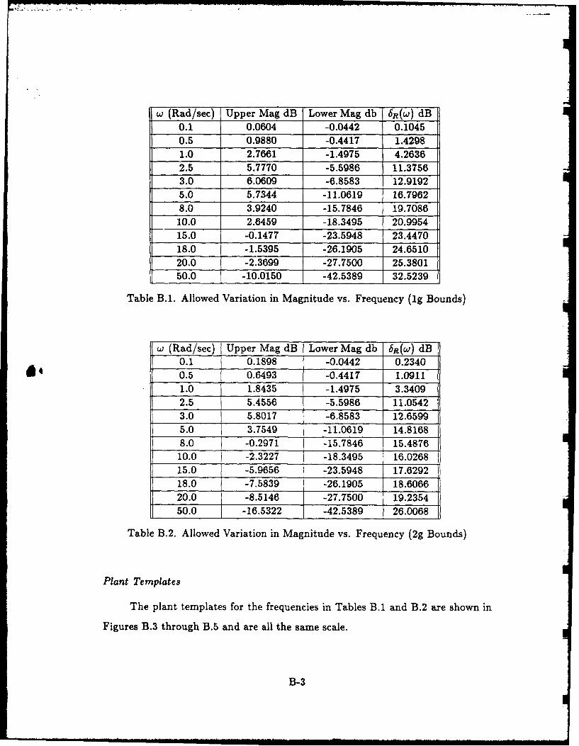
w (Rad/sec) Upper Mag dB Lower Mag db 6 R(w) dB0.1 0.0604 -0.0442 0.10450.5 0.9880 -0.4417 1.42981.0 2.7661 -1.4975 4.26362.5 5.7770 -5.5986 11.37563.0 6.0609 -6.8583 12.91925.0 5.7344 -11.0619 16.79628.0 3.9240 -15.7846 19.708610.0 2.6459 -18.3495 20.995415.0 -0.1477 -23.5948 23.447018.0 -1.5395 -26.1905 24.651020.0 -2.3699 -27.7500 25.380150.0 -10.0150 -42.5389 32.5239
Table B.1. Allowed Variation in Magnitude vs. Frequency (ig Bounds)
w (Rad/sec) Upper Mag dB Lower Mag db bR(w) dB0.1 0.1898 -0.0442 0.2340
4' 0.5 0.6493 -0.4417 1.09111.0 1.8435 -1.4975 3.34092.5 5.4556 -5.5986 11.05423.0 5.8017 -6.8583 12.65995.0 3.7549 -11.0619 14.81688.0 -0.2971 -15.7846 15.487610.0 -2.3227 -18.3495 16.026815.0 -5.9656 -23.5948 17.629218.0 -7.5839 -26.1905 18.606620.0 -8.5146 -27.7500 19.235450.0 -16.5322 -42.5389 26.0068
Table B.2. Allowed Variation in Magnitude vs. Frequency (2g Bounds)
Plant Templates
The plant templates for the frequencies in Tables B.1 and B.2 are shown in
Figures B.3 through B.5 and are all the same scale.
B-3
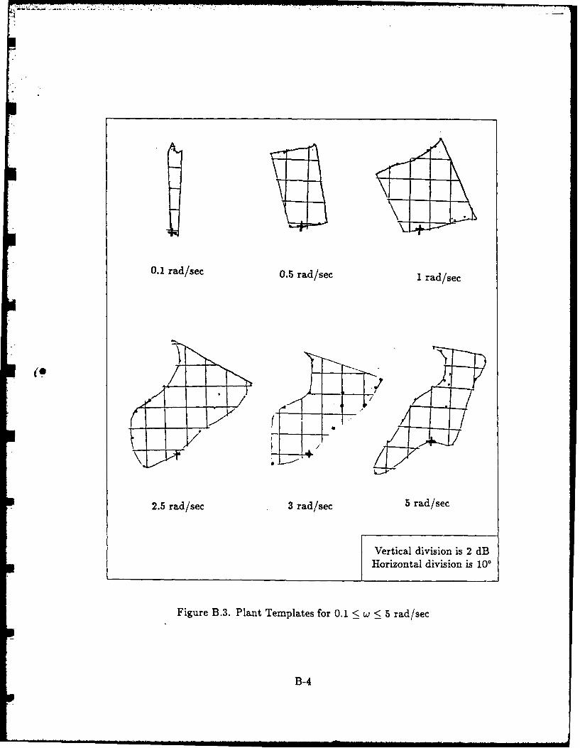
0.1 rad/sec: 0.5 rad/sec 1 rad/sec
(IF
2.5 rad/sec: 3 rad/sec: 5 rad/sec
Vertical division is 2 dBHorizontal division is 100
Figure B.3. Plant Templates for 0.1 <w <- 5 rad/sec
B-4
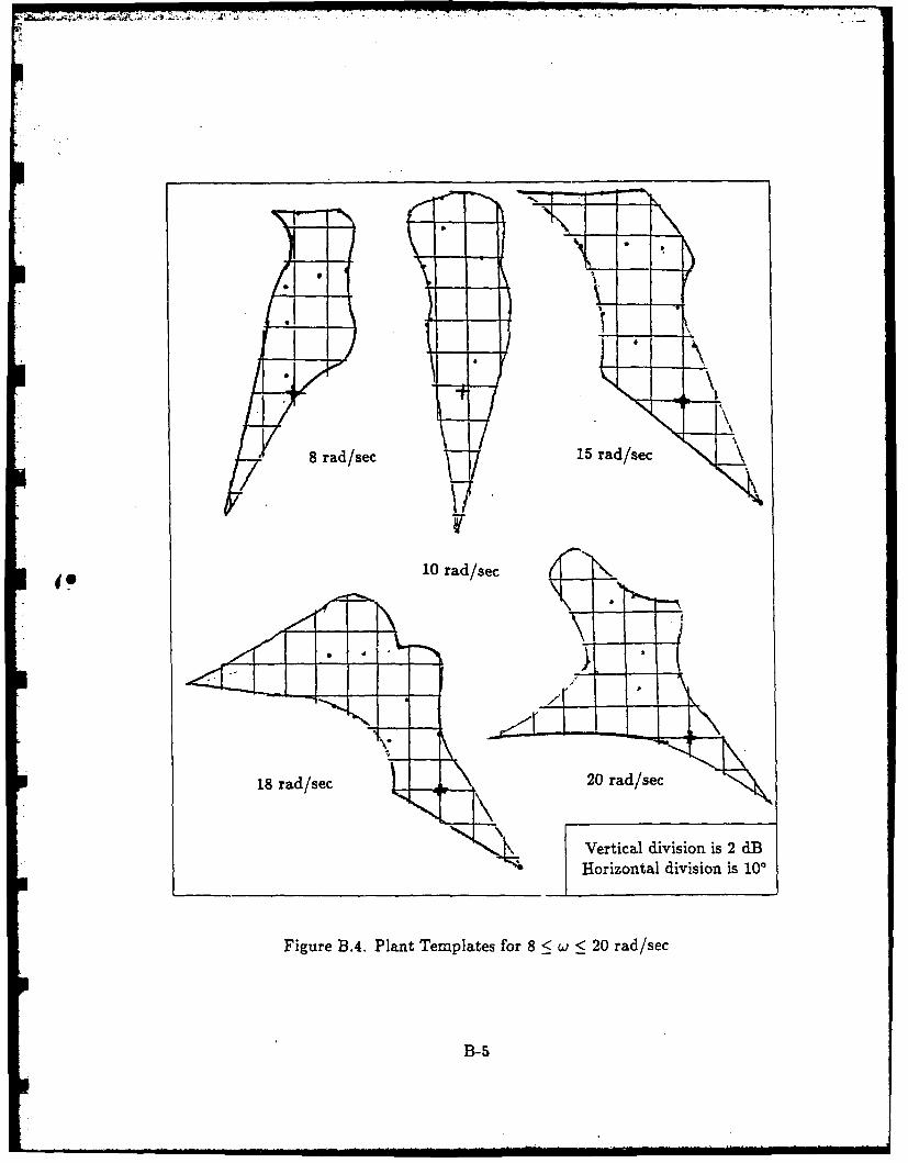
-m 7,
T...8 rad/sec 15 rad/sec:
10 rad/sec
18 rad/sec 20 rad/sec
Vertical division is 2 dB
Horizontal division is 10'
Figure B.4. Plant Templates for 8 < w < 20 rad/sec
B-5
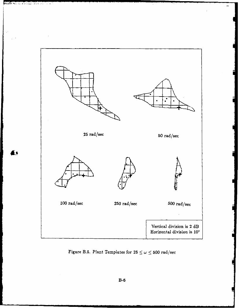
25 rad/sec 50 rad/sec
0 As
100 rad/sec 250 rad/sec 500 rad/sec:
Vertical division is 2 dBHorizontal division is 100
Figure B.5. Plant Templates for 25 <wu < 500 rad/sec
B-6
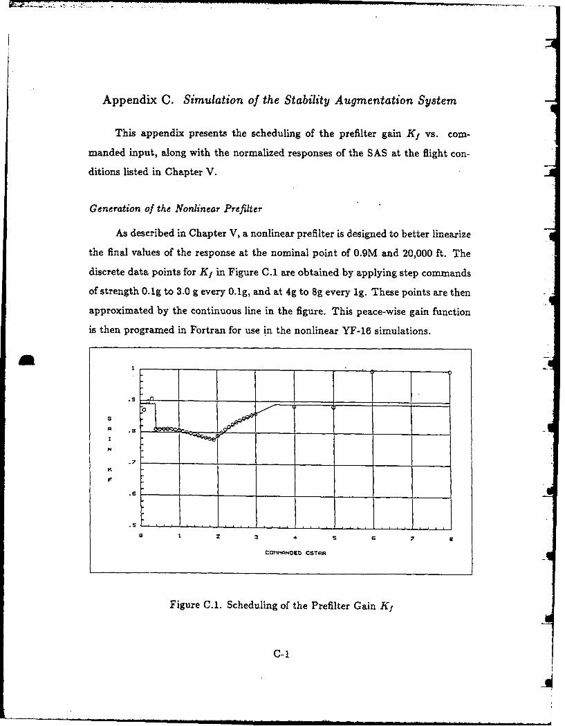
Appendix C. Simulation of the Stability Augmentation System
This appendix presents the scheduling of the prefilter gain K1 vs. com-
manded input, along with the normalized responses of the SAS at the flight con-
ditions listed in Chapter V.
Generation of the Nonlinear Prefilter
As described in Chapter V, a nonlinear prefilter is designed to better linearize
the final values of the response at the nominal point of 0.9M and 20,000 ft. The
discrete data points for K1 in Figure C.1 are obtained by applying step commands
of strength 0.lg to 3.0 g every 0.1g, and at 4g to 8g every 1g. These points are then
approximated by the continuous line in the figure. This peace-wise gain function
is then programed in Fortran for use in the nonlinear YF-16 simulations.
R _ _ --_ _ _G
N
K
.S
COr rANOED CSTAR
Figure C.1. Scheduling of the Prefilter Gain K1
C-1
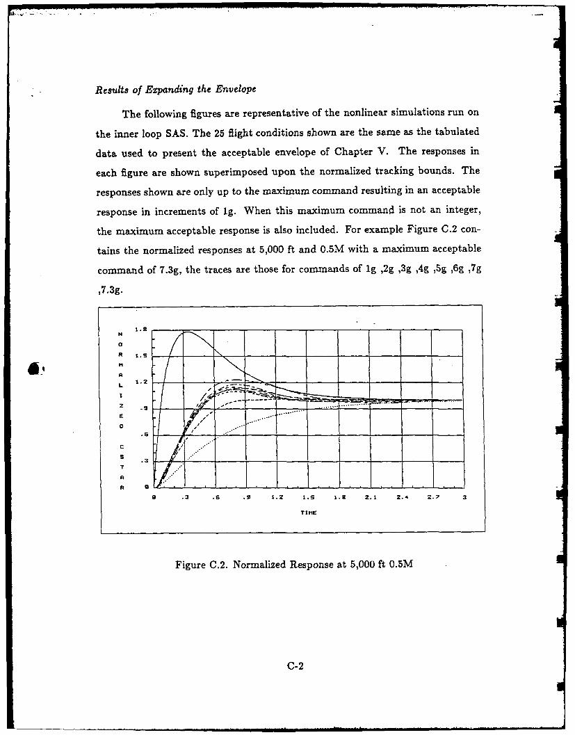
Results of Expanding the Envelope
The following figures are representative of the nonlinear simulations run on
the inner loop SAS. The 25 flight conditions shown are the same as the tabulated
data used to present the acceptable envelope of Chapter V. The responses in
each figure are shown superimposed upon the normalized tracking bounds. The
responses shown are only up to the maximum command resulting in an acceptable
response in increments of 1g. When this maximum command is not an integer,
the maximum acceptable response is also included. For example Figure C.2 con-
tains the normalized responses at 5,000 ft and 0.5M with a maximum acceptable
command of 7.3g, the traces are those for commands of ig ,2g ,3g ,4g ,5g ,6g ,7g
,7.3g.
1-C-
iN
-0- . -- -
R i..,._..-o__
O ..-- ,.A. "
L 1 __...___
R 9
9l .3 .6 .S! 1.2 1.S 1.8 2.1 2.4 2'.?
TIMtE
Figure C.2. Normalized Response at 5,000 ft 0.5M
C-2
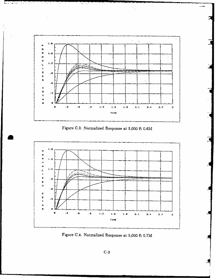
R 1.2 _ _ _ _
L '
2 .......... ____
E
c
S .T
A
a .3 .6 .9 1.2 1.9 1.8 2.1 2.4 2.? 3
TIME
Figure C.3. Normalized Response at 5,000 ft 0.6M
aRM
A
L
2 <,...:-
E
0
A
R 0 V ---......
TI ME
Figure 0.4. Normalized Response at 5,000 ft 0.7M
C-3
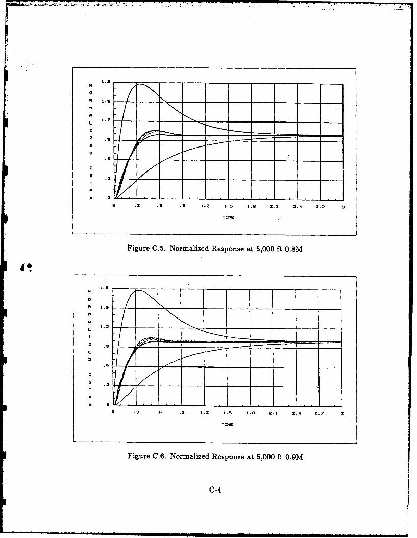
1.2
E
c
a _ _ _ _ _ _
A
9 .3 . .9 1.2 1.5 1.3 2.1 2.4 2.7 3
Figure 0.5. Normalized Response at 5,000 ft 0.8M
2.2 _ _ _ _ _ __ _ _ ___ _ _L
I
2 .9__ ........
.61A
S
A
9 .3 .6 .9 1.2 1.5 1.3 2.1 2.4 2.7 3
Figure 0.6 Normalized Response at 5,000 ft 0.9M
0-4
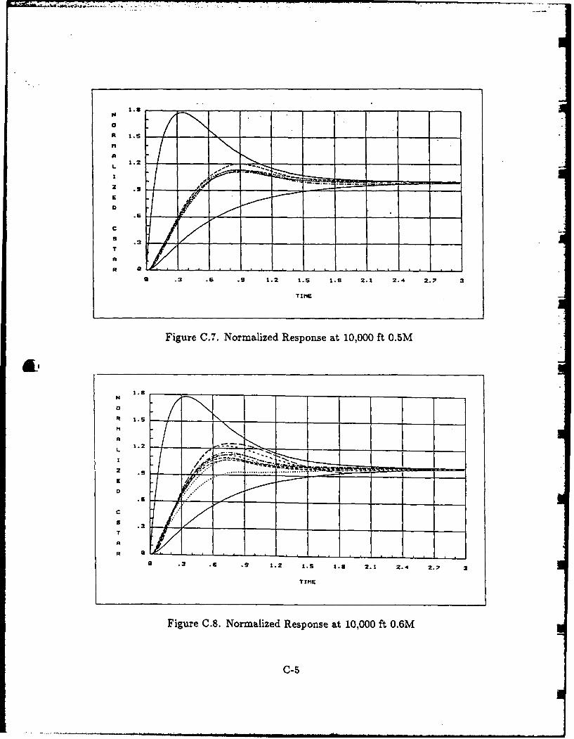
L
S
R
a .3 .6 .9 1.2 I.S 1.8 2.1 2.4 2.7 3
*TIME1
Figure C.7. Normalized Response at 10,000 ft 0.5M
.9.
ft 1.2 _ _ _ _
L
I
2 .
c
S .T
A
* .3 .6 .2 1.2 1.3 1.8 2.1 2.4 2.7 3
TIMlE
Figure 0.8. Normalized Response at 10,000 ft 0.6M
C-5
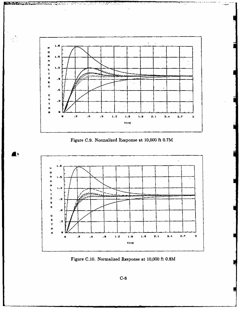
L 1
1; .
A
a .3 .6 .9 1.2 1.S 1.9 2.1 2.4 2.7 3
TIME
Figure C.9. Normalized Response at 10,000 ft 0.7M
A)A
TIM
LL
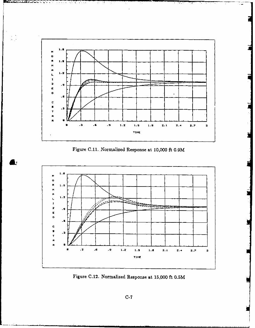
A 1.2
A
R
TIM
R .6
M
9 .3
T
A
U .3 .6 .9 1.2 1.5 1.8 2.1 2.4 2.7 3
TIMlE
Figure C.12. Normalized Response at 10,000 ft 0.5M
aC-7
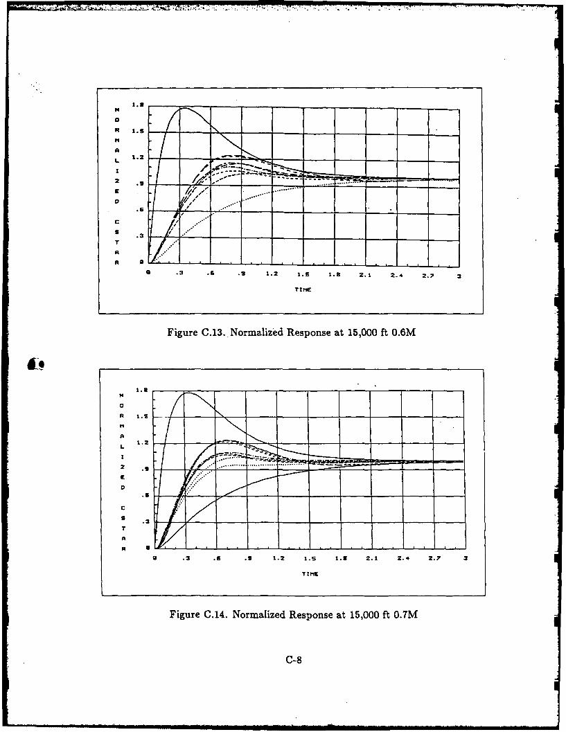
A
L 1.
2
A
R U ~ ~ ---- . 1 - ~ L J4 ~ L .J A
a .3 .6 .S 1.2 1.5 1.3 2.1 2.4 . 3
Figure 0.13..Normalized Response at 15,000 ft 0.6M
R I .
L
9 .3
9 .3 .6 .9 1.2 1.5 1.3 2.1 2.4 2.7 3
TIME
Figure 0.14. Normalized Response at 15,000 ft 0.7M
0-8
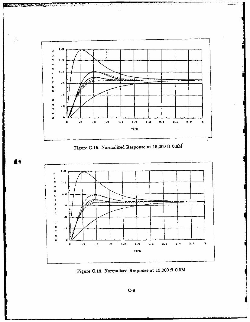
1.2
a
TIm
C-
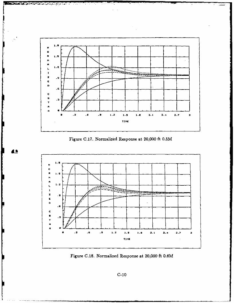
Rrn II
0
TIM
7--
E
D
S .
A
a .3 .6 .9 1.2 1.5 1.8 2.1 2.4 2.7 3
T IE
Figure 0.17. Normalized Response at 20,000 ft 0.5M
C01
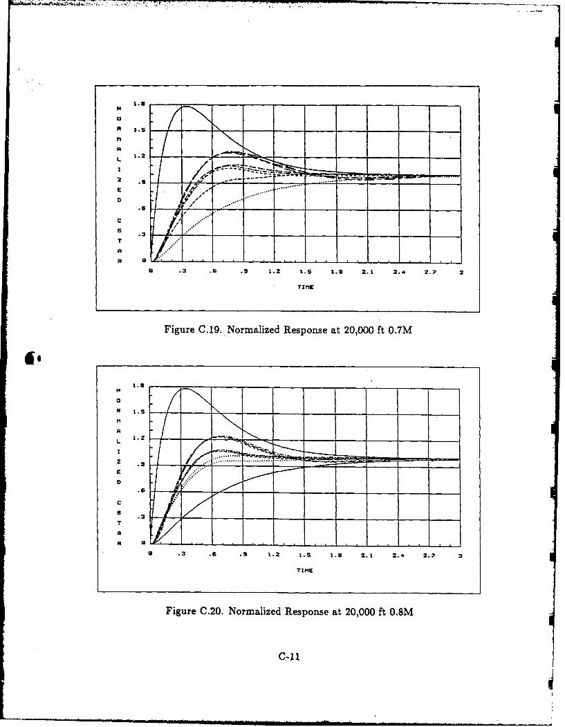
I.
A
L 1.
T .3
A
a .3 .6 .9 1.2 1 S 1.9 2. 1 2.4 2.7 3
Figure C.19.. Normalized Response at 20,000 ft 0.7M
0
Rt____________
II
A
L iI_ _ __ _ _ _ _
I..... ..
S .
a .3 .6 .9 1.2 1.5 1.3 2.1 2.4 2.7 3
TIMlE
Figure C.20. Normalized Response at 20,000 ft 0.8M
C-11
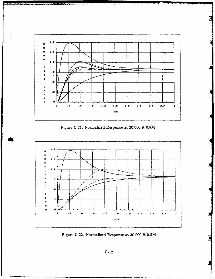
A'1 .
L
2 ___ _ .........
9 .3
A
a .3 .6 .9 1.2 1.9 1.2 2.1 2.4 2.7 3
TIME
Figure 0.21. Normalized Response at 20,000 ft 0.OM
0
M
1 .3T
TIM
C-1
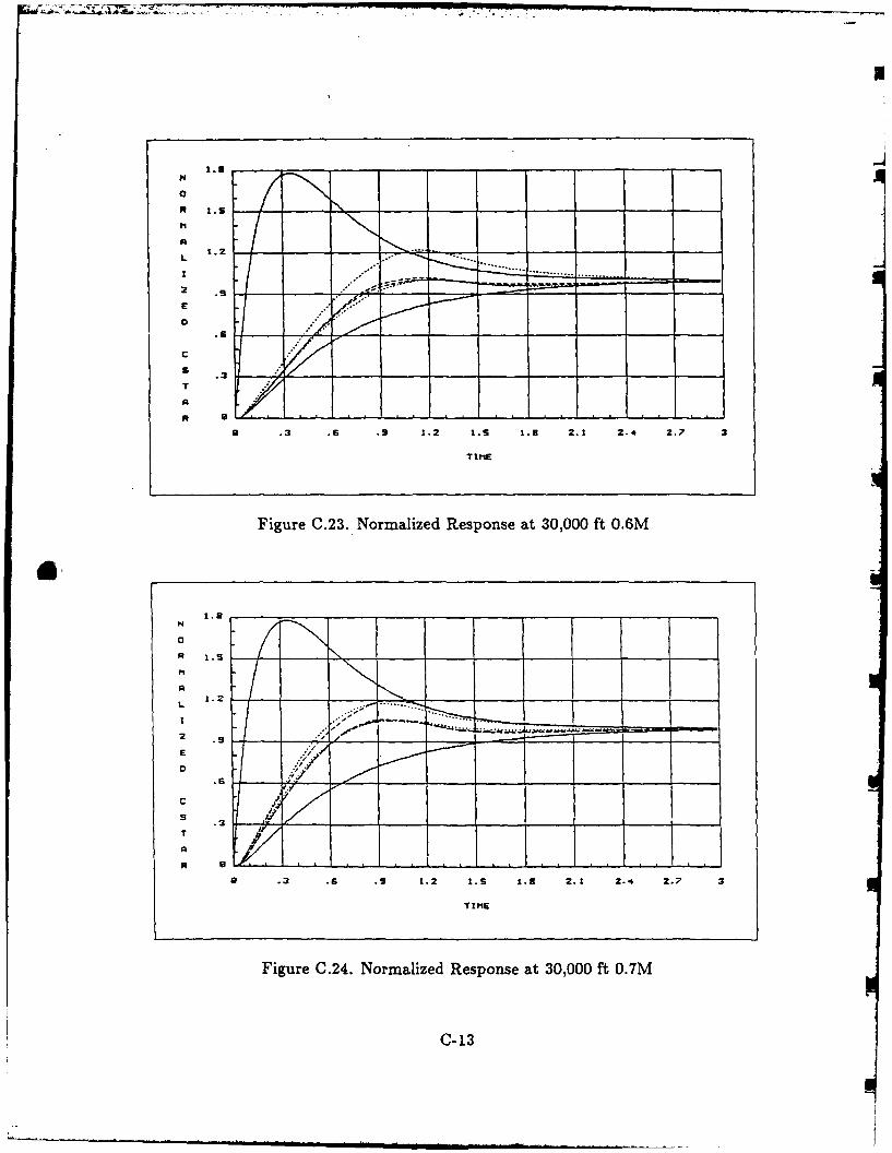
A
.2 . 6 . . . . . .
L
2 .3__ ._1. ____ .1 2 4 .
TIME
Figure 0.23. Normalized Response at 30,000 ft 0.7M
C-1
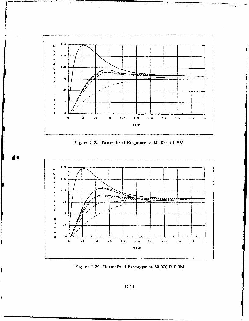
A
L. 1.2.8 2 1 2. .
TI1
S3
a .3 .6 .9 1.2 1.5 1.9 2.1 2.4 2.?
T IME
Figure 0.25. Normalized Response at 30,000 ft 0.9M
Cd1
Appendix D. Fourth Order Pad6 Approximation
The following Pad. method is taken directly from an appendix of a digital
control systems text [11] and applied to the function e" to obtain an approximation
of a pure time delay.
The General Pad Method
The Pad6 method produces rational-fraction approximations of the form
F(x) A,(x) m = 0, 1,2,... (D.1)
for the differentiable power series
d(x) = Co + cIx + cXz2 + C 3 +-. (D.2)
where co 5 0 and F(x) = g(x). Am(x) and Bm(x) are polynomials of the form
Am(x) a0 + aix + a2 x + a3 X3 +-- + amx m (D.3)
Bm(x) = bo + bix + b2 X2 + b3X
3 +." + bmx m (D.4)
where, for this discussion, the coefficients aj and bj are finite values other than
zero.
Let
a0
a,
a= a2 (D.5)
am
bo
b,
b= b2 (D.6)
bm
D-1
C9 Cq-1 ... cq-p
Cp,q- cq1 C9 ."..p+i (D.7)
... ... ... ...
Cq+p-1 Cq+p-2 ... Cq-1
where the elements of Eq (D.1) whose subscripts are negative, that is i - j < 0,
are all zero.
The coefficients of Eqs (D.3) and (D.4) may be solved from the following
matrix equations:
Cm,n+Ib = 0 (D.8)
Cm+i,ob = a (D.9)
The matrices Cm,m+l and Ca+.Io are obtained from Eq (D.7), where for the
former p = m and q = m + I and for the latter p = m + 1 and q = 0. Note that a
and b are (m + 1) x 1 vectors, Cm,,m+i is an m x (m + 1) matrix and Cm+,0 is an
(m + 1) x (m + 1) matrix.
The Approximation
The power series of e2 where x = rs is expanded in a MacLaurin series about
zero, resulting in
X2 X 3 x 4
d(x) = em + x + - + - + - + (D.10)2! 3! 4!
d(x) is to be approximated by the fourth order rational fraction
F (x)= ao + aix + a 2X 2 + a 3X 3 + a 4 X4 (D.11)
bo + blx + b2 x2 + b3 X3 + b4 x
4
where m = 1,c0 c= 1, c2 - ,c 3 - 1, etc. From Eq (D.7) the following are
obtained:
C5 C4 C3 C2 Ci
C 4 ,5 =C 6 CS C4
C3 C2
C7 C6 C5 C4 C3
C 8 C7 C6 C 5 C4
D-2
Lt
Co 0 0 0 0
C1 CO 0 0 0
C5,o= C2 C, CO 0 0
C3 C2 C1 CO 0
C4 C3 C2 C1 CO
Inserting these matrices into Eqs (D.8) and (D.9) results in for Eq (D.8)
1 1 1 15! 24 6 2 b
C,4,b5b = 0 (D.12)1 1 1 1 1I
7! 6! 5! 24 6 bb31 1 1 1 1
8! 7! 6! 5! 24 N
There are only 4 equations and 5 unknowns, setting bo = 1 Eq (D.12) becomes
bo -1,= 5 20 60 120 -1
6 30 120 360b2 = 1 (D.13)
7 42 210 840b3 -1
8 56 336 1680 b4 -1
Solving for b gives
1-1II T
b= -328
-1841
1680
D-3
p
Inserting the values of C,+,o and b into Eq (D.9) results in
1 0 0 0 0 1 ao
1 1 0 0 0 z! a11 00a 1
1 1100 3 -
1 1 1 1 0 -1 a2
6 2 84a 3
1 1 1 1 1 124 6 2 1680
Solving for a gives
28
84
11680
Inserting the values of a, b and x = rs into Eq (D.11) yields,48_ 1680
F(x) = 4 3 - + -1680 e" (D.14)54 -_OS + AOP2 -_0 s + L8
For the pilot model of Chapter VI the time delay of r = -0.3 gives the approxi-
mation used in the nonlinear simulations as
e-0.3a 8 - 66.66753 + 200082 - 3.111 x 10⁴s + 2.0741 x 10s4 + 66.667S3 + 2000S2 + 3.111 x 10⁴s + 2.0741 x 10⁵
(s - 14.03 ± j17.7)(s - 19.31 ± j5.78)
(s + 14.03 ± j17.7)(s + 19.31 ± j5.78) (D15)
D-4
Bibliography
1. Barfield, Finley Head Control Engineer AFTI/F-16. Personal interviews.Flight Dynamics Labs, Wright-Patterson AFB, OH 28 January through De-cember 1988.
2. Dameron, Capt Gary G. A Real-Time Simulator for Man-in-the-Loop Testingof Aircraft Control Systems (SIMTA CS-RT). MS thesis, AFIT/GE/ENG/88D-8. School of Engineering, Wright-Patterson AFB OH, December 1988.
3. D'Azzo, John J. Unpublished lecture notes from EENG 640, Automatic Con-trol I. School of Engineering, Air Force Institute of Technology, Wright-Patterson AFB OH, Winter 1988.
4. East, D. J. "A New Approach to Optimal Loop Synthesis," International Jour-nal of Control, 54: 731-748 (1981).
5. Hamilton, 2Lt Steve W. QFT Digital Controller for an Unmanned Re-search Vehicle with an Improved Method for Choosing the Control Weightings.MS thesis, AFIT/GE/ENG/87D-22. School of Engineering, Wright-PattersonAFB OH, December 1987.
6. Horowitz, Isaac M. "Improvement in Quantitative Nonlinear Feedback Designby Cancellation," International Journal of Control, 94: 547-560 (1981).
7. Horowitz, Isaac M. and Moshe Breiner. "Quantitative Synthesis of FeedbackSystems with Uncertain Nonlinear Multivariable Plants," International Jour-nal of Systems Science, 12: 539-563 (1981).
8. Horowitz, Isaac M. et al. Research in Advanced Flight Control Design, 1 June1977 - 31 May 1979. Contract AFOSR-77-3355. Rehovot Israel: Dept of Ap-plied Mathematics The Weizmann Institute of Science, January 1980 (AD-A082424).
9. Horowitz. Isaac M. and Uri Shaked. "Superiority of Transfer Function OverState-Variable Methods in Linear Time-Invariant Feedback System Design,"IEEE Transactions on Automatic Control, 20: 84-97 (February 1975).
10. Horowitz, Isaac M. "Synthesis of Feedback Systems with Nonlinear Time-Varying Uncertain Plants to Satisfy Quantitative Performance Specifica-tions, " Proceedings of the IEEE, 64: 123-130 (January 1976).
11. Horowitz, Isaac M. "The Singular-G Method for Unstable Non-Minimum-Phase Plants," International Journal of Control, 49: 533-541 (1986).
12. Houpis, Constantine H. and Gary B. Lamont. Digital Control Systems Theory,Hardware, Software. New York: McGraw Hill Book Company, 1988.
13. Houpis, Constantine H. Quantitative Feedback Theory, AFWAL-TR-86-3107.Dayton OH: AFWAL/FIGL, January 1987.
BIB-1
14. Houpis, Constantine H. Unpublished lecture notes from EENG 743, LiteratureStudy in Current Control Topics. School of Engineering, Air Force Instituteof Technology, Wright-Patterson AFB OH, Winter 1988.
15. Kabrisky, Matthew. Unpublished lecture notes from EENG 548, Human Fac-tors Engineering. School of Engineering, Air Force Institute of Technology,Wright-Patterson AFB OH, Fall 1988.
16. Kassan, 2Lt Mark W. F-16 Simulator for Man-in-the-Loop Testing of AircraftControl Systems (SIMTACS). MS thesis, AFIT/GE/ENG/87D-30. School ofEngineering, Wright-Patterson AFB OH, December 1987.
17. Krishnan, K. R. and A. Cruickshanks. "Frequency-domain Design of FeedbackSystems for Specified Insensitivity of Time-domain Response to ParametricVariation," International Journal of Control, 25: 609-620 (1977).
18. Neal, T. Peter, and Rogers E. Smith. An In-Flight Investigation to DevelopControl System Design Criteria for Fighter Airplanes, AFFDL-TR-70-74, Vol.I, Air Force Flight Dynamics Laboratory: Wright-Patterson AFB Ohio, De-cember 1970.
19. Quinlivan, Richard P. Multimode Flight Control Definition Study: Final Re-port, 29 March 1971 - 29 March 1972. Contract F33615-71-C-1485. Bingham-ton NY: G.E. Aerospace Instruments and Control System Department, May1972.
20. Tobie, H. N., E. M. Elliott, and L.G. Malcom. A New Longitudinal HandlingQualities Criterion, National Aerospace Electronics Conference, Dayton Ohio,16-18 May 1966.
21. Yaniv, 0., Department of Electrical Engineering, Tel Aviv University. Personalinterview. AFIT School of Engineering, Dayton OH, December 1987.
BIB-2
Vita
Lieutenant Thomas J. Kobylarz was born on
He graduated from high school in Ewing Twp., New Jersey in 1981 and
attended the United States Air Force Academy from which he received the degree
of Bachelor of Science in Electrical Engineering in May 1986, Upon graduation he
received a regular commission in the Air Force and attended undergraduate pilot
training at Laughlin AFB Texas from July 1986 to May 1987. In June o 1987 he
entered the School of Engineering, 'ir Force Institute of Technology studying for
a Masters Degree in Electrical Engineering.
Lieutenant Kobylarz is a member of the Tau Beta Pi and Eta Kappa Nu
honor societies. Following his graduation fror. AFIT he will be assigned to the
4 9 5 0 b Test Wing, WPAFB Ohio.
VITA-1
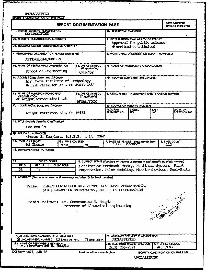
SECURITY CLASSIFICATION OF THIS PAGE
IFor", ApprovedREPORT DOCUMENTATION PAGE OMBNo. 0704-0188
/ REPORT SECURITY CLASSIFICATION lb. RESTRICTIVE MARKINGSL14CLASSIFIED
2a. SECURITY CLASSIFICATION AUTHORITY 3. DISTRIBUTION /AVAILABIUTY OF REPORTApproved for public release;
2b. DECLASSIFICATION I DOWNGRADING SCHEDULE distribution unlimited
4. PERFORMING ORGANIZATION REPORT NUMBER(S) S. MONITORING ORGANIZATION REPORT NUMBER(S)
AFIT/GE/ENG/88D-19
6a. NAME OF PERFORMING ORGANIZATION 6b. OFFICE SYMBOL 7a. NAME OF MONITORING ORGANIZATIONSchol ofEngieerigif appikabeJ
School of E AFIT/ENG
6r. ADDRESS (CIy, State, and ZIPCode) 7b. ADDRESS (City. State, and ZIP Code)
Air Force Institute of TechnologyWright-Patterson AFB, OH 45433-6583
a. NAME OF FUNDING/SPONSORING Sb. OFFICE SYMBOL 9. PROCUREMENT INSTRUMENT IDENTIFICATION NUMBERORGA?4IZATION (If applicable)
AF Wrht.LAronautical Jzb
ADDRESS (City, State, and ZIP Code) 10. SOURCE OF FUNDING NUMBERSPROGRAM PROJECT TASK IWORK UNIT
Wright-Patterson AFB, OH 45433 ELEMENT NO. NO. NOrCCESSION NO.
/
11. TITLE (include Security Classification)
See box 19
. PERSONAL AUTHOR(S)Thcmas J. Kobylarz, B.S.E.E. 1 Lt, USAF
13a. TYPE OF REPORT 113b. TIME COVERED 114. OFp REEORT (YoarMorrth, Day) 115. PAGE COUNTMS Thesis FROM TO___ 1988 J~~ 113
16. SUPPLEMENTARY NOTATION
17. COSATI CODES 18. SUBJECT TERMS (Continue on reverse if necessary and identify by block number)
FIELD GROUP I SUB-GROUP Quantitative Feedback Theory, Nonlinear Systems, Pilot01 04- Compensation, Pilot Modeling, Man-in-the-loop, Neal-SmithI I
19. ABSTRACT (Continue on reverse if necessary and identify by block number)
Title: FLIGHT CNt1'WLLER DESIGN WITH NCKLINEAR AERCDYNAMICS,LARGE PAPAMETER UN AJN'TY, AND PILOT CCIENSATION
Thesis Chairman: Dr. Constantine H. Houpis .Professor of Electrical Engineering
vs
'..ISTRIBUTION I AVAILABIUTY OF ABSTRACT 21. ABSTRACT SECURITY CLASSIFICATION
I %glUNCLASSIFIEDAJNLIMITED 3 SAME AS RPT. [ DTIC USERS UN4CLASSIFIEDI 22a. AME OF RESPONSJBLE INDIV DUAL. 22b. TELEPHONE (Include Area Code) 22c. OFFICE SYMBOL
Dr. Constant = is (513) 255-2024 1 AFIT/ENG
DO Form 1473, JUN 86 Previous editions are obsolete. SECURITY CLASSIFICATION OF THIS PAGE
UNCLASSIFIED
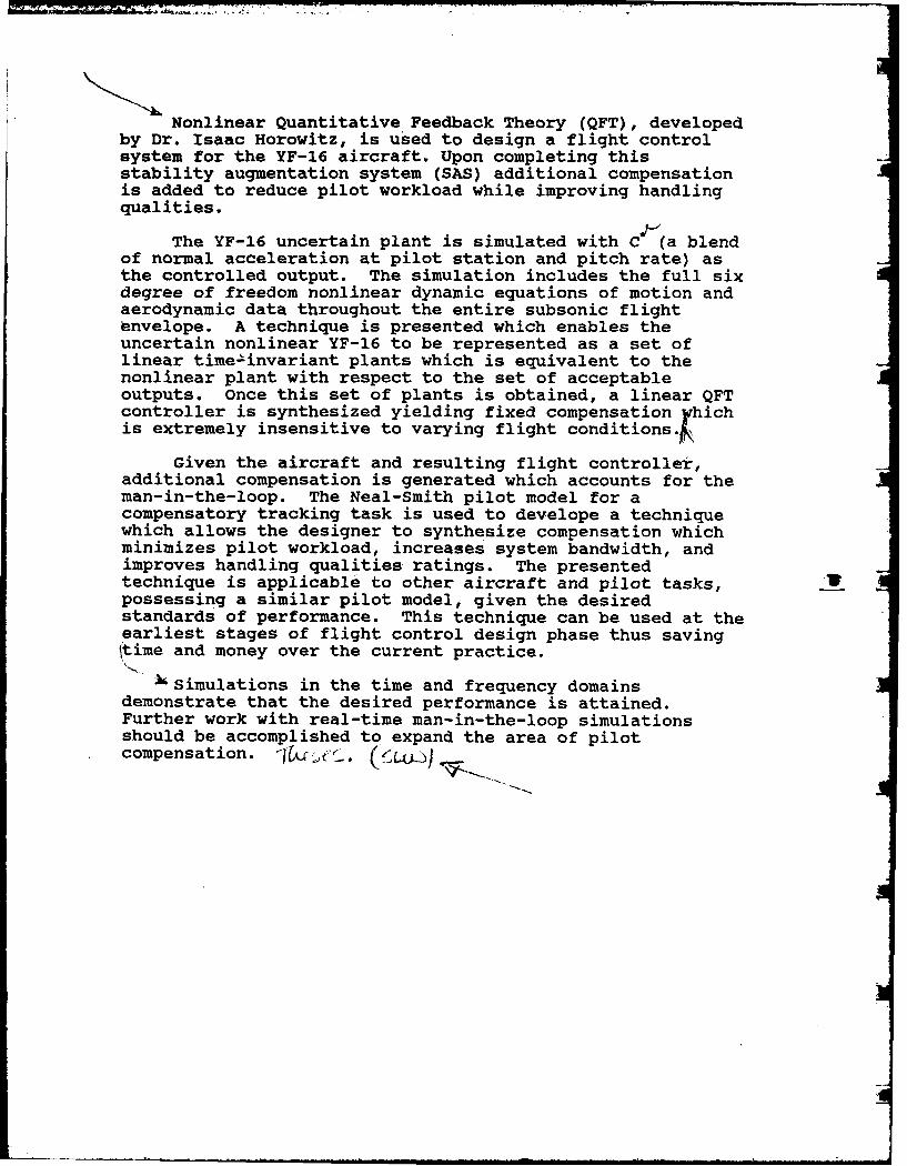
Nonlinear Quantitative Feedback Theory (QFT), developedby Dr. Isaac Horowitz, is used to design a flight controlsystem for the YF-16 aircraft. Upon completing thisstability augmentation system (SAS) additional compensationis added to reduce pilot workload while improving handlingqualities.
The YF-16 uncertain plant is simulated with C (a blendof normal acceleration at pilot station and pitch rate) asthe controlled output. The simulation includes the full sixdegree of freedom nonlinear dynamic equations of motion andaerodynamic data throughout the entire subsonic flightenvelope. A technique is presented which enables theuncertain nonlinear YF-16 to be represented as a set oflinear time-invariant plants which is equivalent to thenonlinear plant with respect to the set of acceptableoutputs. Once this set of plants is obtained, a linear QFTcontroller is synthesized yielding fixed compensation .hichis extremely insensitive to varying flight conditions.
Given the aircraft and resulting flight controller,additional compensation is generated which accounts for theman-in-the-loop. The Neal-Smith pilot model for acompensatory tracking task is used to develope a techniquewhich allows the designer to synthesize compensation whichminimizes pilot workload, increases system bandwidth, andimproves handling qualities ratings. The presentedtechnique is applicable to other aircraft and pilot tasks,possessing a similar pilot model, given the desiredstandards of performance. This technique can be used at theearliest stages of flight control design phase thus saving(time and money over the current practice.
,1 Simulations in the time and frequency domainsdemonstrate that the desired performance is attained.Further work with real-time man-in-the-loop simulationsshould be accomplished to expand the area of pilotcompensation. i(x 0 (t .