Embed Size (px)
Citation preview

Noise Estimation from a Single Image
Ce Liu William T. Freeman
CS and AI Lab, MIT
celiu,[email protected]
Richard Szeliski Sing Bing Kang
Microsoft Research
szeliski,[email protected]
Abstract
In order to work well, many computer vision algorithms
require that their parameters be adjusted according to the
image noise level, making it an important quantity to es-
timate. We show how to estimate an upper bound on the
noise level from a single image based on a piecewise smooth
image prior model and measured CCD camera response
functions. We also learn the space of noise level functions–
how noise level changes with respect to brightness–and use
Bayesian MAP inference to infer the noise level function
from a single image. We illustrate the utility of this noise
estimation for two algorithms: edge detection and feature-
preserving smoothing through bilateral filtering. For a vari-
ety of different noise levels, we obtain good results for both
these algorithms with no user-specified inputs.
1. Introduction
Many computer vision algorithms can work well only
if the parameters of the algorithm are hand-tweaked to
account for characteristics of the particular images under
study. One of the most common needs for algorithm pa-
rameter adjustment is to account for variations in noise
level over input images. These variations can be caused
by changes in the light level or acquisition modality, and
the amount of variation can be severe. An essential step
toward achieving reliable, automatic computer vision algo-
rithms is the ability to accurately estimate the noise level of
images. Examples of algorithms requiring noise level es-
timates include motion estimation [1], denoising [12, 11],
super-resolution [5], shape-from-shading [19], and feature
extraction [9].
Estimating the noise level from a single image seems like
an impossible task: we need to recognize whether local im-
age variations are due to color, texture, or lighting variations
from the image itself, or due to the noise. It might seem that
accurate estimation of the noise level would require a very
sophisticated prior model for images. However, in this work
we use a very simple image model–piecewise smooth over
segmented regions–to derive a bound on the image noise
level. We fit the image data in each region with a smooth
function and estimate the noise using the residual. Such es-
timates are guaranteed to be over-estimates of the true noise
variance, since the regions can contain image variations that
are not being modeled. However, there are usually some re-
gions in each image for which the simple model holds, and
we find that our noise bounds are usually tight. While we
assume that auxiliary camera information is unknown, the
algorithm proposed in this paper can easily be augmented
with such information.
Unfortunately, real CCD camera noise is not simply ad-
ditive; it is strongly dependent on the image intensity level.
We call the noise level as a function of image intensity the
noise level function, or NLF. Since it may not be possible
to find image regions at all the desired levels of intensity or
color needed to describe the noise level function, we use the
Columbia camera response function database [6] to model
the NLF using principal components and bounds on deriva-
tives. These principal components serve as a prior model to
estimate the NLF over regions of missing data. We use a
Bayesian MAP framework to estimate the noise level func-
tions in RGB channels, using the bounds derived from the
noise estimates over each image region. Experiments on
both synthetic and real data demonstrate that the proposed
algorithm can reliably infer noise levels.
To illustrate that estimating the noise can make vision
algorithms more robust, we apply our noise inference to
two algorithms: bilateral filtering for feature-preserving
smoothing, and edge detection. The resulting algorithms,
properly accounting for image noise, show robust behavior
over a wide range of noise conditions.
The paper is organized as follows. We review related
work in Sect. 2. In Sect. 3, we describe our camera noise
model and show how it can be combined with a set of pa-
rameterized camera response functions to develop a prior on
the noise response function. We show how to estimate the
noise level function in Sect. 4 using a combination of per-
region variance estimation and the prior model on NLFs.
We provide experimental results in Sect. 5 and apply those
estimates to the two computer vision algorithms in Sect. 6.
We conclude in Sect. 7.

Atmospheric
Attenuation
Lens/geometric
Distortion
CCD Imaging/
Bayer Pattern
Fixed Pattern
Noise
Shot Noise
Thermal
Noise
Interpolation/
DemosaicWhite
Balancing
Gamma
CorrectionA/D Converter
Dark Current
Noise
t
Quantization
Noise
Scene
Radiance
Digital
Image
Figure 1. CCD camera imaging pipeline, redrawn from [18].
2. Related Work
There is a large literature on image denoising. Although
very promising denoising results have been achieved using a
variety of methods, such as wavelets [12], anisotropic diffu-
sion [11] and bilateral filtering [17], the noise level is often
assumed known and constant for varying brightness values.
In contrast, the literature on noise estimation is very lim-
ited. Noise can be estimated from multiple images or a
single image. Estimation from multiple image is an over-
constrained problem, and was addressed in [7]. Estimation
from a single image, however, is an under-constrained prob-
lem and further assumptions have to be made for the noise.
In the image denoising literature, noise is often assumed
to be additive white Gaussian noise (AWGN). A widely
used estimation method is based on mean absolute devia-
tion (MAD) [3]. In [15], the authors proposed three meth-
ods to estimate noise level based on training samples and
the statistics (Laplacian) of natural images. However, real
CCD camera noise is intensity-dependent.
3. Noise Study
In this section, we build a model for the noise level func-
tions of CCD cameras. In Subsect. 3.1 we introduce the
terms of our camera noise model, showing the dependence
of the noise level function (the noise variance as function
of brightness) on the camera response function (the image
brightness as function of scene irradiance). Given a cam-
era response function, described in Subsect. 3.2, we can
synthesize realistic camera noise, as shown in Subsect. 3.3.
Thus, in Subsect. 3.4, from a parameterized set of camera
response functions (CRFs), we derive the set of possible
noise level functions. This restricted class of NLFs allows
us to accurately estimate the NLF from a single image, as
described in Sect. 4.
3.1. Noise Model of CCD Camera
The CCD digital camera converts the irradiance, the pho-
tons coming into the imaging sensor, to electrons and finally
to bits. See Figure 1 for the imaging pipeline of CCD cam-
era. There are mainly five noise sources as stated in [7],
namely fixed pattern noise, dark current noise, shot noise,
amplifier noise and quantization noise. These noise terms
are simplified in [18]. Following the imaging equation in
[18], we propose the following noise model of a CCD cam-
era
I = f(L + ns + nc) + nq, (1)
where I is the observed image brightness, f(·) is camera re-
sponse function (CRF), ns accounts for all the noise compo-
nents that are dependent on irradiance L, nc accounts for the
independent noise before gamma correction, and n q is addi-
tional quantization and amplification noise. Since nq is the
minimum noise attached to the camera and most cameras
can achieve very low noise, nq will be ignored in our model.
We assume noise statistics E(ns) = 0, Var(ns) = Lσ2s and
E(nc) = 0, Var(nc) = σ2c . Note the linear dependence of
the variance of ns on the irradiance L [18].
3.2. Camera Response Function (CRF)
The camera response function models the nonlinear pro-
cesses in a CCD camera that perform tonescale (gamma)
and white balance correction [14]. There are many
ways to estimate camera response functions given a set
of images taken under different exposures. To ex-
plore the common properties of many different CRFs,
we downloaded 201 real-world response functions from
http://www.cs.columbia.edu/CAVE [6]. Note that we
only chose 190 saturated CRFs since the unsaturated curves
are mostly synthesized. Each CRF is a 1024-dimensional
vector that represents the discretized [0, 1]→ [0, 1] function,
where both irradiance L and brightness I are normalized to
be in the range [0, 1]. We use notation crf(i) to represent the
ith function in the database.
3.3. Synthetic CCD Noise
In principle, we could set up optical experiments to mea-
sure precisely for each camera how the noise level changes
with image brightness. However, this would be time con-
suming and might still not adequately sample the space of
camera response functions. Instead, we use numerical sim-
ulation to estimate the noise function. The basic idea is to
transform the image I by the inverse camera response func-
tion f−1 to obtain an irradiance plane L. We then take L
through the processing blocks in Figure 1 to obtain the noisy
image IN .
A direct way from Eqn. (1) is to reverse transform I
to irradiance L, add noise independently to each pixel, and
transform to brightness to obtain IN . This process is shown
in Figure 2 (a). The synthesized noise image, for the test
pattern (c), is shown in Figure (d).
Real CCD noise is not white, however; there are spatial
correlations introduced by “demosaicing” [13], i.e., the re-
I IN
n cn s
crf
0 0.5 10
0.2
0.4
0.6
0.8
1
Irradiance
Bri
gh
tne
ss
crf
0 0.5 10
0.2
0.4
0.6
0.8
1
Irradiance
Bri
gh
tne
ss
crf
0 0.5 10
0.2
0.4
0.6
0.8
1
Irradiance
Bri
gh
tne
ss
0 0.5 10
0.2
0.4
0.6
0.8
1
Irra
dia
nc
eBrightness
icrf
0 0.5 10
0.2
0.4
0.6
0.8
1
Irra
dia
nc
e
Brightness
icrfI IN
n cn s
Bayer Pattern
& Demosaic
Bayer Pattern
& Demosaic
(a) White (independent) CCD noise synthesis
(b) Correlated CCD noise synthesis by going through Bayer pattern
L
L
(c) (d) (e) (f) (g)
Figure 2. Block diagrams showing noise simulations for color
camera images. (a) shows independent white noise synthesis; (b)
adds CCD color filter pattern sensing and demosaicing to model
spatial correlations in the camera noise [8]. (c): test pattern. (d)
and (e): the synthesized images of (a) and (b). (f) and (g): the
corresponding autocorrelation.
construction of three colors at every pixel from the single-
color samples measured under the color filter array of the
CCD. We simulate this effect for a common color filter
pattern (Bayer) and demosaicing algorithm (gradient-based
interpolation [8]); we expect that other filter patterns and
demosaicing algorithms will give comparable noise spatial
correlations. We synthesized CCD camera noise in accor-
dance with 2 (b) and took the difference between the de-
mosaiced images with and without noise, adding that to the
original image to synthesize CCD noise. The synthesized
noise is shown in Figure 2 (e). The autocorrelation func-
tions for noise images (d) and (e) are shown in (f) and (g),
respectively, showing that the simulated CCD noise shows
spatial correlations after taking into account the effects of
demosaicing.
3.4. The Space of Noise Level Functions
We define the noise level function (NLF) as the varia-
tion of the standard deviation of noise with respect to image
intensity. This function can be computed as
τ(I) =√
E[(IN − I)2], (2)
where IN is the observation and I = E(IN ). Essentially
this is a function of how standard deviation changes with
respect to the mean value.
0 0.2 0.4 0.6 0.8 10
0.2
0.4
0.6
0.8
1
Irradiance
Bri
gh
tnes
s
0 0.2 0.4 0.6 0.8 10
5
10
15
20
Irradiance
Der
ivat
ive
of
Bri
gh
tnes
s
0 0.2 0.4 0.6 0.8 10
0.02
0.04
0.06
0.08
0.1
Brightness
Sta
nd
ard
Dev
iati
on
(a) CRFs (b) Derivative of CRFs (c) NLF
Figure 3. The blue and red curves correspond to crf(50) and
crf(60). The NLFs are estimated at σs =0.06, σc =0.02.
Based on the CCD camera noise model Eqn. (1) and
noise synthesis process, IN is a random variable dependent
on the camera response function f and noise parameters σ s
and σc. Because L = f−1(I), the noise level function can
also be written as
τ(I; f, σs, σc) =√
E[(IN (f−1(I), f, σs, σc) − I)2], (3)
where IN (·) is the noise synthesis process.
We use numerical simulation to estimate the noise func-
tion given f , σs and σc, for each of red, green and blue
channels. The smoothly changing pattern in Figure 2 (c) is
used to estimate Eqn. (3). To reduce statistical fluctuations,
we use an image of dimension 1024× 1024 and take the
mean of 20 samples for each estimate.
To see how the noise function changes with respect to
parameter f , we examine two CRFs, crf(50) and crf(60),
as shown in Figure 3 (a). Their derivatives are plotted in
(b). The corresponding NLFs, which have been computed
at σs = 0.06, σc = 0.02, are plotted in (c). Notice that the
derivative of crf(50) is significant at zero irradiance, result-
ing in high noise standard deviation there. It is clear that
the NLFs are highly dependent on the derivative function.
To represent the whole space of noise level functions, we
draw samples of τ(·; f, σs, σc) from the space of f , σs and
σc. The downloaded 190 CRFs are used to represent the
space of f . We found that σs = 0.16 and σc = 0.06 result
in very high noise, so these two values are set as the max-
imum of the two parameters. We sample σs from 0.00 to
0.16 with step size 0.02, and sample σc from 0.01 to 0.06with step size 0.01. We get a dense set of samples τiK
i=1
of NLFs, where K =190×9×6=10, 260. Using principal
component analysis (PCA), we get mean noise level func-
tion τ , eigenvectors wimi=1 and the corresponding eigen-
values υimi=1. Thus, a noise function can be represented
as
τ = τ +
m∑
i=1
βiwi, (4)
where coefficient βi is Gaussian distributed βi ∼ N (0, υi),and the function must be positive everywhere, i.e.,
τ +
m∑
i=1
βiwi 0, (5)
0 0.2 0.4 0.6 0.8 10.01
0.02
0.03
0.04
0.05
0.06
0.07
0.08
0.09
0.1
Brightness
No
ise
Lev
el
0 0.2 0.4 0.6 0.8 1−0.2
−0.15
−0.1
−0.05
0
0.05
0.1
0.15
0.2
Brightness
Nois
e L
evel
1st eigenvector2nd eigenvector3rd eigenvector4th eigenvector5th eigenvector6th eigenvector
(a) Mean of noise functions (b) Eigenvectors of noise functions
0 0.2 0.4 0.6 0.8 1−5
0
5
Brightness
1st
−O
rder
Der
ivat
ive
of
No
ise
Lev
el
upper bound of 1st order derivativelower bound of 1st order derivativefeasible area of 1st order derivative
0 0.2 0.4 0.6 0.8 1−200
−150
−100
−50
0
50
100
150
Brightness
2nd−
Ord
er D
eriv
ativ
e of
Nois
e L
evel
upper bound of 2nd order derivativelower bound of 2nd order derivativefeasible area of 2nd order derivative
(c) The bounds of 1st-order derivatives (d) The bounds of 2nd-order derivatives
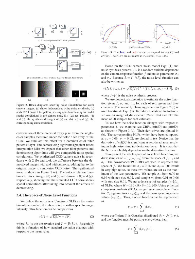
Figure 4. Camera noise function properties.
where τ, wi ∈ Rd and d = 256. This inequality constraint
implies that noise functions lie inside a cone in β space.
The mean noise function and eigenvectors are displayed in
Figure 4 (a) and (b), respectively.
Eigenvectors serve as basis functions to impose smooth-
ness to the function. We also impose upper and lower
bounds on 1st and 2nd order derivatives to further constrain
noise functions. Let T ∈ R(d−1)×d and K ∈ R
(d−2)×d be
the matrix of 1st- and 2nd-order derivatives [16]. The con-
straints can be represented as
bmin Tτ bmax, hmin Kτ hmax, (6)
where bmin, bmax ∈ Rd−1, hmin, hmax ∈ R
d−2 are esti-
mated from the training data set τiKi=1.
4. Noise Estimation from a Single Color Image
Noise estimation and image denoising are in general
chicken and egg problems. To estimate the noise level, the
underlying signal must be known, which could be estimated
using a denoising algorithm; conversely, most denoising al-
gorithms depend on knowing the noise level. Sophisticated
algorithms such as EM might find a stationary point, but al-
gorithms including denoising as an inner loop might be too
slow to be practical. Instead, we propose a rough estimate
of the signal using a piecewise smooth image prior. This
approach is reasonable since we aim at estimating an upper
bound of the noise.
4.1. Piecewise Smooth Image Prior
The estimation is fairly easy if the underlying clean im-
age I of the noisy input IN is constant. Although this is
not true in practice, we assume in our algorithm a piecewise
smooth prior for natural images. We group pixels into re-
gions based on both range and spatial similarities using a
K-means clustering method as described in [20]. Each seg-
ment is represented by a linear slope and spatial extent. The
spatial extent is computed so that the shape of the segment
is biased towards convex shapes and so that all segments
have similar size.
We assume that the mean estimate of each segment ac-
counts for brightness I and the variance estimation accounts
for σ. From all the segments, we can get samples Ii, σi,
which are then used to estimate the noise level function.
4.2. Likelihood Model
The goal of noise estimation is to fit a lower envelope to
the sample set as shown in Figure 6. We could simply fit the
noise function in the learnt space to lie below all the sample
points yet close to them. However, because the estimates
of variance in each segment are noisy, extracting these esti-
mates with hard constraints could result in bias due to a bad
outlier. Instead, we follow a probabilistic inference frame-
work to let every data point contribute to the estimation.
Let the estimated standard deviation of noise from k pix-
els be σ, with σ being the true standard deviation. When kis large, the square root of chi-square distribution is approx-
imately N (0, σ2/k) [4]. In addition, we assume a noninfor-
mative prior for large k, and obtain the posterior of the true
standard deviation σ given σ:
p(σ|σ) ∝ 1√
2πσ2/kexp− (σ − σ)2
2σ2/k
≈ 1√
2πσ2/kexp− (σ − σ)2
2σ2/k. (7)
Let the cumulative distribution function of a standard
normal distribution be Φ(z). Then, given the estimate
(I, σ), the probability that the underlying standard devia-
tion σ is larger than u is
Pr[ σu|σ]=
∫ ∞
u
p(σ|σ)dσ=Φ(
√k(σ−u)
σ). (8)
To fit the noise level function to the lower envelope of the
samples, we discretize the range of brightness [0, 1] into
uniform intervals nh, (n + 1)h1
h−1
n=0 . We denote the set
Ωn = (Ii, σi)|nh Ii (n + 1)h, and find the pair
(In, σn) with the minimum variance σn =minΩnσi. Lower
envelope means that the fitted function should most prob-
ably be lower than all the estimates while being as close
as possible to the samples. Mathematically, the likelihood
function is the probability of seeing the observed image in-
tensity and noise variance measurements given a particular

(a)
(b)
(c) (d)nh (n+1)h
I
)ˆ,( nnI σ
Figure 5. The likelihood function of Eq. 9. Each single likelihood
function (c) is a product of a Gaussian pdf (a) and Gaussian cdf
(b).
noise level function. It is formulated as
L(τ(I)) =P (In, σn|τ(I))
∝∏
n
Pr[σn τ(In)|σn] exp− (τ(In)−σn)2
2s2
=∏
n
Φ(
√kn(σn−τ(In))
σn
) exp− (τ(In)−σn)2
2s2, (9)
where s is the parameter to control how close the function
should approach the samples. This likelihood function is
illustrated in Figure 5, where each term (c) is a product of a
Gaussian pdf with variance s2 (a) and a Gaussian cdf with
variance σ2n (b). The red dots are the samples of minimum
in each interval. Given the function (blue curve), each red
dot is probabilistically beyond but close to the curve with
the pdf in (c).
4.3. Bayesian MAP Inference
The parameters we want to infer are actually the coef-
ficients on the eigenvectors xl = [β1 · · · βm]T ∈ Rm,
l = 1, 2, 3 of the noise level function for RGB channels.
We denote the sample set to fit (Iln, σln, kln). Bayesian
inference turns out to be an optimization problem
x∗l =argmin
xl
3∑
l=1
∑
n
[
−log Φ(
√kln
σn
(σln−eTnxl−τn))
+(eT
nxl+τn−σln)2
2s2] + xT
l Λ−1xl +
3∑
j=1,j>l
(xl−xj)TE
T(γ1TTT+γ2K
TK)E(xl−xj)
(10)
subject to
τ + Exl 0, (11)
bmin T(τ + Exl) bmax, (12)
hmin K(τ + Exl) hmax. (13)
0 0.5 10
0.05
0.1
0.15
Red
0 0.5 10
0.05
0.1
0.15
Green
0 0.5 10
0.05
0.1
0.15
Blue
(a)
0 0.5 10
0.05
0.1
Red
0 0.5 10
0.05
0.1
Green
0 0.5 10
0.05
0.1
Blue
(b)
0 0.5 10
0.05
0.1
0.15
0.2
Red
0 0.5 10
0.05
0.1
0.15
0.2
Green
0 0.5 10
0.05
0.1
0.15
0.2
Blue
(c)
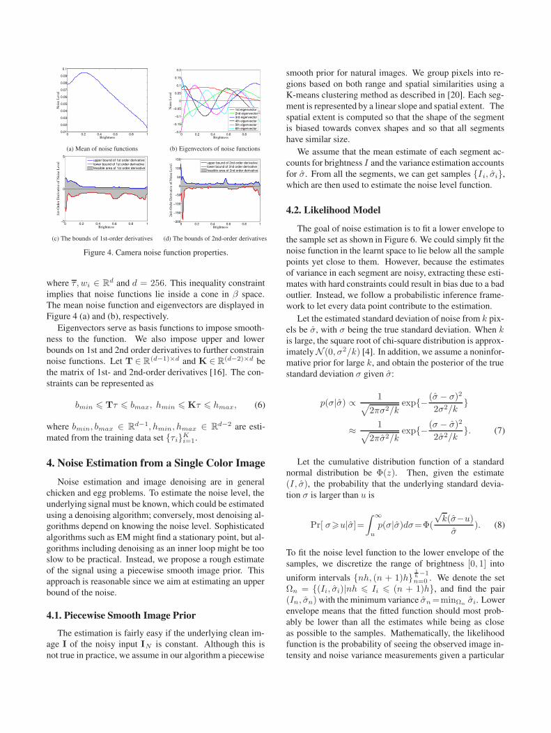
Figure 6. Synthesized noisy images and their corresponding noise
level functions (noise standard deviation as a function of image
brightness). The red, green and blue curves are estimated using the
proposed algorithm, whereas the gray curves are the true values for
the synthetically generated noise.
In the above formula, the matrix E=[w1 · · · wm] ∈ Rd×m
contains the principal components, en is the nth row of E,
and Λ = diag(v1, · · · , vm) is the diagonal eigenvalue ma-
trix. The last term in the objective function accounts for
the similarity of the NLF for RGB channels. Their similar-
ity is defined as a distance on 1st and 2nd order derivative.
Since the dimensionality of the optimization is low, we use
the MATLAB standard nonlinear constrained optimization
function fmincon for optimization. The function was able
to find an optimal solution for all the examples we tested.
5. Experimental Results
We have conducted experiments on both synthetic and
real noisy images to test the proposed algorithm. First, we
applied our CCD noise synthesis algorithm in Sect 3.3 to 17
randomly selected pictures from the Berkeley image seg-
mentation database [10] to generate synthetic test images.
To generate the synthetic CCD noise, we specify a CRF
and two parameters σs and σc. From this information, we
also produce the ground truth noise level function using the
training database in Sect 3.4. For this experiment, we se-
lected crf(60), σs = 0.10 and σc = 0.04. Then, we applied
our method to estimate the NLF from the synthesized noisy
images. Both L2 and L∞ norms are used to measure the
distance between the estimated NLF and the ground truth.
The error statistics under the two norms are listed in Table
1, where the mean and maximum value of the ground truth
are 0.0645 and 0.0932, respectively.
Some estimated NLFs are shown in Figure 6. In (a) we
observe many texture regions especially at high intensity
values, which implies high signal variance. The estimated
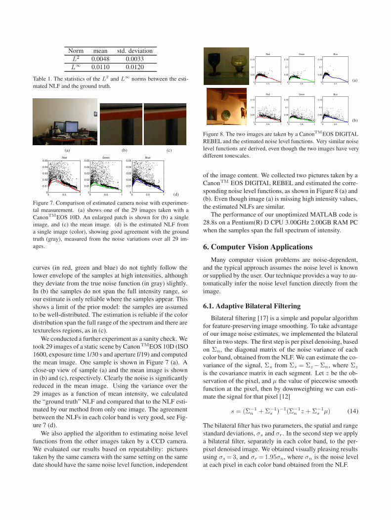
Norm mean std. deviation
L2 0.0048 0.0033
L∞ 0.0110 0.0120
Table 1. The statistics of the L2 and L∞ norms between the esti-
mated NLF and the ground truth.
(a) (b) (c)
0 0.5 10
0.01
0.02
0.03
0.04
0.05Red
0 0.5 10
0.01
0.02
0.03
0.04
0.05Green
0 0.5 10
0.01
0.02
0.03
0.04
0.05Blue
(d)
Figure 7. Comparison of estimated camera noise with experimen-
tal measurement. (a) shows one of the 29 images taken with a
CanonTMEOS 10D. An enlarged patch is shown for (b) a single
image, and (c) the mean image. (d) is the estimated NLF from
a single image (color), showing good agreement with the ground
truth (gray), measured from the noise variations over all 29 im-
ages.
curves (in red, green and blue) do not tightly follow the
lower envelope of the samples at high intensities, although
they deviate from the true noise function (in gray) slightly.
In (b) the samples do not span the full intensity range, so
our estimate is only reliable where the samples appear. This
shows a limit of the prior model: the samples are assumed
to be well-distributed. The estimation is reliable if the color
distribution span the full range of the spectrum and there are
textureless regions, as in (c).
We conducted a further experiment as a sanity check. We
took 29 images of a static scene by CanonTMEOS 10D (ISO
1600, exposure time 1/30 s and aperture f/19) and computed
the mean image. One sample is shown in Figure 7 (a). A
close-up view of sample (a) and the mean image is shown
in (b) and (c), respectively. Clearly the noise is significantly
reduced in the mean image. Using the variance over the
29 images as a function of mean intensity, we calculated
the “ground truth” NLF and compared that to the NLF esti-
mated by our method from only one image. The agreement
between the NLFs in each color band is very good, see Fig-
ure 7 (d).
We also applied the algorithm to estimating noise level
functions from the other images taken by a CCD camera.
We evaluated our results based on repeatability: pictures
taken by the same camera with the same setting on the same
date should have the same noise level function, independent
0 0.5 10
0.05
0.1
0.15
Red
0 0.5 10
0.05
0.1
0.15
Green
0 0.5 10
0.05
0.1
0.15
Blue
(a)
0 0.5 10
0.05
0.1
0.15
Red
0 0.5 10
0.05
0.1
0.15
Green
0 0.5 10
0.05
0.1
0.15
Blue
(b)
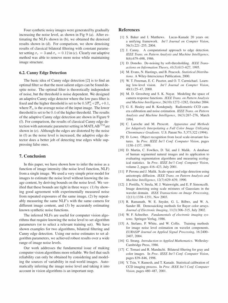
Figure 8. The two images are taken by a CanonTMEOS DIGITAL
REBEL and the estimated noise level functions. Very similar noise
level functions are derived, even though the two images have very
different tonescales.
of the image content. We collected two pictures taken by a
CanonTM EOS DIGITAL REBEL and estimated the corre-
sponding noise level functions, as shown in Figure 8 (a) and
(b). Even though image (a) is missing high intensity values,
the estimated NLFs are similar.
The performance of our unoptimized MATLAB code is
28.8s on a Pentium(R) D CPU 3.00GHz 2.00GB RAM PC
when the samples span the full spectrum of intensity.
6. Computer Vision Applications
Many computer vision problems are noise-dependent,
and the typical approach assumes the noise level is known
or supplied by the user. Our technique provides a way to au-
tomatically infer the noise level function directly from the
image.
6.1. Adaptive Bilateral Filtering
Bilateral filtering [17] is a simple and popular algorithm
for feature-preserving image smoothing. To take advantage
of our image noise estimates, we implemented the bilateral
filter in two steps. The first step is per pixel denoising, based
on Σn, the diagonal matrix of the noise variance of each
color band, obtained from the NLF. We can estimate the co-
variance of the signal, Σs from Σs = Σz −Σn, where Σz
is the covariance matrix in each segment. Let z be the ob-
servation of the pixel, and µ the value of piecewise smooth
function at the pixel, then by downweighting we can esti-
mate the signal for that pixel [12]
s = (Σ−1n + Σ−1
s )−1(Σ−1n z + Σ−1
s µ) (14)
The bilateral filter has two parameters, the spatial and range
standard deviations, σs and σr. In the second step we apply
a bilateral filter, separately in each color band, to the per-
pixel denoised image. We obtained visually pleasing results
using σs = 3, and σr = 1.95σn, where σn is the noise level
at each pixel in each color band obtained from the NLF.
Four synthetic noisy images were generated by gradually
increasing the noise level, as shown in Fig 9 (a). After es-
timating the NLFs shown in (b), we obtained the denoised
results shown in (d). For comparison, we show denoising
results of classical bilateral filtering with constant parame-
ter setting σr = 3 and σs = 0.12 in (c). Clearly our adaptive
method was able to remove more noise while maintaining
image structure.
6.2. Canny Edge Detection
The basic idea of Canny edge detection [2] is to find an
optimal filter so that the most salient edges can be found de-
spite noise. The optimal filter is theoretically independent
of noise, but the threshold is noise dependent. We designed
an adaptive Canny edge detector where the low pass filter is
fixed and the higher threshold is set to be 0.5σ2n+2σn+0.1,
where σn is the average noise of the input image. The lower
threshold is set to be 0.4 of the higher threshold. The results
of the adaptive Canny edge detection are shown in Figure 9
(f). For comparison, the results of classical Canny edge de-
tection with automatic parameter setting in MATLABTMare
shown in (e). Although the edges are distorted by the noise
in (f) as the noise level is increased, the adaptive edge de-
tector does a better job of detecting true edges while sup-
pressing false ones.
7. Conclusion
In this paper, we have shown how to infer the noise as a
function of image intensity (the noise level function, NLF)
from a single image. We used a very simple prior model for
images to estimate the noise level without knowing the im-
age content, by deriving bounds on the noise level. We ver-
ified that these bounds are tight in three ways: (1) by show-
ing good agreement with experimentally measured noise
from repeated exposures of the same image, (2) by repeat-
ably measuring the same NLF’s with the same camera for
different image content, and (3) by accurately estimating
known synthetic noise functions.
The inferred NLFs are useful for computer vision algo-
rithms that require knowing the noise level to set algorithm
parameters (or to select a relevant training set). We have
shown examples for two algorithms, bilateral filtering and
Canny edge detection. Using our noise estimates to set al-
gorithm parameters, we achieved robust results over a wide
range of image noise levels.
Our work addresses the fundamental issue of making
computer vision algorithms more reliable. We feel that such
reliability can only be obtained by considering and model-
ing the sources of variability in real-world images. Auto-
matically inferring the image noise level and taking it into
account in vision algorithms is an important step.
References
[1] S. Baker and I. Matthews. Lucas-Kanade 20 years on:
a unifying framework. Int’l Journal on Compter Vision,
56(3):221–255, 2004.
[2] J. Canny. A computational approach to edge detection.
IEEE Trans. on Pattern Analysis and Machine Intelligence,
8(6):679–698, 1986.
[3] D. Donoho. De-noising by soft-thresholding. IEEE Trans-
actions on Information Theory, 41(3):613–627, 1995.
[4] M. Evans, N. Hastings, and B. Peacock. Statistical Distribu-
tions. A Wiley-Interscience Publication, 2000.
[5] W. T. Freeman, E. C. Pasztor, and O. T. Carmichael. Learn-
ing low-level vision. Int’l Journal on Compter Vision,
40(1):25–47, 2000.
[6] M. D. Grossberg and S. K. Nayar. Modeling the space of
camera response functions. IEEE Trans. on Pattern Analysis
and Machine Intelligence, 26(10):1272–1282, October 2004.
[7] G. E. Healey and R. Kondepudy. Radiometric CCD cam-
era calibration and noise estimation. IEEE Trans. on Pattern
Analysis and Machine Intelligence, 16(3):267–276, March
1994.
[8] C. Laroche and M. Prescott. Apparatus and Methods
for Adaptively Interpolating a Full Color Image Utilizaing
Chrominance Gradients. U.S. Patent No. 5,373,322 (1994).
[9] D. Lowe. Object recognition from local scale-invariant fea-
tures. In Proc. IEEE Int’l Conf. Computer Vision, pages
1150–1157, 1999.
[10] D. Martin, C. Fowlkes, D. Tal, and J. Malik. A database
of human segmented natural images and its application to
evaluating segmentation algorithms and measuring ecolog-
ical statistics. In Proc. IEEE Int’l Conf. Computer Vision,
volume 2, pages 416–423, July 2001.
[11] P. Perona and J. Malik. Scale-space and edge detection using
anisotropic diffusion. IEEE Trans. on Pattern Analysis and
Machine Intelligence, 12(7):629–639, 1990.
[12] J. Portilla, V. Strela, M. J. Wainwright, and E. P. Simoncelli.
Image denoising using scale mixtures of Gaussians in the
wavelet domain. IEEE Transactions on Image Processing,
12(11):1338–1351, Nov 2003.
[13] R. Ramanath, W. E. Snyder, G. L. Bilbro, and W. A.
Sander III. Demosaicking methods for Bayer color arrays.
Journal of Electronic Imaging, 11(3):306–315, July 2002.
[14] W. F. Schreiber. Fundamentals of electronic imaging sys-
tems. Springer-Verlag, 1986.
[15] A. Stefano, P. White, and W. Collis. Training methods
for image noise level estimation on wavelet components.
EURASIP Journal on Applied Signal Processing, 16:2400–
2407, 2004.
[16] G. Strang. Introduction to Applied Mathematics. Wellesley-
Cambridge Press, 1986.
[17] C. Tomasi and R. Manduchi. Bilateral filtering for gray and
color images. In Proc. IEEE Int’l Conf. Computer Vision,
pages 839–846, 1998.
[18] Y. Tsin, V. Ramesh, and T. Kanade. Statistical calibration of
CCD imaging process. In Proc. IEEE Int’l Conf. Computer
Vision, pages 480–487, 2001.

(a)
0 0.5 10
0.05
0.1
0.15
Red
0 0.5 10
0.05
0.1
0.15
Green
0 0.5 10
0.05
0.1
0.15
Blue
0 0.5 10
0.05
0.1
0.15
0.2
Red
0 0.5 10
0.05
0.1
0.15
0.2
Green
0 0.5 10
0.05
0.1
0.15
0.2
Blue
0 0.5 10
0.05
0.1
0.15
0.2
Red
0 0.5 10
0.05
0.1
0.15
0.2
Green
0 0.5 10
0.05
0.1
0.15
0.2
Blue
0 0.5 10
0.05
0.1
0.15
0.2
Red
0 0.5 10
0.05
0.1
0.15
0.2
Green
0 0.5 10
0.05
0.1
0.15
0.2
Blue
(b)
(c)
(d)
(e)
(f)
(1) σs =0.030, σc =0.015 (2) σs =0.060, σc =0.030 (3) σs =0.090, σc =0.045 (4) σs =0.120, σc =0.060
Figure 9. Noise estimation can make computer vision algorithms more robust to noise. Four synthetic noise contaminated images (a) are
obtained by increasing σs and σc. Noise level functions as inferred by our algorithm from each image (b). (c) Classical bilateral filtering
with constant parameter setting. Note the sensitivity of the output to the input noise level. (d) Adaptive bilateral filtering exploiting inferred
noise levels, leading to robust performance independent of noise level. (e) Canny edge detection using the automatic parameter settings
supplied in MATLABTMprogram, which attempt to adapt to the input image. Despite adaptation, the algorithm does not adequately
compensate for the changes in image noise level. (f) Canny edge detection after adapting algorithm parameters using inferred noise level
functions. Algorithm performance is now substantially independent of the image noise levels.
[19] R. Zhang, P. Tsai, J. Cryer, and M. Shah. Shape from shad-
ing: A survey. IEEE Trans. on Pattern Analysis and Machine
Intelligence, 21(8):690–706, 1999.
[20] C. L. Zitnick, N. Jojic, and S. B. Kang. Consistent segmen-
tation for optical flow estimation. In Proc. IEEE Int’l Conf.
Computer Vision, pages 1308–1315, 2005.