PHASE NOISE ESTIMATION FOR WIRELESS COMMUNICATION SYSTEMS

BURC ARSLAN KALELI

Department of Electronics Engineering

APPROVED BY:

Prof. Dr. Erdal Panayırcı

Asst. Prof. Dr. Habib Senol

Asst. Prof. Dr. Hakan Dogan

APPROVAL DATE: 10/02/2011

PHASE NOISE ESTIMATION FOR WIRELESS COMMUNICATION SYSTEMS

by

BURC ARSLAN KALELI

THESIS

Presented to the Faculty of the Graduate School of

Kadir Has University

in Partial Fulfillment

of the Requirements

for the Degree of

MASTER OF SCIENCE

Department of Electronics Engineering

KADIR HAS UNIVERSITY

February 2011

PHASE NOISE ESTIMATION FOR WIRELESS

COMMUNICATION SYSTEMS

Abstract

In wireless communication systems information symbols are transmitted through a com-

munication channel which are affected many degradation factors. Besides fading and mul-

tipath effect of channel, transmitted symbols are significantly suffered from various noise

effects. Additive white Gaussian Noise (AWGN) is a well-known concept as noise which is

mentioned above and usually considered as only degradation while the signal is transmit-

ted. However, in certain circumstances, other degradation factors, for instance phase noise,

could be equally or more important. In this thesis, it is focused on phase noise problem

particularly.

Phase noise is rapidly time-varying and random disturbing effects on the phase of a

signal waveform. Presence of phase noise is increased symbol errors for overall system.

Therefore, this term must be eliminated in order to enhance the error performance. In

this thesis, it is considered the problem of joint detection of continuous-valued information

source output and estimation of a phase noise by using expectation maximization (EM)

algorithm. In order to estimate phase noise, initial phase noise values are determined by

cubic interpolation that utilizes pilot symbols.

In addition, computer simulations are performed for the proposed algorithm and the

average mean square error (MSE) - signal to noise ratio (SNR) performance of source de-

tector and phase noise estimator is presented for each iteration of the algorithm. Moreover,

average MSE - pilot spacing performance curves of phase noise estimator are given for

various SNR values.

iii

KABLOSUZ HABERLESME SISTEMLERI ICIN FAZ

GURULTUSU KESTIRIMI

Ozet

Kablosuz haberlesme sistemlerinde, bilgi sembolleri kanalda iletilirken cesitli bozucu etki-

lere maruz kalmaktadırlar. Kanalın sonumleme ve cok yollu iletim etkilerinin yanı sıra,

iletilen semboller cesitli gurultu etkileri tarafından onemli olcude bozunmaya ugramaktadır.

Bu bozucu gurultulerinden en cok bilineni toplamsal beyaz Gauss gurultusu olmakla be-

raber, sinyal iletimi sırasında genelde tek bozucu etki olarak degerlendirilmektedir. Fakat,

bazı durumlarda faz gurultusu gibi diger bozucu etkiler aynı olcude ya da daha onemli

olabilmektedir. Bu tezde, ozellikle faz gurultusu problemi uzerine calısılmıstır.

Faz gurultusu, bir dalga seklinin fazındaki ani, kısa sureli ve rastlantısal degisimini

niteleyen bozucu etkidir. Faz gurultusu etkisinin ortadan kaldırılması hata performansının

iyilisterilmesi adına oldukca onemlidir. Bu calısmada beklenti enbuyuklemesi (Expecta-

tion Maximization - EM) algoritması kullanılarak surekli-degerli bir enformasyon kaynagı

cıkısının sezimlenmesi ve cıkısı etkileyen bir faz gurultusunun kestirimi problemi uzerinde

durulmustur. Faz gurultusunun kestirimi icin gerekli baslangıc faz gurultusu degerleri pilot

simgelerden yararlanılarak kubik enterpolasyon yontemiyle olusturulmaktadır.

Ayrıca, onerilen algoritma icin bilgisayar benzetimleri yapılarak kaynak sezimleyicisi ve

faz gurultusu kestirimcisi icin ortalama karesel hata (Mean Square Error - MSE) - sinyal

gurultu oranı (Signal to Noise Ratio - SNR) basarımları algoritmanın her bir yineleme

adımı icin sunulmustur. Ayrıca, faz gurultusu kestirimcisinin ortalama karesel hata - pilot

aralıgı basarım egrileri cesitli sinyal gurultu oranları icin verilmistir.

iv

Acknowledgements

I would like to express my deep-felt gratitude to my advisor, Prof. Dr. Erdal Panayırcı,

the head of Electronics Engineering Department at Kadir Has University, for his constant

motivation, support, expert guidance, constant supervision and constructive suggestion for

the submission of my thesis work. He was never ceasing in his belief in me, always provid-

ing clear explanations when I was lost, and always giving me his time. I wish all students

would have an opportunity to experience his ability.

I also wish to thank Dr. Habib Senol of the Computer Engineering Department at

Kadir Has University. His suggestions and comments were invaluable to the completion

of this work. He was extremely helpful in providing the additional guidance and expertise

I needed, especially with regard to the chapter on phase noise estimation and simulation

results.

This thesis would have been impossible if not for the perpetual moral support from my

family and my friends. I would like to thank them all.

v

Table of Contents

Page

Abstract . . . . . . . . . . . . . . . . . . . . . . . . . . . . . . . . . . . . . . . . . . iii

Ozet . . . . . . . . . . . . . . . . . . . . . . . . . . . . . . . . . . . . . . . . . . . . iv

Acknowledgements . . . . . . . . . . . . . . . . . . . . . . . . . . . . . . . . . . . . v

Table of Contents . . . . . . . . . . . . . . . . . . . . . . . . . . . . . . . . . . . . . vi

List of Figures . . . . . . . . . . . . . . . . . . . . . . . . . . . . . . . . . . . . . . viii

Abbreviations . . . . . . . . . . . . . . . . . . . . . . . . . . . . . . . . . . . . . . . ix

Chapter

1 Introduction . . . . . . . . . . . . . . . . . . . . . . . . . . . . . . . . . . . . . . 1

1.1 A Brief History of Mobile Wireless networks . . . . . . . . . . . . . . . . . 2

1.2 Evolution of Wireless Local Area Networks to

Metropolitan Area Networks . . . . . . . . . . . . . . . . . . . . . . . . . . 3

1.3 The Challenges of Wireless Channels . . . . . . . . . . . . . . . . . . . . . 4

1.4 Phase Noise . . . . . . . . . . . . . . . . . . . . . . . . . . . . . . . . . . . 8

1.5 Objectives and Outline of Thesis . . . . . . . . . . . . . . . . . . . . . . . 10

2 Phase Noise . . . . . . . . . . . . . . . . . . . . . . . . . . . . . . . . . . . . . . 11

2.1 Introduction . . . . . . . . . . . . . . . . . . . . . . . . . . . . . . . . . . . 11

2.2 Mathematical Model of Phase Noise . . . . . . . . . . . . . . . . . . . . . . 12

2.3 Power Spectral Density of Phase Noise . . . . . . . . . . . . . . . . . . . . 13

3 Phase Noise Estimation . . . . . . . . . . . . . . . . . . . . . . . . . . . . . . . 15

3.1 Overview of Estimation Problem . . . . . . . . . . . . . . . . . . . . . . . 15

3.2 System Model . . . . . . . . . . . . . . . . . . . . . . . . . . . . . . . . . . 17

3.3 EM Based Phase Noise Estimation Algorithm . . . . . . . . . . . . . . . . 19

3.3.1 Expectation-Step (E-Step) . . . . . . . . . . . . . . . . . . . . . . . 19

3.3.2 Maximization-Step(M-Step) . . . . . . . . . . . . . . . . . . . . . . 21

vi

3.3.3 Initialization . . . . . . . . . . . . . . . . . . . . . . . . . . . . . . 23

4 Simulation Results . . . . . . . . . . . . . . . . . . . . . . . . . . . . . . . . . . 24

4.1 Phase Noise Estimator Performance . . . . . . . . . . . . . . . . . . . . . . 25

4.2 Source Detector Performance . . . . . . . . . . . . . . . . . . . . . . . . . 26

4.3 Optimum Pilot Interval . . . . . . . . . . . . . . . . . . . . . . . . . . . . . 27

5 Conclusion and Future Work . . . . . . . . . . . . . . . . . . . . . . . . . . . . . 28

5.1 Conclusion . . . . . . . . . . . . . . . . . . . . . . . . . . . . . . . . . . . . 28

5.2 Future Works . . . . . . . . . . . . . . . . . . . . . . . . . . . . . . . . . . 29

References . . . . . . . . . . . . . . . . . . . . . . . . . . . . . . . . . . . . . . . . . 30

Curriculum Vitae . . . . . . . . . . . . . . . . . . . . . . . . . . . . . . . . . . . . . 34

vii

List of Figures

1.1 Wireless Technologies . . . . . . . . . . . . . . . . . . . . . . . . . . . . . . 5

1.2 Digital Wireless Communication System . . . . . . . . . . . . . . . . . . . 6

1.3 Multipath Effect of Wireless Channel . . . . . . . . . . . . . . . . . . . . . 7

2.1 Lorentzian Power Spectral Density. . . . . . . . . . . . . . . . . . . . . . . 14

4.1 MSE Performance of Phase Noise Estimator. . . . . . . . . . . . . . . . . . 25

4.2 MSE Performance of Source Detector. . . . . . . . . . . . . . . . . . . . . . 26

4.3 MSE Performance of Phase Noise Estimator vs Pilot Interval. . . . . . . . 27

viii

Abbreviations

1G : First Generation

2G : Second Generation

3G : Third Generation

4G : Forth Generation

ADC : Analog to Digital Converter

AMPS : Advanced Mobile phone Service

AWGN : Additive White Gaussian Noise

CDMA : Code Division Multiple Access

DAC : Digital-to-Analog Converter

DCT : Discrete Cosine Transform

EDGE : Enhanced Data Rate for GSM Evolution

EM : Expectation Maximization

EVDO : Evolution Data Optimized

FDMA : Frequency Division Multiple Access

GMSK : Gaussian Minimum Shifting Key

GPRS : General Packet Radio Service

GSM : Global System for Mobile

HSDPA : High Speed Downlink Packet Access

ICI : Inter-carrier Interference

IEEE : The Institute of Electrical and Electronics Engineers

IP : Internet Protocol

ix

ISI : Inter-symbol Interference

LMMSE : Linear Minimum Mean Square Error

LTE : Long Term Evolution

MAN : Metropolitan Area Network

ML : Maximum Likelihood

MSE : Mean Square Error

NTT : Nippon Telephone and Telegraph

NMT : Nordic Mobile Telephone

OFDM : Orthogonal Frequency Division Multiplexing

PLL : Phase Locked Loop

QoS : Quality of Service

RF : Radio Frequency

SNR : Signal to Noise Ratio

TDMA : Time Division Multiple Access

UMTS : Universal Mobile Telecommunication System

WiMAX : Worldwide Interoperability for Microwave Access

WLAN : Wireless Local Area Network

x

Chapter 1

Introduction

At the beginning of 90’s, digital communication experienced a fast growth with the im-

pact of the internet. From 1990 to 2009 the Internet grew from zero to two billion users

and wireless mobile services grew from 10 million to 4.5 billion subscribers in 2009 around

worldwide [1]. This rapid growth of the Internet is initiating the demand for higher speed

Internet based services which is leading to growth of broadband wireless systems. In a short

time, worldwide subscription for broadband wireless services reached over 480 million [1].

It’s inevitable that these technologies, which were considered as luxury in previous years,

are now essential and necessary. In other words, within the last two decades, communica-

tion advances have changed our life.

Our lives are still changing according to the developments and becoming increasingly

dependent on mobile communication. Besides, user demands go beyond to simple speech

transmission to ”reach and share information everywhere and every time”. This demand

has directed the future of mobile and wireless communications towards to provide services

without regard to location with high data rates. To achieve this goal, communication net-

works need to be support wide range of services which includes high quality voice, still

images, streaming videos and high data rate applications. Therefore, this is obvious that,

next generation communication systems will be defined as a combination of Internet and

Multimedia communications and wireless mobile communications to achieve high data rates

and high coverage concurrently.

However, this is a quite difficult problem. Local area networks supports high data rates

1

for limited coverage. On the other hand, wireless mobile communication networks, namely

cellular systems, supports low data rate services for high coverage area. The main problem

is to design a system that services many users at high data rates with conceivable band-

width and acceptable power consumption which also enables high coverage and quality of

service (QoS).

To cope with this problem, many different transmission techniques are proposed over

time. Currently, some of these techniques are actively under development. In this thesis,

phase noise estimation problem is considered, particularly, for basic single carrier transmis-

sion systems.

1.1 A Brief History of Mobile Wireless networks

The first commercial mobile communication systems, which are based on analog cellular

technology, were developed in the 80’s, such as advanced mobile phone service (AMPS) in

the USA, Nippon Telephone and Telegraph (NTT) in Japan and Nordic Mobile Telephone

(NMT) in Norway etc. These systems ensured only speech transmission and almost each

country offered its own system, naturally there were an incompatibility between them. Be-

sides, call capacity of these analog systems were limited and quality of speech were not

good enough. These systems were the first steps of mobile communication and called first

generation (1G) communication systems.

The second generation (2G) technology is based on digital cellular technology. The

most well-known 2G service is Global System for Mobile (GSM) which is started its opera-

tions in Finland in 1992. Unlike 1G, 2G systems commonly used more efficient modulation

techniques to provide better quality of speech. For instance, GSM used 2-Level Gaussian

Minimum Shifting Key (GMSK). 2G also used multiplexing technologies such as, time

division multiple access (TDMA), frequency division multiple access (FDMA) and code

2

division multiple access (CDMA) to ensure the coordinated access between multiple users.

Thus, the call capacity of the system is increased. At last stages, two services which are

general packet radio service (GPRS) and enhanced data rate for GSM evolution (EDGE)

are developed in order to provide more data rates. These technologies are overlaid on cur-

rent 2G technologies and called 2.5G. [2]

Appearance of higher demand for data services are initialized the development of third

generation (3G) networks, namely multimedia support. Two main technologies are devel-

oped within 3G concept which are Universal mobile telecommunication system (UMTS)

and CDMA2000. Though some enhancements such as evolution data optimized (1xEVDO)

for CDMA2000 and high speed downlink packet access (HSDPA) for UMTS high data rates

are provided for users.

Currently, fourth generation (4G) wireless networks are under development. 4G is

defined as internet protocol (IP) Packet switching network which provides higher data

rates and higher capacity. Main goal of 4G is to replace the current cellular networks with

a single worldwide cellular core network standard based on IP for voice, video and data

services [3]. Some services such as mobile Worldwide Interoperability for Microwave Access

(WiMAX) and first release long term evolution (LTE)

1.2 Evolution of Wireless Local Area Networks to

Metropolitan Area Networks

As it is seen from previous section, the first mobile wireless systems aren’t designed for data

services because internet concept was still immature. The design objectives of wireless lo-

cal area networks (WLAN) are completely different than mobile wireless networks, namely

high data throughput is more important than mobility. The IEEE 802.11 is standardized

3

in 1997 and provided users 2 Mbps data rate [2]. After that, several amendments are made

this standard and capabilities are increased.

However, despite high data rates, coverage was an important drawback for WLAN’s

because these systems are designed for connectivity in office or home environments. A new

technology is clearly needed to provide high throughput broadband connection over large

areas for fixed or mobile users. For this reason WiMAX standard is developed by IEEE

802.16 metropolitan area network (MAN) research group.

When evolution of mobile wireless networks and wireless local area networks is consid-

ered, there still exists a big gap between the mobility offered by mobile wireless networks

and high data rates offered by WLAN technology. As mentioned in previous section, this

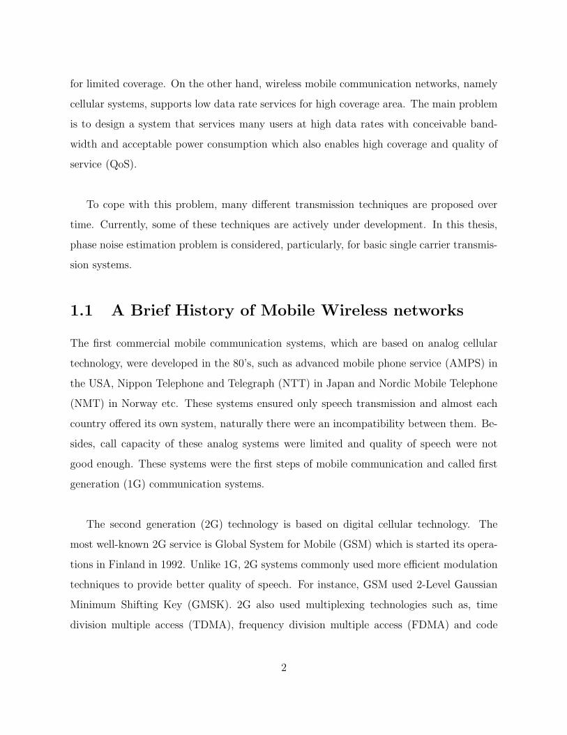
intersection point is directed to 4G researches as shown in figure 1.1.

1.3 The Challenges of Wireless Channels

All wireless digital communication systems possess several functional blocks similar to dig-

ital communication systems as shown in the figure 1.2. Even if a wireless network is

complicated, the entire system can be expressed as a collection of links which are transmit-

ter, channel and receiver.

The main function of the transmitter is, to receive data from higher protocol layer and

send them to receiver as electromagnetic waves. The important parts of the digital domain

are encoding (source and channel respectively) and modulation. The function of the source

encoder is to represent the data by bits in efficient way. On the other hand, channel encoder

adds redundant bits to data which enable detection and correction of transmission errors

in the receiver. The modulator prepares the data for wireless channel by grouping and

transforming to certain symbols or waveforms. The modulated signal is converted into a

4

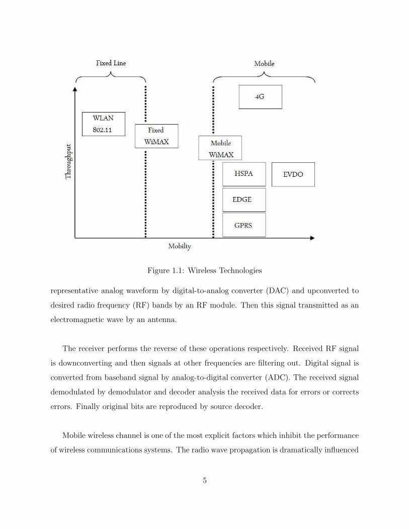
Figure 1.1: Wireless Technologies

representative analog waveform by digital-to-analog converter (DAC) and upconverted to

desired radio frequency (RF) bands by an RF module. Then this signal transmitted as an

electromagnetic wave by an antenna.

The receiver performs the reverse of these operations respectively. Received RF signal

is downconverting and then signals at other frequencies are filtering out. Digital signal is

converted from baseband signal by analog-to-digital converter (ADC). The received signal

demodulated by demodulator and decoder analysis the received data for errors or corrects

errors. Finally original bits are reproduced by source decoder.

Mobile wireless channel is one of the most explicit factors which inhibit the performance

of wireless communications systems. The radio wave propagation is dramatically influenced

5

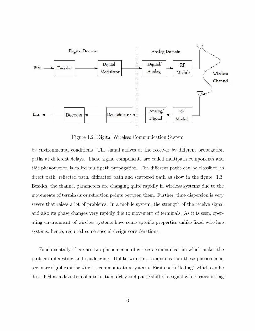
Figure 1.2: Digital Wireless Communication System

by environmental conditions. The signal arrives at the receiver by different propagation

paths at different delays. These signal components are called multipath components and

this phenomenon is called multipath propagation. The different paths can be classified as

direct path, reflected path, diffracted path and scattered path as show in the figure 1.3.

Besides, the channel parameters are changing quite rapidly in wireless systems due to the

movements of terminals or reflection points between them. Further, time dispersion is very

severe that raises a lot of problems. In a mobile system, the strength of the receive signal

and also its phase changes very rapidly due to movement of terminals. As it is seen, oper-

ating environment of wireless systems have some specific properties unlike fixed wire-line

systems, hence, required some special design considerations.

Fundamentally, there are two phenomenon of wireless communication which makes the

problem interesting and challenging. Unlike wire-line communication these phenomenon

are more significant for wireless communication systems. First one is ”fading” which can be

described as a deviation of attenuation, delay and phase shift of a signal while transmitting

6

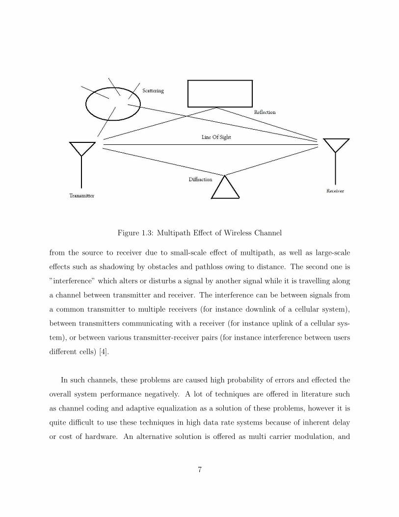
Figure 1.3: Multipath Effect of Wireless Channel

from the source to receiver due to small-scale effect of multipath, as well as large-scale

effects such as shadowing by obstacles and pathloss owing to distance. The second one is

”interference” which alters or disturbs a signal by another signal while it is travelling along

a channel between transmitter and receiver. The interference can be between signals from

a common transmitter to multiple receivers (for instance downlink of a cellular system),

between transmitters communicating with a receiver (for instance uplink of a cellular sys-

tem), or between various transmitter-receiver pairs (for instance interference between users

different cells) [4].

In such channels, these problems are caused high probability of errors and effected the

overall system performance negatively. A lot of techniques are offered in literature such

as channel coding and adaptive equalization as a solution of these problems, however it is

quite difficult to use these techniques in high data rate systems because of inherent delay

or cost of hardware. An alternative solution is offered as multi carrier modulation, and

7

orthogonal frequency division multiplexing (OFDM) is appeared one of the appropriate

technique which is proposed in 1966 [5].

However, one of the biggest problem is phase noise sensitivity for all proposed techniques

either single carrier and multi carrier systems. Therefore, phase noise estimation problem

is considered in this thesis.

1.4 Phase Noise

Rapidly time-varying and random disturbing effects on the phase of a signal waveform are

known as phase noise [6]. This problem occurs in early stages of receiver part, especially

in demodulation stage. The time-varying multiplicative effects such as, Doppler Shifts and

oscillator jitter, and synchronization problems between the transmitter and receiver, can

be considered as basic reasons of phase noise. These disturbances can effects the overall

performance of the communication system by degrading the error performance, therefore

phase noise estimation has critical importance.

In literature, there are several methods exist for phase noise estimation. This problem

was solved by a feedback algorithm that operated according to Phase Locked Loop (PLL)

mechanism a long time ago [7], [8]. However, these algorithms are not appropriate for burst

transmission in order to needed long acquisition periods. In addition, most of such PLL’s

are designed in analog form and would be needed may operations for digital conversation.

In the other approach, phase noise is approximated as piecewise constant over an ob-

servation interval. Therefore, a feedforward algorithm can be used to estimate the local

time average of phase in order to assumed constant in each subintervals [8], [9]. However,

subintervals have to be small for strong phase noise in which case the phase noise estimate

is sensitive to the channel noise.

8

Other significant results are obtained by a linear minimum mean square error (LMMSE)

estimation algorithm for a single carrier broadband system which is using Wiener filters

proposed in [10] for stationary model of phase noise. This is one of the easiest but subop-

timum solution because neglects all spatial correlations for each noise process. In addition,

for the estimation of a temporally non-stationary random phase noise sequences which

have a low magnitude with compared to symbol rate, such as Wiener phase noise, various

approaches can be found in literature [11, 17].

Recently, one of the popular method which is used for the iterative estimation of Markov-

type phase noise is a sum product algorithm and factor graph framework proposed in [18].

However, in this research it is assumed that receiver has detailed knowledge about phase

noise statistics. Therefore, this algorithm seems quite inadequate for real applications.

In [19], [20], discrete cosine transform (DCT) based basis expansion model is applied for

phase noise estimation from pilot symbols. Additionally, in [21] same pilot base algorithm

is used for initial estimation of phase noise, and then an iterative algorithm is used by mak-

ing of soft decisions of the unknown data symbols to improve this estimation. Maximum

likelihood (ML) algorithm is also used in [22] for the estimation of the average of the phase

noise over a block of data. However, random variations of the phase are neglected in the

algorithm.

It is mentioned in section 1.3 that OFDM is chosen as basis technique for next genera-

tion wireless systems, because of high spectral efficiency and ability to divide a dispersive

multipath channel into parallel frequency flat subchannels. Moreover, by applying a cyclic

prefix is also protected the OFDM symbol from delayed version of previous symbol and

cancelled inter-symbol interference (ISI). However, the performance of an OFDM system

can also be significantly degraded by the presence of random phase noise because it effects

9

the orthogonality between subcarriers and occured inter-carrier interference (ICI). This

sensitivity is one of the major drawbacks of OFDM. The effect of phase noise on the per-

formance of an OFDM system is also strongly concerned in the literature [23, 27].

1.5 Objectives and Outline of Thesis

In this thesis, phase noise estimation problem for wireless communication systems is deeply

investigated. The main objective of this research is to construct an effective and low com-

plexity phase noise estimation algorithm unlike proposed in literature for a wireless commu-

nication system which is affected by a strong phase noise. In addition, suggested algorithm

and the existing algorithms are compared with respect to computational complexity, and

the usefulness of proposed scheme is discussed.

The algorithm, mentioned above, is performed by MATLAB simulations and MSE vs

SNR performance is obtained. Besides these, detection of information source output has

an importance in algorithm. In the context of this research, a detector is designed and

performed by MATLAB simulations. At last, average MSE - pilot spacing performance

curves of phase noise estimator are studied for various SNR values.

The thesis organized as follows: in Chapter 2, the basics of phase noise are presented. It

is explained that reasons and characteristics of phase noise, and its mathematical model. In

chapter 3, system model and proposed algorithm is presented. Chapter 4 demonstrates the

simulation results of proposed algorithm and chapter 5 concludes the thesis and summarizes

the results of the work. Future works are also suggested.

10

Chapter 2

Phase Noise

2.1 Introduction

AWGN channel is a well-known concept for everyone who has taken digital communication

courses. Conventionally, this is usually considered as only degradation while the signal is

transmitted. In general, white Gaussian noise comes from many natural sources such as

thermal noise which is vibrations of atoms or black body radiation from the earth and other

warm objects. Human made noises are also considered as white noise. White means that

frequency spectrum is continuous and uniform for all frequency bands. In addition, it is

additive because signal is statistically independent from noise, and obviously noise samples

have Gaussian distribution. In the time domain Additive White Gaussian noise, which is

denoted n(t) ,can be shown as,

r(t) = Asin(2πfc + φ) + n(t), (2.1)

where A is the amplitude and φ is a constant that represents arbitrary phase offset. fc is

center frequency of the oscillator.

The AWGN channel is a good and sufficient model for many conditions however, in

certain circumstances, other degradation factors could be equally or more important. For

instance, fading, co-channel interference, antenna efficiency and phase noise. Particularly,

a communication systems which is effected by a phase noise (θ) is considered therefore, in

general, the output of oscillator with phase noise is can be written as,

11

r(t) = Asin(2πfc + θ(t) + φ) + n(t). (2.2)

Phase noise is one of the biggest difficulties in communication systems and phase noise

estimation problem has a great importance. The carrier phase must be known at the

receiver stage for the recovery of transmitted symbols. Therefore, the phase term which is

disturbed due to the synchronization problem between the transmitter and receiver, and

Doppler shifts problems, must be eliminated. Unlike white Gaussian noise, phase noise is

residual and time varying.

2.2 Mathematical Model of Phase Noise

In the literature, early studies on phase noise are focused on fiber optical communication

and later on radio oscillators. Since these early studies, the most accepted model for phase

noise θ(t) is a Wiener process. This model initially derived empirically and then analyti-

cally showed that it is accurate. For more information about phase noise modeling process

referred to [28] and [29]. In addition to Wiener process model, there are a lot of complex

models are proposed in literature to describe the phase noise process both in fiber and radio

communications [30]. However, because of the simplicity of Wiener Process and sufficiency

of describing phase noise process, this model is used in literature.

The phase noise θ(t) is modeled as wiener process,

θ(t) = 2π

∫ t

0

u(t)dt for (t > 0), (2.3)

where u(t) is a zero mean white Gaussian noise process. In case of N0 is defined as double

sided power spectral density of u(t), the variance of θ(n) which is zero-mean Gaussian

process,

var[θ(t)] = (2π)2N0t. (2.4)

12

As seen from (2.4), as t increases in time, the variance of θ(t) also increases concurrently.

Therefore, the phase of s(t) is clearly a random variable uniformly distributed over [0, 2π).

It is obvious that, estimation of these random variables are quite difficult. There already

exist a lot of estimation algorithms for this challenging problem and most of them achieve

a good performance under their design conditions. In next chapter, a novel approach for

this estimation problem is presented.

2.3 Power Spectral Density of Phase Noise

Power spectral density describes the distribution of power of a signal for each frequency

in spectrum. It is well-known that white noise has a flat power spectral density, namely,

contains equal power within a fixed bandwidth at any center frequency. However, this

situation is different for phase noise. The Fourier transform pair gives the spectrum of

pure cosine wave as,

cos(2πfot) ⇔1

2[δ(f − fo) + δ(f + fo)]. (2.5)

When (2.2) is checked, it is clearly seen that r(t) is a noise process itself because of

noise process θ(t) is added directly to this term. Therefore, the power spectrum can be

calculate as a Fourier transform of the autocorrelation function,

Rss(t, t+ τ) = E[y(t)y(t+ τ)]. (2.6)

Here, r(t) is nonstationary if φ has fixed value which is a known constant. However, in

real systems φ is totally random therefore, during mathematical modeling φ is assumed as

a random variable. If φ is chosen as uniformly distributed over [0, 2π), then autocorrelation

function can be calculated since r(t) is stationary. We find that Rss(t, t+ τ) = Rss(τ),

Rss(τ) =A2

2cos(2πfoτ)e

−2π2N0|τ |. (2.7)

13

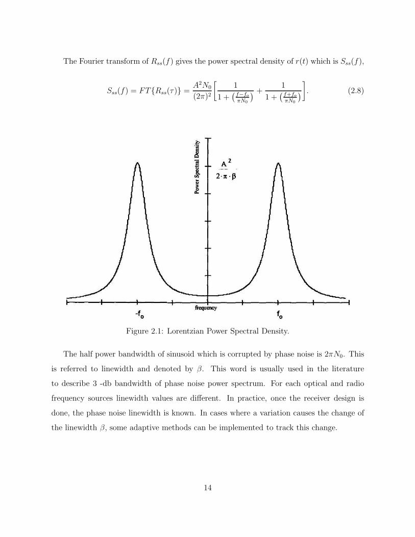
The Fourier transform of Rss(f) gives the power spectral density of r(t) which is Sss(f),

Sss(f) = FT{Rss(τ)} =A2N0

(2π)2

[1

1 +(f−foπN0

) +1

1 +(f+foπN0

)]. (2.8)

Figure 2.1: Lorentzian Power Spectral Density.

The half power bandwidth of sinusoid which is corrupted by phase noise is 2πN0. This

is referred to linewidth and denoted by β. This word is usually used in the literature

to describe 3 -db bandwidth of phase noise power spectrum. For each optical and radio

frequency sources linewidth values are different. In practice, once the receiver design is

done, the phase noise linewidth is known. In cases where a variation causes the change of

the linewidth β, some adaptive methods can be implemented to track this change.

14

Chapter 3

Phase Noise Estimation

As indicated previous chapters, wireless communication systems need an accurate time

reference because of their structure. Various users share same channel, necessitating mod-

ulation and demodulation of the messages in these systems. In addition, reliable modulation

and demodulation is highly dependent on accuracy of oscillators. Furthermore, in order to

reach desired high data rates in next generation high speed communication systems, this

accuracy has an important role because the frequency instabilities of the carrier degrades

the overall performance of the system. Therefore, an effective phase noise estimation is con-

siderably important to cope with this problem and enhance the performance of systems. In

this thesis, an optimal phase noise estimation algorithm is generated for continuous-valued

data transmission which is affected by a phase noise.

In this chapter, after the estimation problem is briefly examined ,the system model and

also system parameters are given which are used in the model are presented. In addition,

developed phase noise estimation algorithm is introduced step by step and details about

EM based estimation is given in the rest of the chapter.

3.1 Overview of Estimation Problem

As it is known that estimation is a large concept which is at the heart of many signal

processing systems such as, communications, biomedicine and seismology etc. Carrier

frequency estimation or phase noise estimation in communication; estimation of the heart

rate of a fetus in biomedicine; or estimation of the underground distance of an oil can

15

be good example. Obviously seen that the common problem here is needing to estimate

the values of a group of parameters. In the simplest form, we have the N point data set

{x[0], x[1], x[2], ..., x[N − 1]} which depends on an unknown parameter θ. Therefore, we

would like to determine θ based on the data or to define an estimator[31],

θ = g(x[0], x[1], x[2], ..., x[N − 1])

where, g is some function. This is the basic mathematical model of parameter estima-

tion problem. For this problem, let’s consider the receiver side observation relation of a

communication system in order to estimate unknown θ parameter vector as follows:

y = F(s, θ) +w

where, y is observation vector, s is nuisance parameter vector and w is additive Gaussian

noise vector in that model. A maximum-likelihood estimation of θ vector is based on

maximization of θ according to p(y|θ) = Es[p(y|s, θ)] probability function and can be

defined mathematically as follows,

θML = argmaxθ

p(y|θ) = argmaxθ

Esp(y|θ, s). (3.1)

Here, Es{.} denotes the expected value with respect to s. As seen from (3.1) equation,

maximum likelihood estimation can be performed after the following two basic steps,

1) Calculating the statistical average over s nuisance parameter vector, in or-

der to compute the likelihood function. However, this may be analytically

intractable

2) Maximization of likelihood function over unknown θ vector.Even if the likeli-

hood can be obtained analytically, however, it is invariably a nonlinear function

of s. Therefore, maximization step is computationally infeasible because it must

be performed in real time.

16

In such cases and under some conditions, the EM algorithm based phase noise estima-

tion may provide an implementable solution. There are many different problems are solved

by the use of EM algorithm in the literature [32, 33, 34, 35].

3.2 System Model

In this thesis, the transmission of a data block which contains N symbols is considered over

an AWGN channel which is affected by a phase noise. The phase noise is modeled as a

discrete - time Wiener process which is given by,

θ(n) = θ(n− 1) + u(n), n = 0, 1, · · · , N−1 ,

θ(−1) = 0, (3.2)

Here, u(n) represents a sequence of independent and identically distributed (i.i.d) zero-

mean Gaussian random variables with variance σ2u. The resulting received signal model can

be defined as,

y(n) = ejθ(n)s(n) + w(n) , n = 0, 1, · · · , N−1 , (3.3)

Vectorial definition of this expression can be more easy and more useful in future cal-

culations. Therefore, (3.2) and (3.3) can be defined in vectorial form as,

θ = Gu

y = Ψs+w . (3.4)

Where,

17

y = [y(0), y(1), · · · , y(N − 1)]T ,

s = [s(0), s(1), · · · , s(N − 1)]T ∼ CN (sP ,Σ(0)s ),

θ = [θ(0), θ(1), · · · , θ(N − 1)]T ∼ N (0,Σθ),

u = [u(0), u(1), · · · , u(N − 1)]T ∼ CN (0, σ2uIN),

w = [w(0), w(1), · · · , w(N − 1)]T ∼ CN (0, N0IN),

describes received signal vector, source signal vector, phase noise vector, Wiener phase pro-

cess noise vector and additive white noise vector of channel respectively. Here, IN denotes

N × N identity matrix. In addition, it is defined as η = [ejθ(0), ejθ(1), · · · , ejθ(N−1)]T and

diag(·) operator shows obtaining a diagonal matrix from a given vector. In this case, it is

obtained as Ψ = diag(η). G matrix, which is in (3.4) model, is expressed as,

G =

1 0 · · · 01. . .

. . ....

.... . .

. . . 0

1· · · 1 1

(3.5)

and, correspondingly covariance matrix of phase noise vector is calculated as follows,

Σθ = σ2uGGT = σ2

u

1 1 1 · · · 1

1 2 2 · · · 2

1 2 3 · · · 3...

......

. . ....

1 2 3 · · · N

(3.6)

Besides, source signal vector s,

18

s(n) =

sp(n) , n ∈ {0,∆, 2∆, · · · , (P − 1)∆}

sd(n) , otherwise

n = 0, 1, · · · , N − 1 (3.7)

is obtained by addition of pilot and data vectors, in other words s = sp + sd. Here, ∆

denotes pilot interval and P indicates pilot number in s vector.

3.3 EM Based Phase Noise Estimation Algorithm

The EM algorithm is an iterative method which enables approximating the ML estimation

when the direct computation is computationally prohibitive because of missing or hidden

data. In other words, EM algorithm is a generalization of ML estimation to the incom-

plete data case. Each iteration of the algorithm consists of two processes respectively: The

expectation step (E-Step) and maximization step (M-step). In the E-step expectation of

log-likelihood function is calculated according to distribution of missing or hidden data in

the model. Afterwards, in the M-step, the iteration based update rule is obtained which

maximizes the parameter of the expectation of log-likelihood function. These steps can

detailed as follows,

3.3.1 Expectation-Step (E-Step)

First step of EM algorithm is guessing a probability distribution over completions of miss-

ing data given the current model. Therefore, E-step of the algorithm calculates the function

given below,

Q(θ|θ(i)) = Es{ln p(θ|y, s)|y, θ(i)}. (3.8)

19

Since maximization is performed with respect to θ in M-Step, unnecessary terms which

are not dependent on θ can easily removed and expressed as below,

ln p(θ|y, s) ∼ ln p(y|θ, s) + ln p(θ), (3.9)

After substituting (3.9) into (3.8), the following expression of Q(θ|θ(i)) is easily ob-

tained,

Q(θ|θ(i)) ∼ Es{ln p(y|θ, s)|y, θ(i)}+ ln p(θ) (3.10)

Expected value of given (3.10) expression’s right hand side can be obtained by using

the receive signal model in (3.4)and after unnecessary terms which are not dependent on

θ are removed as shown below,

Es{ln p(y|θ, s)|y, θ(i)} ∼

1

N0

[y†Ψµ

(i)s + µ

(i)†

s Ψ†y]

(3.11)

Here, µ(i)s indicates a posteriori expected value of s vector for given θ(i) and expressed

as following,

µ(i)s = E{s|y, θ(i)}

= sp +1

N0Σ

(i)s Ψ(i)†

(y −Ψ(i)sp

)(3.12)

In this expression, Σ(i)s indicates a posteriori covariance matrix of s for given θ(i) and

expressed as shown below,

20

Σ(i)s = E{ss†|y, θ(i)}

= Σ(0)s

(IN +

1

N0

Σ(0)s

)−1

(3.13)

In addition, Σ(0)s indicates a priori covariance matrix of s vector. It is also known that

θ ∼ N(0,Σθ) from (3.4) and Σθ matrix is also given in (3.6) expression. Therefore, log-

likelihood function θ can be expressed as,

ln p(θ) ∼ −θTΣ−1

θθ (3.14)

Finally, Q(θ|θ(i)) function can be obtained by substituting (3.11) and (3.14) expressions

into (3.10),

Q(θ|θ(i)) ∼1

N0[y†Ψµ

(i)s + µ

(i)†

s Ψ†y]− θTΣ−1

θθ (3.15)

3.3.2 Maximization-Step(M-Step)

In the M-step of the algorithm the log-likelihood function is maximized under the assump-

tion that the missing data are known. The estimate of the missing data from the E-step

are used instead of the actual missing data. Therefore, in this step, expected value of log-

likelihood function in (3.8) is maximized with respect to θ and updating rule is presented

for phase noise estimation.

θ(i+1) = argmaxθ

Q(θ|θ(i)) (3.16)

Q(θ|θ(i)) function which is obtained in (3.15) is maximized with respect to θ as shown

below:

21

∂Q(θ|θ(i))

∂θ

∣∣∣θ=θ

(i+1) =−2

N0Im

[diag(y∗ ⊙ µ

(i)s )η(i+1)

]

−2Σ−1

θθ(i+1)

=0. (3.17)

Here, (·)∗ denotes complex conjugate operation and⊙ denotes element by element multi-

plication. In addition, it is defined as follows η(i+1) = [ejθ(i+1)(0), ejθ

(i+1)(1), · · · , ejθ(i+1)(N−1)]T .

In general, because of |θ(n)| ≪ 1, η(n) = ejθ(n) function can expand to taylor series over

θ(n) for θ(n). Therefore, it is obtained the linear approach of η(n) by taking the first two

term of expansion as shown below,

η(n) = ejθ(n) , n = 0, 1, · · · , N − 1

∼= ejθ(n) + j[θ(n)− θ(n)

]ejθ(n)

= [1− jθ(n)]ejθ(n) + jejθ(n) θ(n), (3.18)

(3.18) expression can be rearranged by taking θ(n) = θ(i+1)(n) and θ(n) = θ(i)(n) in

this approach with given definitions a(i)(n) = [1− jθ(i)(n)]ejθ(i)(n), b(i)(n) = jejθ

(i)(n) :

η(i+1)(n) ∼= a(i)(n) + b(i)(n) θ(i+1)(n). (3.19)

(3.19) expression can be obtained as a vector with the given definitions

a(i) = [a(i)(0), a(i)(1), · · · , a(i)(N−1)]T and b(i) = [b(i)(0), b(i)(1), · · · , b(i)(N−1)]T as follows:

η(i+1) ∼= a(i) + diag(b(i)) θ(i+1). (3.20)

22

Finally, updating rule for phase noise estimation is obtained by substituting (3.20) ex-

pression into (3.17) expression as shown below:

θ(i+1) = −T (i)−1v(i). (3.21)

Here, T (i) matrix and v(i) vector are defined as,

T (i) =(Im

[diag(y∗ ⊙ µ

(i)s ⊙ b(i))

]+N0Σ

−1

θ

)−1

,

v(i) = Im[diag(y∗ ⊙ µ

(i)s )a(i)

](3.22)

3.3.3 Initialization

At first step, the pilot symbols are employed as observations. To obtain an initial estimate,

phase noise values are calculated at receiver as shown below,

θ(0)(n) = arg( y(n)

sp(n)

), n ∈ {0,∆, 2∆, · · · , (P − 1)∆}. (3.23)

Therefore, initial phase noise values in data positions are determined by cubic interpo-

lation of initial pilot position values which are given in (3.23).

23

Chapter 4

Simulation Results

As mentioned in first chapter, there are various methods are proposed in literature for

phase noise estimation. However, researches on this problem still continue because ob-

tained results are not satisfactory. Therefore, after theoretical framework is provided for

suggested algorithm, performance of this algorithm is presented by computer simulations

in this chapter. In order to evaluate the performance of phase noise estimation and source

detection algorithms, MSE curves were used. For the simulations in this project, MATLAB

was employed with its Communications Toolbox for all data runs.

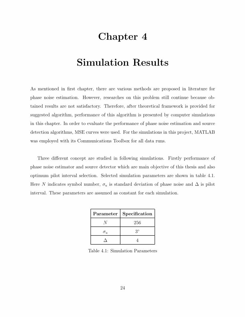
Three different concept are studied in following simulations. Firstly performance of

phase noise estimator and source detector which are main objective of this thesis and also

optimum pilot interval selection. Selected simulation parameters are shown in table 4.1.

Here N indicates symbol number, σu is standard deviation of phase noise and ∆ is pilot

interval. These parameters are assumed as constant for each simulation.

Parameter Specification

N 256

σu 3◦

∆ 4

Table 4.1: Simulation Parameters

24

4.1 Phase Noise Estimator Performance

In this section, the performance of the proposed algorithm in terms of the MSE of the phase

estimation is shown by computer simulations. It is assumed the transmission of a block

of N symbols over an AWGN channel in the presence of Wiener phase noise θ(n) which is

described in (3.2)

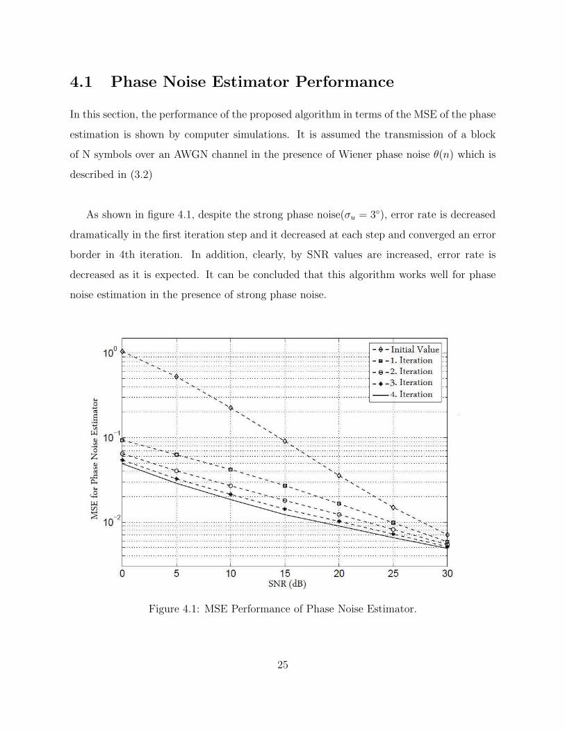
As shown in figure 4.1, despite the strong phase noise(σu = 3◦), error rate is decreased

dramatically in the first iteration step and it decreased at each step and converged an error

border in 4th iteration. In addition, clearly, by SNR values are increased, error rate is

decreased as it is expected. It can be concluded that this algorithm works well for phase

noise estimation in the presence of strong phase noise.

Figure 4.1: MSE Performance of Phase Noise Estimator.

25

4.2 Source Detector Performance

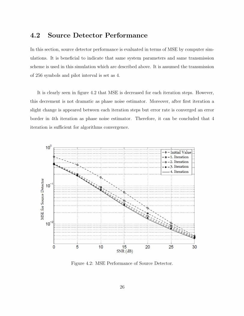
In this section, source detector performance is evaluated in terms of MSE by computer sim-

ulations. It is beneficial to indicate that same system parameters and same transmission

scheme is used in this simulation which are described above. It is assumed the transmission

of 256 symbols and pilot interval is set as 4.

It is clearly seen in figure 4.2 that MSE is decreased for each iteration steps. However,

this decrement is not dramatic as phase noise estimator. Moreover, after first iteration a

slight change is appeared between each iteration steps but error rate is converged an error

border in 4th iteration as phase noise estimator. Therefore, it can be concluded that 4

iteration is sufficient for algorithms convergence.

Figure 4.2: MSE Performance of Source Detector.

26

4.3 Optimum Pilot Interval

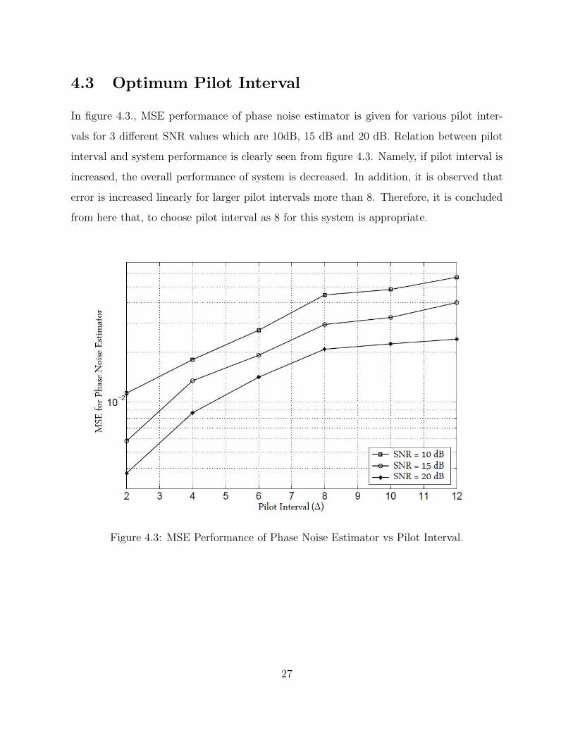
In figure 4.3., MSE performance of phase noise estimator is given for various pilot inter-

vals for 3 different SNR values which are 10dB, 15 dB and 20 dB. Relation between pilot

interval and system performance is clearly seen from figure 4.3. Namely, if pilot interval is

increased, the overall performance of system is decreased. In addition, it is observed that

error is increased linearly for larger pilot intervals more than 8. Therefore, it is concluded

from here that, to choose pilot interval as 8 for this system is appropriate.

Figure 4.3: MSE Performance of Phase Noise Estimator vs Pilot Interval.

27

Chapter 5

Conclusion and Future Work

5.1 Conclusion

The increment of user demands toward to high data rate services without regard to loca-

tion, has directed the research of future of communication on high speed wireless systems.

However, wireless channels have some disadvantages and it is quite difficult to achieve this

goal under these circumstances. Most of these disadvantages are discussed in literature

and a lot of techniques are proposed in order to cope with them. Nevertheless, one of the

major problem is phase noise sensitivity for all proposed techniques.

In this thesis phase noise estimation problem is discussed. In chapter 2 phase noise

problem and its reasons are introduced and mathematical modeling process is shown in

detail. As shown in this chapter phase noise is an important factor which degrades the

error performance of overall communication system and must be eliminated.

Therefore, an EM based phase noise estimation algorithm is proposed in order to cope

with this problem for single carrier transmission. In addition, source detection is also per-

formed by this algorithm. As it is shown in chapter 3, proposed algorithm has reduced

computational complexity and easy to implement. Initialization for algorithm is performed

by interpolation of pilot symbols.

From the simulation results which are obtained in chapter 4, it can be concluded that

the proposed algorithm works well. Simulations are performed under strong phase noise

28

(σu = 3◦ ) and decrement of MSE, especially in lower SNR values, can clearly observed for

phase noise estimator and also for source detector. In addition, MSE performance is ex-

amined due to pilot interval and an optimal pilot interval is also determined for this system.

5.2 Future Works

There is a relevant suggestion regarding the future work. The proposed algorithm works

well for single carrier transmission systems. However, OFDM is a well-known concept which

suffers from phase noise because its sensitivity to phase differences. Therefore, extended

version of this algorithm may applied for OFDM based communication schemes. This

algorithm is appropriate for this extension, therefore, results would be satisfactory.

29

References

[1] http://www.itu.int/ITU-D/ict/statistics/ Accessed:26.06.2010

[2] T. Rappaport, Wireless Communications, Saddle River, NJ:Prentice Hall,2002.

[3] K. Santhi, V. Srivastava, G. Senthil, and A. Butare., “Goals of true broad bands

wireless next wave (4G-5G),” IEEE Vehicular Technology Conference, vol.4, Oct.2003,

pp.2317-2321

[4] D. Tse, P. Wiswanath, Fundamentals of Wireless Communications, Cambridge Uni-

versity Press, 2005.

[5] R. Chang, “Synthesis of band limited Orthogonal Signals for multichannel data trans-

mission ,” BSTJ, vol. 46, pp. 1775-1796, December 1966.

[6] Burc A. Kaleli, Habib Senol and Erdal Panayirci, “Ortak faz gurultusu kestirimi ve kay-

nak sezimlemesi,” IEEE Signal Processing and Communication Applications (SIU’10)

conference, Diyarbakir, Turkey, April.2010.

[7] F.M.gardner, Phaselock Techniques, 2nd Ed., New York, U.S.A.: John Wiley and Sons,

1979.

[8] H. Meyr, M. Moeneclaey and S. A. Fechtel, Digital Communication Receivers: Syn-

chronization, Channel Estimation, and Signal Processing, New York, U.S.A.: John

Wiley, 1997.

[9] L. Benvenuti, L. Giugno, V. Lottici, and M. Luise, “Code-aware carrier phase noise

compensation on turbo-coded spectrally-efficient highorder modulations,” 8th Intern.

Work. on Signal Processing for Space Communication, pp. 177-184, September 2003.

30

[10] V. Simon, A. Senst, M. Speth and H. Meyr, “Phase Noise Estimation via Adapted

Interpolation,” Proc. of the IEEE Global Comm. Conference (GLOBECOM 2001),

San Antonio, TX, USA, Nov. 2001.

[11] K.P.Ho, Phase-Modulated Optical Communication Systems, New York, U.S.A.:

Springer, 2005, Chapter 4.

[12] N. Hadaschik, M. Dorpinghaus, A. Senst, O. Harmjanz, U. Kaufer, G. Ascheid, H.

Meyr, “Improving MIMOPhase Noise Estimation by Exploiting Spatial Correlations,”

IEEE International Conference on Acoustics, Speech, and Signal Processing, vol. 3,

pp. 833-836, 2005.

[13] L. Zhao and W. Namgoong, “Novel Phase-Noise Compensation Scheme for Communi-

cation Receivers,” IEEE Transactions on Communications, vol. 54, no. 3, pp. 532-542,

March 2006.

[14] H. Fu and P. Y. Kam , “MAP/ML Estimation of the Frequency and Phase of a Single

Sinusoid in Noise,” IEEE Transactions on Signal Processing, vol. 55, no. 3, pp. 834-845,

March 2007.

[15] G. Ferrari, G. Colavolpe and R. Raheli, “Linear Predictive Detection for Communi-

cations With Phase Noise and Frequency Offset,” IEEE Transactions on Vehicular

Technology, vol. 56, no. 4, pp. 2073-2085, July 2007.

[16] Peter Moters and Yural Peres Brownian Motion, Draft Version as of May 25, 2008.

available at http://www.stat.berkeley.edu/users/peres/bmbook.pdf

[17] H. Fu and P. Y. Kam , “Improved Weighted Phase Averager for Frequency Estima-

tion of Single Sinusoid in Noise,” IET Electronics Letters, vol. 44, no. 3, pp. 247-

248,January 2008.

[18] G. Colavolpe, A. Barbieri, and G. Caire, “Algorithms for iterative decoding in the

31

presence of strong phase noise,” IEEE Journal on selected areas in communications,

vol. 23, pp. 1748-1757, September 2005.

[19] J. Bhatti and M. Moeneclaey, “Influence of pilot symbol configuration on data-aided

phase noise estimation from a DCT basis expansion,” Proceedings of INCC 2008,

Lahore, Pakistan, pp. 79 - 84, May 2008.

[20] J. Bhatti and M. Moeneclaey, “Feedforward data-aided phase noise estimation from

a DCT basis expansion,” EURASIP Journal on Wireless Communications and Net-

working, Special Issue on Synchronization in Wireless Communications, January 2009.

[21] J. Bhatti and M. Moeneclaey, “Iterative-soft-decision directed phase noise estimation

from a DCT basis expansion,” IEEE 20th International Symposium on Personal, In-

door and Mobile Radio Communications, Tokyo, Japan, pp. 3228 - 3232, September

2009.

[22] K. Nikitopoulos and A. Polydoros, “Compensation schemes for phase noise and resid-

ual frequency offset in OFDM systems,” IEEE Global Telecommunications Conference,

San Antonio, Texas, November 2001.

[23] S. Wu and Y. Bar-Ness, “A Phase Noise Suppression Algorithm for OFDM-Based

WLANs,” IEEE Communications Letters, vol.6, no. 12, pp. 535-537, December 2002.

[24] R. A. Casas, S. L. Biracree and A. E. Youtz, “Time Domain Phase Noise Correction

for OFDM Signals,” IEEE Transactions on Broadcasting, vol. 48, no. 3, pp. 230-236,

September 2002.

[25] D. D. Lin, R.A. Pacheco, T. J. Lim and D. Hatzinakos, “Joint Estimation of Channel

Response, Frequency Offset, and Phase Noise in OFDM,” IEEE Transactions on Signal

processing, vol.54, No.9, September 2006

[26] S. Wu, P. Liu and Y. Bar-Ness, “Phase Noise Estimation and Mitigation for OFDM

32

Systems,” IEEE Transactions on Wireless Communications, vol.5, No.12, December

2006.

[27] Q. Zou, A. Tarighat and A.H. Sayed, “Compensation of Phase Noise in OFDMWireless

Systems,” IEEE Transactions on Signal Processing, vol.55, No.11, November 2007.

[28] J. Salz, “Coherent Ligtwave Communication,” AT & T Technical Journal, vol.64,

No.10 , pp. 2153-2209, December 1985.

[29] C. H. Henry, “Theory of Linewidth of Semiconductor Lasers,” IEEE Journal of Quan-

tum Electronics, vol QE-18, pp. 259-264, February 1982.

[30] J. Ruthman and F.L. Walls, “Characterization of Frequency Stability in Precision

Frequency Sources,” Proceedings of The IEEE, vol.79, No.6, pp. 952-960, June 1991.

[31] S.M.Kay, Fundamentals of Statistical Signal Processing: Estimation Theory, New Jer-

sey,U.S.A.: Prentice Hall, 1993.

[32] H.V. Poor, “On parameter estimation in DS/SSMA formats,” Proc. Advances in Com-

munications and Control Systems, Baton Rouge, LA, October 1988.

[33] G.K. Kaleh, “Joint decoding and phase estimation via the expectation-maximization

algorithm,” Proc. Int. Symp. on Information Theory, San Diego, CA, January 1990.

[34] C. N. Georghiades and D. L. Snyder, “The expectation-maximization algorithm for

symbol unsynchronized sequence detection,” IEEE Trans.Commun., vol.39, pp. 54-61,

January 1991.

[35] S. M. Zabin and H. V. Poor, “Efficient estimation of class A noise parameters via the

EM algorithm,” IEEE Trans. Inform. Theory, vol.37, pp. 60-72, January 1991.

33

Curriculum Vitae

Burc Arslan Kaleli was born on September 24, 1985 in Istanbul.He received his BS degree

in Electronics Engineering and Industrial Engineering (Double Major) in 2008 from Kadir

Has University. He worked as a research assistant at the department of Electronics Engi-

neering of Kadir Has University from 2008 to 2010. During this time has been affiliated

NEWCOM++ project which is supported within the context of European Union Seventh

Framework Programme. His research interests include communication theory, wireless com-

munication and estimation theory.

Publications

[1] Serhat Erkucuk and Burc Arslan Kaleli, ”IEEE 802.11.4a Standardında

Sistemlerin Birlikte Varolabilmeleri icin Darbelerin Dogrusal Birlesimi”, IEEE

17th Signal Processing and Communications Applications Conference(SIU)”,

9-11 April 2009, Antalya, TURKEY

[2] Burc Arslan Kaleli, Erdal Panayırcı and Habib Senol, ”Ortak Faz Gurultusu

Kestirimi ve Kaynak Sezimlemesi”, IEEE 18th Signal Processing and Commu-

nications Applications Conference(SIU)”, 22-24 April 2010, Diyarbakır, TURKEY

34