Modeling, Identification and Control, Vol. 38, No. 4, 2017, pp. 157–168, ISSN 1890–1328

Nonlinear Feedback Control and Stability Analysisof a Proof-of-Work Blockchain

G. Hovland 1 J. Kucera 2

1Department of Engineering Sciences, University of Agder, N-4898 Grimstad, Norway

2Bismuth Foundation, Lead Developer, District Ostrava-City, Czech Republic

Abstract

In this paper a novel feedback controller and stability analysis of a blockchain implementation is developedby using a control engineering perspective. The controller output equals the difficulty adjustment in themining process while the feedback variable is the average block time over a certain time period. Thecomputational power (hash rate) of the miners is considered a disturbance in the model. The developedcontroller is tested against a simulation model with constant disturbance, step and ramp responses aswell as with a high-frequency sinusoidal disturbance. Stability and a fast response is demonstrated in allthese cases with a controller which adjusts it’s output at every new block. Finally the performance ofthe controller is implemented and demonstrated on a testnet with a constant hash rate as well as on themainnet of a public open source blockchain project.

Keywords: Nonlinear, control system, blockchain, feedback, stability, disturbance rejection

1. Introduction

The enabling technology in a cryptocurrency is ablockchain. A blockchain works by linking crypto-graphic information from previous blocks with the cur-rent block. The most common method currently usedin blockchain implementations to calculate the cryp-tographic puzzle linking the blocks is called proof-of-work (POW), first coined and formalized in Jakobssonand Juels (1999). In modern blockchain implementa-tions POW is performed by computers called miners,typically utilizing massive parallelization in graphicalprocessing units (GPUs) or Application-Specific Inte-grated Circuits (ASICs).

In most blockchain implementations it is desirable tohave a near constant number of blocks generated perday to ensure timely execution of transactions. Forexample, if the goal is to generate blocks every 60 sec-onds, then the average number of blocks per day is1440. The blockchain implementation must try to keepthe number of blocks generated per day near constant

even if there is large variation in computing power,also called hash rate, provided by the miners. MostPOW blockchain implementations achieve a near con-stant generation of blocks per day by adjusting a pa-rameter called “difficulty”.

The difficulty relates to the complexity of the crypto-graphic puzzle which the miners have to solve. Hence,if the difficulty level increases proportionally with thecombined hash rate of the miners, then the averageblock time should stay constant. Examples of recentalgorithms for difficulty calculcations are described inBooth (2017) and Sechet (2017).

In Sechet (2017) some of the goals for the developeddifficulty adjustment algorithm are stated as: 1) avoidsudden changes in difficulty when hash rate is fairly sta-ble, 2) adjust difficulty rapidly when hash rate changesrapidly and 3) avoid oscillations from feedback be-tween hash rate and difficulty. The algorithm in Sechet(2017) calculates an estimated hash rate, and then usesthat as the basis of calculating a target. Booth (2017)

doi:10.4173/mic.2017.4.1 c© 2017 Norwegian Society of Automatic Control

Modeling, Identification and Control

presents an alternative algorithm where the difficultystarts with the difficulty target of the previous block,and then “nudges” it up or down, depending on theobserved timestamps of past blocks. In this way thealgorithm in Booth (2017) acts as a “feedback” mech-anism.

Even though developers of recent difficulty adjust-ment algorithms use terms such as stability, oscilla-tions, rapid changes and feedback there are currently,to the authors knowledge despite an extensive liter-ature review, no publications available adressing theblockchain difficulty adjustment problem from a feed-back control engineering perspective.

In this paper a novel nonlinear feedback controllerand blockchain stability analysis is presented. The con-troller is tested and the performance is demonstratedin simulations as well as in both the testnet and main-net of a real blockchain implementation. The selectedblockchain implementation for the developed controlleris the Bismuth project programmed in Python. Theopen source code of the Bismuth project is available atKucera (2017).

The approach taken in this paper to develop ablockchain difficulty adjustment controller and tostudy the stability of the closed-loop system from acontrol engineering perspective may become a standardapproach in the future.

2. Bismuth Blockchain Overview

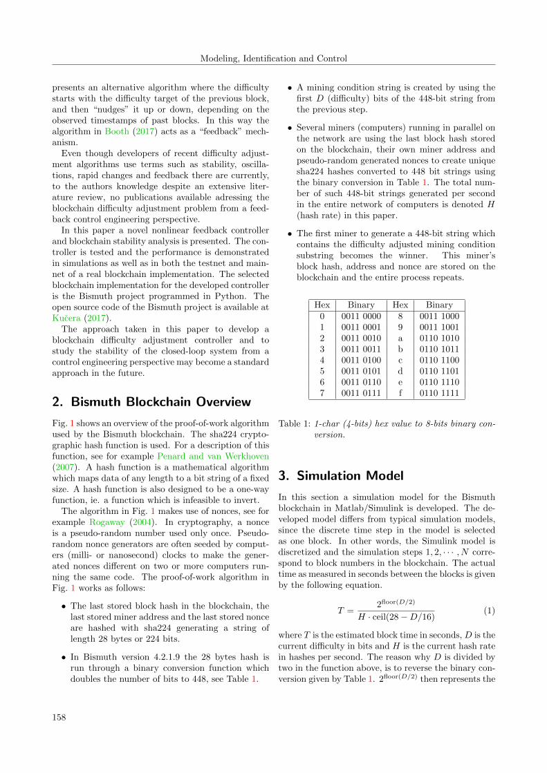
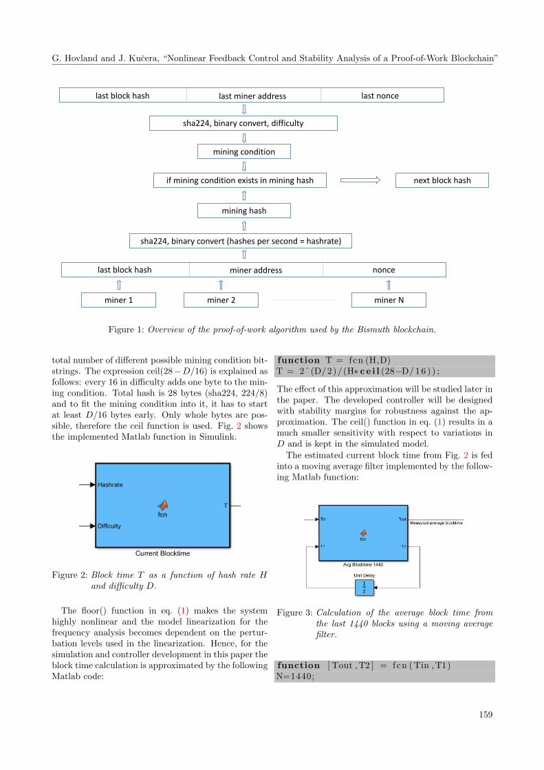
Fig. 1 shows an overview of the proof-of-work algorithmused by the Bismuth blockchain. The sha224 crypto-graphic hash function is used. For a description of thisfunction, see for example Penard and van Werkhoven(2007). A hash function is a mathematical algorithmwhich maps data of any length to a bit string of a fixedsize. A hash function is also designed to be a one-wayfunction, ie. a function which is infeasible to invert.

The algorithm in Fig. 1 makes use of nonces, see forexample Rogaway (2004). In cryptography, a nonceis a pseudo-random number used only once. Pseudo-random nonce generators are often seeded by comput-ers (milli- or nanosecond) clocks to make the gener-ated nonces different on two or more computers run-ning the same code. The proof-of-work algorithm inFig. 1 works as follows:

• The last stored block hash in the blockchain, thelast stored miner address and the last stored nonceare hashed with sha224 generating a string oflength 28 bytes or 224 bits.

• In Bismuth version 4.2.1.9 the 28 bytes hash isrun through a binary conversion function whichdoubles the number of bits to 448, see Table 1.

• A mining condition string is created by using thefirst D (difficulty) bits of the 448-bit string fromthe previous step.

• Several miners (computers) running in parallel onthe network are using the last block hash storedon the blockchain, their own miner address andpseudo-random generated nonces to create uniquesha224 hashes converted to 448 bit strings usingthe binary conversion in Table 1. The total num-ber of such 448-bit strings generated per secondin the entire network of computers is denoted H(hash rate) in this paper.

• The first miner to generate a 448-bit string whichcontains the difficulty adjusted mining conditionsubstring becomes the winner. This miner’sblock hash, address and nonce are stored on theblockchain and the entire process repeats.

Hex Binary Hex Binary0 0011 0000 8 0011 10001 0011 0001 9 0011 10012 0011 0010 a 0110 10103 0011 0011 b 0110 10114 0011 0100 c 0110 11005 0011 0101 d 0110 11016 0011 0110 e 0110 11107 0011 0111 f 0110 1111

Table 1: 1-char (4-bits) hex value to 8-bits binary con-version.

3. Simulation Model

In this section a simulation model for the Bismuthblockchain in Matlab/Simulink is developed. The de-veloped model differs from typical simulation models,since the discrete time step in the model is selectedas one block. In other words, the Simulink model isdiscretized and the simulation steps 1, 2, · · · , N corre-spond to block numbers in the blockchain. The actualtime as measured in seconds between the blocks is givenby the following equation.

T =2floor(D/2)

H · ceil(28−D/16)(1)

where T is the estimated block time in seconds, D is thecurrent difficulty in bits and H is the current hash ratein hashes per second. The reason why D is divided bytwo in the function above, is to reverse the binary con-version given by Table 1. 2floor(D/2) then represents the

158

G. Hovland and J. Kucera, “Nonlinear Feedback Control and Stability Analysis of a Proof-of-Work Blockchain”

last noncelast block hash last miner address

sha224, binary convert, difficulty

miner 1

noncelast block hash miner address

mining condition

miner 2 miner N

sha224, binary convert (hashes per second = hashrate)

if mining condition exists in mining hash

mining hash

next block hash

Figure 1: Overview of the proof-of-work algorithm used by the Bismuth blockchain.

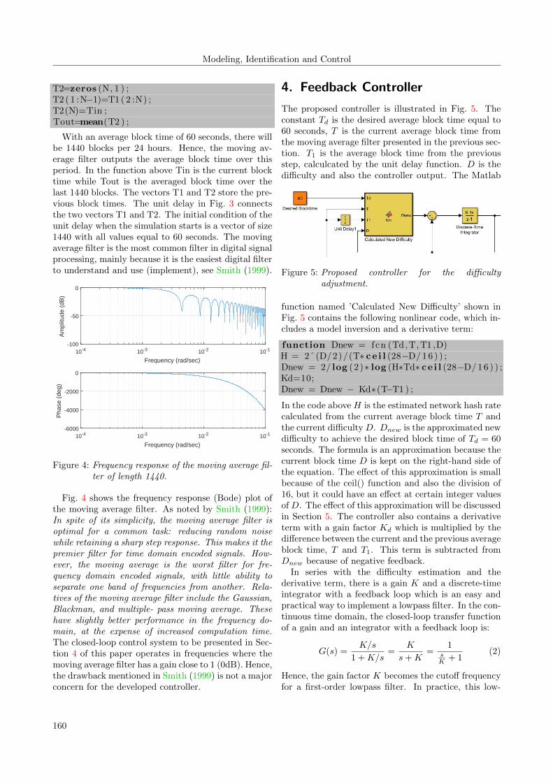
total number of different possible mining condition bit-strings. The expression ceil(28−D/16) is explained asfollows: every 16 in difficulty adds one byte to the min-ing condition. Total hash is 28 bytes (sha224, 224/8)and to fit the mining condition into it, it has to startat least D/16 bytes early. Only whole bytes are pos-sible, therefore the ceil function is used. Fig. 2 showsthe implemented Matlab function in Simulink.

Figure 2: Block time T as a function of hash rate Hand difficulty D.

The floor() function in eq. (1) makes the systemhighly nonlinear and the model linearization for thefrequency analysis becomes dependent on the pertur-bation levels used in the linearization. Hence, for thesimulation and controller development in this paper theblock time calculation is approximated by the followingMatlab code:

function T = fcn (H,D)T = 2ˆ(D/2)/(H∗ ce i l (28−D/ 1 6 ) ) ;

The effect of this approximation will be studied later inthe paper. The developed controller will be designedwith stability margins for robustness against the ap-proximation. The ceil() function in eq. (1) results in amuch smaller sensitivity with respect to variations inD and is kept in the simulated model.

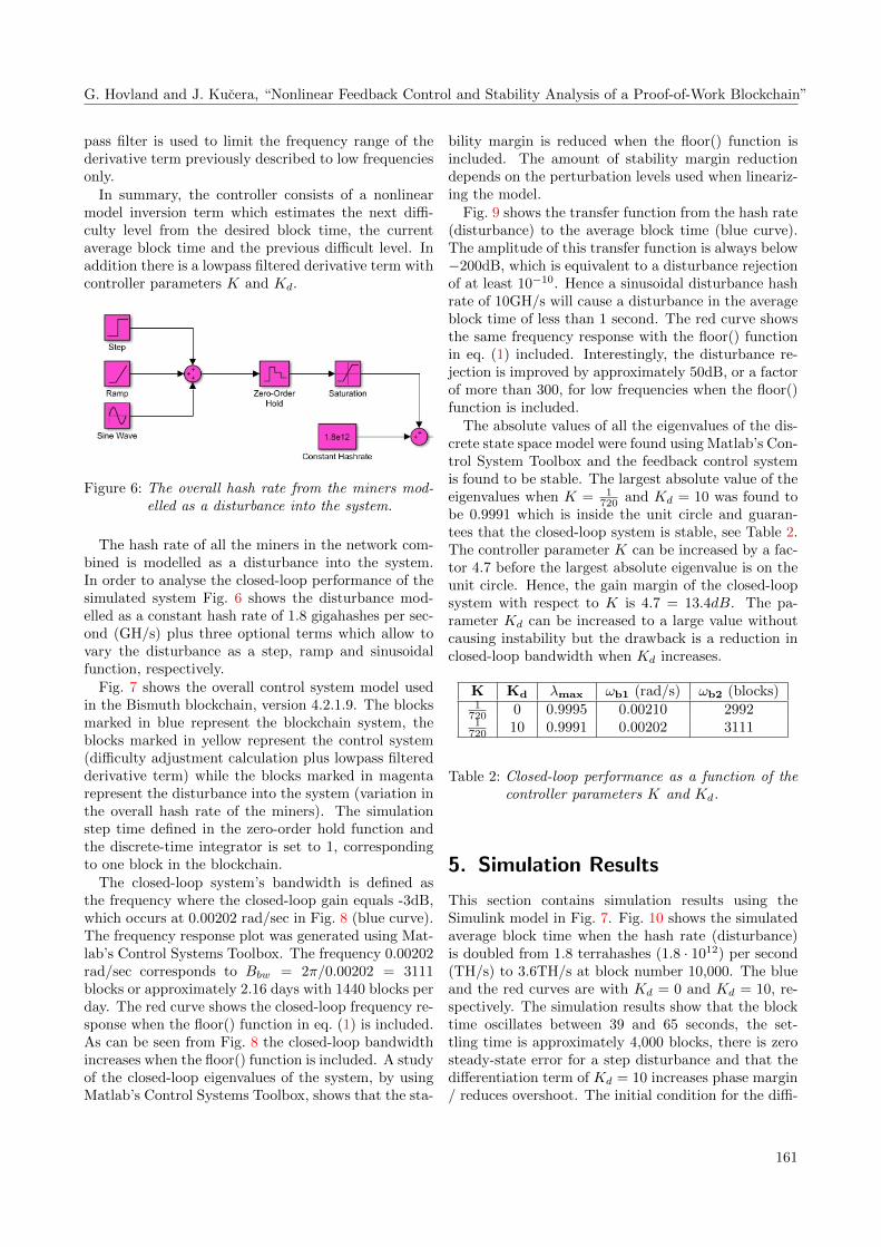
The estimated current block time from Fig. 2 is fedinto a moving average filter implemented by the follow-ing Matlab function:

Figure 3: Calculation of the average block time fromthe last 1440 blocks using a moving averagefilter.

function [ Tout , T2 ] = fcn ( Tin , T1)N=1440;

159

Modeling, Identification and Control

T2=zeros (N, 1 ) ;T2 ( 1 :N−1)=T1 ( 2 :N) ;T2(N)=Tin ;Tout=mean(T2 ) ;

With an average block time of 60 seconds, there willbe 1440 blocks per 24 hours. Hence, the moving av-erage filter outputs the average block time over thisperiod. In the function above Tin is the current blocktime while Tout is the averaged block time over thelast 1440 blocks. The vectors T1 and T2 store the pre-vious block times. The unit delay in Fig. 3 connectsthe two vectors T1 and T2. The initial condition of theunit delay when the simulation starts is a vector of size1440 with all values equal to 60 seconds. The movingaverage filter is the most common filter in digital signalprocessing, mainly because it is the easiest digital filterto understand and use (implement), see Smith (1999).

10-4 10-3 10-2 10-1

Frequency (rad/sec)

-100

-50

0

Am

plitu

de (

dB)

10-4 10-3 10-2 10-1

Frequency (rad/sec)

-6000

-4000

-2000

0

Pha

se (

deg)

Figure 4: Frequency response of the moving average fil-ter of length 1440.

Fig. 4 shows the frequency response (Bode) plot ofthe moving average filter. As noted by Smith (1999):In spite of its simplicity, the moving average filter isoptimal for a common task: reducing random noisewhile retaining a sharp step response. This makes it thepremier filter for time domain encoded signals. How-ever, the moving average is the worst filter for fre-quency domain encoded signals, with little ability toseparate one band of frequencies from another. Rela-tives of the moving average filter include the Gaussian,Blackman, and multiple- pass moving average. Thesehave slightly better performance in the frequency do-main, at the expense of increased computation time.The closed-loop control system to be presented in Sec-tion 4 of this paper operates in frequencies where themoving average filter has a gain close to 1 (0dB). Hence,the drawback mentioned in Smith (1999) is not a majorconcern for the developed controller.

4. Feedback Controller

The proposed controller is illustrated in Fig. 5. Theconstant Td is the desired average block time equal to60 seconds, T is the current average block time fromthe moving average filter presented in the previous sec-tion. T1 is the average block time from the previousstep, calculcated by the unit delay function. D is thedifficulty and also the controller output. The Matlab

Figure 5: Proposed controller for the difficultyadjustment.

function named ’Calculated New Difficulty’ shown inFig. 5 contains the following nonlinear code, which in-cludes a model inversion and a derivative term:

function Dnew = fcn (Td,T, T1 ,D)H = 2ˆ(D/2)/(T∗ ce i l (28−D/ 1 6 ) ) ;Dnew = 2/ log (2)∗ log (H∗Td∗ ce i l (28−D/ 1 6 ) ) ;Kd=10;Dnew = Dnew − Kd∗(T−T1 ) ;

In the code above H is the estimated network hash ratecalculated from the current average block time T andthe current difficulty D. Dnew is the approximated newdifficulty to achieve the desired block time of Td = 60seconds. The formula is an approximation because thecurrent block time D is kept on the right-hand side ofthe equation. The effect of this approximation is smallbecause of the ceil() function and also the division of16, but it could have an effect at certain integer valuesof D. The effect of this approximation will be discussedin Section 5. The controller also contains a derivativeterm with a gain factor Kd which is multiplied by thedifference between the current and the previous averageblock time, T and T1. This term is subtracted fromDnew because of negative feedback.

In series with the difficulty estimation and thederivative term, there is a gain K and a discrete-timeintegrator with a feedback loop which is an easy andpractical way to implement a lowpass filter. In the con-tinuous time domain, the closed-loop transfer functionof a gain and an integrator with a feedback loop is:

G(s) =K/s

1 +K/s=

K

s+K=

1sK + 1

(2)

Hence, the gain factor K becomes the cutoff frequencyfor a first-order lowpass filter. In practice, this low-

160

G. Hovland and J. Kucera, “Nonlinear Feedback Control and Stability Analysis of a Proof-of-Work Blockchain”

pass filter is used to limit the frequency range of thederivative term previously described to low frequenciesonly.

In summary, the controller consists of a nonlinearmodel inversion term which estimates the next diffi-culty level from the desired block time, the currentaverage block time and the previous difficult level. Inaddition there is a lowpass filtered derivative term withcontroller parameters K and Kd.

Figure 6: The overall hash rate from the miners mod-elled as a disturbance into the system.

The hash rate of all the miners in the network com-bined is modelled as a disturbance into the system.In order to analyse the closed-loop performance of thesimulated system Fig. 6 shows the disturbance mod-elled as a constant hash rate of 1.8 gigahashes per sec-ond (GH/s) plus three optional terms which allow tovary the disturbance as a step, ramp and sinusoidalfunction, respectively.

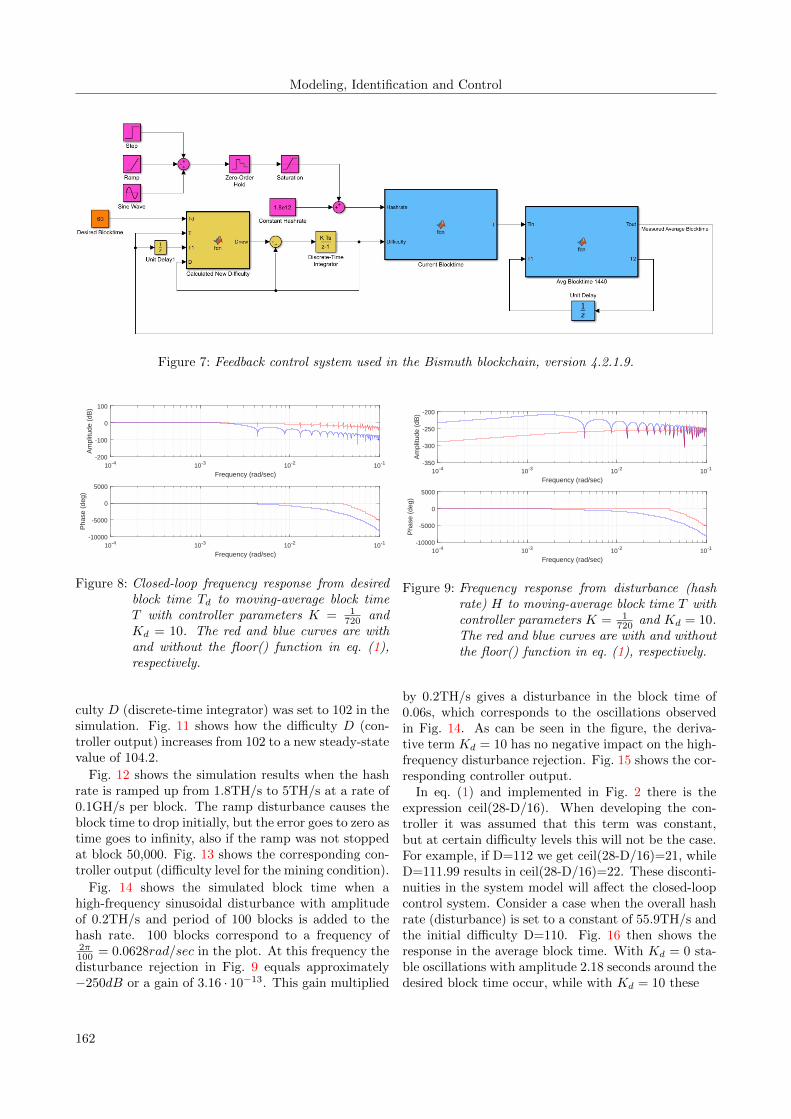
Fig. 7 shows the overall control system model usedin the Bismuth blockchain, version 4.2.1.9. The blocksmarked in blue represent the blockchain system, theblocks marked in yellow represent the control system(difficulty adjustment calculation plus lowpass filteredderivative term) while the blocks marked in magentarepresent the disturbance into the system (variation inthe overall hash rate of the miners). The simulationstep time defined in the zero-order hold function andthe discrete-time integrator is set to 1, correspondingto one block in the blockchain.

The closed-loop system’s bandwidth is defined asthe frequency where the closed-loop gain equals -3dB,which occurs at 0.00202 rad/sec in Fig. 8 (blue curve).The frequency response plot was generated using Mat-lab’s Control Systems Toolbox. The frequency 0.00202rad/sec corresponds to Bbw = 2π/0.00202 = 3111blocks or approximately 2.16 days with 1440 blocks perday. The red curve shows the closed-loop frequency re-sponse when the floor() function in eq. (1) is included.As can be seen from Fig. 8 the closed-loop bandwidthincreases when the floor() function is included. A studyof the closed-loop eigenvalues of the system, by usingMatlab’s Control Systems Toolbox, shows that the sta-

bility margin is reduced when the floor() function isincluded. The amount of stability margin reductiondepends on the perturbation levels used when lineariz-ing the model.

Fig. 9 shows the transfer function from the hash rate(disturbance) to the average block time (blue curve).The amplitude of this transfer function is always below−200dB, which is equivalent to a disturbance rejectionof at least 10−10. Hence a sinusoidal disturbance hashrate of 10GH/s will cause a disturbance in the averageblock time of less than 1 second. The red curve showsthe same frequency response with the floor() functionin eq. (1) included. Interestingly, the disturbance re-jection is improved by approximately 50dB, or a factorof more than 300, for low frequencies when the floor()function is included.

The absolute values of all the eigenvalues of the dis-crete state space model were found using Matlab’s Con-trol System Toolbox and the feedback control systemis found to be stable. The largest absolute value of theeigenvalues when K = 1

720 and Kd = 10 was found tobe 0.9991 which is inside the unit circle and guaran-tees that the closed-loop system is stable, see Table 2.The controller parameter K can be increased by a fac-tor 4.7 before the largest absolute eigenvalue is on theunit circle. Hence, the gain margin of the closed-loopsystem with respect to K is 4.7 = 13.4dB. The pa-rameter Kd can be increased to a large value withoutcausing instability but the drawback is a reduction inclosed-loop bandwidth when Kd increases.

K Kd λmax ωb1 (rad/s) ωb2 (blocks)1

720 0 0.9995 0.00210 29921

720 10 0.9991 0.00202 3111

Table 2: Closed-loop performance as a function of thecontroller parameters K and Kd.

5. Simulation Results

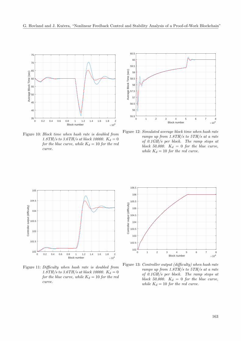
This section contains simulation results using theSimulink model in Fig. 7. Fig. 10 shows the simulatedaverage block time when the hash rate (disturbance)is doubled from 1.8 terrahashes (1.8 · 1012) per second(TH/s) to 3.6TH/s at block number 10,000. The blueand the red curves are with Kd = 0 and Kd = 10, re-spectively. The simulation results show that the blocktime oscillates between 39 and 65 seconds, the set-tling time is approximately 4,000 blocks, there is zerosteady-state error for a step disturbance and that thedifferentiation term of Kd = 10 increases phase margin/ reduces overshoot. The initial condition for the diffi-

161

Modeling, Identification and Control

Figure 7: Feedback control system used in the Bismuth blockchain, version 4.2.1.9.

10-4 10-3 10-2 10-1

Frequency (rad/sec)

-200

-100

0

100

Am

plitu

de (

dB)

10-4 10-3 10-2 10-1

Frequency (rad/sec)

-10000

-5000

0

5000

Pha

se (

deg)

Figure 8: Closed-loop frequency response from desiredblock time Td to moving-average block timeT with controller parameters K = 1

720 andKd = 10. The red and blue curves are withand without the floor() function in eq. (1),respectively.

culty D (discrete-time integrator) was set to 102 in thesimulation. Fig. 11 shows how the difficulty D (con-troller output) increases from 102 to a new steady-statevalue of 104.2.

Fig. 12 shows the simulation results when the hashrate is ramped up from 1.8TH/s to 5TH/s at a rate of0.1GH/s per block. The ramp disturbance causes theblock time to drop initially, but the error goes to zero astime goes to infinity, also if the ramp was not stoppedat block 50,000. Fig. 13 shows the corresponding con-troller output (difficulty level for the mining condition).

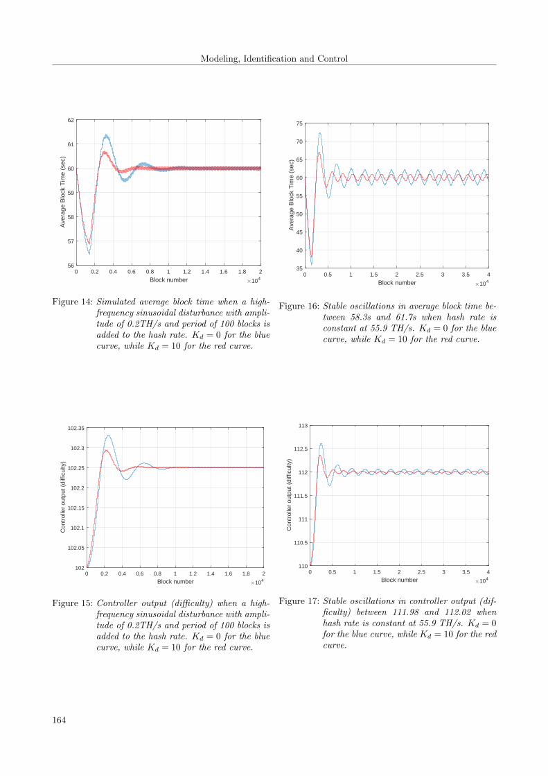
Fig. 14 shows the simulated block time when ahigh-frequency sinusoidal disturbance with amplitudeof 0.2TH/s and period of 100 blocks is added to thehash rate. 100 blocks correspond to a frequency of2π100 = 0.0628rad/sec in the plot. At this frequency thedisturbance rejection in Fig. 9 equals approximately−250dB or a gain of 3.16 · 10−13. This gain multiplied

10-4 10-3 10-2 10-1

Frequency (rad/sec)

-350

-300

-250

-200A

mpl

itude

(dB

)

10-4 10-3 10-2 10-1

Frequency (rad/sec)

-10000

-5000

0

5000

Pha

se (

deg)

Figure 9: Frequency response from disturbance (hashrate) H to moving-average block time T withcontroller parameters K = 1

720 and Kd = 10.The red and blue curves are with and withoutthe floor() function in eq. (1), respectively.

by 0.2TH/s gives a disturbance in the block time of0.06s, which corresponds to the oscillations observedin Fig. 14. As can be seen in the figure, the deriva-tive term Kd = 10 has no negative impact on the high-frequency disturbance rejection. Fig. 15 shows the cor-responding controller output.

In eq. (1) and implemented in Fig. 2 there is theexpression ceil(28-D/16). When developing the con-troller it was assumed that this term was constant,but at certain difficulty levels this will not be the case.For example, if D=112 we get ceil(28-D/16)=21, whileD=111.99 results in ceil(28-D/16)=22. These disconti-nuities in the system model will affect the closed-loopcontrol system. Consider a case when the overall hashrate (disturbance) is set to a constant of 55.9TH/s andthe initial difficulty D=110. Fig. 16 then shows theresponse in the average block time. With Kd = 0 sta-ble oscillations with amplitude 2.18 seconds around thedesired block time occur, while with Kd = 10 these

162

G. Hovland and J. Kucera, “Nonlinear Feedback Control and Stability Analysis of a Proof-of-Work Blockchain”

0 0.2 0.4 0.6 0.8 1 1.2 1.4 1.6 1.8 2

Block number 104

35

40

45

50

55

60

65

70

75

Ave

rage

Blo

ck T

ime

(sec

)

Figure 10: Block time when hash rate is doubled from1.8TH/s to 3.6TH/s at block 10000. Kd = 0for the blue curve, while Kd = 10 for the redcurve.

0 0.2 0.4 0.6 0.8 1 1.2 1.4 1.6 1.8 2

Block number 104

102

102.5

103

103.5

104

104.5

105

Con

trol

ler

outp

ut (

diffi

culty

)

Figure 11: Difficulty when hash rate is doubled from1.8TH/s to 3.6TH/s at block 10000. Kd = 0for the blue curve, while Kd = 10 for the redcurve.

0 1 2 3 4 5 6 7 8

Block number 104

55.5

56

56.5

57

57.5

58

58.5

59

59.5

60

60.5

Ave

rage

Blo

ck T

ime

(sec

)

Figure 12: Simulated average block time when hash rateramps up from 1.8TH/s to 5TH/s at a rateof 0.1GH/s per block. The ramp stops atblock 50,000. Kd = 0 for the blue curve,while Kd = 10 for the red curve.

0 1 2 3 4 5 6 7 8

Block number 104

102

102.5

103

103.5

104

104.5

105

105.5

106

106.5

Con

trol

ler

outp

ut (

diffi

culty

)

Figure 13: Controller output (difficulty) when hash rateramps up from 1.8TH/s to 5TH/s at a rateof 0.1GH/s per block. The ramp stops atblock 50,000. Kd = 0 for the blue curve,while Kd = 10 for the red curve.

163

Modeling, Identification and Control

0 0.2 0.4 0.6 0.8 1 1.2 1.4 1.6 1.8 2

Block number 104

56

57

58

59

60

61

62

Ave

rage

Blo

ck T

ime

(sec

)

Figure 14: Simulated average block time when a high-frequency sinusoidal disturbance with ampli-tude of 0.2TH/s and period of 100 blocks isadded to the hash rate. Kd = 0 for the bluecurve, while Kd = 10 for the red curve.

0 0.2 0.4 0.6 0.8 1 1.2 1.4 1.6 1.8 2

Block number 104

102

102.05

102.1

102.15

102.2

102.25

102.3

102.35

Con

trol

ler

outp

ut (

diffi

culty

)

Figure 15: Controller output (difficulty) when a high-frequency sinusoidal disturbance with ampli-tude of 0.2TH/s and period of 100 blocks isadded to the hash rate. Kd = 0 for the bluecurve, while Kd = 10 for the red curve.

0 0.5 1 1.5 2 2.5 3 3.5 4

Block number 104

35

40

45

50

55

60

65

70

75

Ave

rage

Blo

ck T

ime

(sec

)

Figure 16: Stable oscillations in average block time be-tween 58.3s and 61.7s when hash rate isconstant at 55.9 TH/s. Kd = 0 for the bluecurve, while Kd = 10 for the red curve.

0 0.5 1 1.5 2 2.5 3 3.5 4

Block number 104

110

110.5

111

111.5

112

112.5

113

Con

trol

ler

outp

ut (

diffi

culty

)

Figure 17: Stable oscillations in controller output (dif-ficulty) between 111.98 and 112.02 whenhash rate is constant at 55.9 TH/s. Kd = 0for the blue curve, while Kd = 10 for the redcurve.

164

G. Hovland and J. Kucera, “Nonlinear Feedback Control and Stability Analysis of a Proof-of-Work Blockchain”

oscillcations are reduced to an amplitude of 0.81 sec-onds. In other words, the derivative term Kd increasesthe damping in the closed-loop system and reducesthe oscillation in this particular case by a factor 2.7.Fig. 17 shows the corresponding controller output (dif-ficulty) as it initially starts at 110 and goes towards112. The stable oscillations in the controller outputare caused by the discontinuous ceil() function in thesystem model. This behaviour of the closed-loop sys-tem will occur at the following discrete set of difficultylevels D ∈ {8, 16, 24, · · · , 432}.

6. Blockchain Network Results

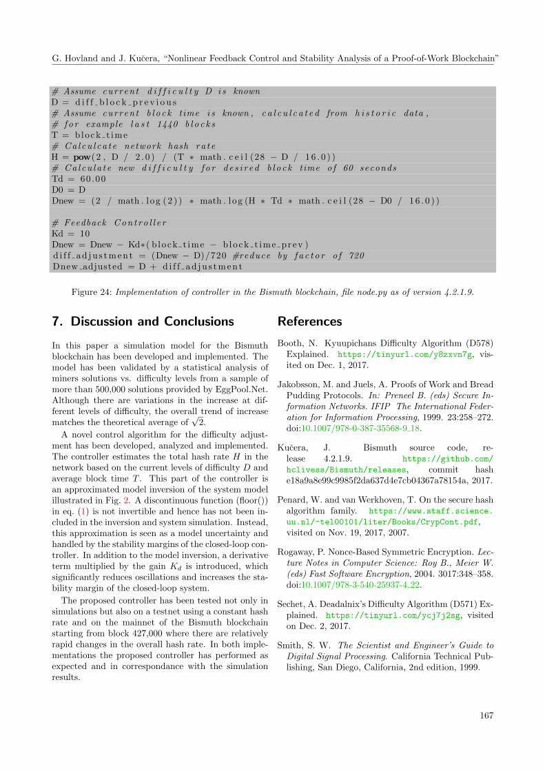
In addition to simulations the difficulty adjustmentfeedback controller developed in this paper is imple-mented in the Bismuth blockchain as of version 4.2.1.9.The code in Fig. 24 shows the actual code implementedin Python.

0 1000 2000 3000 4000 5000 6000 7000 8000 9000 10000

Block number

40

50

60

70

80

90

100

110

Blo

ck ti

me

(sec

)

Bismuth 4.1.9 Testnet, Constant Hash rate

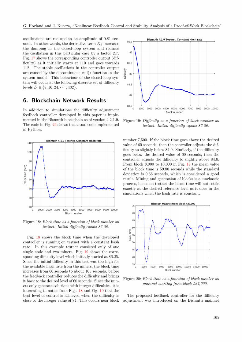
Figure 18: Block time as a function of block number ontestnet. Initial difficulty equals 86.26.

Fig. 18 shows the block time when the developedcontroller is running on testnet with a constant hashrate. In this example testnet consisted only of onesingle node and two miners. Fig. 19 shows the corre-sponding difficulty level which initially started at 86.25.Since the initial difficulty in this test was too high forthe available hash rate from the miners, the block timeincreases from 60 seconds to about 105 seconds, beforethe feedback controller reduces the difficulty and bringsit back to the desired level of 60 seconds. Since the min-ers only generate solutions with integer difficulties, it isinteresting to notice from Figs. 18 and Fig. 19 that thebest level of control is achieved when the difficulty isclose to the integer value of 84. This occurs near block

0 1000 2000 3000 4000 5000 6000 7000 8000 9000 10000

Block number

83.5

84

84.5

85

85.5

86

86.5

Diff

icul

ty

Bismuth 4.1.9 Testnet, Constant Hash rate

Figure 19: Difficulty as a function of block number ontestnet. Initial difficulty equals 86.26.

number 7,500. If the block time goes above the desiredvalue of 60 seconds, then the controller adjusts the dif-ficulty to slightly below 84.0. Similarly, if the difficultygoes below the desired value of 60 seconds, then thecontroller adjusts the difficulty to slightly above 84.0.From block 8,000 to 10,000 in Fig. 18 the mean valueof the block time is 59.80 seconds while the standarddeviation is 0.66 seconds, which is considered a goodresult. Mining and generation of blocks is a stochasticprocess, hence on testnet the block time will not settleexactly at the desired reference level as it does in thesimulations when the hash rate is constant.

0 2000 4000 6000 8000 10000 12000 14000 16000

Block number

35

40

45

50

55

60

65

70

75

Blo

ck T

ime

Bismuth Mainnet from Block 427,000

Figure 20: Block time as a function of block number onmainnet starting from block 427,000.

The proposed feedback controller for the difficultyadjustment was introduced on the Bismuth mainnet

165

Modeling, Identification and Control

0 2000 4000 6000 8000 10000 12000 14000 16000

Block number

102.5

103

103.5

104

104.5

105

105.5

106

106.5

Diff

icul

ty

Bismuth Mainnet from Block 427,000

Figure 21: Difficulty as a function of block number onmainnet starting from block 427,000.

0 2000 4000 6000 8000 10000 12000 14000 16000

Block number

2000

3000

4000

5000

6000

7000

8000

Has

h ra

te (

GH

/s)

Bismuth Mainnet from Block 427,000

Figure 22: Hash rate as a function of block number onmainnet starting from block 427,000.

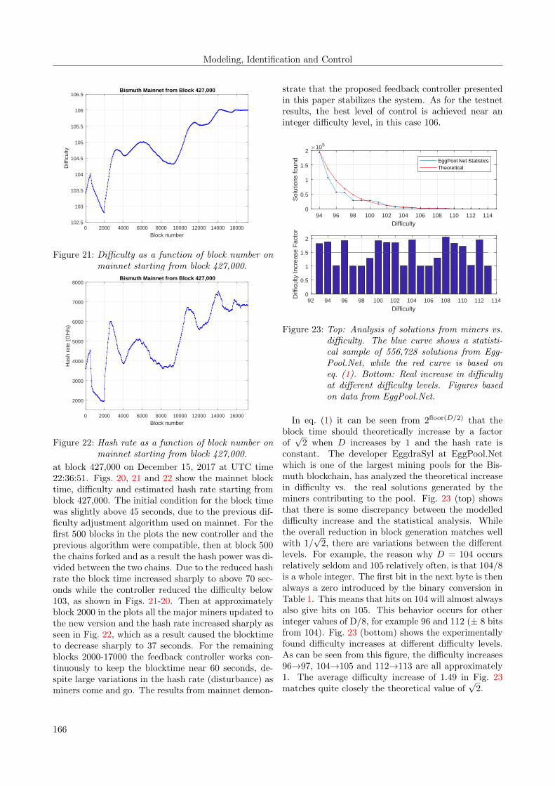
at block 427,000 on December 15, 2017 at UTC time22:36:51. Figs. 20, 21 and 22 show the mainnet blocktime, difficulty and estimated hash rate starting fromblock 427,000. The initial condition for the block timewas slightly above 45 seconds, due to the previous dif-ficulty adjustment algorithm used on mainnet. For thefirst 500 blocks in the plots the new controller and theprevious algorithm were compatible, then at block 500the chains forked and as a result the hash power was di-vided between the two chains. Due to the reduced hashrate the block time increased sharply to above 70 sec-onds while the controller reduced the difficulty below103, as shown in Figs. 21-20. Then at approximatelyblock 2000 in the plots all the major miners updated tothe new version and the hash rate increased sharply asseen in Fig. 22, which as a result caused the blocktimeto decrease sharply to 37 seconds. For the remainingblocks 2000-17000 the feedback controller works con-tinuously to keep the blocktime near 60 seconds, de-spite large variations in the hash rate (disturbance) asminers come and go. The results from mainnet demon-

strate that the proposed feedback controller presentedin this paper stabilizes the system. As for the testnetresults, the best level of control is achieved near aninteger difficulty level, in this case 106.

94 96 98 100 102 104 106 108 110 112 114

Difficulty

0

0.5

1

1.5

2

Sol

utio

ns fo

und

105

EggPool.Net StatisticsTheoretical

92 94 96 98 100 102 104 106 108 110 112 114

Difficulty

0

0.5

1

1.5

2

Diff

icul

ty In

crea

se F

acto

r

Figure 23: Top: Analysis of solutions from miners vs.difficulty. The blue curve shows a statisti-cal sample of 556,728 solutions from Egg-Pool.Net, while the red curve is based oneq. (1). Bottom: Real increase in difficultyat different difficulty levels. Figures basedon data from EggPool.Net.

In eq. (1) it can be seen from 2floor(D/2) that theblock time should theoretically increase by a factorof√

2 when D increases by 1 and the hash rate isconstant. The developer EggdraSyl at EggPool.Netwhich is one of the largest mining pools for the Bis-muth blockchain, has analyzed the theoretical increasein difficulty vs. the real solutions generated by theminers contributing to the pool. Fig. 23 (top) showsthat there is some discrepancy between the modelleddifficulty increase and the statistical analysis. Whilethe overall reduction in block generation matches wellwith 1/

√2, there are variations between the different

levels. For example, the reason why D = 104 occursrelatively seldom and 105 relatively often, is that 104/8is a whole integer. The first bit in the next byte is thenalways a zero introduced by the binary conversion inTable 1. This means that hits on 104 will almost alwaysalso give hits on 105. This behavior occurs for otherinteger values of D/8, for example 96 and 112 (± 8 bitsfrom 104). Fig. 23 (bottom) shows the experimentallyfound difficulty increases at different difficulty levels.As can be seen from this figure, the difficulty increases96→97, 104→105 and 112→113 are all approximately1. The average difficulty increase of 1.49 in Fig. 23matches quite closely the theoretical value of

√2.

166

G. Hovland and J. Kucera, “Nonlinear Feedback Control and Stability Analysis of a Proof-of-Work Blockchain”

# Assume current d i f f i c u l t y D i s knownD = d i f f b l o c k p r e v i o u s# Assume current b l o c k time i s known , c a l c u l c a t e d from h i s t o r i c data ,# f o r example l a s t 1440 b l o c k sT = block t ime# C a l c u l c a t e network hash r a t eH = pow(2 , D / 2 . 0 ) / (T ∗ math . c e i l (28 − D / 1 6 . 0 ) )# C a l c u l a t e new d i f f i c u l t y f o r d e s i r e d b l o c k time o f 60 secondsTd = 60.00D0 = DDnew = (2 / math . l og ( 2 ) ) ∗ math . l og (H ∗ Td ∗ math . c e i l (28 − D0 / 1 6 . 0 ) )

# Feedback C o n t r o l l e rKd = 10Dnew = Dnew − Kd∗( b lock t ime − b lock t ime prev )d i f f a d j u s t m e n t = (Dnew − D)/720 #reduce by f a c t o r o f 720Dnew adjusted = D + d i f f a d j u s t m e n t

Figure 24: Implementation of controller in the Bismuth blockchain, file node.py as of version 4.2.1.9.

7. Discussion and Conclusions

In this paper a simulation model for the Bismuthblockchain has been developed and implemented. Themodel has been validated by a statistical analysis ofminers solutions vs. difficulty levels from a sample ofmore than 500,000 solutions provided by EggPool.Net.Although there are variations in the increase at dif-ferent levels of difficulty, the overall trend of increasematches the theoretical average of

√2.

A novel control algorithm for the difficulty adjust-ment has been developed, analyzed and implemented.The controller estimates the total hash rate H in thenetwork based on the current levels of difficulty D andaverage block time T . This part of the controller isan approximated model inversion of the system modelillustrated in Fig. 2. A discontinuous function (floor())in eq. (1) is not invertible and hence has not been in-cluded in the inversion and system simulation. Instead,this approximation is seen as a model uncertainty andhandled by the stability margins of the closed-loop con-troller. In addition to the model inversion, a derivativeterm multiplied by the gain Kd is introduced, whichsignificantly reduces oscillations and increases the sta-bility margin of the closed-loop system.

The proposed controller has been tested not only insimulations but also on a testnet using a constant hashrate and on the mainnet of the Bismuth blockchainstarting from block 427,000 where there are relativelyrapid changes in the overall hash rate. In both imple-mentations the proposed controller has performed asexpected and in correspondance with the simulationresults.

References

Booth, N. Kyuupichans Difficulty Algorithm (D578)Explained. https://tinyurl.com/y8zxvn7g, vis-ited on Dec. 1, 2017.

Jakobsson, M. and Juels, A. Proofs of Work and BreadPudding Protocols. In: Preneel B. (eds) Secure In-formation Networks. IFIP The International Feder-ation for Information Processing, 1999. 23:258–272.doi:10.1007/978-0-387-35568-9 18.

Kucera, J. Bismuth source code, re-lease 4.2.1.9. https://github.com/

hclivess/Bismuth/releases, commit hashe18a9a8e99c9985f2da637d4e7cb04367a78154a, 2017.

Penard, W. and van Werkhoven, T. On the secure hashalgorithm family. https://www.staff.science.

uu.nl/~tel00101/liter/Books/CrypCont.pdf,visited on Nov. 19, 2017, 2007.

Rogaway, P. Nonce-Based Symmetric Encryption. Lec-ture Notes in Computer Science: Roy B., Meier W.(eds) Fast Software Encryption, 2004. 3017:348–358.doi:10.1007/978-3-540-25937-4 22.

Sechet, A. Deadalnix’s Difficulty Algorithm (D571) Ex-plained. https://tinyurl.com/ycj7j2sg, visitedon Dec. 2, 2017.

Smith, S. W. The Scientist and Engineer’s Guide toDigital Signal Processing. California Technical Pub-lishing, San Diego, California, 2nd edition, 1999.

167

Modeling, Identification and Control

import j son , base64 , hash l ib , socks , connec t i ons

def f i l e h a s h ( f i l ename ) :#f i l e h a s hh = hash l i b . sha256 ( )with open( f i l ename , ’ rb ’ , b u f f e r i n g =0) as f :

for b in iter (lambda : f . read (128∗1024) , b ’ ’ ) :h . update (b)

return h . hexd ige s t ( )#f i l e h a s h

def b lockge t ( socket , arg1 ) :#g e t b l o c kconnec t i ons . send ( s , ” b lockge t ” , 10)connec t i ons . send ( s , arg1 , 10)b l o c k g e t = connect ions . r e c e i v e ( s , 10)return b l o c k g e t#g e t b l o c k

s = socks . socksocke t ( )s . s e t t imeout (10)s . connect ( ( ” 1 2 7 . 0 . 0 . 1 ” , 5658))b lock = blockge t ( s , 406054)s . c l o s e ( )

jsonData = block [ 0 ] [ 1 1 ] [ 4 : ]jsonToPython = json . l oads ( jsonData )

with open( jsonToPython [ ’ f i l ename ’ ] , ”wb” ) as fh :fh . wr i t e ( base64 . b64decode ( jsonToPython [ ’ data ’ ] . encode ( ’ a s c i i ’ ) ) )

f i l e h a s h = f i l e h a s h ( jsonToPython [ ’ f i l ename ’ ] )print ( ” F i l e {} ex t rac t ed ” . format ( jsonToPython [ ’ f i l ename ’ ] ) )print ( ” F i l e hash matches : {}” . format ( f i l e h a s h == jsonToPython [ ’ sha256 ’ ] ) )

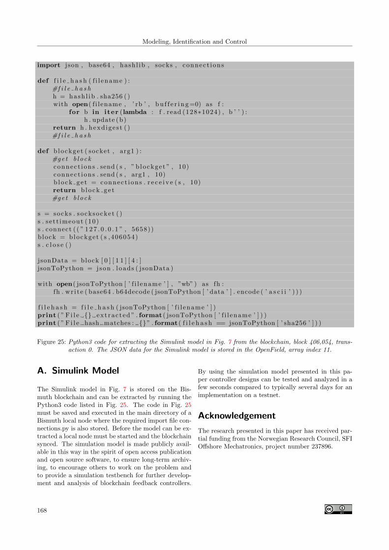
Figure 25: Python3 code for extracting the Simulink model in Fig. 7 from the blockchain, block 406,054, trans-action 0. The JSON data for the Simulink model is stored in the OpenField, array index 11.

A. Simulink Model

The Simulink model in Fig. 7 is stored on the Bis-muth blockchain and can be extracted by running thePython3 code listed in Fig. 25. The code in Fig. 25must be saved and executed in the main directory of aBismuth local node where the required import file con-nections.py is also stored. Before the model can be ex-tracted a local node must be started and the blockchainsynced. The simulation model is made publicly avail-able in this way in the spirit of open access publicationand open source software, to ensure long-term archiv-ing, to encourage others to work on the problem andto provide a simulation testbench for further develop-ment and analysis of blockchain feedback controllers.

By using the simulation model presented in this pa-per controller designs can be tested and analyzed in afew seconds compared to typically several days for animplementation on a testnet.

Acknowledgement

The research presented in this paper has received par-tial funding from the Norwegian Research Council, SFIOffshore Mechatronics, project number 237896.

168