Nonrigid Structure-from-Motion: Estimating Shape and Motion with Hierarchical Priors

Nonrigid Structure-from-Motion: EstimatingShape and Motion with Hierarchical Priors

Lorenzo Torresani, Aaron Hertzmann, Member, IEEE, and Christoph Bregler

Abstract—This paper describes methods for recovering time-varying shape and motion of nonrigid 3D objects from uncalibrated

2D point tracks. For example, given a video recording of a talking person, we would like to estimate the 3D shape of the face at each

instant and learn a model of facial deformation. Time-varying shape is modeled as a rigid transformation combined with a nonrigid

deformation. Reconstruction is ill-posed if arbitrary deformations are allowed, and thus additional assumptions about deformations are

required. We first suggest restricting shapes to lie within a low-dimensional subspace and describe estimation algorithms. However, this

restriction alone is insufficient to constrain reconstruction. To address these problems, we propose a reconstruction method using a

Probabilistic Principal Components Analysis (PPCA) shape model and an estimation algorithm that simultaneously estimates 3D shape

and motion for each instant, learns the PPCA model parameters, and robustly fills-in missing data points. We then extend the model to

represent temporal dynamics in object shape, allowing the algorithm to robustly handle severe cases of missing data.

Index Terms—Nonrigid structure-from-motion, probabilistic principal components analysis, factor analysis, linear dynamical systems,

expectation-maximization.

Ç

1 INTRODUCTION AND RELATED WORK

A central goal of computer vision is to reconstruct theshape and motion of objects from images. Reconstruc-

tion of shape and motion from point tracks—known asstructure-from-motion—is very well understood for rigidobjects [17], [26] and multiple rigid objects [10], [16].However, many objects in the real world deform over time,including people, animals, and elastic objects. Reconstructingthe shape of such objects from imagery remains an openproblem.

In this paper, we describe methods for NonrigidStructure-From-Motion (NRSFM): extracting 3D shape andmotion of nonrigid objects from 2D point tracks. Estimatingtime-varying 3D shape from monocular 2D point tracks isinherently underconstrained without prior assumptions.However, the apparent ease with which humans interpret3D motion from ambiguous point tracks (for example, [18],[30]) suggests that we might take advantage of priorassumptions about motion. A key question is what shouldthese prior assumptions be? One possible approach is toexplicitly describe which shapes are most likely (forexample, by hard-coding a model [32]), but this can beextremely difficult for all but the simplest cases. Anotherapproach is to learn a model from training data. Variousauthors have described methods for learning linear sub-space models with Principal Components Analysis (PCA)

for recognition, tracking, and reconstruction [4], [9], [24],[31]. This approach works well if appropriate training datais available; however, this is often not the case. In thispaper, we do not assume that any training data is available.

In this work, we model 3D shapes as lying near a low-dimensional subspace, with a Gaussian prior on each shapein the subspace. Additionally, we assume that the nonrigidobject undergoes a rigid transformation at each time instant(equivalently, a rigid camera motion), followed by a weak-perspective camera projection. This model is a form ofProbabilistic Principal Components Analysis (PPCA). A keyfeature of this approach is that we do not require any prior3D training data. Instead, the PPCA model is used as ahierarchical Bayesian prior [13] for the measurements. Thehierarchical prior makes it possible to simultaneouslyestimate the 3D shape and motion for all time instants,learn the deformation model, and robustly fill-in missingdata points. During estimation, we marginalize out defor-mation coefficients to avoid overfitting and solve for MAPestimates of the remaining parameters using Expectation-Maximization (EM). We additionally extend the model tolearn temporal dynamics in object shape, by replacing thePPCA model with a Linear Dynamical System (LDS). TheLDS model adds temporal smoothing, which improvesreconstruction in severe cases of noise and missing data.

Our original presentation of this work employed a simplelinear subspace model instead of PPCA [7]. Subsequentresearch has employed variations of this model for recon-struction from video, including the work of Brand [5] and ourown [27], [29]. A significant advantage of the linear subspacemodel is that, as Xiao et al. [34] have shown, a closed-formsolution for all unknowns is possible (with some additionalassumptions). Brand [6] describes a modified version of thisalgorithm employing low-dimensional optimization. How-ever, in this paper, we argue that the PPCA model will obtainbetter reconstructions than simple subspace models, becausePPCA can represent and learn more accurate models, thusavoiding degeneracies that can occur with simple subspacemodels. Moreover, the PPCA formulation can automatically

878 IEEE TRANSACTIONS ON PATTERN ANALYSIS AND MACHINE INTELLIGENCE, VOL. 30, NO. 5, MAY 2008

. L. Torresani is with Microsoft Research, 7 J.J. Thompson Ave., Cambridge,CB3 0FB, UK. E-mail: [email protected].

. A. Hertzmann is with the Department of Computer Science, University ofToronto, 40 St. George Street, Rm. 4283, Toronto, Ontario M5S 2E4Canada. E-mail: [email protected].

. C. Bregler is with the Courant Institute, New York University, 719Broadway, 12th Floor, New York, NY 10003.E-mail: [email protected].

Manuscript received 31 Oct. 2006; revised 15 June 2007; accepted 18 June2007; published online 2 Aug. 2007.Recommended for acceptance by P. Torr.For information on obtaining reprints of this article, please send e-mail to:[email protected], and reference IEEECS Log Number TPAMI-0774-1006.Digital Object Identifier no. 10.1109/TPAMI.2007.70752.

0162-8828/08/$25.00 � 2008 IEEE Published by the IEEE Computer Society

estimate all model parameters, thereby avoiding the diffi-culty of manually tuning weight parameters. Our methodsuse the PPCA model as a hierarchical prior for motion andsuggest the use of more sophisticated prior models in thefuture. Toward this end, we generalize the model to representlinear dynamics in deformations. A disadvantage of thisapproach is that numerical optimization procedures arerequired in order to perform estimation.

In this paper, we describe the first comprehensiveperformance evaluation of several NRSFM algorithms onsynthetic data sets and real-world data sets obtained frommotion capture. We show that, as expected, simple subspaceand factorization methods are extremely sensitive to noiseand missing data and that our probabilistic method givessuperior results in all real-world examples.

Our algorithm takes 2D point tracks as input; however,due to the difficulties in tracking nonrigid objects, weanticipate that NRSFM will ultimately be used in concertwith tracking and feature detection in image sequences suchas in [5], [11], [27], [29].

Our use of linear models is inspired by their success in facerecognition [24], [31], tracking [9] and computer graphics [20].In these cases, the linear model is obtained from completetraining data, rather than from incomplete measurements.Bascle and Blake [2] learn a linear basis of 2D shapes fornonrigid 2D tracking, and Blanz and Vetter [4] learn a PPCAmodel of human heads for reconstructing 3D heads fromimages. These methods require the availability of a trainingdatabase of the same “type” as the target motion. In contrast,our system performs learning simultaneously with recon-struction. The use of linear subspaces can also be motivatedby noting that many physical systems (such as linearmaterials) can be accurately represented with linear sub-spaces (for example, [1]).

2 SHAPE AND MOTION MODELS

We assume that a scene consists of J time-varying 3D pointssj;t ¼ ½Xj;t; Yj;t; Zj;t�T , where j is an index over scene points,and t is an index over image frames. This time-varying shaperepresents object deformation in a local coordinate frame. Ateach time t, these points undergo a rigid motion and weak-perspective projection to 2D

pj;t|{z}2�1

¼ ct|{z}1�1

Rt|{z}2�3

ð sj;t|{z}3�1

þ dt|{z}3�1

Þ þ nt|{z}2�1

; ð1Þ

where pj;t ¼ ½xj;t; yj;t�T is the 2D projection of scene point jat time t, dt is a 3� 1 translation vector, Rt is a2� 3 orthographic projection matrix, ct is the weak-perspective scaling factor, and nt is a vector of zero-meanGaussian noise with variance �2 in each dimension.

We can also stack the points at each time-step into vectors

pt|{z}2J�1

¼ Gt|{z}2J�3J

ð st|{z}3J�1

þ Dt|{z}3J�1

Þ þ Nt|{z}2J�1

; ð2Þ

where Gt replicates the matrix ctRt across the diagonal,Dt stacksJ copies of dt, and Nt is a zero-mean Gaussian noisevector. Note that the rigid motion of the object and the rigidmotion of the camera are interchangeable. For example, thismodel can represent an object deforming within a localcoordinate frame, undergoing a rigid motion, and viewed bya moving orthographic camera. In the special case of rigid

shape (with st ¼ s1 for all t), this reduces to the classic rigidSFM formulation studied by Tomasi and Kanade [26].

Our goal is to estimate the time-varying shape st andmotion ðctRt;DtÞ from observed projections pt. Withoutany constraints on the 3D shape st, this problem isextremely ambiguous. For example, given a shape st andmotion ðRt;DtÞ and an arbitrary orthonormal matrix At, wecan produce a new shape Atst and motion ðctRtA

�1t ;AtDtÞ

that together give identical 2D projections as the originalmodel, even if a different matrix At is applied in everyframe [35]. Hence, we need to make use of additional priorknowledge about the nature of these shapes. One approachis to learn a prior model from training data [2], [4].However, this requires that we have appropriate trainingdata, which we do not assume is available. Alternatively,we can explicitly design constraints on the estimation. Forexample, one may introduce a simple Gaussian prior onshapes st � Nðs; IÞ or, equivalently, a penalty term of theform

Pt kst � sk2 [35]. However, many surfaces do not

deform in such a simple way, that is, with all pointsuncorrelated and varying equally. For example, whentracking a face, we should penalize deformations of thenose much more than deformations of the lips.

In this paper, we employ a probabilistic deformationmodel with unknown parameters. In Bayesian statistics, thisis known as a hierarchical prior [13]: shapes are assumed tocome from a common probability distribution function(PDF), but the parameters of this distribution are not knownin advance. The prior over the shapes is defined bymarginalizing over these unknown parameters.1 Intuitively,we are constraining the problem by simultaneously fittingthe 3D shape reconstructions to the data, fitting the shapesto a model, and fitting the model to the shapes. This type ofhierarchical prior is an extremely powerful tool for caseswhere the data come from a common distribution that is notknown in advance. Suprisingly, hierarchical priors haveseen very little use in computer vision.

In the next section, we introduce a simple prior modelbased on a linear subspace model of shape and discuss whythis model is unsatisfactory for NRSFM. We then describe amethod based on PPCA that addresses these problems,followed by an extension that models temporal dynamics inshapes. We then describe experimental evaluations onsynthetic and real-world data.

2.1 Linear Subspace Model

A common way to model nonrigid shapes is to representthem in a K-dimensional linear subspace. In this model,each shape is described by a K-dimensional vector zt; thecorresponding 3D shape is

st|{z}3J�1

¼ �s|{z}3J�1

þ V|{z}3J�K

zt|{z}K�1

þ mt|{z}3J�1

; ð3Þ

where mt represents a Gaussian noise vector. Each column ofthe matrix V is a basis vector, and each entry of zt is acorresponding weight that determines the contributions ofthe basis vector to the shape at each time t. We refer to theweights zt as latent coordinates. (Equivalently, the space ofpossible shapes may be described by convex combinations ofbasis shapes by selectingK þ 1 linearly independent points inthe space.) The use of a linear model is inspired by the

TORRESANI ET AL.: NONRIGID STRUCTURE-FROM-MOTION: ESTIMATING SHAPE AND MOTION WITH HIERARCHICAL PRIORS 879

1. For convenience, we estimate values of some of these parametersinstead of marginalizing.

observation that many high-dimensional data sets can beefficiently represented by low-dimensional spaces; thisapproach has been very successful in many applications(for example, [4], [9], [31]).

Maximum likelihood estimation entails minimizing thefollowing least squares objective with respect to theunknowns

LMLE ¼ � ln pðp1:T jc1:T ;R1:T ;V1:K;d1:T ; z1:T Þ ð4Þ

¼ 1

2�2

Xj;t

kpj;t � ctRtð�sj þVjzt þ dtÞk2

þ JT lnð2��2Þ; ð5Þ

where Vj denotes the row of V corresponding to thejth point.

Ambiguities and degeneracies. Although the linear sub-space model helps constrain the reconstruction problem,many difficulties remain.

Suppose the linear subspace and motion ðS;V;Gt;DtÞwere known in advance and that GtV is not full rank, at sometime t. For any shape represented as zt, there is a linearsubspace of distinct 3D shapes zt þ �w that project to thesame 2D shape, where w lies in the nullspace of GtV, and� isan arbitrary constant. (Here, we assume that V is full rank; ifnot, redundant columns should be removed). Since we do notknow the shape basis in advance, the optimal solution mayselect GtV to be low rank and use the above ambiguity toobtain a better fit to the data at the expense of very unreliabledepth estimates. In the extreme case of K ¼ 2J , reconstruc-tion becomes totally unconstrained, since V represents thefull shape space rather than a subspace. We can avoid theproblem by reducing K, but we may need to make Kartificially small. In general, we cannot assume that smallvalues of K are sufficient to represent the variation of real-world shapes. These problems will become more significantfor larger K. Ambiguities will become increasingly signifi-cant when point tracks are missing, an unavoidable occur-rence with real tracking.

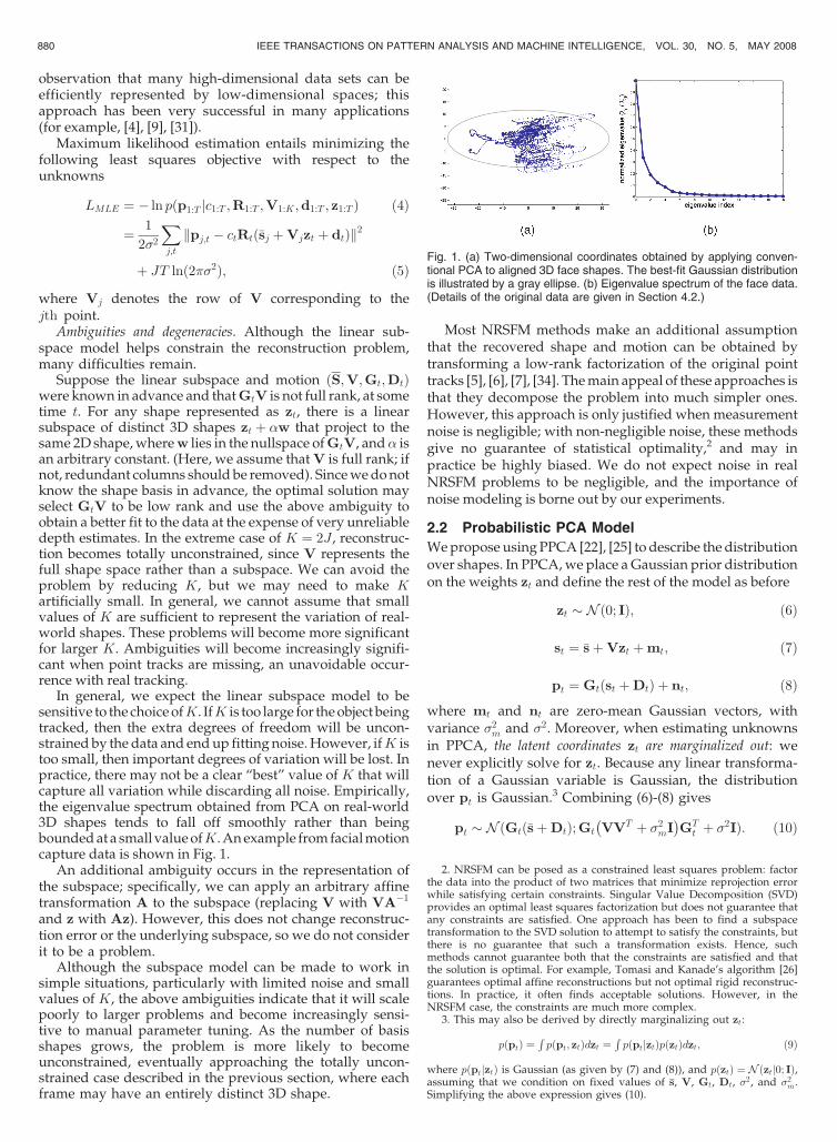
In general, we expect the linear subspace model to besensitive to the choice ofK. IfK is too large for the object beingtracked, then the extra degrees of freedom will be uncon-strained by the data and end up fitting noise. However, ifK istoo small, then important degrees of variation will be lost. Inpractice, there may not be a clear “best” value of K that willcapture all variation while discarding all noise. Empirically,the eigenvalue spectrum obtained from PCA on real-world3D shapes tends to fall off smoothly rather than beingbounded at a small value ofK. An example from facial motioncapture data is shown in Fig. 1.

An additional ambiguity occurs in the representation ofthe subspace; specifically, we can apply an arbitrary affinetransformation A to the subspace (replacing V with VA�1

and z with Az). However, this does not change reconstruc-tion error or the underlying subspace, so we do not considerit to be a problem.

Although the subspace model can be made to work insimple situations, particularly with limited noise and smallvalues of K, the above ambiguities indicate that it will scalepoorly to larger problems and become increasingly sensi-tive to manual parameter tuning. As the number of basisshapes grows, the problem is more likely to becomeunconstrained, eventually approaching the totally uncon-strained case described in the previous section, where eachframe may have an entirely distinct 3D shape.

Most NRSFM methods make an additional assumptionthat the recovered shape and motion can be obtained bytransforming a low-rank factorization of the original pointtracks [5], [6], [7], [34]. The main appeal of these approaches isthat they decompose the problem into much simpler ones.However, this approach is only justified when measurementnoise is negligible; with non-negligible noise, these methodsgive no guarantee of statistical optimality,2 and may inpractice be highly biased. We do not expect noise in realNRSFM problems to be negligible, and the importance ofnoise modeling is borne out by our experiments.

2.2 Probabilistic PCA Model

We propose using PPCA [22], [25] to describe the distributionover shapes. In PPCA, we place a Gaussian prior distributionon the weights zt and define the rest of the model as before

zt � Nð0; IÞ; ð6Þ

st ¼ �sþVzt þmt; ð7Þ

pt ¼ Gtðst þDtÞ þ nt; ð8Þ

where mt and nt are zero-mean Gaussian vectors, withvariance �2

m and �2. Moreover, when estimating unknownsin PPCA, the latent coordinates zt are marginalized out: wenever explicitly solve for zt. Because any linear transforma-tion of a Gaussian variable is Gaussian, the distributionover pt is Gaussian.3 Combining (6)-(8) gives

pt � NðGtð�sþDtÞ; Gt VVT þ �2mI

� �GTt þ �2IÞ: ð10Þ


2. NRSFM can be posed as a constrained least squares problem: factorthe data into the product of two matrices that minimize reprojection errorwhile satisfying certain constraints. Singular Value Decomposition (SVD)provides an optimal least squares factorization but does not guarantee thatany constraints are satisfied. One approach has been to find a subspacetransformation to the SVD solution to attempt to satisfy the constraints, butthere is no guarantee that such a transformation exists. Hence, suchmethods cannot guarantee both that the constraints are satisfied and thatthe solution is optimal. For example, Tomasi and Kanade’s algorithm [26]guarantees optimal affine reconstructions but not optimal rigid reconstruc-tions. In practice, it often finds acceptable solutions. However, in theNRSFM case, the constraints are much more complex.

3. This may also be derived by directly marginalizing out zt:

pðptÞ ¼Rpðpt; ztÞdzt ¼

RpðptjztÞpðztÞdzt; ð9Þ

where pðptjztÞ is Gaussian (as given by (7) and (8)), and pðztÞ ¼ N ðztj0; IÞ,assuming that we condition on fixed values of s, V, Gt, Dt, �

2, and �2m.

Simplifying the above expression gives (10).

Fig. 1. (a) Two-dimensional coordinates obtained by applying conven-tional PCA to aligned 3D face shapes. The best-fit Gaussian distributionis illustrated by a gray ellipse. (b) Eigenvalue spectrum of the face data.(Details of the original data are given in Section 4.2.)

In this model, solving NRSFM—estimating motion whilelearning the deformation basis—is a special form ofestimating a Gaussian distribution. In particular, we simplymaximize the joint likelihood of the measurements p1:T or,equivalently, the negative logarithm of the joint likelihood

L ¼ 1

2

Xt

ðpt � ðGtð�sþDtÞÞT ðGtðVVT þ �2mIÞGT

t þ �2IÞ

ðpt � ðGtð�sþDtÞÞ

þ 1

2

Xt

ln��GtðVVT þ �2

mIÞGTt þ �2I

��þ JT lnð2�Þ:

ð11Þ

We will describe an estimation algorithm in Section 3.2.Intuitively, the NRSFM problem can be stated as solving

for shape and motion such that the reconstructed 3D shapesare as “similar” to each other as possible. In this model,shapes arise from a Gaussian distribution with mean s andcovariance VVT þ �2

mI. Maximizing the likelihood of thedata simultaneously optimizes the 3D shapes according toboth the measurements and the Gaussian prior over shapeswhile adjusting the Gaussian prior to fit the individualshapes. An alternative approach would be to explicitly learn a3J � 3J covariance matrix. However, this involves manymore parameters than necessary, whereas PPCA provides areduced-dimensionality representation of a Gaussian. Thismodel provides several advantages over the linear subspacemodel. First, the Gaussian prior on zt represents an explicitassumption that the latent coordinates zt for each pose will besimilar to each other, that is, the zt coordinates are notunconstrained. Empirically, we find this assumption to bejustified. For example, Fig. 1 shows 2D coordinates for3D shapes taken from a facial motion capture sequence,computed by conventional PCA. These coordinates do notvary arbitrarily but remain confined to a small region ofspace. In general, we find this observation consistent whenapplying PCA to many different types of data sets. ThisGaussian prior resolves the important ambiguities describedin the previous section. Depth and scaling ambiguities areresolved by preferring shapes with smaller magnitudes of zt.The model is robust to large or misspecified values ofK, sincevery small variances will be learned for extraneous dimen-sions. A rotational ambiguity remains: replacing V and z withVAT and Az (for any orthonormal matrix A) does not changethe likelihood. However, this ambiguity has no impact on theresulting distribution over 3D shapes and can be ignored.

Second, this model accounts for uncertainty in the latentcoordinates zt. These coordinates are often underconstrainedin some axes and cannot necessarily be reliably estimated,especially during the early stages of optimization. Moreover,a concern with largeK is the large number of unknowns in theproblem, including K elements of zt for each time t.Marginalizing over these coordinates removes these vari-ables from estimation. Removing these unknowns also makesit possible to learn all model parameters—including the priorand noise terms—simultaneously without overfitting. Thismeans that regularization terms need not be set manually foreach problem and can thus be much more sophisticated andhave many more parameters than otherwise. In practice, wefind that this leads to significantly improved reconstructionsover user-specified shape PDFs. It might seem that, since theparameters of the PDF are not known a priori, the algorithm

could estimate wildly varying shapes and then learn acorrespondingly spread-out PDF. However, such a spread-out PDF would assign very low likelihood to the solution andthus be suboptimal; this is a typical case of Bayesian inferenceautomatically employing “Occam’s Razor” [19]: data fitting isautomatically balanced against the model simplicity. Oneway to see this is to consider the terms of the log probability in(11): the first term is a data-fitting term, and the second term isa regularization term that penalizes spread-out Gaussians.Hence, the optimal solution trades-off between 1) fitting thedata, 2) regularizing by penalizing distance between shapesand the shape PDF, and 3) minimizing the variance of theshape PDF as much as possible. The algorithm simulta-neously regularizes and learns the regularization.

Regularized linear subspace model. An alternative approachto resolving ambiguities is to introduce regularization termsthat penalize large deformations. For example, if we solvefor latent coordinates zt in the above model rather thanmarginalizing them out, then the corresponding objectivefunction becomes

LMAP ¼ � ln pðp1:T jR1:T ;V1:K;d1:T ; z1:T Þ

¼ 1

2�2

Xj;t

kpj;t � ctRtð�sj þVjzt þ dtÞk2 ð12Þ

þ 1

2�2z

Xt

kztk2 þ JT2

lnð2��2Þ þ TK2

lnð2��2zÞ; ð13Þ

which is the same objective function, as in (5) with theaddition of a quadratic regularizer on zt. However, thisobjective function is degenerate. To see this, consider anestimate of the basis V and latent coordinates z1:T . If wescale all of these terms as

V 2V; zt 1

2zt; ð14Þ

then the objective function must decrease. Consequently,this objective function is optimized by infinitesimal latentcoordinates but without any improvement to the recon-structed 3D shapes.

Previous work in this area has used various combinationsof regularization terms [5], [29]. Designing appropriateregularization terms and choosing their weights is generallynot easy; we could place a prior on the basis (for example,penalize the Frobenius norm of V), but it is not clear how tobalance the weights of the different regularization terms; forexample, the scale of the V weight will surely depend on thescale of the specific problem being addressed. One couldrequire the basis to be orthonormal, but this leads to anisotropic Gaussian distribution, unless separate varianceswere specified for every latent dimension. One could alsoattempt to learn the weights together with the model, but thiswould almost certainly be underconstrained with so manymore unknown parameters than measurements. In contrast,our PPCA-based approach avoids these difficulties withoutrequiring any additional assumptions or regularization.

2.3 Linear Dynamics Model

In many cases, point tracking data comes from sequentialframes of a video sequence. In this case, there is an additionaltemporal structure in the data that can be modeled in thedistribution over shapes. For example, 3D human facialmotion shown in 2D PCA coordinates in Fig. 1 shows distinct


temporal structure: the coordinates move smoothly through

the space, rather than appearing as random independent and

identically distributed (IID) samples from a Gaussian.Here, we model temporal structure with a linear dynami-

cal model of shape

z1 � Nð0; IÞ; ð15Þzt ¼ �zt�1 þ vt; vt � Nð0; QÞ: ð16Þ

In this model, the latent coordinates zt at each time step are

produced by a linear function of the previous time step,

based on the K �K transition matrix �, plus additive

Gaussian noise with covariance Q. Shapes and observations

are generated as before

st ¼ �sþVzt þmt; ð17Þpt ¼ Gtðst þDtÞ þ nt: ð18Þ

As before, we solve for all unknowns except for the latent

coordinates z1:T , which are marginalized out. The algorithm

is described in Section 3.3. This algorithm learns 3D shape

with temporal smoothing while simultaneously learning the

smoothness terms.

3 ALGORITHMS

3.1 Least Squares NRSFM with a Linear SubspaceModel

As a baseline algorithm, we introduce a technique that

optimizes the least squares objective function (5) with block

coordinate descent. This method, which we refer to as BCD-

LS, was originally presented in [29]. No prior assumption is

made about the distribution of the latent coordinates, and

so, the weak-perspective scaling factor ct can be folded into

the latent coordinates by representing the shape basis as

~V � ½�s;V�; ~zct � ct½1; zTt �T : ð19Þ

We then optimize directly for these unknowns. Addition-

ally, since the depth component of rigid translation is

unconstrained, we estimate 2D translations Tt � GtDt ¼½ctRtdt; . . . ; ctRtdt� � ½tt; . . . ; tt�. The variance terms are

irrelevant in this formulation and can be dropped from (5),

yielding the following two equivalent forms:

LMLE ¼Xj;t

kpj;t �Rt~Vj~z

ct � ttk2 ð20Þ

¼Xt

kpt �Ht~V~zct �Ttk2; ð21Þ

where Ht is a 2J � 3J matrix containing J copies of Rt

across the diagonal.This objective is optimized by coordinate descent

iterations applied to subsets of the unknowns. Each of

these steps finds the global optimum of the objective

function with respect to a specific block of the parameters

while holding the others fixed. Except for the rotation

parameters, each update can be solved in closed form.

For example, the update to tt is derived by solving

@LMLE=@tt ¼ �2P

jðpj;t �Rt~Vj~z

ct � ttÞ ¼ 0. The updates

are as follows:

vecð ~VjÞ Mþðpj;1:T �TtÞ; ð22Þ~zct ðHt

~VÞþðpt �TtÞ; ð23Þ

tt 1

J

Xj

ðpj;t �Rt~Vj~z

ctÞ; ð24Þ

where pj;1:T ¼ ½pTj;1; . . . ;pTj;T �T , M ¼ ½~zc1 �RT

1 ; . . . ; ~zcT �RTT �T ,

� denotes Kronecker product, and the vec operator stacksthe entries of a matrix into a vector.4 The shape basis updateis derived by rewriting the objective as

LMLE /Xj

kpj;1:T �Mvecð ~VjÞ �Ttk2 ð25Þ

and by solving @LMLE=@vecð ~VjÞ ¼ 0.The camera matrix Rt is subject to a nonlinear orthonorm-

ality constraint and cannot be updated in closed form.Instead, we perform a single Gauss-Newton step. First, weparameterize the current estimate of the motion with a3� 3 rotation matrix Qt, so that Rt ¼ �Qt, where

� ¼ 1 0 00 1 0

� �:

We define the updated rotation relative to the previousestimate as Qnew

t ¼ �QtQt. The incremental rotation �Qt

is parameterized in exponential map coordinates by a3D vector �t ¼ ½!xt ; !

yt ; !

zt �T

�Qt¼ e�t ¼ Iþ �t þ �2

t =2!þ . . . ; ð26Þ

where �t denotes the skew-symmetric matrix

�t ¼0 �!zt !yt!zt 0 �!xt�!yt !xt 0

24

35: ð27Þ

Dropping nonlinear terms gives the updated value asQnewt ¼ ðIþ �tÞQt. Substituting Qnew

t into (20) gives

LMLE /Xj;t

kpj;t ��ðIþ �tÞQt~Vj~z

ct � ttk2 ð28Þ

/Xj;t

k��taj;t � bj;tk2; ð29Þ

where aj;t ¼ Qt~Vj~z

ct and bj;t ¼ ðpj;t �Rt

~Vj~zct � ttÞ. Let

aj;t ¼½axj;t; ayj;t; a

zj;t�

T . Note that we can write the matrix

product ��taj;t directly in terms of the unknown twist vector

�t ¼ ½!xt ; !yt ; !

zt �T :

��taj;t ¼0 �!zt !yt

!zt 0 �!xt

� � axj;t

ayj;tazj;t

264

375 ð30Þ

¼0 azj;t ayj;t�azj;t 0 axj;t

" #�t: ð31Þ

We use this identity to solve for the twist vector �tminimizing (29):

�t ¼Xj

CTj;tCj;t

!�1 Xj

CTj;tbj;t

!; ð32Þ


4. For example, veca0 a2

a1 a3

� �� ¼ ½a0; a1; a2; a3�T .

where

Cj;t ¼ 0 azj;t ayj;t�azj;t 0 axj;t

� �: ð33Þ

We finally compute the updated rotation as Qnewt e�tQt,

which is guaranteed to satisfy the orthonormality constraint.Note that, since each of the parameter updates involves the

solution of an overconstrained linear system, BCD-LS can beused even when some of the point tracks are missing. In suchevent, the optimization is carried out over the available data.

The rigid motion is initialized by the Tomasi-Kanade [26]algorithm; the latent coordinates are initialized randomly.

3.2 NRSFM with PPCA

We now describe an EM algorithm to estimate the PPCAmodel from point tracks. The EM algorithm is a standardoptimization algorithm for latent variable problems [12];our derivation follows closely those for PPCA [22], [25] andfactor analysis [14]. Given tracking data p1:T , we seek toestimate the unknowns G1:T , T1:T , s, V, and �2 (as before,we estimate 2D translations T, due to the depth ambiguity).To simplify the model, we remove one source of noise byassuming �2

m ¼ 0. The data likelihood is given by

pðp1:T jG1:T ;T1:T ;�s;V; �2Þ ¼

Yt

pðptjGt;Tt;�s;V; �2Þ; ð34Þ

where the per-frame distribution is Gaussian (8). Addition-ally, if there are any missing point tracks, these will also beestimated. The EM algorithm alternates between two steps:in the E step, a distribution over the latent coordinates zt iscomputed; in the M step, the other variables are updated.5

E-step. In the E step, we compute the posterior distribu-tion over the latent coordinates zt given the currentparameter estimates, for each time t. Defining qðztÞ to bethis distribution, we have

qðztÞ ¼ pðztjpt;Gt;Tt;�s;V; �2Þ ð35Þ

¼ N ðztj�ðpt �Gt�s�TtÞÞ; I� �GtVÞ; ð36Þ� ¼ VTGT

t ðGtVVTGTt þ �2IÞ�1: ð37Þ

The computation of � may be accelerated by the MatrixInversion lemma

� ¼ ��2I�GtVðIþ ��2VTGTt GtVÞ�1VTGT

t ��4: ð38Þ

Given this distribution, we also define the followingexpectations:

�t � E½zt� ¼ �ðpt �Gt�s�TtÞ; ð39Þ�t � E½ztzTt � ¼ I� �GtVþ �t�Tt ; ð40Þ

where the expectation is taken with respect to qðztÞ.M-step. In the M step, we update the motion parameters

by minimizing the expected negative log likelihood:

Q � E½� log pðp1:T jG1:T ;T1:T ;�s;V; �2Þ� ð41Þ

¼ 1

2�2

Xt

E½kpt�ðGtð�sþVztÞ�TtÞk2� þ JT logð2��2Þ:ð42Þ

This function cannot be minimized in closed form, but closedform updates can be computed for each of the individualparameters (except for the camera parameters, discussedbelow). To make the updates more compact, we define thefollowing additional variables:

~V � ½�s;V�; ~zt � ½1; zTt �T ; ð43Þ

~�t � ½1; �Tt �T ; ~�t �

1 �Tt�t �t

� �: ð44Þ

The unknowns are then updated as follows; derivations aregiven in the Appendix.

vecð ~VÞ Xt

ð ~�Tt � ðGTt GtÞÞ

!�1

vecXt

GTt ðpt �TtÞ~�Tt

!;

ð45Þ

�2 1

2JT

Xt

kpt �Ttk2 � 2ðpt �TtÞTGt~V~�tþ

ð46Þ

tr ~VTGTt Gt

~V ~�t� ��

; ð47Þ

ct Xj

~�Tt~VTj RT

t ðpj;t�ttÞ=Xj

tr ~VTj RT

t RTt

~Vj~�t

; ð48Þ

tt 1

J

Xj

pj;t � ctRt~Vj~�t

� �: ð49Þ

The system of equations for the shape basis update islarge and sparse, so we compute the shape update usingconjugate gradient.

The camera matrix Rt is subject to a nonlinear orthonorm-ality constraint and cannot be updated in closed form.Instead, we perform a single Gauss-Newton step. First, weparameterize the current estimate of the motion with a3� 3 rotation matrix Qt, so that Rt ¼ �Qt, where

� ¼ 1 0 00 1 0

� �:

The update is then

vecð�Þ AþB; ð50ÞRt �e�Qt; ð51Þ

where A and B are given in (70) and (71).If the input data is incomplete, the missing tracks are

filled in during the M step of the algorithm. Let point pj0;t0be one of the missing entries in the 2D tracks. Optimizingthe expected log likelihood with respect to the unobservedpoint yields the update rule

pj0;t0 ct0Rt0~Vj0 ~�t0 þ tt0: ð52Þ

Once the model is learned, the maximum likelihood 3D shapefor frame t is given by sþV�t; in camera coordinates, it isctQtðsþV�t þDtÞ. (The depth component of Dt cannot bedetermined and, thus, is set to zero).

Initialization. The rigid motion is initialized by the Tomasi-Kanade [26] algorithm. The first component of the shapebasis V is initialized by fitting the residual using separate


5. Technically, our algorithm is an instance of the Generalized EMalgorithm, since our M step does not compute a global optimum of theexpected log likelihood.

shapes St at each time step (holding the rigid motion fixed)and then applying PCA to these shapes. This process isiterated (that is, the second component is fit based on theremaining residual, and so forth) to produce an initialestimate of the entire basis. We found the algorithm to belikely to converge to a good minimum when �2 is forced toremain large in the initial steps of the optimization. For thispurpose, we scale �2 with an annealing parameter thatdecreases linearly with the iteration count and finishes at 1.

3.3 NRSFM with Linear Dynamics

The linear dynamical model introduced in Section 2.3 forNRSFM is a special form of a general LDS. Shumway andStoffer [15], [23] describe an EM algorithm for this case,which can be directly adapted to our problem. Thesufficient statistics �t, �t, and E½ztzTt�1� can be computedwith Shumway and Stoffer’s E step algorithm, whichperforms a linear-time Forward-Backward algorithm; theforward step is equivalent to Kalman filtering. In theM step, we perform the same shape update steps as above;moreover, we update the � and Q matrices using Shumwayand Stoffer’s update equations.

4 EXPERIMENTS

We now describe quantitative experiments comparingNRSFM algorithms on both synthetic and real data sets.Here, we compare the following models and algorithms:6

. BCD-LS. The least squares algorithm described inSection 3.1.

. EM-PPCA. The PPCA model using the EM algo-rithm described in Section 3.2.

. EM-LDS. The LDS model using the EM algorithmdescribed in Section 3.3.

. XCK. The closed-form method by Xiao et al. [34].

. B05. Brand’s “direct” method [6].

We do not consider here the original algorithm by Bregleret al. [7], since we and others have found it to giveinferior results to all subsequent methods; we also omitBrand’s factorization method [5] from consideration.

To evaluate results, we compare the sum of squareddifferences between estimated 3D shapes to ground-truthdepth: ksC1:T � sC1:TkF , measured in the camera coordinatesystem (that is, applying the camera rotation, translation, andscale). In order to avoid an absolute depth ambiguity, wesubtract out the centroid of each shape before comparing. Inorder to account for a reflection ambiguity, we repeat the testwith the sign of depth inverted (�Z instead of Z) for eachinstant and take the smaller error. In the experimentsinvolving noise added to the input data, we perturbed the2D tracks with additive Gaussian noise. The noise level isplotted as the ratio of the noise variance to the norm of the2D tracks, that is, JT�2=kp1:TkF . Errors are averaged over20 runs.

4.1 Synthetic Data

We performed experiments using two synthetic data sets. Thefirst is a data set created by Xiao et al. [34], containing six rigidpoints (arranged in the shape of a cube) and three linearlydeforming points, without noise. As reported previously, the

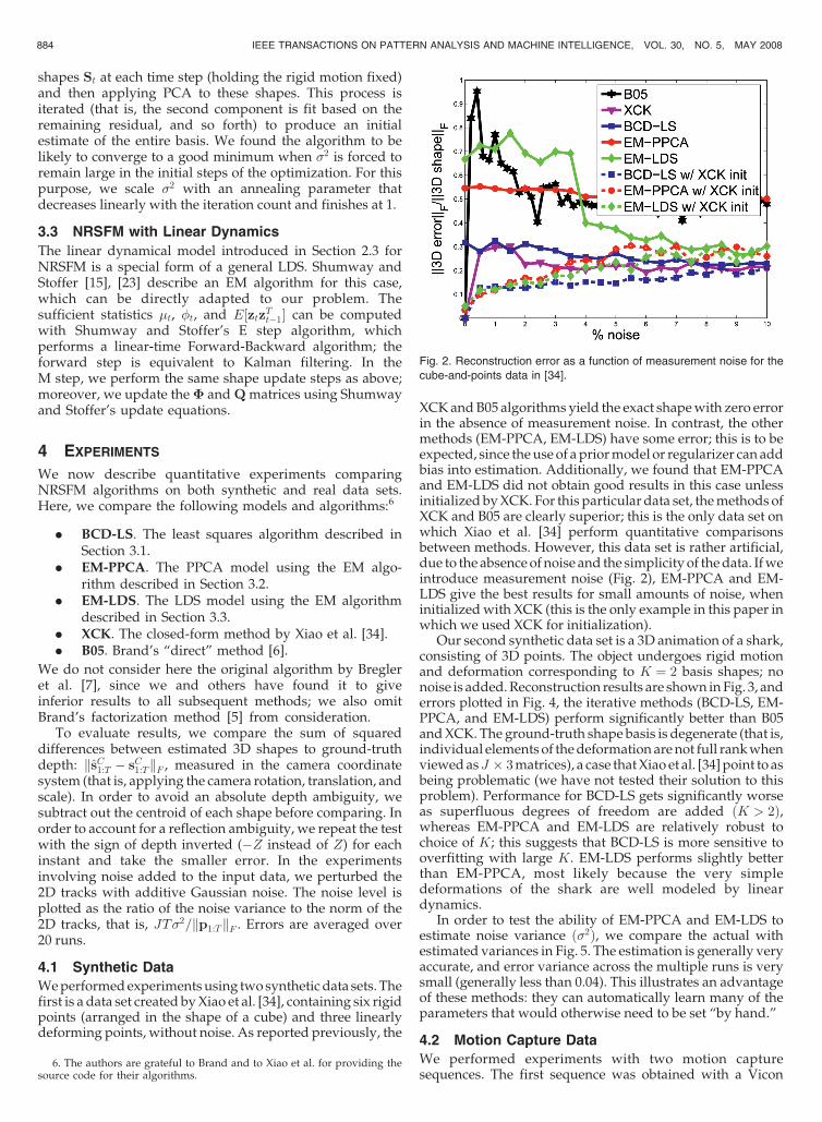
XCK and B05 algorithms yield the exact shape with zero errorin the absence of measurement noise. In contrast, the othermethods (EM-PPCA, EM-LDS) have some error; this is to beexpected, since the use of a prior model or regularizer can addbias into estimation. Additionally, we found that EM-PPCAand EM-LDS did not obtain good results in this case unlessinitialized by XCK. For this particular data set, the methods ofXCK and B05 are clearly superior; this is the only data set onwhich Xiao et al. [34] perform quantitative comparisonsbetween methods. However, this data set is rather artificial,due to the absence of noise and the simplicity of the data. If weintroduce measurement noise (Fig. 2), EM-PPCA and EM-LDS give the best results for small amounts of noise, wheninitialized with XCK (this is the only example in this paper inwhich we used XCK for initialization).

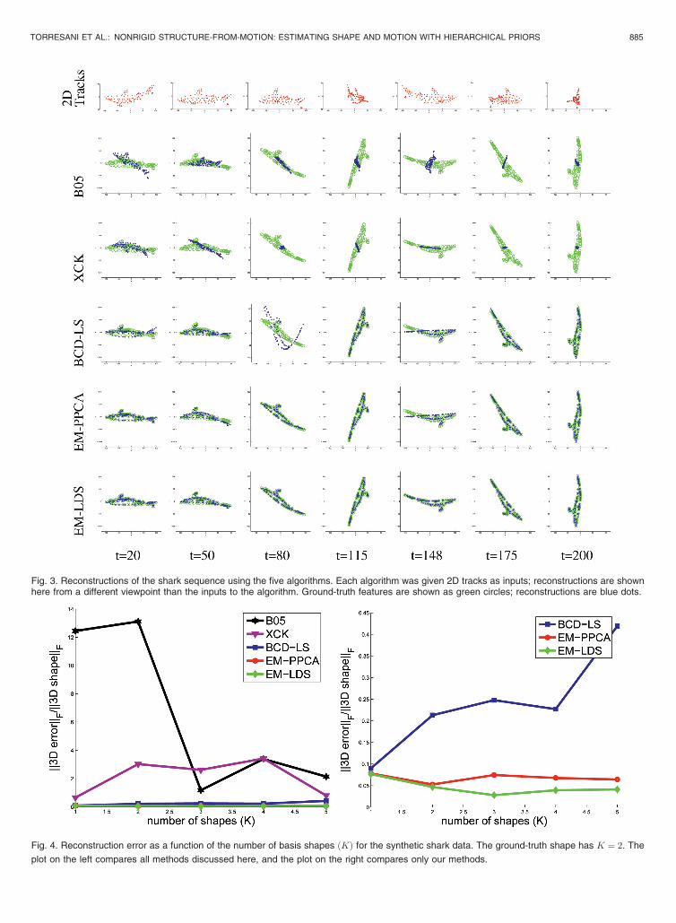
Our second synthetic data set is a 3D animation of a shark,consisting of 3D points. The object undergoes rigid motionand deformation corresponding to K ¼ 2 basis shapes; nonoise is added. Reconstruction results are shown in Fig. 3, anderrors plotted in Fig. 4, the iterative methods (BCD-LS, EM-PPCA, and EM-LDS) perform significantly better than B05and XCK. The ground-truth shape basis is degenerate (that is,individual elements of the deformation are not full rank whenviewed asJ � 3 matrices), a case that Xiao et al. [34] point to asbeing problematic (we have not tested their solution to thisproblem). Performance for BCD-LS gets significantly worseas superfluous degrees of freedom are added ðK > 2Þ,whereas EM-PPCA and EM-LDS are relatively robust tochoice of K; this suggests that BCD-LS is more sensitive tooverfitting with large K. EM-LDS performs slightly betterthan EM-PPCA, most likely because the very simpledeformations of the shark are well modeled by lineardynamics.

In order to test the ability of EM-PPCA and EM-LDS toestimate noise variance ð�2Þ, we compare the actual withestimated variances in Fig. 5. The estimation is generally veryaccurate, and error variance across the multiple runs is verysmall (generally less than 0.04). This illustrates an advantageof these methods: they can automatically learn many of theparameters that would otherwise need to be set “by hand.”

4.2 Motion Capture Data

We performed experiments with two motion capturesequences. The first sequence was obtained with a Vicon


6. The authors are grateful to Brand and to Xiao et al. for providing thesource code for their algorithms.

Fig. 2. Reconstruction error as a function of measurement noise for the

cube-and-points data in [34].


Fig. 3. Reconstructions of the shark sequence using the five algorithms. Each algorithm was given 2D tracks as inputs; reconstructions are shownhere from a different viewpoint than the inputs to the algorithm. Ground-truth features are shown as green circles; reconstructions are blue dots.

Fig. 4. Reconstruction error as a function of the number of basis shapes ðKÞ for the synthetic shark data. The ground-truth shape has K ¼ 2. The

plot on the left compares all methods discussed here, and the plot on the right compares only our methods.

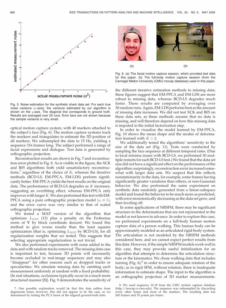
optical motion capture system, with 40 markers attached tothe subject’s face (Fig. 6). The motion capture systems trackthe markers and triangulates to estimate the 3D position ofall markers. We subsampled the data to 15 Hz, yielding asequence 316 frames long. The subject performed a range offacial expressions and dialogue. Test data is generated byorthographic projection.

Reconstruction results are shown in Fig. 7 and reconstruc-tion error plotted in Fig. 8. As is visible in the figure, the XCKand B05 algorithms both yield unsatisfactory reconstruc-tions,7 regardless of the choice of K, whereas the iterativemethods (BCD-LS, EM-PPCA, EM-LDS) perform signifi-cantly better. EM-PPCA yields the best results on the originaldata. The performance of BCD-LS degrades as K increases,suggesting an overfitting effect, whereas EM-PPCA onlyimproves with largerK. We also performed this test with EM-PPCA using a pure orthographic projection model ðct � 1Þ,and the error curve was very similar to that of scaledorthographic projection.

We tested a MAP version of the algorithm thatoptimizes LMAP (13) plus a penalty on the Frobeniusnorm of V by block coordinate descent. We found thismethod to give worse results than the least squaresoptimization (that is, optimizing LMLE by BCD-LS), for allregularization weights that we tested. This suggests thatselecting appropriate regularization is not trivial.

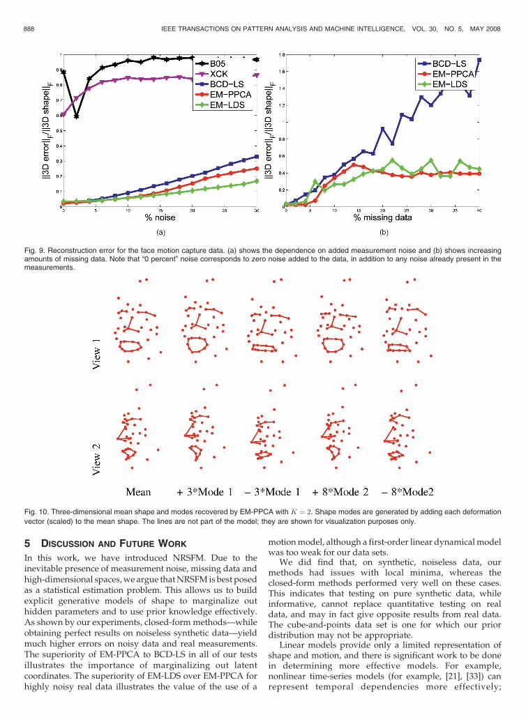
We also performed experiments with noise added to thedata and with random tracks removed. The missing data caseis important to test, because 3D points will necessarilybecome occluded in real-image sequences and may also“disappear” for other reasons such as dropped tracks orspecularities. We simulate missing data by omitting eachmeasurement uniformly at random with a fixed probability.(In real situations, occlusions typically occur in a much morestructured manner [8]). Fig. 9 demonstrates the sensitivity of

the different iterative estimation methods to missing data;these figures suggest that EM-PPCA and EM-LDS are morerobust to missing data, whereas BCD-LS degrades muchfaster. These results are computed by averaging over30 random runs. Again, EM-LDS performs best as the amountof missing data increases. We did not test XCK and B05 onthese data sets, as these methods assume that no data ismissing, and will therefore depend on how this missing datais imputed in the initial factorization step.

In order to visualize the model learned by EM-PPCA,Fig. 10 shows the mean shape and the modes of deforma-tion learned with K ¼ 2.

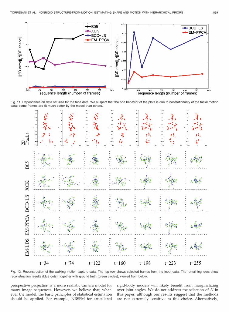
We additionally tested the algorithms’ sensitivity to thesize of the data set (Fig. 11). Tests were conducted bysampling the face sequence at different temporal rates. (Dueto local minima issues with BCD-LS, we performed 30 mul-tiple restarts for each BCD-LS test.) We found that the data setsize did not have a significant effect on the performance of thealgorithm; surprisingly, reconstruction error increased some-what with larger data sets. We suspect that this reflectsnonstationarity in the data, for example, some frames havingsignificantly greater variations than others, or non-Gaussianbehavior. We also performed the same experiment onsynthetic data randomly generated from a linear-subspacemodel and found the behavior to be much more as predicted,with error monotonically decreasing as the data set grew, andthen leveling off.

In some applications of NRSFM, there may be significantstructure in the deformations that are not represented in themodel or not known in advance. In order to explore this case,we performed experiments on a full-body human motioncapture data of a person walking. This human body can beapproximately modeled as an articulated rigid-body system.The articulation is not modeled by the NRSFM methodsconsidered here, and we cannot expect perfect results fromthis data. However, if the simple NRSFM models work well inthis case, they may provide useful initialization for analgorithm that attempts to determine the articulation struc-ture or the kinematics. We chose walking data that includesturning (Fig. 6),8 in order to ensure adequate rotation of thebody; as in rigid SFM, without rotation, there is inadequateinformation to estimate shape. The input to the algorithm isan orthographic projection of 3D marker measurements.


Fig. 6. (a) The facial motion capture session, which provided test datafor this paper. (b) The full-body motion capture session (from theCarnegie Mellon University (CMU) mocap database) used in this paper.

7. One possible explanation would be that this data suffers fromdegenerate bases; however, this did not appear to be the case, as wedetermined by testing the PCA bases of the aligned ground-truth data.

8. We used sequence 16-18 from the CMU motion capture database(http://mocap.cs.cmu.edu). The sequence was subsampled by discardingevery other frame and most of the markers. The resulting data has260 frames and 55 points per frame.

Fig. 5. Noise estimation for the synthetic shark data set. For each truenoise variance (x-axis), the variance estimated by our algorithm isshown on the y-axis. The diagonal line corresponds to ground truth.Results are averaged over 20 runs. Error bars are not shown becausethe sample variance is very small.

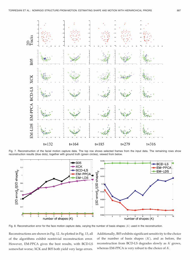
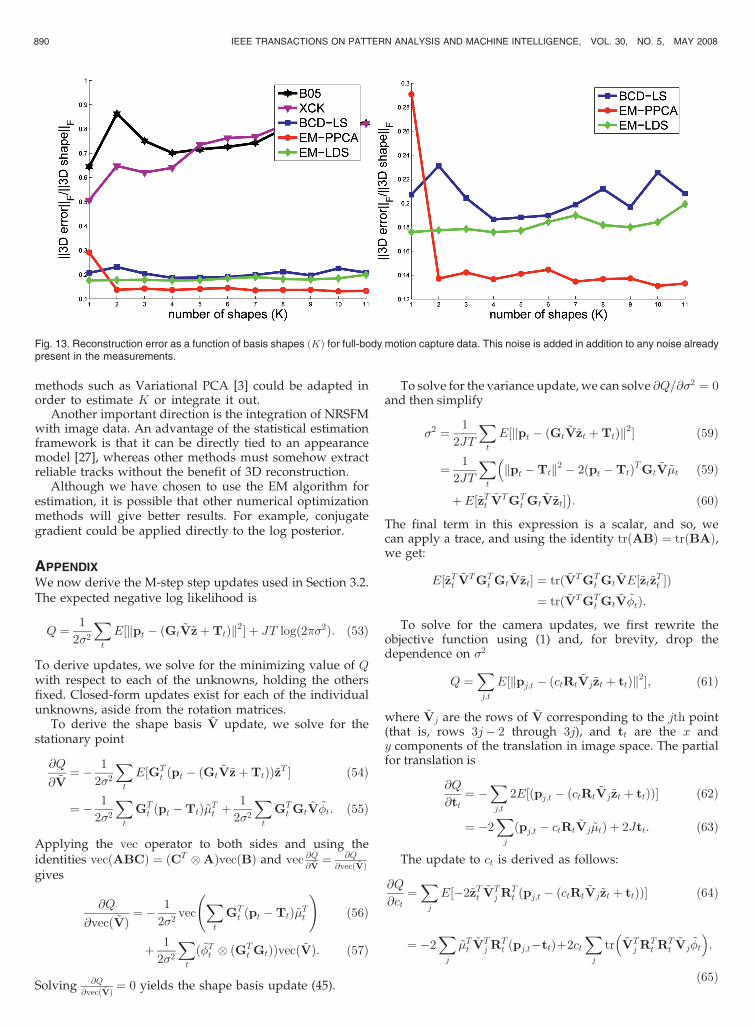
Reconstructions are shown in Fig. 12. As plotted in Fig. 13, all

of the algorithms exhibit nontrivial reconstruction error.

However, EM-PPCA gives the best results, with BCD-LS

somewhat worse; XCK and B05 both yield very large errors.

Additionally, B05 exhibits significant sensitivity to the choice

of the number of basis shapes ðKÞ, and as before, the

reconstruction from BCD-LS degrades slowly as K grows,

whereas EM-PPCA is very robust to the choice of K.


Fig. 7. Reconstruction of the facial motion capture data. The top row shows selected frames from the input data. The remaining rows showreconstruction results (blue dots), together with ground truth (green circles), viewed from below.

Fig. 8. Reconstruction error for the face motion capture data, varying the number of basis shapes ðKÞ used in the reconstruction.

5 DISCUSSION AND FUTURE WORK

In this work, we have introduced NRSFM. Due to theinevitable presence of measurement noise, missing data andhigh-dimensional spaces, we argue that NRSFM is best posedas a statistical estimation problem. This allows us to buildexplicit generative models of shape to marginalize outhidden parameters and to use prior knowledge effectively.As shown by our experiments, closed-form methods—whileobtaining perfect results on noiseless synthetic data—yieldmuch higher errors on noisy data and real measurements.The superiority of EM-PPCA to BCD-LS in all of our testsillustrates the importance of marginalizing out latentcoordinates. The superiority of EM-LDS over EM-PPCA forhighly noisy real data illustrates the value of the use of a

motion model, although a first-order linear dynamical modelwas too weak for our data sets.

We did find that, on synthetic, noiseless data, ourmethods had issues with local minima, whereas theclosed-form methods performed very well on these cases.This indicates that testing on pure synthetic data, whileinformative, cannot replace quantitative testing on realdata, and may in fact give opposite results from real data.The cube-and-points data set is one for which our priordistribution may not be appropriate.

Linear models provide only a limited representation ofshape and motion, and there is significant work to be donein determining more effective models. For example,nonlinear time-series models (for example, [21], [33]) canrepresent temporal dependencies more effectively;


Fig. 9. Reconstruction error for the face motion capture data. (a) shows the dependence on added measurement noise and (b) shows increasingamounts of missing data. Note that “0 percent” noise corresponds to zero noise added to the data, in addition to any noise already present in themeasurements.

Fig. 10. Three-dimensional mean shape and modes recovered by EM-PPCA with K ¼ 2. Shape modes are generated by adding each deformation

vector (scaled) to the mean shape. The lines are not part of the model; they are shown for visualization purposes only.

perspective projection is a more realistic camera model formany image sequences. However, we believe that, what-ever the model, the basic principles of statistical estimationshould be applied. For example, NRSFM for articulated

rigid-body models will likely benefit from marginalizingover joint angles. We do not address the selection of K inthis paper, although our results suggest that the methodsare not extremely sensitive to this choice. Alternatively,


Fig. 11. Dependence on data set size for the face data. We suspect that the odd behavior of the plots is due to nonstationarity of the facial motiondata; some frames are fit much better by the model than others.

Fig. 12. Reconstruction of the walking motion capture data. The top row shows selected frames from the input data. The remaining rows show

reconstruction results (blue dots), together with ground truth (green circles), viewed from below.

methods such as Variational PCA [3] could be adapted inorder to estimate K or integrate it out.

Another important direction is the integration of NRSFMwith image data. An advantage of the statistical estimationframework is that it can be directly tied to an appearancemodel [27], whereas other methods must somehow extractreliable tracks without the benefit of 3D reconstruction.

Although we have chosen to use the EM algorithm forestimation, it is possible that other numerical optimizationmethods will give better results. For example, conjugategradient could be applied directly to the log posterior.

APPENDIX

We now derive the M-step step updates used in Section 3.2.The expected negative log likelihood is

Q ¼ 1

2�2

Xt

E½kpt � ðGt~V~zþTtÞk2� þ JT logð2��2Þ: ð53Þ

To derive updates, we solve for the minimizing value of Qwith respect to each of the unknowns, holding the othersfixed. Closed-form updates exist for each of the individualunknowns, aside from the rotation matrices.

To derive the shape basis ~V update, we solve for thestationary point

@Q

@ ~V¼ � 1

2�2

Xt

E½GTt ðpt � ðGt

~V~zþTtÞÞ~zT � ð54Þ

¼ � 1

2�2

Xt

GTt ðpt �TtÞ~�Tt þ

1

2�2

Xt

GTt Gt

~V ~�t: ð55Þ

Applying the vec operator to both sides and using theidentities vecðABCÞ ¼ ðCT �AÞvecðBÞ and vec @Q

@ ~V¼ @Q

@vecð ~VÞgives

@Q

@vecð ~VÞ¼ � 1

2�2vec

Xt

GTt ðpt �TtÞ~�Tt

!ð56Þ

þ 1

2�2

Xt

ð ~�Tt � ðGTt GtÞÞvecð ~VÞ: ð57Þ

Solving @Q

@vecð ~VÞ ¼ 0 yields the shape basis update (45).

To solve for the variance update, we can solve @Q=@�2 ¼ 0and then simplify

�2 ¼ 1

2JT

Xt

E½kpt � ðGt~V~zt þTtÞk2� ð59Þ

¼ 1

2JT

Xt

kpt �Ttk2 � 2ðpt �TtÞTGt~V~�t

ð59Þ

þ E½~zTt ~VTGTt Gt

~V~zt��: ð60Þ

The final term in this expression is a scalar, and so, wecan apply a trace, and using the identity trðABÞ ¼ trðBAÞ,we get:

E½~zTt ~VTGTt Gt

~V~zt� ¼ trð ~VTGTt Gt

~VE½~zt~zTt �Þ¼ trð ~VTGT

t Gt~V ~�tÞ:

To solve for the camera updates, we first rewrite theobjective function using (1) and, for brevity, drop thedependence on �2

Q ¼Xj;t

E½kpj;t � ðctRt~Vj~zt þ ttÞk2�; ð61Þ

where ~Vj are the rows of ~V corresponding to the jth point(that is, rows 3j� 2 through 3j), and tt are the x andy components of the translation in image space. The partialfor translation is

@Q

@tt¼ �

Xj;t

2E½ðpj;t � ðctRt~Vj~zt þ ttÞÞ� ð62Þ

¼ �2Xj

ðpj;t � ctRt~Vj ~�tÞ þ 2Jtt: ð63Þ

The update to ct is derived as follows:

@Q

@ct¼Xj

E½�2~zTt~VTj RT

t ðpj;t � ðctRt~Vj~zt þ ttÞÞ� ð64Þ

¼ �2Xj

~�Tt~VTj RT

t ðpj;t�ttÞþ2ctXj

tr ~VTj RT

t RTt

~Vj~�t

:

ð65Þ


Fig. 13. Reconstruction error as a function of basis shapes ðKÞ for full-body motion capture data. This noise is added in addition to any noise alreadypresent in the measurements.

The camera rotation is subject to a orthonormality

constraint, for which we cannot derive a closed-form update.

Instead, we derive the following approximate update. First,

we differentiate (61)

@Q

@Rt¼ Rtc

2t

Xj

~Vj~�t ~VT

j � ctXj

ðpj;t � ttÞ~�Tt ~VTj : ð66Þ

Since we cannot obtain a closed-form solution to

@Q=@Rt ¼ 0, we linearize the rotation. We parameterize

the current rotation as a 3� 3 rotation matrix, such that

Rt ¼ �Qt, parameterize the updated rotation relative to

the previous estimate: Qnewt ¼ �QQt. The incremental

rotation �Q is parameterized by an exponential map

with twist matrix �

�Q ¼ e� ¼ Iþ � þ �2=2!þ . . . : ð67Þ

Dropping nonlinear terms gives the updated value as

Qnewt ¼ ðIþ �ÞQt. Substituting Qnew

t into (66) gives

@Q

@Rt� �ðIþ �ÞQtc

2t

Xj

~Vj~�t ~VT

j � ctXj

ðpj;t� ttÞ~�Tt ~VTj : ð68Þ

Applying the vec operator gives

vec@Q

@Rt� Avecð�Þ þB; ð69Þ

A ¼ c2t

Xj

~Vj~�t ~VT

j QTt

!��; ð70Þ

B ¼ c2t�Qt

Xj

~Vj~�t ~VT

j � ctXj

ðpj;t � ttÞ~�Tt ~VTj : ð71Þ

We minimize kAvecð�Þ þBkF with respect to � for the

update, giving vecð�Þ AþB.

ACKNOWLEDGMENTS

Earlier versions of this work appeared in [7], [28], [29].Portions of this work were conducted while L. Torresani wasat Stanford University, New York University, and Riya Inc.,while A. Hertzmann was at New York University andUniversity of Washington, and while C. Bregler was atStanford University. The authors would like to thankMatthew Brand and Jing Xiao for providing their sourcecode, Jacky Bibliowicz for providing the face mocap data, andthe Carnegie Mellon University (CMU) Motion CaptureDatabase for the full-body data. They also thank GeneAlexander, Hrishikesh Deshpande, and Danny Yang forparticipating in earlier versions of these projects. Thanks toStefano Soatto for discussing shape deformation. This workwas supported in part by the Office of Naval Research (ONR)Grant N00014-01-1-0890, US National Science Foundation(NSF) Grants IIS-0113007, 0303360, 0329098, and 0325715, theUniversity of Washington Animation Research Labs, theAlfred P. Sloan Foundation, a Microsoft Research NewFaculty Fellowship, the National Sciences and EngineeringResearch Council of Canada, the Canada Foundation forInnovation, and the Ontario Ministry of Research andInnovation. In memory of Henning Biermann.

REFERENCES

[1] J. Barbi�c and D. James, “Real-Time Subspace Integration for St.Venant-Kirchhoff Deformable Models,” ACM Trans. Graphics,vol. 24, no. 3, pp. 982-990, Aug. 2005.

[2] B. Bascle and A. Blake, “Separability of Pose and Expression inFacial Tracking Animation,” Proc. Int’l Conf. Computer Vision,pp. 323-328, Jan. 1998.

[3] C.M. Bishop, “Variational Principal Components,” Proc. Int’l Conf.Artificial Neural Networks, vol. 1, pp. 509-514, 1999.

[4] V. Blanz and T. Vetter, “A Morphable Model for the Synthesis of3D Faces,” Proc. ACM Int’l Conf. Computer Graphics and InteractiveTechniques (SIGGRAPH ’99), pp. 187-194, Aug. 1999.

[5] M. Brand, “Morphable 3D Models from Video,” Proc. ComputerVision and Pattern Recognition, vol. 2, pp. 456-463, 2001.

[6] M. Brand, “A Direct Method for 3D Factorization of NonrigidMotion Observed in 2D,” Proc. Computer Vision and PatternRecognition, vol. 2, pp. 122-128, 2005.

[7] C. Bregler, A. Hertzmann, and H. Biermann, “Recovering Non-Rigid 3D Shape from Image Streams,” Proc. Computer Vision andPattern Recognition, pp. 690-696, 2000.

[8] A.M. Buchanan and A.W. Fitzgibbon, “Damped Newton Algo-rithms for Matrix Factorization with Missing Data,” Proc.Computer Vision and Pattern Recognition, vol. 2, pp. 316-322, 2005.

[9] T.F. Cootes and C.J. Taylor, “Statistical Models of Appearance forMedical Image Analysis and Computer Vision,” Proc. SPIEMedical Imaging, 2001.

[10] J.P. Costeira and T. Kanade, “A Multibody Factorization Methodfor Independently Moving Objects,” Int’l J. Computer Vision,vol. 29, no. 3, pp. 159-179, 1998.

[11] F. Dellaert, S.M. Seitz, C.E. Thorpe, and S. Thrun, “EM, MCMC, andChain Flipping for Structure from Motion with UnknownCorrespondence,” Machine Learning, vol. 50, nos. 1-2, pp. 45-71,2003.

[12] A.P. Dempster, N.M. Laird, and D.B. Rubin, “Maximum Like-lihood from Incomplete Data via the EM Algorithm,” J. RoyalStatistical Soc. Series B, vol. 39, pp. 1-38, 1977.

[13] A. Gelman, J.B. Carlin, H.S. Stern, and D.B. Rubin, Bayesian DataAnalysis, second ed. CRC Press, 2003.

[14] Z. Ghahramani and G.E. Hinton, “The EM Algorithm for Mixturesof Factor Analyzers,” Technical Report CRG-TR-96-1, Univ. ofToronto, 1996.

[15] Z. Ghahramani and G.E. Hinton, “Parameter Estimation for LinearDynamical Systems,” Technical Report CRG-TR-96-2, Univ. ofToronto, 1996.

[16] M. Han and T. Kanade, “Multiple Motion Scene Reconstructionfrom Uncalibrated Views,” Proc. Int’l Conf. Computer Vision, vol. 1,pp. 163-170, July 2001.

[17] R. Hartley and A. Zisserman, Multiple View Geometry in ComputerVision, second ed. Cambridge Univ. Press, 2003.

[18] G. Johansson, “Visual Perception of Biological Motion and aModel for Its Analysis,” Perception and Psychophysics, vol. 14,pp. 201-211, 1973.

[19] D.J.C. MacKay, “Probable Networks and Plausible Predictions—AReview of Practical Bayesian Methods for Supervised NeuralNetworks,” Network: CNS, vol. 6, pp. 469-505, 1995.

[20] F.I. Parke, “Computer Generated Animation of Faces,” Proc. ACMAnn. Conf., pp. 451-457, 1972.

[21] V. Pavlovi�c, J.M. Rehg, and J. MacCormick, “Learning SwitchingLinear Models of Human Motion,” Advances in Neural InformationProcessing Systems 13, pp. 981-987, 2001.

[22] S.T. Roweis, “EM Algorithms for PCA and SPCA,” Proc. Ann.Conf. Advances in Neural Information Processing Systems (NIPS ’97),pp. 626-632, 1998.

[23] R.H. Shumway and D.S. Stoffer, “An Approach to Time SeriesSmoothing and Forecasting Using the EM Algorithm,” J. TimeSeries Analysis, vol. 3, no. 4, pp. 253-264, 1982.

[24] L. Sirovich and M. Kirby, “Low-Dimensional Procedure for theCharacterization of Human Faces,” J. Optical Soc. Am. A, vol. 4,no. 3, pp. 519-524, Mar. 1987.

[25] M.E. Tipping and C.M. Bishop, “Probabilistic Principal Compo-nents Analysis,” J. Royal Statistical Soc. Series B, vol. 61, no. 3,pp. 611-622, 1999.

[26] C. Tomasi and T. Kanade, “Shape and Motion from Image StreamsUnder Orthography: A Factorization Method,” Int’l J. ComputerVision, vol. 9, no. 2, pp. 137-154, 1992.


[27] L. Torresani and A. Hertzmann, “Automatic Non-Rigid 3DModeling from Video,” Proc. European Conf. Computer Vision,pp. 299-312, 2004.

[28] L. Torresani, A. Hertzmann, and C. Bregler, “Learning Non-Rigid3D Shape from 2D Motion,” Proc. Ann. Conf. Advances in NeuralInformation Processing Systems (NIPS ’04), pp. 1555-1562, 2004.

[29] L. Torresani, D. Yang, G. Alexander, and C. Bregler, “Trackingand Modeling Non-Rigid Objects with Rank Constraints,” Proc.Computer Vision and Pattern Recognition, pp. 493-500, 2001.

[30] N.F. Troje, “Decomposing Biological Motion: A Framework forAnalysis and Synthesis of Human Gait Patterns,” J. Vision, vol. 2,no. 5, pp. 371-387, 2002.

[31] M. Turk and A. Pentland, “Eigenfaces for Recognition,”J. Cognitive Neuroscience, vol. 3, no. 1, pp. 71-86, 1991.

[32] S. Ullman, “Maximizing Rigidity: The Incremental Recovery of 3-D Structure from Rigid and Nonrigid Motion,” Perception, vol. 13,no. 3, pp. 255-274, 1984.

[33] J.M. Wang, D.J. Fleet, and A. Hertzmann, “Gaussian ProcessDynamical Models,” Proc. Ann. Conf. Advances in Neural Informa-tion Processing Systems (NIPS ’06), pp. 1441-1448, 2006.

[34] J. Xiao, J. Chai, and T. Kanade, “A Closed-Form Solution to Non-Rigid Shape and Motion Recovery,” Int’l J. Computer Vision,vol. 67, no. 2, pp. 233-246, 2006.

[35] A.J. Yezzi and S. Soatto, “Deformotion: Deforming Motion, ShapeAverages, and the Joint Registration and Approximation ofStructures in Images,” Int’l J. Computer Vision, vol. 53, pp. 153-167, 2003.

Lorenzo Torresani received a degree in com-puter science from the University of Milan, Italy,in 1996 and the MS and PhD degrees incomputer science from Stanford University in2001 and 2005, respectively. He worked at RiyaInc., at the Courant Institute of New YorkUniversity, and at Digital Persona Inc. He iscurrently an associate researcher at MicrosoftResearch Cambridge and a research assistantprofessor of computer science at Dartmouth

College. His main research interests include computer vision, machinelearning, and computer animation. He was the recipient of the BestStudent Paper Prize at the IEEE Conference on Computer Vision andPattern Recognition 2001.

Aaron Hertzmann received the BA degree incomputer science and in art and art history fromRice University in 1996, and the MS and PhDdegrees in computer science from New YorkUniversity in 1998 and 2001, respectively. Heworked at the University of Washington, Micro-soft Research, Mitsubishi Electric ResearchLaboratories, Interval Research Corporation,and NEC Research Institute. He is an associateprofessor of computer science at the University

of Toronto. His research interests include computer vision, computergraphics, and machine learning. He serves as an associate editor of theIEEE Transactions on Visualization and Computer Graphics, an areacoordinator for the International Conference and Exhibition on ComputerGraphics and Interactive Techniques (SIGGRAPH) 2007, and cochairedthe International Symposium on Non-Photorealistic Animation andRendering (NPAR) 2004. His awards include an MIT TR100 in 2004,an Ontario Early Researcher Award in 2005, a Sloan FoundationFellowship in 2006, and a Microsoft New Faculty Fellowship in 2007. Heis a member of the IEEE.

Christoph Bregler received the Diplom degreefrom Karlsruhe University in 1993 and the MSand PhD degrees in computer science from theUniversity of California, Berkeley, in 1995 and1998, respectively. He is currently an associateprofessor of computer science at New YorkUniversity’s (NYU) Courant Institute. Prior toNYU, he was on the faculty of StanfordUniversity and worked for several companiesincluding Hewlett Packard, Interval, and Disney

Feature Animation. He received the Olympus Prize for achievements incomputer vision and artificial intelligence in 2002. He was named as aStanford Joyce Faculty Fellow and Terman Fellow in 1999 and SloanResearch Fellow in 2003. He was the chair of the InternationalConference on Computer Graphics and Interactive Techniques (SIG-GRAPH) 2004 Electronic Theater and Computer Animation Festival.

. For more information on this or any other computing topic,please visit our Digital Library at www.computer.org/publications/dlib.


Documents

Nonrigid Structure-from-Motion: Estimating Shape and Motion with Hierarchical Priors