Numerical and experimental analysis of masonry arches ... · Numerical and experimental analysis of masonry arches strengthened with FRP materials Maria Ricamato Cassino, Novembre

Università degli Studi di Cassino

Facoltà di Ingegneria

Dottorato di Ricerca in Ingegneria Civile

XX Ciclo

Numerical and experimental analysis of

masonry arches strengthened with FRP

materials

Maria Ricamato

Cassino, Novembre 2007

2

University of Cassino Department of Engineering

Graduate School in Civil Engineering XX Cycle - November 2007

Numerical and experimental analysis of masonry

arches strengthened with FRP materials

Maria Ricamato

Supervisor: Prof. Elio Sacco

Coordinator: Prof.ssa Maura Imbimbo

3

To my mother and my father,

with love

4

Acknowledgements

Three years ago this day seemed very distant, instead today I am working for

concluding my PhD thesis. At the end of this experience, first the financial supports

of the Italian National Research Council (CNR) and of The Laboratories University

Network of Seismic Engineering (RELUIS) are gratefully acknowledged.

My greatest thanks is for my “Scientific fathers”: Prof. Giovanni Romano for

having directed me towards the research and Prof. Elio Sacco for giving me the

opportunity to improve my scientific and technical knowledge, for the work done

under his supervision and for his useful suggestions.

I would like to thank Prof.ssa Sonia Marfia for the fruitful discussions and also

Prof.ssa Maura Imbimbo and Prof. Raimondo Luciano for their disposal.

I would like to express my gratitude to Prof. Olivier Allix of the ENS of Cachan

(France), who gave me the opportunity to spend part of my PhD under his

supervision. This period was very important for my experience, both from a

professional and personal point of view. A special thanks to Ing. Pierre Gosselet, for

his help to overcome many difficulties that I encountered with the multiscale

methods and to the LMT who “hosted” me for 6 months, in particular thanks to

Beatrice Faverjon who represented always a reference point also for human aspect.

I would like to express my deep and sincere gratitude to my friends and

colleagues Ernesto Grande and Veronica Evangelista, who spent several days with

me working hardly.

Many thanks to DIMSAT, LAPS and Geolab Sud staff.

I would like to remember all my friends for their friendship whenever I needed it.

Finally a great thank to my family: my mother Francesca and my father Lucio,

for their love and support, my brother Nicandro for his humor that in times of

distress has been able to give me the courage to continue.

My gratitude to my Franco cannot be summarized in few rows: I will never forget

his love, his patience and his continuous support in what I do...

5

INDEX

Acknowledgements.......................................................................................................4

1. INTRODUCTION ....................................................................................................9

1.1. Early static theories of the arch.......................................................................12

1.2. Motivations of the research and outline of the thesis......................................15

2. MASONRY MATERIAL.......................................................................................18

2.1. Introduction.....................................................................................................18

2.2. Mechanical behavior .......................................................................................19

2.3. Masonry modelling .........................................................................................23

2.4. No-tension material model..............................................................................25

3. FRP COMPOSITE MATERIALS FOR STRENGTHENING

MASONRY STRUCTURES......................................................................................28

3.1. Introduction.....................................................................................................28

3.2. Mechanical behavior .......................................................................................29

3.2.1. Alkaline ambient effects..........................................................................34

3.2.2. Humidity effects ......................................................................................35

3.2.3. Extreme temperature and thermal cycle effects ......................................35

3.2.4. Frost-thaw cycles effects .........................................................................35

3.2.5. Temperature effects.................................................................................35

3.2.6. Viscosity and relaxation effects ..............................................................36

3.2.7. Fatigue effects .........................................................................................36

3.3. Masonry structures reinforced with FRP materials.........................................36

3.4. Collapse mechanism for reinforced structures................................................38

4. EXPERIMENTAL PROGRAM .............................................................................40

4.1. Introduction.....................................................................................................40

4.2. Setup and instrumentations .............................................................................40

4.3. Preliminary experimental campaign ...............................................................42

4.4. Materials used in the experimental program...................................................44

4.5. Standard clay brick..........................................................................................44

6

4.5.1. Cubic compressive test ............................................................................45

4.5.2. Indirect tensile test...................................................................................49

4.5.3. Elastic secant modulus ............................................................................53

4.6. Mortar..............................................................................................................59

4.6.1. Compressive tests ....................................................................................59

4.6.2. Elastic secant modulus ............................................................................62

4.7. Reinforcement material...................................................................................64

4.8. Experimental test on the arches ......................................................................69

4.9. Arch laying......................................................................................................69

4.10. Arch preparation ...........................................................................................72

4.11. Experimental campaign: Arch 1....................................................................74

4.11.1. Collapse mechanism description ...........................................................76

4.11.2. Load-displacements curves ...................................................................78

4.12. Experimental campaign: Arch 2....................................................................83


4.12.2. Load-displacements curves ...................................................................85

4.13. Experimental campaign: Reinforced arch.....................................................88

4.13.1. Application of the FRP reinforcement ..................................................88

4.13.2. Test organization ...................................................................................91


4.13.4. Load-displacement curves.....................................................................95

5. MODELING AND NUMERICAL PROCEDURES..............................................99

5.1. Introduction.....................................................................................................99

5.2. Masonry constitutive models ........................................................................100

5.2.1. Model 1..................................................................................................100

5.2.2. Model 2..................................................................................................103

5.3. FRP constitutive model .................................................................................105

5.4. Limit analysis ................................................................................................107

5.5. Arch model....................................................................................................109

7

5.5.1. Governing equation of the arch .............................................................110

5.5.2. Kinematics of the arch...........................................................................111

5.5.3. Cross section..........................................................................................111

5.6. Stress formulation .........................................................................................114

5.6.1. Complementary energy .........................................................................117

5.6.2. Arc-length technique .............................................................................120

5.7. Displacement formulation.............................................................................125

5.7.1. Kinematics.............................................................................................127

5.7.2. Finite element implementation..............................................................128

5.8. Post-computation of the shear stresses..........................................................131

5.9. Numerical results ..........................................................................................135

5.9.1. Models and numerical procedures assessment......................................135

5.9.2. Experimental surveys numerical results................................................141

5.9.2.1. Comparison 1.................................................................................141

5.9.2.2. Comparison 2.................................................................................146

6. MULTISCALE APPROACHES ..........................................................................156

6.1. Introduction...................................................................................................156

6.2. Methods based on the homogenization.........................................................157

6.2.1. Theory of homogenization for periodic media......................................158

6.3. Methods based on the super-position............................................................159

6.3.1. Variational multiscale method...............................................................160

6.4. Methods based on the domain decomposition ..............................................160

6.4.1. Primal approach.....................................................................................161

6.4.2. FETI method..........................................................................................165

6.4.3. Mixed method: the micro-macro approach ...........................................166

6.5. Numerical results ..........................................................................................169

CONCLUSIONS ......................................................................................................175

APPENDIX: RELUIS SCHEDE..............................................................................177

NOTATIONS............................................................................................................187

8

REFERENCES .........................................................................................................189

9

1. INTRODUCTION

Numerous ancient constructions are made of masonry material that is one of the

oldest building material. Many ancient and historical masonry buildings are

characterized by the presence of arches and vaults. In particular the arch is a

fundamental constructive element having both load-bearing and ornamental function.

The “false arch” was one of the first constructive elements. It was realized by flat

stones placed on top of each other that created a stepwise arch. The constructive

technique was refined during the centuries, also introducing the use of the mortar to

joint the stones or the bricks.

The Egyptian and the Babylonians introduced the use of arches in civil constructions,

the Assyrians constructed the first vaults in masonry buildings, the Etruscans used

arches in order to realize the first masonry bridges.

The Romans made large use of masonry arches and vaults for the constructions, not

only of buildings but also of roads, bridges, aqueducts and amphitheatres, as

illustrated in Fig. 1.1.

Fig. 1.1: The Colosseum, Roma.

10

On the contrary, cult buildings were made using columns and architraves, as for

Greeks temples. One of the most representative cult building is the Pantheon of

Roma, characterized by the presence of a very well-known vaulted structure (Fig.

1.2).

Fig. 1.2: The Pantheon, Roma.

Moreover, Romans constructed arches also as monuments, like the “triumphal

arches”, e. g. the arch of Janus in Rome and the Triumphal arch in Paris (neoclassical

version of the ancient triumphal arches of the Roman Empire).

Fig. 1.3: The arch of Janus in Rome and Triumphal arch in Paris.

During the Middle-Age both the Byzantine architecture in the East and the Romanic

one in the West still adopted the Roman round arches.

11

The Goths, in the 13th century, substituted the semicircular arch with the pointed

arch. A main characteristic of the Gothic structures is the lightness of the buildings,

obtained by the introduction of flying buttresses and towers. The Cathedral of Milan

is an example of Gothic structure, Fig. 1.4.

Fig. 1.4: Cathedral of Milan.

During the Renaissance, the churches assumed a great structural interest. In

particular the Church of S. Maria del Fiore in Florence and the Basilica di S. Pietro,

Fig. 1.5, represent great examples of regular shapes and geometrical symmetry due to

the use of vaults.

Fig. 1.5: S. Maria del Fiore and Basilica di S. Pietro.

Then no relevant or innovative solution concerning the structural conception were

developed, but still today the arch is a fundamental structural element and its use has

12

been extended to all types of construction by the use of “new” material, like

reinforced concrete and steel.

1.1. Early static theories of the arch

The arch is one of the most interesting structural elements in the construction history

because of its intuitive static behavior. During the centuries, many studies were

developed on the more appropriate shape of the arch, but only in the 17th century a

static theory of the arch was proposed.

The Romans used systematically the arch realizing structure both of great value and

strong impact. The Roman scientist, Vitruvio, identified the main characteristics of

the arch and wrote ten books De Architectura, in which both the theory and the

practice concerning with the art of construction were presented. Vitruvio discussed

about the presence of the thrust of the vault on the supporting columns and walls. He

has also understood the functioning of the arched structures, suggesting to realize

strong and massive supports in order to contrast the thrust of the arches and vaults.

In the 13th century, Leon Battista Alberti wrote the De Re Aedificatoria, motivating

the use of arched structures with the aim of increasing both of the spans and the

bearing capability.

A more refined theory was attributed to the constructors of the Middle-Age: its main

characteristic is the approximation of the arch shape by the thrusts line. Also the

geometrical rule to determine the thickness of the piers was attributed to them. This

theory was the only respected during the Renaissance. Leonardo Da Vinci (1452 -

1519) developed some ideas and intuitions three centuries later. He asserted “…arco

non è altro che una fortezza causata da due debolezze imporochè l’arco negli edifici

è composto di due quarti di circolo, I quali quarti circoli ciascuno debolissimo per se

desidera cadere e opponendosi alla ruina l’uno dell’altro, le due debolezze si

13

convertono in un’unica fortezza…l’arco non si romperà se la corda dell’archi di fori

non toccherà l’arco di dentro…”.

Fig. 1.6: Leonardo’s intuitive static scheme for the arch.

This theory for which the arch is assimilate to two beams was reproposed by Caplet

in the 18th century.

The first significant theory of the arch was attributed to the mathematician

astronomer Philippe de La Hire (1670 - 1718). In its treatise Traitè De Mécanique,

posthumous published in 1730, he underlined the wedge mechanism of the arch.

According to him, the arch results subdivided in blocks and each block can be

considered like a piece of wedge incident on the mortar joints. Its model was the first

approach in the static theory of the arch that considers the masonry structure like a

rigid system of solids geometrically defined and with an own weight, neglecting the

frictional phenomenon. Two problems were faced by de La Hire: the vaults

equilibrium independent of its piers and the determination of the piers dimensions

considering the vault thrusts. The first problem lead, in the years, to the method of

polygon of the forces, while, concerning the second problem, he developed the basis

of the limit analysis.

In the 1785, Mascheroni, in the Nuove ricerche sull’equilibrio delle volte, proposed a

collapse mechanism of the arch characterized by the formation of intrados cracks at

key, of extrados cracks at springers and of intrados cracks at piers extremities, as

schematically illustrated in Fig. 1.7.

14

Fig. 1.7: Mascheroni’s collapse mechanism.

In the 19th century the method of the successive resultants was diffused. It was

adopted to study short span symmetric arches symmetrically loaded. It is based on

the definition of the thrusts line contained inside the third medium. The thrusts line

can be regarded as an indicator of stability: if it is not coincident with the center-line

of the arch, there is eccentricity and the arch thickness must be such that the

eccentricity remains inside the section.

The early method characterized by a collapse analysis was the method of Mery. This

method is based on the limit analysis and it is applicable only if the assumed collapse

mechanism occurs. It can be used if the arch is semicircular and its thickness is

constant, the maximum span of the arch is 8-10 metres, the arch is made of an

homogeneous material in order to be schematized by a rigid body, the arch is

symmetric and symmetrically loaded. The method of Mery can be applicable using

the parallelogram rule. In order to verify the part of the arch included between the

key and the springers, the arch must be subdivided in blocks of different dimensions.

Established the loads agent on each block, the resultants of loads are determined and

the thrusts line can be obtained applying the parallelogram rule again and again.

In the 1833, Moseley in the On a new principle in static called the principle of least

pressure enounced the least pressure principle for the determining the thrusts line of

the arch. In 1867 Winkler wrote a treatise on the thrusts line of the arch based on the

elasticity theory developed in those years.

15

Recently, in 1982, Heyman in The masonry arches enounced the safe theorem of the

limit analysis particularized for the masonry arches. According to him, it is necessary

to determine at least one line of thrusts contained inside the thickness of the arch to

ensure that the structure is safe. On the other hand, it is sufficient a small variation in

the position of the line of thrusts, e. g. caused by loading increase, to allow the

formation of localized cracks. As consequence, the hinges formation can occur and a

kinematical mechanism can be activate. Generally, the collapse mechanism occurs

for formation of four hinges, two at extrados and two at intrados alternatively

located.

1.2. Motivations of the research and outline of the thesis

The preservation of historical and ancient buildings and monuments requires the

definition of intervention methodologies for the maintenance and consolidation. The

definition of these methods must reflect on one hand the structural safety, on the

other hand the respect of the original structure. The masonry arch is essential and

unique in the historic heritage. Some of the consolidation techniques of masonry

arches, widely adopted in the recent years, can alter the nature and original structural

working of the arch and they also introduce extraneous elements not compatible with

the materials and traditional techniques. More recently, for the protection and

maintenance of ancient and historical buildings, the use of innovative materials, such

as composites, received great interest because of their possible advantages in terms

of low weight, simplicity of application, high strength in the fiber directions,

immunity to corrosion and reduced invasiveness. In particular, they appear

particularly indicated for the maintenance and rehabilitation of ancient structures

because they do not substantially violate the principles of the Carta di Venezia.

After the earthquakes of 1997 (Umbria and Marche), an intensive research activity

was developed for the definition of some rules for the design of the strengthening of

16

masonry arches by FRP. In 2003 the CNR, The National Council of Researches,

established that it was necessary to elaborate a text containing the instructions for the

Design and Construction of Externally Bonded FRP Systems for Strengthening

Existing Structures, in order to give to engineers the guidelines for the use of fiber-

composite materials for the reinforcement of concrete and masonry structures. In the

year 2004 a full text “CNR DT/200” was published in Italian and then in English

with the name. It could be emphasized that the DT200 is the first code in the world

which contains a Chapter completely dedicated to the use of FRP for the

strengthening of masonry structures.

The present PhD thesis is aimed to derive and to develop some simple strategies to

study the response of unreinforced and reinforced masonry arches. In particular, the

aim is to formulate simple and effective procedures that the engineers can use for the

design of the reinforcements of masonry arches, evaluating the safety of the

structure. In order to validate the effectiveness of the developed models and

procedures, an experimental campaign on un-reinforced and reinforced masonry

arches is conduced. Moreover, a more sophisticate numerical procedure, based on the

multiscale analysis, is developed.

Finally, the dissertation concerns with three macro-arguments: the experimental

program, the modeling and numerical procedures development and the multiscale

analysis.

In Chapter 2 a general overview on the modeling of masonry material is given. The

different modeling strategies are also discussed, underlining the main advantages of

each approach.

Chapter 3 analyzes the FRP properties. In particular an excursus on FRP material

“history” is made and its physical and mechanical characteristics are presented.

Chapter 4 contains the description of the experimental program. In order to

characterize the nonlinear behavior of the masonry material, the physical and

mechanical properties of masonry material constituents are investigated through

experimental test. Moreover an experimental campaigns is realized on unreinforced

17

and reinforced masonry arches. The adopted procedure for testing the arches is

described and the experimental results are discussed.

In Chapter 5 the modeling of masonry materials and FRP and the developed

numerical procedures are illustrated. In particular the masonry material is assumed as

a no-tensile material with a limited compressive strength, while the reinforcement is

considered as an linear elastic material. Two different approaches are developed: a

stress formulation, based on the complementary energy, and a displacement

formulation, characterized by the implementation of a three node beam finite element

based on the Timoshenko’s theory. Several numerical analysis are conduced in order

to validate the models and the developed numerical procedure. The numerical results

are also put in comparison with experimental results both available in literature and

obtained during the experimental campaign.

Chapter 6 illustrates a brief introduction to the multiscale methods; in particular the

domain decomposition methods are analyzed.

At the end, a summary and final conclusions, which can be deduced from this

research, are given.

18

2. MASONRY MATERIAL

2.1. Introduction

The masonry material is one of the oldest building material, as confirmed by the

historical heritage. The development of adequate stress analyses for masonry

structures represents an important task not only to verify the stability of masonry

constructions, as old buildings, historical town and monumental structures, but also

to properly design effective strengthening and repairing works. In fact, many of

masonry structures have been suffered from the accumulated effects of material

degradation, aging, overloading and foundation settlements. For this reason, the

rehabilitation and the maintenance of existing masonry structures represent an

important topic. In the years several studies have been developed related to masonry

structures, i.e. [1] - [38], mainly devoted to the development of new restoration

technologies and, moreover, to the definition of effective computational procedure

for reliable stress analyses.

It could be emphasized that the analysis of masonry structures is not simple at least

for several reasons:

the masonry material can be considered as a composite material obtained by

assembling bricks by means of mortar joints;

the masonry material presents a strongly nonlinear behavior, so that linear

elastic analyses generally cannot be considered as adequate;

the structural schemes which can be adopted for the masonry structural

analyses are more complex than that adopted for concrete or steel framed

structures, as masonry elements are often modeled by two- or three-

dimensional elements.

19

As a consequence, the behavior and the analysis of masonry structures still represent

one of the most important research field in civil engineering, receiving great attention

from the scientific and professional community; for instance, in Reference [1]

several specific problems related to the design and behavior of old and mainly new

masonry constructions are discussed.

In this chapter a brief discussion on the main aspects concerning the mechanical

behavior of the masonry material, i.e. [2] - [5], is reported.

2.2. Mechanical behavior

The mechanical behavior of the masonry material presents complex aspects due to

the fact that it is a composite material made of units of natural or artificial origin

(irregular stones, ashlars, adobes, bricks and blocks) jointed by dry or mortar joints

(commonly clay, lime or cement based mortar). The units can be jointed together

using mortar or just by simple superposition obtaining different combinations that

can be classified [6] in stone masonry and bricks masonry, as illustrated in Fig. 2.1

and Fig. 2.2, respectively.

Fig. 2.1: Stone masonry (a) rubble masonry, (b) ashlar masonry, (c) coursed ashlar masonry.

(a) (b) (c)

20

Fig. 2.2: Brick masonry, (a) common bond, (b) cross bond, (c) Flemish bond, (d) stack bond, (e)

stretcher bond.

The heterogeneity of the masonry material, which depends on the assemblage of its

constituents (brick and mortar, as previously seen), leads to a complex structural

behavior. Generally, the behavior of the masonry is intermediate between the

behavior of the brick and mortar, as shown in Fig. 2.3.

Fig. 2.3: Qualitative stress-strain diagram in uniaxial tension and compression.

In Tab. 2.1 the mechanical characteristics of the masonry constituents are reported.

σ

ε

Mortar

Masonry

Brick

21

Mortar BrickCompression Strength [MPa]

3.0 - 30.0 6.0 - 80.0

Tensile Strength[MPa]

0.2 - 0.8 1.5 - 9.0

Tensile Modulus[MPa]

(8.0 - 20.0)103.0

(15.0 - 25.0)103.0

Poisson’s coefficient 0.10 - 0.35 0.10 - 0.25

Tab. 2.1: Mortar and brick mechanical characteristics.

While the bricks properties are generally defined on the base of brick type, the

mortar mechanical properties depend strongly as much on the natural materials of

which it is constituted as on the procedures of manufacturing; indeed, the mortar

strength is influenced a lot by the binder and the dosage. According to the Italian

Code 20/11/1987 (Norme tecniche per la progettazione, esecuzione e collaudo degli

edifici in muratura e loro consolidamento) and the previous and successive rules,

four classes of mortar have been specified, as reported in Tab. 2.2.

Cement Common lime

Water lime

Sand Pozzolana

M4 Grout - - 1 3 -M4 Pozzolana

mortar- 1 - - 3

M4 Cement lime 1 - 2 9 -M3 Cement lime 1 - 1 5 -M2 Mortar of

cement1 - 0.5 4 -

M1 Mortar of cement

1 - - 3 -

Class Kind of Mortar

Composition

Tab. 2.2: Mortar classes.

22

Subjected to a uniaxial load, the masonry material has a stress-strain curve that

presents a brittle failure, characterized by a compression stress failure value greater

than the tensile one, as illustrated in Fig. 2.4. In particular, it can be individuated the

following characteristic features:

compression

OA that is essentially linear; AB characterized by a nonlinear behavior,

increasing until the maximum value of the compression stress; BC,

decreasing feature with nonlinear behavior and softening;

tension

OI very short feature that has a linear behavior and IL decreasing feature.

Moreover, the point B represents the peak load and the point C represents the point

in correspondence of which the masonry material collapses in compression.

Fig. 2.4: Stress - strain masonry curve.

An important feature, common to all cohesive materials, is the occurrence of

softening, which is defined as a progressive decrease of the mechanical strength

under continuous imposed displacement, after the load peak. Softening behavior is

experimentally observed in uniaxial compressive, tensile and shear failure.

σ

B

A

I L

O ε

C

23

2.3. Masonry modelling

The main problem in the development of accurate stress analysis for masonry

structures is the definition and the use of suitable material constitutive laws. In the

last twenty years several authors, (i.e. van Zijl [7], Berto et al. [8], Pietruszczak and

Ushaksaraei [9]), have proposed different modelling strategies to predict the

structural response of masonry structures and, consequently, to assess the safety level

of existing buildings.

Taking into account the heterogeneity of the masonry material, which results

composed by blocks joined by mortar beds, the models proposed in literature can be

framed in the three different classes briefly described below.

Micro-models consider the units and the mortar joints separately,

characterized by different constitutive laws; thus, the structural analysis is

performed considering each constituent of the masonry material. The

mechanical properties that characterize the models adopted for units and

mortar joints, are obtained through experimental tests conducted on the

single material components (compressive test, tension test, bending test,

etc.). This approach leads to structural analyses characterized by great

computational effort; in fact, in a finite element formulation framework,

both the unit blocks and the mortar beds have to be discretized, obtaining a

problem with a high number of nodal unknowns. Nevertheless, this

approach can be successfully adopted for reproducing laboratory tests (i.e.

Lofti and Shing [10], Giambanco and Di Gati [11], Alfano and Sacco [12]).

Micro-macro models consider different constitutive laws for the units and

the mortar joints; then, a homogenization procedure is performed obtaining

a macro-model for masonry which is used to develop the structural analysis.

Also in this case, the mechanical properties of units and mortar joints are

obtained through experimental tests. The micro-macro models appear very

appealing, as they allow to derive in a rational way the stress-strain

24

relationship of the masonry, accounting in a suitable manner for the

mechanical properties of each material component. Moreover, this approach

can lead to effective models, with reduced computational effort for a

structural analysis (i.e. Luciano and Sacco [13], Milani et al. [14], [15]). On

the other hand, the non-linear homogenization procedure required to recover

a macro model could induce some theoretical or computational difficulties

[16].

Macro-models are based on the use of phenomenological constitutive laws

for the masonry material; i.e. the stress-strain relationships adopted for the

structural analysis are derived performing tests on masonry, without

distinguishing the blocks and the mortar behaviour. A phenomenological

model could be unable to describe in a detailed manner some micro-

mechanisms occurring in the damage evolution of masonry, but it is very

effective from a computational point of view when structural analyses are

performed [17], [18].

The linear elastic model is the simplest approach to the analysis of masonry

structures. In the linear elastic model the material exhibits an infinite linear elastic

behavior, both in compression and tension. The structural response obtained under

the hypothesis of linear elastic behavior, although often not completely reliable for

ancient constructions [19], can be of great help; in fact, the linear analysis requires

few input data and it is less demanding, in terms of computer resources and

engineering time used when compared with non-linear models. Moreover, for

masonries characterized by significant tensile strength, linear analysis can provide a

reasonable description of the process leading to the crack pattern.

25

2.4. No-tension material model

Because of the very low tensile strength of many masonries with respect to the

compressive strength, a no-tension model is often adopted; it is based on the

assumption of zero the tensile strength of the material, as illustrated in Fig. 2.5,.

The no-tension material (NTM) model (i.e. [20] and [21]) leads to a realistic

approximation for the evaluation of the mechanical response of the masonry

material. In fact, the collapse mechanism of old masonry constructions is often due to

the opening of cracks in tensile zones. The use of the no-tension model allows to

compute the limit carrying load for masonry structures invoking the limit analysis

theorems.

Fig. 2.5: Linear elastic model with no tensile strength.

The no-tension material model is based on the fundamental hypothesis that the

tensile strength is zero while it considers a linear elastic behavior in compression.

The no-tension model presents the following very special properties: a convex strain

energy function governing the stress-strain relationship exists, thus the constitutive

law results to be reversible and there is no energy dissipation for the crack formation

and evolution.

ε

σ

O

26

The question regarding the safety of the no-tension approach with respect the

fracture mechanics solution was discussed by Bazant [22], who proved that the no-

tension model is not always safe with respect to the fracture mechanics approach.

The problems considered by Bazant concern the case of fractured rocks,

characterized by the presence of a preexistent localized crack; for old masonry

structures, which present sufficiently densely distributed microcracks, the no-tension

model can be considered reliable.

The no-tension material model received and still receives great attention by many

researchers to study the behavior of old masonry structures. Indeed, the statement

”no tension material” was proposed by Zienkiewicz et al. [23] to study the behavior

of fractured rocks. Then, several studies were developed regarding the NTM from a

mechanical, i.e. [24] - [28], mathematical [29] and computational point of view,

developing displacement, i.e. [30] - [32], as well as stress and mixed variational

formulations, i.e. [33] - [35]. It could be emphasized that, although the NTM presents

and apparent simplicity, its numerical treatment is not trivial.

The assumption of a masonry linear elastic behavior in compression can be

considered adequate only when the evaluation of the load carrying capacity of the

structure occurs for a collapse mechanism accompanied by very low compressive

stresses; on the contrary, when the compression strength plays a significant role in

the evaluation of the structural collapse load, the no-tension model appears

inadequate. This case may occur, for instance, for shear masonry panels, building

walls and strengthened arches, where the presence of

the reinforcement can prevent the formation of hinges.

A first proposal of a no-tension model with limited compressive strength has been

presented in Reference [36]. The model proposed by Lucchesi and coworkers is

based on two fundamental assumptions: the stress-strain relation is again

hyperelastic, so that the crushing of the material is considered to be reversible, and

the inelastic strain in compression is always orthogonal to the fracture strain. Indeed,

the crushing strain is quite irreversible in character and it could not also be

27

orthogonal to the fracture strain, during the whole loading history. As matter of fact,

the compression failure is affected by progressive damage and inelastic irreversible

strain. In order to derive a simple and effective model, Marfia and Sacco [18]

developed a no-tension model which accounts for the inelastic behavior in

compression, considering a plasticity model which neglect the damage and softening

effects. The derived model appears appropriate for the description of the material

crushing when limited values of the compressive strain arise.

The elasto - plastic model is characterized by a first linear elastic feature OA and a

plateau with a constant stress DE, as schematically illustrated in Fig. 2.6.

Fig. 2.6: Elasto - plastic model.

A delicate point is the determination of the point D: it can be fixed to avoid to

underestimate the masonry stress and to ensure a safe state, far from point E. The

possibility to determine the collapse load of masonry and the irreversible nature of

strains in the plateau DE for cyclic load are the principal characteristics of this model

[37].

28

3. FRP COMPOSITE MATERIALS FOR

STRENGTHENING MASONRY STRUCTURES

3.1. Introduction

In the last decades the use of innovative materials, such as composites, received great

interest because of their possible advantages in terms of low weight, simplicity of

application, high strength in the fibers direction, immunity of corrosion and quite

reduced invasiveness. The use of Fiber Reinforced Polymers (FRP), that are a class

of composite materials characterized by the combination of high-strength fibers and a

matrix, is growing in the different fields of the engineering. Initially adopted for

applications in aircraft and space industries, FRP have been used in the medical,

sporting goods, automotive and small ship industries (see Fig. 3.1) due to their high

strength in the fibers direction.

Fig. 3.1: Ordinary FRP devices and appliances.

29

The greater reduction of the fibers prices, due to their increasing use and to an

optimization of the production processes, have recently concurred to their diffusion

also in the field of the civil constructions. In particular, they appear particularly

indicated for the maintenance and rehabilitation of ancient structures because they do

not substantially violate the principles of the Carta di Venezia, as they can be

considered (quite) reversible and distinguishable.

3.2. Mechanical behavior

The FRP are composite materials constituted by two phases: polymeric matrix and

high-strength fibers. The two phases are visible at microscope and they present

mechanical and geometrical properties sufficiently different, as consequence the

composite has mechanical properties different from those of the constituents ones.

The nature of every phase influences significantly the final properties of the

composite; however, in order to obtain a composite with a high mechanical

resistance, it is not sufficient to use only resistant fibers: it is also necessary to

guarantee a good adhesion between the matrix and the reinforcement. The adhesion

is usually guaranteed by the employment of a third component, called interface or

interphase, applied in a much thin layer on the surface of fibers, between fibers and

matrix, as schematically illustrated in Fig. 3.2.

30

Fig. 3.2: FRP phases.

The interphase, whose characteristics are fundamental for the good use of the

material in structural applications, is usually a thin and monoatomic layer. In fact, the

lack of adhesion between fiber and matrix is one of the causes of the structural

yielding of the composite materials.

The organic matrices guarantee the transfer of the stresses between the surrounding

structure and the fibers embedded in it, protecting these last ones from the

aggressions of the external agents and from mechanical hit. The matrices, more used

for the fabrication of FRP, are the polymeric ones made up of thermosetting resins.

These resins are available in shape partially polymerized and they are liquid or dense

at ambient temperature. The resins, mixed with an opportune reagent, polymerize

until becoming a vitreous solid material. The matrices have various advantages: they

are characterized by capacity of impregnation of the fibers, by optimal adhesive

properties, by good resistance to the chemical agents. Their main limitations are the

temperatures of exercise, limited from the upper by the vitreous transition

temperature, the brittle failure, the sensibility to the humidity in phase of application

on the structure. The epoxy resins are the more utilized: they have a good resistance

to the humidity and the to chemical agents and optimal adhesive property.

INTERFACE

FIBER MATRIX

31

The fibers more used for composite materials employed in the applications of the

civil engineering are: glass (Fig. 3.4), carbon (Fig. 3.3), and aramidic (Fig. 3.5)

fibers.

Fig. 3.3: Carbon fibers at microscope.

Fig. 3.4: Glass fibers.

Fig. 3.5: Aramidic fiber.

The glass fibers have an elevated resistance to the corrosion, an elastic modulus

lower than those of carbon and aramidic fibers, a quite reduced resistance to the

abrasion, a discreet strength to plastic slip and to fatigue. In order to promote the

adhesion between fibers and matrix and to protect fibers from the action of the

alkaline agents and from the humidity, the fibers undergo special treatments. In the

32

operations of manipulation before the phase of impregnation great caution is

necessary. For their easy damage during the treatments, they are covered from a

protecting film that inhibit the installation of acid dioxides contained in the air,

which, otherwise, would penetrate in the microscopic voids present on the surface.

The aramidic fibers are of organic nature and they are characterized by an elevated

resistance to the manipulation operations. The modulus and the tensile strength are

intermediate between those of carbon and glass fibers, while the compressive

resistance is approximately equal to 1/8 of the tensile one. They are characterized

also by an elevated degree of anisotropy that favors the localized rupture with

consequent instability. They can be degraded for extended exposure to the solar light

and it is preferable not to use them at temperatures greater than 150°C for problems

of material oxidation. Moreover, they are sensitive to the humidity.

The carbon fibers are used for the fabrication of composite materials with elevated

performances; they are distinguished for the high modulus and resistance. They

exhibit a behavior with brittle failure. The crystalline structure of the graphite is

hexagonal, with carbon atoms organized in structures essentially planar, tied from

interaction transverse forces of van der Waals.

The precursors of carbon fibers are the polyacrylonitrile (PAN) and the Rayon fibers.

Starting from these, through a process of carbonization combined with thermal

processes and the sizing process, two types of carbon fibers are produced: the High

Strength (HS) and the High Modulus (HM).

The carbon fibers are often dealt with epoxy materials that prevent the abrasion,

increase the workability and realize a good compatibility with the matrices made up

of epoxy resins. The principal properties, as tensile modulus and tensile strength, of

some fibers used for composite materials are reported in Tab. 3.1.

33

Tensile modulus [Gpa]

Tensile strength[Mpa]

Failure strain [%]

Coefficient ofthermal expansion

Density [g/cm^3]

Fiber E-glass 72 - 80 3445 4.8 5 - 5.4 2.5 - 2.6Fiber S-glass 85 4585 5.4 1.6 - 2.9 2.46 - 2.49

Graphite fiber (high modulus) 390 - 760 2400 - 3400 0.5 - 0.8 -1.45 1.85 - 1.9

Graphite fiber (low modulus) 240 - 280 4100 - 5100 1.6 - 1.73 -0.6 - -0.9 1.75

Aramid fiber 62 - 180 3600 - 3800 1.9 - 5.5 -2 1.44 - 1.47

Polymeric matrix 2.7 - 3.6 40 - 82 1.4 - 5.2 30 - 54 1.10 - 1.25

Steel 206 250 - 400 (yield) 350 - 600 (failure)

20 - 30 10.4 7.8

Tab. 3.1: Properties of FRP constituents.

The most common shape for the composite materials is the laminate one. The

laminates are constituted by two or more overlapped thin layers, called lamina, (see

Fig. 3.6).

12 x=1

2x

1

2

z

Y

Xx

Fig. 3.6: Laminate constituted by more laminas.

The main advantage of laminates is the maximum freedom in the disposition of

fibers. In each plane, the direction of fibers can be chosen in order to obtain the

desired physical and mechanical characteristics of the laminates. On the basis of the

mechanical properties that have to be conferred to the laminate, different types of

fibers can be adopted. For instance, hybrid laminates are obtained by assembling

layers of epoxy resin reinforced by aramidic and carbon fibers, or by alternating

layers of epoxy resin with aramidic or aluminum fibers. The orientation of fibers is

one of the main aspects that determines the behavior of the composite material. A

34

disposition of unidirectional fibers, as schematically illustrated in Fig. 3.7, leads to

an orthotropic response of the lamina.

Fig. 3.7: Laminate with unidirectional fibers.

With this type of disposition, the best mechanical properties is obtained in the

direction of fibers. A bidirectional disposition confers to the composite mechanical

characteristics which depends on the chosen fiber direction.

Beyond to the orientation also the length, the shape, the composition and the

percentage in volume of fibers, the mechanical properties of the resin and the

interface influence the response of the composite.

The mechanical properties (strength, strain, tension modulus) of some FRP systems

degrade in presence of determined environmental conditions, i.e. alkaline ambient,

extreme humidity, temperatures, thermal cycles.

3.2.1. Alkaline ambient effects

The pores of the material that must be reinforced content water that can degrade the

resin and the interphase. It is necessary that the resin complete the curing before the

exposition to alkaline ambient.

35

3.2.2. Humidity effects

The main effects connected to the absorption of humidity regard the resins; they are

plasticization, reduction of vitreous transition temperature, strength and stiffness

reduction. The absorption of humidity depends by the kind of resin, the composition

and number of laminas, the curing conditions, the interphase and the processing.

3.2.3. Extreme temperature and thermal cycle effects

The main effects of temperature are connected to the viscous answer of the

composite. At the service temperature of most structures, the resins are stable, but

when the temperature increases, the resin breaks down and evaporates; the composite

performances strongly decrease when the temperature exceeds the vitreous transition

one. The thermal cycle have not deleterious effects, even if they can favor the

formation of micro-fractures.

3.2.4. Frost-thaw cycles effects

The exposition to frost-thaw cycles do not influence the performance of the

composites, but can reduce those of the resin and the interphase, because of the

separation between fibers and matrix.

3.2.5. Temperature effects

The increasing of the temperature involves a gradual degradation of the mechanical

properties of composite in terms both of tensile strength and stiffness.

36

3.2.6. Viscosity and relaxation effects

In a composite material, viscosity and relaxation depend from the properties of resin

and fibers. The presence of fibers reduces the viscosity of the resin; the worse effect

occurs when the load is applied in the direction orthogonal to the fibers or when the

composite is characterized from one low percentage in volume of fibers. The

viscosity can be reduced if it is assured a low stress in exercise.

3.2.7. Fatigue effects

The performances of FRP under fatigue are very good and they are connected to the

composition of matrix. In the unidirectional composites, fibers have got little defects

and, consequently, they contrast the formation of fractures. Moreover the

propagation of eventual fractures is limited from the action explicated from the fibers

staying in the adjacent zones.

3.3. Masonry structures reinforced with FRP materials

In the last years, a significant research activities has been performed to investigate on

the possibility to adopt composite materials as reinforcement of the masonry

buildings. Starting from the earliest works, Triantafillou and Fardis [38], several

studies have been devoted to the evaluation of the advantages in terms of resistance

and ductility, for the use of FRP for the strengthening of masonry constructions.

Indeed, researches demonstrate that the use of FRP for the strengthening of masonry

structures is very effective for different structural elements as masonry panels, but

also arches and vaults.

37

Several researches have been oriented to the analysis of masonry walls reinforced by

FRP sheets or laminates, subjected to in-plane and out-of-plane loads. The possibility

of adopting FRP composites for strengthening of masonry was initially investigated

by Croci et al. [39]. They presented the results of experimental tests performed on

wall specimens reinforced by vertical FRP materials. Experimental investigations on

the use of epoxy-bonded glass fabrics were developed by Saadatmanesh [40] and by

Ehsani [41]. Luciano and Sacco [13], [42] and Marfia and Sacco [43] proposed

micromechanical models to study the behavior of masonry elements reinforced with

FRP sheets. Cecchi et al. [44] developed a homogenization technique to evaluate the

overall behavior of reinforced masonry walls.

Experimental tests, performed by Schwegler [45] and Laursen et al. [46],

demonstrated the significant improvement of the in-plane shear capacity and the

important increase of the ductility of masonry walls strengthened with FRP

laminates. Triantafillou [47] and Velazquez et al. [48] developed experimental

studies, showing that the flexural capacity of masonry walls can be drastically

increased strengthening the panels with FRP laminates. Olivito and Zuccarello [49]

presented the durability of masonry structures reinforced by FRP subjected to low

cycle fatigue.

In the last few years great interest was devoted to the reinforcement of masonry

arches and vaults, probably as a result of the recent Umbria- Marche seismic events.

In fact, aramidic fiber reinforced composites were adopted to restore the vaults of the

Basilica di S. Francesco d’Assisi [50] and the Chiesa di San Filippo Neri, in Spoleto

[51]. Como et al. [52] applied the limit analysis theorems in order to evaluate the

collapse of reinforced arches. Olivito and Stumpo [53] proposed a numerical and

experimental analysis of vaulted masonry structures subjected to moving load.

Briccoli Bati and Rovero [54] and Aiello et al. [55] developed experimental

investigations on reinforced masonry arches, emphasizing that the application of

sheets or laminates of composite materials significantly increases the strength of the

structure, modifying the collapse mechanism and the corresponding collapse load.

38

Chen [56] presented a method to calculate the limit load-bearing capacity of masonry

arch bridges strengthened with FRP. Experimental tests and finite element analyses

of masonry arches made of blocks in dry contact and reinforced by FRP materials

have been developed by Luciano et al. [57], demonstrating the effectiveness of

strengthening. Foraboschi [58] presented mathematical models for studying the

possible failure modes of masonry arches and vaults with FRP reinforcement.

Ianniruberto and Rinaldi [59] investigated on the influence of the presence of FRP to

the collapse behavior of the structure when reinforcements are placed at the extrados

or at the intrados of the arch.

It can be emphasized that the collapse of masonry elements is generally induced by

the opening of fractures due to the limited strength in tension. The presence of the

FRP reinforcement, placed in the tensile zones of the masonry structure, inhibits the

opening of the fractures; thus, a compression state can occur for bent elements, and

the failure for crushing can be activated. As a consequence, a suitable masonry

model for reinforced masonry should take into account the possibility of the collapse

for compression, i.e. a limited compressive strength for the masonry material should

be considered.

3.4. Collapse mechanism for reinforced structures

When a masonry structure is reinforced, the collapse mechanism changes with

respect to the unreinforced one. Indeed, the collapse of a reinforced masonry

structure can occur for the activation of different failures: opening of cracks in the

masonry for tensile stresses, crushing of masonry in compression, shear failure of the

masonry, decohesion of the FRP from the masonry and failure of the reinforcement,

i.e. [54], [60] and [61]. While the unreinforced masonry collapses generally for

activation of mechanisms due to the very limited tensile strength of the masonry or

for shear failure, for reinforced masonry the limited compressive strength of the

39

masonry and the delamination phenomenon can play fundamental roles in the overall

collapse of the structure.

Crushing of masonry in compression and reinforcement failure are strictly connected

to the mechanical properties of masonry and reinforcement fibers respectively, while

the decohesion phenomenon regards the interface masonry-FRP. The adhesion

between masonry and composite is a very relevant factor in the masonry

reinforcement by laminas or woven. The debonding can regard both laminas and

woven applied on the extrados or intrados surface of the reinforced element. The

understanding of the debonding mechanism is very important for the successful

application of the external FRP reinforcement; it is necessary to know when

debonding initiates and the parameters that influence it. The decohesion can be

classified in Plate-end debonding (it initiates at a plate-end and propagates inwards)

and Intermediate crack debonding (it initiates at a crack in the structure mid-span

zone and then it propagates towards the nearest zones).

40

4. EXPERIMENTAL PROGRAM

4.1. Introduction

The experimental program was realized at LAPS, Laboratories of Structural Analysis

and Design of University of Cassino, with the collaboration of the Geolab Sud of San

Vittore del Lazio. The experimental tests were performed at the Geolab laboratory

and part of the instrumentation was supplied by them.

In order to determine the correct setup of the used instrumentation it was necessary

to perform a preliminary experimental campaign on a steel beam.

4.2. Setup and instrumentations

Several instrumentations were necessary to perform the experimental program; in

particular, the devices to determine displacements, the strain gauges, the hydraulic

jack to apply the external load, the load cells and the data acquisition system were

used. Two instruments were adopted to determine the displacements: comparators

and potentiometers.

The comparator used in the experimental program is a dial gauge; the instrument

bases its functionality on the displacement of a cylindrical rod that can be flow into a

tubular guide for a maximum value of 100 mm. It is positioned on the interested

surface, so the tracer point is in contact with the surface of the specimen subjected to

the measurement.

The potentiometer has the same performances of the dial gauge; it is composed by a

cylindrical rod that can move into a tubular guide until 100 mm. On the extremity of

41

the rod there is a magnet that fixes the potentiometer to the interested surface on

which a metallic element has been previously glued.

The load was applied by an hydraulic jack and it was measured by two electric load

cells. The load cells have a maximum value of 50 kN and 500 kN respectively; they

are constituted by an inox steel body with an electronic device that allows to convert

the mechanical tensile or compressive load into an electric signal. There is an

optional plate that allows a more homogeneous load repartition on the body cell. The

electronic device is constituted by resistive strain-gauges connected by an electric

Wheatstone bridge.

In the experimental program, two electric digital data acquisition systems, Leane and

Wshay, were used. When it is subjected to load, each load cell emits an electric

differential signal which is transmitted by a connector to the data acquisition system;

the aim of data acquisition system is the data elaborations, i.e. the conversion of the

electric signal into mechanical engineering quantities. So the data acquisition system

allows the measurement by the manual or automatic data acquisition. The Washay is

a model P3 Strain Indicator and Recorder; it is portable and alimented by battery; its

data acquisition is manual. The measurements obtained by this data acquisition

system were used to verify the correct working of the Leane data acquisition system.

Leane is a portable data acquisition system characterized by electric and battery

alimentation. The data acquisition system has seven modules and four channels for

each one; in total it is possible to have 28 acquisitions at the same time. In the

experimental program, Leane was used for the acquisition in continuous of the

potentiometers and of the cell load of 5 t. The Leane acquisitions are transmitted to a

PC by a cable and then, the results can be worked out by a software given by the

Leane.

42

4.3. Preliminary experimental campaign

This preliminary experimental campaign was necessary to validate the data

acquisition system Leane, in particular to verify that the in continuous displacements

acquisition did not depend on the potentiometers position on the data acquisition

system channel and they were not different from the displacements measured using

the comparators. It was necessary to calibrate a new load cell of 50 kN, called in the

following as small load cell. The load values of the 50 kN load cell acquired with the

Leane are in accordance with those measured by the 500 kN load cell, called in the

following as great load cell, acquired with the Wshay. The specimen of preliminary

tests campaign was a steel beam and the tests were organized in TEST A

(potentiometer calibration and displacement acquisition crosscheck), TEST B (small

load cell calibration) and TEST C (small load cell acquisition by Leane crosscheck).

TEST A

The aim of the test A was the potentiometers calibration and the crosscheck of the

correct displacements acquisition obtained by the potentiometer connection to the

different channels of Leane.

The potentiometers were connected to data acquisition system Leane to have the

displacements in correspondence of each load variation, in continuous. As previously

seen, with Leane it is possible to have 28 acquisitions; the steel beam was subjected

to 6 load cycles, called Test 1, Test 2, Test 3, Test 4, Test 5 and Test 6, characterized

by the same load steps. In every load cycle, the potentiometer position on the data

acquisition system module was changed to validate the different acquisitions

obtained for every module and to validate the acquisitions obtained for every

different channel of each module.

In the Test A it can be pointed out that the difference between the various

displacement acquisitions is in all the cases lower than 0.1 mm. The channel 4 of the

43

module 1 does not work. The difference between the displacement values registered

by potentiometers and comparators is satisfactory.

TEST B

This campaign had the aim to calibrate the new small load cell. It was possible to put

in comparison the acquisitions obtained from the small load cell and the acquisitions

obtained by the great load cell, both connected with the data acquisition system

Wshay.

The maximum error of test resulted equal to 1%; thus, it can be pointed out that the

new small cell works in good accordance with the normalized great one.

TEST C

This campaign had the aim to verify the correct functionality of the small cell

connected with the data acquisition system Leane.

The Test C puts in evidence that the difference between the manual and automatic

acquisition of the load is, on average, lower than 2%.

44

4.4. Materials used in the experimental program

The determination of the physical and mechanical properties of the materials used in

the experimental program is necessary to understand the behavior of reinforced

masonry arches. In the following the properties of the masonry material constituents

and of the reinforcement are presented.

The masonry material is composed by standard clay bricks and mixed mortar. At

LAPS, Laboratories of Structural Analysis and Design of University of Cassino, with

the collaboration of the Geolab Sud of San Vittore del Lazio, an experimental

program both on standard clay brick and mortar was performed.

For what concerns the reinforcement, it is composed by carbon fibers and epoxy

matrix and their properties were given by the manufacturer.

4.5. Standard clay brick

In the experimental program, standard clay bricks (Fig. 4.1) were used.

Fig. 4.1: Standard clay brick.

45

In order to determine its main mechanical properties, the standard clay brick was

subjected to several experimental tests. In particular, a cubic compressive test, an

indirect shear test and a test to individuate the elastic secant modulus were

performed.

4.5.1. Cubic compressive test

Standard clay brick cubic specimens were prepared in order to determinate the

compressive strength, in accordance with UNI 8942/3. This code gives the guidelines

for the determination of the unitary load of compressive failure strength, that has to

be determined on a fixed number of specimens with prefixed geometric

characteristics. According to the code, the tests have to be performed on cubic

specimens with orthogonal faces and parallel plane of the bedding plane, as


Fig. 4.2: Cubic specimen extrapolated by standard clay brick.

The specimens were located on the Galdabini SUN 60 that is a universal testing

machine with a 600 kN nominal capacity, used in displacement control. A series of

pre-loading tests finalized to set the machine and to position the specimens into its

slabs were realized before the compressive test. The failure load was obtained from

46

the yielding load of every specimen. Then the other parameters necessary to

characterize the test results were determined:

average compressive strength:

1

n

bii

b

ff

n==∑

(4.1)

where bif is the result of the single test and n is the number of test results;

standard deviation:

( )2

1

n

b bii

f fs

n=

−=

∑ (4.2)

variation coefficient:

vb

scf

= (4.3)

characteristic value:

( )1bk b vf f kc= − (4.4)

where k is the fractile coefficient, fixed by normative in function of the number of

tested specimens.

The compressive test was realized on 6 cubic specimens extracted by one of the

series of the standard clay brick; their dimensions are reported in Tab. 4.1.

47

Specimen [number]

Deep [mm]

Length [mm]

Heigth [mm]

1 55 56 552 55 55 543 56 55 554 55 55 555 55 55 546 55 55 55

Tab. 4.1: Specimens size.

A carton layer was interposed at the top of the specimen in order to distribute the

compressive stress. The specimen was allocated into the press, Fig. 4.3.

Fig. 4.3: Specimen positioning.

The specimen was subjected to an axial load acting perpendicular to the bedding

plane until its failure, Fig. 4.4.

48

Fig. 4.4: Typical failure of the specimen.

The failure load and the compressive strength were determined for each specimen, as

reported in Tab. 4.2

Specimen [number]

Area [mm2]

Failure load [kN]

Compressive strength (fb) [kN/mm2]

1 3080 127.883 0.04152 3025 107.918 0.03573 3080 125.144 0.04064 3025 104.944 0.03475 3025 110.894 0.03666 3025 126.239 0.0417

Tab. 4.2: Compressive test results.

The considered specimens exhibited a hourglass failure, Fig. 4.5, not perfectly

symmetrical because of the heterogeneous nature of the bricks.

49

Fig. 4.5: Hourglass specimens failure.

The characteristic compressive strength was determined, using equations (4.1), (4.2),

(4.3) and (4.4) and in accordance with the code for which k=2.33 if n=6; the results

are reported in Tab. 4.3.

Average compressive strength [N/mm2]

Standard deviation [N/mm2]

Variation coefficient

Characteristic compressive strength

(fbk) [N/mmq]

38.5 7.47 0.23 14.9 Tab. 4.3: Characteristic compressive strength.

4.5.2. Indirect tensile test

The indirect tensile test was realized in accordance with UNI 8942/3, which gives the

guidelines for the determination of the yielding load of specimens subjected to a

uniform load applied on the middle surface of the specimen, as schematically


50

Fig. 4.6: Indirect tensile test scheme.

The code prescribes that this test has to be performed on specimens with a low

drilling percentage (the limit is fixed at 30%). The test was performed using the

Galdabini SUN 60 and it was executed with constant load increments until the

failure. In order to diffuse the load two steel beam, whose dimensions were fixed by

the code, were interposed between the specimen faces and the steel plates of the

machine, as illustrated in Fig. 4.7.

Fig. 4.7: In direct tensile test particular.

The indirect tensile test was realized on 6 specimens whose dimensions are reported

in Tab. 4.4.

F

51

Specimen [number]

Deep [mm]

Length [mm]

Heigth [mm]

1 117 255 552 117 255 553 117 255 554 117 255 555 117 255 556 117 255 55

Tab. 4.4: Specimen dimensions.

Initially a pre-loading was imposed to setup the Galdabini SUN 60 , then the constant

load increments were applied. Each specimen was subjected to compression load up

to failure. The failure occurred along the direction of load application considering the

front view, as represented in Fig. 4.8.

Fig. 4.8: Specimen failure.

Analogously to the compressive test, the following quantities were determined:

average tensile strength

mean deviation

variation coefficient

characteristic value.

The indirect tensile strength was determined for each specimen by formula:

52

2v

tfb hπ

= (4.5)

where t is the external applied load in Newton; h and b are the specimen height and

length respectively, expressed in mm.

The failure load and the indirect tensile strength were determined for each specimen,

as reported in Tab. 4.5.

Specimen [number]

Area [mm2]

Failure load [kN]

Indirect tensile strength (fv) [kN/mm2]

1 14025 38816 3.842 14025 31800 3.153 14025 45008 4.454 14025 24739 2.455 14025 37841 3.756 14025 30543 3.02

Tab. 4.5: Indirect tensile test results.

The characteristic indirect tensile strength was computed and the results are reported

in Tab. 4.6.

Average indirect tensile strength [N/mm2]

Mean deviation [N/mm2]

Variation coefficient

Characteristic indirect tensile strength (fvk)

[N/mm2]3.44 0.71 0.21 1.79

Tab. 4.6: Characteristic indirect tensile strength.

53

4.5.3. Elastic secant modulus

In order to evaluate the elastic secant modulus a test was realized in accordance with

the prescription of UNI 6556 rule. The specimens extrapolated by standard clay

bricks were prismatic; in fact, the rule prescribes that the tests has to be performed on

cylindrical or prismatic with square base specimens. The test was realized using the

universal testing machine Galdabini SUN 60.

In order to evaluate the elastic secant modulus, the code prescribes the use of 3 + 3

specimens. In particular, 3 specimens were used for evaluating the compressive

strength, and the others 3 to determine the elastic secant modulus. The test was

organized in two phases.

During the first phase, 3 specimens were obtained by standard clay brick and their

size was 5x5x15 cm. Each specimen was allocated into the universal testing machine

and it was loaded until its compressive load failure, as represented in Fig. 4.9.

Fig. 4.9: Positioning into the universal testing machine of the reference specimen.

The average failure load value of the i-th set of specimens was determined as:

54

3

1

3

jf

jif

NN ==

∑ (4.6)

After this test, the load values representing the extremes of the loading-unloading

cycles were determined using the average failure load values, recovered by equation

(4.6). In accordance with the UNI 6556 rule, the maximum load is 313

ifN N= , the

base load is 0 31

10N N= and the intermediate loads are 3 0

12

3N NN +⎛ ⎞= ⎜ ⎟

⎝ ⎠ and

( )2 1 02N N N= − . Consequently the load cycles are defined as

0 1 0cycle 1: N N N→ → , 0 2 0cycle 2: N N N→ → and 0 3 0cycle 3: N N N→ → .

In the second phase, further 3 specimens were tested. The bricks for evaluating the

elastic secant modulus were prepared. The brick surface was cleaned and the area,

where the strain-gauge were applied, was dry sanded, removing all the eventually

incrustations, as illustrated in Fig. 4.10.

Fig. 4.10: Brick surface preparation.

55

In order to simplify the strain-gauge application, guidelines were traced on the brick

surface; then the resin was applied, as represented in Fig. 4.11, and the strain-gauge

was positioned along the guidelines previously traced, as illustrated in Fig. 4.12.

Fig. 4.11: Resin application.

Fig. 4.12: Strain-gauge application.

Each specimen was allocated into the universal testing machine and all the strain-

gauge was connected with the data acquisition system. The load cell also was

connected to the data acquisition system to know the applied load at each loading

step, as represented in Fig. 4.13.

56

Fig. 4.13: Specimen positionating.

For every specimen the elastic secant modulus was determined. The procedure can

be schematically described as:

1. the base load N0 was fixed;

2. the base mean strain 0ε was determined;

3. the maximum load of the cycle Ni was fixed;

4. loading phase was performed: 0 iN N→ ;

5. the mean strain iε in correspondence of the maximum load was determined;

6. unloading phase was performed: 0iN N→ ;

7. the elastic secant modulus was determined as 0

0

is

i

E σ σε ε

−=

− where

ANi

i =σ , A

N 00 =σ and A is the specimen base area.

The results elaboration for all the specimens are reported in Tab. 4.7, Tab. 4.8 and

Tab. 4.9.

57

Ni

[N] [N/mm2] [N/mm2] [N/mm2] [N/mm2]

4150 1.6600 0.00008716740 6.6960 5.0360 0.000351 0.000264 19075.75764230 1.6920 0.0000984230 1.6920 0.000098

28350 11.3400 9.6480 0.000616 0.000518 18625.4826 18529.55514330 1.7320 0.0001124330 1.7320 0.000112

41670 16.6680 14.9360 0.000947 0.000835 17887.42514230 1.6920 0.000110

εΔiσ σΔ sE sEε

Tab. 4.7: Results elaboration for specimen 1.

Ni[N] [N/mm2] [N/mm2] [N/mm2] [N/mm2]

4110 1.6440 0.00016316510 6.6040 4.9600 0.000520 0.000357 13893.55744150 1.6600 0.0001824150 1.6600 0.000182

28610 11.4440 9.7840 0.000912 0.000730 13402.7397 13486.404484070 1.6280 0.0001914070 1.6280 0.000191

40630 16.2520 14.6240 0.001302 0.001111 13162.91634030 1.6120 0.000192



Ni[N] [N/mm2] [N/mm2] [N/mm2] [N/mm2]

4090 1.6360 0.00011316230 6.4920 4.8560 0.000407 0.000294 16517.00684090 1.6360 0.0001174090 1.6360 0.00011727420 10.9680 9.3320 0.000669 0.000552 16905.7971 16786.71964130 1.6520 0.0001154130 1.6520 0.00011540630 16.2520 14.6000 0.000977 0.000862 16937.35504070 1.6280 0.000113



58

The elastic secant modulus of standard clay brick was obtained as the average value

of the elastic secant modulus of every specimen and it is sE 216000 /N mm≅ .

59

4.6. Mortar

The mortar used to realize the three arches belongs to the M3 class, in accordance

with the Italian Code Ministerial Decree of 20/11/1987. The mortar is constituted by:

2800 g of pozzolana;

933 g of lime, Calcisernia, Contrada Tiegno, Isernia;

800 g of pozzolanico cement Duracem 32.5 R, Colleferro, Roma;

1.66 l of water.

In literature this mortar is classified as mixed because it is constituted by two

binders: cement and lime.

4.6.1. Compressive tests

The specimens were realized with the mortar described previously. Three specimens

of 40x40x160 mm3 were prepared using a normalized sand, as represented in Fig.

4.14.

Fig. 4.14: Preparation of mortar.

60

The mortar was prepared by mechanical mixing and successively compacted using a

normalized vibrating device as illustrated in Fig. 4.15.

Fig. 4.15: Device to mix the mortar and normalized vibrating device.

After 28 days of seasoning, the specimens were subjected to a bending test. The

specimen was allocated into the universal testing machine with a lateral face on the

support rollers and the longitudinal axis orthogonal to the supports. The vertical load

was applied on the specimen lateral face and it was uniformly increased with a

maximum ratio of 220 /Kg cm s until the failure, as represented in Fig. 4.16.

61

Fig. 4.16: Bending failure of mortar specimen.

In this way two semi-prismatic specimens were obtained and they were successively

subjected to the compressive test.

In order to determine the compressive behavior of the mortar, the semi-prismatic

specimen was tested, as shown in Fig. 4.17.

Fig. 4.17: Compressive test: test setup and typical compressive failure.

62

The tests were performed with the universal testing machine Galdabini SUN 60 and

the results are reported in Tab. 4.10.

SpecimenSize [cm]

Weigth [g]

1 2 34x4x16 4x4x16 4x4x16432.4 430.6 430.5

Compressive strength [N/mm2]

4.7675 4.6219 4.79754.8094 4.7038 4.7438

Tab. 4.10: Mortar compressive strength.

4.6.2. Elastic secant modulus

The elastic secant modulus of the mortar was carried out. The procedure was exactly

the same that was realized for the standard clay brick. Three reference specimens for

each mixture were tested. Therefore, the final results are schematically reported in

Tab. 4.11 and Tab. 4.12 for the mixtures one, two and three and for mixtures four,

five and six, respectively.

63

ε0 N0 εi Ni ε0s N0s εp εe E Em0 E[10^-6] [N] [10^-6] [N] [10^-6] [N] [10^-6] [10^-6] [N/mm^2] [N/mm^2] [N/mm^2]-79.67 420.00 -258.67 1690.00 -88.00 420.00 -8.33 -250.33 3170.77-88.00 420.00 -266.67 1690.00 -103.00 440.00 -15.00 -251.67 3104.30

-103.00 440.00 -475.67 3020.00 -137.33 420.00 34.33 -510.00 3186.27-137.33 420.00 -502.33 3000.00 -158.33 460.00 -21.00 -481.33 3298.13

-150.67 440.00 -699.00 4230.00 -183.00 420.00 32.33 -731.33 3256.04-183.00 420.00 -754.00 4290.00 -217.33 420.00 -34.33 -719.67 3360.93-58.67 420.00 -247.67 1690.00 -83.00 420.00 -24.33 -223.33 3554.10-83.00 420.00 -244.33 1690.00 -83.33 440.00 -0.33 -244.00 3201.84

-83.33 420.00 -463.33 3060.00 -139.33 400.00 -56.00 -407.33 4081.42-139.33 400.00 -500.33 3060.00 -157.67 420.00 -18.33 -482.00 3423.24

-157.67 420.00 -713.67 4310.00 -223.00 420.00 -65.33 -648.33 3750.00-223.00 420.00 -747.67 4310.00 -248.33 420.00 -25.33 -722.33 3365.83-67.00 420.00 -283.50 1670.00 -74.50 420.00 -7.50 -276.00 2830.62-74.50 420.00 -269.50 1670.00 -80.50 420.00 -6.00 -263.50 2964.90-80.50 420.00 -283.00 1670.00 -90.50 420.00 -10.00 -273.00 2861.72

-90.50 420.00 -500.50 2840.00 -101.50 420.00 -11.00 -489.50 3089.89-101.50 420.00 -514.00 2840.00 -142.75 420.00 -41.25 -472.75 3199.37

-142.75 420.00 -777.50 4230.00 -212.75 420.00 -70.00 -707.50 3365.72-212.75 420.00 -847.00 4230.00 -250.00 420.00 -37.25 -809.75 2940.72

Mix

ture

3

Cycle 1 2885.74

3061Cycle 2 3144.63

Cycle 3 3153.22

Mix

ture

2

Cycle 1 3377.97

Mix

ture

1

Cycle 1 3137.54

3229

Cycle

Cycle 2 3242.20

Cycle 3 3308.49

3563Cycle 2 3752.33

Cycle 3 3557.91

Tab. 4.11: Results elaboration for mortar specimen 1.

ε0 N0 εi Ni ε0s N0s εp εe E Em0 E[10^-6] [N] [10^-6] [N] [10^-6] [N] [10^-6] [10^-6] [N/mm^2] [N/mm^2] [N/mm^2]-82.33 420.00 -330.67 1630.00 -95.00 420.00 -12.67 318.00 2378.14-95.00 420.00 -348.67 1630.00 -108.33 420.00 -13.33 335.33 2255.22

-108.33 420.00 -570.00 2820.00 -137.00 420.00 -28.67 541.33 2770.94-137.00 420.00 -574.67 2820.00 -137.00 420.00 0.00 574.67 2610.21

-137.00 420.00 -774.67 4130.00 -175.67 420.00 -38.67 736.00 3150.48-175.67 420.00 -806.33 4130.00 -199.00 420.00 -23.33 783.00 2961.37-69.33 420.00 -299.67 1590.00 -98.33 420.00 -29.00 270.67 2701.66-98.33 420.00 -296.00 1590.00 -114.83 420.00 -16.50 279.50 2616.28

-114.83 420.00 -518.67 2820.00 -135.67 420.00 -20.83 497.83 3013.06-135.67 420.00 -533.00 2820.00 -154.00 420.00 -18.33 514.67 2914.51

-154.00 420.00 -774.67 4110.00 -184.00 420.00 -30.00 744.67 3097.02-184.00 420.00 -784.67 4110.00 -184.00 420.00 0.00 784.67 2939.15-59.33 420.00 -243.33 1650.00 -67.83 420.00 -8.50 -234.83 3273.60-67.83 420.00 -256.00 1650.00 -77.00 420.00 -9.17 -246.83 3114.45

-77.00 420.00 -436.67 2860.00 -108.00 420.00 -31.00 -405.67 3759.24-108.00 420.00 -473.33 2880.00 -139.00 460.00 -31.00 -442.33 3475.89

-139.00 460.00 -741.67 4110.00 -232.67 440.00 -93.67 -648.00 3520.45-232.67 440.00 -781.00 4110.00 -263.33 420.00 -30.67 -750.33 3056.97

Mix

ture

4M

ixtu

re 5

Mix

ture

6

Cycle 2

Cycle 3

Cycle 1 3194.02

33673617.56

2688Cycle 2 2690.57

Cycle 3 3055.92

2880Cycle 2 2963.78

Cycle 3 3018.08

Cycle

3288.71

Cycle 1 2658.97

Cycle 1 2316.68

Tab. 4.12: Results elaboration for mortar specimen 2.

The mortar elastic secant modulus results equal to 23100 N/mmsE ≅ .

64

4.7. Reinforcement material

In this experimental program the used reinforcement system is the woven SikaWrap-

300C NW. It is constituted by carbon fibers impregnated on-site with an epoxy resin

of type SikaDur 330.

The woven was chosen because it can be easily adapted to the curvilinear surface of

the arch. On the lateral surfaces the woven has a thin texture, that safeguards the

fibers stability during the application process, made of thermoplastic material, as

shown in Fig. 4.18.

Fig. 4.18: SikaWrap-300C NW

The fibers of the woven are unidirectional. In the following the properties of

unidirectional carbon fiber provided by the manufacturer are reported.

65

66

67

The epoxy resin SikaDur 330 was used both as adhesive to the masonry arch and as

matrix. The resin is constituted by two-component, it is 100% solid and grey color.

The properties of the resin are reported below.

68

69

4.8. Experimental test on the arches

The experimental campaign on masonry arches was conduced on a set of two arches

having the same geometrical characteristics and realized with the same materials.

The aims of this campaign is the evaluation of the mechanical response of

unreinforced and reinforced arches. In particular, the main aim is the validation of

the numerical model developed to individuate the behavior of the masonry arch

reinforced by FRP.

4.9. Arch laying

The arch was realized using the standard clay brick and mixed mortar previously

seen. The laying of the arch was at LAPS, Laboratories of Structural Analysis and

Design of University of Cassino, with the collaboration of Geolab Sud of San Vittore

del Lazio.

The reference arch is an incomplete circular arch with the abutment angle 8Φ = o , the

mean radius of 516 mm, a cross section of 120x250 mm2. It is loaded with a vertical

increasing force applied in correspondence of the brick number 14, as schematically


70

1 23

2221

2019

1817

16151413121110987

65

43

2

F

Y

O X

r

Fig. 4.19: Reference arch.

The first step was the construction of a steel centering, Fig.4.20 and in Fig. 4.21.

Fig.4.20: Arch centering.

Fig. 4.21: Geometrical characteristics of centering.

71

The centering was positioned on a temporary support. The standard clay bricks were

embedded in water and then they were put on the centering. Initially, the bricks at the

extremities were positioned. Then, the springs were constrained, Fig. 4.22.

Fig. 4.22: Constraint of the springs.

The mortar was mixed and the others bricks were positioned on the centering, spaced

out by mortar joints, Fig.4.23

Fig.4.23: Construction of the arch.

When the last brick was posed, the external surface of the arch was polished to

eliminate the eventual excessive mortar. The realized arch was seasoned for 28 days.

72

4.10. Arch preparation

The arch was positioned under the steel frame for the test. The springers were

clamped. All the bricks were numbered from left to right. The instrumentation was

positioned on the arch: the displacements acquisition was obtained by comparators

and potentiometers, the applied load was read by load cells and all the data were

registered by the data acquisition system Leane. In particular the potentiometer p2

(p_c) and p3 (p_c_o) were positioned at the arch key, in vertical and horizontal

direction, respectively. The potentiometer p4 (p_f) was positioned in correspondence

of the loaded section., with a vertical direction. Moreover two comparators were

utilized, one in correspondence of the arch key (c_c), one in correspondence of the

force application (c_f), as schematically illustrated in Fig. 4.24, in Fig. 4.25 and in

Fig. 4.26.

Fig. 4.24: Arch front and back view.

73

Fig. 4.25: Arch extrados view.

Fig. 4.26: Displacements measurement system.

The load was applied by the hydraulic jack. On the surface of brick number 14 a

plate was applied in order to make easier the positioning of the load cell and the

application of the external load; for the unreinforced arch the small cell was used.

The applied load and the displacements were acquired in continuous by their

connection to the data acquisition system Leane. Moreover for every loading cycle

the displacement values, at each fixed loading step, were acquired by both the

potentiometers and comparators in order to validate the reliability of the data.

74

4.11. Experimental campaign: Arch 1

Three loading-unloading cycles, called Cycle I, II and III respectively, were

performed applying the external load by the hydraulic jack in correspondence of the

brick number 14. Two loading-unloading cycles, called Cycle IV and V respectively,

were performed applying the external load by a normalized set of weights. The

displacements were acquired by potentiometers and comparators and the applied load

intensity was determined by the small cell. Summarizing, the test organization was

been the following:

cycle I: external load applied by the hydraulic jack;

cycle II: external load applied by the hydraulic jack;

cycle III: external load applied by the hydraulic jack;

cycle IV: external load applied by normalized set of weights;

cycle V: external load applied by normalized set of weights.

Cycle I.

During the first cycle the following hinges opening occurred:

hinge at the extrados between bricks 13-14, interface 14, in correspondence

of a load value equal to 350F N≅ ;

hinge at the intrados between bricks 8-9, interface 8, in correspondence of a

load value equal to 400F N≅ ;

hinge at the extrados between bricks 1-2, interface 1, in correspondence of a


hinge at the intrados between bricks 18-19, interface 18, in correspondence

of a load value equal to 550F N≅ .

75

Fig. 4.27: Arch 1, cycle I, experimental test.

Fig. 4.28: Arch 1, cycle I, hinges formation.

Cycle II and Cycle III.

During the second and the third cycle the opening of hinges occurred in

correspondence of an applied load lower than in the first cycle. The first cycle peak

load equal to 600PLF N≅ decreased in the cycle II and cycle III to a value close to

400N . This reduction is due to a significant reduction of masonry tensile strength.

Cycle IV and cycle V.

Those cycles were done to verify the acquisition in continuous of the applied load

intensity; therefore the load was applied by a normalized set of weights.

76

Fig. 4.29: Arch 1, cycle IV.

The limit load reached during the cycle IV was the same of the value obtained in the

second and third cycle. In the cycle V the collapse mechanism occurred applying a

load greater than 450N .

Fig. 4.30: Arch 1, cycle V, collapse mechanism.

4.11.1. Collapse mechanism description

The collapse mechanism occurred consequently to the hinges formation. The hinges

formation occurred in the points where the pressure curve overlaps the arch intrados

or extrados, as schematically reported in Fig. 4.31.

77

Fig. 4.31: Arch 1, hinges formation scheme.

The hinges opening deternined the subdivision of the arch in blocks. The arch

collapse mechanism was characterized by the displacements of the blocks, as

schematically illustrated in Fig. 4.32 and in . Fig. 4.33.

Fig. 4.32: Arch 1, collapse mechanism scheme.

78

Fig. 4.33: Arch 1, cycle V, particular of the collapse mechanism.

4.11.2. Load-displacements curves

The cycles I, II and III were acquired in continuous by the data acquisition system

Leane and the acquired data are reported in Fig. 4.34.

-700.00

-600.00

-500.00

-400.00

-300.00

-200.00

-100.00

0.000.00 240.00 480.00 720.00 960.00 1200.00 1440.00 1680.00

t [s]

F [N

]

Cycle I Cycle IICycle III

Fig. 4.34: Arch 1, loading-unloading cycles.

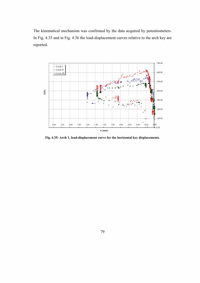
79

The kinematical mechanism was confirmed by the data acquired by potentiometers.

In Fig. 4.35 and in Fig. 4.36 the load-displacement curves relative to the arch key are

reported.

-700.00

-600.00

-500.00

-400.00

-300.00

-200.00

-100.00

0.00 0.00 0.20 0.400.600.801.001.201.401.601.80 2.002.202.40

w [mm]

F[N

]

Cycle I Cycle II Cycle III

Fig. 4.35: Arch 1, load-displacement curve for the horizontal key displacements.

80

-700.00

-600.00

-500.00

-400.00

-300.00

-200.00

-100.00

0.000.000.200.400.600.801.001.201.401.601.802.002.202.40

v [mm]

F [N

]

Cycle ICycle IICycle III

Fig. 4.36: Arch 1, load-displacement curve for the vertical key displacements.

A pushing action, characterized by a counter-clockwise spin and a vertical

displacement towards the bottom, was exercised by the block 1 on the arch. This

displacement was read by the potentiometer connected with the point in which the

load was applied. In Fig. 4.37 the load-displacement curves relative to the vertical

displacements of the point in which the load was applied are reported.

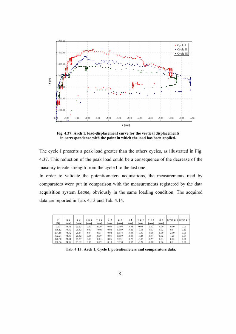
81

-700.00

-600.00

-500.00

-400.00

-300.00

-200.00

-100.00

0.00-6.50-6.00-5.50-5.00-4.50-4.00-3.50-3.00-2.50-2.00-1.50-1.00-0.500.00

v [mm]

F [N

]Cycle ICycle IICycle III

Fig. 4.37: Arch 1, load-displacement curve for the vertical displacements

in correspondence with the point in which the load has been applied.

The cycle I presents a peak load greater than the others cycles, as illustrated in Fig.

4.37. This reduction of the peak load could be a consequence of the decrease of the

masonry tensile strength from the cycle I to the last one.

In order to validate the potentiometers acquisitions, the measurements read by

comparators were put in comparison with the measurements registered by the data

acquisition system Leane, obviously in the same loading condition. The acquired

data are reported in Tab. 4.13 and Tab. 4.14.

F p_c c_c v_p_c v_c_c D_c p_f c_f v_p_f v_c_f D_f Error_p_c Error_p_f[N] [mm] [mm] [mm] [mm] [mm] [mm] [mm] [mm] [mm] [mm]0.00 74.73 25.53 0.00 0.00 0.00 53.04 19.35 0.00 0.00 0.00 0.00 0.00

196.12 74.70 25.52 -0.03 -0.01 0.02 52.89 19.22 -0.15 -0.13 0.02 0.67 0.13294.18 74.72 25.54 -0.01 0.01 0.02 52.74 19.05 -0.30 -0.30 0.00 2.00 0.00392.24 74.77 25.62 0.04 0.09 0.05 52.59 18.88 -0.45 -0.47 0.02 1.25 0.04490.30 74.81 25.67 0.08 0.14 0.06 52.51 18.78 -0.53 -0.57 0.04 0.75 0.08588.36 74.89 25.82 0.16 0.29 0.13 52.30 18.55 -0.74 -0.80 0.06 0.81 0.08

Tab. 4.13: Arch 1, Cycle I, potentiometers and comparators data.

82

F p_c c_c v_p_c v_c_c D_c p_f c_f v_p_f v_c_f D_f Error_p_c Error_p_f[N] [mm] [mm] [mm] [mm] [mm] [mm] [mm] [mm] [mm] [mm]

0.00 25.81 74.97 0.00 0.00 0.00 18.86 52.64 0.00 0.00 0.00 0.00 0.00137.28 25.81 74.97 0.00 0.00 0.00 18.76 52.57 -0.10 -0.07 0.03 0.00 0.30196.12 25.82 74.95 0.01 -0.02 0.03 18.60 52.41 -0.26 -0.23 0.03 3.00 0.12294.18 25.86 75.00 0.05 0.03 0.02 18.44 52.28 -0.42 -0.36 0.06 0.40 0.14392.24 25.96 75.05 0.15 0.08 0.07 18.07 51.95 -0.79 -0.69 0.10 0.47 0.13490.30 26.14 75.50 0.33 0.53 0.20 17.13 51.13 -1.73 -1.51 0.22 0.61 0.13

Tab. 4.14: Arch 1, cycle II, potentiometers and comparators data.

The errors in the displacements evaluation decreases with the increase of the

displacement values. The potentiometer under the arch key p_c makes an error

greater than the error made by potentiometer p_f because the achieved measurement

and the error of the instrument have the same order of magnitude.

83

4.12. Experimental campaign: Arch 2

Three loading-unloading cycles, called cycle I, II and III respectively, were carried

out applying the external load by the hydraulic jack connected with the brick number

14. The displacements were acquired by potentiometers and comparators; indeed the

applied load intensity was acquired by the small cell. Summarizing, the test

organization was the following:

cycle I: external load applied by the hydraulic jack;

cycle II: external load applied by the hydraulic jack;

cycle III: external load applied by the hydraulic jack.

Cycle I.

During this cycle the following hinges opening occurred:

hinge at the extrados between bricks 13-14, interface 14, in correspondence

of a load value equal to 400F N≅ ;

hinge at the intrados between bricks 7-8, interface 7, in correspondence of a


hinge at the extrados between bricks 1-2, interface 1, in correspondence of

a load value equal to 500F N≅ ;

hinge at the intrados between bricks 19-20, interface 20, in correspondence

of a load value equal to 550F N≅ .

84

Fig. 4.38: Arch 2, cycle I, experimental test.

Fig. 4.39: Arch 2, cycle I, hinges formation.

Cycle II and cycle III.

During the second and the third cycle the opening of the hinges occurred in

correspondence of an applied load lower than in the first cycle one. The peak load

decreased significantly from the value equal to 550PLF N≅ obtained in the first

cycle to a value equal to 450N obtained in the third cycle.


The hinges formation determined the arch subdivision in blocks. The collapse

mechanism occurred for relative displacements between the blocks. During the test

the same collapse mechanism, characterizing the Arch 1, occurred: the raising of the

second and third block, contrasting the pushing action towards the bottom.

85

4.12.2. Load-displacements curves

The load related to cycles I, II and III were acquired in continuous by the data

acquisition system Leane and the acquired data are reported in Fig. 4.40.

-700

-600

-500

-400

-300

-200

-100

00 240 480 720 960 1200 1440 1680 1920 2160 2400 2640 2880 3120

t [s]

F [N

]

Cycle I CycleIICycle III

Fig. 4.40: Arch 2, loading-unloading cycles.

In Fig. 4.41 and in Fig. 4.42 the load-displacement curves relative to the arch key are

reported.

86

-600

-500

-400

-300

-200

-100

0

100

0.000.200.400.600.801.001.201.401.601.802.00

w [mm]

F [N

]


Fig. 4.41: Arch 2, load-displacement curve for the horizontal key displacements.

-600

-500

-400

-300

-200

-100

0

100

0.000.200.400.600.801.00

v [mm]

F [N

]


Fig. 4.42: Arch 2, load-displacement curve for the vertical key displacements.

In Fig. 4.43 the load-displacement curves relative to the vertical displacements in the

point in which the load was applied are reported.

87

-630

-530

-430

-330

-230

-130

-30

70

-7.50-7.00-6.50-6.00-5.50-5.00-4.50-4.00-3.50-3.00-2.50-2.00-1.50-1.00-0.500.00

v [mm]

F [N

]

Cycle ICycleIICycle III

Fig. 4.43: Arch 2, load-displacement curve for the vertical displacements

in correspondence with the point in which the load has been applied.

Because of the decrease of the masonry tensile strength, the peak load of the cycle I

is greater than the one obtained in the others cycles, as illustrated in Fig. 4.43.

88

4.13. Experimental campaign: Reinforced arch

The experimental campaign on reinforced arches was performed only on the arch 2

because of the ominous collapse of the arch 1.

The instrumentations used for the experimental test on the reinforced arch was the

same used for the unreinforced arches.

4.13.1. Application of the FRP reinforcement

The FRP application was executed according to the codes (ACI 1999, fib TG 9.3

2001, JSCE 2001, etc.). The main phases of the reinforcement application were the

following:

Surface preparation: the surface where the reinforcement was applied was

suitable prepared. The arch surface was cleaned in order to remove every

imperfection present on it and every contamination of chemical nature.

Subsequently, it was necessary to fill the surface of the arch in order to

render it flat; when the FRP was applied on the arch surface, it was

completely clean, free from fats and oils and dry. At the end, the guides

lines to install the FRP were traced. In order to avoid that the epoxy resin

strewed over all the extrados surface, an adhesive tape was applied; it

delimited the field of reinforcement application (Fig. 4.44).

89

Fig. 4.44: Surface preparation.

Epoxy resin preparation: the epoxy resin was constituted by two

component; the first one, called A, was white and the other, called B, was

grey. Initially the two components were agitated separately, then they were

mixed according with the technical card. The mixture was good, and

therefore usable, when the colorful strips of the mixture were not more

visible. In Fig. 4.45 this process is illustrated.

Fig. 4.45: Epoxy resin preparation.

Epoxy resin application: the epoxy resin was applied on the arch surface

using a roller, as illustrated in Fig. 4.46.

90

Fig. 4.46: Epoxy resin application.

FRP application: the woven was measured and pre-cut before its application

on the arch surface. It was placed on the surface and gently pressed into the

epoxy resin, as illustrated in Fig. 4.47.

Fig. 4.47: FRP application.

Applying epoxy resin to FRP surface: a second coat of epoxy resin was

applied on the woven surface.

Consolidation process control: after 48 hours the applied reinforcement was

examined to verify the presence of empties.

91

4.13.2. Test organization

Three loading-unloading cycles, called cycle I, II and III respectively, were

performed applying the external load by the hydraulic jack in correspondence with

the brick number 14. The displacements were acquired by potentiometers and

comparators; the applied load intensity was acquired by the small cell during the first

cycle and by the great load cell in the other cases. Summarizing, the test organization

was the following:

cycle I: maximum external load applied 5000F N≅ ;

cycle II: maximum external load applied 25000F N≅ ;

cycle III: external load applied until the reinforced arch collapse.

Cycle I.

During this cycle the following phenomena occurred:

FRP delamination in correspondence of the mortar joint between bricks 13-

14 for a load value equal to 3000F N≅ , as illustrated in Fig. 4.48;

cracks under the brick 14, in correspondence of a load value equal to

3500F N≅ .

Fig. 4.48: Reinforced arch, cycle I, local delamination phenomenon at joint mortar.

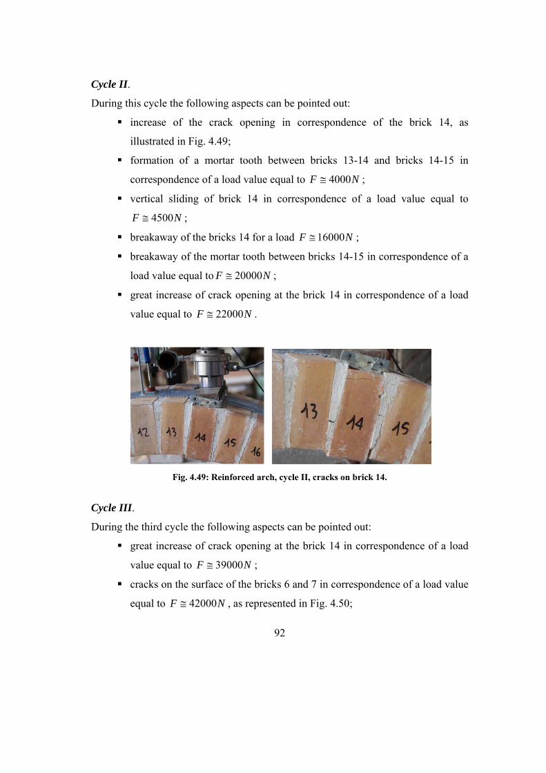
92

Cycle II.

During this cycle the following aspects can be pointed out:

increase of the crack opening in correspondence of the brick 14, as

illustrated in Fig. 4.49;

formation of a mortar tooth between bricks 13-14 and bricks 14-15 in

correspondence of a load value equal to 4000F N≅ ;

vertical sliding of brick 14 in correspondence of a load value equal to

4500F N≅ ;

breakaway of the bricks 14 for a load 16000F N≅ ;

breakaway of the mortar tooth between bricks 14-15 in correspondence of a


great increase of crack opening at the brick 14 in correspondence of a load

value equal to 22000F N≅ .

Fig. 4.49: Reinforced arch, cycle II, cracks on brick 14.

Cycle III.

During the third cycle the following aspects can be pointed out:

great increase of crack opening at the brick 14 in correspondence of a load

value equal to 39000F N≅ ;

cracks on the surface of the bricks 6 and 7 in correspondence of a load value

equal to 42000F N≅ , as represented in Fig. 4.50;

93

cracks on the surfaces of the bricks 8, 9, 10, 11 and 12 in correspondence of

a load equal to 50000F N≅ , as illustrated in Fig. 4.51;

collapse of the reinforced arch in correspondence with a load greater than

50000N , as represented in Fig. 4.52 and Fig. 4.53.

Fig. 4.50: Reinforced arch, cycle III, cracks formation on bricks surface.

Fig. 4.51: Reinforced arch, cycle III, intrados and extrados arch

surface view before the collapse.

94

Fig. 4.52: Reinforced arch, cycle III, arch collapse.

Fig. 4.53: Reinforced arch, after the collapse.

95


The reinforcement prevents the classic masonry arch collapse mechanism; the FRP

presence on the extrados surface, in fact, does not allow the hinges formation at the

intrados because it prevents the cracks opening at the extrados. During the tests, the

application of a concentrated load determined the presence of visible cracks on the

surface of the brick 14 in correspondence of a load value little than the load for

which the cracks on the other bricks occurred. The left part of the arch, from brick 1

to 14, was more significantly damaged than the right part of the arch, from brick 15

to 23. The collapse was preceded by the cracks opening on lateral and intrados

surfaces of all the bricks from 2 to 14. When the collapse occurred, the FRP

delamination under the bricks 13 and 14, the vertical sliding of the brick 14, the

crush of bricks from 8 to 13 and the partial crush of bricks from 2 to 7 took place.

4.13.4. Load-displacement curves

The data were acquired in continuous during the three loading-unloading cycles by

the data acquisition system Leane. The acquired data are reported in Fig. 4.54.

96

-60000

-55000

-50000

-45000

-40000

-35000

-30000

-25000

-20000

-15000

-10000

-5000

00 480 960 1440 1920 2400 2880 3360 3840 4320 4800 5280 5760

t [s]

F [N

]


Fig. 4.54: Reinforced arch, loading-unloading cycles.

The presence of the reinforcement induced an horizontal displacement in

correspondence of the arch key, that became more significant in proximity of the

collapse load. The load-displacement curves for the horizontal and the vertical key

displacements are reported in Fig. 4.55 and in Fig. 4.56, respectively; while in Fig.

4.57 the load-displacement curve for the vertical displacement connected with the

point of load application is reported.

97

-55000

-50000

-45000

-40000

-35000

-30000

-25000

-20000

-15000

-10000

-5000

0

5000

-2.0-1.5-1.0-0.50.00.51.01.52.02.53.03.54.04.55.05.56.0

w [mm]

F [N

]Cycle ICycle IICycle III

Fig. 4.55: Reinforced arch, load-displacement curve for the horizontal key displacement.

-55000

-50000

-45000

-40000

-35000

-30000

-25000

-20000

-15000

-10000

-5000

0

5000

-15-14-13-12-11-10-9-8-7-6-5-4-3-2-1012

v [mm]

F [N

]


Fig. 4.56: Reinforced arch, load-displacement curve for the vertical key displacement.

98

-55000

-50000

-45000

-40000

-35000

-30000

-25000

-20000

-15000

-10000

-5000

0

5000

-20-19-18-17-16-15-14-13-12-11-10-9-8-7-6-5-4-3-2-10

v [mm]

F [N

]


Fig. 4.57:Reinforced arch, load-displacement curve for the vertical displacements in

correspondence with the point in which the load has been applied.

During the test, the first loading-unloading cycle was characterized by arrangement

phase in which a push due to the bricks at extremities determined an horizontal

sliding of the arch; unfortunately it was not possible to measure it because there was

not the suitable instrumentation.

The presence of reinforcement has increased a lot the load-bearing of the arch, in

particular the arch strength is 100 times higher.

99

5. MODELING AND NUMERICAL PROCEDURES

5.1. Introduction

In this chapter the modeling and the numerical procedures developed to study the

behavior of unreinforced and reinforced masonry arches are presented. In particular,

two approaches able to solve nonlinear problems are illustrated: the first one is based

on the stress formulation and the second one is based on the displacement

formulation. In the stress formulation, the structural problem is faced and solved

developing a complementary energy approach. A numerical procedure, based on a

new formulation of the arc-length method, proposed by Riks in the framework of the

displacement approach [62], is developed. In the displacement approach, a three

nodes finite element based on the Timoshenko’s theory is implemented into FEAP

code [63]. The nonlinear problem is solved by the application of the finite element

method.

Moreover, a new post-computation technique of the stresses at the masonry-FRP

interface is proposed, which takes into account the heterogeneity of the masonry

material, responsible of local stress concentration. The proposed post-computation of

the FRP-masonry interface stresses is based on a simplified approach of the

multiscale method. In fact, once the stress analysis is performed on the homogenized

model of the arch, a micromechanical study is developed, considering the different

materials which constitute the masonry, i.e. the block, the mortar and the FRP

reinforcement.

Numerical applications are developed to assess the effectiveness of the proposed

models. Numerical results are put in comparison with the experimental results

available in the literature and with new experimental evidences obtained at the

100

LAPS. Moreover the unreinforced masonry arches numerical results are put in

comparison with those obtained by the application of the limit analysis.

5.2. Masonry constitutive models

The masonry material is modeled as a no-tension material with a limited compressive

strength. In particular, a nonlinear elastic constitutive relationship is considered for

the masonry material as the one proposed by Lucchesi et al. [36]. This approach is

simple and it can be considered effective for monotonic loading condition, when

local unloading does not occur in any point of the structure. When the loading cannot

be considered monotonic, the use of an elasto-plastic no-tension model is required, as

the one presented in Reference [18], where a model and a numerical procedure were

proposed and several numerical applications for reinforced masonry panels and

arches were developed. The structural behavior of the reinforced arch is determined

developing a variational formulation based on the complementary energy, i.e.

adopting a stress approach. In fact, for the analysis of elements made of no-tension

material, the solution of the structural problem, if it exists, is unique in terms of

stress, while it could be not unique in terms of displacements, as proved by Lucchesi

et al. [36].

5.2.1. Model 1

The masonry material is modeled as a masonry like material, assuming a behavior

characterized by no-tension response with limited strength in compression, Fig. 5.1.

The lack of tensile response gives an admissibility condition for stresses:

0Mσ ≤ (5.1)

101

The condition 0Mσ = can be defined as a limit or collapse condition and in this case

the strains have an indefinite non negative value.

The compression strength is denoted as σy. The adopted model is simple, but very

effective for a wide class of problems, as emphasized in literature.

Fig. 5.1: Masonry constitutive model, model 1.

In Fig. 5.1 it can be individuated the following features:

feature OD: linear elastic;

feature DE: ideal plastic.

In terms of deformations, there are three distinctive features:

feature OD: elastic reversible strain;

feature DE: inelastic irreversible strain;

point E: yield strain.

It is assumed the existence of the following form for the complementary energy

density governing the stress-strain relationship:

( ) ( ) ( )( )2 21 1, 12 2M M M M M M

M M

I hE G

ψ σ τ σ σ τ σΣ= + + − (5.2)

ε

σM

σy

εy

O

D E

102

where EM and GM are the elastic and the shear modulus of masonry respectively, IΣ

is the indicator function of the admissible set ,0yσ⎡ ⎤Σ = ⎣ ⎦ , assuming the following

values:

0 if

otherwiseMI

IσΣ

Σ

= ∈Σ= +∞

(5.3)

and ( )Mh σ is the Heaviside’s function, assuming the following values:

( )( )

1 if 0

0 otherwiseM M

M

h

h

σ σ

σ

= ≥

= (5.4)

Fig. 5.2: Masonry complementary energy density.

σM

ψ

103

As consequence of the existence of the potential (5.2), that is schematized in Fig. 5.2,

the normal and tangential stresses, σ M and τ M , do not depend on the specific strain

history and they can be determined by the formulas:

0if 0

0

if 0

if

M

M

M My

M M

M M yy

M M

EG

E

G

σε

τ

σ εε ε

τ γ

σ εε ε

τ γ

= ⎫>⎬= ⎭

= ⎫< ≤⎬= ⎭

= ⎫⎪ ≤⎬= ⎪⎭

(5.5)

where /y y MEε σ= is the limit strain in compression and yσ is the compressive

strength. A simple shear stress-strain behavior is assumed; in fact, it is nonlinear

elastic in the part of the cross-section in compression. In this way the possible

collapse due to shear sliding cannot be reproduced.

5.2.2. Model 2

In order to improve the model previously presented, it is considered a constitutive

law characterized, for small values of the strain, by a quadratic relationship between

the stress and the strain, as the one proposed for the concrete by the Eurocode 2.

Thus, for yε ε≤ , the stress-strain relationship is:

2Mσ αε βε μ= + + (5.6)

The following conditions are imposed on the relationship (5.6):

104

0 , 00 , '

,, ' 0

M

M

y M y

y M

Eε σε σε ε σ σε ε σ

= == == == =

(5.7)

Solving equations (5.7) with respect to α , β , μ and yε , it results:

2

2 20y y y

yy y E

σ σ σα β μ ε

ε ε= − = = = (5.8)

Substituting solution (5.8) into the equation (5.6):

22 for 0y

M yy

Eσ

σ ε ε ε εε

= − + ≤ ≤ (5.9)

Finally, the normal and tangential masonry stresses, σ M and τ M , can be determined

by the formulas:

2

0if 0

0

)if 0

if

M

M

My

M M

M yy

M M

G

G

σε

τ

σ αε βεε ε

τ γ

σ σε ε

τ γ

= ⎫>⎬= ⎭

⎫= + ⎪ < ≤⎬= ⎪⎭= ⎫⎪ ≤⎬= ⎪⎭

(5.10)

in which and α β assume the values reported in expressions (5.8).

Also in this case the possible collapse due to shear sliding cannot be captured. The

constitutive relationship is schematically illustrated in Fig. 5.3.

105

Fig. 5.3: Masonry constitutive model, Model 2.

5.3. FRP constitutive model

Design of FRP reinforcement should ensure that the FRP system is always in tension.

In fact, compression FRP is unable to increase the performance of the strengthened

masonry member due to its small area compared to that of compressed masonry.

Moreover, FRP in compression may be subjected to debonding due to local

instability.

A uniaxial linear elastic response is assumed for the FRP reinforcement, as illustrated

in Fig. 5.4.

ε

σM

σy

εy

O

εu

106

Fig. 5.4: FRP constitutive model.

The stress-strain relationship is:

R REσ ε= (5.11)

where ER is the elastic modulus of the FRP reinforcement. The corresponding

complementary energy is:

( ) 212R R R

REψ σ σ= (5.12)

σ

ε

brittle failure

107

5.4. Limit analysis

In this section a brief discussion both on the plastic collapse theorems and limit

analysis is presented.

Numerous studies have been made on the theory of plasticity since the Hill’s [64],

[65] and Prager’s and Hodge’s [66] works.

The aim of the limit analysis is to evaluate the load capacity and the collapse

mechanism of structures. Considering the limit behavior of the material, through a

definition of a yield function ϕ in terms of stresses, it is assumed that if 0ϕ < the

material remains in the elastic phase, if 0ϕ = the material becomes plastic and if

0ϕ > the stress state is inadmissible. The set 0ϕ = is called the yield surface and

the conditions 0ϕ ≤ represent the admissible stresses. According to the definition of

ϕ , all points that are inside or on the yield surface are admissible, while all points

located outside the yield surface are inadmissible. When the stress state belong to the

yield surface and the plastic behavior is activated, it is necessary to define the flow

direction. According to the classical limit analysis theory [67], the yield surface is

convex and the flow direction is normal to the yield surface. The normality condition

assures that the energy dissipated by the flow is the maximum possible. The

normality condition is very important because it introduces great simplifications in

the limit analysis theory and it is the base of the limit analysis theorems.

For a structure, it is possible to define a statically admissible state (safe state) for

which the internal stresses are in equilibrium with the external forces and the yield

conditions are fulfilled in all the points. Making a proportional loading analysis, it is

necessary to define q , that is the base variable load, λ , the definite positive load

factor and λq , the variable load applied on the structure. The applied load can be

increased from zero until a limit value for the structure, through the use of the load

factor. This limit value is called the safety factor. In the limit analysis theory, the

108

static and kinematical theorems are proved; moreover, the uniqueness theorem can

be also proved.

The static theorem, also called lower-bound theorem, affirms that the safety factor is

the largest of all statically admissible load factors. In other words, if it is possible to

find a statically admissible stress field for a given load factor. Consequently the

structure is in a safe condition under that load level.

The kinematical theorem, also called upper-bound theorem, ensures that the safety

factor is the smallest of all the kinematically admissible load factors.

Finally, for the uniqueness theorem the largest factor defined by the static theorem is

equal to the smallest factor defined by the kinematical theorem.

The use of those fundamental theorems requires the adoption of specific hypotheses,

particularly for masonry structures. Among these, the non tensile strength, the

infinite compressive strength, the absence of sliding failure and the small

displacements.

In the following the kinematical theorem is applied to the case of unreinforced

masonry structures considering the no-tensile strength of the masonry.

109

5.5. Arch model

The arch model is based on the theory of curvilinear beam. Several shear

deformation beam theories are available in literature. In the following the

Timoshenko’s beam theory, [68] and [69], is considered; it is widely used in

structural analysis, as it accounts for the transverse shear deformation in a simple and

effective manner.

The compatibility, the equilibrium and the constitutive equations governing the

problem of the arch are available in literature; herein, only the final results are

reported.

Two coordinate systems are introduced: a global system (O, x, y, z) and a local

system (x*, y*, z*), with x* and y* rotated of an angle θ with respect to y, as

schematically illustrated in Fig. 5.5.

Fig. 5.5: Arch global and local systems.

A typical infinitesimal part of the arch is reported in Fig. 5.6. The quantities in the

local coordinate system are computed as function of the ones represented in the

global system using a rotation matrix R. The local radius of the arch is indicated as

R, while s denotes the curvilinear abscissa.

110

Fig. 5.6: Infinitesimal arch element.

5.5.1. Governing equation of the arch

The arch is assumed subjected to a permanent and to a variable loading p and λq ,

respectively, with λ the load multiplier. Thus, the equilibrium equations written in

the local coordinate system take the form:

λ+ + =* *Δc p q 0 (5.13)

where

* *

* *

* *

10

0 1 0 0

1 0

s s

r r

dds R p qN

d Mds

T p qdR ds

⎡ ⎤⎢ ⎥

⎧ ⎫ ⎧ ⎫⎧ ⎫⎢ ⎥⎪ ⎪ ⎪ ⎪⎪ ⎪⎢ ⎥= − = = =⎨ ⎬ ⎨ ⎬ ⎨ ⎬⎢ ⎥ ⎪ ⎪ ⎪ ⎪ ⎪ ⎪⎢ ⎥ ⎩ ⎭ ⎩ ⎭ ⎩ ⎭⎢ ⎥−

⎢ ⎥⎣ ⎦

Δ c p q

N+dN

N

T M

T+dT

M+dM

s

dθ

p*

q*

y* z*

y

z O

111

with N, M and T the stress resultants and ps*, qs

* and pr*, qr

* the tangential and radial

distributed components of the loads. Note that *p and λ *q are the permanent and

variable loads vectors represented in the local coordinate system.

5.5.2. Kinematics of the arch

The kinematics of the typical cross section of the arch is defined by the transversal

and the axial displacements, v* and w0* respectively, and by the rotation ϕ. The

compatibility equations are:

=*Δη d% (5.14)

where

*0 0

*

*

10

0 0

1 1

dds R w

dds

vdR ds

εϕ χ

γ

⎡ ⎤⎢ ⎥

⎧ ⎫ ⎧ ⎫⎢ ⎥⎪ ⎪ ⎪ ⎪⎢ ⎥= = =⎨ ⎬ ⎨ ⎬⎢ ⎥ ⎪ ⎪ ⎪ ⎪⎢ ⎥ ⎩ ⎭⎩ ⎭⎢ ⎥−

⎢ ⎥⎣ ⎦

Δ η d%

in which γ representing the shear deformation, ε0 the axial strain and χ the bending

curvature.

5.5.3. Cross section

The cross sections of the arches typically present very regular geometry; thus,

without loosing in generality, a rectangular cross section is considered in the

112

following. In accordance with the local coordinate system introduced above, the

section lies in the x*y* plane, with x* and y* principal inertial axes.

In the determination of the overall behavior of the reinforced masonry arch section, a

perfect adhesion between masonry and FRP is assumed.

The strain at a point of the section is:

*0 yε ε χ= + (5.15)

The section AM of the masonry is split in three parts:

the no-reagent part for which 0ε > , denoted as Ant;

the compressed part for which 0yε ε< ≤ , denoted as Ae;

the compressed part subjected to a constant stress for which yε ε≤ , denoted

as Ap.

In order to determine the parts Ant, Ae and Ap, the neutral and the plasticity axes * *

ny y= and * *my y= , for which the strain attains the values zero and yε ,

respectively, are determined:

* * 00

0* *0

0 n n

yy m m

y y

y y

εε χχ

ε εε ε χ

χ

= + ⇒ = −

−= + ⇒ =

(5.16)

Two possible cases can occur, schematically illustrated in Fig. 5.7, depending on the

sign of the curvature.

113

Fig. 5.7: Axes position for positive and negative curvature.

The axes defining the compressed parts of cross section are determined as:

1

1 3 *2

3 2

*3

0

2:

min ,max ,: 2 2

min ,max ,2 2

pn

e

m

hy

A y y y h hy yA y y y

h hy y

χ ≥

⎧⎪ = −⎪⎪≤ ≤ ⎧ ⎫⎪ ⎧ ⎫= −⎨ ⎨ ⎨ ⎬⎬< ≤ ⎩ ⎭⎩ ⎭⎪⎪ ⎧ ⎫⎧ ⎫⎪ = −⎨ ⎨ ⎬⎬⎪ ⎩ ⎭⎩ ⎭⎩

(5.17)

*1

3 22

1 3

*3

0

min ,max ,2 2

:2:

min ,max ,2 2

n

p

e

m

h hy y

A y y y hyA y y y

h hy y

χ <

⎧ ⎧ ⎫⎧ ⎫= −⎨ ⎨ ⎬⎬⎪⎩ ⎭⎩ ⎭⎪

≤ ≤ ⎪⎪ =⎨≤ < ⎪

⎪ ⎧ ⎫⎧ ⎫= −⎨ ⎨ ⎬⎬⎪⎩ ⎭⎩ ⎭⎪⎩

(5.18)

AFRP AFRP

114

5.6. Stress formulation

In this section only the Model 1 is considered for masonry. Thus the section AM of

the masonry is specialized into:

Ant where 0ε > and, as consequence of equations (5.5), 0 0M Mσ τ= = ;

Ae where 0yε ε< ≤ and, as consequence of equations (5.5),

M M M ME Gσ ε τ γ= = ; in the compressed part of the cross-section,

characterized by a linear stress-strain relation, the normal stress is

represented as *0 1M yσ σ σ= + ;

Ap where yε ε≤ and M M y M ME Gσ ε τ γ= = .

The resultants in the reinforced masonry are:

( )

( )

*0 1

* * *0 1

ˆ

p e

p e

e p

y RA A

y RA A

MA A

dA y dA N

NM y dA y y dA M

TT

dA

σ σ σ

σ σ σ

τ∪

⎧ ⎫⎪ ⎪+ + +⎪ ⎪⎪ ⎪⎧ ⎫

⎧ ⎫ ⎪ ⎪ ⎪ ⎪= = = + + +⎨ ⎬ ⎨ ⎬ ⎨ ⎬⎩ ⎭ ⎪ ⎪ ⎪ ⎪

⎩ ⎭ ⎪ ⎪⎪ ⎪⎪ ⎪⎩ ⎭

∫ ∫

∫ ∫

∫

cc (5.19)

Developed, the formulas (5.19) become:

0 1

0 1

y p e e R

y p e e R

M S

A A S NS S I MA

σ σ σσ σ στ

+ + +⎧ ⎫⎪ ⎪= + + +⎨ ⎬⎪ ⎪⎩ ⎭

c (5.20)

where ( )S T e pA A Aχ= + is the shear area, Tχ is the shear correction factor, Se and Sp

are the static moments of elastic and plastic part, respectively, Ie is the inertial

moment of elastic part, NR and MR are the stress resultants due to the reinforcement.

115

Because of the perfect adhesion between the masonry arch and the reinforcement, the

resultants of the stresses at the top ( * / 2y h= − ) and the bottom ( * / 2y h= )

reinforcements are expressed as:

0 0 1

0 0 1

2

2

R R

R R

hN n A

hN n A

σ σ

σ σ

+ +

− −

⎛ ⎞= −⎜ ⎟⎝ ⎠⎛ ⎞= +⎜ ⎟⎝ ⎠

(5.21)

with 0 /R Mn E E= the homogenization coefficient; so that the resultants of the

reinforcements are:

( )( )

0 0 1

0 0 1

R R R

R R R

N n A S

M n S I

σ σ

σ σ

= +

= + (5.22)

where

( )( ) ( )2

/ 2

/ 2

R R R

R R R

R R R

A A A

S h A A

I h A A

+ −

+ −

+ −

= +

= −

= +

(5.23)

Formulas (5.23) represent the area, the static and the moment of inertia, respectively,

of the FRP.

It can be emphasized that the parts Ant, Ae and Ap are not known a priori, but they

have to be determined as functions of the kinematical quantities ε0 and χ.

Setting:

116

0

1

0

, , ,

,

py

p

e e R R

e e R R

AS

A S A Sn

S I S I

σσ

σ⎧ ⎫⎧ ⎫

= = = +⎨ ⎬ ⎨ ⎬⎩ ⎭ ⎩ ⎭

⎡ ⎤ ⎡ ⎤= =⎢ ⎥ ⎢ ⎥

⎣ ⎦⎣ ⎦

σ Q J J J

J J

)%

)%

(5.24)

from expression (5.20), taking into account equations (5.22), the values of 0σ and

1σ are obtained as:

( )ˆ= −σ H c Q (5.25)

where 1−=H J .

It can be emphasized that, because of expression (5.25), the stress in the masonry as

well as the stress in the reinforcement can be expressed as function of the stress

resultants N and M. In particular, the stress in the elastic part of the masonry section

and on the reinforcements is determined as:

( )( )( )

0

0

ˆ

ˆ

ˆ

M

R R

R R

N n A

N n A

σ+ + +

− − −

= − •

= − •

= − •

H c Q Y

H c Q Y

H c Q Y

(5.26)

where *1T

y=Y , 1 / 2 Th+ =Y and 1 / 2 Th− = −Y , while the symbol •

indicates the scalar product.

117

5.6.1. Complementary energy

In this section the elastic problem is faced and solved developing an energy

approach. The complementary energy of the structure is defined as:

( ) ( ) ( )

2 2 2

, ,

2 2 2

M R

M R

M RV V

M M RV V

dV dV

dV dVE G E

σ τ ψ σ τ ψ σ

σ τ σ

Ψ = +

⎛ ⎞= + +⎜ ⎟

⎝ ⎠

∫ ∫

∫ ∫ (5.27)

where VM and VR are the masonry and the reinforcement volume, respectively. In

particular, the complementary energy in the masonry and in the reinforcement

domains can be written in the form:

( )

( ) ( )

2 2

2

2 2

12

,1

2

1 ˆ ˆ2

2 2

f

e p

M i

e p

f

i

M yM A A

M M MV

MM A A

M

y p S

M M S

dA dAE

dV R d

dAG

ER d

A TE G A

θ

θ

θ

θ

σ σψ σ τ θ

τ

θσ

∪

⎡ ⎤⎛ ⎞⎢ ⎥⎜ ⎟+

⎜ ⎟⎢ ⎥⎝ ⎠= ⎢ ⎥⎢ ⎥+⎢ ⎥⎣ ⎦⎡ ⎤− ⊗ − •⎢ ⎥⎢ ⎥=⎢ ⎥+ +⎢ ⎥

⎢ ⎥⎣ ⎦

∫ ∫∫ ∫

∫

∫H c Q H c Q J%

(5.28)

( )

( ) ( )

2

0

12

ˆ ˆ2

f

R i R

f

i

R R RRV A

R

dV dA dsE

n R dE

θ

θ

θ

θ

ψ σ σ

θ

=

= − ⊗ − •

∫ ∫ ∫

∫ H c Q H c Q J)

(5.29)

118

with iθ and fθ the angles defining the initial and the final section of the arch.

Finally, the complementary energy is obtained as:

( )( ) ( )

2

2

1 ˆ ˆ2 2ˆ,

2

f

i

y p

M M

M S

AE E

T R dT

G A

θ

θ

σ

θ

⎡ ⎤− ⊗ − • +⎢ ⎥

⎢ ⎥Ψ = ⎢ ⎥⎢ ⎥+⎢ ⎥⎣ ⎦

∫H c Q H c Q J

c (5.30)

The solution of the problem is determined minimizing the complementary energy

(5.30) under the equilibrium constraint. In fact, the equilibrated stress resultants

admit the following representation form:

1

1

1

1

1

1

ˆ ˆ ˆ

p q

h

p q i ii

h

p q i ihi

p q i i hi

p q i ihi

p q i i hi

i ii

x

N N x Nx

M M x MT T x T

T T x T

λ

λλ

λλ

λ

=

=

=

=

=

=

= + +

⎧ ⎫+ +⎪ ⎪⎧ ⎫ ⎪ ⎪+ +⎪ ⎪ ⎪ ⎪⎪ ⎪= = + +⎨ ⎬ ⎨ ⎬

⎪ ⎪ ⎪ ⎪+ +⎪ ⎪ ⎪ ⎪⎩ ⎭ + +⎪ ⎪

⎩ ⎭

∑

∑∑

∑∑

∑

c c c c

c c c (5.31)

with pc a field of stress resultants equilibrated with permanent loads p, qc a field of

stress resultants equilibrated with variable loads q, ic with i=1,..,h fields of self-

equilibrated stress resultants and xi with i=1,..,h statically unknown parameters. The

number h of self-equilibrated stresses depends on the structural system and on the

constraint conditions.

Substituting the representation form (5.31) into the complementary energy (5.30), the

stationary condition of complementary energy with respect to the unknown minimum

119

parameters x1, x2,.., xh is enforced in order to solve the elastic problem. The typical

stationary equation takes the form:

1

1

1 ˆ ˆ ˆ ˆ

0f

i

h

p q i i jiM

h

j j p q i ii

M S

xE

R dx T T T x T

G A

θ

θ

λ

θλ

=

=

⎡ ⎤⎛ ⎞⎛ ⎞+ + − •⎢ ⎥⎜ ⎟⎜ ⎟

⎝ ⎠⎝ ⎠⎢ ⎥∂Ψ ⎢ ⎥= = ⎛ ⎞∂ ⎢ ⎥+ +⎜ ⎟⎢ ⎥⎝ ⎠+⎢ ⎥⎣ ⎦

∑

∫ ∑

H c c c Q c

(5.32)

which correspond to a kinematical compatibility equation. In fact, denoting as:

1 ˆ ˆ

1 ˆ ˆ

1 ˆ ˆ

1 ˆ

f

i

f

i

f

i

f

i

j pp p j

M M S

j qq q j

M M S

j ii i j

M M S

Q jM

T TR d

E G A

T TR d

E G A

T TR d

E G A

R dE

θ

θ

θ

θ

θ

θ

θ

θ

θ

θ

θ

θ

⎛ ⎞= • +⎜ ⎟

⎝ ⎠

⎛ ⎞= • +⎜ ⎟

⎝ ⎠

⎛ ⎞= • +⎜ ⎟

⎝ ⎠

= •

∫

∫

∫

∫

s H c c

s Hc c

s Hc c

s Q c

(5.33)

the compatibility equation (5.32) takes the form:

1

h

p q i i Qi

xλ=

+ + − =∑s s s s 0 (5.34)

where , ,p q is s s and Qs are vectors of h components which assume the physical

meaning of the displacement associated to the permanent and variable loadings p and

120

q, to the self-equilibrated stress resultants ic and to the additive stresses due to the

inelastic behavior of the masonry material.

It can be emphasized that, because of the considered nonlinear constitutive laws, the

vectors , ,p q is s s and Qs depend on the solution, in fact they depend on the partition

of the section AM of the masonry into the no-reagent part Ant, the elastic part Ae and

the plastic part Ap, i.e. ( ),p p e pA A=s s , ( ),q q e pA A=s s , ( ),i i e pA A=s s and

( ),Q Q e pA A=s s .

The integration of equations (5.32) and (5.33) can be performed considering the arch

composed of a number of nT parts in each of which the positions of the axes defined

by y1, y2 and y3 are taken constant.

5.6.2. Arc-length technique

The considered constitutive law for the masonry material, characterized by limited

strength in compression with no-tensile response, leads to solve a nonlinear problem

governed by equation (5.32). It could be remarked that, because of the elastic

character of the constitutive equations for both the masonry and the reinforcement,

the solution of the structural problem does not depend on the loading history, so that

the stress state can be computed once the loading is assigned. Although the

constitutive equations are not written in evolutive form, a numerical procedure able

to solve the nonlinear problem (5.32) is developed considering the loading applied in

several steps. In such a way, each loading step results easier to solve and, moreover,

it is possible to define the behavior of the structure along the whole monotone

loading path. In this context, the compatibility equation (5.34) can be written in the

form:

121

( ) ( ) ( )

( ) ( ) ( ),1

, ,

, ,

p e p n q e p

h

i n i i e p Q e pi

A A A A

x x A A A A

λ λ

=

= + + Δ +

+ + Δ − =∑

s s s

s s 0 (5.35)

Furthermore, it is possible to define a limit load for the structure, i.e. a load

multiplier λ which induces the collapse of the arch. In order to evaluate the whole

nonlinear structural response of the arch and to compute the limit load, the arc-length

technique is considered.

The arc-length procedure is often developed in the framework of displacement or

mixed formulation of the structural problem. In the following, a new version of the

arc-length technique, based on the stress formulation, is proposed. In particular, the

developed arc-length procedure is based on the kinematical compatibility equation

(5.35) and on a constraint equation.

The nonlinear equation (5.35) is solved developing an iterative procedure within

each load step. Thus, denoting by the superscript k the solution at the k-th iteration,

the new solution is determined developing equation (5.35) in Taylor series:

1 kk

hk

ii i

k k k

xx

δ δλλ

δ δλ

= ==

∂ ∂= + +

∂ ∂

= + + =

∑s ss s

s ss s

s K x S 0

(5.36)

where

122

( ) ( ) ( )( ) ( ) ( ),

1

1 1 1

1

1

, ,

, ,

...

. . .

. .... . .

. .

....

k k k

kk k

k k k k k kp e p n q e p

hk k k k k

i n i i e p Q e pi

h

k k

hh h

h

A A A A

x x A A A A

s s sx x

ss sx x

λ λ

λ

λ

=

= = =

== =

= + + Δ

+ + Δ −

⎡ ⎤∂ ∂ ⎧ ⎫∂⎢ ⎥ ⎪ ⎪∂ ∂ ∂⎢ ⎥ ⎪ ⎪⎢ ⎥ ⎪ ⎪⎢ ⎥ ⎪ ⎪

= =⎢ ⎥ ⎨ ⎬⎢ ⎥ ⎪ ⎪⎢ ⎥ ⎪ ⎪⎢ ⎥ ⎪ ⎪∂∂ ∂⎢ ⎥ ⎪ ⎪∂∂ ∂ ⎩ ⎭⎢ ⎥⎣ ⎦

∑

s s s s s s

s ss s s s

s s s

s s

K S

(5.37)

The new solution is determined solving equation (5.36):

( ) ( )1 1k k k k k k ktδ δλ δ δ δλ

− −= − − = +x K s K S x x (5.38)

so that the variation of statically unknown parameters results:

k k k k ktδ δ δ δλΔ = Δ + = Δ + +x x x x x x (5.39)

The updating of the geometrical quantities eA and pA is performed computing the

neutral and the plasticity axes, solving equation (5.16), and then (5.17) or (5.18).

Note that the kinematical parameters present in formulas (5.16) are evaluated solving

the resultant constitutive equations in a typical section of the arch:

00

k kk kR Re e

M k kk kR Re e

A SA SNE n

S IS IMεχ

⎛ ⎞⎡ ⎤⎧ ⎫ ⎧ ⎫⎡ ⎤= +⎜ ⎟⎨ ⎬ ⎨ ⎬⎢ ⎥ ⎢ ⎥⎜ ⎟⎣ ⎦⎩ ⎭ ⎩ ⎭⎣ ⎦⎝ ⎠

(5.40)

123

The constraint equation required in the arc-length method is defined choosing a

suitable control parameter. In particular, it is assumed as control parameter the

maximum variation of bending curvature evaluated on all the cross sections of the

arch. Thus, it is set:

( )maxi fθ θ θ

χ χ θ≤ ≤

= Δ% (5.41)

and the constraint equation is assumed of the form:

2 2 0lχ − Δ =% (5.42)

where lΔ is a given length of the radius considered to follow the mechanical

response path of the structure.

For a fixed value of the angle θ , i.e. in the typical cross-section, solving equation

(5.40) with definition (5.41), it is set:

( )

2

212 1 2

221

+/

+

q

q

hk

i ii

Mh

i ii

H N x NE

H M x M

λχ

λ

=

=

⎡ ⎤⎛ ⎞Δ Δ⎢ ⎥⎜ ⎟

⎝ ⎠⎢ ⎥=⎢ ⎥⎛ ⎞+ Δ Δ⎢ ⎥⎜ ⎟⎢ ⎥⎝ ⎠⎣ ⎦

∑

∑% (5.43)

On the other hand, as it is kλ λ δλΔ = Δ + , equation (5.43) becomes:

( ) ( ) ( ) ( ) ( )

( )( )

2 22 2 221 22

21 222

k k

k k

H n n H m m

H H n n m mλ λ

λ λ

χ δλ δλ

δλ δλ

= + + +

+ + +

% (5.44)

where:

124

( )

( )1

1

,1

,1

+

+

q

q

q

q

hk k k

i i ii

hk k k

i i ii

hk

t i ii

hk

t i ii

n x x N N

m x x M M

n N x N

m M x M

λ

λ

δ λ

δ λ

δ

δ

=

=

=

=

= Δ + + Δ

= Δ + + Δ

=

=

∑

∑

∑

∑

(5.45)

Equation (5.42), taking into account formula (5.44), can be written in the form:

21 2 3 0a a aδλ δλ+ + = (5.46)

where:

( ) ( )( ) ( )

( ) ( )

2 22 21 21 22 21 22

2 2

2 21 22 21 22

21 222 22 2 2

3 21 22 21 22

2

2 2 +2

2

2

k k k k

k k k k

k k

k k k k

a n H m H n m H H

a n n H m m H n m H H

n m H H

a H n H m n m H H l

λ λ λ λ

λ λ λ

λ

= + +

= +

+

= + + − Δ

(5.47)

Equation (5.46) is solved with respect to δλ , leading to the determination of two

roots, 1δλ and 2δλ . The solution is chosen according to the cylindrical method, such

that 2δλ δλ= if 2 1c c> and it is 1δλ δλ= otherwise, with

125

( )41

51

1 4 5 1

2 4 5 2

hk k k

i i iih

k ki i

i

a x x x

a x x

c a ac a a

δ

δ

δλδλ

=

=

= Δ + Δ

= Δ

= +

= +

∑

∑ (5.48)

The load multiplier and the statically unknown parameters increments are updated

setting:

k

k k k kt

λ λ δλ

δ δ δλ δ

Δ = Δ +

Δ = Δ + = Δ + +x x x x x x (5.49)

The iteration process within each loading step is performed until the residual r = s

is greater than a fixed tolerance.

5.7. Displacement formulation

The displacement formulation approach has been developed considering both Model

1 and Model 2. In this section, only the Model 2 is described.

The section AM of the masonry is specialized into:

Ant where 0ε > and, as consequence of equations (5.10), 0 0M Mσ τ= = ;

Ae where 0yε ε< ≤ and, as consequence of equations (5.10),

2M M MGσ αε βε τ γ= + = ;

Ap where yε ε≤ and M y M MGσ σ τ γ= = .

The resultants in the reinforced masonry are:

126

2

* * 2

( )

ˆ ( )

p e

p e

e p

y RA A

y RA A

MA A

dA dA N

NM y dA y dA M

TT

dA

σ αε βε

σ αε βε

τ∪

⎧ ⎫⎪ ⎪+ + +⎪ ⎪⎪ ⎪⎧ ⎫

⎧ ⎫ ⎪ ⎪ ⎪ ⎪= = = + + +⎨ ⎬ ⎨ ⎬ ⎨ ⎬⎩ ⎭ ⎪ ⎪ ⎪ ⎪

⎩ ⎭ ⎪ ⎪⎪ ⎪⎪ ⎪⎩ ⎭

∫ ∫

∫ ∫

∫

cc (5.50)

The axial resultant and bending moment are computed as:

( ) ( )

2

2* *0 0

0

( )

p e

e

y RA A

y p RA

y p R

N dA dA N

A y y dA N

A A S N

σ αε βε

σ α ε χ β ε χ

σ ε χ

= + + +

⎡ ⎤= + + + + +⎢ ⎥⎣ ⎦

= + + +

∫ ∫

∫% %

(5.51)

( ) ( )

* * 2

2* * *0 0

0

( )

p e

e

y RA A

y p RA

y p R

M y dA y dA M

S y y y dA M

S S I M

σ αε βε

σ α ε χ β ε χ

σ ε χ

= + + +

⎡ ⎤= + + + + +⎢ ⎥⎣ ⎦

= + + +

∫ ∫

∫% %

(5.52)

respectively, where

( ) ( )*0 0

e

e eA

A y dA A Sαε α χ β αε β αχ= + + = + +∫% (5.53)

( ) ( )* *2 *0 02

e

e eA

S y y y dA S Iαε α β αε β αχ= + + = + +∫% (5.54)

127

( ) ( )*3 *2 *20 0

e

eA

I y y y dA I Iα χ β αε αε β αχ= + + = + +∫)

% (5.55)

and ( )S T e pA A Aχ= + is the shear area, Tχ is the shear correction factor, NR and MR

are the stress resultants due to the reinforcement.

5.7.1. Kinematics

The kinematics of the Timoshenko beam theory, schematically illustrated in Fig. 5.8,

can be expressed as

1

2

3

0uu vu w yϕ

=== +

(5.56)

Fig. 5.8: Timoshenko’s beam theory.

The strain field is given by

0 '

''

w

v

εχ ϕγ ϕ

=

== +

(5.57)

128

Note that the prime on a variable indicates its derivative with respect to z . The

kinematics strain vector is introduced as

0

0 0'' 0 0

'0 1

ddzw w w

d v vdz

v ddz

εχ ϕγ ϕ ϕ ϕ

⎛ ⎞⎜ ⎟

⎧ ⎫ ⎧ ⎫ ⎧ ⎫ ⎧ ⎫⎜ ⎟⎪ ⎪ ⎪ ⎪ ⎪ ⎪ ⎪ ⎪⎜ ⎟= = = =⎨ ⎬ ⎨ ⎬ ⎨ ⎬ ⎨ ⎬⎜ ⎟⎪ ⎪ ⎪ ⎪ ⎪ ⎪ ⎪ ⎪+ ⎜ ⎟⎩ ⎭ ⎩ ⎭ ⎩ ⎭ ⎩ ⎭

⎜ ⎟⎜ ⎟⎝ ⎠

d L (5.58)

5.7.2. Finite element implementation

A discussion on displacement based or mixed formulation beam elements was

presented by Crisfield [70], [71]. Reddy, [72]-[74], developed superconvergent (i.e. ,

yields exact nodal values) locking-free Timoshenko’s beam finite element based on

the interdependent interpolation as well as assumed strain formulation. In the same

paper, Reddy extended the procedure to develop a locking-free finite element for the

third-order beam theory. A consistent beam finite element was proposed in reference

[75].

The conventional finite element model of the Timoshenko’s beam is obtained by

using Lagrange interpolation of v and ϕ . For example, linear interpolation of both

v and ϕ is known to yield a finite element that exhibits locking. Reduced integration

of the shear stiffness alleviates this problem, but does not yield exact values of the

displacements at the nodes without using a large number of elements. Here, we

consider an alternative interpolation of the dependent variables that yields a locking-

free finite element. In particular, the transverse displacement v is approximated

using the Hermite’s cubic interpolation, the rotation ϕ and the axial displacement w

are approximated using Lagrange quadratic interpolation:

129

1 1 2 2 3 3

1 1 2 2 1 1 2 2

1 1 2 2 3 3

w w w

v v

w N w N w N w

v N v N v N N

N N N

θ θ

ϕ ϕ ϕ

θ θ

ϕ ϕ ϕ ϕ

= + +

= + + +

= + +

(5.59)

where 1 '(0)vθ = − and 2 '( )v Lθ = − . Note that iv and iθ are the transversal

displacements and the slopes of the i − th node, respectively, with 1 2i = , , and iϕ are

the rotations of the cross-sections about the x axis, corresponding to the i − th node,

with 1 2 3i = , , , as schematically represented in Fig. 5.9.

Fig. 5.9: Beam finite element.

In compact form, formulas (5.59) can be expressed as

wvϕ

⎧ ⎫⎪ ⎪= =⎨ ⎬⎪ ⎪⎩ ⎭

u N U (5.60)

where

z x

y

3ϕ 2

2

2

2

wvθϕ

1

1

1

1

wvθϕ

130

1 2 3

1 1 2 2

1 2 3

1 1 1 1 2 2 2 2 3 3

0 0 0 0 0 0 0 0 00 0 0 0 0 0 0 00 0 0 0 0 0 0 0 0

0 0

w w w

v v

T

N N NN N N N

N N N

w v w v w

θ θ

ϕ ϕ ϕ

θ ϕ θ ϕ ϕ

⎛ ⎞⎜ ⎟

= ⎜ ⎟⎜ ⎟⎝ ⎠

=

N

U

(5.61)

with

1

2

23

1 ( 1)21 ( 1)21

w

w

w

N

N

N

ξ ξ

ξ ξ

ξ

= −

= +

= −

(5.62)

2

1

2

2

2

1

2

2

( 2)( 1)4

( 2)( 1)4

( 1)( 1)8

( 1)( 1)8

v

v

N

N

LN

LN

θ

θ

ξ ξ

ξ ξ

ξ ξ

ξ ξ

+ −=

− += −

+ −= −

− += −

(5.63)

1

2

23

1 ( 1)21 ( 1)21

N

N

N

ϕ

ϕ

ϕ

ξ ξ

ξ ξ

ξ

= −

= +

= −

(5.64)

and L

Lz 22

⎟⎠⎞

⎜⎝⎛ −=ξ , [0 ]z L∈ , .

131

The beam finite element was implemented in the code FEAP, developing an iterative

numerical procedure able to solve the nonlinear arch problem. The proposed

procedure is based on the secant stiffness method, and it allows to determine the

solution of a nonlinear problem as solution of an opportune sequence of linear

problems. A scheme of the numerical procedure is reported:

1) Initially the reagent section is all the geometrical section;

2) The nodal displacement are calculated;

3) At the generic cross section the deformations are noted;

4) Noted the deformations, the neutral and plasticity axes position can be

valuated;

5) The new reagent section with its elastic and plastic part is defined;

6) Defined the reagent section the procedure comes back to step 2.

The procedure iterates from step 2 to 6 until the residue, computed as the difference

between the external forces and those determined by the state of deformation of the

structure, is lower than a fixed tolerance.

5.8. Post-computation of the shear stresses

The computation of the stresses at the FRP-masonry interface can be very important

as they are responsible for the decohesion of the reinforcement from the masonry.

It can be remarked that, because of the heterogeneity of the masonry material, the

stresses at the interface can present local concentrations. Thus, the normal and shear

stresses at the interface, dσ and dτ respectively, can be computed as the sum of two

quantities: the first ones Tσ and Tτ are evaluated enforcing the equilibrium condition

of the FRP for a typical infinitesimal element of the arch, the second ones hσ and hτ

correspond to the local normal and shear stress concentration due to the masonry

material heterogeneity.

132

With reference to Fig. 5.10, the normal and the shear stresses at the extrados and

intrados masonry-FRP interfaces can be computed as:

( ) ( )

( ) ( )

2 22 2

2 22 2

R RT T

R RT T

N dNb R h b R h d

N dNb R h b R h d

σ τθ

σ τθ

− −− −

+ ++ +

= =− −

= − = −+ +

(5.65)

with evident meaning of the symbols.

RN +

2hR +

RN −

2hR −

Tbτ +

Tbτ −

dθ

Tbσ − Tbσ +

O

R RN dN− −+

R RN dN+ ++

Fig. 5.10: Normal and shear stress at the masonry-FRP interface.

Indeed, because of the heterogeneity of the masonry, also when the stress resultants

in a reinforcement is constant, stresses can occur at the interface. In order to evaluate

the stresses profile due to the material heterogeneity, a micromechanical analysis of

the reinforced masonry is developed. In particular, it is assumed that the masonry is a

periodic heterogeneous material.

Because of the symmetry of the repetitive cell with respect to the plane orthogonal to

the local beam axes (see Fig. 5.11), the study can be limited to a half of the cell,

133

considering an elastic interface joining the FRP reinforcement to the masonry

governed by the relationship:

0

0

Ih

Ih

K sK s

τ τ

σ σ

τσ

⎧ ⎫⎧ ⎫ ⎡ ⎤=⎨ ⎬ ⎨ ⎬⎢ ⎥

⎩ ⎭ ⎣ ⎦ ⎩ ⎭ (5.66)

where Kτ and Kσ are the tangential and normal stiffness respectively, while Isτ

and Isσ are the relative displacements in the tangential and normal direction.

FRP

Block Mortar

Unit cell

yn

ym

FRP

Block Mortar

Half cell Half cell

Fig. 5.11: Stresses acting on the mortar joint of the masonry unit cell.

The unit cell is subjected to the normal stresses derived from the structural analysis;

in particular, the stresses computed from the structural analysis are applied on the

mortar joint, as illustrated in Fig. 5.11. A two-dimensional finite element analysis is

performed of the unit cell in the framework of plane stress analysis, evaluating the

normal and the shear stress profiles at the interface.

As the post-computation of the stress profiles at the masonry FRP interface should be

performed for several sections of the arch and for different values of the loading

level, a simple numerical strategy is developed. Let nj be the number of nodes of the

section where the stresses are applied, nj pre-analyses are developed determining the

relative displacements occurring between the FRP and the masonry due to a unit

134

force acting on a single node. The results of the analyses are organized in an

influence matrix G, whose i-th column represents the results of the micromechanical

analysis due to a unit force applied at the i-th node.

Once a loading step is selected and a section of the arch is considered, the structural

analysis allows to compute the normal stress profile in the mortar joint, which is

considered as an external distributed load for the unit cell. The distributed load is

transformed in equivalent nj nodal forces following the classical finite element

procedure, defining the vector F. The vector of the relative displacements Is due to

the actual distribution of the normal stresses acting on the mortar joint is determined

by the matrix product:

I =s GF (5.67)

Thus, the normal and shear stresses can be computed substituting the values of the

relative displacements obtained by expression (5.67) into equation (5.66). The

obtained stresses must be added to the quantities determined by formulas (5.65).

135

5.9. Numerical results

In this section, the obtained numerical results are presented. The numerical results

deal with the stress formulation and the displacement formulation. The reliability of

the nonlinear elastic constitutive law (Model 1), compared with Model 2 is tested.

The effectiveness of the numerical procedure is also experienced. Moreover the

results obtained by the application of the kinematical theorem of the limit analysis

are illustrated. Finally a comparison between numerical and experimental results is

proposed.

5.9.1. Models and numerical procedures assessment

The aim of this analysis is the assessment of the stress and displacement

formulations.

A round clamped-clamped arch is considered, so that it results three times statically

undetermined; the arch is subjected to a vertical downward distributed load of

intensity p=10 N/mm and to a horizontal distributed load q=1 N/mm amplified by the

multiplier λ. The geometry and the mechanical properties of the adopted materials

are reported in the following:

Geometry o masonry: round arch with radius R=5000 mm and rectangular cross-

section with dimensions b=300 mm and h=1000 mm; o FRP: the thickness is assumed t=0.17 mm, which corresponds to one

layer of composite, while the width is taken bFRP=200 mm.

Materials o masonry: the Young’s modulus is set Em=15000 MPa, which

corresponds to rock blocks, while the Poisson ration is n=0.2 and the shear modulus is Gm=6250 MPa; the limit strength in compression is set sy=7.5 MPa;

136

o FRP: the Young modulus of the carbon-fiber is EFRP=400000 MPa. In order to assess the effectiveness of the proposed masonry model and to verify the

robustness of the numerical procedure based on the complementary energy approach

within the dual version of the arc-length technique, displacement finite element

analyses are carried out considering the no-tension elasto-plastic masonry model

implemented in the code FEAP. Thus, the numerical results obtained by the stress

formulation of the nonlinear elastic model are put in comparison with the ones

carried out by the displacement approach, based an elasto-plastic open-ended model.

The computations are performed setting nT=300 for the stress approach, while a

mesh of 60 elements is considered for the displacement finite element formulation.

Initially, the response of the un-reinforced arch is studied. In Fig. 5.12, the value of

the multiplier λ of the distributed horizontal load is plotted versus the horizontal

displacement vk computed at the key of the arch. The results are reported adopting

the following acronyms:

NT no-tension material with unlimited compressive strength; NTP no-tension material with limited compressive strength; EC complementary energy approach; FEM elasto-plastic displacement finite element formulation.

137

0.00

0.50

1.00

1.50

2.00

2.50

3.00

3.50

0.00 2.00 4.00 6.00 8.00 10.00 12.00 14.00 16.00 18.00 20.00vk [mm]

λ

NT ECNT FEMNTP ECNTP FEM

Fig. 5.12: Un-reinforced arch modeled considering a no-tension material

with unlimited and limited compressive strength. It can be emphasized that all the computed solutions are in very good agreement. In

particular, it can be remarked that there is not significant differences when unlimited

or limited compressive strength is considered; in fact, because of the no-tensile

capacity of the material, the collapse of the arch occurs for the formation and

opening of hinges located at the extrados and at the intrados of the arch. As a

consequence, the limited strength in compression does not play a significant role in

the overall behavior of the arch. Moreover, the stress approach demonstrates to be

effective and robust in the developed computations.

Then, the case of arch reinforced at the extrados is studied. As in the previous

analyses, several computations are performed and the obtained results are put in

comparison. In Fig. 5.13, the plot of the multiplier λ of the horizontal load versus the

horizontal displacement vk of the key section is reported.

138

0.00

2.00

4.00

6.00

8.00

10.00

12.00

14.00

16.00

18.00

0.00 10.00 20.00 30.00 40.00 50.00 60.00 70.00 80.00vk [mm]

λ

NT ECNT FEMNTP ECNTP FEM

Fig. 5.13: Reinforced arch modeled considering a no-tension material

with unlimited and limited compressive strength.

Once again, it can be remarked the ability of the stress approach to reproduce the

nonlinear response of the reinforced arch: the results obtained adopting the nonlinear

elastic model does not significantly differs from the ones obtained considering the

elasto-plastic model, so that it can be claimed that the loading history does not

influence in this case the response of the arch. The differences of the results obtained

considering unlimited or limited strength in compression can be remarked. In fact,

when the arch is reinforced at the extrados, the hinges at the intrados cannot occur as

the crack openings at the extrados are not allowed and the limited strength in

compression of the masonry material plays a fundamental role in the response of the

arch.

Moreover, looking at Fig. 5.12 and Fig. 5.13, it can be noted the effectiveness of the

reinforcement in the overall behavior of the arch.

Then, computations are performed considering the arch reinforced by 1, 2, 5, 10 and

15 FRP layers, subjected to a vertical distributed load of intensity p = 100 N/mm and

to the increasing distributed horizontal load, simulating the effect of an earthquake

139

on the structure. In Fig. 5.14 the curves concerning the horizontal load multiplier

versus the horizontal displacement of the key section are reported for the un-

reinforced and for the reinforced arch.

0.00

10.00

20.00

30.00

40.00

50.00

60.00

70.00

80.00

0.00 50.00 100.00 150.00 200.00 250.00 300.00 350.00 400.00

vk [mm]

λ 1 FRP layer

2 FRP layers

5 FRP layers

10 FRP layers

15 FRP layers

Unreinforced

0

10

20

30

40

50

60

70

80

0.00 1000.00 2000.00 3000.00 4000.00 5000.00 6000.00 7000.00 8000.00

vk [mm]

λ

Compressive masonry failure Tensile FRP failure

Fig. 5.14: Collapse loading for the un-reinforced and reinforced arch.

In that figure, the diagram load multiplier vs horizontal displacement is reported

considering two different scales for the displacements: in the main Figure the

maximum displacement is set equal to 400 mm, while in the boxed image the

maximum displacement is greater. Indeed, in both the considered scales, the reached

displacements are much greater than the admissible ones obtained considering the

limited compressive deformation of the masonry and the tensile strength of the FRP

reinforcement.

In fact, the boxed figure is reported only to evaluate the limit load multiplier in the

case of un-reinforced and reinforced arch, λ≈13 and λ≈73 respectively, when no care

is taken to the limited compressive deformation of the masonry and tensile strength

of the FRP. In this case, the limit load for the un-reinforced and reinforced arch is

due to the no-tensile response and to the plastic constitutive relationship of the

140

masonry, respectively. It can be remarked that the limit load for the reinforced arch

does not depend on the number of FRP layers. Finally, it could be emphasized that

the limit load is attained for very high values of the displacements, so that the

classical assumption of small displacements and small deformations could be not

valid anymore. As a consequence, from the developed numerical computations, it

can be concluded that the classical limit analysis is not applicable to evaluate the

maximum loading capability of reinforced arch.

In the main scale of Fig. 5.14, the loading levels, with the corresponding values of

the horizontal displacements, which induce the tensile failure of the FRP

reinforcement and the reached limit compressive strain for the masonry, are reported

with a square and a triangle, respectively. In particular, in the developed

computations, the tensile failure of the FRP is set as σR,y=3500 MPa while the limit

compressive strain for the masonry is taken εu=0.0035.

When only 1 FRP layer is applied to reinforce the arch, the tensile failure of the

reinforcement occurs before the compressive masonry collapse; increasing the

number of FRP layers, a gradual inversion of the failure mechanism of the two

materials can be noted. In correspondence of 15 FRP layers, the compressive

collapse of masonry occurs before the FRP tensile failure. In particular, the following

results are obtained:

1 FRP layer λ≈23 masonry failure λ≈15 FRP failure





It can be concluded that the reinforcement at the extrados of the arch is very effective

from a structural viewpoint as its presence is able to enhance the performances of the

arch with respect to horizontal loading.

141

5.9.2. Experimental surveys numerical results

The numerical results are put in comparison with experimental results both available

in literature and obtained by the experimental program realized at LAPS of Cassino.

5.9.2.1. Comparison 1

In this section the experimental evidences carried out by Briccoli Bati and Rovero

[54] and numerical results obtained adopting the numerical procedures are illustrated.

A reinforced masonry arch is studied and the geometry and mechanical properties of

the adopted materials are:

Geometry o masonry: arch with radius R=865 mm, rectangular cross-section b=100

mm and h=100 mm and clamped at 30o and 150o; the arch is composed assembling hollow clay masonry units of thickness 25 mm, joined by a mortar layer of 4 mm.

o FRP: reinforcement applied at the whole intrados of the arch, with thickness t=0.17 mm, which corresponds to one layer of composite, and width bFRP=50 mm.

Materials

o masonry: the Young’s modulus of the hollow clay masonry units and of the mortar are 1785 MPa and 133 MPa, respectively, so that the overall modulus of the masonry is set Em=680 MPa, while the Poisson ration is n=0.2 and the shear modulus is Gm=283 MPa;

o FRP: the Young modulus of the carbon-fiber is EFRP=230000 MPa.

The structure is subjected to an increasing concentrate force F applied at the key of

the arch. The experimental test shows that the arch failure occurs for crushing of the

masonry in compression. As consequence, the compressive strength of the masonry

plays a fundamental role in the overall behavior of the arch.

142

In Reference [54], the compressive strength of masonry, strongly governed by the

mortar strength, is evaluated testing some specimens and it results in the range

between 7 and 8 MPa. It can be pointed out that this value is reasonably higher than

the strength of the masonry constituting the arch, because of the possible

imperfections occurring during the construction of the arch, mainly in the key. In

particular, the thickness of the mortar bed between two blocks is not the same in

whole experimental arch tested in Reference [54], and in correspondence of the key

of the arch there is a great reduction of bed mortar. As a consequence, it is found that

the arch tested in the laboratory presents some initial geometrical defects in the

heterogeneities of the masonry, which induces localization phenomena that

significantly reduced the compressive strength of the masonry material with respect

to the value obtained on “perfect” specimens. Indeed, some difficulties arise in the

evaluation of the limit compressive strength and the limit failure strain, which are

necessary to study the arch and to understand its behavior. It can be reasonably

assumed that the compressive strength in the masonry arch is reduced from 1/4 to 1/3

with respect to the strength deduced by the specimen tests. Thus, the masonry

strength could be set in the range between 1.75 and 2.67 MPa

In order to numerically reproduce the behavior of the arch, a parametric analysis is

carried out considering different values of the limit compression strength σy in the

range from 2.04 to 6.80 MPa.

In Fig. 5.15, the comparison between the load-displacement curves obtained by

experimental investigation and by numerical analyses is reported.

143

0.00

0.50

1.00

1.50

2.00

2.50

3.00

3.50

4.00

4.50

5.00

5.50

6.00

6.50

7.00

0.00 1.00 2.00 3.00 4.00 5.00 6.00

vk [mm]

F [kN]

σy = 2.04 Mpaσy = 2.72 Mpaσy = 3.40 Mpaσy = 6.80 MpaExperimental results

Fig. 5.15: Comparison 1, reinforced arch subjected to a concentrate force.

For the different values of limit compression strength σy, it is computed the

minimum strain επ/2 and the tensile stress in the reinforcement σR evaluated at the

key section, i.e. for θ=π/2, when the experimental collapse load of the arch F=6.5 kN

is reached. In particular, it results:

επ/2=-0.02538 and σR=1387 MPa when σy=2.04 MPa,



επ/2=-0.00602 and σR=965 MPa when σy=6.80 MPa.

It can be emphasized that, in any case, the FRP stress is lower than its failure

strength assumed to be 3500 MPa.

Looking at Fig. 5.15, the numerical results are in good agreement with the

experimental ones when the strength of the masonry is set equal to 2.04 MPa, i.e.

belonging to the range announced above taking into account the material

imperfection.

144

As consequence of the above arguments, it can be concluded that the comparison

between the numerical and experimental results can be considered satisfactory; in

fact, it shows the effectiveness of the simple proposed model, which can be able to

predict the collapse load. Of course, as the model does not consider any softening

effect in compression, the post-critical behavior of the arch characterized by a quite

brittle response once the maximum load is reached, cannot be numerically

reproduced.

As discussed in section 5.8, it can be very interesting to evaluate the normal and,

mainly, the shear stresses at the interface between the FRP and the masonry, in order

to predict the possibility of decohesion of the reinforcement.

In Fig. 5.16, the shear stress profile evaluated close to the key section is reported

when the external force is F=1 kN. In particular, as the key section is subjected to a

concentrate force and, as consequence, to a very special stress state, the shear

stresses are computed for a unit cell at a distance of about the section height from the

key section.

0.00

0.10

0.20

0.30

0.40

0.50

0.60

0.00 2.00 4.00 6.00 8.00 10.00 12.00 14.00z* [mm]

shea

r str

ess

[MPa

]

τd

τT

τh

Fig. 5.16: Shear stresses for F=1 kN.

145

In this Figure the decohesion shear stresses dτ and the single contributes Tτ and hτ ,

due to the equilibrium condition of the FRP for a typical infinitesimal element of the

arch and to the local shear stress concentration due to the masonry material

heterogeneity, respectively, are reported. The curve of the decohesion shear stresses

presents a maximum values in correspondence of the brick-mortar section because of

the different consistency of the brick and the mortar and it shows that the contribute

to the value of the shear stresses of the variation of the normal force into the

reinforcement is less significant than the effect of the material heterogeneity.

In Fig. 5.17, the comparison between the shear stresses obtained for different values

of the applied force is illustrated. In particular, the considered force intensities are

F=1 kN, F=3 kN and F=5 kN; it is evident that increasing the value of the applied

force, it corresponds a nonlinear increment of the shear stress.

0.00

0.20

0.40

0.60

0.80

1.00

1.20

1.40

1.60

1.80

2.00

0.00 2.00 4.00 6.00 8.00 10.00 12.00 14.00

z* [mm]

shea

r str

ess

[MPa

]

F = 1 kNF = 3 kNF = 5 kN

Fig. 5.17: Shear stresses for different force intensities.

Moreover, for the considered case study, it can be noted that in correspondence of

5kNF = , the maximum shear stress reaches the value 1.8MPadτ ≈ in the brick.

This value can be considered safe for the brick which, according to the experimental

146

investigations [54], is characterized by a limit strength in tension and in compression

of 1.7 MPa and 17.39 MPa, respectively. On the other hand, experimental evidences

demonstrated that the collapse of the arch occurred with no delamination effects.

The decohesion of the FRP from the masonry support could be accounted for

considering a suitable interface model a numerical procedure able to predict and

reproduce the nonlinear phenomenon [12] and [16].

5.9.2.2. Comparison 2

In this section the numerical results are put in comparison with the experimental

results obtained during the experimental campaign realized at LAPS of University of

Cassino.

The studied arch is schematically reported in Fig. 5.18.

147

1 23

2221

2019

1817

16151413121110987

65

43

2

Y

Z

Y

O Z

O

Ri

i

Re

fc

Fig. 5.18: Reinforced arch geometrical model.

In accordance with the introduced global system, the geometrical characteristics of

the arch are:

148

int

int

R 576.07456.07R

28 , 172

ext

extG

i f

C f i

mmR mm

RR

ϑ ϑ

ϑ ϑ ϑ

==

+=

= ° = °

= −

(5.68)

where intR , and ext GR R are the external, internal and center-line radii respectively;

, and i f Cϑ ϑ ϑ are the initial, final and central angle, respectively.

A very fine mesh is considered for the arch, which was subdivided in 100 linear

finite elements.

The mechanical properties of each masonry constituents have been reported in

chapter 4.

In the picture reported in Fig. 5.19 it can be noted the defects and the irregularities.

In fact, a significant reduction of the size of the cross section of the arch is noted in

the mortar.

Fig. 5.19: Mortar joints irregularities.

149

It was observed that the geometrical variation of mortar joints is comprised between

0.2 mm and 0.7 mm. Moreover, it was noted that the external part of the mortar was

characterized by very low mechanical properties, as it was possible to damage the

mortar by hands. Thus, the considered reagent masonry mortar section was reduced

of 0.7 mm in height and width, with respect to the geometrical section. The size of

homogenized reagent section is: 70.5hb mm= , 106hh mm= and 241hl mm= .

The elastic modulus of homogenized masonry was determined assuming:

1) elastic-linear brick constitutive relationship: b b bEσ ε= ; 2) elastic-linear mortar constitutive relationship: m m mEσ ε= ; 3) same stress for brick and mortar; 4) elastic-linear masonry constitutive relationship: M M MEσ ε= .

Enforcing the equilibrium and congruence conditions:

M b mσ σ σ= = (5.69)

( )b b m m M b mb b b bε ε ε+ = + (5.70)

Substituting the constitutive relationship into equation (5.69):

b b m m M ME E Eε ε ε= = (5.71)

which gives:

Mb M

b

EE

ε ε= (5.72)

Substituting the expression (5.72) into equation (5.70) it results:

150

( ) M MM b m b b m m M b M m

b m

E Eb b b b b bE E

ε ε ε ε ε+ = + = + (5.73)

Thus, the elastic modulus of masonry is:

( )b mM

b m

b m

b bE

b bE E

+=

⎛ ⎞+⎜ ⎟

⎝ ⎠

(5.74)

In this specific case, 28300ME N mm≅ . This computed value for ME is greater

than the true value of the elastic modulus of the masonry; in fact the mortar

specimens realized and tested into the laboratories are characterized by mechanical

properties significantly greater than those of the mortar joints.

The shear modulus is calculated in classic way: 234002(1 )

MM

EG N mmν

= ≅+

.

The arch was considered clamped at springs. It is subjected to the its weight and to

an additional increasing force applied at section corresponding to the angle 70ϑ ≅ o .

Initially the unreinforced arch is studied. The numerical results are obtained

considering for masonry both Model 1 and Model 2. In Fig. 5.20 all the results are

reported. It can be observed that there is not a substantial difference between the use

of Model 1 and Model 2.

151

-800

-750

-700

-650

-600

-550

-500

-450

-400

-350

-300

-250

-200

-150

-100

-50

0-1.80-1.60-1.40-1.20-1.00-0.80-0.60-0.40-0.200.00

vk [mm]

F [N

]

Experimental Arch 1Experimental Arch 2FEAP, model 1FEAP, model 2Safe theorem

Fig. 5.20: Comparison 2, unreinforced arch load-displacement curve.

The numerical model approximates in a satisfactory manner the limit load of the

masonry arch.

The limit load of the arch was calculated also by applying of the kinematical theorem

of the limit analysis, on the base of collapse mechanism characterized by the four

hinges formation at extrados or at intrados. The hinges position was obtained by

minimizing the lading factor. The position of the hinges is compared with the ones

obtained from the results determined using the finite element approach. In Tab. 5.1

the hinges position is reported.

152

Element Node Radius[number] [number] [°] [rad] [°] [rad] [mm]

39 39.16 0.683120 40 39.9800 0.6974 51.6070

41 40.80 0.711787 78.52 1.3697

44 88 79.3400 1.3840 51.607089 80.16 1.3983143 124.44 2.1708

72 144 125.2600 2.1851 51.6070145 126.08 2.1994199 170.36 2.9718

100 200 171.1800 2.9861 51.6070201 172.00 3.0004

Hinge angleAngle

Tab. 5.1: Hinges position.

According to the hinges position, the arch was subdivided in three blocks, called

block 1, block 2 and block 3. In Fig. 5.21 are schematically illustrated the position of

hinges that coincides with the arch relative or absolute centers of rotation.

153

Fig. 5.21: Comparison 2, unreinforced arch kinematical mechanism.

Determined the position of arch relative and absolute centers, the vertical

displacement components can be traced on the horizontal fundamental. The itself

weight of each one block is:

Block 1: P=187.82 N; Block 2: P=219.13 N; Block 3: P=219.13 N;

Applying the virtual work and considering that the external load must be equilibrated

by the action of block 2 and 3, it has:

ve I I II II III III LIM LIML P P P Fη η η η= − + + = (5.75)

Solving equation (5.75) the limit load is determined:

0 591.87ve LIML F N= ⇒ = (5.76)

154

In Fig. 5.20 it can observe that the limit load is not different from the limit load

determined using the proposed finite element approach.

Then, the reinforced arch was studied using the finite element formulation. The

following further input data are considered:

dimensions of FRP woven: height tFRP=0.17 mm and width LFRP=100 mm;

mechanical properties of FRP: 2230000FRPE N mm= ;

homogenization coefficient (considering the perfect adhesion between

masonry and reinforcement): 0 27FRP

M

EnE

= ≅ .

The kinematical mechanism of the unreinforced masonry arch is not possible for the

reinforced arch. In fact, the presence of reinforcement does not allow the cracks

opening on the reinforced side of the arch, consequently the hinges formation on the

opposite side is prevented. In Fig. 5.22 the load-displacement curves for the

reinforced arch are reported.

-55000

-50000

-45000

-40000

-35000

-30000

-25000

-20000

-15000

-10000

-5000

0-35-33-31-29-27-25-23-21-19-17-15-13-11-9-7-5-3-1

vk [mm]

F [N

]

Experimental reinforced arch

FEAP, model 1

Compressive masonry failureFEAP, model 2

Fig. 5.22: Comparison 2, reinforced arch load-displacement curve.

155

The numerical results agree very well with experimental curve, in particular when

the Model 2 for the masonry material is adopted.

The collapse of the reinforced arch determined during the laboratory tests occurred

because of a shear mechanism; in fact, the sliding of the brick under the applied force

occurred, leading to the crushing of masonry. This type of mechanisms is not

accounted for in the proposed model, so that the limit collapse displacement cannot

be numerically evaluated.

156

6. MULTISCALE APPROACHES

6.1. Introduction

The aim of this chapter is to introduce multilevel strategies. Generally, we talk of

multilevel strategies when we have a global “ macroscopic” problem, associated to a

coarse solution, and a local “microscopic” problem, associated to a finer mesh in a

limited zone of interest.

In literature there are three families of multilevel approach: the methods based on the

homogenization, these based on super-position and these based on decomposition of

domain.

The reference problem is a problem of classic mechanics: the quasi-static study of a

little perturbation on the body Ω , subjected to an imposed displacement field du on

part 1∂Ω of its surface, to a surface forces field dF on the complementary part

2 1\∂Ω = ∂Ω ∂Ω and to a volume force field called df , as illustrated in Fig. 6.1.

F d

Ω

2∂Ω

1∂Ω

u d

f d

Fig. 6.1: Multiscale approaches, reference problem.

157

We suppose the material is linear elastic, except explicit mention; K is the Hook’s

tensor, u is the displacement field, σ is the Cauchy stress field and ε is the

deformation field; thus the reference problem can be written as:

Kinematics admissibility:

( )1 on

1 in2

T

= ∂ Ω

= ∇ + ∇ Ω

du u

ε u u (6.1)

Static admissibility:

2

0 in on d

n d

div + = Ω= ∂ Ωσ f

σ F (6.2)

Constitutive relationship:

in = Ωσ Kε (6.3)

6.2. Methods based on the homogenization

The most famous multiscale methods are based on the homogenization theory. The

first works on this technique were analytic or semi-analytic studies on the

macroscopic behavior structures from some “effective” medium quantities [77] -

[80]. These methods could not enable to analyze the local effects. Then the

microscopic level was introduced by the “Unit cell methods” [81] - [83], in order to

obtain a local solution into a Representative Volume Element. Finally, the periodic

media theory [84] - [87], based on the asymptotic analysis has proposed a really

158

multiscale approach: it enables to obtain a local solution from one macroscale

problem and one microscale problem.

6.2.1. Theory of homogenization for periodic media

The homogenization technique is applied when a problem can be schematized by a

repeated unit cell; indeed the fundamental hypothesis is the periodicity. This repeated

unit cell is called RVE, Representative Volume Element and has shown in Fig. 6.2a

and Fig. 6.2b; in particular Fig. 6.2a shows the generic body that can be schematized

by its repeated part and Fig. 6.2b shows the RVE.

X1

X2

X3

Y1

Y2

Y3

F d

u d

a) b)

RVE

Fig. 6.2: Homogenization technique.

Two representative scales were introduced: a macroscale with the position vector Xi

(i = 1, 2, 3) defined on the body Ω and a microscale with the position vector Yi (i =

1, 2, 3) defined on the RVE; the smallness parameter /Z = X Y put in comparison

the two scales.

The homogenization methods are based on the following assumptions:

159

Periodicity;

Solution is periodic in statistic sense;

The macroscopic fields are constant in the RVE.

Obviously these assumptions are not verified in the neighbourhood of boundaries and

when the heterogeneities of the material are not small enough with respect to the

dimensions of the macrostructure.

The displacement solution is ( , )=u u x y . The idea is to develop the solution into

asymptotic form as:

1 2 2( , ) ( , ) ( , ) ( , )oi i i iu u u uε ε ε= + +x y x y x y x y L (6.4)

Analogously the asymptotic form of the stress field is:

1 1 1 2 2( , ) ( , ) ( , ) ( , ) ( , )oij ij ij ij ijεσ ε σ σ εσ ε σ− −= + + + +x y x y x y x y x y L (6.5)

Once injected inside the equilibrium and constitutive equations, these developments

lead to a succession of problem at different orders. In this way the macroscopic field oiu and the microscopic field 1

iu can be determined.

6.3. Methods based on the super-position

The homogenization approaches permit to pass from the macrolevel to the microlevel

defining the macroscale problem and analyzing it at the microscale. The methods

based on the superposition do a different thing: they superpose a microscopic

enrichment into the interest zone for the solution of the macroscopic problem.

160

6.3.1. Variational multiscale method

This method was initially proposed by Hughes [88]: all the elements problem are not

soluble numerically, as Hughes said. The microscopic effects that are not “soluble”

can not be represented by finite elements size superior to the microstructure size.

Hughes has proposed a superposition principle that permit to consider the effects of

the small cell at macroscopic level. Solving the local problem, the small elements

effects are condensed to the macroscopic level, obtaining a quasi-exact solution for

the macroscopic problem. The solution of the problem is decomposed into a

macroscopic and microscopic part, called and M mu u respectively:

M m= +u u u (6.6)

The choice for the approximation of mu is very important; a good solution is to

utilize the Green’s function.

6.4. Methods based on the domain decomposition

When the microstructure is analyzed two cases can occur: the analysis of only an

interest zone with a fine mesh, it is the case of a local-global analysis for which a

natural separation between a coarse and fine zone occurs. The other case occurs

when the fine mesh is for all the structure; it happens when the structure is strongly

heterogeneous. Then the direct solution is very complex and it is necessary to apply

domain decomposition by the subdivision in sub-structures of the initial structure.

The presence of sub-structures permits the resolution of small interface problem.

The decomposition domain methods are subdivided in three great families: the

primal approaches (Balancing Domain Decomposition Method, BDDM, [89]), the

dual approaches (Finite Element Tearing Interconnecting, FETI, [90]) and the mixed

161

theory (based on the Lagrange’s algorithm [91] or on the LATIN [92]. In every case

the solution is based on the application of an iterative procedure. In order to obtain a

quickly numerical solution the problem of the propagation of a global information

must be solved. This implies the grew up of a coarse problem to verify the partial

transmission condition into the sub-structures. In the first case (primal approaches) a

force condition is imposed, for the dual approaches the condition is imposed on the

partial verification of displacements, in the mixed approaches the conditions are

imposed both forces and displacements.

6.4.1. Primal approach

Considering the reference problem illustrated in section 6.1, let us consider a

partition of the domain Ω in two substructures (1) (2) and Ω Ω , as illustrated in fig.

6.3.

(2)Ω Γ

(1)Ω

Fig. 6.3: Two subdomain decomposition.

162

The interface between the two substructures is defined as (1) (2)Γ = ∂Ω ∩ ∂Ω and the

equations governing the reference problem can be rewritten on the restrictions (1) (2) and Ω Ω of Ω :

( ) ( ) ( )

( ) ( ) ( ) ( )

( ) ( ) ( )

( ) ( ) ( ) ( )1

( ) ( ) ( )2

in: ( ) in

1 o 2 2 inon

on

s s s

s s s s

s s T s

s s s sd

s s sd

div

s

⎧ + = Ω⎪ = Ω⎪⎪= = ∇ + ∇ Ω⎨⎪ • = ∂Ω ∩ ∂Ω⎪⎪ = ∂Ω ∩ ∂Ω⎩

σ f 0σ a ε uε u u

σ n Fu u

(6.7)

The interface connection conditions are the continuity of displacements:

(1) (2) on= Γu u (6.8)

and the stresses equilibrium:

(1) (1) (2) (2) on+ = Γσ n σ n 0 (6.9)

Of course the system constituted by equations (6.7), (6.8) and (6.9) is exactly the

same as the system represented by equations (6.1), (6.2) and (6.3). In reality, a

structure can be decomposed in N subdomains denoted ( )sΩ . In this case three

interfaces are defined: the interface between two subdomains ( , ) ( , ) ( ) ( )i j j i i jΓ = Γ = ∂Ω ∩ ∂Ω , the complete interface of one subdomain (local

interface) ( ) ( , )s s jj

Γ = ΓU and the geometric interface at the complete structure scale

(global interface) ( )ss

Γ = ΓU .

Defined the interfaces, the reference problem can be discretized in order to obtain a

classical finite element solution:

163

=Ku f (6.10)

In order to rewrite equations (6.10) in a domain decomposed context, to introduce ( )sλ , the reaction imposed by neighbouring subdomains on subdomain (s). This

reaction is defined in the whole subdomain, but it assumes non-zero value only on its

interface. For every subdomain a local equilibrium condition is defined as:

( ) ( ) ( ) ( )s s s sK u f λ= + (6.11)

On the interface, a global equilibrium condition and a global condition of continuity

of displacements are defined as:

( ) ( ) ( ) 0s s s

sA t λ =∑ (6.12)

( ) ( ) ( ) 0s s s

sA t u =∑ (6.13)

where ( ) ( ) and s st A are the local trace operator (restriction from ( )sΩ to ( )sΓ which

permits to cast data from a complete subdomain to its interface) and the assembly

operator (it is a strictly Boolean operator) respectively. The aim of this method is to

write the interface problem in terms of one unique unknown: the interface

displacement field ub. the problem can be solved introducing the primal Schur

complement ( )spS . The basic idea for every subdomain is to condense its behavior on

its interface. Let consider the local equilibrium of a subdomain under interface

loading:

( ) ( ) ( ) ( ) ( )s s s s sb= =K u λ t λ (6.14)

164

In order to separate the internal and boundary degree of freedom system (6.14)

assumes the following form:

( ) ( ) ( )

( )( ) ( ) ( )

0s s sii ib i

ss s sbbi bb b

K K uK K u λ

⎡ ⎤ ⎧ ⎫ ⎧ ⎫=⎨ ⎬ ⎨ ⎬⎢ ⎥

⎩ ⎭⎣ ⎦ ⎩ ⎭ (6.15)

from the first line it is obtained:

( ) ( ) 1 ( ) ( )s s s si ii ib bu K K u−= − (6.16)

Then the Gauss elimination of ( )siu furnishes the primal Schur complement ( )s

pS :

( )( ) ( ) ( ) 1 ( ) ( ) ( ) ( ) ( )s s s s s s s sbb bi ii ib b p b bK K K K u S u λ−− = = (6.17)

Moreover if the subdomain is also loaded on internal degree of freedom the

condensation of the equilibrium at the interfaces gives:

( ) ( ) ( )

( ) ( ) ( )( ) ( ) ( ) ( ) 1 ( )

s s sp b ps s s

s s s s sp b bi ii i

S u bK u f

b f K K f−

== ⇒

= − (6.18)

Using the primal Schur complement, the primal formulation of the interface problem

assumes the form:

( )Tp b p b p pS ◊ ◊= = =S u A A u Ab b (6.19)

Where the superscript ◊ denotes the row-block repetition of local vectors and the

diagonal-block repetition of matrices and ( )( ) ( ) s Ts sp ps

A S A= ∑S is the global primal

Schur complement of the decomposed structure.

165

Primal approach comes with an efficient preconditioner, called the Neuman-Neuman

preconditioner, enriched by a coarse problem associated to the well posedness of

local problems with imposed forces on the interfaces. This preconditioner and its

associated coarse problem is very similar to realizing a dual step as described in next

section.

6.4.2. FETI method

This method searches by an iterative procedure a field of forces that is continuous a

priori at the interfaces to guarantee the continuity of displacements at convergence,

in other words the interface problem is formulated in terms of one unique unknown

interface stresses field. The field of stresses must verify the equilibrium constrain of

every sub-domain with the respect of external loads because of the local problem is

well posed. Thus an iterative procedure is necessary; it is based on the conjugated

gradient and its projection is associated to the equilibrium constraint of each sub-

domain. This projection can be considered as a macroscopic coarse problem that

guarantees the rigid motions continuity at every iteration into the interface. For this

reason the FETI method is considered as a multiscale strategy of calculus. But this

macroscopic problem might be too poor because it is only associated to the rigid

motions. In order to exceed this reef, the method was improved by the FETI 2 [93]:

some additional constraints on the displacement field are introduced to guarantee the

continuity at the interface middle. The projection becomes an enhanced macroscopic

problem. A more recent version is called FETI-DP (Dual-Primal FETI Method [94]).

The performances obtained with FETI method are very remarkable, but they are

connected to the appropriate chosen of the pre-conditioner for the algorithm of

resolution. This chosen depends essentially from the analyzed problem and it is

possible because of the generality of the method. A classic chosen is that to consider

as pre-conditioner a lumped or Dirichlet. For the heterogeneous structures the

166

Reference is [95]; for preconditioning and enhanced macroscopic problems based on

the reuse of Krylov’s subspaces in a multiresolution context, References [96] and

[97].

6.4.3. Mixed method: the micro-macro approach

The principle of the mixed method is to rewrite the interface conditions in terms of a

new local interface unknown, which is a linear combination of interfaces stresses and

displacements. Mixed methods give a mechanical behavior to the interface and in the

case of perfect interfaces it can be mechanically interpreted as the insertion of

springs to connect the subdomains.

The method is characterized by a micro-macro approach, i.e. [98] - [100]. The mixed

formulation is indicated for the analysis of structures that are strongly heterogeneous,

i.e. [101] and [102], and for the study of the nonlinearities, i.e. [103] and [104].

The characteristics of the method are the subdivision in sub-structures, the

introduction of the multiscale effect only at interface level, where the stresses and the

displacements are split into “macro” contributions and “micro” complements, and the

satisfaction of the transmission conditions a priori by the interfaces macro stresses.

So, the initial structure is subdivided in sub-structures subjected to the actions of the

neighboring, as illustrated in Fig. 6.4.

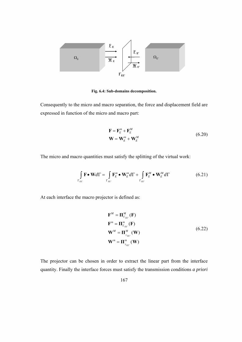
167

ΩEΩE’

ΓEE’

F E

F E’

W E

W E’

ΩEΩE’

ΓEE’

F E

F E’

W E

W E’

Fig. 6.4: Sub-domains decomposition.

Consequently to the micro and macro separation, the force and displacement field are

expressed in function of the micro and macro part:

m ME E

m ME E

= +

= +

F F F

W W W (6.20)

The micro and macro quantities must satisfy the splitting of the virtual work:

' ' 'EE EE EE

m m M ME E E Ed d d

Γ Γ Γ

• Γ = • Γ + • Γ∫ ∫ ∫F W F W F W (6.21)

At each interface the macro projector is defined as:

'

'

'

'

( )

( )

( )

( )

EE

EE

EE

EE

M M

m m

M M

m m

Γ

Γ

Γ

Γ

=

=

=

=

F Π F

F Π F

W Π W

W Π W

(6.22)

The projector can be chosen in order to extract the linear part from the interface

quantity. Finally the interface forces must satisfy the transmission conditions a priori

168

(in the case of perfect interfaces, macro-displacement can also be made continuous a

priori).

To solve this problem the LATIN method [92] is applied. The LATIN method is an

iterative resolution technique which takes into account the whole time interval

studied. At each iteration, an homogenized macroproblem, defined over the whole

time-space domain, is solved as well as a set of independent microproblems which

are linear evolution problems defined within each substructure or at boundaries

between the substructures. The LATIN method, illustrated in Fig. 6.5, is based on the

idea of dealing the difficulties separately, splitting the equations in two subsets:

'

Static and kinematic admissibility:( , ), ( , )

Macro equilibrium:0

E E E E Ed

M ME E

A

⎧⎪ ∀ ∈⎪⎨⎪⎪ + =⎩

σ F ε W M Ω

F F

(6.23)

Dissipation law of each substructure

The behavior and equilibrium at interfaces⎧

Γ ⎨⎩

(6.24)

Ad is the space of the global linear equations defined, while G is the space of the local

nonlinear equations.

169

E+

sn

E-

sn+1sref.

sn+1/2

E+

sn

E-

sn+1sref.

sn+1/2

Fig. 6.5: LATIN scheme for one iteration.

The solution of the problem is obtained by an iterative scheme. Each iteration

consists of a local step and a linear step: the method permits to find a solution that

verifies alternatively the equations of the first and second set of equations and at last

it converges towards the solution sref.

6.5. Numerical results

In this simple example a clamped beam, schematically illustrated in Fig. 6.6,

subjected to an horizontal pressure was analyzed. Two tests were performed: the first

one with the use of a single material and the second one with two different materials.

The results obtained with the application of FETI method and of the mixed method

were put in comparison.

The beam properties are reported in the following:

Geometrical characteristics:

o Brick: rectangular cross section, b=100 mm and h=100 mm; o Mortar: rectangular cross section, b=4 mm and h=100 mm; o External load: horizontal pressure P=10 MPa.

170

Mechanical properties:

o Brick: E=1785 MPa; n=0.2; o Mortar: E=1785 MPa; n=0.2.

LP

LP

Fig. 6.6: Beam scheme.

The mesh is reported in Fig. 6.7, while in Fig. 6.8 it is remarked the single sub-domain considered.

Fig. 6.7: Beam mesh.

Fig. 6.8: Beam sub-domain.

Two analysis are effected, with the application of the FETI method and the mixed method. In the following figures are reported the displacement and stress fields; the results are the same for the two methods.

171

Fig. 6.9: Case 1, displacement field for FETI.

Fig. 6.10: Case 1, displacement field for the mixed method.

Fig. 6.11: Case 1, stress field for FETI.

Fig. 6.12: Case 1, stress field for the mixed method.

172

The same clamped beam, schematically illustrated in Fig. 6.6, subjected to the same

horizontal pressure was re-analyzed considering different mechanical properties for

the two materials:

Geometrical characteristics:

o Brick: rectangular cross section with b=100 mm; h=100 mm; o Mortar: rectangular cross section with b=4 mm; h=100 mm; o External load: horizontal pressure P=10 MPa.

Mechanical properties:

o Brick: E=1785 MPa; n=0.2; o Mortar: E=113 MPa; n=0.2.

In this case it is evident that the second material is effectively more deformable and

at interface some local effects are visible, as illustrated in the following.

Fig. 6.13: Case 2, displacement field for FETI.

Fig. 6.14: Case 2, stress field for FETI.

173

Also in this case the analysis was conduced by the mixed method and the results are

perfectly the same, as illustrated in Fig. 6.15 and Fig. 6.16.

Fig. 6.15: Case 2, displacement field for the mixed method.

Fig. 6.16: Case 2, stress field for the mixed method.

Moreover these results were put in comparison with the classical theoretical results

and with the results obtained by FEAP using the implemented three nodes finite

element; in particular in Tab. 6.1 and in Tab. 6.2 are reported the axial displacement

values for the first and second case, respectively.

FETI MIXED FEAP THEORIC

w [mm] ≈5.58 ≈5.88 ≈5.83 ≈5.83

Tab. 6.1: Case 1 results.

FETI MIXED FEAP THEORIC

w [mm] ≈11.16 ≈9.07 ≈12.53 ≈12.53

Tab. 6.2: Case 2 results.

All the results are in good accordance.

174

The conclusion after the study of this simple example is the possibility of applying

these methods to analyze reinforced masonry arches, reducing the solution of a great

problem into the solution of a set of simplest problems. In fact, once defined the

mesh, with a manual or automatic mesh generator, the subdivision in subdomains is

immediate and the study of the single sub-structure could become simple enough, in

terms both of numerical procedures and computational resource requirement. It must

be emphasized that the domain decomposition methods are adapted to parallel

processing, consisting of independent tasks having their own data that can be

allocated to the various processors of the system. The DDM offer a framework where

different design services can provide the models of their own parts of a structure,

each assessed independently, and they can evaluate the behavior of the complete

structure just setting specific behavior at interfaces. From an implementation point of

view, often programming DDM can be added to existing solvers as an upper level of

current code.

175

CONCLUSIONS

The research activity presented in this thesis work has been focused on the

experimental and numerical analysis of masonry arches strengthened with fiber

reinforced plastic (FRP) materials.

The experimental program regarded different tests performed on both masonry

constituents (bricks and mortar) and structures (unstrengthened and FRP-

strengthened arches). From the performed tests, important aspects concerning the

effect of the FRP reinforcement on the structural response of masonry arches was

observed. In fact, comparing the behavior of unstrengthened and FRP-strengthened

arches, it was observed that the application of FRP at extrados surface of arches

produces an increase both in terms of load-bearing capacity (strength) and in terms of

ultimate displacement (ductility). These effects are related to the collapse

mechanism. In fact, while in the case of unreinforced arches the collapse is due to the

formation of the classic four hinges, the FRP-strengthening prevents the crack

opening at the extrados, i.e. the presence of hinges at intrados, and leads to a collapse

mechanism characterized by shear and crushing failure of masonry.

On the basis of the experimental observations and in order to understand further

aspects concerning the nonlinear response of FRP-strengthened masonry arches, in

the second part of the thesis numerical analyses have been developed. In particular,

two models have been considered for the masonry material; both the models assume

the masonry material characterized by no-tension behavior and limited compressive

strength. For reduced values of the compressive strain, the first one considers a linear

stress strain relationship, while the second one considers a quadratic relationship. In

order to solve the nonlinear unreinforced and reinforced masonry arch problem, a

stress formulation, based on the complementary energy, and a displacement

formulation, based on the implementation of a three nodes finite element into the

FEAP code, have been developed.

176

Moreover, as the delamination phenomenon between the FRP and the masonry

support can play an important role in terms of FRP-strengthening contribution, an

effective procedure, based on a simplified approach of the multiscale method for the

evaluation of the normal and tangential stresses at the interface has been developed.

Moreover, in the context of the multiscale approaches, the domain decomposition

methods are analyzed.

Numerical applications based on the use of the proposed models have been

developed with reference to the performed experimental tests. The comparison

between the numerical and the experimental results demonstrated the ability of the

proposed models to reproduce the global and local response of unstrengthened and

FRP-strengthened arches. In particular, while in the case of the unstrengthened

arches the two proposed models give the same results, in the case of the FRP-

strengthened arch substantial differences occur between the two considered models.

In fact, in this case the second model gives the best results both in terms of pre and

post-peak behavior.

177

APPENDIX: RELUIS SCHEDE

MODELLO PER LA DESCRIZIONE

SINTETICA DI PROVE SPERIMENTALI

STRUTTURE/ELEMENTI STRUTTURALI

IN MURATURA

SPERIMENTAZIONE DI ARCHI IN

MURATURA CON E SENZA RINFORZO IN

FRP

CANCELLIERE ILARIA, RICAMATO MARIA, SACCO ELIO

178

ISTRUZIONI Il modello è diviso in quattro sezioni:

1) Dati generali della prova sperimentale (G)

2) Descrizione elemento/ struttura testata (D)

3) Proprietà dei materiali (M)

4) Risultati della prova (R)

La compilazione delle prime due sezioni richiede l’inserimento di figure con fotografie e/o disegni

che si ritengono utili alla comprensione del setup di prova.

La sezione materiali è basata su tabelle da compilare con i risultati disponibili per mattoni, malta e

muratura. Cliccando sulle relative tabelle si apre una finestra di Excel in cui sono disponibili tutti i

comandi dell’applicazione. In alternativa è possibile copiare nello stesso spazio una qualsiasi tabella

dai contenuti analoghi a quella già predisposta.

La sezione finale non ha un formato prestabilito e la sua compilazione è lasciata agli autori della

prova.

E’ possibile inserire in ciascuna sezione tutte le pagine necessarie alla descrizione della prova e dei

risultati. La numerazione delle pagine ha il formato:

codice sezione/N. totale di pagine della sezione – numero progressivo di pagina

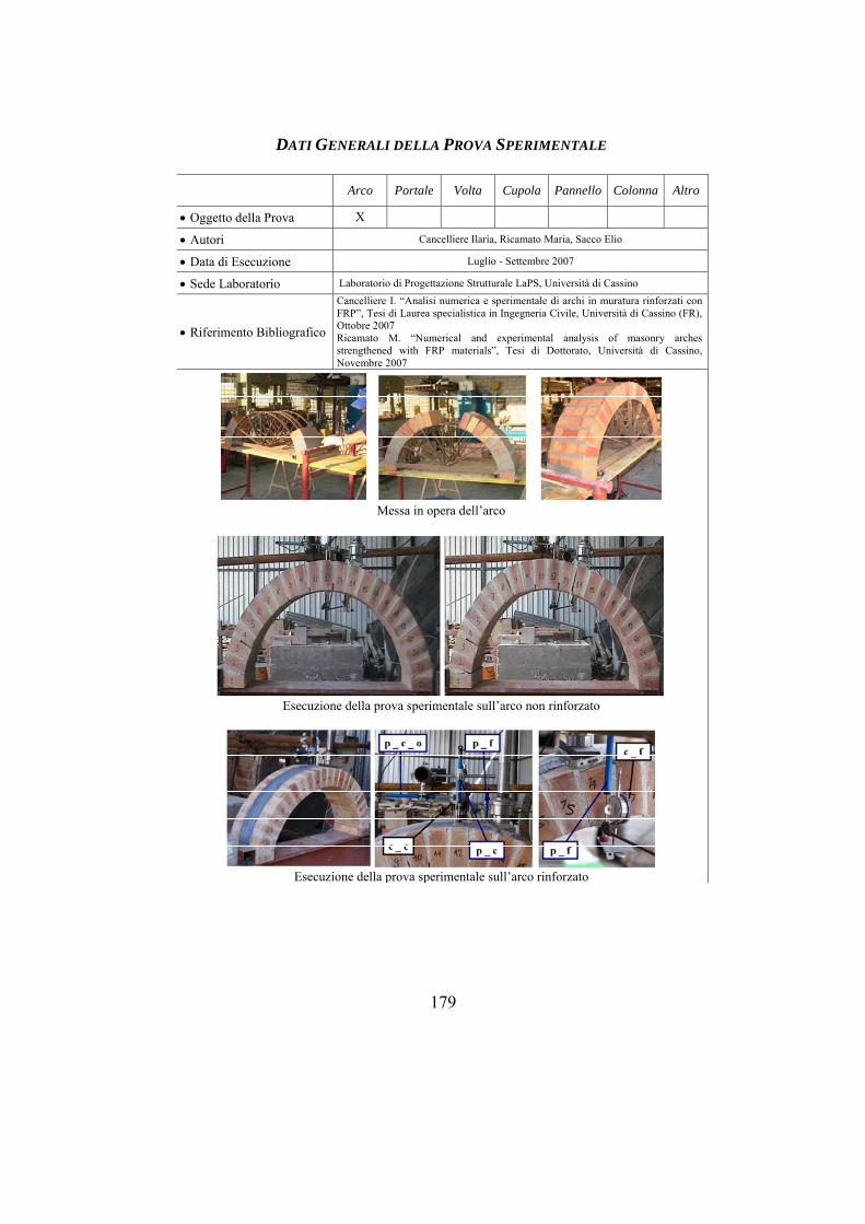
179

DATI GENERALI DELLA PROVA SPERIMENTALE

Arco Portale Volta Cupola Pannello Colonna Altro

• Oggetto della Prova X

• Autori Cancelliere Ilaria, Ricamato Maria, Sacco Elio

• Data di Esecuzione Luglio - Settembre 2007

• Sede Laboratorio Laboratorio di Progettazione Strutturale LaPS, Università di Cassino

• Riferimento Bibliografico

Cancelliere I. “Analisi numerica e sperimentale di archi in muratura rinforzati con FRP”, Tesi di Laurea specialistica in Ingegneria Civile, Università di Cassino (FR), Ottobre 2007 Ricamato M. “Numerical and experimental analysis of masonry arches strengthened with FRP materials”, Tesi di Dottorato, Università di Cassino, Novembre 2007

Messa in opera dell’arco

Esecuzione della prova sperimentale sull’arco non rinforzato

Esecuzione della prova sperimentale sull’arco rinforzato

180

DESCRIZIONE SETUP DI PROVA

Geometria e Vincoli

ReRiRbF i 8 [°] 0.1396 [rad]F f 172 [°] 3.0004 [rad]F c 164 [°] 2.8609 [rad]

576.07 [mm]456.07 [mm]516.07 [mm]

Vincoli L’arco è stato fissato alla base tramite elementi di contrasto per la realizzazione di una condizione di incastro. Note: Il carico è stato applicato mediante un martinetto idraulico disposto in posizione eccentrica. Tra l’estradosso dell’arco e il martinetto è stata posizionata la cella di carico. Sono stati utilizzati tre potenziometri e due comparatori: un potenziometro e un comparatore in direzione verticale in corrispondenza del martinetto; un potenziometro ed un comparatore in direzione verticale in chiave dell’arco; un potenziometro in direzione orizzontale posizionato in chiave.

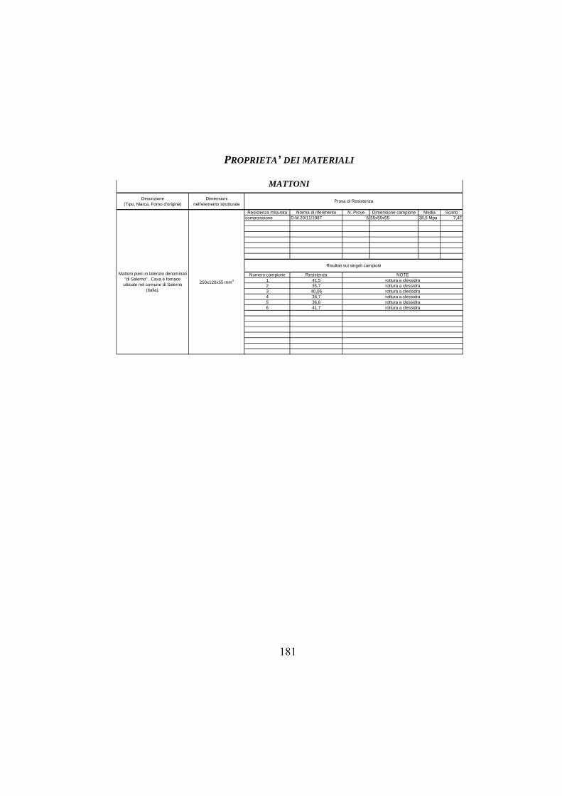
181

PROPRIETA’ DEI MATERIALI

Descrizione(Tipo, Marca, Forno d'origine)

Dimensioninell'elemento strutturale

Resistenza misurata Norma di riferimento N. Prove Dimensione campione Media Scartocompressione D.M.20/11/1987 6 55x55x55 38,5 Mpa 7,47

Numero campione Resistenza1 41,52 35,73 40,064 34,75 36,66 41,7

MATTONI

NOTErottura a clessidra

Prova di Resistenza

Mattoni pieni in laterizio denominati "di Salerno". Cava e fornace

ubicate nel comune di Salerno (Italia).

250x120x55 mm3

rottura a clessidrarottura a clessidrarottura a clessidrarottura a clessidra

Risultati sui singoli campioni

rottura a clessidra

182


DescrizioneSpessore

dei letti di malta nell'elemento strutturale

Resistenza misurata Norma di riferimento N. Prove Dimensione campione Media Scartoflessione UNI-EN 196/1 3 40x40x160 2,53flessione UNI-EN 196/1 3 40x40x160 2,54

compressione D.M.20/11/1987 6 40x40x80 8,75compressione D.M.20/11/1987 6 40x40x80 9,03

Numero campione Resistenza1 2,362 2,623 2,59

1 2,692 2,663 2,27

1 9,1472 9,44753 8,19374 8,48065 9,0086 8,22

1 9,832 9,853 8,3554 8,875 8,536 8,75

MALTA

NOTE

Prova di Resistenza

Malta bastarda: pozzolana, calce aerea, cemento pozzolanico (Duracem 32.5R) ed acqua

il valore medio misurato sulla struttura messa in opera è pari a 15 mm.


183


Resistenza misurata(trazione,

compressione, taglio)

Tipo di prova(compressione diagonale,

compressione, etc..)Norma di riferimento N. Prove Dimensione campione Media Scarto

Numero campione Resistenza

Descrizione della prova(modalità di applicazione del carico, diagrammi carico spostamento, setup di prova, figure del campione, etc..)

MURATURA


NOTE(modalità di rottura, etc..)

Prova di Resistenza

184


FIBRE

Descrizione:

proprietà unità di misura Metodo di prova normativa di riferimento Note

Spessore (lamina) 0.17 mm

larghezza 100 mm

lunghezza 162 mm

Geometria della sezione (barre, cavi)

Area nominale (barre, cavi) mm2

Perimetro nominale (barre, cavi) mm

Colore nero

fibra 1.80 g/cm3 densità

matrice 1.31 g/cm3 ISO 1183-1:2004 (E)

in peso % Contenuto in fibra

in volume % ISO 11667:1997 (E)

Temperatura di transizione vetrosa della resina (Tg) ISO 11357-2:1999(E) (DSC) ISO11359-2:1999(E) (TMA)

Temperatura limite massima di utilizzo °C

Conducibilità elettrica S/m

Modulo di elasticità normale a trazione 230GPa ISO 527-4,5:1997(E)

Resistenza a trazione (valore medio) 3900 MPa ISO 527-4,5:1997(E)

Resistenza a trazione (valore caratteristico) MPa ISO 527-4,5:1997(E)

Deformazione a rottura a trazione 1.5 % ISO 527-4,5:1997(E)

Modulo di elasticità normale a compressione (barre) GPa ISO 14126:1999(E)

Resistenza a compressione (barre) (valore medio) MPa ISO 14126:1999(E)

Resistenza a compressione (barre) (valore caratteristico) MPa ISO 14126:1999(E)

Deformazione a rottura per compressione (barre) % ISO 14126:1999(E)

Resistenza a creep ISO 899-1:2003(E)

Rilassamento (barre, cavi)

Aderenza: tensione tangenziale (barre, cavi) Prova di pull-out

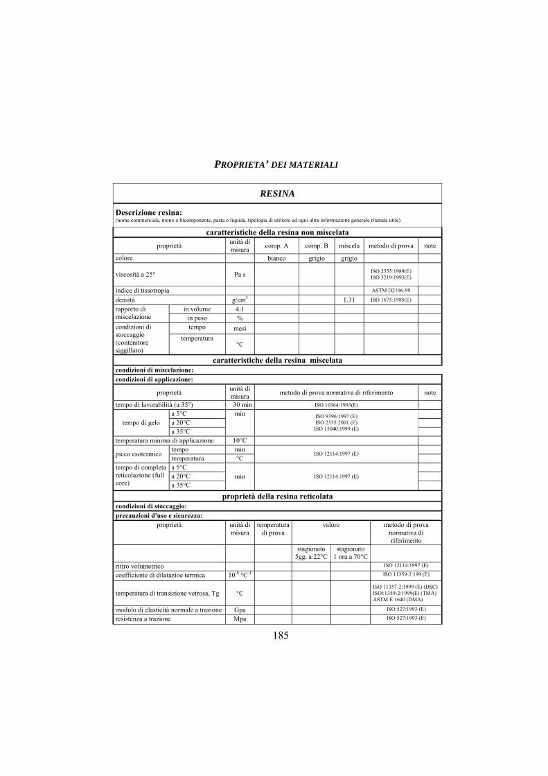
185


RESINA

Descrizione resina: (nome commerciale, mono o bicomponente, pasta o liquida, tipologia di utilizzo ed ogni altra informazione generale ritenuta utile)

caratteristiche della resina non miscelata proprietà unità di

misura comp. A comp. B miscela metodo di prova note

colore bianco grigio grigio

viscosità a 25° Pa s ISO 2555:1989(E) ISO 3219:1993(E)

indice di tissotropia ASTM D2196-99 densità g/cm3 1.31 ISO 1675:1985(E)

in volume 4:1 rapporto di miscelazione in peso %

tempo mesi condizioni di stoccaggio (contenitore siggillato)

temperatura °C

caratteristiche della resina miscelata condizioni di miscelazione: condizioni di applicazione:

proprietà unità di misura metodo di prova normativa di riferimento note

tempo di lavorabilità (a 35°) 30 min ISO 10364:1993(E) a 5°C min a 20°C tempo di gelo a 35°C

ISO 9396:1997 (E) ISO 2535:2001 (E)

ISO 15040:1999 (E) temperatura minima di applicazione 10°C

tempo min picco esotermico temperatura °C

ISO 12114:1997 (E)

a 5°C a 20°C

tempo di completa reticolazione (full core) a 35°C

min ISO 12114:1997 (E)

proprietà della resina reticolata condizioni di stoccaggio: precauzioni d'uso e sicurezza:

proprietà unità di misura

temperatura di prova

valore metodo di prova normativa di riferimento

stagionato 5gg. a 22°C

stagionato 1 ora a 70°C

ritiro volumetrico ISO 12114:1997 (E)

coefficiente di dilatazioe termica 10-6 °C-1 ISO 11359-2:199 (E)

temperatura di transizione vetrosa, Tg °C ISO 11357-2:1999 (E) (DSC) ISO11359-2:1999(E) (TMA) ASTM E 1640 (DMA)

modulo di elasticità normale a trazione Gpa ISO 527:1993 (E)

resistenza a trazione Mpa ISO 527:1993 (E)

186

RISULTATI DELLA PROVA

F(v) in corrispondenza della forza-700.00

-600.00

-500.00

-400.00

-300.00

-200.00

-100.00

0.00

100.00

-7.00-6.50-6.00-5.50-5.00-4.50-4.00-3.50-3.00-2.50-2.00-1.50-1.00-0.500.000.50

v [mm]

F [N

]

Ciclo ICiclo IICiclo III

Cinematismo di collasso e curva forza - spostamento (relativa ai tre cicli di carico e scarico effettuati) per l’arco non rinforzato.

Immagini relative alle fasi di prova dell’arco rinforzato.

F(v) in corrispondenza della forza

-60000

-50000

-40000

-30000

-20000

-10000

0

10000

-23-22-21-20-19-18-17-16-15-14-13-12-11-10-9-8-7-6-5-4-3-2-10123456

v [mm]

F [N

]

Ciclo ICiclo IICiclo III

Curva forza - spostamento (relativa ai tre cicli di carico e scarico effettuati) per l’arco rinforzato. Note

187

NOTATIONS

The following notation were used throughout the text:

Vectors and tensors Quantities

Scalar Vector Second order tensor Third order tensor

a

AA

a

&&

Operators

Inner product Vectorial product Dyadic product Gradient operator

•×⊗Δ

188

Matrices and columns Quantities

1

1

Scalar

Column

Line

Matrix

i

i

ij

aa

a

a a

A

⎧ ⎫⎪ ⎪= ⎨ ⎬⎪ ⎪⎩ ⎭

=

⎡ ⎤= ⎣ ⎦

a

a

A

M

L

Operators

1

Matrix product Transposition Inversion

T

−

ABAA

Any notation which has not been explicitly defined in this section will be explained

at its first point of use.

189

REFERENCES

[1] Drysdale R.G., Hamid A.A., Baker L.R., Masonry Structures, behavior and

design, Prentice Hall, 1994.

[2] Olivito R. S. and Stumpo P., Fracture mechanics in the characterization of

brick masonry structures, Int. J. of Materials and Structures, Vol. 34, 217-

223, 2001.

[3] Hilsdorf H. K., Masonry materials and their physical properties,

Proceedings of the international conference on planning and design of tall

buildings, Vol. III. Bethlehem, Pennsylvania: Lehigh University, 981–1000,

1972.

[4] Carbone I. V., Fiore A. and Pistone G., Le costruzioni in muratura, Hoepli,

Milano, 2001.

[5] Hendry W., Sinha P. B. and Davies S. R., Progetto di strutture in muratura,

Pitagora Editrice, Bologna, 2002.

[6] Lourenço P.B., Experimental and numerical issues in the modelling of the

mechanical behavior of masonry, P. Roca et al. (eds): Structural Analysis of

Historical Constructions II CIMNE, Barcelona, 57-91, 1998.

[7] Van Zijl G., Computational modelling of masonry creep and shrinkage,

PhD thesis, Delft University of Technology, Delft, The Netherlands 2000.

[8] Berto L., Saetta A., Scotta R., Vitaliani R., An orthotropic damage model

for masonry structures, Int. Journal for Numerical Methods in Engineering,

Vol. 55, 127-157, 2002.

[9] Pietruszczak S. and Ushaksaraei R., Description of inelastic behaviour of

structural masonry, Int. J. Solids and Structures; Vol. 40, 4003-4019, 2003.

[10] Lofti H.R. and Shing B.P., Interface model applied to fracture of masonry

structures, Journal of Structural Engineering, ASCE, Vol. 120, 63-80, 1994.

190

[11] Giambanco G. and Di Gati L., A cohesive interface model for the structural

mechanics of block masonry, Mechanics Research Comunications, Vol.

24(5), 503-512, 1997.

[12] Alfano G. and Sacco E., Combining interface damage and friction in a

cohesive-zone model, International Journal for Numerical Methods in

Engineering, Vol. 68(5), 542-582, 2006.

[13] Luciano R, Sacco E. Homogenization technique and damage model for old

masonry material. Int. J. Solids and Structures, Vol. 34 (4), 3191-3208,

1997.

[14] Milani G., Lourenço P.B., Tralli A., Homogenized limit analysis of masonry

walls. Part I: failure surfaces, Comp. Struct., Vol. 84, 166-180, 2006.

[15] Milani G., Lourenço P.B., Tralli A., Homogenised limit analysis of masonry

walls. Part II: structural examples, Comp. Struct., Vol. 84, 181-195, 2006.

[16] Marfia S., Ricamato M., Sacco E., Micro-macro approach for the analysis

of masonry arches reinforced by FRP materials, In progress, 2007.

[17] Lourenço P.B., Continuum model for masonry: parameter estimation and

validation, ASCE Journal of Structural Engineering, Vol. 124 (6), 642-652,

1998.

[18] Marfia S. and Sacco E., Numerical procedure for elasto-plastic no-tension

model, Int. J. for Computational Methods in Eng. Science and Mechanics,

Vol. 6, 187-199, 2005.

[19] Macchi G., General methodology. The combined use of experimental and

numerical techniques inside a single study, P. Roca et al. (eds): Structural

Analysis of Historical Constructions. CIMNE, Barcelona, 10-23, 1997.

[20] Heyman J., The stone skeleton, Cambridge, UK: Cambridge Univ.Press,

1962.

[21] Heyman J., The safety of masonry arches, International Journal of

Mechanical Sciences, 2, 363-385, 1966.

191

[22] Bazant Z.P., Is no-tension design of concrete or rock structures always

safe? Fracture analysis, J Struct. Engrg. ASCE, Vol. 122, 2-10, 1996.

[23] Zienkiewicz O.C., Vallapian S., King I.P., Stress analysis of rock as a

NOTENSION material, Geotechnique, 18, 1968.

[24] Romano G. and Romano M., On the solution of structural problems with

unilateral constitutive relations, Rendiconti di Matematica dell Accademia

dei Lincei, Vol. 68 (8), 104-113, 1979.

[25] Romano G. and Sacco E., No-tension materials: constitutive equations and

structural analysis (in Italian), Istituto di Scienza delle Costruzioni,

University of Naples, Internal Report, 350, 1984.

[26] Del Piero G., Constitutive equations and compatibility of external loads for

linear elastic masonry-like materials, Meccanica, Vol. 24, 150-162, 1989.

[27] Angelillo M., Constitutive relations for no-tension materials, Meccanica,

Vol. 28 (3), 221- 229, 1993.

[28] Angelillo M. and Olivito R.S., Sul comportamento meccanico di pareti in

mattoni, Giornale del Genio Civile, 1-3, 1992.

[29] Giaquinta M. and Giusti E., Researches on the equilibrium of masonry

structures, Arch. Rat. Mech. Analysis, Vol. 88, 359-392, 1988.

[30] Sacco E., Modeling and analysis of structures made of no-tension materials

(in Italian), Rendiconti di Matematica dell Accademia dei Lincei, Vol. 1(9),

235-258, 1990.

[31] Lucchesi M., Padovani C. and Pagni A., A numerical method for solving

equilibrium problems of masonry-like solids, Meccanica, Vol. 29, 175-193,

1994.

[32] Alfano G., Rosati L. and Valoroso N., A numerical strategy for finite

element analysis of no-tension material, Int. J. Num. Meth. Engng., Vol. 48,

317-350, 2000.

192

[33] Grimaldi A., Luciano R., Sacco E., Computational problems for masonry-

like materials, Proceedings of the 11th ABCM Mechanical Engineering

Conference, Sao Paulo (Brazil), December 11-13, 1991.

[34] Luciano R., Sacco E., Stress-penalty method for unilateral contact

problems, Mathematical formulation and computational aspects. European

Journal of Mechanics A/Solids, Vol. 13 (1), 93-111, 1994.

[35] Cuomo M., Ventura G., A complementary energy formulation of no tension

masonry-like solids, Comput. Methods Appl. Mech. Engrg., Vol. 189, 313-

339, 2000.

[36] Lucchesi M., Padovani C. and Zani N., Masonry-like solids with bounded

compressive strength, Int. J. Solids Structures, Vol. 14, 1961-1994, 1996.

[37] Olivito R. S., Statica e stabilità delle costruzioni murarie, Pitagora Editrice

Bologna, 2003.

[38] Triantafillou T. C., Fardis M. N., Strengthening of historic masonry

structures with fiber reinforced plastic composites, in: Leftheris B., Brebbia

C. A. (Eds.), Structural Studies, Repair and Maintenance of Historical

Buildings STREMA 95, Computational Mechanics Publications, 1995.

[39] Croci G., Ayala D., Asdia P. and Palombini F., Analysis on shear walls

reinforced with fibres, IABSE Symp. On Safety and Quality Assurance of

Civil Engineering Structures, Tokyo, Japan, 1987.

[40] Saadatmanesh H., Fiber composites for new and existing structures, ACI

Structural Journal, Vol. 91, 346-354, 1994.

[41] Ehsani M. R., Strengthening of earthquake damaged masonry structures

with composite materials, in Non-metallic (FRP) Reinforcement for

concrete structures. Ed. L. Taerwe, 680-687, 1995.

[42] Luciano R. and Sacco E., Damage of masonry panels reinforced by FRP

sheets, International Journal of Solids and Structures, Vol. 35, 1723-1741,

1998.

193

[43] Marfia S. and Sacco E., Modeling of reinforced masonry elements,

International Journal of Solids and Structures, Vol. 38, 4177-4198, 2001.

[44] Cecchi A., Milani G., Tralli A., In-plane loaded CFRP reinforced masonry

walls: mechanical characteristics by homogenization procedures.

Composites Science and Technology, vol. 64, 2097-2112, 2004.

[45] Schwegler G., Masonry Construction Strengthened with Fibre Composites

in Seismically Endangered Zones, 10th European Conference on Earthquake

Engineering, Rotterdam, 2299-2303, 1995.

[46] Laursen P. T., Seible F., and Hegemier G. A., Innamorato D., Seismic

Retrofit and Repair of masonry Walls with Carbon Overlays, Non-metallic

(FRP) Reinforcement for Concrete structures, Edited by L. Taerwe, RILEM,

616-627, 1995.

[47] Triantafillou T. C., Strengthening of masonry structures using epoxy-bonded

FRP laminates, Journal of Composites for Constructions, ASCE, 2 (1998),

96-103.

[48] Velazquez J. I., Ehsani R., Saadatmanesh H., Out-of-plane cyclic behavior

of URM walls retrofitted with fiber composites, ACI Structural Journal, 377-

387, May-June 2000.

[49] Olivito R. S. and Zuccarello F. A., On the durability of FRP brick masonry

structures subjected to low cycle fatigue, MMSS-FRP, Venezia, 2004.

[50] Croci G. and Viskovic A., L’uso di FRP di fibra aramidica per il rinforzo

della Basilica di San Francesco d’Assisi, Proc. Of Mechanicsw of masonry

structures strengthened with FRP materials, Venezia, Italia, 2000.

[51] Avorio A. and Cecchetti M. V., Applicazione di FRP su archi e volte in

muratura: il caso della Chiesa di San Filippo Neri di Spoleto, Proc. Of

Mechanicsw of masonry structures strengthened with FRP materials,

Venezia, Italia, 2000.

[52] Como M., Ianniruberto U., Imbimbo M., The capacity of masonry arches

strengthened with FRP sheets, Proceeding of the First National Conference

194

“Mechanics of masonry structures strengthened with FRP materials:

modelling, testing, design, control”, Venezia, 2000, (in Italian).

[53] Olivito R. S. and Stumpo P., Analisi numerico-sperimentale di strutture

murarie voltate soggette a carichi mobile, Proc. Nat. Con. XXXI AIAS,

Parma, 2002.

[54] Briccoli Bati S., Rovero L., Consolidation of masonry arches through sheets

of long carbon fibers composites, Proceeding of the First National

Conference “Mechanics of masonry structures strengthened with FRP

materials: modelling, testing, design, control”, Venezia, 2000, (in Italian).

[55] Aiello M. A., Galati N., La Tegola A., Collapse load of masonry arches

strengthened with FRP sheets, Proceeding of the First National Conference

“Mechanics of masonry structures strengthened with FRP materials:

modelling, testing, design, control”, Venezia, 2000, (in Italian).

[56] Chen J. F., Load-bearing capacity of masonry arch bridges strengthened

with fibre reinforced polymer composites, Advances in Structural

Engineering, vol. 5, 37-44(8), 2002.

[57] Luciano R., Marfia S., Sacco E. Reinforcement of masonry arches by FRP

materials. ICCI’02: International Conference on FRP Composites in

Infrastructures, San Francisco, USA, June 10-12, 2002.

[58] Foraboschi P., Strengthening of masonry arches with fiber-reinforced

polymer strips, Journal of Composites for Constructions, ASCE, 191-201,

May-June 2004.

[59] Ianniruberto U., Rinaldi Z., Ultimate behaviour of masonry arches

reinforced with FRP at the intrados: comparison between analytical and

numerical models, Proceedings of the International Seminar on Structural

Analysis of Historical Constructions – Possibilities of Numerical and

Experimental Tecniques, SACH, Padova, 2004.

[60] Olivito R. S., Stumpo P., Tralli A., Stress distribution in FRP reinforced

brick-works, Proc. Int. Conf. CCC2001, Porto, 2001.

195

[61] Olivito R.S., Zuccarello F. A., Milani G., Tralli A., FRP reinforced brick:

delamination tests, Proc. Int. Conf. IPMM, Salerno, 2007.

[62] Riks E., An incremental approach to the solution of snapping and buckling

problems, International Journal of Solids and Structures, vol. 15, 529-551,

1979.

[63] Zienkiewicz O. C. and Taylor R. L., The finite element method, 4th edition,

Mc Graw-Hill, London, 1991.

[64] Hill R., A comparative study of some variational principles in the theory of

plasticity, J. Appl. Mech., 17-64, 1950.

[65] Hill R., Mathematical theory of plasticity, Oxford University Press, Ch. III,

1950.

[66] Prager W. and Hodge P. G., Theory of perfectly plastic solids, Wiley, New-

York, 1951.

[67] Romano G., Scienza delle Costruzioni, Tomo I-II, Hevelius Edizioni, 2001.

[68] Timoshenko S.P., On the correction for shear of the differential equation

for transverse vibration of prismatic bars, Philosophical Magazine, Vol. 41,

744-746, 1921.

[69] Timoshenko S.P., On the transverse vibration of bars of uniform cross-

section, Philosophical Magazine, Vol. 43, 125-131, 1922.

[70] Crisfield M.A., Finite Element and Solution Procedures for Structural

Analysis, Pineridge Press, 1986.

[71] Crisfield M. A., Non-linear Finite Element Analysis of Solids and

Structures, Vol. 1. John Wiley & Sons LTD, England, 1991.

[72] Reddy J.N., An Introduction to the Finite Element Method. McGraw-Hill

International Editions, 1993.

[73] Reddy J.N., On locking-free shear deformable beam finite elements,

Computer Methods in Applied Mechanics and Engineering, vol. 149, pp.

113-132, 1997.

196

[74] Reddy J.N., On the derivation of the superconvergent Timoshenko beam

finite element, Int. J. Comput. Civil and Struct. Engng., vol. 1, No. 2, pp. 71-

84, 2000.

[75] Ortuzar J.M. and Samartin A., Some consistent finite element formulations

of 1-D models: a comparative study, Advances in Engineering Software,

Vol. 29(7-9), 667-678, 1998.

[76] Marfia S., Sacco E., Numerical techniques for the analysis of crack

propagation in cohesive materials, International Journal Numerical Method

in Engineering, vol. 57, 1577-1602, 2003.

[77] Eshelby J.D., The determination of the field of an ellipsoidal inclusion and

related problems, Proceedings of the Royal Society of London, Vol. 241,

376–396, 1957.

[78] Hashin Z., The elastic moduli of heterogeneous materials, ASME Journal

for Applied Mechanics, Vol. 29, 143–150, 1962.

[79] Hill R., A self-consistent mechanics of composites materials, Journal of the

Mechanics and Physics of Solids, Vol. 13, 213–222, 1965.

[80] Mori T. and Tanaka K., Average stress in the matrix and average elastic

energy of materials with misfitting inclusions, Acta Metallurgica, Vol. 21,

571–574,1973.

[81] Christman T., Needleman A. and Suresh S., An experimental and numerical

study of deformation in metal-ceramic composites, Acta Metallurgica,

37(11) : 3029–3050, 1989.

[82] Tvergaard V., Analysis of tensile properties for a whisker-reinforcedmetal-

matrix composite, Acta Metallurgica, Vol. 38(2), 185–194, 1990.

[83] Sluis O., Schreurs P.J.G. and Meijer H.E.H., Effective properties of a

viscoplastic constitutive model obtained by homogenisation, Mechanics of

Materials, Vol. 31, 743–759,1999.

197

[84] Sanchez-Palencia E., Comportement local etmacroscopique d’un type

demilieux physiques hétérogènes, International Journal for Engineering

Science, Vol. 12, 231–251,1974.

[85] Duvaut G., Materiaux élastiques composites à structure périodique

homogénéisation, In Proceedings of the IUTAM Congress, Delft, 1976.

[86] Benssoussan A., Lions J.-L. and Papanicolaou G., Asymptotic Analysis for

Periodic Structures, North-Holland Pub., 1978.

[87] Sanchez-Palencia E., Non homogeneous media and vibration theory, In

Lecture Note in Physics, Vol. 127. Springer Verlag, 1980.

[88] Hughes T. J. R., Multiscale phenomena : Green’s functions, the dirichlet-

toneumann formulation, subgrid scale models, bubbles and the origins of

stabilized methods, Computer Methods in Applied Mechanics and

Engineering, Vol. 127, 387–401, 1995.

[89] Mandel J., Balancing domain decomposition, Communications in Applied

Numerical Methods, Vol. 9, 233–241, 1993.

[90] Farhat C. and Roux F. X., A method of finite element tearing and

interconnecting and its parallel solution algorithm, International Journal for

Numerical Methods in Engineering, Vol. 32, 1205–1227, 1991.

[91] Glowinski R. and Le Tallec P., Augmented lagrangian interpretation of the

nonoverlapping schwartz alternating method, in Third International

Symposium on Domain Decomposition Methods for Partial Differential

Equations, 224–231, Philadelphia, SIAM, 1990.

[92] Ladevèze P., Nonlinear Computational Structural Mechanics - New

Approaches and non-Incremental Methods of Calculation, Springer Verlag,

1999.

[93] Farhat C., Pierson K. and Lesoinne M., A simple an unified framework for

accelerating the convergence of iterative substructuring methods with

lagrange multipliers: Applications to the design of new feti coarse

198

problems, Technical Report CU-CAS-96-26, Center for Aerospaces

Structures, CU, 1996.

[94] Farhat C., Lesoinne M., Le Tallec P., Pierson K. and Rixen D., FETI-DP: A

dual-primal unified FETI method - part i : A faster alternative to the two-

level FETI method, International Journal for Numerical Methods in

Engineering, Vol. 50, 1523–1544, 2001.

[95] Rixen D. and Farhat C., A simple and efficient extension of a class of

substructure based preconditioners to heterogeneous structural mechanics,

International Journal for Numerical Methods in Engineering, Vol. 44, 489–

516, 1999.

[96] Gosselet P. and Ray C., On a selective reuse of krylov subspaces in newton-

krylov approaches for nonlinear elasticity, in Domain decomposition

methods in science and engineering, 419–426, 2002.

[97] Gosselet P., Mèthodes de dècomposition de domaine et mèthodes

d’accèlèration pour les problèmes multichamps en mècanique non-linèaire,

Thèse de doctorat, Universitè Paris 6, 2003.

[98] Ladevèze P. and Dureisseix D., Une nouvelle stratégie de calcul

micro/macro en mécanique des structures, Comptes-Rendus de

l’Acadadémie des Sciences, Vol. 327, 1327–1244, 1999.

[99] Ladevèze P. and Dureisseix D., A micro/macro approach for parallel

computing of heterogeneous structures, International Journal for

Computational Civil and Structural Engineering, Vol. 1, 18–28, 2000.

[100] Ladevèze P., Loiseau O. et Dureisseix D., A micro-macro and parallel

computational strategy for highly heterogeneous structures, International

Journal for Numerical Methods in Engineering, Vol. 52(1-2), 121–138,

2001.

[101] Loiseau O., Une stratégie de calcul multiéchelle pour les structures

hétérogénes, Thése de doctorat, ENS de Cachan, 2001.

199

[102] Allix O., Multiscale strategy for solving industrial problems - Keynote

Lecture, ECCM 2006 - 3d European Conference on Computational

Mechanics, 2006.

[103] Ladevèze P. and Nouy A., A multiscale computational method with time and

space homogeneization, C. R. Mécanique, Vol. 330, 1–7, 2002.

[104] Cresta P., Allix O., Rey C. and Guinard, S., Nonlinear localization

strategies for domain decomposition methods: Application to post-buckling

analyses. Computer Methods in Applied Mechanics & Engineering, Vol

196, 1436-1446, 2007.

Documents

Numerical and experimental analysis of masonry arches ... · Numerical and experimental analysis of masonry arches strengthened with FRP materials Maria Ricamato Cassino, Novembre