NUMERICAL SOLUTION OF

FRACTIONAL DIFFERENTIAL

EQUATIONS AND

APPLICATIONS

INTERNATIONAL WORKSHOP

NSFDE&A'20

SOZOPOL, BULGARIA

S. HARIZANOV, R. LAZAROV, S. MARGENOV (EDS.)

INTERNATIONAL WORKSHOP

NSFDE&A'20

SOZOPOL, BULGARIA

NUMERICAL SOLUTION OF

FRACTIONAL DIFFERENTIAL

EQUATIONS AND

APPLICATIONS

PROCEEDINGS OF SHORT

COMMUNICATIONS

S. HARIZANOV, R. LARAROV, S. MARGENOV (EDS.)

Editors

Stanislav Harizanov

Bulgarian Academy of Sciences

Sofia, Bulgaria

Raytcho Lazarov

Texas A&M University

College Station, Texas, US

Svetozar Margenov

Bulgarian Academy of Sciences

Sofia, Bulgaria

ISBN 978-619-7320-09-1 (eBook)

Institute of Information and Communication Technologies, Bulgarian Academy of Sciences,

Acad. G. Bonchev Str., Bl. 25A, 1113 Sofia, Bulgaria, 2020

PREFACE

The International Workshop on Numerical Solution of Fractional Differential Equa-tions and Applications (NSFDE&A’20) is organized by the Institute of Information andCommunication Technologies, Bulgarian Academy of Sciences, in cooperation with theBulgarian Section of SIAM and the Center of Excellence in Informatics and Informationand Communication Technologies (CoE in Informatics and ICT).

The CoE in Informatics and ICT, Grant No BG05M2OP001-1.001-0003, is financedby the Science and Education for Smart Growth Operational Program (2014-2020) andco-financed by the EU through the European Structural and Investment Funds.

The workshop follows the great success of the Special Session on Fractional DiffusionProblems: Numerical Methods, Algorithms and Applications, organized within the scien-tific program of the 12th International Conference on Large-Scale Scientific Computations(LSSC’19), June 10–14, 2019, Sozopol, Bulgaria. The workshop is aimed to start a newchain of NSFDE&A events to be organized biannually, every even year, complementary tothe well-established LSSC conferences every odd year.

The major specific topics of NSFDE&A’20 include: fractional in space diffusion prob-lems; fractional in time problems; coupled problems; parallel algorithms and high perfor-mance computing tools; applications in science and engineering.

List of keynote speakers and lectures:

1. Raytcho Lazarov (Texas A&M University, College Station, Texas, US)

Solution of Spectral Fractional Elliptic Problems: A Concise Overview of Methods

Based on Rational Approximation

2. Virginia Kiryakova (Institute of Mathematics and Informatics, Bulgarian Academyof Sciences, Sofia, Bulgaria)

Special Functions of Fractional Calculus in Solutions of Fractional Order Equations

and Models

3. HongGuang Sun (State Key Laboratory of Hydrology-Water Resources and HydraulicEngineering, Hohai University, Nanjing, China)

A Survey on Fast Algorithms for Fractional Diffusion Equations and its Applications

The purpose of the workshop is to bring together scientists in the field of numericalmethods working with fractional differential equations models in natural sciences and en-vironmental and industrial applications, as well as developers of algorithms for modernhigh-performance computers. The keynote lectures review some of the most advancedachievements in the field of numerical solution of fractional differential equations and their

i

applications. The workshop talks are presented by scientists from diverse research institu-tions including applied mathematicians, numerical analysts, and computer experts.

Scientists from all over the world (America, Asia, and Europe) contributed to thesuccess of the workshop, representing some of the strongest research groups in the field ofthe event.

This volume contains 23 short communications by authors from 13 countries.The next International Workshop on NSFDE&A will be organized in June 2022.

April 2020 Stanislav HarizanovRaytcho LazarovSvetozar Margenov

ii

Contents

Lidia AcetoFast approximations of fractional powers of operators 1

Anatoly A. AlikhanovA compact difference schemes for the time-fractionaldiffusion equation of variable order 3

A. A. Alikhanov, A. Kh. KhibievA difference analog of a higher approximation order for theCaputo fractional derivative with generalized memory kerneland its application 6

Emanouil Atanassov, Aneta Karaivanova, Sofiya Ivanovska,Mariya DurchovaQuasi-Monte Carlo simulation of fractional Brownianmotion for option pricing using GPUs 7

Hitesh Bansu, Sushil KumarMeshless method for the numerical solution of space andtime fractional wave equation 11

David BolinSpatial modeling of significant wave height using deformedfractional SPDEs 15

Yuri DimitrovApproximations for the second derivative and the Caputofractional derivative 16

S. Harizanov, R. Lazarov, S. Margenov, P. MarinovNumerical stability and accuracy of BURA and URAsolvers for fractional diffusion reaction problems 19

iii

S. Harizanov, R. Lazarov, S. Margenov, P. Marinov,J. PasciakSolution of spectral fractional elliptic problems: A conciseoverview of methods based on rational approximations 23

Clemens HofreitherFast and stable computation of best rationalapproximations with applications to fractional diffusion 27

Ivaylo Katzarov, Nevena Ilieva, Ludmil DrenchevEffective diffusivity of hydrogen in bcc-Fe: Anomalouscharacter due to quantum proton fluctuations? 31

Virginia KiryakovaSpecial functions of fractional calculus in solutions offractional order equations and models 35

N. Kosturski, S. Margenov, Y. VutovBURA methods for large scale fractional diffusionproblems: efficiency of the involved iterative solvers 38

Miroslav KuchtaRobust monolithic solvers for multiphysics systems inbiomechanics 41

Maksim V. KukushkinConvolution operators via the Jacoby series coefficients 45

Yingjie LiangReaction-ultraslow diffusion on comb structures 49

Gabor MarosFractional order elliptic problems with inhomogeneousDirichlet boundary conditions 52

iv

Ivan Matychyn, Viktoriia OnyshchenkoOn computation of the matrix Mittag-Leffler function 56

Neelam SinghaImplementation of fractional optimal control problems inreal-world applications 60

D. Slavchev, S. MargenovNested dissection reordering in a HSS solver for fractionaldiffusion problems 61

HongGuang Sun, Xiaoting LiuA survey on fast algorithms for fractional diffusionequations and its applications 64

Petr N. VabishchevichApproximate representation of the solutions of fractionalelliptical BVP through the solution of parabolic IVP 67

Zhi ZhouSubdiffusion with a time-dependent coefficient: analysisand numerical approximation 70

v

Fast approximations of fractional powers of operators

Lidia AcetoUniversity of Pisa, Italy

Let L be a self-adjoint positive operator with spectrum σ(L) ⊆ [1,+∞), acting ona Hilbert space H endowed with norm ‖·‖

Hand operator norm ‖·‖

H→H. Furthermore,

suppose that L has a compact inverse so that L−α, α ∈ (0, 1), can be written in terms ofthe spectral decomposition of L.

By exploiting the existing representations of the function λ−α in terms of contourintegrals, after suitable changes of variable and quadrature rules one typically finds rationalapproximations of the type

L−α ≈ Rk−1,k(L), Rk−1,k(λ) =pk−1 (λ)

qk (λ), pk−1 ∈ Πk−1, qk ∈ Πk,

where k is an integer closely related to the number of points in the quadrature formula(see, e.g., [1, 2, 4]).

In this talk we focus on a particular integral representation that leads to the use of adouble n-point Gauss-Laguerre rule which implicitly defines a (2n−1, 2n)-rational approx-imation of L−α. Actually, since the functions involved are uniformly bounded with respectto λ ∈ [1,+∞), we consider a truncated approach leading to a rational approximationwhose error is well estimated by

∥

∥

∥L−α −R2kn−1,2kn(L)∥

∥

∥

H→H≈ 8 sin(απ) exp(−5α1/2k1/2

n ),

where kn is the number of inversions of the truncated approach. This approach is veryfast and the quality of the above estimate allows us to define a-priori n and kn in order tosatisfy a given tolerance. The numerical experiments we present confirm the effectivenessof the proposed strategy.

It is worth to mention that this problem finds immediate application when solvingdifferential mathematical models involving a fractional term like (−∆)α, where ∆ denotesthe standard Laplacian [3, 5, 6]. Such models are increasingly used because they provide anadequate description of many processes that exhibit an anomalous diffusion (for example,the diffusion of proteins inside the cells or the diffusion through porous media). In this casethe fractional Laplacian is replaced by the product of two appropriate banded matrices.This leads to a semi-linear initial value problem in which all linear algebra tasks involvesparse matrices with a consequent decrease in computational cost.

This is joint work with Paolo Novati (University of Trieste, Italy).

1

References

[1] L. ACETO, P. NOVATI, Efficient implementation of rational approximations to frac-

tional differential operators. J. Sci. Comput., 76 (2018) pp. 651–671.

[2] L. ACETO, P. NOVATI, Rational approximation to fractional powers of self-adjoint

positive operators. Numer. Math., 143 (2019), pp. 1-16.

[3] L. ACETO, P. NOVATI, Rational approximation to the fractional Laplacian operator

in reaction-diffusion problems. SIAM J. Sci. Comput., 39 (2017) A214–A228.

[4] A. BONITO, J.E. PASCIAK, Numerical approximation of fractional powers of elliptic

operators. Math. Comp., 84 (2015), pp. 2083–2110.

[5] S. HARIZANOV, R. LAZAROV, S. MARGENOV, P. MARINOV, J. PASCIAK, Com-

parison analysis of two numerical methods for fractional diffusion problems based on

the best rational approximations of tγ on [0, 1]. In: Apel T., Langer U., Meyer A.,Steinbach O. (eds) Advanced Finite Element Methods with Applications. FEM 2017.Lecture Notes in Computational Science and Engineering, vol 128. Springer, Cham,2019.

[6] P.N. VABISHCHEVICH, Numerical solution of time-dependent problems with frac-

tional power elliptic operator. Comput. Methods Appl. Math., 18 (2018), pp. 111–128.

2

A compact difference schemes for the time-fractional

diffusion equation of variable order

Anatoly A. AlikhanovInstitute of Applied Mathematics and Automation KBSC RAS

Russia

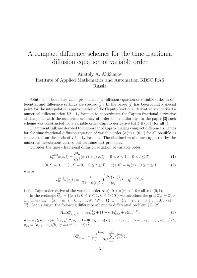
Solutions of boundary value problems for a diffusion equation of variable order in dif-ferential and difference settings are studied [1]. In the paper [2] has been found a specialpoint for the interpolation approximation of the Caputo fractional derivative and derived anumerical differentiation L2− 1σ formula to approximate the Caputo fractional derivativeat this point with the numerical accuracy of order 3− α uniformly. In the paper [3] suchscheme was constructed for a variable order Caputo derivative (α(t) ∈ (0, 1) for all t).

The present talk are devoted to high-order of approximating compact difference schemesfor the time-fractional diffusion equation of variable order (α(x) ∈ (0, 1) for all possible x)constructed on the basis of L2 − 1σ formula. The obtained results are supported by thenumerical calculations carried out for some test problems.

Consider the time - fractional diffusion equation of variable order

∂α(x)0t u(x, t) =

∂2u

∂x2(x, t) + f(x, t), 0 < x < 1, 0 < t ≤ T, (1)

u(0, t) = 0, u(1, t) = 0, 0 ≤ t ≤ T, u(x, 0) = u0(x) 0 ≤ x ≤ 1, (2)

where

∂α(x)0t u(x, t) =

1

Γ(1− α(x))

t∫

0

∂u(x, η)

∂η(t− η)−α(x)dη

is the Caputo derivative of the variable order α(x), 0 < α(x) < 1 for all x ∈ (0, 1).In the rectangle QT = (x, t) : 0 ≤ x ≤ 1, 0 ≤ t ≤ T we introduce the grid ωhτ = ωh×

ωτ , where ωh = xi = ih, i = 0, 1, . . . , N ; hN = 1, ωτ = tj = jτ, j = 0, 1, . . . ,M ; τM =T. Let us assign the following difference scheme to differential problem (1)–(2)

Hh∆αi

0tj+σiyi = σiy

j+1xx,i + (1− σi)y

jxx,i +Hhϕ

j+σi

i , (3)

whereHhvi = vi+h2vxx,i/12, σi = 1− αi

2, αi = α(xi), i = 1, 2, . . . , N−1, vx,i = (vi−vi−1)/h,

vx,i = (vi+1 − vi)/h, vst = (vs+1 − vs)/τ ,

∆αi

0tj+σiv =

τ 1−αi

Γ(1− αi)

j∑

s=0

c(αi)j−sv

st ,

3

τ h e CO in ‖ · ‖C(ωhτ )

1/4 1/16 3.60494e-31/8 1/64 2.42183e-4 3.8961/16 1/256 1.57570e-5 3.9421/32 1/1024 9.82777e-7 4.0031/64 1/4096 6.12760e-8 4.0031/128 1/16384 3.81887e-9 4.0041/256 1/65536 2.38255e-10 4.003

Table 1: Maximum norm error behavior versus grid size reduction when τ = h2

c(αi)0 = a

(αi)0 , for j = 0; and for j ≥ 1,

c(αi)s =

a(αi)0 + b

(αi)1 , s = 0,

a(αi)s + b

(αi)s+1 − b

(αi)s , 1 ≤ s ≤ j − 1,

a(αi)j − b

(αi)j , s = j,

a(αi)0 = σ

1−αi

i , a(αi)l = (l + σi)

1−αi − (l − 1 + σi)1−αi , l ≥ 1;

b(αi)l =

1

2− αi

[

(l + σi)2−αi − (l − 1 + σi)

2−αi]

−1

2

[

(l + σi)1−αi + (l − 1 + σi)

1−αi]

.

If u(x, t) ∈ C6,3x,t and α(x) ∈ C2

x, then the difference scheme has the approximation orderO(τ 2 + h4).

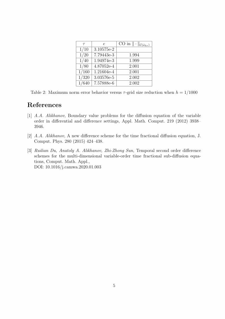
Numerical results. Numerical calculations are performed for a test problem when thefunction u(x, t) = (t4 + 2t3 + 3t2 + 1) sin πx is the exact solution of the problem (1)–(2)with α(x) = 4+sin 5x

6and T = 1.

The errors (e = y − u) and convergence order (CO) in the norm ‖ · ‖C(ωhτ ), where‖y‖C(ωhτ ) = max

(xi,tj)∈ωhτ

|y|, are given in Table 1.

Table 1 shows that as the number of the spatial subintervals and time steps is increasedkeeping h2 = τ , a reduction in the maximum error takes place, as expected and theconvergence order of the approximate scheme is O(h4) = O(τ 2), where the convergence

order is given by the formula: CO= log h1h2

‖e1‖‖e2‖

(ei is the error corresponding to hi).

Table 2 shows that if h = 1/1000, then as the number of time steps of our approximatescheme is increased, a reduction in the maximum error takes place, as expected and theconvergence order of time is O(τ 2), where the convergence order is given by the following

formula: CO= log τ1τ2

‖z1‖‖z2‖

.

Funding: The reported study was funded by RFBR and NSFC according to the researchproject 20-51-53007

4

τ e CO in ‖ · ‖C(ωhτ )

1/10 3.10575e-21/20 7.79443e-3 1.9941/40 1.94974e-3 1.9991/80 4.87052e-4 2.0011/160 1.21604e-4 2.0011/320 3.03576e-5 2.0021/640 7.57888e-6 2.002

Table 2: Maximum norm error behavior versus τ -grid size reduction when h = 1/1000

References

[1] A.A. Alikhanov, Boundary value problems for the diffusion equation of the variableorder in differential and difference settings, Appl. Math. Comput. 219 (2012) 3938–3946.

[2] A.A. Alikhanov, A new difference scheme for the time fractional diffusion equation, J.Comput. Phys. 280 (2015) 424–438.

[3] Ruilian Du, Anatoly A. Alikhanov, Zhi-Zhong Sun, Temporal second order differenceschemes for the multi-dimensional variable-order time fractional sub-diffusion equa-tions, Comput. Math. Appl.,DOI: 10.1016/j.camwa.2020.01.003

5

A difference analog of a higher approximation order for

the Caputo fractional derivative with generalized

memory kernel and its application

A. A. Alikhanov, A. Kh. KhibievInstitute of applied mathematics and automation, Russia

Funding: The reported study was funded by RFBR, project number 19-31-90094

In the present work, a fractional numerical differentiation formula (L2-1σ formula) toapproximate the Caputo fractional derivative of order α(0 < α < 1) with generalizedmemory kernel λ(t) is developed. It is established by means of the quadratic interpolationapproximation using three points (ts−1, u(ts−1), (ts, u(ts)) and (ts+1, u(ts)) for the integrandu(t) on each small interval [ts−1, ts](1 ≤ s ≤ j), while the linear interpolation approximationis applied on the last small interval [tj, tj+σ], where tj+σ is the special super convergencepoints. As a result, the formula can be formally viewed as a modification of the L1 formula,which is obtained in [1]. Both the computational efficiency and numerical accuracy of thenew formula are superior to that of the L1 formula. The coefficients and truncation errorsof this formula are discussed in detail. Test examples show the numerical accuracy of L2-1σformula.

By the new formula, two improved finite difference schemes with high order accuracy intime for solving the time-fractional sub-diffusion equation with generalized memory kernel.Several numerical examples are computed. The comparison with the corresponding resultsof finite difference methods by the L1 formula demonstrates that the L2-1σ formula ismuch more effective and more accurate than the L1 formula when solving time-fractionaldifferential equations with generalized memory kernel numerically.

References

[1] A.A. Alikhanov, A time fractional diffusion equation with generalized memory kernelin differential and difference settings with smooth solutions, Comput. Methods Appl.Math. 2017, 17(4), 647-660

6

Quasi-Monte Carlo simulation of fractional Brownian

motion for option pricing using GPUs

Emanouil Atanassov, Aneta Karaivanova, Sofiya Ivanovska,Mariya Durchova

IICT-BAS, Bulgaria

1 Introduction

The financial options are contracts that give the holder the right to purchase certain secu-rity at a given price or, in more complex cases, provide a payout based on the movementsof the price of the underlying asset. The Monte Carlo method for option pricing is ver-satile and applicable for options with arbitrarily complex payouts. The basic procedurefor obtaining the price of the financial option with payout f(Pt

T0) under the model M is

to simulate multiple paths PtTt=0

of the price of the underlying and evaluate the math-ematical expectation of the discounted payout under the so-called risk-neutral measure,i.e., Price = EQe

−rTf(PtT0). The efficient use of low-discrepancy sequences instead of

pseudorandom numbers gives rise of a QMC method and requires careful study of thesetup of the Monte Carlo method in order achieve improvement of the accuracy. One ofthe basic features of the many statistical models of the price evolution is the use of one ormore Brownian motions in the definition of the model. The fractional Brownian motion(fBM) is an extension that allows for incorporation of long-term memory effects. There aremany relations between fBM and fractional calculus. Although the fractional Laplacianfor α ∈ (] is the generator for the (radially symmetric) 2α-stable Levy process instead, the

fBM observes the following identity for H < H′: BH = (−∆)H′−H

2 BH ′.For more information about these types of relations, see, e.g., [7], while fBM and relatedprocesses are discussed in depth in [3], [4]. A Monte Carlo algorithm for simulating afractional Brownian Motion is well known (see, e.g., [6], also available for Matlab at [2]).We investigated various ways to switch to QMC simulation when using NVIDIA CUDAGPUs for the computations and the respective numerical results.

2 QMC algorithms for simulating fBM and their im-

plementation on NVIDIA GPUs

The basic approach to obtain a QMC algorithm is to use one point of the low-discrepancysequence in order to generate one trajectory of the price of the underlying. The algo-

7

Figure 1: Accuracy of computation of an Asian option

rithm mentioned above requires generation of pseudo-random or quasi-random numbers,multiplication with certain pre-computed constants and performing Fast Fourier Trans-form. NVIDIA CUDA provides fast generation routines with very similar interfaces forgeneration of both pseudo-random numbers and Sobol sequences as well as routines forFFT. We evaluated prices of both European and (arithmetic) Asian options, while thecodes can be used also for exotic options. In the next figure one can see results aboutthe accuracy obtained when computing the same option with 1024 timesteps (construc-tive dimensionality 4096), for number of points ranging from 212 to 222. We comparedthe default pseudorandom generator in CUDA with the default scrambled Sobol sequenceimplemented in CUDA (based on the direction numbers of Joe and Kuo [5]) as well as thedirection numbers provided by Sergei Kucherenko from BRODA ([9]). In all our experi-ments we compute the error as a root-mean-square error (RMSE) using 100 evaluationswith different initial seeds for the scrambling. It is immediately obvious that the QMCalgorithm greatly outperforms in terms of accuracy. The comparison between the differentsets of direction numbers did not yield a definitive conclusion. In the next table one cansee comparison of the computational times, which shows that the advantage of the QMCmethod is not negated by the slightly slower computation. When incorporating additionalscrambling along the ideas of [1], additional 20% are added to the computation time. Theadvantage of GPU vs CPU in such types of computations is dramatic and well established,that is why we do not show such comparisons. Because of the structure of the Monte Carlo

Algorithm / N 12 14 16 18 20 22

CUDA random 0.44 1.45 2.44 4.26 10.17 42.60

CUDA Sobol 0.95 2.41 3.71 4.31 15.07 60.27

Table 1: Computational times for Asian option pricing, when using 2N points

algorithm (pairs of normally distributed random numbers are interpreted as complex num-bers) it is also interesting to replace the basic routine curand normal double / with a fewlines of code using the Box-Mueller transform and curand uniform double . Giray Okten

8

Figure 2: Accuracy of Box-Muller transform vs curand normal double

advocates the use of this transform as superior, see, e.g., [8]. In the next figure one cansee that the accuracy with this transform is substantially better, when using the samedirectional numbers (mean ratio is 1.75 when the number of points grow from 212 to 219).We point out that practitioners in the field usually use only several thousand points, thatis why the results for higher number of points do not have the same weight for practicalapplications.

Conclusions and future work

The numerical and timing results clearly show the advantages of using QMC on GPU forpricing options using fractional Brownian motion in the underlying model. Some advantagein using the Box-Muller transform is observed and is significant enough for practical pur-poses. Additional experiments showed advantage of reordering of the coordinates accordingto their importance can also provide improved accuracy.

Acknowledgments

This work was partially supported by Grant No BG05M2OP001-1.001-0003, financed bythe Science and Education for Smart Growth Operational Program (2014-2020) and co-financed by the EU through the European Structural and Investment Funds.

References

[1] Atanassov E., Ivanovska S. and Karaivanova A., Tuning the Generation of Sobol Se-quence with Owen scrambling, LNCS, vol. 5910, 2010, pp. 459–466.

[2] Botev Z., Fractional Brownian motion generator, MATLAB Central File Exchange.https://www.mathworks.com/matlabcentral/fileexchange/

38935-fractional-brownian-motion-generator Retrieved March 25, 2020.

9

[3] Decreusefond L. and Ustunel A.S., Fractional Brownian Motion: Theory And Applica-tions, ESAIM: PROC, 1998, 75–86.

[4] Decreusefond L. and Ustunel A.S., Stochastic Analysis of the Fractional BrownianMotion, Potential Analysis, 1999, 10:177–214.

[5] Joe S. and Kuo F., Remark on algorithm 659: implementing Sobol’s quasirandomsequence generator. http://portal.acm.org/citation.cfm?id=641879, ACM Trans.on Math. Software, 29(1):49–57, 2003.

[6] Kroese D.P., Botev Z.I., Spatial Process Simulation. In Stochastic Geometry, SpatialStatistics and Random Fields, 2015, pp. 369–404.

[7] Lodhia, Asad; Sheffield, Scott; Sun, Xin; Watson, Samuel S. Fractional Gaussian fields:A survey. Probab. Surveys 13 (2016), 1–56. DOI: 10.1214/14-PS243.

[8] Okten G., Goncu A. , Generating low-discrepancy sequences from the normal distri-bution: Box-Muller or inverse transform?, Mathematical and Computer Modelling, 53(2011), pp. 1268–1281.

[9] Sobol’ I.M., Asotsky D., Kreinin A., Kucherenko S. Construction and Comparison ofHigh-Dimensional Sobol’ Generators, Wilmott, Nov, 2012, 64–79.

10

Meshless method for the numerical solution of space

and time fractional wave equation

Hitesh Bansu Sushil KumarS. V. National Institute of Technology, India

1 Introduction

Fractional order differential equations have attracted many researchers because of theirability to provide extensive and detailed analysis of the model. Fundamental fractionalpartial differential equations are the fractional diffusion equation and the fractional waveequation. Here fractional wave equation is obtained by substituting time and spacederivative with generalised Caputo fractional derivative in the classical wave equation

∂αu(x, t)

∂tα=

∂βu(x, t)

∂xβ+ f(x, t), 1 ≤ α, β ≤ 2, (1)

initial conditions and boundary conditions are

u(x, 0) = p1(x), ut(x, 0) = p2(x)

u(a, t) = q1(t), u(b, t) = q2(t).(2)

Many authors studied the model in equation(1)-(2) with the perspective of numericalsolution. The finite difference method based on the Hermite formula is used by Khaderand Adel [1] for the solution of the wave equation. Sweilam and Nagy [2] implementedthe Crank-Nicholson method to acquire the solution for the fractional wave equation. Inthe present study, we have proposed a novel approach of collocation with Chebyshevpolynomials and radial basis functions for the numerical solution of the fractional waveequation.

2 Preliminaries

In this section, we have discussed an important definition of fractional derivatives, thenotations about Chebyshev polynomials and radial basis functions (RBFs).

Definition 1 Caputo fractional derivative of power function xp, p ≥ 0 is [3]

Dαxp =

Γ(p+1)Γ(p+α−1)

xp−α, for p ≥ ⌈α⌉

0, for p < ⌈α⌉

11

2.1 Radial basis functions

RBFs have become an effective tool for interpolating scattered data in which the univariatefunction u(x) can be approximated as

u (x) =N∑

i=1

λiφi (r),

where λi are coefficients to be determined. N is the number of data points. φ(r) is any RBFand r = ‖x− xi‖ is the Euclidean distance. Most commonly used RBFs are the Gaussian

φ(r) = e−(ǫr)2 , the multiquadric φ(r) = (r2 + ǫ2)β/2, β = −1, 1, 3, .., the polyharmonicsplines φ(r) = rn log r, n = 2, 4, .. and the conical type φ(r) = rn, n = 1, 3, ... In thisstudy we have implemented the conical type RBF with n = 3, called the cubic RBF.

2.2 Chebyshev polynomials

The analytic for of shifted Chebyshev polynomials of degree n is [3, 4]

T ∗n (x) =

n∑

k=0

(−1)n−k22kn (n+ k − 1)!

(2k)! (n− k)!xk.

Using definition (3), fractional derivative of shifted Chebyshev polynomial DαT ∗n (x) is

DαT ∗n (x) =

n∑

k=⌈α⌉

(−1)n−k22kn (n+ k − 1)!

(2k)! (n− k)!

Γ (k + 1)

Γ (k + 1− α)xk−α, n ≥ ⌈α⌉

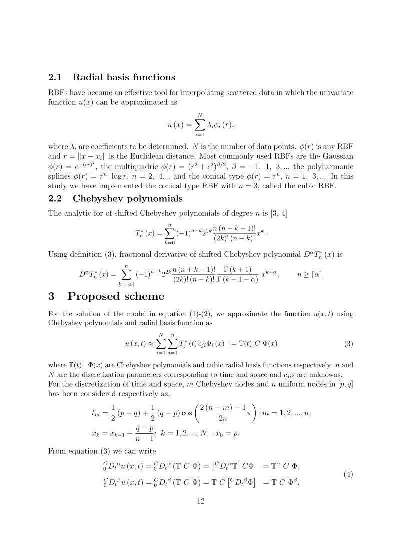
3 Proposed scheme

For the solution of the model in equation (1)-(2), we approximate the function u(x, t) usingChebyshev polynomials and radial basis function as

u (x, t) ≈N∑

i=1

n∑

j=1

T ∗j (t) cjiΦi (x) = T(t) C Φ(x) (3)

where T(t), Φ(x) are Chebyshev polynomials and cubic radial basis functions respectively. n and

N are the discretization parameters corresponding to time and space and cjis are unknowns.

For the discretization of time and space, m Chebyshev nodes and n uniform nodes in [p, q]has been considered respectively as,

tm =1

2(p+ q) +

1

2(q − p) cos

(

2 (n−m)− 1

2nπ

)

;m = 1, 2, ..., n,

xk = xk−1 +q − p

n− 1; k = 1, 2, ..., N, x0 = p.

From equation (3) we can write

C0 Dt

αu (x, t) = C0 Dt

α (T C Φ) =[

CDtαT]

CΦ = Tα C Φ,

C0 Dt

βu (x, t) = C0 Dt

β (T C Φ) = T C[

CDtβΦ

]

= T C Φβ.(4)

12

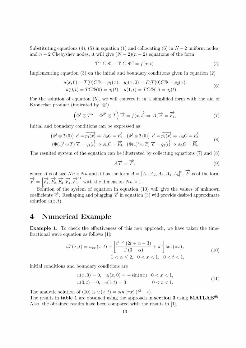
Substituting equations (4), (5) in equation (1) and collocating (6) in N − 2 uniform nodes,and n− 2 Chebyshev nodes, it will give (N − 2)(n− 2) equations of the form

Tα C Φ− T C Φβ = f(x, t). (5)

Implementing equation (3) on the initial and boundary conditions given in equation (2)

u(x, 0) = T (0)CΦ = p1(x), ut(x, 0) = DtT (0)CΦ = p2(x),

u(0, t) = TCΦ(0) = q1(t), u(1, t) = TCΦ(1) = q2(t),(6)

For the solution of equation (5), we will convert it in a simplified form with the aid ofKronecker product (indicated by ‘⊗’)

(

Φt ⊗ T α − Φβt ⊗ T

)

−→c =−−−−→f(x, t) ⇒ A1

−→c =−→F1, (7)

Initial and boundary conditions can be expressed as(

Φt ⊗ T (0))−→c =

−−−→p1(x) ⇒ A2C =

−→F2,

(

Φt ⊗ T (0))−→c =

−−−→p2(x) ⇒ A3C =

−→F3,

(

Φ(1)t ⊗ T)−→c =

−−→q1(t) ⇒ A4C =

−→F4,

(

Φ(1)t ⊗ T)−→c =

−−→q2(t) ⇒ A5C =

−→F5,

(8)

The resulted system of the equation can be illustrated by collecting equations (7) and (8)

A−→c =−→F , (9)

where A is of size Nn×Nn and it has the form A = [A1, A2, A3, A4, A5]t.−→F is of the form

−→F =

[−→F1,

−→F2,

−→F3,

−→F4,

−→F5

]t

with the dimension Nn× 1.

Solution of the system of equation in equation (10) will give the values of unknowncoefficients −→c . Reshaping and plugging −→c in equation (3) will provide desired approximatesolution u(x, t).

4 Numerical Example

Example 1. To check the effectiveness of this new approach, we have taken the time-fractional wave equation as follows [1]:

uαt (x, t) = uxx (x, t) +

[

t1−α (2t+ α− 3)

Γ (3− α)+ π2

]

sin (πx) ,

1 < α ≤ 2, 0 < x < 1, 0 < t < 1,

(10)

initial conditions and boundary conditions are

u(x, 0) = 0, ut(x, 0) = − sin(πx) 0 < x < 1,

u(0, t) = 0, u(1, t) = 0 0 < t < 1.(11)

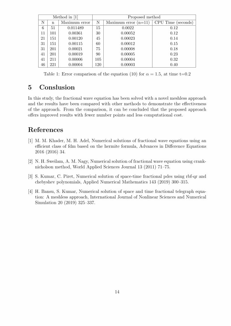
The analytic solution of (10) is u (x, t) = sin (πx) (t2 − t).The results in table 1 are obtained using the approach in section 3 using MATLAB R©.Also, the obtained results have been compared with the results in [1].

13

Method in [1] Proposed method

N n Maximum error N Maximum error (n=11) CPU Time (seconds)

6 51 0.011489 15 0.0022 0.1211 101 0.00361 30 0.00052 0.1221 151 0.00120 45 0.00023 0.1431 151 0.00115 60 0.00012 0.1531 201 0.00021 75 0.00008 0.1841 201 0.00019 90 0.00005 0.2341 211 0.00006 105 0.00004 0.3246 221 0.00004 120 0.00003 0.40

Table 1: Error comparison of the equation (10) for α = 1.5, at time t=0.2

5 Conslusion

In this study, the fractional wave equation has been solved with a novel meshless approachand the results have been compared with other methods to demonstrate the effectivenessof the approach. From the comparison, it can be concluded that the proposed approachoffers improved results with fewer number points and less computational cost.

References

[1] M. M. Khader, M. H. Adel, Numerical solutions of fractional wave equations using anefficient class of fdm based on the hermite formula, Advances in Difference Equations2016 (2016) 34.

[2] N. H. Sweilam, A. M. Nagy, Numerical solution of fractional wave equation using crank-nicholson method, World Applied Sciences Journal 13 (2011) 71–75.

[3] S. Kumar, C. Piret, Numerical solution of space-time fractional pdes using rbf-qr andchebyshev polynomials, Applied Numerical Mathematics 143 (2019) 300–315.

[4] H. Bansu, S. Kumar, Numerical solution of space and time fractional telegraph equa-tion: A meshless approach, International Journal of Nonlinear Sciences and NumericalSimulation 20 (2019) 325–337.

14

Spatial modeling of significant wave height using

deformed fractional SPDEs

David Bolin

Computer, Electrical and Mathematical Science

and Engineering Division,

King Abdullah University of Science and Technology,

Saudi Arabia

A non-stationary Gaussian random field model is developed based on a combination of

the SPDE approach and the classical deformation method. With the deformation method,

a stationary field is defined on a domain which is deformed so that the field is non-stationary

on the new domain. We show that if the stationary field is a Matern field defined as a

solution to a fractional SPDE, the resulting non-stationary model can be represented as the

solution to another fractional SPDE on the deformed domain. By defining the model in this

way, the computational advantages of the rational SPDE approach can be combined with

the deformation methods more intuitive parameterization of non-stationarity. In particular

it allows for essentially independent control over the non-stationary practical correlation

range on one hand and the variance on the other hand. This has not been possible with

previously proposed non-stationary SPDE models.

Numerical methods for the model are based on rational approximations of the fractional

operator in the SPDE, for which explicit convergence rates are available. The model is

tested on spatial data of significant wave height, a characteristic of ocean surface conditions

which is important when estimating the wear and risks associated with a planned journey

of a ship. The model is fitted to data from the north Atlantic and is used to compute

wave height exceedance probabilities and the distribution of accumulated fatigue damage

for ships traveling a popular shipping route. The model results agree well with the data,

indicating that the model could be used for route optimization in naval logistics.

15

Approximations for the second derivative and the

Caputo fractional derivative

Yuri DimitrovDepartment of Mathematics and Physics, University of Forestry,

BulgariaInstitute of Mathematics and Informatics,

Bulgarian Academy of Sciences,Department of Information Modelling

The aim of the report is to propose a method for construction of approximations of theCaputo derivative whose weights have properties similar to the properties of the weights ofthe L1 approximation. The L1 approximation of the Caputo derivative has an order 2−α

and a second order asymptotic formula

1

Γ(2− α)hα

n−1∑

k=0

σ(α)k yn−k = y(α)n +

ζ(α− 1)

Γ(2− α)y′′nh

2−α +O(

h2)

, (1)

σ(α)0

= 1, σ(α)k = (k − 1)1−α − 2k1−α + (k + 1)1−α, σ(α)

n = (n− 1)1−α − n1−α,

where y(α)(x) is the Caputo derivative of order α and h = (x−x0)/n, where x0 is the lowerlimit of fractional differentiation. The weights of the L1 approximation have properties

σ(α)0

> 0, σ(α)1

< σ(α)2

< · · · < σ(α)n−1

< 0. (2)

In [1] we construct approximations of order 2− α of the Caputo derivative whose weightshave properties (2) and we give a proof for the convergence of the numerical solutionsof fractional differential equations which use the approximations. In [2] we construct

approximations of the first derivative which have generating functions A − Aet−1

A and1

Bln(B + 1− Bt). Now we apply the method form [2] for construction of approximations

of the second derivative. Let G1(x) = 2A2e−1/A(

ex/A − e1/A

A(x+ A− 1)

)

. The generating

function G1(x) and the function H1(x) = G1(e−x) have Mclaurin series expansions

G1(x) = 2A− 2A2 + 2A2e−1/A +(

2Ae−1/A − 2A)

x+∞∑

k=2

2e−1/A

k!Ak−2, (3)

H1(x) = x2 −3A+ 1

3Ax3 +

7A2 + 6A+ 1

12A2x4 +O

(

x5)

. (4)

16

The coefficients of the Mclaurin series of the functions G1(x) and H1(x) are the weights ofan approximation of the second derivative and the coefficients of its asymptotic formula:

1

h2

n∑

k=0

w1,ky(x− kh) = y′′(x)−3A+ 1

3Ay′′′(x)h+

7A2 + 6A+ 1

12A2y(4)(x)h2 +O

(

h3)

, (5)

w1,0 = 2A(1− A+ A)e−1/A, w1,1 = −2A(1− e−1/A), w1,k =2e−1/A

k!(A+ 1)k−2.

The approximation (5) requires that y(0) = y′(0) = 0 and it is extended to the classC2[x0, x] by applying a modification of its weights [2]. Let G2(x) =

2

B2 (B − Bx− ln(B +1−Bx)).

G2(x) =2(B − ln(B + 1))

B2−

2x

B + 1+

∞∑

k=2

2Bk−2xk

k(B + 1)k,

H2(x) = G2(e−x) = x2 −

3 + 2B

3x3 +

6B2 + 12B + 7

12x4 +O

(

x5)

.

The approximation of the second derivative with a generating function G2(x) satisfies

1

h2

n∑

k=0

w2,ky(x− kh) = y′′(x)−3 + 2B

3y′′′(x)h+

6B2 + 12B + 7

12y(4)(x)h2 +O

(

h3)

, (6)

w2,0 =2(B − ln(B + 1))

B2, w2,1 = −

2

B + 1, w2,k =

2Bk−2

k(B + 1)k(k ≥ 2).

By approximating the second derivative in (1) with (5) and (6) we obtain the second orderapproximations of the Caputo derivative (i = 1, 2) :

1

Γ(2− α)hα

n−1∑

k=0

δ(α)i,k yn−k = y(α)n +O

(

h2)

, (7)

δ(α)1,0 = 1− 2A(1− A+ Ae−1/A)ζ(α− 1), δ

(α)1,1 = 2α−1 − 2 + 2A(1− e−1/A)ζ(α− 1),

δ(α)1,k = (k − 1)1−α − 2k1−α + (k + 1)1−α −

2A2ζ(α− 1)

e1/Ak!Ak. (8)

δ(α)2,0 = 1−

2

B2ζ(α− 1)(B − ln(B + 1)), δ

(α)2,1 = 2α−1 − 2 +

2ζ(α− 1)

B + 1,

δ(α)2,k = (k − 1)1−α − 2k1−α + (k + 1)1−α −

2ζ(α− 1)Bk−2

k(B + 1)k. (9)

When A = 0.01, B = 10 and α ∈ [0.0002, 0.96] the weights of approximations (8) and(9) satisfy (2). When α ∈ (0, 0.0002) ∪ (0.96, 1) approximations (8) and (9) satisfy (2) for

17

smaller values of the parameter A and larger values of B. The two-term ordinary fractionaldifferential equation

y(α)(x) + y(x) = F (x) = Γ(3− α)x2 + 2x2−α, y(0) = 0 (10)

has a numerical solution

un =1

δ(α)i,0 + Γ(2− α)hα

(

Γ(2− α)hαFn −n−1∑

k=1

δ(α)i,k un−k

)

, u0 = 0. (NS(*))

hα = 0.25, A = 0.01 α = 0.75, B = 5

Error Order Error Order0.003125 3.4473× 10−6 1.9173 9.7697× 10−8 1.95360.0015625 9.0744× 10−7 1.9256 2.4953× 10−8 1.96910.00078125 2.3742× 10−7 1.9344 6.3209× 10−9 1.9810

Table 1: Error and order of numerical solutions NS1(8) and NS1(9) of equation (10).

Acknowledgements

This work is supported by the Bulgarian National Science Fund under Project KP-06-M32/2-17.12.2019 ”Advanced Stochastic and Deterministic Approaches for Large-ScaleProblems of Computational Mathematics”

References

[1] Dimitrov, Y., Approximations for the Caputo derivative (I). Journal of FractionalCalculus and Applications 9(1), 35–63 (2018)

[2] Todorov, V., Dimitrov, Y., Dimov, I. Second order shifted approximations for thefirst derivative. HPC 2019, Borovets, Bulgaria, September 2-6, 2019, accepted forpublication in Studies in Computational Intelligence, Springer series

18

Numerical stability and accuracy of BURA and URAsolvers for fractional diffusion reaction problems

S. Harizanov1, R. Lazarov2, S. Margenov1, P. Marinov1

1Institute of Information and Communication Technologies,Bulgarian Academy of Sciences

2Department of Mathematics, Texas A&M University

This article is devoted to theoretical and experimental comparison analysis of UniformRational Approximation (URA) related numerical solvers of the algebraic problem:

(Aα + qI)u = f , q ≥ 0, α ∈ (0, 1), (1)

where A ∈ RN×N , N ∈ N, is an SPD matrix with eigenvalues and eigenvectors (λi,Ψi)Ni=1

and f ∈ RN is a given vector. For the matrix fractional power Aα the spectral definition

Aα = WDαWT , W = [ΨT1 ,Ψ

T2 , ...,Ψ

TN ], D = diag(λ1, . . . , λN),

is used. Such a problem appears for example in finite element or finite difference discretiza-tion of fractional-in-space diffusion-reaction elliptic problems.

To shorten the exposition, we assume that the spectrum of A is in [1,+∞), i.e., 1 ≤λ1 < λ2 < · · · < λN (otherwise, a normalization with respect to λ−11 needs to be performed).Following [2] and denoting by z(t) := tα, we introduce the function

gq(z(t)) = gq(t;α) :=z

1 + qz=

tα

1 + qtα, t ∈ [0, 1]. (2)

Let k be a given positive integer and α be fixed. The (k, k)-best uniform rational approx-imation (BURA) of gq(t;α) for t ∈ [0, 1] will be denoted by rq(t), while the approximationerror function – by εq(t). In other words

rq(t) = argminr∈R(k,k)

‖r(t)− gq(t;α)‖C[0,1], rq(t) = gq(t;α) + εq(t), Eq := ‖εq‖C[0,1].

The class of functions gq possesses a nice property that motivated us to consider the(k, k)-URA elements as alternative approximations of gq(t;α) (see [1, 2]). Namely,

gq2 gq1 = gq1+q2 ⇒ rq1,q2(t) := gq2 rq1 =rq1(t)

1 + q2rq1(t), q = q1 + q2, q1, q2 ≥ 0.

19

Note that rq1,q2 ∈ R(k, k) for every choice of (q1, q2). Analogously, we define the errorfunction εq1,q2 and its maximal absolute value Eq1,q2 . Assuming that [3, Lemma 2.1] holdstrue for every q1 ≥ 0, we can prove the following error estimates:

‖u− rq(A−1)f‖`2 ≤ Eq‖f‖`2 ,

‖u− rq1,q2(A−1)f‖`2 ≤Eq1(

1 + q2rq1(λ−1N )) (

1 + q2gq1(λ−1N ;α)

)‖f‖`2 , (3)

for any choice of α and q = q1 + q2. Both estimates are almost sharp and cannot beimproved in general. Here, we will analyze Eq in more detail.

We have strong numerical evidence that for all choices of (k, α, q), the value (1 + q)Eqmonotonically increases and is uniformly bounded as q increases . Thus limq→+∞(1+q)Eq =CE0, with constant 1 < C ≤ E−10 , independent on q. In practice, we observe C = O(1) formoderate values of k, meaning that

(1 + q)Eq ∼ E0 ∼ 41+α| sin(πα)|e−2π√αk.

For the approximation of E0 we used the result in [4]. For example, when k = 6 and q = 400we have 401E400/E0 = 5.731, 10.807, 14.804 for α = 0.25, 0.5, 0.75, respectively.

Eq. (3) implies that when an a priori estimate of λN is available, it is sometimes betterto use a (q1, q2)-URA solver rather than the (q1 + q2)-BURA solver. Direct computationsshow that this is the case whenever

λαN <√

(1 + q)(1 + q1) + 1 ⇐⇒ q1 >(λαN − 1)2

1 + q− 1. (4)

In particular, we do not need to compute BURA elements for q > λαN − 2.To illustrate the advantages of the different URA solvers, we consider the matrix

A = tridiag(−1, 2,−1)/h2 with h := 1/(N + 1) that corresponds to FDM of the clas-sical homogeneous 1D Laplace problem in [0, 1] on a uniform grid with mesh-size h. Wehave

Ψi = √

2hsin(ikhπ)Nk=1, λi =4

h2sin2

(iπh

2

), i = 1, . . . , N.

In what follows, we have fixed k = 6 and q = 400, while α = 0.25, 0.5, 0.75. The solverswe compare are generated by the pairs (q1, q2) = (400, 0), (0, 400), (200, 200), (100, 300)and will be referred as BURA, 0-URA, 1-URA, and 2-URA, respectively since

r400,0 = r400, r0,400 = g400 r0, r200,200 = g200 r200, r100,300 = g200 g100 r100.

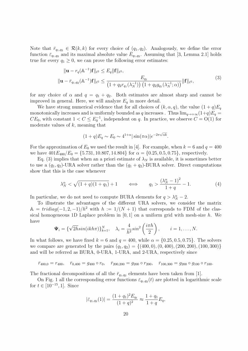
The fractional decompositions of all the rq1,q2 elements have been taken from [1].On Fig. 1 all the corresponding error functions εq1,q2(t) are plotted in logarithmic scale

for t ∈ [10−15, 1]. Since

|εq1,q2(1)| = (1 + q1)2Eq1

(1 + q)2≈ 1 + q1

1 + qEq,

20

α = 0.25 α = 0.50 α = 0.75

10−15

10−10

10−5

100

−1

0

1x 10

−4

BURA

0−URA

1−URA

2−URA

10−15

10−10

10−5

100

−1

−0.5

0

0.5

1x 10

−5

BURA

0−URA

1−URA

2−URA

10−15

10−10

10−5

100

−1

−0.5

0

0.5

1x 10

−6

BURA

0−URA

1−URA

2−URA

Figure 1: Logarithmic plots for the URA errors εq1,q2(t) for t ∈ [10−15, 1], k = 6, q = 400,q1 = 400, 200, 100, 0, and α = 0.25, 0.5, 0.75.

the smaller the q1 the smaller the error function is in vicinity of 1, thus in the right endof the plots interval 0-URA behaves better than 2-URA, which is better than 1-URA, andall are better than BURA. The behavior at the other end of the interval is completely theopposite. For α = 0.5, 0.75 the BURA error function oscillations become smaller thanall the URA-related ones for t < 10−5, respectively t < 10−4, meaning that even on verycoarse meshes (e.g., h ≈ 2 · 10−2) the BURA solver will outperform all the others. Indeed,since λN ≈ 4/h2 we have λαN − 2 ≈ 2h−1 − 2 = 2N , when α = 0.5. Hence, according tothe error analysis above for h = 2 · 10−2 the BURA solver is more accurate than the URAones for q up to approximately 798.

The most interesting case is α = 0.25, where in the same time the BURA advantage isless obvious and the computational efforts for deriving the BURA element are more sub-stantial, due to numerical instability and the necessity to use double-quadruple (or evenhigher for k > 6) precision in the Remez algorithm. Here, we have λαN−2 ≈

√2(N + 1)−2,

so in general no higher q1 than 43, 140, and 446 are needed for optimal accuracy of theURA solvers, when h = 10−3, h = 10−4 and h = 10−5, respectively. This is experimentallyconfirmed in Table 1. For h = 10−3, the BURA solver gives rise to the largest approxima-tion error and even the 0-URA solver is a better candidate. Here the best performance isachieved by the 2-URA solver. For h = 10−4 the 0-URA solver is the least accurate one,while the 1-URA and the 2-URA solvers are the most accurate ones. Still, due to the fasterdecrease in the oscillation margins of the 2-URA method, it remains the best candidate onsuch a mesh size. For h = 10−5 the 0-URA and the 2-URA methods are not reliable any-more, while the BURA and the 1-URA one give rise to practically the same approximationerrors in their worst-case scenarios. Again, the 1-URA method should be preferred dueto the decrease in its oscillations as t increases. On finer grids, the BURA advantage willbe obvious, as this is the only approximation error independent on h. However, for mostof the practical applications no finer grids than h = 10−5 are used in the uniform setting.This is not the case when adaptive refinements are performed.

21

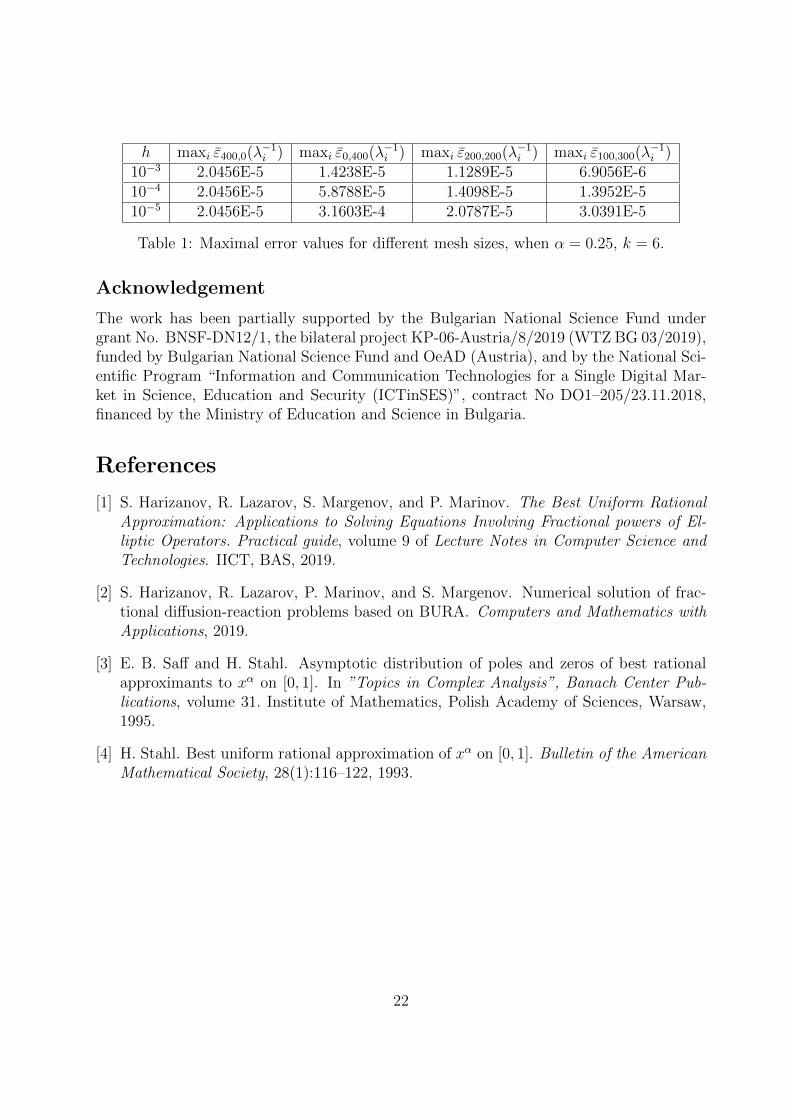
h maxi ε400,0(λ−1i ) maxi ε0,400(λ

−1i ) maxi ε200,200(λ

−1i ) maxi ε100,300(λ

−1i )

10−3 2.0456E-5 1.4238E-5 1.1289E-5 6.9056E-610−4 2.0456E-5 5.8788E-5 1.4098E-5 1.3952E-510−5 2.0456E-5 3.1603E-4 2.0787E-5 3.0391E-5

Table 1: Maximal error values for different mesh sizes, when α = 0.25, k = 6.

Acknowledgement

The work has been partially supported by the Bulgarian National Science Fund undergrant No. BNSF-DN12/1, the bilateral project KP-06-Austria/8/2019 (WTZ BG 03/2019),funded by Bulgarian National Science Fund and OeAD (Austria), and by the National Sci-entific Program “Information and Communication Technologies for a Single Digital Mar-ket in Science, Education and Security (ICTinSES)”, contract No DO1–205/23.11.2018,financed by the Ministry of Education and Science in Bulgaria.

References

[1] S. Harizanov, R. Lazarov, S. Margenov, and P. Marinov. The Best Uniform RationalApproximation: Applications to Solving Equations Involving Fractional powers of El-liptic Operators. Practical guide, volume 9 of Lecture Notes in Computer Science andTechnologies. IICT, BAS, 2019.

[2] S. Harizanov, R. Lazarov, P. Marinov, and S. Margenov. Numerical solution of frac-tional diffusion-reaction problems based on BURA. Computers and Mathematics withApplications, 2019.

[3] E. B. Saff and H. Stahl. Asymptotic distribution of poles and zeros of best rationalapproximants to xα on [0, 1]. In ”Topics in Complex Analysis”, Banach Center Pub-lications, volume 31. Institute of Mathematics, Polish Academy of Sciences, Warsaw,1995.

[4] H. Stahl. Best uniform rational approximation of xα on [0, 1]. Bulletin of the AmericanMathematical Society, 28(1):116–122, 1993.

22

Solution of spectral fractional elliptic problems: Aconcise overview of methods based on rational

approximations

S. Harizanov1,3, R. Lazarov2,3, S. Margenov1, P. Marinov1, J. Pasciak2

1Institute of Information and Communication Technologies,Bulgarian Academy of Sciences

2Department of Mathematics, Texas A&M University,3Institute of Mathematics and Informatics,

Bulgarian Academy of Sciences,

The purpose of the article is to present some new results in approximate solution ofthe problem Aαu = f . Here A is a self-adjoint and coercive elliptic operator defined ona dense subset of L2(Ω), with Ω a bounded Lipschitz domain and 0 < α < 1. We discussthe discretizations Ah of A by finite difference or finite element methods on a mesh withmesh-size h and survey the existence, stability, error, and positivity of the solution of thealgebraic system Aαhuh = fh for uh ∈ RN . The fractional power of the operators A and Ahare defined through their spectra λj, ψj∞j=1 and λj,h, ψj,hNj=1, of A and Ah, respectively,so that

u =∞∑j=1

λ−αj (f, ψj)ψj and uh =N∑j=1

λ−αj,h (fh, ψj,h)ψj,h. (1)

The representation (1) of the approximate solution uh can be used for finding of the so-lution only in the rare case when one knows the discrete spectrum of Ah. However, thisrepresentation could be used to find a suitable approximation using the following reason-ing. Assume that Ah has been properly scaled so that the smallest eigenvalue λ1,h = 1.Let g(t) be some approximation of t−α in L∞([1,∞)). Then

wh =N∑j=1

g(λ−1j,h)(fh, ψj,h)ψj,h := g(A−1h )fh (2)

will be an approximation of uh. Indeed, the L2-norm of the error of this approximation isbounded by

‖uh − wh‖ ≤ maxt∈[1,λN )

|t−α − g(t−1)|‖fh‖ ≤ maxt∈[1,∞)

|t−α − g(t−1)|‖fh‖. (3)

23

To make this a practical algorithm one needs to find the approximation g(t) and to showthat evaluation of g(A−1h )fh is feasible and cheap. An obvious choice for g(t) is the bestuniform polynomial approximation of t−α on [1, λN ]. However, as discussed in [4], this willlead to an inefficient method. Here we shall explore the possibility when g(t) is the bestuniform rational approximation (BURA) of tα on (0, 1], which, as shown in [5], will beequivalent to the best uniform rational approximation of t−α on [1,∞).

Now consider g(t) = rα,k(t), where

rα,k(t) = argmins(t)∈Rk

‖s(t)− tα‖L∞(0,1), (4)

Rk = Pk(z)/Qk(z), with Pk(z), Qk(z) polynomials of degree k and Qk(0) = 1.The problem (4) has been extensively studied in the past, e.g. [8, 9, 12]. Moreover, [9,

Theorem 1], provides an estimate of the error

‖rα,k(t)− tα‖L∞(0,1) ≤ Cαe−2π√kα,

which gives an easy estimate for the the error: ‖uh − wh‖ ≈ Cαe−2π√kα‖fh‖.

Now changing the variable ξ = 1/t in rα,k(t) we get another rational functions definedas

rα,k(ξ) = rα,k(1/t) =tkPk(t

−1)

tkQk(t−1):=

Pk(ξ)

Qk(ξ).

In order to claim that we have an implementable algorithm we need to show that thecomputation of A−αh fh could be done in a stable and efficient way. This is ensured by

the following result [8, 9] regarding the properties of the roots (ζ1, . . . , ζk) of Pk(ξ) and

(d1, . . . , dk) of Qk(ξ): all the roots are real, negative, and interlace so that

0 > dk > ζk > dk−1 > ζk−1 > · · · > d1 > ζ1.

This allows to represent rα,k(ξ) as sum of partial fractions, see e.g. [4, Remark 5.1]

rα,k(t−1) = rα,k(ξ) = c0 +

k∑i=1

ci

ξ − di, with ci > 0, i = 0, 1, . . . , k,

which will lead to the following representation of the approximation wh:

wh =

(c0Ih +

k∑i=1

ci(Ah − diIh)−1)fh, (5)

where Ih is the identity matrix. This solution, called fully discrete, was introduced andstudied in details in [5]. We note that to compute wh we need to solve k systems of the

type (Ah − diIh)vh = fh with symmetric, positive definite and sparse matrices Ah − diIh.For more details on this algorithm and for computing BURA rα,k(t) (its coefficients, rootsand poles) for various values of α and k we refer to [4].

24

We note that due to the properties of the BURA coefficients, computing the approxi-mate solution produces a stable algorithm. Moreover, since the original problem satisfiesthe positivity of the solution (i.e., if f ≥ 0 then u ≥ 0), the solution wh has the sameproperties in the cases when the approximation Ah is done either by finite difference ap-proximation on a rectangular mesh or by lumped mass finite element method (for detailswe refer to [5]).

Further, we discuss some existing methods for solving the problem (1) that are derivedby using equivalent representation of the solution either by Balakrishnan integral repre-sentation formula or by embedding the problem into a relevant PDE problem in a higherdimensional space. These include the methods of Bonito and Pasciak [1, 2], Nochetto,Otarola, and Salgado, [7], (its equivalence to a rational approximation was discovered in[6]), and Vabishchevich, [10] (with improved variants in [3, 11]). We argue that all thesemethods directly or indirectly construct g(t) as some rational approximation of t−α on(λ1,h, λN,h).

Further we argue and computationally show that the solution (5) based on the bestuniform rational approximation (4), introduced and studied in [5], gives a new method,which is as good as the mentioned above methods and in many cases significantly outper-forms them in terms of efficiency, parallelization, and robustness. We also discuss issuesrelated to computing BURA rα,k(t) and implementing the method. Finally, we presentsome numerical experiments on two computational examples involving solution of one-and two-dimensional sub-diffusion problems with smooth and non-smooth data.

Acknowledgement

This research has been partially supported by the Bulgarian National Science Fund undergrant No.BNSF-DN12/1. The work of R. Lazarov was supported in parts by NSF-DMS#1620318 grant. The work of S. Harizanov was supported by the bilateral project KP-06-Austria/8/2019 (WTZ BG 03/2019), funded by Bulgarian National Science Fund andOeAD (Austria).

We acknowledge also the provided access to the e-infrastructure of the Centre for Ad-vanced Computing and Data Processing, with the financial support by the Grant No.BG05M2OP001-1.001-0003, financed by the Science and Education for Smart GrowthOperational Program (2014-2020) and co-financed by the European Union through theEuropean structural and Investment funds.

References

[1] A. Bonito and J. Pasciak. Numerical approximation of fractional powers of ellipticoperators. Mathematics of Computation, 84(295):2083–2110, 2015.

[2] A. Bonito and J. Pasciak. Numerical approximation of fractional powers of regularlyaccretive operators. IMA J Numer Anal, 37(3):1245–1273, 2017.

25

[3] B. Duan, R. D. Lazarov, and J. E. Pasciak. Numerical approximation of fractionalpowers of elliptic operators. IMA Journal of Numerical Analysis, 03 2019. drz013.

[4] S. Harizanov, R. Lazarov, S. Margenov, and P. Marinov. The Best Uniform RationalApproximation: Applications to Solving Equations Involving Fractional powers of El-liptic Operators. Practical guide, volume 9 of Lecture Notes in Computer Science andTechnologies. IICT, BAS, 2019.

[5] S. Harizanov, R. Lazarov, S. Margenov, P. Marinov, and J. Pasciak. Analysis ofnumerical methods for spectral fractional elliptic equations based on the best uniformrational approximation. Journal of Computational Physics, page 109285, 2020.

[6] C. Hofreither. A unified view of some numerical methods for fractional diffusion.Computers and Mathematics with Applications, 2019.

[7] R. H. Nochetto, E. Otarola, and A. J. Salgado. A pde approach to space-time fractionalparabolic problems. SIAM Journal on Numerical Analysis, 54(2):848–873, 2016.

[8] E. B. Saff and H. Stahl. Asymptotic distribution of poles and zeros of best rationalapproximants to xα on [0, 1]. In ”Topics in Complex Analysis”, Banach Center Pub-lications, volume 31. Institute of Mathematics, Polish Academy of Sciences, Warsaw,1995.

[9] H. Stahl. Best uniform rational approximation of xα on [0, 1]. Bulletin of the AmericanMathematical Society, 28(1):116–122, 1993.

[10] P. N. Vabishchevich. Numerically solving an equation for fractional powers of ellipticoperators. Journal of Computational Physics, 282:289–302, 2015.

[11] P. N. Vabishchevich. Approximation of a fractional power of an elliptic operator.arXiv preprint arXiv:1905.10838, 2019.

[12] R. S. Varga and A. J. Carpenter. Some numerical results on best uniform rationalapproximation of xα on [0, 1]. Numerical Algorithms, 2(2):171–185, 1992.

26

Fast and stable computation of best rationalapproximations with applications to fractional diffusion∗

Clemens Hofreither†

Recently there has been significant activity in the development of numerical methodsfor solving elliptic fractional partial differential equations of the type

Lαu = f in Ω,

where α ∈ (0, 1), Ω is a bounded domain, L an elliptic diffusion operator augmented withhomogeneous Dirichlet boundary conditions on ∂Ω, f the right-hand side and u the soughtsolution. After discretization, we can take the point of view that a discrete solution u ∈ Rn

is given by the equation Aαu = f , where A ∈ Rn×n is a symmetric positive definite matrixarising from any number of popular discretization techniques, such as finite differences,finite elements, or isogeometric analysis. An attractive approach to the solution of thisproblem, due to its simplicity and excellent convergence properties, is to compute

u = r(A)f

with a rational function r(x) which is, or is close to, the best uniform rational approx-imation (BURA) to the function x 7→ x−α for x ∈ [λ1, λn], the interval containing thespectrum of A. This approach is particularly appealing since a recent analysis in [3] hasshown that in fact most published methods for solving the fractional diffusion problem canbe interpreted as such rational approximation methods of varying quality, and the use ofBURAs should thus result in a method that is close to optimal. The numerical experimentsin [3] confirm this assumption.

The most recent method in this class is described and analyzed in [2], where the choice

r(x) = λ−α1 r(λ1x−1)

is made with r(x) being the BURA with a chosen degree of the function x 7→ xα in[0, 1]. The method converges exponentially with the degree of r and permits a simple, fullyparallel realization via the partial fraction decomposition which involves solving shiftedproblems with matrices of the form A+ cjI.

∗This work was supported by the bilateral project KP-06-Austria/8/2019 (WTZ BG 03/2019), fundedby Bulgarian National Science Fund and OeAD (Austria).†Johann Radon Insitute for Computational and Applied Mathematics (RICAM), Austria.

27

However, until now a major obstacle to the use of these methods in practice has beenthe computation of the BURAs r(x) ≈ xα. In the recent report [1], the authors provideextensive tables describing these rational approximations for α ∈ 0.25, 0.5, 0.75 and de-grees up to k = 8. These results were produced using a Remez algorithm and in many casesrequired the use of quadruple precision floating point arithmetic and significant computingtime on the order of hours.

Novel ContributionThe aim of this contribution is to describe a novel algorithm, Best Rational Approximationby Successive Interval Length Adjustment (BRASIL), which can compute the (k, k)-BURAof functions of the type x 7→ xα/(1 + qxα), α ∈ (0, 1), q ≥ 0, x ∈ [0, 1], in seconds on astandard workstation, using only standard double precision arithmetic, and with degreesk up to around 80.

The standard approach for computing a (k, k)-BURA, the Remez algorithm, is basedon the idea of finding the 2k+ 2 equioscillation points at which the absolute error assumesits local maxima, shown as stars in Figure 1, right. Between each consecutive pair of suchpoints there lies a point (shown as dots) where the BURA interpolates the exact function.The basic idea of the BRASIL algorithm is to determine the locations (tj)

2kj=0 of these 2k+1

interpolation nodes and compute the BURA by rational interpolation in these nodes.

0.0 0.2 0.4 0.6 0.8 1.0

0.35

0.30

0.25

0.20

0.15

0.10

0.05

0.00

0.0 0.2 0.4 0.6 0.8 1.0

0.006

0.004

0.002

0.000

0.002

0.004

0.006

Figure 1: The function f(x) = x log x, x ∈ [0, 1], together with its (2, 2)-BURA (left) and the resultingerror (right).

A crucial ingredient for computing these rational interpolants in a stable way is theso-called barycentric rational interpolation formula, namely,

r(x) =

∑ki=0

wi

x−xifi∑ki=0

wi

x−xi

,

with nodes xi, values fi, and weights wi, i = 0, . . . , k. This formula describes a rationalfunction r of degree (k, k) with the interpolation property r(xi) = fi, i = 0, . . . , k, as longas wi 6= 0, and in fact it parametrizes all rational functions with this property by varyingthe weights (wi). The barycentric formula is in a sense classical and exhibits superior

28

stability properties, but is still not as widely known in the numerical analysis communityas it deserves to be.

The BRASIL algorithm first determines suitable initial values for the interpolationnodes (tj)

2kj=0 and then in each iteration (1) computes the rational interpolant through these

nodes in barycentric representation, (2) determines the maximum error in each interval(tj, tj+1), (3) shrinks intervals where the error is too large and (4) enlarges intervals wherethe error is too small. These steps are repeated until the maximum errors are equilibratedto a desired tolerance. Some results obtained by this procedure are shown in Table 1.

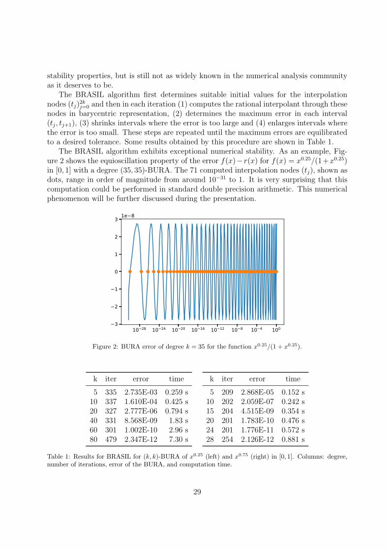
The BRASIL algorithm exhibits exceptional numerical stability. As an example, Fig-ure 2 shows the equioscillation property of the error f(x)− r(x) for f(x) = x0.25/(1+x0.25)in [0, 1] with a degree (35, 35)-BURA. The 71 computed interpolation nodes (tj), shown asdots, range in order of magnitude from around 10−31 to 1. It is very surprising that thiscomputation could be performed in standard double precision arithmetic. This numericalphenomenon will be further discussed during the presentation.

10 28 10 24 10 20 10 16 10 12 10 8 10 4 1003

2

1

0

1

2

3 1e 8

Figure 2: BURA error of degree k = 35 for the function x0.25/(1 + x0.25).

k iter error time

5 335 2.735E-03 0.259 s10 337 1.610E-04 0.425 s20 327 2.777E-06 0.794 s40 331 8.568E-09 1.83 s60 301 1.002E-10 2.96 s80 479 2.347E-12 7.30 s

k iter error time

5 209 2.868E-05 0.152 s10 202 2.059E-07 0.242 s15 204 4.515E-09 0.354 s20 201 1.783E-10 0.476 s24 201 1.776E-11 0.572 s28 254 2.126E-12 0.881 s

Table 1: Results for BRASIL for (k, k)-BURA of x0.25 (left) and x0.75 (right) in [0, 1]. Columns: degree,number of iterations, error of the BURA, and computation time.

29

References

[1] S. Harizanov, R. Lazarov, S. Margenov, and P. Marinov. The best uniform rationalapproximation: Applications to solving equations involving fractional powers of ellipticoperators, 2019. URL https://arxiv.org/abs/1910.13865. arXiv:1910.13865.

[2] S. Harizanov, R. Lazarov, S. Margenov, P. Marinov, and J. Pasciak. Analysis of nu-merical methods for spectral fractional elliptic equations based on the best uniformrational approximation. Journal of Computational Physics, 408:109285, 2020. doi:10.1016/j.jcp.2020.109285.

[3] C. Hofreither. A unified view of some numerical methods for fractional diffusion.Computers & Mathematics with Applications, 2019. doi: 10.1016/j.camwa.2019.07.025.Available online.

30

Effective diffusivity of hydrogen in bcc-Fe: Anomalouscharacter due to quantum proton fluctuations?

Ivaylo Katzarov2, Nevena Ilieva1, Ludmil Drenchev2

1Institute of Information and Communication Technologies,Bulgarian Academy of Sciences

2Institute of Metal Science, Equipment and Technologies,Bulgarian Academy of Sciences

The interactions of hydrogen with crystal defects in α-Fe and their consequences arefundamentally less well understood than diffusion of hydrogen in the perfect crystal lat-tice, despite generally dominating the influence of hydrogen in metals. The existence ofmicrostructural imperfections (vacancies, solute atoms, dislocations, grain boundaries, etc.)introduces trapping sites within the lattice which retard the overall diffusion rate. Intrinsicprocesses in H diffusion are strongly influenced by its quantum mechanical behavior. Atlow temperatures quantum tunneling is expected to be the dominant mechanism, whilethe transition is dominated by classical jumping over the barrier at high temperatures. Inorder to understand the process of H diffusion in Fe, it is essential to study H trappingand migration over the whole range of temperatures covering both the quantum and clas-sical dominated regimes and the crossover between them. Theoretical approaches basedon molecular dynamics (MD) have been used to study H trapping and migration in Fe [1].The state of the art for quantum treatment of the ionic degrees of freedom involves theuse of the ring-polymer MD (RPMD) method [2]. However, including quantum effects iscomputationally demanding compared to a simulation with classical nuclei. The kineticMonte-Carlo (kMC) method has the advantage of being computationally less expensivebecause the interatomic interactions are not computed directly [3]. The fundamental tran-sition rate constants used by kMC can be estimated without knowledge of the dynamicsof the system within the framework of the classical transition state theory (TST). The ap-plication of kMC for the study of H diffusion permits simulations in larger blocks of atomsfor periods of time significantly longer than one can achieve with direct MD simulation,which is essential for studying H migration and trapping in the presence of microstructuralimperfections and consequent extraction of the diffusion coefficients. Unfortunately, clas-sical energy barriers significantly deviate from the experimentally determined activationenergies and kMC simulations using classical transition rates cannot account for quantumcorrections arising from the low mass H atom. A quantum treatment of the hydrogendegrees of freedom is mandatory to capture such effects.

31

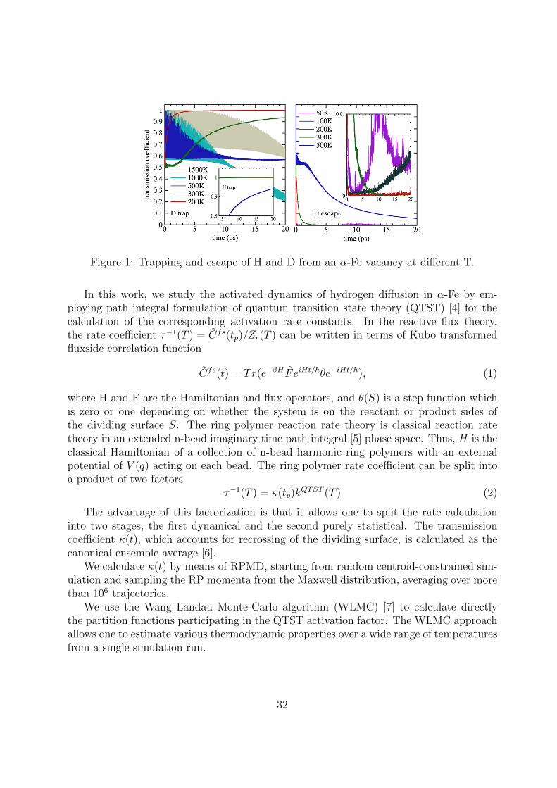
Figure 1: Trapping and escape of H and D from an α-Fe vacancy at different T.

In this work, we study the activated dynamics of hydrogen diffusion in α-Fe by em-ploying path integral formulation of quantum transition state theory (QTST) [4] for thecalculation of the corresponding activation rate constants. In the reactive flux theory,the rate coefficient τ−1(T ) = Cfs(tp)/Zr(T ) can be written in terms of Kubo transformedfluxside correlation function

Cfs(t) = Tr(e−βHF eiHt/hθe−iHt/h), (1)

where H and F are the Hamiltonian and flux operators, and θ(S) is a step function whichis zero or one depending on whether the system is on the reactant or product sides ofthe dividing surface S. The ring polymer reaction rate theory is classical reaction ratetheory in an extended n-bead imaginary time path integral [5] phase space. Thus, H is theclassical Hamiltonian of a collection of n-bead harmonic ring polymers with an externalpotential of V (q) acting on each bead. The ring polymer rate coefficient can be split intoa product of two factors

τ−1(T ) = κ(tp)kQTST (T ) (2)

The advantage of this factorization is that it allows one to split the rate calculationinto two stages, the first dynamical and the second purely statistical. The transmissioncoefficient κ(t), which accounts for recrossing of the dividing surface, is calculated as thecanonical-ensemble average [6].

We calculate κ(t) by means of RPMD, starting from random centroid-constrained sim-ulation and sampling the RP momenta from the Maxwell distribution, averaging over morethan 106 trajectories.

We use the Wang Landau Monte-Carlo algorithm (WLMC) [7] to calculate directlythe partition functions participating in the QTST activation factor. The WLMC approachallows one to estimate various thermodynamic properties over a wide range of temperaturesfrom a single simulation run.

32

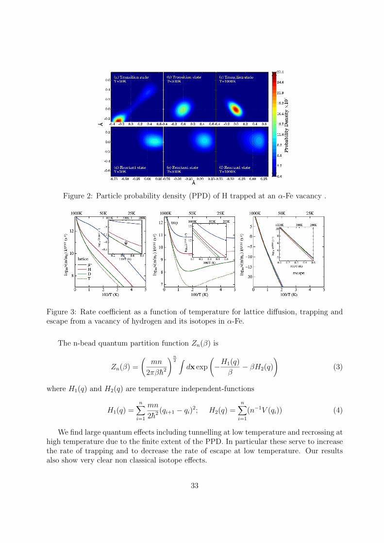
Figure 2: Particle probability density (PPD) of H trapped at an α-Fe vacancy .

Figure 3: Rate coefficient as a function of temperature for lattice diffusion, trapping andescape from a vacancy of hydrogen and its isotopes in α-Fe.

The n-bead quantum partition function Zn(β) is

Zn(β) =

(mn

2πβh2

)n2 ∫

dx exp

(−H1(q)

β− βH2(q)

)(3)

where H1(q) and H2(q) are temperature independent-functions

H1(q) =n∑i=1

mn

2h2 (qi+1 − qi)2; H2(q) =

n∑i=1

(n−1V (qi)) (4)

We find large quantum effects including tunnelling at low temperature and recrossing athigh temperature due to the finite extent of the PPD. In particular these serve to increasethe rate of trapping and to decrease the rate of escape at low temperature. Our resultsalso show very clear non classical isotope effects.

33

Acknowledgements This research was supported in part by the Bulgarian ScienceFund under Grant KP-06-N27/19/17.12.2018, the Bulgarian Ministry of Education andScience (contract D01205/23.11.2018) under the National Research Program “Informationand Communication Technologies for a Single Digital Market in Science, Education andSecurity (ICTinSES)”, approved by DCM # 577/17.08.2018, and the European RegionalDevelopment Fund, within the Operational Programme “Science and Education for SmartGrowth 2014–2020” under the Project CoE “National center of mechatronics and cleantechnologies” BG05M20P001-1.001-0008-C01.

References[1] M. Parrinello and A. Rahman, J. Chem. Phys. 80 (2). 1984, 860-867.

[2] S. Habershon, D.E. Manolopoulos, T.E. Markland, T.F. Miller III, Annu. Rev. Phys.Chem. 64 (2013) 387413.

[3] R. G. Hoagland, A. F. Voter, and S. M. Foiles, Scr. Mat. 39 (1998) 589.

[4] W.H. Miller, S.D. Schwartz, J.W. Tromp, J. Chem. Phys. 79 (10) (1983) 48894898.

[5] Feynman, R.P.; Hibbs, A.R. Quntum Mechanics and Path Integral, McGraw-Hill: NewYork, 1965.

[6] R. Collepardo-Guevara, I.R. Craig, D.E. Manolopoulos, J. Chem. Phys. 128 (14).

[7] F. Wang and D.P. Landau, Phys. Rev. Lett., 86, (2001), 2050.

[8] P.N. Vorontsov-Velyaminov and A.P. Lyubartsev, J. Phys. A: Math. Gen. 36 (2003)685693.

34

Special functions of fractional calculus

in solutions of fractional order equations and models

Virginia KiryakovaInstitute of Mathematics and Informatics,

Bulgarian Academy of Sciences

The developments in theoretical and applied science require knowledge of the propertiesof the “mathematical functions”, from elementary exponential and trigonometric functionsto the variety of Special Functions (SF). These functions appear whenever natural phe-nomena are studied, engineering problems are formulated, and numerical simulations andalgorithms are processed. They also crop up in probability theory and statistics, financialmodels, and economic analysis.

This talk aims to attract attention to classes of SF that were not so popular (or someof them were not introduced) until Fractional Calculus (FC) gained its important role,related to the boom of applications of fractional order models, as better interpretationsand approximations to the real world processes. The so-called Special Functions of Frac-

tional Calculus (SF of FC) are unavoidable tool in exact analytical solutions of fractionalorder (FO) equations, and thus also when their numerical evaluations are to be performed.Under FO equations we mean either integral equations with weak singularities, or dif-ferential equations with ordinary and partial fractional derivatives, or mixtures of thesetypes of equations, among them: ODEs (as fractional relaxation-oscillation equations) andPDEs (as fractional wave-diffusion equations), stochastic fractional differential equations,in control systems of fractional order, quantum mechanics, etc. The SF of FC appear alsoas kernel-functions of the Generalized Fractional Calculus (GFC, [1, 9]) operators; and aspdf-, cdf- or expectations in probability, etc.

The most popular SF of FC are the Mittag-Leffler (ML) functions

Eα(z) =∞∑

k=0

zk

Γ(αk + 1), Eα,β(z) =

∞∑

k=0

zk

Γ(αk + β), α > 0, β ∈ C, (1)

as “fractional index” (α > 0) extensions of the exponential and trigonometric functionslike

exp(z) =∞∑

k=0

zk

Γ(k + 1), cos z =

∞∑

k=0

(−1)kz2k

Γ(2k + 1),

satisfying ODEs of integer order Dny(λz) = λn y(λz), n = 1, 2. In the case of (1), we havefractional order differential equations, for example the simple one, satisfied by the so-calledα-exponential, or Rabotnov function:

35

Dαyα(z) = λ yα(z) with yα(z) = zα−1 Eα,α(λzα), α > 0,

while the ML functions with arbitrary α > 0, β appear in the solutions of various morecomplicated equations of FO.

Although the classical ML functions incorporate a lot of widely used mathematicalfunctions (hyperbolic functions, error functions, incomplete gamma functions, etc), inKiryakova [3, 4, 5], etc., their extension with respect to number of indices has been studiedin details, as including yet another great quantity of SF of FC. These are called multi-index

ML functions :

E(αi),(βi)(z) = E

(m)

(αi),(βi)(z) =

∞∑

k=0

zk

Γ(α1k + β1) . . .Γ(αmk + βm), (2)

with “vector indices” (α1>0, ..., αm>0), (β1, . . . , βm), m = 1, 2, 3, ... . For (2) with m > 1,we have provided a long list of applicable SF of FC, see [3, 4, 5], just to mention: theWright function φ(µ, ν; z) known also as Bessel-Maitland function Jµ

ν (z), Dzrbashjan’s 4-parameters function Φ1/α1,1/α2

(z; β1, β2), the Bessel, Struve, Lommel and Airy functions,the Mainardi function M(z; β) = φ(−β, 1 − β;−z), the hyper-Bessel functions of Delerue

J(m)

ν1,...,νm(z), and so on.

Going further, we note that the multi-index ML functions (2), as well as the 3-parame-ters ML type function (the Prabhakar function) Eγ

α,β(z) and its 3m-parameters extensions(analogous to (2)), are special cases of the Wright generalized hypergeometric functions

(p < q, z ∈ C or p = q + 1, |z| < 1):

pΨq

[

(a1, A1), . . . , (ap, Ap)(b1, B1), . . . , (bq, Bq)

∣

∣

∣

∣

z

]

=∞∑

k=0

Γ(a1 + kA1) . . .Γ(ap + kAp)

Γ(b1 + kB1) . . .Γ(bq + kBq)

zk

k!, (3)

namely,E

(m)

(αi),(βi)(z) = 1Ψm

[

(1, 1)(βi, αi)

m1

∣

∣

∣

∣

z

]

= H1,11,m+1

[

−z

∣

∣

∣

∣

(0, 1)(0, 1), (1− βi, αi)

m1

]

.

For A1 = · · · = Ap = 1, B1 = · · · = Bq = 1, (3) are reduced to the more populargeneralized hypergeometric functions pFq incorporating the “classical” SF, known as “SFof Mathematical Physics”. The functions pΨq and pFq on their side, are representatives ofthe Fox H-functions, resp. of the Meijer G-functions (details, e.g. in Appendix of [1] andrecent handbooks on SF).

Recently, when referring to SF of FC, one has in mind the pΨq- and the FoxH-functions,which for parameters not integer and not rational, are not reduced to the classical SF, thusappearing as tools in solutions of FO differential and integral equations (in general, ofmulti-order (α1, ..., αm)).

Some of our basic results on SF of FC will be briefly discussed, as:– full theory of operators of Generalized FC, introduced in [1] by means of integral ope-

rators with H- and G-functions as kernels, but representable as commutative compositionsof classical operators of FC (Riemann-Liouville, Caputo, Erdelyi-Kober), see also [9];

– all classical SF and all SF of FC can be represented as Generalized FC operators(from [1, 9]) of basic elementary functions (among them exponential, trigonometric, the

36

pdf functions of some probability distributions), see [2, 4]. This can ease the perceptions,applications and numerics for the SF;

– classification and basic properties of SF of FC, see [1, 3, 4, 5], etc.;– evaluation of FC and Generalized FC operators of these SF in the general case of

(3) and of H-functions, thus covering very partial results of hundreds of other recentpublications, see [6, 7, 8], etc.;

– numerous illustrative examples, see within Refs items.For the ML function (1) and some seldom special cases of (2) and (3), numerical

algorithms and plots have been established, by using Maple, Mathematics, etc. But inthe general case of multi-index Mittag-Leffler functions this is still a challenging Open

Problem.

References

[1] Kiryakova, V.: Generalized Fractional Calculus and Applications, Longman-J. Wiley,Harlow-N. York, 1994

[2] Kiryakova, V.: All the special functions are fractional differintegrals of elementaryfunctions, J. Phys. A: Math. & General 30 (14) (1997), 5085–5103

[3] Kiryakova, V.: Multiple (multiindex) Mittag-Leffler functions and relations to general-ized fractional calculus, J. Comput. Appl. Math. 118 (1-2) (2000), 241–259

[4] Kiryakova, V.: The special functions of fractional calculus as generalized fractionalcalculus operators of some basic functions, Computers and Math. with Appl. 59(3)(2010), 1128–1141

[5] Kiryakova, V.: The multi-index Mittag-Leffler functions as an important class of specialfunctions of fractional calculus, Computers and Math. with Appl. 59(5) (2010), 1885-1895

[6] Kiryakova, V.: Fractional calculus operators of special functions? The result is wellpredictable!, Chaos Solutions and Fractals 102 (2017), 2–15

[7] Kiryakova, V.: Commentary: ’A remark on the fractional integral operators and theimage formulas of generalized Lommel-Wright function’, Front. Phys. 7 (2019), # 145,doi:10.3389/fphy.2019.00145

[8] Kiryakova, V.: Fractional calculus of some “new” but not new special functions: K−,multi-index-, and S-analogues, Amer. Inst. of Physics Conf. Proc. 2172 (2019), #050008, doi:10.1063/1.5133527

[9] Kiryakova, V.: Generalized fractional calculus operators with special functions. In:Handbook of Fractional Calculus with Applications, Vol. 1: Basic Theory, Ch. 4, DeGryuter (2019), 87–110

37

BURA methods for large scale fractional diffusion

problems: efficiency of the involved iterative solvers

N. Kosturski, S. Margenov, Y. VutovInstitute of Information and Communication Technologies,

Bulgarian Academy of Sciences

The presented results concern the numerical solution of spectral fractional diffusionproblems in the form Lαu(x) = f(x), where L is a selfadjoint elliptic operator in thebounded domain Ω ⊂ IRd, d ∈ 1, 2, 3, and α ∈ (0, 1]. Two cases are considered: ho-mogeneous pure Dirichlet, and pure Neumann boundary conditions. Let λi, φi(x)

∞i=1 be

the orthonormal spectrum of L. Then, the fractional diffusion operator is defined by thespectral decomposition

Lαv(x) =∞∑

i=i

λαi viφi(x), vi =

∫

Ωφi(x)v(x)dx,

where i = 1, 2 in the first and second case respectively. The finite difference approxi-mation of the problem leads to the system Aαu = f , where A is a sparse, symmetric andpositive (semi)definite matrix, and Aα is defined by a similar spectral decomposition. Inthe case of finite element approximation, A is symmetric with respect to the energy dotproduct associated with the mass matrix.

The fractional diffusion problems are non-local, the matrix Aα is dense, and even notcomputable in the case of large scale problems and general geometry of Ω. Thus, a de-velopment of special numerical methods for efficient solution of such problems is required.Independently, several different methods were proposed, see, e.g., [1, 4]. We study an alter-native approach, based on best uniform rational approximations (BURA) of tα in [0, 1], de-noted by rα,k(x). By assumption, the degree k of the rational function is (relatively) small,see [5, 6] and the references there in. As was shown in [7], the rest known related methodscan be interpreted as some rational approximations. In this sense (and when applicable)the BURA method has certain a priory advantages. In the case of Dirichlet boundary con-ditions, the BURA approximation of u is defined as u ≈ w = λ−α

1 rα,k(λ1A−1)f . Similarly,

in the case of Neumann boundary conditions u ≈ w = λ−α2 rα,k(λ2A

†)f . The method isrobust with respect to the condition number κ(A). In both cases w is expressed in theform w = −b0f −

∑ki=1 bi(A+ ciI)

−1f , thus requiring solving of k auxiliary linear systemswith sparse and symmetric positive definite matrices. The following estimate holds true[6]

||u−w||ℓ2 ≤ Cαλ−α2 e−2π

√kα||f ||ℓ2 ,

38

i.e., the convergence rate with respect to k is exponential.Here, the focus is on the computational efficiency and scalability. Some related results

are available in [2, 3], see also the references there in. The BURA method has almost opti-mal computational complexity, assuming that some optimal solution method is applied tothe involved auxiliary linear algebraic systems. We have used the BoomerAMG implemen-tation of the algebraic multigrid method in the framework of a preconditioned conjugategradient (PCG) iterative solver.

The role of the coefficients bi and ci is analyzed. Larger bi means a stronger impact ofthe solution of the related auxiliary system if, e.g., all bi > 0. The PCG relative stoppingcriteria is properly scaled in order to balance the total error. In addition, larger ci meanssmaller condition number κ(A + ciI), thus decreasing the number of PCG iterations fora fixed stopping criteria. The behaviour of (bi, ci) for α = 0.50 and k = 8 is given in thetable bellow. One can observe that the order of magnitude of the coefficients substantiallyvary. A rich collection of pre-computed data for BURA methods is available in [5].

i 1 2 3 4bi 1.80E − 11 4.73E − 9 3.18E − 7 1.08E − 5ci 7.35E − 8 3.97E − 6 7.56E − 5 8.70E − 4i 5 6 7 8bi 2.41E − 4 3.9E − 3 4.98E − 2 6.14E − 1ci 7.24E − 3 4.78E − 2 2.75E − 1 1.92

The performed numerical results include test problems in 3D domain with complex geome-try. Linear finite elements on unstructured tetrahedral meshes with local mesh refinementare used for discretization of the diffusion operator. The large scale numerical tests arerun on the supercomputer system Avitohol at IICT-BAS. The scalability analysis is madewith respect to the mesh size for α ∈ 0.25, 0.50, 0.75.

Acknowledgments

The partial support through the Grant No BG05M2OP001-1.001-0003, financed by the Sci-ence and Education for Smart Growth Operational Program (2014-2020) and co-financedby the EU through the European Structural and Investment Funds, and through the Bul-garian NSF Grant No DFNI-DN12/1 is highly appreciated.

References

[1] Aceto, L., Novati, P.: Rational approximations to fractional powers of self-adjointpositive operators, Numer Math 143 (2019), 1–16

[2] Bencheva, G., Kosturski, N., Vutov, Y.: Parallel BURA Based Numerical Solution ofFractional Laplacian with Pure Neumann Boundary Conditions, LNCS 11958 (2020),284-291

39

[3] Ciegis, R., Starikovicius, V., Margenov, S., Kriauziene, R.: Scalability analysis of differ-ent parallel solvers for 3D fractional power diffusion problems, Concurrency ComputatPract Exper (2019), https://doi.org/10.1002/cpe.5163

[4] Ciegis, R., Vabishchevich, P.N.: Two-level schemes of Cauchy problem method forsolving fractional powers of elliptic operators, CAMWA (2019), https://doi.org/10.1016/j.camwa.2019.08.012

[5] Harizanov, S., Lazarov, R., Margenov, S., Marinov, P.: The Best Uniform RationalApproximation: Applications to Solving Equations Involving Fractional powers of El-liptic Operators. Practical guide, Lecture Notes in Computer Science and Technologies9 (2019), http://parallel.bas.bg/lcst/2019/09-2019-HLMM.pdf, pp. 85

[6] Harizanov, S., Lazarov, R., Marinov, P., Margenov, S., Pasciak, J.: Analysis of numeri-cal methods for spectral fractional elliptic equations based on the best uniform rationalapproximation, J Comp Phys 408 (2020), https://doi.org/10.1016/j.jcp.2020.109285

[7] Hofreither, C.: A unified view of some numerical methods for fractional diffusion,CAMWA (2019), https://doi.org/10.1016/j.camwa.2019.07.025

40

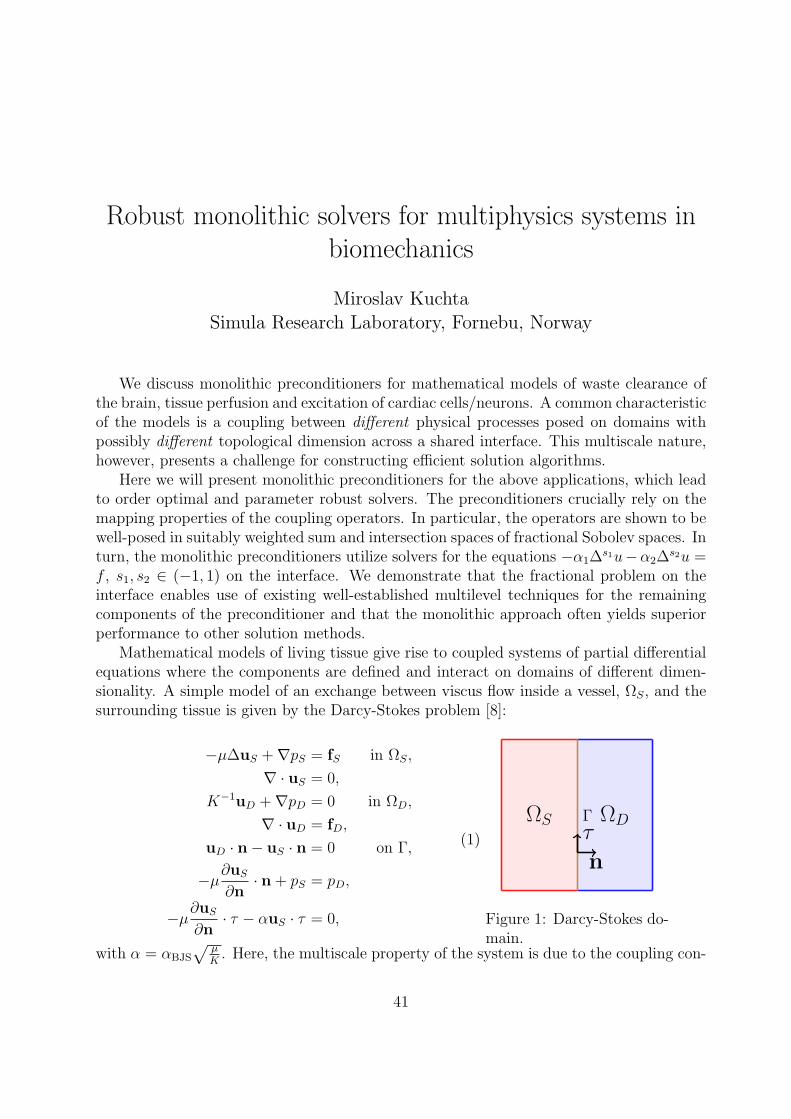
Robust monolithic solvers for multiphysics systems in

biomechanics

Miroslav KuchtaSimula Research Laboratory, Fornebu, Norway

We discuss monolithic preconditioners for mathematical models of waste clearance ofthe brain, tissue perfusion and excitation of cardiac cells/neurons. A common characteristicof the models is a coupling between different physical processes posed on domains withpossibly different topological dimension across a shared interface. This multiscale nature,however, presents a challenge for constructing efficient solution algorithms.

Here we will present monolithic preconditioners for the above applications, which leadto order optimal and parameter robust solvers. The preconditioners crucially rely on themapping properties of the coupling operators. In particular, the operators are shown to bewell-posed in suitably weighted sum and intersection spaces of fractional Sobolev spaces. Inturn, the monolithic preconditioners utilize solvers for the equations −α1∆

s1u−α2∆s2u =

f , s1, s2 ∈ (−1, 1) on the interface. We demonstrate that the fractional problem on theinterface enables use of existing well-established multilevel techniques for the remainingcomponents of the preconditioner and that the monolithic approach often yields superiorperformance to other solution methods.

Mathematical models of living tissue give rise to coupled systems of partial differentialequations where the components are defined and interact on domains of different dimen-sionality. A simple model of an exchange between viscus flow inside a vessel, ΩS, and thesurrounding tissue is given by the Darcy-Stokes problem [8]:

−µ∆uS +∇pS = fS in ΩS,

∇ · uS = 0,

K−1uD +∇pD = 0 in ΩD,

∇ · uD = fD,

uD · n− uS · n = 0 on Γ,

−µ∂uS

∂n· n+ pS = pD,

−µ∂uS

∂n· τ − αuS · τ = 0,

(1)

ΓΩS ΩD

n

τ

Figure 1: Darcy-Stokes do-main.

with α = αBJS

√

µK. Here, the multiscale property of the system is due to the coupling con-

41

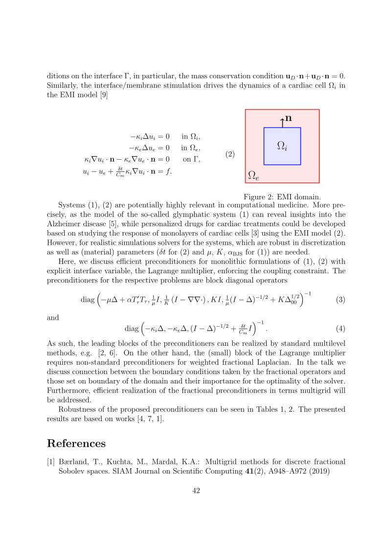
ditions on the interface Γ, in particular, the mass conservation condition uD ·n+uD ·n = 0.Similarly, the interface/membrane stimulation drives the dynamics of a cardiac cell Ωi inthe EMI model [9]

−κi∆ui = 0 in Ωi,

−κe∆ue = 0 in Ωe,

κi∇ui · n− κe∇ue · n = 0 on Γ,

ui − ue +δtCm

κi∇ui · n = f.

(2)Ωi

Ωe

n

Figure 2: EMI domain.Systems (1), (2) are potentially highly relevant in computational medicine. More pre-

cisely, as the model of the so-called glymphatic system (1) can reveal insights into theAlzheimer disease [5], while personalized drugs for cardiac treatments could be developedbased on studying the response of monolayers of cardiac cells [3] using the EMI model (2).However, for realistic simulations solvers for the systems, which are robust in discretizationas well as (material) parameters (δt for (2) and µ, K, αBJS for (1)) are needed.

Here, we discuss efficient preconditioners for monolithic formulations of (1), (2) withexplicit interface variable, the Lagrange multiplier, enforcing the coupling constraint. Thepreconditioners for the respective problems are block diagonal operators

diag(

−µ∆+ αT ′

τTτ ,1

µI, 1

K(I −∇∇·) , KI, 1

µ(I −∆)−1/2 +K∆

1/200

)−1

(3)

and

diag(

−κi∆,−κe∆, (I −∆)−1/2 + δtCm

I

)−1

. (4)

As such, the leading blocks of the preconditioners can be realized by standard multilevelmethods, e.g. [2, 6]. On the other hand, the (small) block of the Lagrange multiplierrequires non-standard preconditioners for weighted fractional Laplacian. In the talk wediscuss connection between the boundary conditions taken by the fractional operators andthose set on boundary of the domain and their importance for the optimality of the solver.Furthermore, efficient realization of the fractional preconditioners in terms multigrid willbe addressed.

Robustness of the proposed preconditioners can be seen in Tables 1, 2. The presentedresults are based on works [4, 7, 1].

References

[1] Bærland, T., Kuchta, M., Mardal, K.A.: Multigrid methods for discrete fractionalSobolev spaces. SIAM Journal on Scientific Computing 41(2), A948–A972 (2019)

42

µK

nh23 24 25 26 27 µ

K

nh23 24 25 26 27

10−6

10−8 62 62 60 59 59

10−2

10−8 52 50 50 50 50

10−6 67 67 66 65 65 10−6 57 56 56 55 55

10−4 73 72 72 71 69 10−4 62 60 60 61 61

10−2 77 76 76 76 75 10−2 64 64 64 65 64

1 75 76 74 76 77 1 58 58 56 56 57

10−4

10−8 57 56 56 55 55

1

10−8 54 52 52 51 53

10−6 62 62 60 59 59 10−6 58 58 57 57 57

10−4 67 67 66 65 65 10−4 60 62 62 61 61

10−2 73 72 70 71 71 10−2 56 56 56 55 55

1 72 72 72 72 73 1 51 50 50 50 50

Table 1: Number of preconditioned MinRes iterations for solving (1) with preconditioner(3). Case αBJS=1 is shown. Uniform 2d mesh consisting of 2nh triangle is considered.

δt

nh Monolithic AMG preconditioner Fractional preconditioner

23 24 25 26 27 28 23 24 25 26 27 28

106 8 8 8 8 8 9 10 10 10 10 10 10

104 8 8 8 8 8 9 15 15 15 15 15 15

102 7 8 8 8 8 9 18 18 18 17 17 17

1 8 8 8 9 9 9 27 27 27 26 26 26

10−2 8 8 9 9 10 10 43 47 46 44 44 43

10−4 28 26 19 14 11 10 49 60 62 60 57 56

10−6 56 81 101 104 87 62 51 60 62 61 59 59

Table 2: Number of Krylov iterations for solving (2). (Left) Symmetric, positive- definiteformulation (without the multiplier) is solved with AMG-preconditioned conjugate gradientmethod. The solver is sensitive to δt. (Right) Saddle point formulation with the Lagrangemultiplier uses (4)-preconditioned MinRes solver. The method is robust in δt.

[2] Falgout, R.D., Yang, U.M.: hypre: A library of high performance preconditioners. In:International Conference on Computational Science. pp. 632–641. Springer (2002)

[3] Grskovic, M., Javaherian, A., Strulovici, B., Daley, G.Q.: Induced pluripotent stemcells—opportunities for disease modelling and drug discovery. Nature reviews Drugdiscovery 10(12), 915–929 (2011)

[4] Holter, K.E., Kuchta, M., Mardal, K.A.: Robust preconditioning of monolithicallycoupled multiphysics problems. arXiv preprint arXiv:2001.05527 (2020)

[5] Jessen, N.A., Munk, A.S.F., Lundgaard, I., Nedergaard, M.: The glymphatic system:a beginner’s guide. Neurochemical research 40(12), 2583–2599 (2015)

[6] Kolev, T.V., Vassilevski, P.S.: Parallel auxiliary space AMG solver for H(div) problems.SIAM Journal on Scientific Computing 34(6), A3079–A3098 (2012)

[7] Kuchta, M., Mardal, K.A.: Iterative solvers for cell-based emi models. In: EMI: cellbased mathematical model of excitable cells, pp. 0–100. Springer (2020)

43

[8] Layton, W.J., Schieweck, F., Yotov, I.: Coupling fluid flow with porous media flow.SIAM Journal on Numerical Analysis 40(6), 2195–2218 (2002)

[9] Tveito, A., Jæger, K.H., Kuchta, M., Mardal, K.A., Rognes, M.E.: A cell-based frame-work for numerical modeling of electrical conduction in cardiac tissue. Frontiers inPhysics 5, 48 (2017)

44

Convolution operators via the Jacoby series coefficients

Maksim V. KukushkinMoscow State University of Civil Engineering, RussiaKabardino-Balkarian Scientific Center, RAS, Russia

In this paper we offer one method of studying some class of convolution operators. Tobe short we do not produce a general scheme of reasonings, but restrict our study for thecase corresponding to the Riemann-Liouville operator. Now we continue studying (see [4])the Abel equation with the right part belonging to a Lebesgue weighted space. We haveimproved the previously known result - the existence and uniqueness theorem formulatedin terms of the Jacoby series coefficients that gives us an opportunity to find and classifya solution due to an asymptotic of some relation containing the Jacoby series coefficientsof the right part. In the beginning, let us remind that the so called mapping theorems forthe Riemann-Liouville operator were firstly studied by H. Hardy and Littlewood, it wasproved that Iαa+ : Lp → Lq, 1 < p < 1/α, q < p/(1 − αp), α ∈ (0, 1). This propositionwas afterwards clarified [1] and nowadays is known as the Hardy-Littlewood theorem withlimit index Iαa+ : Lp → Lq, q = p/(1 − αp). However there was an attempt to extend thistheorem on some class of weighted Lebesgue spaces defined as functional spaces endowedwith the following norm

‖f‖Lp(I, ω) :=

b∫

a

|f(x)|p ω(x)dx

1/p

, ω(x) := (x− a)β(b− x)γ, β, γ ∈ R, I := (a, b).

In this direction the mathematicians such as Rubin B.S. [9, 10, 11], Karapetyants N.K.[2, 3], Vakulov B.G. [15], Samko S.G. [13, 14] (the results of [2, 9, 10] are also presented in[12]) had a great success. There were formulated the analogs of Hardy-Littlewood theoremfor a class of weighted Lebesgue spaces. The main disadvantage of the results presentedin [12] is gaps of the parameters values in the conditions, moreover the notorious problemrelated to p = 1/α was remained completely unsolvable. All these create the prerequisiteto invent another approach for studying the Riemann-Liouville operator action that wassuccessfully applied in the paper [4] and we write out bellow some of its highlights. Weconfirm that the main advantage of the method, used in the paper [4] and based on theresults [7, 8, 5, 6], is still relevant and allows us to obtain some interesting results. Themain challenge of this paper is to improve and clarify the results of the paper [4]. Inparticular we need to find a simple condition, on the right part of the Abel equation,under which Theorem 2 [4] is applicable. For this purpose we have made an attempt to

45

study this problem having used absolute convergence of a series. The main relevance ofthe improvement is based on the fact that the previously used methods were determinedby the relation between order α of the fractional integral and index p of a Lebesgue space(for instance the case p = 1/α is not considered in the monograph [12]). Here we givethe highlights: The relationship between the values of the parameters and order α, byvirtue of which we can provide a description of the solution smoothness, is established;The conditions providing existence and uniqueness of the solution, formulated in terms ofJacoby series coefficients, were obtained. The principal result - the independence betweenone of the parameters and the solution smoothness was proved.

Consider the orthonormal system of the Jacobi polynomials denoted by

p (β,γ)n (x) = δn(β, γ) (x− a)−β(b− x)−γ d

n

dxn

[

(x− a)β+n(b− x)γ+n]

, β, γ > −1, n ∈ N0,

where δn(β, γ) is the normalized multiplier. In the paper [4] we calculate the coefficients

(pm, Iαa+pn)L2(I, ω) = (−1)nAα,β,γ

mn , (pm, Iαb−pn)L2(I, ω) = (−1)mAα,γ,β

mn ,

where the shorthand non standard notation is also used I−αa+ = Dα

a+, α ∈ (0, 1). In thatpaper the first our aim was to reformulate, in terms of the Jacoby series coefficients,the previously known theorems describing the Riemann-Liouville operator action in theweighted Lebesgue spaces. Besides the main results of the paper, we stress that therewas arranged some systematization of the previously known facts of the Riemann-Liouvilleoperator action in the weighted Lebesgue spaces, where the weighted function is representedby some kind of a power function. We managed to fill the gaps of the previously knownresults and formulated this result as a separate Lemma 1 [4]. The following theorem is thevery mapping theorem (see [4]) formulated in terms of the Jacoby series coefficients. Herewe give the modified form corresponding to the right-side case.

Theorem 1. (Theorem 2 in [4]) Suppose

ω(x) := (x− a)β(b− x)γ , β, γ ∈ [−1/2, 1/2], Skf :=

k∑

i=0

p(β,γ)i fi, fi :=

b∫

a

p(β,γ)i (x)f(x)ω(x)dx,

the Pollard condition holds

4max

β + 1

2β + 3,γ + 1

2γ + 3

< p < 4min

β + 1

2β + 1,γ + 1

2γ + 1

,

the right part of the Abel equation Iαb−ϕ = f, α ∈ (0, 1) such that

∥

∥Dαb−Skf

∥

∥

Lp(I, ω)≤ C, k ∈ N0,

∣

∣

∣

∣

∣

∞∑

n=0

fnAα,γ,βmn

∣

∣

∣

∣

∣

≤ Cm−λ, m ∈ N, λ ∈ [0,∞);

46

then there exists a unique solution of the Abel equation in Lp(I, ω), the solution belongs

to Lq(I, ω), where: q = p, if 0 ≤ λ ≤ 1/2 ; q = maxp, t, t < (2s − 1)/(s − λ), if1/2 < λ < s (s = 3/2 + maxβ, γ); q is arbitrary large, if λ ≥ s. Moreover if λ > 1/2,then the solution is represented by the convergent in Lq(I, ω) series

ψ(x) =∞∑

m=0

pm(x)(−1)m∞∑

n=0

fnA−α,γ,βmn . (1)

Theorem 2. Assume that the following series is absolutely convergent

∞∑

n=0

fncn <∞,

where fn are the Jacoby series coefficients of the right part of the Abel equation Iαb−ϕ = f,

cn =δ′nn!Γ(n+ β + 1)Γ(n+ γ + 1)

4n,

the condition γ+1− 2α > 0 holds, then there exists a unique solution of the Abel equation

in accordance with Theorem 1, the solution is represented by series (1), and the value of

the parameter is λ = γ + 3/2− 2α.

References

[1] Hardy G.H., Littlewood J.E. Some properties of fractional integrals I. Mathematische

Zeitschrift, 27, Issue 1 (1928), 565–606.

[2] Karapetyants N.K., Rubin B.S. Operators of fractional integration in spaces with aweight (in Russian). Izv. Akad. Nauk Armyan. SSR, Ser. Mat., 19, No.1 (1984), 31–43.

[3] Karapetyants N.K., Rubin B.S. Radial Riesz potential on the disk and the fractionalintegration operators. Reports of the Academy of Sciences of the USSR, 25, No.2(1982), 522–525.

[4] Kukushkin M.V. Riemann-Liouville operator in weighted Lp spaces via the Jacobyseries expansion. Axioms, 8, No 2:75 (2019), 1–23; https://doi.org/10.3390/

axioms8020075.

[5] Muckenhoupt B. Mean Convergence of Jacobi Series. Proceedings of the American

Mathematical Society, 23, No.2 (Nov., 1969), 306-310.

[6] Newman J., Rudin W. Mean convergence of orthogonal series. Proc. Amer. Math.

Soc., 3, No.2 (1952), 219–222.

[7] Pollard H. The mean convergence of orthogonal series I. Trans. Amer. Math. Soc., 62,No.3 (1947), 387–403.

47

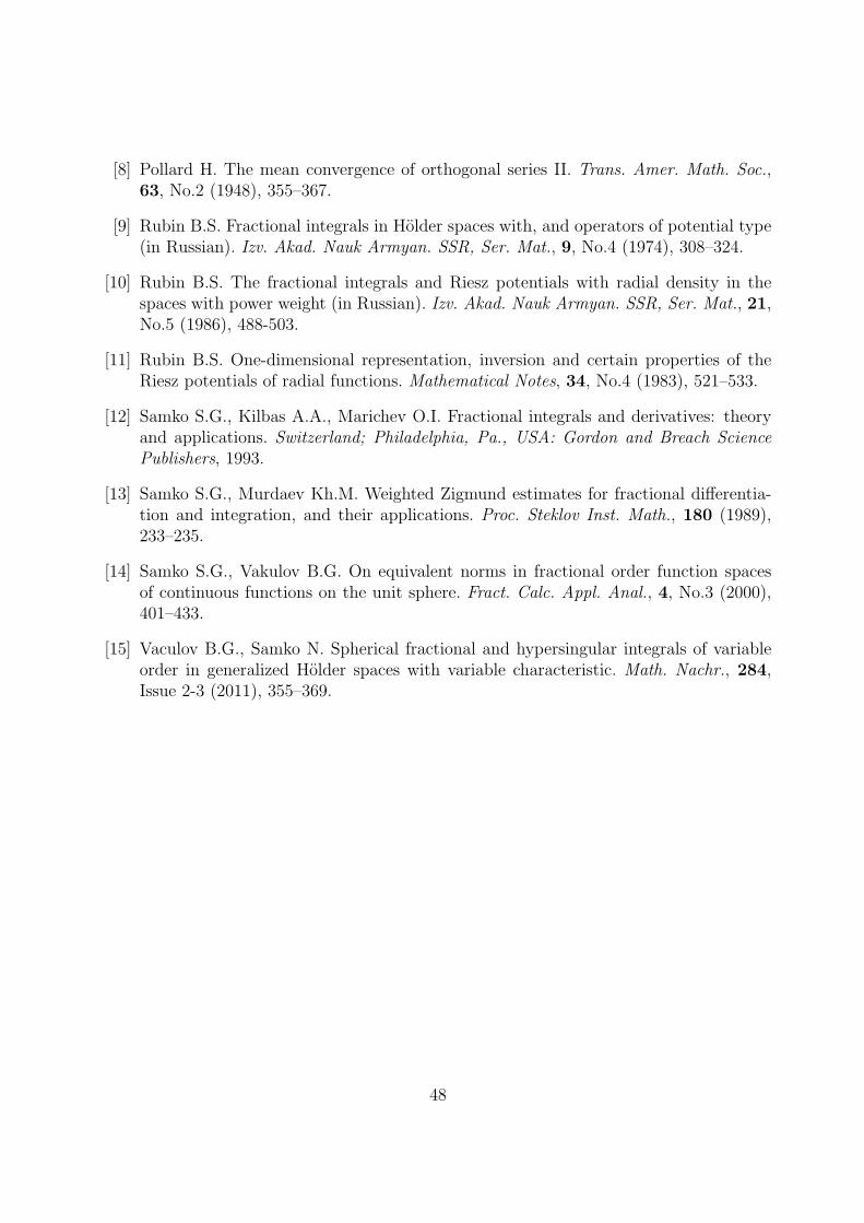
[8] Pollard H. The mean convergence of orthogonal series II. Trans. Amer. Math. Soc.,63, No.2 (1948), 355–367.

[9] Rubin B.S. Fractional integrals in Holder spaces with, and operators of potential type(in Russian). Izv. Akad. Nauk Armyan. SSR, Ser. Mat., 9, No.4 (1974), 308–324.

[10] Rubin B.S. The fractional integrals and Riesz potentials with radial density in thespaces with power weight (in Russian). Izv. Akad. Nauk Armyan. SSR, Ser. Mat., 21,No.5 (1986), 488-503.

[11] Rubin B.S. One-dimensional representation, inversion and certain properties of theRiesz potentials of radial functions. Mathematical Notes, 34, No.4 (1983), 521–533.

[12] Samko S.G., Kilbas A.A., Marichev O.I. Fractional integrals and derivatives: theoryand applications. Switzerland; Philadelphia, Pa., USA: Gordon and Breach Science

Publishers, 1993.

[13] Samko S.G., Murdaev Kh.M. Weighted Zigmund estimates for fractional differentia-tion and integration, and their applications. Proc. Steklov Inst. Math., 180 (1989),233–235.

[14] Samko S.G., Vakulov B.G. On equivalent norms in fractional order function spacesof continuous functions on the unit sphere. Fract. Calc. Appl. Anal., 4, No.3 (2000),401–433.

[15] Vaculov B.G., Samko N. Spherical fractional and hypersingular integrals of variableorder in generalized Holder spaces with variable characteristic. Math. Nachr., 284,Issue 2-3 (2011), 355–369.

48

Reaction-ultraslow diffusion on comb structures

Yingjie LiangInstitute of Soft Matter Mechanics, College of Mechanics and Materials,

Hohai University, China

Abstract

Two-dimensional (2D) comb model is proposed to characterize reaction-ultraslowdiffusion of tracers both in backbones- (x direction) and sidebranches- (y direction) ofthe comb-like structure with two memory kernels. The memory kernels include Diracdelta, power law, logarithmic and inverse Mittag-Leffler (ML) functions, which canbe also considered as the structural functions in the time structural derivative. Basedon the comb model, ultraslow diffusion on a fractal comb structure is also investigatedby considering spatial fractal geometry of the backbone volume. The mean squareddisplacement (MSD) and the corresponding concentration of the tracers, i.e., thesolution of the comb model, are derived for reactive and conservative tracers. For afractal structure of backbones, the derived MSDs and corresponding solutions dependon the backbones fractal dimension. The proposed 2D comb model with differentkernel functions is feasible to describe ultraslow diffusion in both the backbone andsidebranches of the comb-like structure.

Keywords: Comb model, ultraslow diffusion, reaction, mean squared displace-ment, fractal.

1 Introduction

Comb-like structure, such as rock, polymer and spiny dendrite, is widely encountered in realapplications. Diffusion processes of conservative and interacting diffusive particles in thesecomb-like structures usually deviates from Brownian motion, i.e., non-Gaussian diffusion,in which the mean squared displacement (MSD) is a nonlinear function of time [1]. Theexisting comb models have been an alternative tool to characterize non-Gaussian diffusionin comb-like structures [2]. It is also found that ultraslow diffusion [3], another class ofnon-Gaussian diffusion, exists in comb structure, such as the diffusion process in the three-dimensional (3D) cylindrical comb model with infinite sidebranches along the backbone,also in the 3D comb structure with 2D kebab lattice. Compared with anomalous diffusion,the MSD of ultraslow diffusion is not a power law function of time, but a logarithmicfunction of time, in which the particles diffuse more slowly than in subdiffusion. Onemotivation of this study is to develop new comb model by selecting simper memory kernels

49

with clear physical meaning for modeling ultraslow diffusion in both the backbone andsidebranches.

In this study, the comb model with new memory kernels is constructed based on thestructural derivative used in the structural derivative models [3]. The structural derivativewas proposed by Chen et al. [4] for modeling ultraslow diffusion using logarithmic andinverse Mittag-Leffler (ML) function as the memory kernel. Logarithmic function is aspecial case of inverse ML function when α = 1. The inverse ML function is the inversefunction of the famous ML function. The strategy to derive the structural derivative combmodel in this study is adapted from that in [2] based on the classical 2D comb model, but toemploy different memory kernels, such as the logarithmic function, the inverse ML functionand their variants. In this study, the memory kernels are selected based on the pattersof ultraslow diffusion both in backbones and sidebranches. The second motivation is toconsider the reactive effect of the diffusive particles, in this study the first order catalyticreaction scheme of the tracer in the backbone of the comb-like structure is considered toconstruct the comb model. Another issue should be pointed out that for the comb-likestructures with spatial fractal geometry [5], non-Gaussian diffusions can be described bygeneralized comb-like models. Thus, in this study ultraslow diffusion in the fractal combstructure is also investigated as the third motivation by considering the spatial fractalgeometry of the backbone volume.

2 Summary

In this study ultraslow diffusion of tracers in comb-like structure is investigated by two-dimensional reaction-diffusion equation with two memory kernels for a two-dimensionalcomb. The first order catalytic reaction scheme is considered in the frame of the combmodel, which is solved by using the inverse Laplace-Fourier transform on the general ex-pressions of the solutions in frequency domains. The logarithmic and inverse Mittag-Lefflerfunctions are selected as the kernels, which are frequently used in the structural deriva-tive models. The solutions and the corresponding mean squared displacements (MSD)are derived for different memory kernels. The solutions follow a double-sided exponentialdistribution. Compared with the conservative cases, the reactive effect does not changethe patterns of MSDs and solutions, which accelerates the ultraslow diffusion both on thetwo directions. Based on the proposed comb model, ultraslow diffusion on a generalizedfractal comb of the backbones is also considered. The derived MSDs and solutions dependon the fractal dimension of backbones. Thus, the comb model is useful to describe theultraslow diffusions in both the backbones and sidebranches of the comb. In further study,the comb model should be tested with real applications, and the effects of the nonlinearreaction scheme will also be discussed.

50

References

[1] Benichou O, Illien P, Oshanin G, Sarracino A, Voituriez R. Diffusion and subdiffusion

of interacting particles on comblike structures. Phys Rev Lett 2015, 115: 220601.

[2] Sandev T, Iomin A, Kantz H, Metzler R, Chechkin A. Comb model with slow and

ultraslow diffusion. Math Model Nat Phenom 2016, 11: 18-33.

[3] Liang Y, Wang S, Chen W, Zhou Z, Magin R. A survey of models of ultraslow diffusion

in heterogeneous materials. Appl Mech Rev 2019, 71: 040802.

[4] Chen W, Liang Y, Hei X. Structural derivative based on inverse Mittag-Leffler function

for modeling ultraslow diffusion. Fract Calc Appl Anal 2016, 19: 1250-1261.

[5] Sandev T, Iomin A, Mendez V. Levy processes on a generalized fractal comb. J PhysA: Math Theor 2016, 49: 355001.

51

Fractional order elliptic problems with inhomogeneous

Dirichlet boundary conditions

Gabor MarosDepartment of Applied Analysis and Computational Mathematics,

Eotvos Lorand University, Hungary

1 Introduction

Fractional-order elliptic problems are investigated in case of inhomogeneous Dirichletboundary data. On a bounded domain, the incorporation of boundary conditions intoa true mathematical model is by far not easy. We should use fractional order differentialoperators, which are non-local, at the same time, in real-life situations, we do not have anydata outside of a physical domain. In other words, we are looking for functions u : Ω → R

with a bounded domain Ω, whenever classical non-local operators [2] are defined for func-tions u : Rd → R. This basic difficulty motivates us to find an appropriate extension ofthe problem, which is formulated on R

d.It was pointed out in [1] that the fractional order elliptic equations with inhomogeneous

boundary conditions can be succesfully analyzed in the framework of boundary integralequations. Our aim is to extend this result in the following sense:

• the well-posedness is stated also in two space dimensions,

• the mapping properties of the corresponding single layer operator are generalized(boundedness also in 2D, coercivity),

• a condition is given for the existence of a classical (pointwise) solution.

An important motivation of this study is to prepare a numerical simulation in 2D, wherethe boundary integral form reduces the problem to compute one-dimensional integrals.

1.1 Mathematical preliminaries

The main problem in this study is the precise statement and the analysis of the ellipticboundary value problem

−(−∆)αu(x) = 0 x ∈ Ω

u(x) = g(x) x ∈ ∂Ω.(1)

52

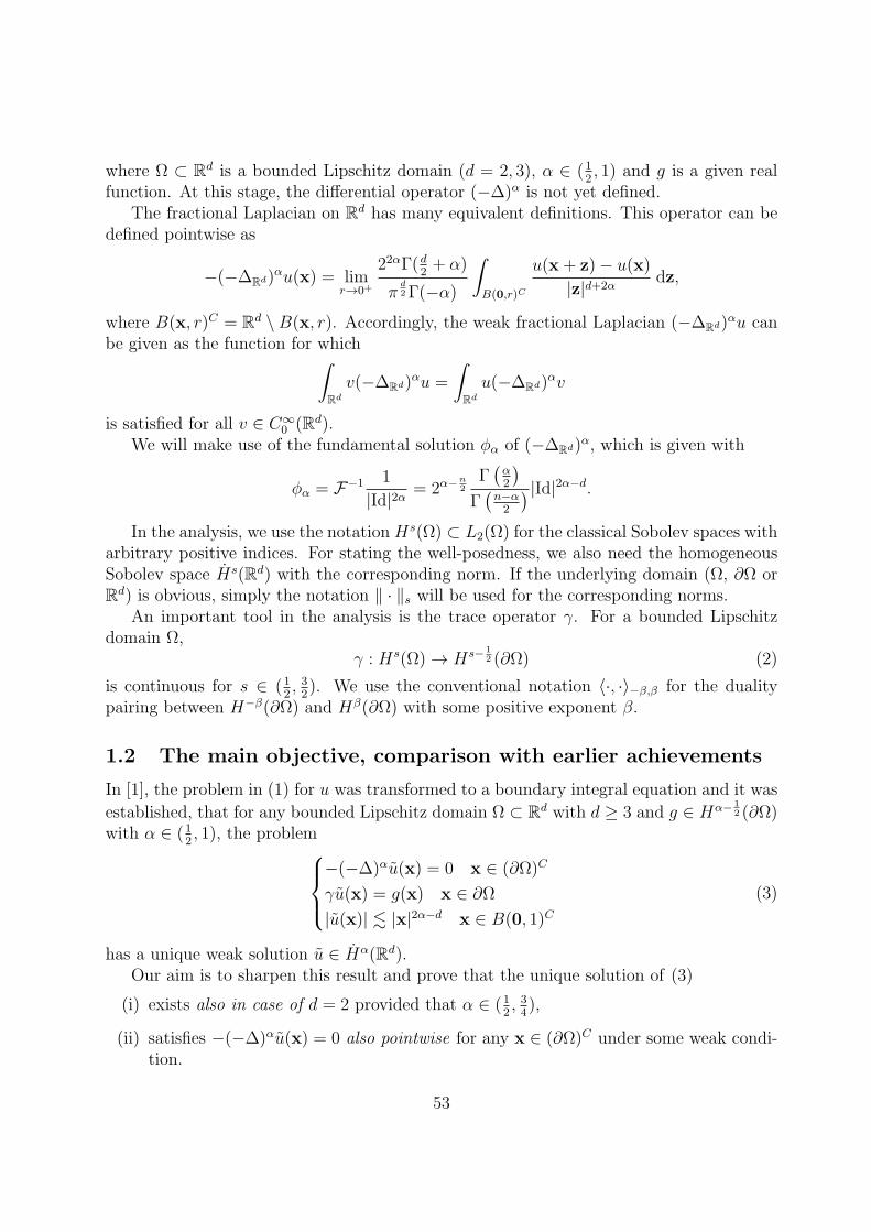
where Ω ⊂ Rd is a bounded Lipschitz domain (d = 2, 3), α ∈ (1

2, 1) and g is a given real

function. At this stage, the differential operator (−∆)α is not yet defined.The fractional Laplacian on R

d has many equivalent definitions. This operator can bedefined pointwise as

−(−∆Rd)αu(x) = limr→0+

22αΓ(d2+ α)

πd2Γ(−α)

∫

B(0,r)C

u(x+ z)− u(x)

|z|d+2αdz,

where B(x, r)C = Rd \ B(x, r). Accordingly, the weak fractional Laplacian (−∆Rd)αu can

be given as the function for which∫

Rd

v(−∆Rd)αu =

∫

Rd

u(−∆Rd)αv

is satisfied for all v ∈ C∞0 (Rd).

We will make use of the fundamental solution φα of (−∆Rd)α, which is given with

φα = F−1 1

|Id|2α= 2α−

n2

Γ(

α2

)

Γ(

n−α2

) |Id|2α−d.

In the analysis, we use the notationHs(Ω) ⊂ L2(Ω) for the classical Sobolev spaces witharbitrary positive indices. For stating the well-posedness, we also need the homogeneousSobolev space Hs(Rd) with the corresponding norm. If the underlying domain (Ω, ∂Ω orR

d) is obvious, simply the notation ‖ · ‖s will be used for the corresponding norms.An important tool in the analysis is the trace operator γ. For a bounded Lipschitz

domain Ω,γ : Hs(Ω) → Hs− 1

2 (∂Ω) (2)

is continuous for s ∈ (12, 32). We use the conventional notation 〈·, ·〉−β,β for the duality

pairing between H−β(∂Ω) and Hβ(∂Ω) with some positive exponent β.

1.2 The main objective, comparison with earlier achievements

In [1], the problem in (1) for u was transformed to a boundary integral equation and it was

established, that for any bounded Lipschitz domain Ω ⊂ Rd with d ≥ 3 and g ∈ Hα− 1

2 (∂Ω)with α ∈ (1

2, 1), the problem

−(−∆)αu(x) = 0 x ∈ (∂Ω)C

γu(x) = g(x) x ∈ ∂Ω

|u(x)| . |x|2α−d x ∈ B(0, 1)C(3)

has a unique weak solution u ∈ Hα(Rd).Our aim is to sharpen this result and prove that the unique solution of (3)

(i) exists also in case of d = 2 provided that α ∈ (12, 34),

(ii) satisfies −(−∆)αu(x) = 0 also pointwise for any x ∈ (∂Ω)C under some weak condi-tion.

53

2 Main results

Assume that α ∈ (0, 1) for d = 3 or α ∈ (12, 34) for d = 2. We investigate the surface

potential, which is given for any x ∈ Rd with

Sα(u)(x) =

∫

∂Ω

φα(x− y)u(y) dy. (4)

In precise terms, in [3] we state the following generalization of (4.1) in [1].For any indices s, α satisfying the assumptions above and 2α− s ∈ (1

2, 32), the mapping

Sα defines a continuous linear operator between Hs−2α+ 1

2 (∂Ω) and Hs(Ω), i.e. for all

ψ ∈ Hs−2α+ 1

2 (∂Ω), we have‖Sα(ψ)‖s . ‖ψ‖s−2α+ 1

2,∂Ω. (5)

We also show that the map γSα is a coercive operator between H1/2−α(∂Ω) andHα−1/2(∂Ω) in the sense that

〈u, γSαu〉 1

2−α,α− 1

2

=

∫

∂Ω

(Sαu)(x)u(x) dx & ‖u‖21/2−α,∂Ω. (6)

Using inequalities (5),(6) and the continuity of the trace operator γ, we can prove our

main statement, that is for any g ∈ Hα− 1

2 (∂Ω), there is a unique function G ∈ H1

2−α(∂Ω),

that solves the equationγSα(G) = g

which yields that u = Sα(G) ∈ Hα(Rd) solves the problem in (3).If, we have additionally G ∈ L1(∂Ω), then the pointwise equality −(−∆)αu = 0 in (∂Ω)C

is also satisfied.Since we showed the coercivity of operator γSα, we can formulate an appropriate form

of Cea-lemma, and use a Galerkin boundary element method to simulate the problem. LetGh ∈ S0

h(∂Ω) be the unique solution to

〈vh, γSα(G−Gh)〉1/2−α,α−1/2 = 0 ∀vh ∈ S0h(∂Ω)

where S0h(∂Ω) is the space of piecewise constant functions defined on an appropriate tri-

angulation (Γj)j∈1...k of ∂Ω with maximal diameter h. If we reconstruct the approximatesolution uh from Gh, for s ∈ [1/2− α, 1] we get the a priori estimate

‖u− uh‖α,Rn .∑

Γj∈∂Ω

hs−(1/2−α)‖G‖s,Γj.

Acknowledgments

The project has been supported by the European Union, co-financed by the EuropeanSocial Fund (EFOP-3.6.3-VEKOP-16-2017-00002). This work was completed in the ELTEInstitutional Excellence Program (1783-3/2018/FEKUTSRAT) supported by the Hungar-ian Ministry of Human Capacities.

54

References

[1] Chang, T. Boundary integral operator for the fractional Laplace equation in a boundedLipschitz domain, INTEGR EQUAT OPER TH, 72(3), 345-361, 2012.

[2] Du, Q. and Gunzburger, M. and Lehoucq, R. B. and Zhou, K. A nonlocal vectorcalculus, nonlocal volume-constrained problems, and nonlocal balance laws, Math. Mod.

Meth. Appl. Sci., 23(3), 493-540, 2013.

[3] Izsak, F. and Maros, G. Fractional order elliptic problems with inhomogeneous Dirichletboundary conditions, Fract. Calc. Appl. Anal., accepted for publication

55

On computation of the matrix Mittag-Leffler function

Ivan Matychyn1, Viktoriia Onyshchenko2

1University of Warmia and Mazury in Olsztyn, Poland2State University of Telecommunications, Ukraine

The theory of fractional differential equations is a new and important branch of dif-ferential equation theory, which has numerous applications and provides realistic modelsfor many real-life processes and phenomena. The Mittag-Leffler function Eα,β(z) playsthe same role in fractional differential equations that the exponential function ez plays inordinary differential equations.

A natural extension of the exponential function to the case of matrix arguments provedto be extremely useful in studying the linear systems of ordinary differential equationsarising in engineering, mechanics, control theory etc. Similarly the matrix Mittag-Lefflerfunction is crucial in linear systems of fractional differential equations, allowing to representexplicitly their solutions. That is why the methods for computing the matrix Mittag-Lefflerfunction are so important.

There exists a wide range of methods for computing of the matrix exponential and manyof them can be adapted for computation of the matrix Mittag-Leffler function. One of themethods is based on Jordan canonical form [8]. Here we apply this approach and propose atechnique for computation the matrix Mittag-Leffler function, which is implemented withMatlab code [7].

The numerical methods based on Jordan canonical form have major disadvantage,since the involved similarity transformation can be ill-conditioned. However the numericalexperiments on the benchmark example of the Bagley–Torvik equation [1] imply that theproposed approach allows to obtain satisfactory accuracy.

The matrix Mittag-Leffler function was probably first introduced in the paper [2], whereit was used in an explicit solution of a linear system of fractional order equation (FDEs)

Dαz = Az + f, 0 < α ≤ 1. (1)

Here Dαz stands for the Riemann–Liouville fractional derivative of order α [5]. Ingeneral, if g is a function having absolutely continuous derivatives up to the order m− 1,the Riemann–Liouville derivative of fractional order α, m− 1 < α ≤ m, can be defined asfollows:

Dαg(t) =1

Γ(m− α)

dm

dtm

∫ t

0

g(τ)

(t− τ)α−m+1dτ.

Hereafter A is a fixed real n × n matrix, and z, f : [0,∞) → Rn are measurable

vector-functions taking values in Rn.

56

If (1) is supplied with initial condition of the form

1

Γ(1− α)

∫ t

0

z(τ)

(t− τ)αdτ

∣

∣

∣

t=0

= z0, (2)

then solution to the initial value problem (1), (2) can be written down in the form [3]

z(t) = tα−1Eα,α(Atα)z0 +

∫ t

0

(t− τ)α−1Eα,α(A(t− τ)α)f(τ)dτ, (3)

where

Eα,β(A) =∞∑

k=0

Ak

Γ(αk + β), α > 0, β ∈ C, (4)

denotes the matrix Mittag-Leffler function of A.The explicit expression (3) plays a key role in numerous applications related to systems

with fractional dynamics [6]. That is why the methods for computing the matrix Mittag-Leffler function are so important.

Both the matrix Mittag-Leffler function and the matrix α-exponential functions aregeneralizations of matrix exponential function, since

E1,1(At) = eAt1

= eAt.

This implies that some of numerous existing methods for computing the matrix exponentialcan be adapted for the matrix Mittag-Leffler functions as well. An overview and analysisof these methods can be found in the paper [8].

There exists a number of equivalent definitions of a matrix function. The followingdefinition [4] is based on the Jordan canonical form. We will use the latter for computingthe matrix Mittag-Leffler function.

Definition 1 (matrix function via Jordan canonical form). Let the function f be definedon the spectrum of A and let A = ZJZ−1, where J is the Jordan canonical form. Then

f(A) = Zf(J)Z−1 = Z diagf(J1), f(J2), . . . , f(Js)Z−1, (5)

where

f(Jk) =

f(λk) f ′(λk)f ′′

(λk)

2. . .

f (mk−1)

(λk)

(mk−1)!

0 f(λk) f ′(λk) . . .f (m

k−2)

(λk)

(mk−2)!

0 0 f(λk) . . .f (m

k−3)

(λk)

(mk−3)!

......

.... . .

...0 0 0 . . . f ′(λk)0 0 0 . . . f(λk)

. (6)

57

The generalized (scalar) Mittag-Leffler function also known as Prabhakar function isdefined for complex z, α, β, ρ ∈ C, and ℜ(α) > 0 by

Eρα,β(z) =

∞∑

k=0

(ρ)kΓ(αk + β)

zk

k!,

where (ρ)k = ρ(ρ+ 1) . . . (ρ+ k − 1) is the Pochhammer symbol.In particular, when ρ = 1, it coincides with the Mittag-Leffler function (4):

E1

α,β(z) = Eα,β(z).

Since the expression (6) involves derivatives, the following equation [5] is important forthe purpose of computing the matrix Mittag-Leffler function:

(

d

dt

)m

Eα,β(t) = m!Em+1

α,β+αm(t), m ∈ N. (7)

In view of (7), the formulas (5), (6) take on the form

Eα,β(A) = Z diagEα,β(J1), Eα,β(J2), . . . , Eα,β(Js)Z−1, (8)

Eα,β(Jk)

=

Eα,β(λk) E2

α,β+α(λk) . . . Em

k

α,β+(mk−1)α(λk)

0 Eα,β(λk) . . . Em

k−1

α,β+(mk−2)α(λk)

0 0 . . . Em

k−2

α,β+(mk−3)α(λk)

......

. . ....

0 0 . . . E2

α,β+α(λk)0 0 . . . Eα,β(λk)

.(9)

The method of computing the matrix Mittag-Leffler function based on the Jordan canonicalform representation (8), (9) is implemented with Matlab code [7].

References

[1] R.L. Bagley and P.J. Torvik, On the appearance of the fractional derivative in thebehavior of real materials, J. Appl. Mech., 51 (2), 294-298 (1984).

[2] A.A. Chikrii, S.D. Eidelman, Generalized Mittag-Leffler matrix functions in game

problems for evolutionary equations of fractional order, Cybernetics and SystemsAnalysis, 36(3):315–338, 2000.

[3] A.A. Chikriy, I.I. Matichin. Presentation of solutions of linear systems with frac-

tional derivatives in the sense of Riemann–Liouville, Caputo, and Miller–Ross, J. ofAutomation and Information Sciences, 40(6):1–11, 2008.

58

[4] F.R. Gantmacher, Teoria matric, Nauka, Moskwa 1967.

[5] A.A. Kilbas, H.M. Srivastava, J.J. Trujillo, Theory and Applications of Fractional

Differential Equations, Elsevier, Amsterdam, 2006.

[6] I. Matychyn and V. Onyshchenko, Time-optimal control of fractional-order linear sys-tems, Fractional Calculus and Applied Analysis, 18 (3), 687-696 (2015).

[7] I. Matychyn, Matrix Mittag-Leffler function, MATLAB Central File Exchange, FileID: 62790 (2017).

[8] C. Moler and C. Van Loan, Nineteen dubious ways to compute the exponential of amatrix, twenty-five years later, SIAM review, 45 (1), 3-49 (2003).

59

Implementation of fractional optimal control problems

in real-world applications

Neelam Singha

Pandit Deendayal Petroleum University Gandhinagar, India

The present work intends to discuss various practical applications of fractional calculus.

Specifically, we have analyzed the need of fractional-order operators in formulating various

cancer-tumor models. Modelling of such systems with non-local memory preserving frac-

tional derivatives enables us to describe the dynamics of tumor-immune interactions. The

underlying motive is to review these models as fractional optimal control problems and

perform suitable investigation.

60

Nested dissection reordering in a HSS solver for

fractional diffusion problems

D. Slavchev, S. MargenovInstitute of Information and Communication Technologies,

Bulgarian Academy of Sciences

1 Introduction

The anomalous diffusion (fractional diffusion) is a process where the relationship betweenmean square displacement and time is not linear. It has a wide range of applications in mod-eling transport within cells, in porous materials, ion channels in plasma membrane, atmo-spheric processes and others. The fractional diffusion operators and the related boundaryvalue problems are non-local, thus resulting in dense systems of linear algebraic equations.Solving such systems with Gaussian elimination is computationally too expensive. Un-der certain assumptions, the Hierarchical compression methods offer better computationalcomplexity. Initially developed for boundary element discretizations, they are also applica-ble to the fractional Laplacian defined through the Ritz potential. However the efficiencyof the compression is highly dependent on the structure of the underlying matrix. Bygood structure we understand the existence of approximately low-rank off-diagonal blocks,which depends on the ordering of the unknowns. In this work we are interested in applyingthe reordering provided by the Nested Dissection algorithm when using Hierarchical Semi-Separable compression for a fractional diffusion problem. The performance of the resultingsolver is analyzed.

2 Fractional diffusion

Let us consider the fractional Laplacian defined through the Ritz potential:

(−∆)α u (x) = C (n, α) p.v.∫

IRn

u (x)− u (y)

|x− y|n+2αdy, α ∈ (0, 1) , (1)

where p.v. stands for principal value, C is the normalized constant

C (n, α) =22ααΓ

(

α + n2

)

πn/2Γ (1− α),

61

n is the dimension, Γ is the Gamma function, and Ω is a bounded domain. We considerthe homogeneous Dirichlet problem associated with (1):

(−∆)α u = f, x ∈ Ω,u = 0, x /∈ Ω.

The 2D finite element discretization presented in [1] is used in this study. The efficiencyof the hierarchical solver is analyzed for test linear systems corresponding to square andcircle domain Ω.

3 STRUMPACK solver

The STRUctured Matrix PACKage (STRUMPACK) is a parallel library providing compu-tational routines for structured matrices – i.e. matrices that exhibit some low-rank property(sparse matrices and dense rank-deficient matrices). We are interested in the implemen-tation of the Hierarchical Semi-Separable (HSS) compression solver [2]. Solving a systemAx = b with HSS compression includes 3 steps:

1. HSS compression: A is compressed into a HSS form H using random sampling. Thisis done recursively by first dividing the matrix in 4 square blocks, expressing theoff-diagonal blocks as a product of three matrices (U , B (small and square) and V )called generators.

A =

[

A11 A12

A21 A22

]

, Aij,i 6=j = Ubigi BijV

bigj

∗

.

The blocks Aii are recursively compressed in a similar way. The computationalcomplexity is O(r2n), where n is the number of unknowns and r is the calculatedmaximum rank of the off-diagonal blocks.

2. ULV-like factorization: Changes the variables from x to y, and solves the systemin two passes. The first one solves O(n − r) unknowns using the structure of H,and the second pass solves the rest O(r) unknowns with Gaussian elimination. Thecomputational complexity is O(r2n).

3. Solution: Finds the solution x from the solution y obtained at the second step. Thecomputational complexity is O(rn).

4 Nested Dissection Reordering

The ordering of the unknowns is important for the efficiency of the hierarchical algorithm.The ordering produced by the MATLAB code in [1] results in a poor compression. In [4, 3]we have analyzed several reordering schemes. The goal of this work is to investigate the

62

use of the Nested Dissection (ND) algorithm for this purpose. The ND [5] is developed toreduce the fill-ins of Gaussian elimination of sparse matrices. It uses a divide and conquer

strategy on the graph of the matrix. The selection of a set of vertices (separator) dividesthe matrix into a 3×3 (or more) block structure. The algorithm is applied recursively. Thefractional diffusion matrix is dense, however, and ND wouldn’t help solving it with Gaussianelimination. Here, the ND reordering is applied to the HSS compression solver aimedat reducing the rank of the off-diagonal blocks, and thus increasing the computationalefficiency.

Acknowledgments

The partial support through the Grant No BG05M2OP001-1.001-0003, financed by the Sci-ence and Education for Smart Growth Operational Program (2014-2020) and co-financedby the EU through the European Structural and Investment Funds, and through the Bul-garian NSF Grant No DFNI-DN12/1 is highly appreciated.

References

[1] Acosta, G., Bersetche, F., Borthagaray, J.: A short FE implementation for a 2D homo-geneous Dirichlet problem of a Fractional Laplacian, Comput. Math. Appl., 8 (2017),784–816

[2] Rouet, F.-H., Li, X.S., Ghysels, P., Napov, A.: A Distributed-Memory Packagefor Dense Hierarchically Semi-Separable Matrix Computations Using Randomization,ACM Trans. Math. Softw., 42(4) (2016), 1–27

[3] Slavchev, D.: On the impact of reordering in a hierarchical semi-separable compres-sion solver for fractional diffusion problems, Large-Scale Scientific Computing, Springer

LNCS 11958 (2020), 373–381

[4] Slavchev, D., Margenov, S.: Performance analysis of hierarchical semi-separable com-pression solver for fractional diffusion problems, Advanced Computing in Industrial

Mathematics, Springer Cham, in press

[5] George, A.: Nested dissection of a regular finite element mesh, SIAM Num. Anal. 10(2)

(73), 345–363

63

A survey on fast algorithms for fractional diffusion

equations and its applications

HongGuang Sun, Xiaoting LiuState Key Laboratory of Hydrology-Water Resources

and Hydraulic Engineering,College of Mechanics and Materials,

Hohai University, China

Fractional diffusion equations (FDEs), which are well known as a valid model capturinganomalous diffusion due to its memory and long range interaction, have been successfullyapplied to simulate the transportation process of contaminant in the underground wa-ter. The objective of our works is to provide fast algorithms and develop the meshlessmethod (Kansa method) to dealwith the fractional diffusion equations with arbitrary an-gle in two dimension. For the fast algorithms on time fractional calculus, we proposed thesemi-discrete method together with scale-dependent difference method, separately. Sub-sequently, we numerically solve the variable-order vector fractional-derivative models tosimulate multi-dimensional anomalous diffusion in nonstationary media. Hence, our workcan provide a fast and convenient tool to quantify complex anomalous transport in multi-dimensional and non-stationary media with continuously or abruptly changing heterogene-ity, filling the knowledge gap in parsimonious non-local transport models developed in thelast decades.

Contaminant transport modeling has been the prerequisite for many environmentalprotection applications, but efficiently predicting real-world mass transport remains a his-torical challenge for the geophysical and hydrological communities. The physical hetero-geneity of natural geological media with intrinsic scale effects has been well recognized asthe major mechanism of anomalous diffusion, but it cannot be measured exhaustively at allrelevant scales. It is well-known that traditional second-order diffusion models built uponthe standard Fick’s law cannot efficiently capture non-Fickian features of mass transportprocesses. These features include apparent early-arrivals and/or heavy late-time tailing incontaminant breakthrough curves, as well as scale-dependent transport coefficients. Thefailure of second-order diffusion equations in capturing non-Fickian transport has moti-vated the application of time and space fractional-order diffusion equations (FDEs) tocontaminant transport in porous media.

Although the FDE models have been successfully used to capture anomalous diffusionin the last several decades, efficient numerical solvers for the FDEs are still required for

64

engineering applications that involve large, geometrically complex spatial domains andlong-time range predictions. The need for these solvers stems from two reasons. First, thetime fractional derivative in the FDE retains a memory of its entire history. Comparedwith the integer-order derivative which is a local operator, the computational cost of thetemporal FDE dramatically increases with the total modeling time. Second, although theglobal correlation defined by the space fractional derivative (especially the fractional Lapla-cian operator) enables the FDE to characterize the spatial non-local nature of contaminanttransport, it causes a computational challenge in approximating spatial FDEs using thegrid-based finite difference method (FDM) or finite element method (FEM). Because thefractional derivative is a non-local operator, the parameter matrix in the FDM (or thestiffness matrix in the FEM) for FDEs is not banded or sparse (as is the standard diffusionequation), but almost dense. This issue challenges the accuracy and efficiency of numericalapproximations for high-dimensional space FDEs. Previous studies focusing on FDM andFEM methods have provided various accurate and mathematical convergent schemes forsolving space FDE models, but the prohibitive computational cost challenges long-rangetime computation of the spatiotemporal FDEs in large spatial domains.

Vector FDEs are needed to capture real-world diffusion in multi-dimensional media. Anextension of FDEs from one dimension to two or three dimensions is not as straightforwardas that for the second-order diffusion equation, due to the global correlation nature ofanomalous transport. Meerschaert et al. proposed a vector fractional derivative as ageneralization of the Laplacian term, which satisfies the global correlation property andcan efficiently describe anomalous transport in complex media with preferential flow path.Therefore, we adopt their definition and focus on the development of numerical methodsfor solving spatiotemporal FDEs containing the vector fractional derivative operator.

In addition, real-world anomalous diffusion can cover a large domain, challenging classi-cal grid-based numerical solvers such as the FDM. The computational cost of the FEM onmesh generation and assembling of the asymmetric stiffness matrix also increases dramat-ically. The radial basis function (RBF) collocation technique, which is a global meshlessmethod, was recognized as an efficient method to approximate the differential equationsin large and irregular domains. The RBF method has also proved to be a meshless meritmethod with the advantages of high accuracy and ease of implementation in discretizingthe space-fractional derivative.

For the fast algorithms on time fractional calculus, we proposed the semi- discretemethod and scale-dependent difference method, separately. On one hand, we proposeda semi-discrete method, in which an exact solution for the ODE was obtained using theanalytical technique and property of the Mittag-Leffler function, to approximate the timefractional derivative term achieving a fast and accurate solution. On the other hand, weproposed a scale-dependent finite difference method (S-FDM) to approximate the timefractional differential equations (FDEs), using Hausdroff metric to conveniently link theorder of the time fractional derivative (α) and the non-uniform time intervals. Consideringthe complex spatial structure in geological media, we developed, evaluated, and appliedvariable-order, vector, spatial fractional-derivative equation (FDE) models with a Kansasolver, to capture spatiotemporal variation of super-diffusion along arbitrary angles (i.e.,

65

preferential pathways). Those studies aim at providing an efficient method which cansolve the spatiotemporal FDE in large, two-dimensional spatial domains, and provide along-time range prediction of anomalous pollutant transport.

References

[1] Liu, X.T., Sun, H.G., Zhang, Y., Zheng, C., Yu, Z.: Simulating multi-dimensionalanomalous diffusion in nonstationary media using variable-order vector fractional-derivative models with Kansa solver, Adv. Water Resour. 133 (2019), 103423

[2] Liu, X.T., Sun, H.G., Zhang, Y., Fu, F.: A scale-dependent finite difference approxi-mation for time fractional differential equation, Comput. Mech. 63(3) (2019), 429–442

[3] Sun, H.G., Liu, X.T., Zhang, Y., Pang, G., Garrard, R..: A fast semi-discrete Kansamethod to solve the two-dimensional spatiotemporal fractional diffusion equation, J.Comput. Phys. 345 (2017), 74–90

[4] Sun, H.G., Chen, W., Sze, K.Y.: A semi-discrete finite element method for a class oftime-fractional diffusion equations, Philos. T. R. Soc. A. 371 (2013), 20120268

66

Approximate representation of the solutions of

fractional elliptical BVP through the solution of

parabolic IVP

Petr N. VabishchevichNuclear Safety Institute of RAS, RussiaNorth-Eastern Federal University, Russia

Boundary value problem for a fractional power of an elliptic operator is considered.To solve such problems we use an integral representation by means of a standard solutionproblem for parabolic equations.

Problem formulation. Introduce the elliptic operator as

Av = −div(a(x)grad v) + c(x)v, x ∈ Ω, (1)

with coefficients 0 < a1 ≤ a(x) ≤ a2, c(x) ≥ 0. The operator A is defined on the set offunctions v(x) that satisfy on the boundary ∂Ω the following conditions:

v(x) = 0, x ∈ ∂Ω. (2)

In the Hilbert space H = L2(Ω), we define the scalar product and norm in the standardway:

(v, w) =∫

Ωv(x)w(x)dx, ‖v‖ = (v, v)1/2.

In the spectral problem

Aϕk = λkϕk, x ∈ Ω, ϕk = 0, x ∈ ∂Ω,

we have 0 < λ1 ≤ λ2 ≤ ..., and the eigenfunctions ϕk, ‖ϕk‖ = 1, k = 1, 2, ... form a basis

in H. Therefore, v =∞∑

k=1

(v, ϕk)ϕk. Let the operator A be defined in the following domain:

D(A) =

v | v(x) ∈ L2(Ω),∞∑

k=0

|(v, ϕk)|2λk < ∞

.

Under these conditions A : H → H and the operator A is self-adjoint and positive definite:

A = A∗ ≥ νI, ν > 0, (3)

67

where I is the identity operator in H. In applications, the value of λ1 is unknown (thespectral problem must be solved). Therefore, we suppose that ν ≤ λ1 in (3). Let us assumefor the fractional power of the operator A:

Aαv =∞∑

k=0

(v, ϕk)λαkϕk.

The solution v(x) satisfies the equation

Aαv = f (4)

under the restriction 0 < α < 1.Representation through parabolic IVP solutions. An approximate solution to

the boundary value problem for the fractional degree of an elliptic operator (4) often basedon the use of one or another integral representation. For example, in the works A. Bonito,J. E. Pasciak (2016), L. Aceto, P. Novati (2017) the Balakrishnan formula is used when

A−α =sin(πα)

π

∫

∞

0θ−α(A+ θI)−1dθ, 0 < α < 1. (5)

The approximation of A−α is based on the use of one or another quadrature formulas forthe right-hand side of (5).

On this path, the possibilities of approximating both the fractional power of the oper-ator A−α and approximating the solution of the problem are realized.

1. Rational function approximation A−α:

A−α ≈m∑

i=1

γi(A+ θiI)−1,

where γi > 0 are the weights, and θi > 0, i = 1, 2, . . . ,m are the nodes of thequadrature formula for (5).

2. An approximate solution to the problem (4):

v ≈m∑

i=1

γivi, (A+ θiI)vi = f, i = 1, 2, . . . ,m.

The inverse operator of the fractional power elliptic problem is treated as a sum of in-verse operators of classical elliptic operators, and required an approximate solution of theproblem as the sum of the solutions of standard elliptical BVP.

The integral representation of the fractional power of the elliptic operator, which isfundamentally different from (5) used in works N. Cusimano, F. del Teso, L. Gerardo-Giorda, G. Pagnini (2018), N. Cusimano, F. del Teso, L. Gerardo-Giorda (2018). It is

68

based on the method of semigroups, A−α is defined through an integral formulation asfollows

A−α =1

Γ(α)

∫

∞

0θα−1e−θAdθ, 0 < α < 1, (6)

where Γ(α) is gamma function. In this case, the solution to the problem (4) is

v =1

Γ(α)

∫

∞

0θα−1e−θAf dθ. (7)

Function w(t) = e−tAf is a solution of the following Cauchy problem

dw

dt+ Aw = 0, 0 < t < ∞, (8)

w(0) = f. (9)

By the representation (7) we have

v =1

Γ(α)

∫

∞

0θα−1w(θ)dθ. (10)

For (1), (2) the problem (8), (9) is the standard Cauchy problem for a second-orderparabolic equation. Based on (10), the fractional elliptical BVP solution is representedthrough the solution IVP for the parabolic equation.

We note the most important features of the approximation of the fractional power ofthe operator A−α and solving the problem (4) based on the integral representation (6).

1. Using quadrature formulas for (6) we come to the approximation A−α with operatorexponentials:

A−α ≈m∑

i=1

γie−θiA.

Here, as before, γi > 0, θi > 0, i = 1, 2, . . . ,m there are weights and nodes corre-sponding quadrature formula.

2. For an approximate solution to the problem (4) from (10) we have

u ≈ um =m∑

i=1

γiw(θi), (11)

where w(t) is the solution to the problem (8), (9).

Thus, the computational algorithm for solving the problem (4) can be built on a nu-merical solution of the Cauchy problem (8), (9), according to which, in accordance withthe selected quadrature formula (see (11)) we have approximate solution. Approximationsof the desired solution fractional elliptical BVP is based on generalized Gauss-Laguerreformula, which most fully takes into account the singularity of the integral representation.

69

Subdiffusion with a time-dependent coefficient:

analysis and numerical approximation

Zhi ZhouDepartment of Applied Mathematics,Hong Kong Polytechnic University

The aim of this work is to study the subdiffusion equation with a time-dependentdiffusion coefficient, by using a perturbation argument [7, 8]. Let Ω ⊂ R

d (d ≥ 1) bea convex polyhedral domain with a boundary ∂Ω. Consider the following fractional-order parabolic problem for the function u(x, t):

∂αt u(x, t)− A(x, t)u(x, t) = f(x, t) (x, t) ∈ Ω× (0, T ],

u(x, t) = 0 (x, t) ∈ ∂Ω× (0, T ],

u(x, 0) = u0(x) x ∈ Ω,

(1)

where T > 0 is a fixed final time, f and u0 are given source term and initial data,respectively. We assume that A(x, t)u = ∇·(a(x, t)∇u), where the diffusion coefficientmatrix a(x, t) : Ω×(0, T ] → R

d×d is symmetric and smooth, and satisfies the ellipticitycondition. The notation ∂α

t u(t) denotes the left-sided Caputo derivative of order α ∈(0, 1), defined by [9, p. 70]

∂αt u(x, t) =

1

Γ(1− α)

∫ t

0

(t− s)−α∂su(x, s)ds. (2)

The literature on the numerical analysis of the subdiffusion problem is vast; seethe overview [5] (and the references therein). However, most of these works analyzedonly the case that the diffusion coefficient a is independent of the time t. These worksmostly employ Laplace transform and its discrete analogue for analysis, which are notdirectly applicable to the case of a time-dependent coefficient.

For standard parabolic problems with a time-dependent coefficient, there are a fewrelevant works [10, 12, 15, 16]. Unfortunately, the fractional derivative does not sat-isfy the well known Leibnitz rule. Hence, some traditional techniques working for heatequation cannot be directly applied here, and the analysis of fractional diffusion withtime-dependent coefficients and its numerical approximation remain fairly challeng-ing. Very recently, Mustapha [13] analyzed the spatially semidiscrete Galerkin FEMapproximation of problem (1) using a novel energy argument, and established optimal-order convergence rates for both smooth and nonsmooth initial data. However, thework [13] did not discuss the source term and the analysis is under certain regularityassumptions on the solution, which have not been rigorously established yet.

In particular, we assume that

v ∈ L2(Ω) and

∫ t

0

(t− s)α−1‖ft(s)‖L2(Ω) ds < 0. (3)

70

In general, the solution of (1) is not smooth under these conditions.To discretize the problem, let Th be a shape regular quasi-uniform triangulation

of the domain Ω, with the maximal diameter h, and Sh ⊂ H10 (Ω) be the space of

continuous piecewise linear functions on the triangulation Th. Let Ah(t) : Sh → Sh bethe discrete diffusion operator defined via duality [12]. Then the spatial semidiscretescheme reads: find uh(t) ∈ Sh such that

∂αt uh(t) + Ah(t)uh(t) = fh(t) := Phf(t), ∀ t ∈ (0, T ], (4)

with uh(0) = vh := Phv, where Ph denotes the L2-projection operator. Further, let ∂ατ

be the discrete fractional time derivative by the CQ generated by the backward Eulermethod [11]. Then the fully discrete scheme reads: find Un

h ∈ Sh such that

∂ατ (U

nh − u0

h) + Ah(tn)Unh = Phf(tn), n = 1, 2, . . . , N, (5)

with U0h = vh. We shall prove the error estimate that

‖Unh − u(tn)‖L2(Ω) ≤ c(h2 log(1 + 1/h)t−α

n + τ log(1 + tn/τ)t−1n ) (6)

under the regularity assumption (3). The logarithmic factors appear due to the singu-larity of the solution and the application of discrete Gronwall’s inequality. If the dif-fusion operator is independent of time, the error estimate was given in [4] via Laplacetransform, which is not applicable to the time-dependent case under consideration.Our basic strategy is to combine the existing estimates in [3, 2, 4] with a novel per-turbation argument.

Specifically, we can reformulate the problem for any t0 ∈ (0, T ] as

∂αt u(t) + A(t0)u(t) = (A(t0)− A(t))u(t) + f(t), t ∈ (0, T ],

Then the solution can be expressed by

u(t) = E(t; t0)v +

∫ t

0

E(t− s; t0)(f(s) + (A(t0)− A(s))u(s)) ds, (7)

where the solution operators E(t; t0) and E(t − s; t0) are well understood [14]. Nowthe desired regularity of the solution will follow from several perturbation estimates ofthe diffusion operator, the smoothing property of the operators E(t; t0) and E(t; t0),the fixed point theorem and a generalized Gronwall’s inequality.

This perturbation strategy is expected to be applicable to analyze the semidiscretescheme (4). Specifically, the solution uh of problem (4) can be represented by (adiscrete analogue to (7))

uh(t) = Eh(t; t0)Phv +

∫ t

0

Eh(t− s; t0)(

Phf(s) + (Ah(t0)− Ah(s))uh(s))

ds, (8)

where the semidiscrete operators Eh(t; t0) and Eh(t; t0) were thoroughly studied in[3, 2]. Let eh = Phu − uh. Then it follows from (7) and (8) that eh can be expressedby

eh(t) =(PhE(t; t0)− Eh(t; t0)Phv) +

∫ t

0

(PhE(t− s; t0)− Eh(t− s; t0)Ph)f(s)ds

+

∫ t

0

(PhE(t− s; t0)− Eh(t− s; t0)Ph)(A(t0)− A(s))u(s)ds

+

∫ t

0

Eh(t− s; t0)(

(PhA(t0)− PhA(s))u(s)− (Ah(t0)− Ah(s))uh(s))

ds

71

The first and second terms can be bounded by the regularity estimates and existingresults in [3, 2]. The third and fourth terms follow analogously with some additionalperturbation properties of the semidiscrete diffusion operator Ah(t) and the corre-sponding Ritz projection operator. These together with Gronwall’s inequality implythe error estimates.

To study the fully discrete scheme (5), it is crucial to derive the temporal regularityof the solution u. In particular, for CQ generated by backward Euler method, it issufficient to prove that ‖∂tu(t)‖L2(Ω) ≤ ct−1 under the assumption (3). Then the per-turbation argument, together with approximation properties of fully discrete solutionoperators and discrete Gronwall inequality, yields the desired error estimate (6).

Finally, we shall extend the perturbation argument to high-order time steppingschemes of subdiffusion equations with time-dependent diffusion coefficients. In [8], wepropose a second-order time-stepping scheme for problem (1) with nonsmooth initialdata and incompatible source term. It is based on the CQ generated by the second-order backward differentiation formula (BDF2), with suitable correction at the firststep. The correction is inspired by the recent works [1, 4, 6] and essential for restoringthe second-order convergence. We prove the a convergence rate O(τ 2) for any fixedtn > 0, of the scheme for both nonsmooth initial data and incompatible source term.The error analysis relies heavily on new temporal regularity results for the model (1)and a refined perturbation argument, which substantially extends the prior work [7].

Numerical experiments are consistent with the theoretical results.

References

[1] E. Cuesta, C. Lubich, and C. Palencia. Convolution quadrature time discretizationof fractional diffusion-wave equations. Math. Comp., 75(254):673–696, 2006.

[2] B. Jin, R. Lazarov, J. Pasciak, and Z. Zhou. Error analysis of semidiscrete finiteelement methods for inhomogeneous time-fractional diffusion. IMA J. Numer.

Anal., 35(2):561–582, 2015.

[3] B. Jin, R. Lazarov, and Z. Zhou. Error estimates for a semidiscrete finite ele-ment method for fractional order parabolic equations. SIAM J. Numer. Anal.,51(1):445–466, 2013.

[4] B. Jin, R. Lazarov, and Z. Zhou. Two fully discrete schemes for fractional diffu-sion and diffusion-wave equations with nonsmooth data. SIAM J. Sci. Comput.,38(1):A146–A170, 2016.

[5] B. Jin, R. Lazarov, and Z. Zhou. Numerical methods for time-fractional evolutionequations with nonsmooth data: a concise overview. Comput. Methods Appl.

Mech. Engrg., 346:332–358, 2019.

[6] B. Jin, B. Li, and Z. Zhou. Correction of high-order BDF convolution quadraturefor fractional evolution equations. SIAM J. Sci. Comput., 39(6):A3129–A3152,2017.

[7] B. Jin, B. Li, and Z. Zhou. Subdiffusion with a time-dependent coefficient: anal-ysis and numerical solution. Math. Comp., 88(319):2157–2186, 2019.

72

[8] B. Jin, B. Li, and Z. Zhou. Subdiffusion with time-dependent coefficients: im-proved regularity and second-order time stepping. pripret, 2019.

[9] A. A. Kilbas, H. M. Srivastava, and J. J. Trujillo. Theory and Applications of

Fractional Differential Equations. Elsevier Science B.V., Amsterdam, 2006.

[10] H. Lee, J. Lee, and D. Sheen. Laplace transform method for parabolic problemswith time-dependent coefficients. SIAM J. Numer. Anal., 51(1):112–125, 2013.

[11] C. Lubich. Discretized fractional calculus. SIAM J. Math. Anal., 17(3):704–719,1986.

[12] M. Luskin and R. Rannacher. On the smoothing property of the Galerkin methodfor parabolic equations. SIAM J. Numer. Anal., 19(1):93–113, 1982.

[13] K. Mustapha. FEM for time-fractional diffusion equations, novel optimal erroranalyses. Math. Comp., 87(313):2259–2272, 2018.

[14] K. Sakamoto and M. Yamamoto. Initial value/boundary value problems for frac-tional diffusion-wave equations and applications to some inverse problems. J.

Math. Anal. Appl., 382(1):426–447, 2011.

[15] P. Sammon. Fully discrete approximation methods for parabolic problems withnonsmooth initial data. SIAM J. Numer. Anal., 20(3):437–470, 1983.

[16] G. Savare. A(Θ)-stable approximations of abstract Cauchy problems. Numer.

Math., 65(3):319–335, 1993.

73

List of authors

Lidia Aceto, p. 1

University of Pisa, Italy

lidia.aceto@unipi.it

Anatoly A. Alikhanov, p. 3, 6

Institute of Applied Mathematics and Automation, KBSC RAS, Russia

aaalikhanov@gmail.com

Emanouil Atanassov, p. 7

Institute of Information and Communication Technologies,

Bulgarian Academy of Sciences, Bulgaria

emanouil@parallel.bas.bg

Hitesh Bansu, p. 11

Sardar Vallabhbhai National Institute of Technology, India

hiteshbansu@gmail.com

David Bolin, p. 15

King Abdullah University of Science and Technology (KAUST), Saudi Arabia

david.bolin@chalmers.se

Yuri Dimitrov, p. 16

University of Forestry & Institute of Mathematics and Informatics,

Bulgarian Academy of Sciences, Bulgaria

yuri.dimitrov@ltu.bg

Ludmil Drenchev, p. 31

Institute of Metal Science, Equipment and Technologies,

Bulgarian Academy of Sciences, Bulgaria

ljudmil.d@ims.bas.bg

Maria Durchova, p. 7

Institute of Information and Communication Technologies,

Bulgarian Academy of Sciences, Bulgaria

mabs@parallel.bas.bg

Stanislav Harizanov, p. 19, 23

Institute of Information and Communication Technologies,

Bulgarian Academy of Sciences, Bulgaria

sharizanov@parallel.bas.bg

Clemens Hofreither, p. 27

Johann Radon Institute for Computational and Applied Mathematics (RICAM), Austria

clemens.hofreither@ricam.oeaw.ac.at

75

Nevena Ilieva, p. 31

Institute of Information and Communication Technologies,

Bulgarian Academy of Sciences, Bulgaria

nevena.ilieva@parallel.bas.bg

Sofiya Ivanovska, p. 7

Institute of Information and Communication Technologies,

Bulgarian Academy of Sciences, Bulgaria

sofia@parallel.bas.bg

Aneta Karaivanova, p. 7

Institute of Information and Communication Technologies,

Bulgarian Academy of Sciences, Bulgaria

anet@parallel.bas.bg

Ivaylo Katsarov, p. 31

Institute of Metal Science, Equipment and Technologies,

Bulgarian Academy of Sciences, Bulgaria

ivaylo.katsarov@kcl.ac.uk

Aslanbek Kh. Khibiev, p. 6

Institute of Applied Mathematics and Automation, KBSC RAS, Russia

akkhibiev@gmail.com

Virginia Kiryakova, p. 35

Institute of Mathematics and Informatics, Bulgarian Academy of Sciences, Bulgaria

virginia@diogenes.bg

Nikola Kosturski, p. 38

Institute of Information and Communication Technologies,

Bulgarian Academy of Sciences, Bulgaria

kosturski@parallel.bas.bg

Miroslav Kuchta, p. 41

Simula Research Laboratory, Fornebu, Norway

miroslav.kuchta@gmail.com

Maksim V. Kukushkin, p. 45

Moscow State University of Civil Engineering &

Kabardino-Balkarian Scientific Center, RAS, Nalchik, Russia

kukushkinmv@rambler.ru

Sushil Kumar, p. 11

Sardar Vallabhbhai National Institute of Technology, India

skumar.iitr@gmail.com

76

Raytcho Lazarov, p. 19, 23

Texas A&M University, College Station, TX, USA

lazarov@math.tamu.edu

Yingjie Liang, p. 49

Institute of Soft Matter Mechanics, College of Mechanics and Materials,

Hohai University, China

liangyj@hhu.edu.cn

XiaoTing Liu, p. 64

Institute of Soft Matter Mechanics, College of Mechanics and Materials,

Hohai University, China

Svetozar Margenov, p. 19, 23, 38, 61

Institute of Information and Communication Technologies,

Bulgarian Academy of Sciences, Bulgaria

margenov@parallel.bas.bg

Pencho Marinov, p. 19, 23

Institute of Information and Communication Technologies,

Bulgarian Academy of Sciences, Bulgaria

pencho@bas.bg

Gabor Maros, p. 52

ELTE University, Budapest, Hungary

magabor42@gmail.com

Ivan Matychyn, p. 56

University of Warmia and Mazury in Olsztyn, Poland

matychyn@matman.uwm.edu.pl

Viktoriia Onyshchenko, p. 56

State University of Telecommunications, Kyiv, Ukraine

oviva@ukr.net

Joseph Pasciak, p. 23

Texas A&M University, College Station, TX, USA

pasciak@math.tamu.edu

Neelam Singha, p. 60

Pandit Deendayal Petroleum University, Gandhinagar, India

neelam.singha1990@gmail.com

Dimitar Slavchev, p. 61

Institute of Information and Communication Technologies,

Bulgarian Academy of Sciences, Bulgaria

dimitargslavchev@parallel.bas.bg

77

HongGuang Sun, p. 64

State Key Laboratory of Hydrology-Water Resources and Hydraulic Engineering,

College of Mechanics and Materials, Hohai University, China

shg@hhu.edu.cn

Petr Vabishchevich, p. 67

Nuclear Safety Institute of RAS &

North-Eastern Federal University, Yakutsk, Russia

vabishchevich@gmail.com

Yavor Vutov, p. 38

Institute of Information and Communication Technologies,

Bulgarian Academy of Sciences, Bulgaria

yavor@parallel.bas.bg

Zhi Zhou, p. 70

Hong Kong Polytechnic University, Hong Kong

zhizhou@polyu.edu.hk

78