Numerical solutions of the navier stokes equations for flow through idealised porous materials

K . P . Stark, B E BEcon Qld., A M I E A u s t Senior Lecturer in Engineering, University College of Townsville, Queensland, Australia

S U M M A R Y : The numerical solution of the Navier-Stokes equations for flow through an idealised porous m e d i u m is considered. The solutions yield detailed information about the characteristics of fluid flow in porous media and compare favourably with experimentally determined results.

R É S U M É : L a solution numérique des équations de Navier-Stokes pour l'écoulement au travers d'un milieu poreux idéalisé est considérée. Les solutions fournissent des informations détaillées sur les caractéristiques de cet écoulement et elles se comparent favorablement avec des résultats donnés par l'expérience.

INTRODUCTION

The development of high speed digital computer facilities over the last decade when coupled with the improved numerical techniques for solving complex differential equations provides a powerful analytical tool for the consideration of the fundamentals of flow through porous materials. Scheidegger (1961) outlines the great variety of approaches used when analysing flow in porous media and points out the limitations of these conventional treatments which usually adopt a capilliary bundle model or one of its variants. Such treatments cannot adequately explain the importance of such factors as inertia effects, porosity, particle shape and alignment on the overall flow pattern. Philp (1957) suggested that a consideration of the basic equations of fluid dynamics— the Navier-Stokes equations—would enable these flow characteristics to be studied with precision. A limited number of analytical solutions involving the linearised form of the Navier-Stokes equations for Stokes flow (zero Reynolds number) in idealised porous media is outlined by Happel and Brenner (1965).

A numerical finite difference technique for solving the complete steady, laminar flow Navier-Stokes equations for flow around a cylinder was first outlined by T h o m (1928). F r o m m (1963) and Harlow (1964) have extended these techniques to include the unsteady flow terms and have solved some very interesting and complex problems. A number of numerical solutions for flow past a single sphere or cylinder have been obtained (e.g. Kawaguti, 1953; Hamiliec 1967). However no successful applications of these techniques within the non-linear regime of porous media flow exist, although T h o m and Apelt (1961) outline a solution for flow within an arrangement of circular cylinders.

Watson (1963) considered the special case of figure 1, with a = b, as an idealised porous medium and attempted to solve the Navier-Stokes equations for Reynolds Numbers from 0 to 5. The solutions obtained, however, are useful only for the limiting case of R N = 0 because the analysis was undertaken with the assumption that M N was a line of symmetry which is, of course, not correct if inertia terms are included in the equations.

IDEALISED MEDIA

The present study outlines solutions of the steady, laminar form of the Navier-Stokes equations for flow through the idealised arrays of figure 1 and figure 2. The porosity of

635

K.P. Stark

figure 1 was varied between .3600 and .9722 by adjusting the ratio a/b but only one configuration of figure 2 with a porosity of .5625 was considered.

1 1 1

1 M

i

1 I i

I l l 1

i

— H N 1

1 1 1

T

y

i \

D

1

D

irection of

J *

low

1

D 1 1

I- n n n n n '

D D n n n n n

All ipices of widtJi ' b '

FIGURE 1.

\,

-IGURE 2.

D i i

i í 1

D H : -i

h

It will be noted that the idealised media used are two dimensional and therefore cannot be expected to give quantitatively useful results for application to real three dimensional media. The two dimensional model does, however, give considerably greater mathematical simplicity and is particularly useful in illustrating the approach; moreover, textiles and fibres are conventionally treated as two dimensional porous materials and therefore the results can be directly compared with the experimental results reported by Lord (1955) for a variety of fibres.

Finally, a three dimensional problem in which the square cylinders of figure 1 have been replaced by an infinite array of cubes extending in three mutually perpendicular directions is presently being studied. Such a solution requires a considerably extended computer storage capacity.

REGIMES OF FLOW

By considering the steady, laminar flow equations with full inertia terms the solutions obtained will apply to both the creeping flow range and the non-linear laminar flow range. A great number of hydrologie applications to porous media flow occur in the linear laminar regime where Darcy's law given by equation 1 applies.

q = — k grad h (D

where q is the seepage velocity, h is the piezometric head and k is defined as the permeability constant for a particular med ium and fluid (Muskat 1946).

636

Numerical solutions of the navier stokes equations

The Carman-Kozeny relation which is generally accepted as defining "k" in more detail (Carman 1937) is:

A ' S20 p ( l -« ) 2

where n, the porosity, is the ratio of volume of voids to total volume, S 0 , the specific surface, is the ratio of surface area of particles to volume of particles, y and p are the specific weight and dynamic viscosity of the fluid and K is the Kozeny "constant" which Carman (1937) suggests should have a universal value of approximately 5.

The non-linear laminar regime occurs when the inertia effects present invalidate Darcy's law which is exactly correct only for the limiting case of constant Reynolds number and a given medium. This non-linear regime becomes important when dealing with flow through coarse sands and gravels (Kochina 1962) and, wherever high velocities or head gradients exist e.g. adjacent to wells (Engelund 1953).

In this non-linear laminar regime a relation of the Forchheimer (1901) type (equation 3) is frequently adopted (Lindquist 1931 ; Tek 1958; Aravin and Numerov 1965).

grad h = aq + bq2 (3)

where a and b are "constants" depending on the fluid and medium properties.

THE FUNDAMENTAL EQUATIONS

The Navier-Stokes equations for an incompressible constant viscosity fluid with steady laminar flow in a gravitational field can be written (Li and L a m 1964).

dV ( cV dV dV\ P = p [U h V 1- W

di V dx dy dz ) = -grad(yh) + pV2V (4)

where V the velocity vector at a point = ui + vj + ivk, p is the fluid density, ¡i the dynamic viscosity and h is the piezometric head.

Considering two dimensional flow a stream function (i/0 can be defined by equation 5 whilst the vorticity (e) is given by equation 6.

u = ; v = — (5) dy dx

dv du

ax dy

The vorticity transport equations (Schlichting 1960) obtained by eliminating the pressure terms from (4) and noting that continuity gives div V—0, are:

and

V2«A = e (7)

vv*, = (^.ii-^.i!) (8) \dx dy dy dx,

637

K.P. Stark

where v = ¡ijp is the kinematic viscosity. If these equations are put into dimensionless form by introducing representative parameters U and L such that:

_ u _ x - r é _ eL r h _ pL u = —, x = —, w = — , e = — , h = —, p = — , etc.

U L UL V L pU

where the bar indicates a dimensionless quantity, the dimensionless forms of (7) and (8) obtained are:

V2i? = s

and

d\¡¡ ôe o\¡/ dé

ôx ôy dy ôx V 2 £ = RN„ - 2 - • ï- • —

(9)

(10)

where Reynolds number based on U and L is defined by:

UL

v RN„ (H)

Equation 9 ¡s Poisson's equation and it should be noted that the non-linear Jacobian terms on the right hand side of equation 10 do not appear in the linearised equations obtained for Stokes flow when R N = 0 ; equation 10 then reduces to Laplace equation.

NUMERICAL TECHNIQUES

A typical bay of the idealised media of figure 1 and the grid pattern adopted for a\b = 1 are shown as figures 3 and 4 respectively. Equations 9 and 10 are solved by moving systematically throughout the field and solving the finite difference form of the appro­priate field and boundary equations (Stark and Volker 1967).

A

B

I

E

1 ! Flow

N

1

„ ^ t P

F

1 c

D

FIGURE 3.

638

Numerical solutions of the navier stokes equations

J= 17-

J= 16

J= 15

J- It

J - 13

J= IB

J = 11

J= 10

J= 9

n it n II il ti il 11 il II il H n il II ii il il il il II II il il

ÜT 1 1 R 1 1 . . q

t J" 8-

J - 7,

J= &•

J= 5>

J- V

J= 3>

J= &

J= 1

N

A

p

B

D+^ 1 1

Q 1 1-

z o X t-

_l LJ

a

/

/

/

GRID PATTERN FOR ARRANGEMENT 1 F I G U R E 4.

The field finite difference equations can be selected in a number of ways (Thom and Apelt 1961). The "twenty" formula (equation 12) was found to be particularly useful adjacent to boundaries as compared with more complex formulae and, although not giving any appreciable saving in time, it required less iterations than the unit formula to achieve a nominated accuracy.

22

16

• 1 5 . - 1 0 - - 1 4 . -21

-13

11 3

F I G U R E 5.

17

23-

•8 20

-18 12 19 24

If a grid point " 0 " and surrounding points as in figure 5 are considered and if the value of a function at a point " « " is represented by /„ and:

si CO = I /, ¡=i

S2(/) = '¿ 8 /f ¡=5

then the "20 formula" gives, for a mesh length "g"

i¡/0 = 0.2.Sl(i/0-t-.05.S2(i/0-.3s0/ôi2 (12a)

639

K.P. Stark

and

60 = 0.2.Sl(e) + .05.S2(e)-.075.RN.(AA-BB) (12b)

where

AA = ^1-i¡,3)-(sA-e2) (13a)

and

5 B = (^ 4 - .A 2 ) - (e 1 -e3) (13f>)

The dimensionless grid size "g" for the grid pattern shown in figure 4 is 1/16 if the representative linear dimension, L, is the side of the square cylinder "a" .

At all times the most recently obtained values for \\i and e were used in equations 12 and 13.

BOUNDARY EQUATIONS

The typical bay of figure 3 is assumed to lie in the middle of an infinite array of particles and the appropriate boundary conditions with the corresponding values of \p and e must be considered.

Thus AB and CD are streamlines which were given the dimensionless values of 0 and 5 respectively. These lines are lines of symmetry in the direction of the flow and therefore have zero vorticity. EN A and BPF are rigid boundaries i.e. are streamlines and their vorticity will need to be calculated using equation 16 below. The flow pattern about EC and FD will be similar but these lines are not lines of symmetry (unless R N = 0, when M N in figure 1 is also of symmetry). This condition is incorporated in the analysis by ensuring that variations across EC and FD of both \\i and e are identical.

The adoption of a streamline value for CD of 5 automatically fixes the relation between U, the representative velocity, and q, the seepage velocity, and relates R N „ as defined by equation 11 with R N , „ which is igven by:

R N S „ = q— (14) v

such that

R N „ = R N S „ ^ (15) 10a

where "a" and "¿»" are shown in figures 1 and 2. Along the rigid boundaries the condition of no slip must be incorporated in the

equations for vorticity. One resultant boundary equation for vorticity is due to W o o d s (1954):

80 = 3 • (lA1-^o)/ff2-0.561+O(fl3) (16)

where the subscript " 0 " refers to a point on the rigid boundary and the subscript "1 " to a point one mesh length away measured at right angles to the boundary.

At the corners e. g. N and P two possible values of vorticity will be pertinent, one for the main channel flow and one for the wake region. This condition is attributable to the discontinuity existing at this point, (Thorn and Apelt 1961).

640

Numerical solutions of the navier stokes equations

CONVERGENCE AND STABILITY

A s the equations are non-linear, convergence is not always guaranteed, disturbances being introduced by the non-linearity of the equations, and by rounding-off errors in the calculations. In fact at R N U greater than 5 it was found necessary to restrict the variations of vorticity by using equation 17:

E 0 = (e" + C-E')/(1 + C ) (17)

where e0 is the adopted value of vorticity for the (n+ l)th iteration, e' and e" are the values from the nth and (n + l)th iteration respectively using formulae 126 or 16 and C is an appropriate adjusting factor. Russell (1963) outlines a method of calculating the most efficient values for C . In the solutions attempted an overall value of C = 1 at R N „ = 5 was found satisfactory whereas at R N U greater than 20 it was generally necessary to calculate " C " at each point in the field.

TERMINATION OF ITERATIONS

The output from successive iterations is compared and when the difference is less than some predetermined value at each point in the field the solution is terminated. Thus, a typical criterion for streamfunction values is \\p" — \¡i'\< .00001 throughout the field. This accuracy is not generally required for contour plots of vorticity and stream-function and for overall calculations of pressure drops. Although successive iterations agree within the accuracy stipulated further iterations would generally alter the last figure. Thus, providing a well ordered field of values is being used the accuracy nominated above would generally give a solution of the finite difference equations within ± . 0 0 0 1 . This can be tested of course by extending the number of iterations. A well ordered field can be ensured by starting each set of solutions with R N = 0 i.e. a linearised and relatively stable equation. For higher Reynolds numbers use the settled solution of a lower R N as the initial set of values.

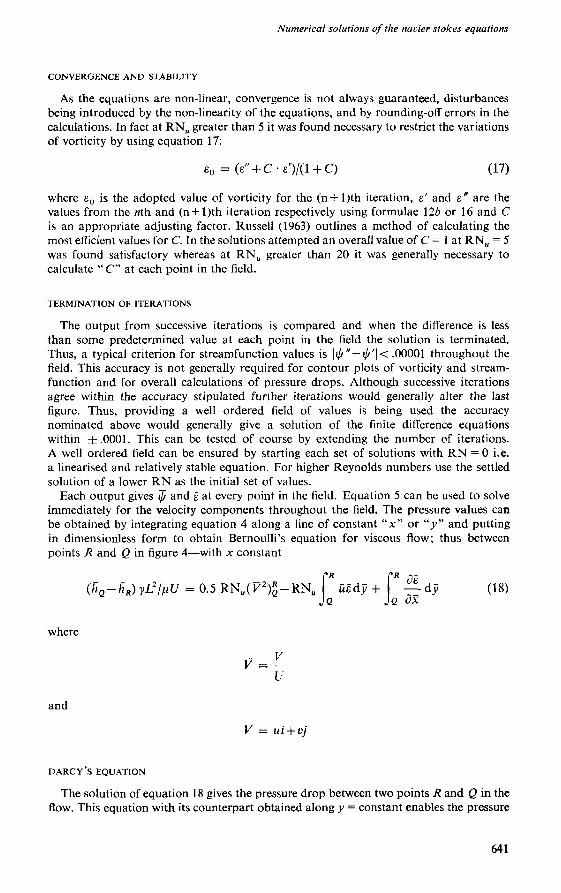
Each output gives \¡¡ and ë at every point in the field. Equation 5 can be used to solve immediately for the velocity components throughout the field. The pressure values can be obtained by integrating equation 4 along a line of constant " x " or "y" and putting in dimensionless form to obtain Bernoulli's equation for viscous flow; thus between points R and Q in figure 4—with x constant

(hQ-hR) ylljuU = 0.5 RNU(F2)«-RN„ ûèdy + R

R^-dy (18) Q OX

where

v = v-L

and

V = ui + vj

D A R C Y ' S E Q U A T I O N

The solution of equation 18 gives the pressure drop between two points R and Q in the flow. This equation with its counterpart obtained along y = constant enables the pressure

641

K.P. S

tark

1

l.n i n

i

n

J

* n

in

•;.n

Un

1 n

*.n un

5 n

1

O

_l

CL

.

LJ

•—l

-J

cr U

J

Q£

I—

LO

-^A

^-

642

Numerical solutions of the navier stokes equations

at any point in the field to be calculated. A s the right hand side of 18 is a function of R N „ and the particular boundary configuration chosen, if these two factors are held constant

(RQ — hR)yU/nU = constant

and

U = yL2kliln (19)

where kl is a constant and /is the negative piezometric head gradient. A s Uis related to q, the seepage velocity, by a simple constant factor depending on the particle arrangement it follows that:

q = ki = -/cgradfc (20)

This is, of course, Darcy's L a w and "k" is a constant for a particular medium, fluid and R N . This proof illustrates the macroscopic basis of the law as originally defined by Darcy. In practice Darcy's L a w is assumed valid for creeping flows i.e. RN===0. For other flows both the permeability (k) and the Kozeny constant (K) must be functions of R N . Thus if permeability measurements are taken in the laboratory it is important that the range of Reynolds numbers tested agrees with the field values.

D I S C U S S I O N O F R E S U L T S

Approximately 60 solutions with porosities ranging from .36 to .97 and for R N „ values ranging from 0 to 100 (but generally less than 25) have been obtained. A few interesting features of the solutions are outlined below.

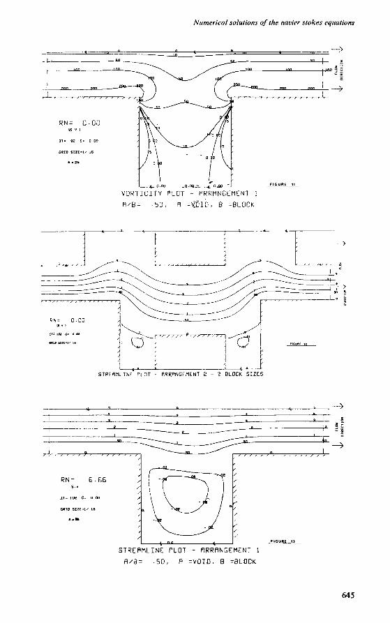
STREAMLINE AND VORTICITY CONTOURS

Figures 6 to 15, illustrate some typical streamline and vorticity contours plotted from the solutions. The manner in which the non-linear terms cause the flow pattern to become unsymmetrical at high flows is evident and the formation of the wake bubble behind each block even at zero Reynolds number is clearly illustrated. These wake bubbles are parti­cularly important in analyses of stability and fluidization of porous beds. It should be noted that the vorticity values become negative as required by the reverse flow in the wake.

VALIDITY OF DARCY'S EQUATION FOR CREEPING FLOWS

If k0 is the permeability at zero Reynolds number then the ratio of k0/k for other flows is a measure of the accuracy of Darcy's L a w for such flows. Table I gives this ratio for different flows for the m e d i u m of figure 1 with a = b i.e. porosity .75.

The usual assumption that Darcy's L a w holds for R N S 0 from 0 to 1 appears to be acceptable within the normal limits of accuracy, however, as the porosity increases or as the number of block sizes increases (see table II) the error at any particular Reynolds number also appears to increase.

PARALLEL PLATE ANALOGUE

At low flows in rock jointed masses it is usually assumed (Wittke 1966, S n o w 1965) that the flow is analogous to flow between two parallel flat plates. A n exact analytical solution is available for this analogous flow. The streamline plots indicate that, for the

643

K. P. Stark

VORTICITY PLOT

PROC NO 5J RN = 15-00

ÍS.V i

PR0CRHnnE?/-7C

i-b

-> ^ - > > * > > > > , 9 *

RN = 0.-00 IS v )

CSIO SII£=lr 16

• > I b

• xc

-*—

1 CJ fi

0 S _ ^ >

-4

/ o-c '

•

o o

ri c u m «

; , . ',

STREAMLINE PLOT - ARRANGEMENT l

R/B= -50, R =V0ID, B =BL0CK

644

Numerical solutions of the navier stokes equations

n.nn c n.nn

VDRTICITY PLOT - ARRANGEMENT 1

fl'B= -5D, fl =VfilD, B =BL0CK

STREAMLINE PLOT - ARRANGEMENT 2 - ? BLOCK SIZES

RN= G -6G

IT = 102 C= O 00

caro siit=i/ is

FIGURE 11

STREAMLINE PLOT - ARRANGEMENT 1

fVB = -50, fl =VOID. B =BLOCK

645

K.P. Stark

4a- ï

_ E Q D 2 Q Q _

• V S s / ' S / / r rç

RN = 6-BB

(S V.)

JT= ID? C = O D D

CRIO S I Z E M ' IS

VDRTICITY PLOT - ARRANGEMENT 1

A/B= -50, A :=VOIO, B -BLOCK

STREAMLINE PLOT - ARRANGEMENT d - 2 BLOCK SIZES

media analysed, as R N increases the flow pattern approaches parallel flow (e.g. figures 7 and 8). The pressure loss would naturally be less than the corresponding loss between flat plates with a spacing of b as the shear resistance along the fluid-solid interface occurs over a shorter length. This effect is counteracted to some extent by the wake flow and the inertia components. Thus, if ;' is the piezometric head gradient for a particular pattern and ip is the corresponding gradient for flow between two parallel plates at a spacing of " ¿ " then table III summarises some typical ratios of i/ip. It is seen that as the porosity decreases i.e. a> > b or as R N increases the parallel plate analogy becomes more accurate and that this analogue is m u c h less satisfactory for the arrangement of figure 2 with two block sizes than for figure 1. In rock jointed masses a/b would generally be m u c h greater than 4 . F r o m table I it is seen that k0/k is approximately constant for R N „ = 20 to 100. For these flows the streamline pattern remains very similar to parallel flow and inertia effects become rather small. These patterns are, of course, a function of the particular med ium.

646

Numerical solutions of the navier stokes equations

TABLE I

a/b (in fig.l) » 1

Porosity n «.75

RN

RN u

0. 0.01 0.05 0.10 0.50 1.0 2.0 3.0 5.0 10.0 20.0 30.0 40.0 50.0 100.0*

• RN .5

V

1.00 1.00 1.00 1.00 1.01 1.01 1.03 1.05 1.08 1.11 1.14 1.15 1.15 1.15 I.IS

* This solution was not settled completely.

TABLE II

Arrangement of Fig. 1

ratio a/b A porosity n. .36

V * at

1

2

.56

1

1

.75

RNU « 1 1.004L.00S1.01

RNU » 10 1.04 L.07 1.11

1

2/3

.84

1

1/2

.B9

1

2/5

.92

k /k values

1.02

1.13

1.02

1.16

1.02

1.16

TABLE III

Pattern

Piqûre a/b Porosity

1 4 36

1 2 SS

1 1 75

2 1 56

Values of i/ip

RNu-0 RNu-l RNu-5

.91 .92 .93

.85 .86 .89

.78 .79 .84

.48 .49 .54

1

1/3

.94

1.04

1.17

1

1/4

.96

1.05

1.30

1

1/5

.97

1.06

1.33

RN -10 u

.95

.91

.87

.61

2

1

.56

1.03

1.13

NON-LINEAR EQUATIONS - FORCHHEIMER RELATION

W h e n considering non-linear flows, as in coarse aquifers, the appropriate values of "a" and "¿>" in the Forchheimer relation are required. For a particular medium the right hand side of 18 is a function of R N thus:

(RQ-FiR)yL2lfiU = / ( R N )

and by comparison with the Forchheimer relation (3):

/(RN) = a + jS-RN

(21)

(22)

where a and ft are dependent on the medium and fluid. W h e n R N = 0, / ( R N ) 0 = a and for other values of R N

/(RN)o « k (23)

Thus by evaluating a from the numerical solution for zero R N and /? from the non-zero solutions tha appropriate values of a and b in the Forchheimer relation can be determined. The solutions show that /? is not a constant for a particular medium and fluid. However, for a given range of R N e.g. R N „ 0 to 10 one value of /? can be selected to fit the range of solutions to within 1%.

CARMAN-KOZENY (K) - POROSITY FACTOR

The solutions obtained for creeping flows can be directly compared with experimental results reported by Lord (1955) and analytical results reported by Happel and Brenner (1965) for flow in two dimensional media. The experimental results were carried out on wool, cotton and other fibres by Lord whereas Happel and Brenner analysed the linearised Stokes equation for flow at right angles to an idealised array of circular cylinders by assuming each representative particle was enclosed within a frictionless "free-surface" cell.

647

K. P. Stark

Figure 16 compares these solutions with the zero R N solutions for figure 1 by plotting Kozeny K against porosity.

P O R O S I T Y v K Q 2 E N Y K

cross hatched Lord

45 —• »—— figure 1

40

—• • Happel,Brenner

35

F I G U R E 16.

It will be noted that the results for the two idealised arrays do not differ greatly from the experimentally determined results for randomly arranged fibres of remarkably different shapes. The difference between the curves is very likely attributable to the inadequacy of the shape factor term in the C-K relation. It would appear, however, to be approximately correct. O n the other hand the porosity term is obviously inadequate as indicated by the wide range of K with porosity. A great variety of porosity factors exists in the literature, however, m a n y of the determinations have relied on an inadequate range of porosities or on a variety of particle shapes coupled with a wide range of porosities. A n appropriate porosity factor determined from the numerical solutions which gives an approximately constant value of K for the results of Lord and Happel and Brenner is n3/(l -ri)1.5. This modified value of K (called K0) will be related to the conventional value of equation 2 by

À - 0 = K - ( l - n ) ° - s (24)

D R A G COEFFICIENTS A N D STRESS DISTRIBUTIONS

The stress distribution around a typical particle in the medium can be found by calculating the pressures, as already outlined, and the normal and tangentical viscous components (Stark, Volker, 1967). These stress distributions around the particle allow the drag to be calculated. A comparison has been m a d e of the drag coefficients calculated from the results of table I with the experimental values reported by G u n n and Malik (1966) for flow through a cubic arrangement of spheres with a spacing between sphere centres of

648

Numerical solutions of the navier stokes equations

1.5 diameters normal to the flow and 1.0 diameter parallel to the flow (n = .767). The coefficients for R N S U = 0 to 100 compare favourably altough the particle shapes vary considerably. Similar agreement has been found w h e n the analytical resuls outlined are compared with results obtained numerically for flow past circular cylinders.

CONCLUSIONS

The numerical solutions outlined give encouraging results when applied to an idealised medium. These results appear to have substantial agreement with experimentally determined data and provide a very satisfactory method of investigating the basic laws and the fundamental parameters of porous media flow. A n extension of these techniques to three dimensional problems is possible with present day computer facilities.

ACKNOWLEDGEMENT

T h e author expresses gratitude to Professor D . H . Trollope for encouragement o n this project and to the W a t e r Research Foundation of Australia for financial assistance.

REFERENCES

1. A R A V I N , V . I . and N U M E R O V , S . N . (1965): «Theory of fluid flow in undeformable porous media. " Israel Prog. Scient. Trans., Jerusalem.

2. C A R M A N , P . C . (1937): Trans. Inst. Chem. Engrs., 15, 150. 3. E N G E L U N D , F . (1953): Hydraulics Labs. Bull., N o . 4 . , Tech. Univ. of Denmark . 4. F O R C H H E I M E R , P . H . (1901): "Wasserbewegung durch Boden " Zeitschrift Verein Deut. Ing., 49. 5. F R O M M , J .E. (1963): Los Alamos Scient. Lab. Report LA-2910 . 6. G U N N , D . J . and M A L I K , A . A . (1966): Trans. Instn. Chem. Engrs., Vol. 44, T 371. 7. H A M I L I E C , A . E . et al. (1967): A.I.Ch.E. Jnl., March 1967, P212. 8. H A P P E L , J. and B R E N N E R , H . (1965): Low Reynolds number hydrodynamics, Prentice Hall,

Inc. Englewood Cliffs, N . J . 9. H A R L O W , E . H . (1964):Methods in Computational Physics, Vol. 3, Academic Press N . Y .

10. K A W A G U T I , M . (1953): Rep. Inst. Soc. Japan 8 (6), 747-57. 11. K O C H I N A - P O L U B A R I N O V A , P . Y a . (1962): Theory of Ground water movement, Princeton Univ.

Press. 12. Li, W . H . and L A M , S. H . (1964): Principles of Fluid Mechanics, Addison Wesley. 13. L I N D Q U I S T , E . (1933): Rep. to 1st Congress on Large Dams, Stockholm. 14. L O R D , E . (1955): Textile Inst. Manchester Jri, Vol. 46, T191. 15. M U S K A T , M . (1946): The flow of homogeneous fluids through porous media, J. W . Edwards Inc.

A n n Arbor, Mich. 16. P H I I L P , J .R. (1957): 2nd Aust. Conf. of Soil Science, Vol. 1. 17. R U S S E L L , D . B . (1963): Aeron. Res. CouncilR. and M . , N o . 3331, H . M . S . O . 18. S C H E I D E G G E R , A . E . (1960): The physics of flow through porous media, Macmillan C o . N . Y . 19. S C H L I C H T I N G , R . (I960): Boundary Layer Theory, M c G r a w Hill. 20. S N O W , D . T . (1965): Dissertation P h . D . degree in Eng. Science, Univ. of Calif., Berkeley. 21. S T A R K and V O L K E R (1967): Res. Bull., N o . 1, April 1967, Univ. College of Townsville. 22. T E K , M . R . (1957): Trans., A.I.M.M.E., Vol. 210, p. 376. 23. T H O M , A . (1928): Aeron. Res Council R and M . N o . 1194 H . M . S . O . 24. T H O M , A . and A P E L T C . S . (1961): Field Computations in engineering and physics, Nostrand C o .

Ltd. 25. W A T S O N , K . K . (1963): Proc. 4th Aust.-N.Z. Conf. on Soil Mech. and Found. Eng. 26. W I T T K E , W . (1966): Proc. 1st Congress Inst. Soc. Rock. Mech., Lisb. 27. W O O D S , L . C . (1954): Aeronautical Quarterly, Vol. 2 pp. 176-84.

649