NUREG/CR-6786 ANL-01/30

ANL/CANTIA: A Computer Code for Steam Generator Integrity Assessments

Argonne National Laboratory

U.S. Nuclear Regulatory Commission Office of Nuclear Regulatory Research Washington, DC 20555-0001

AVAILABILITY OF REFERENCE MATERIALS IN NRC PUBLICATIONS

NRC Reference Material

As of November 1999, you may electronically access NUREG-series publications and other NRC records at NRC's Public Electronic Reading Room at http Ilwww nrc cqov/reading-rm html. Publicly released records include, to name a few, NUREG-series publications; Federal Register notices; applicant, licensee, and vendor documents and correspondence; NRC correspondence and internal memoranda; bulletins and information notices; inspection and investigative reports; licensee event reports; and Commission papers and their attachments.

NRC publications in the NUREG series, NRC regulations, and T/tle 10, Energy, in the Code of Federal Regulations may also be purchased from one of these two sources. 1. The Superintendent of Documents

U.S. Government Printing Office Mail Stop SSOP Washington, DC 20402-0001 Internet: bookstore.gpo.gov Telephone: 202-512-1800 Fax: 202-512-2250

2. The National Technical Information Service Springfield, VA 22161-0002 www.ntis.gov 1-800-553-6847 or, locally, 703-605-6000

A single copy of each NRC draft report for comment is available free, to the extent of supply, upon written request as follows: Address: Office of the Chief Information Officer,

Reproduction and Distribution Services Section

U.S. Nuclear Regulatory Commission Washington, DC 20555-0001

E-mail: DISTRIBUTION@nrc.gov Facsimile: 301-415-2289

Some publications in the NUREG series that are posted at NRC's Web site address http//www nrc Qov/readina-rm/doc-collections/nur.nsare updated periodically and may differ from the last printed version. Although references to material found on a Web site bear the date the material was accessed, the material available on the date cited may subsequently be removed from the site.

Non-NRC Reference Material

Documents available from public and special technical libraries include all open literature items, such as books, journal articles, and transactions, Federal Register notices, Federal and State legislation, and congressional reports. Such documents as theses, dissertations, foreign reports and translations, and nonNRC conference proceedings may be purchased from their sponsoring organization.

Copies of industry codes and standards used in a substantive manner in the NRC regulatory process are maintained at

The NRC Technical Library Two White Flint North 11545 Rockville Pike Rockville, MD 20852-2738

These standards are available in the library for reference use by the public. Codes and standards are usually copyrighted and may be purchased from the originating organization or, if they are American National Standards, from

American National Standards Institute 11 West 4 2 nd Street New York, NY 10036-8002 www.ansi.org 212-642-4900

Legally binding regulatory requirements are stated only in laws; NRC regulations; licenses, including technical specifications; or orders, not in NUREG-series publications. The views expressed in contractor-prepared publications in this series are not necessarily those of the NRC.

The NUREG series comprises (1) technical and administrative reports and books prepared by the staff (NUREG-XXXX) or agency contractors (NUREG/CR-XXXX), (2) proceedings of conferences (NUREG/CP-XXXX), (3) reports resulting from international agreements (NUREG/IA-XXXX), (4) brochures (NUREG/BR-XXXX), and (5) compilations of legal decisions and orders of the Commission and Atomic and Safety Licensing Boards and of Directors' decisions under Section 2.206 of NRC's regulations (NUREG-0750).

DISCLAIMER: This publication was prepared with the support of the U.S. Nuclear Regulatory Commission (NRC) Grant Program. This program supports basic, advanced, and developmental scientific research for a public purpose in areas related to nuclear safety. The grantee bears prime responsibility for the conduct of the research and exercises judgement and original thought toward attaining the scientific goals. The opinions, findings, conclusions, and recommendations expressed herein are therefore those of the authors and do not necessarily reflect the views of the NRC.

I

• , m ...................... "l'"

NUREG/CR-6786 ANL-01/30

ANL/CANTIA: A Computer Code for Steam Generator Integrity Assessments

Manuscript Completed: December 2001 Date Published: September 2002

Prepared by S. Majumdar

Argonne National Laboratory 9700 South Cass Avenue Argonne, IL 60439

J. Davis, NRC Project Manager

Prepared for Division of Engineering Technology Office of Nuclear Regulatory Research U.S. Nuclear Regulatory Commission Washington, DC 20555-0001 NRC Job Code W6487

I

ANLJCANTIA: A Computer Code for Steam Generator Integrity Assessments

by

Saurin Majumdar

Abstract

This report summarizes the work carried out to modify and expand the capability of the steam generator integrity code CANTIA originally developed for CANDU reactors. The basic algorithms for the Monte Carlo simulation, the random initiation of cracks, the effect of inservice inspection including the probability of detection (POD) of cracks, and the inclusion of plugging criteria for defective tubes have been retained. Additional ligament rupture, unstable burst, and leak rate models for Alloy 600 tubes that have been developed or validated at Argonne National Laboratory have been incorporated into the code. Fracture mechanics models for crack growth rate based on stress corrosion cracking data from the literature have also been added. The basic treatment of flaw growth has been changed from one- to two-dimensional, and crack growth calculations have been made more rigorous.

Hii

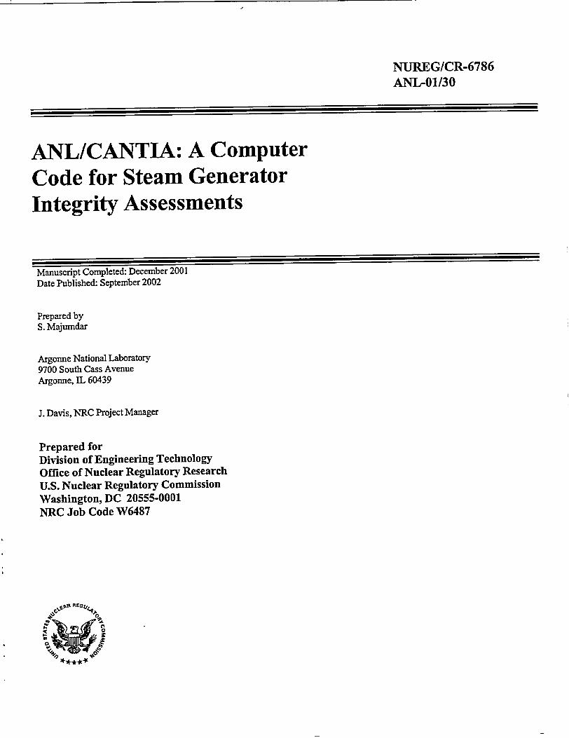
Contents

Executive Sum m ary ................................................................................................................. xI

Acknowledgm ents .................................................................................................................... xii

List of Acronym s ...................................................................................................................... xm..

List of Symbols ......................................................................................................................... xiv

1 I Introduction .................................................................................................................... 1

2 Description of CANTIA .................................................................................................... 2

2.1 Description of Input Data for CANTIA .................................................................. 3

2.1.1 General Data ............................................................................................. 3

2.1.2 Initial Flaw Size Distribution .................................................................... 4

2.1.3 Flaw Size Dim ensions ............................................................................... 6

2.1.4 Number of Flaws and Number of Tubes in Inspection Sample ............... 7

2.1.5 Eddy Current Inspection Param eters ........................................................ 7

2.1.6 Flaw Growth Distribution ......................................................................... 9

2.1.7 Flaw Initiation Distribution ....................................................................... 11

2.1.8 Tube Failure M odels .................................................................................. 11

2.1.9 Leak Rate M odel ......................................................................................... 12

2.1.10 M axim um Allowable Leak Rate ................................................................. 13

2.1.11 M aterial and Tube Dim ensional Properties ............................................... 13

2.1.12 Future Inspection Plans ............................................................................. 13

3 Features Added to CANTIA (ANL/CANTIA) ..................................................................... 15

3.1 Initial Flaw Size Distributions ............................................................................... 15

3.2 Flaw Growth M odel ................................................................................................ 15

3.2.1 Stress Intensity Factor for Part-Throughwall Cracks ............................... 15

3.2.2 Stress Intensity Factor for Throughwall Cracks ....................................... 17

3.2.3 Stress Corrosion Crack Growth Rate ........................................................ 17

3.3 Failure M odels ........................................................................................................ 18

V

3.3.1 Axial Crack Failure M odels ........................................................................ 18

3.3.2 Circum ferential Crack Failure M odels ...................................................... 19

3.4 Leak Rate M odels ................................................................................................... 20

3.4.1 Crack Opening Area for Axial Cracks ........................................................ 21

3.4.2 Crack Opening Area for Circumferential Cracks ...................................... 21

3.5 Residual stress ....................................................................................................... 22

4 Exam ples Run with ANL/CANTIA .................................................................................. 23

4.1 Effect of POD .......................................................................................................... 25

4.2 Effect of Crack Initiation ........................................................................................ 29

5 Conclusions and Recommendations for Future Work ................................................... 32

References ................................................................................................................................ 34

vi

Figures

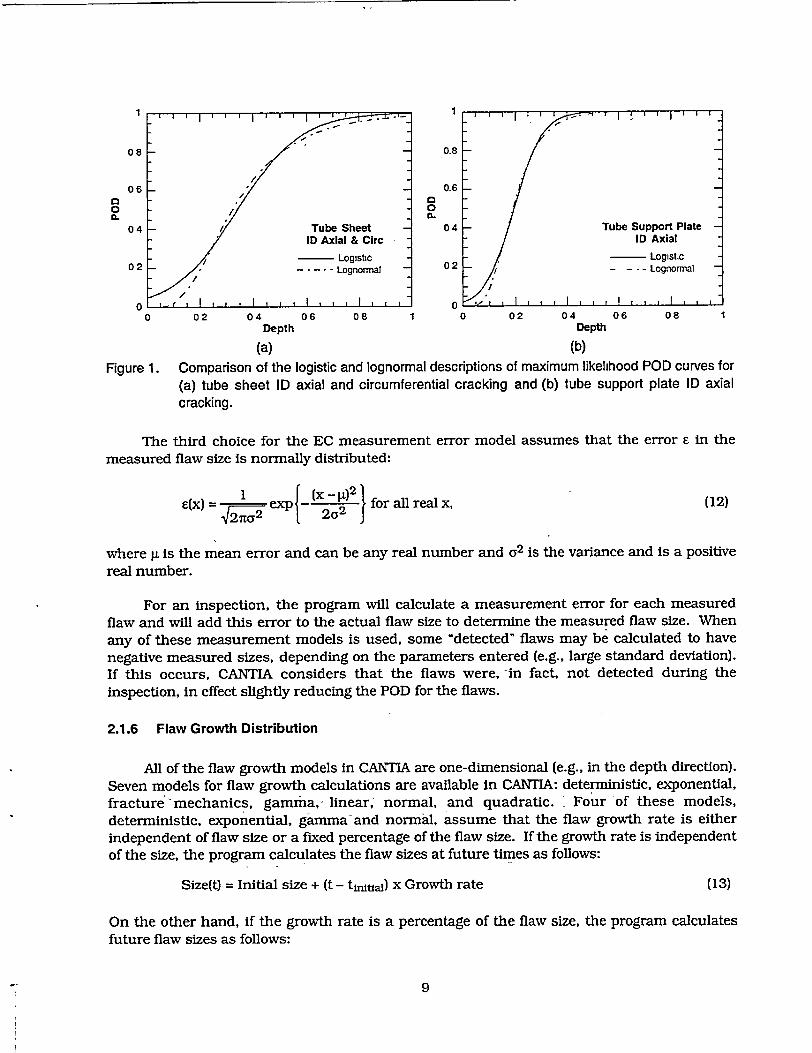
1. Comparison of the logistic and lognormal descriptions of maximum likelihood POD curves for tube sheet ID axial and circumferential cracking and tube support plate ID axial cracking ...................................................................................... 9

2. Collected literature data on crack growth rate vs. stress intensity factor for Alloy 600 in simulated primary water together with those predicted by Scott's empirical model for PWSCC and Ford and Andresen model ......................................................... 18

3. Predicted vs observed unstable burst pressures and ligament rupture pressures of Alloy 600 tubes with machined notches .................................................................... 19

4. Comparison of calculated vs. experimentally measured leak rates for as-received 22-mm (7/8 in.)-diameter tubes with 25.4 mm (1 in.) axial EDM notch at 20°C and 12.7 mm (0.5 in.) axial EDM notch at 2820 C ................................. 22

5. Variation of crack depth with time calculated deterministically for two values of initial residual stress ...................................................................................................... 23

6. Variation of the distribution of crack depth with time for initial residual stress of 30 ksi ............................................................................................................................... 24

7. Variation of the distribution of crack depth with time for initial residual stress of 40 ksi ............................................................................................................................... 24

8. Comparison of deterministically calculated crack depth with the crack depth at peak probability calculated by ANL/CANTIA for initial residual stress of 30 ksi and 40 ksi ....................................................................................................................... -24

9. Variation of the distribution of crack length with time for initial residual stresses of 30 ksi and 40 ksi ........................................................................................................ 25

10. Variation of probability of burst of one or more tubes with time for two values of initial residual stresses ................................................................................................... 25

11. Variation of probability of burst of one or more tubes with time for initial residual stress = 30 ksi for a POD = 0.9 and inspection interval of 10,000 h ............................ 26

12. Variation of the distribution of crack depth and crack length with time for initial residual stress of 30 ksi and POD = 0.9 ........................................................................ 26

13. Variation of probability of burst of one or more tubes with time for initial residual stress = 30 ksi for a POD = 0.6 and inspection interval of 10,000 h ............................ 26

14. Variation of the distribution of crack depth and crack length with time for initial residual stress of 30 ksi and POD = 0.6 ........................................................................ 27

15. Variation of probability of burst of one or more tubes with time for initial residual stress = 30 ksi for a POD = 0.01 and inspection interval of 10,000 h .......................... 27

vii

16. Variation of the distribution of crack depth and crack length with time for initial residual stress of 30 ksi and POD = 0.01 ..................................................................... 27

17. Variation of the distribution of crack depth and crack length with time for initial residual stress of 30 ksi and using POD curve for TSP ID flaws and a constant PO D = 0.6 ........................................................................................................................ 29

18. Variation of probability of rupture of one or more tubes with time for a constant POD = 0.6 and a POD curve for TSP/ID flaws and. assuming no new flaw in itiation .......................................................................................................................... 29

19. Two cases of cumulative Weibull distributions assumed for crack initiation times ..... 30

20. Evolution of the distribution for the number of flaws with time for Weibull initiation case 1 and case 2 ............................................................................................ 30

21. Distributions of crack depth calculated without initiation and with Weibuil initiation case 1 and case 2 ............................................................................................ 31

22. Distributions of crack length calculated without initiation and with Weibull initiation case 1 and case 2 at 30,000 h and 80,000 h ................................................. 31

viii

Table

1. Linear logisitic and lognormal fits to maximum likelihood POD and 95% confidence limit POD curves ....................................................................................... 8

ix

I

Executive Summary

This report summarizes work carried out to modify and expand the capability of the steam generator integrity assessment code CANTIA (CANDU Tube Inspection Assessment). CANTIA was developed by Dominion Engineering, Inc. under contract from Atomic Energy Control Board of Canada [now the Canadian Nuclear Safety Commission] to simulate the effects of tube inspection and maintenance strategies on the operation of steam generators for CANDU reactors. The integrity and leak rate models in CANTIA were specifically intended for CANDU steam generators.

Under the Nuclear Regulatory Commission sponsored Integrated Steam Generator Tube Integrity Program (ISGTIP-2), Argonne National Laboratory has developed and/or validated several models for predicting ligament rupture, unstable burst, and leak rate of flawed Alloy 600 tubes. It was decided to use CANTIA as a vehicle for incorporating these integrity and leak rate models into an integrity assessment code. Several other modifications were also made in ANL/CANTIA. The source language of the code was updated to Visual BASIC 6. The treatment of the basic flaw was changed from one-dimensional to two-dimensional and the calculation routines for crack growth were made more rigorous. Two well-known stress corrosion crack growth models from the literature were included as options, and a simple residual stress model has been added. ANL/CANTIA can handle either axial or circumferential cracks, but not both simultaneously.

Preliminary trial runs demonstrated that it is very difficult to grow stress corrosion cracks in SG tubes by pressure stress alone. Several trial runs with residual stress were conducted to demonstrate the importance of probability of detection (POD) and initiation of new cracks on rupture and leak rate probabilities.

A list of future modifications to further improve the capability of the code is included.

xi

Acknowledgments

The author thanks the Canadian Nuclear Safety Commission for providing the source code of CANTIA. Thanks are also due to Professor Jeries Abou-Hanna of Bradley University (Peoria, IL) and a student research associate, Adam Florzak who were responsible for writing the Visual BASIC code needed for the modifications. This work is sponsored by the Office of Nuclear Regulatory Research, U.S. Nuclear Regulatory Commission, under Job Code W6487; Project Manager Dr. J. Muscara.

xii

--- L-

List of Acronyms

ANL Argonne National Laboratory

BWR Boiling water reactor

CANTIA CANDU Tube Inspection Assessment

COA Crack opening area

COD Crack opening displacement

EC Eddy current

ISGTIP-2 Integrated Steam Generator Tube Integrity Program

ISI In-service inspection

NRC (U.S.) Nuclear Regulatory Commission

PNNL Pacific Northwest National Laboratory

POD Probability of detection

PWR Pressurized water reactor

PWSCC Primary water stress corrosion cracking

RT Room temperature

SCC Stress corrosion cracking

SG Steam generator

TSP Tube support plate

'AW Throughwall

xdiii

List of Symbols

A crack opening area

A, n crack growth rate constants

B constant for defining stress intensity factor

a crack depth

ac critical crack length

a, b parameters for linear-logistic distribution and flaw size measurement model

b, 0 parameters for Weibull distribution

B(al, a2) beta function

c, ce half crack and half effective crack lengths

E Young's modulus

fix) function of x

h wall thickness

K, KI stress intensity factor

K flow stress parameter

Kth threshold stress intensity factor

k, X parameters for gamma function

m bulging factor

mp ligament stress magnification factor

N, k, P parameters for negative binomial distribution

p pressure

Pburst, Pcr unstable burst pressure

p(k) probability of observing k flaws

Q leak rate

xiv

Rm, Ro. R1 mean radius (or radius of curvature), outer radius, and inner radius of

tube

S stress

Sy, Su yield and ultimate tensile strengths

T, Tf temperature and failure temperature

t, tial time and initial time

t wall thickness

t, x integration variables

a, 03 parameters for log-logistic distribution

a,, a2 parameters for beta function

Ap pressure differential

, X parameters for Gumbel distribution

8 flow stress temperature correction factor

r'(x) gamma function

a, a parameters for normal and lognormal distributions

p density of water

a stress, hoop stress

U flow stress

Glig ligament stress

Cym, b membrane and bending stresses

ay. au yield and ultimate tensile strengths

0 half circumferential crack angle

xv

1 Introduction

The Nuclear Regulatory Commission (NRC) is developing a "performance-based" regulatory framework to assure steam generator tube integrity. Instead of just meeting

prescribed rules on allowable flaw sizes for tubes that have been inspected, evaluations and

assessments are necessary to show that adequate levels of integrity can be maintained until

the next scheduled outage. The industry has developed codes and procedures to carry out

these assessments. It would be desirable to have a comprehensive validated model that

integrates all important aspects of integrity evaluations starting from in-service inspection results and ending with a total leak rate at the end of an operating cycle under various

assumed conditions. ANL/CANTIA is intended to provide a tool that could be used for

independent assessment of steam generator integrity.

Under contract from the Atomic Energy Control Board of Canada [now the Canadian

Nuclear Safety Commission], Dominion Engineering, Inc. 1 developed a Monte Carlo-based code

called CANTIA (CANDU Tube Inspection Assessment) to simulate the effects of tube inspection and maintenance strategies on the safe operation of CANDU design nuclear steam generators.

The integrity and leak rate models in CANTIA were specifically intended for the CANDU steam generators in Canada. A decision was made to use CANTIA as a framework for the development of a comprehensive integrated model of steam generator Integrity and to incorporate into CANTIA the integrity and leak rate models that have been developed at ANL under the

Integrated Steam Generator Tube Integrity Program (ISGTIP-2) sponsored by the NRC. The original CANTIA was written in Visual Basic 3.0, and a copy of the program, together with the

user's manual were obtained by ANL from the AECB. The program was updated to Visual BASIC 6.0 to run in a Windows NT environment and was then modified to incorporate the

integrity and leak rate models developed at ANL. The basic Monte Carlo simulation portion of

the code, together with much of the input format, were retained in the modified CANTIA code, renamed ANL/CANTIA.

I

2 Description of CANTIA

The CANTIA code uses Monte Carlo techniques to determine probabilities of steam generator tube failures under accident conditions and primary-to-secondary leak rates under normal and accident conditions in the future. An initial flaw size distribution is input and the program determines future flaw size distributions. The effect of inspections of the steam generator tubes at future points in time, and subsequent removal of defective tubes from the population on the probabilities of failure and leak rates and the future flaw size distributions is calculated. Thus the effect of different inspection and maintenance strategies on the probability of tube failure and primary-to-secondary leak rate can be determined.

CANTIA is designed to handle various defect types (including circumferential and axial stress corrosion cracks [SCCs], frets, and pits), though only one type of degradation can be modeled at a time. All tubes modeled in a trial are treated as being equally susceptible to the chosen degradation mode, so that the same distributions of growth rates, flaw initiation, etc., are used for all the tubes in the trial. If different distributions are believed to describe the degradation in different parts of the steam generator, then separate simulations should be run with the appropriate distributions for the portion of generator being modeled.

CANTIA uses a probabilistic failure model. It calculates a time-dependent flaw size and number distribution so that the probability of failure or the rate of leakage can be estimated. It uses a Monte Carlo approach; each important parameter is treated as a random variable with known or predictable median behavior and a known or predictable distribution of behavior (i.e., variation) around the median. Both the median and variance of each random variable are specified by the user, or, if desired, a fixed (deterministic) value can be used. For each Monte Carlo trial, the value of each variable is chosen randomly in accordance with the selected distribution function, or the fixed value is used, so that the trials reflect the variability of the actual situation. A large enough number of trials (chosen by the user) are then run for each analysis to provide a stable statistical distribution of the results.

For each Monte Carlo trial, CANTIA determines flaw sizes, growth rates, inspection results, material properties, etc. for each tube, and tracks the progression of the flaws in each tube throughout the model time period. After all trials are run, the conditions from each trial at each time of interest are compiled to determine the distributions of flaw sizes, inspection results, leak rates, and tube failures at the times of interest. The steps used in the process are as follows:

(1) All of the input parameters are checked to ensure that they are valid for the assumptions selected by the user (e.g., valid numbers are entered for the selected measurement error distribution). They are then imported into the calculational portion of the program, and the necessary arrays and variables are set up for use by the program.

(2) If the user has entered a "measured' initial flaw distribution as opposed to an "actual" one, the "actual" flaw distribution is estimated from the measured flaw distribution density f(x) by dividing f(x) by the probability of detection function POD(x) and then renormalizing. Thus the number of flaws initially present is increased to account for the undetected flaws. Before dividing by the POD, the measured distribution is shifted to account for systematic measurement errors. The "actual" flaw size distribution is then

2

renormalized so its cumulative distribution is equal to i at the maximum flaw size, and

the total number of flaws in the susceptible tube population is determined by dividing the

number of flaws present in the inspected tube sample by the fraction of the susceptible

population inspected.

(3) Next, the individual trials are begun. CANTIA randomly selects a flaw size from the .actual" flaw size- distribution (whether entered by the user or calculated from the

measured flaw size distribution and POD) for each tube with a flaw at the initial time.

Initiation times for flaws in tubes without initial flaws are also randomly selected; the size

of the flaw at the time of initiation is selected by the user. Flaw growth rates are then

randomly selected for each tube in the modeled population, and the size of the flaw on

each tube at each future time of interest is calculated. For a particular flaw, the growth

rate parameters are constant for all future times of interest in the trial (i.e., the growth

rate parameters do not change during a trial). However, if a flaw size dependent growth

rate model is selected, the flaw growth rate will change in a deterministic way with time.

Any necessary tube material or tube dimensional properties are also randomly selected

for each tube at this time; they also will remain constant throughout the trial.

(4) CANTIA then determines the conditions in the steam generator at each time of interest. It

begins by calculating the primary-to-secondary leak rate through each flaw under normal

and accident conditions and assessing whether or not each flaw-would cause its tube to

fail under accident conditions at the first chronological time of interest (as input by the

user). Next, inspections are performed if either the time of interest is a scheduled

inspection time (as entered by the user), or the primary-to-secondary leak rate under

normal conditions is larger than the allowed maximum (as entered by the user).

Inspections are modeled with an initial sample size and expansion rule parameters and

POD and measurement error distributions selected by the user, and are performed until

either all of the tubes are inspected or no additional expansions of the tube sample size

are required by the inspection expansion rules. Detected flaws that are larger than the

plugging limit are then "repaired" by removing the tube from the sample population. This

process is repeated for each additional time of interest.

(5) Once the calculations of flaw size distributions, leak rates, inspection results, etc. at each

time of interest are complete, CANTIA adds the results of the trial to the Monte Carlo data

set. Additional trials are then performed. After all. the trials are completed, the

statistical-model outputs desired by the user (e.g., probability of one or more tube failure,

flaw size distribution) are calculated for each time of interest and the results are saved to

a text file (if the user desires) and the program is terminated.

2.1 Description of Input Data for CANTIA

The input data needed for running CANTIA (version 1.1) are as follows:

2.1.1 - General Data

These relate to general data needed to run the probabilistic model.

3

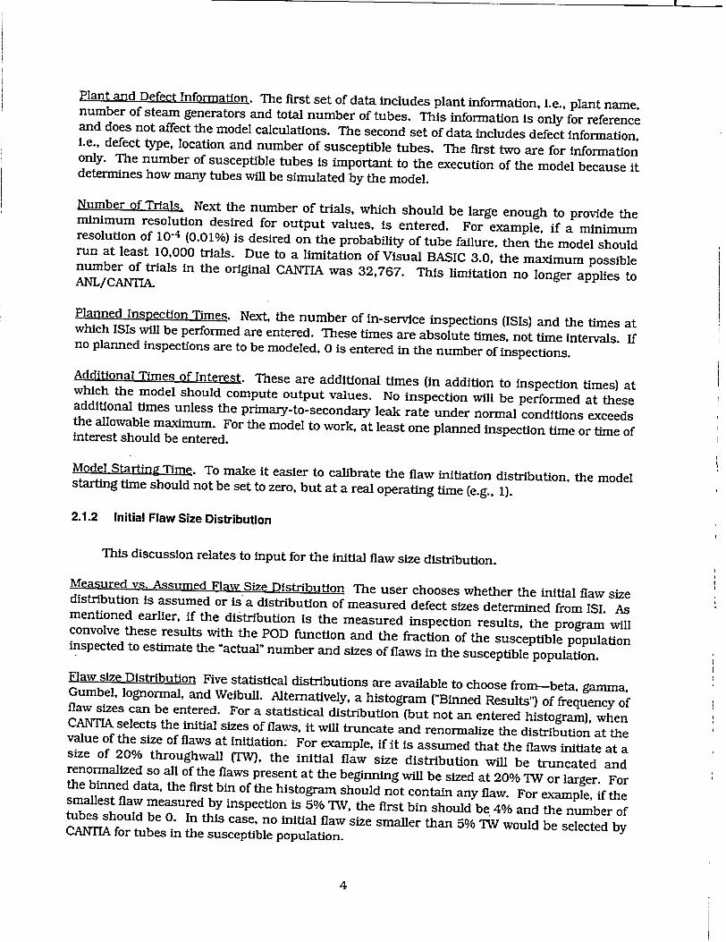
Plant and Defect Information. The first set of data includes plant information, i.e., plant name, number of steam generators and total number of tubes. This information is only for reference and does not affect the model calculations. The second set of data includes defect information, i.e., defect type, location and number of susceptible tubes. The first two are for information only. The number of susceptible tubes is important to the execution of the model because it determines how many tubes will be simulated by the model.

Number of Trials. Next the number of trials, which should be large enough to provide the minimum resolution desired for output values, is entered. For example, if a minimum resolution of 10-4 (0.01%) is desired on the probability of tube failure, then the model should run at least 10,000 trials. Due to a limitation of Visual BASIC 3.0, the maximum possible number of trials in the original CANTIA was 32,767. This limitation no longer applies to ANL/CANTIA.

Planned Inspection Times. Next, the number of in-service inspections (ISIs) and the times at which ISIs will be performed are entered. These times are absolute times, not time intervals. If no planned inspections are to be modeled, 0 is entered in the number of inspections.

Additional Times of Interest. These are additional times (in addition to inspection times) at which the model should compute output values. No inspection will be performed at these additional times unless the primary-to-secondary leak rate under normal conditions exceeds the allowable maximum. For the model to work, at least one planned inspection time or time of interest should be entered.

Model Starting Time. To make it easier to calibrate the flaw initiation distribution, the model starting time should not be set to zero, but at a real operating time (e.g., 1).

2.1.2 Initial Flaw Size Distribution

This discussion relates to input for the initial flaw size distribution.

Measured vs. Assumed Flaw Size Distribution The user chooses whether the initial flaw size distribution is assumed or is a distribution of measured defect sizes determined from ISI. As mentioned earlier, if the distribution is the measured inspection results, the program will convolve these results with the POD function and the fraction of the susceptible population inspected to estimate the "actual" number and sizes of flaws in the susceptible population.

Flaw size Distribution Five statistical distributions are available to choose from-beta, gamma, Gumbel, lognormal, and Weibull. Alternatively, a histogram ("Binned Results") of frequency of flaw sizes can be entered. For a statistical distribution (but not an entered histogram), when CANTIA selects the initial sizes of flaws, it will truncate and renormalize the distribution at the value of the size of flaws at initiation. For example, if it is assumed that the flaws initiate at a size of 20% throughwaU (TW), the initial flaw size distribution will be truncated and renormalized so all of the flaws present at the beginning will be sized at 20% 'W or larger. For the binned data, the first bin of the histogram should not contain any flaw. For example, if the smallest flaw measured by inspection is 5% TW, the first bin should be 4% and the number of tubes should be 0. In this case, no initial flaw size smaller than 5% TW would be selected by CANTIA for tubes in the susceptible population.

4

The various statistical distribution functions available in CANTIA are:

Beta Distribution

The density function for the beta distribution is:

[xal -1(1 x)a2-1 0 B(a1 , a 2 ) if0<X<1,

0 otherwise

where B(al, a 2) is the beta function defined by

B(al,a 2) =J01 ta-1(l- t)a2-1dt for any real numbers aj>O and a 2 >0.

If beta distribution is selected, the user must enter the values of a, and a2. -Note that the beta distribution is only defined from 0 to 1; therefore, it can be used only for fractional throughwall depth for flaw sizes. It cannot be used for axial length or circumferential extent

Gamma Distribution

The density function for the gamma distribution is as follows:

X0.(x)k-l e-X > fxx) x>O, (2)

0o otherwise

where F(x) is the gamma function defined by

I~x) = fo tx-le-tdt for any real number x>0.

If gamma distribution is selected, the user must enter the values of X and k. Note that since the gamma function is defined for any positive value of x, it can be used for any flaw size parameter.

Gumbel Distribution

The density function for the Gumbel distribution is:

f(x8 for all real x (3)

and where X can be any real number and 8 must be a positive real number.

If the Gumbel distribution is selected, the user must enter X and 5. Note that the Gumbel distribution is defined for any real value of x, so negative flaw sizes can occur when this

distribution is chosen. However, since the flaw size distributions are truncated and

5

renormalized at the initiation size, negative values are unlikely to be returned. The user must verify that the truncated and renormalized distribution matches the actual distribution.

Lognormal Distribution

The density function for the lognormal distribution is:

f x)Itxp-n2 x>0, fRx) = exp o2a (4)

otherwise

where g can be any real number and a must be a positive real number. Note that IL and a are, respectively, the mean and standard deviation of log(x), so the mean and variance of the lognormal distribution are exp(.+ 2/2) and exp(2g+a 2)[exp(o 2)-1J, respectively.

If the lognormal distribution is selected, the user will be required to input g. and a2 . Since the lognormal distribution is defined for any positive value of x, it can be used for any flaw size parameter.

Weibull Distribution

The density function for the Weibull distribution is:

f(x) = bO-bxb-le-(Xb x> 0, (5) 0 otherwise

where b and 0 are both positive real numbers. The mean of the Weibull distribution is (0/b) (1"1/b) and the mode of the Weibull distribution is

{ b -I j 1/b if b >1

(6) ifb<l

If the Weibull distribution is selected, the user will be required to input the values of b and 0. Since the Weibull distribution is defined for any positive value of x, it can be used for any flaw size parameter.

2.1.3 Flaw Size Dimensions

The modeling of flaw size in CANTIA is generally one dimensional, which is called the primary dimension. The primary dimension can be either percent throughwall depth, fractional depth, or axial length. Some of the failure models in CANTIA (e.g., Bruce 2 circumferential cracking model) requires a secondary dimension, which in the case of a circumferential crack would be circular arc length.

6

-1

2.1.4 Number of Flaws and Number of Tubes in Inspection Sample

For measured flaw sizes, the user must enter the number of tubes in the inspection

sample and the number of flaws found. As noted previously, the program then calculates the

actual number of flaws in the susceptible population by dividing the number of flaws found in

the inspection by the POD(x) and the fraction of susceptible tubes inspected and renormalizing.

CANTIA assumes that there is only one flaw present per tube. If the flaw size distribution is

assumed rather than from an inspection, the assumed initial number of tubes with flaws is

either a fixed number or chosen from a negative binomial distribution. The negative binomial

distribution is chosen as representative of populations where failure is not random, i.e., that certain groups in the population are more prone to failure.

Use of a negative binomial distribution allows the initial number of tubes with flaws to

vary during each trial. A negative binomial distribution with parameters N and P assumes that

the probability of observing k flaws in a steam generator is

(N + k - )(p •k, p

p(k)(N-1 +J(P~l (PJNI (7)

and the mean number of observed flaws is NP. If the negative binomial distribution is selected for the initial number of tubes in the susceptible population with flaws, N must be input as a

positive integer and P must input as a positive real number.

Because CANTIA attempts to calculate the actual number of flaws by dividing the number of detected flaws by the POD and -the fraction of susceptible tubes,' the calculation can

sometimes result in an 'actual"number of flaws greater than the-number of tubes in the

susceptible population. In such cases CANTIA will assume that all of the tubes contain a flaw and the number of susceptible tubes is unchanged. Although this may suggest an unrealistic

POD model or unrealistic inspection sample size, no explicit warning is given. To ensure that such a situation does not occur, it is best to require a printout of distribution of actual defect

size at the starting time and to verify that all of the tubes in the susceptible population do not

contain a flaw at the starting time.

2.1.5 Eddy Current Inspection Parameters

CANTIA accepts parameters that describe the POD and measurement error of the EC inspection techniques.

Probability of Detection There are three choices for POD distribution'in CANTIA: deterministic,

log-logistic, and cumulative lognormal. The deterministic POD is a fixed value of POD for all flaw depths. The log-logistic distribution is of the following form:

POD(x)= exp{x + 13 In(x)} x>O (8)

I + exp{a + 1ln(x)}

The cumulative lognormal probability function is of the form:

7

POD(x) =[1 + er hi ~xJ- (9

where g and a are the mean and standard deviation of In(x). The probability of detection (POD) curves developed from the results of the round robin tests on the ANL mockup facility have been described in terms of the linear logistic function:

POD = I. (10) 1 + ea+bx

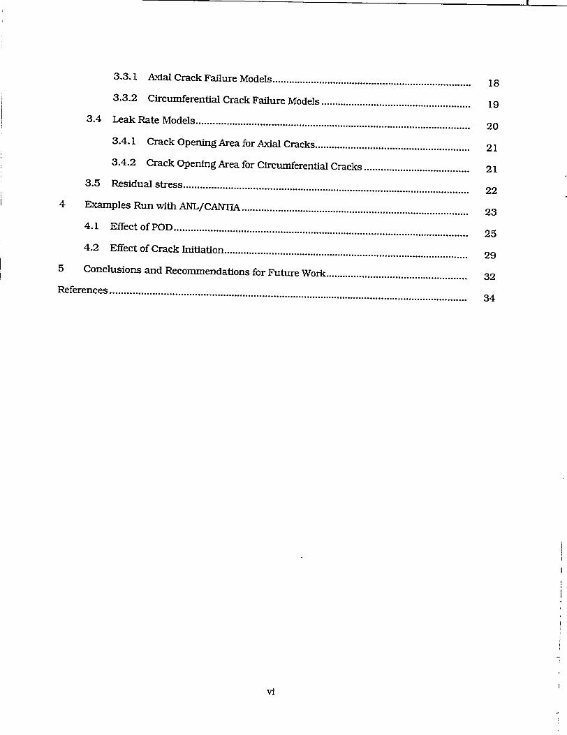
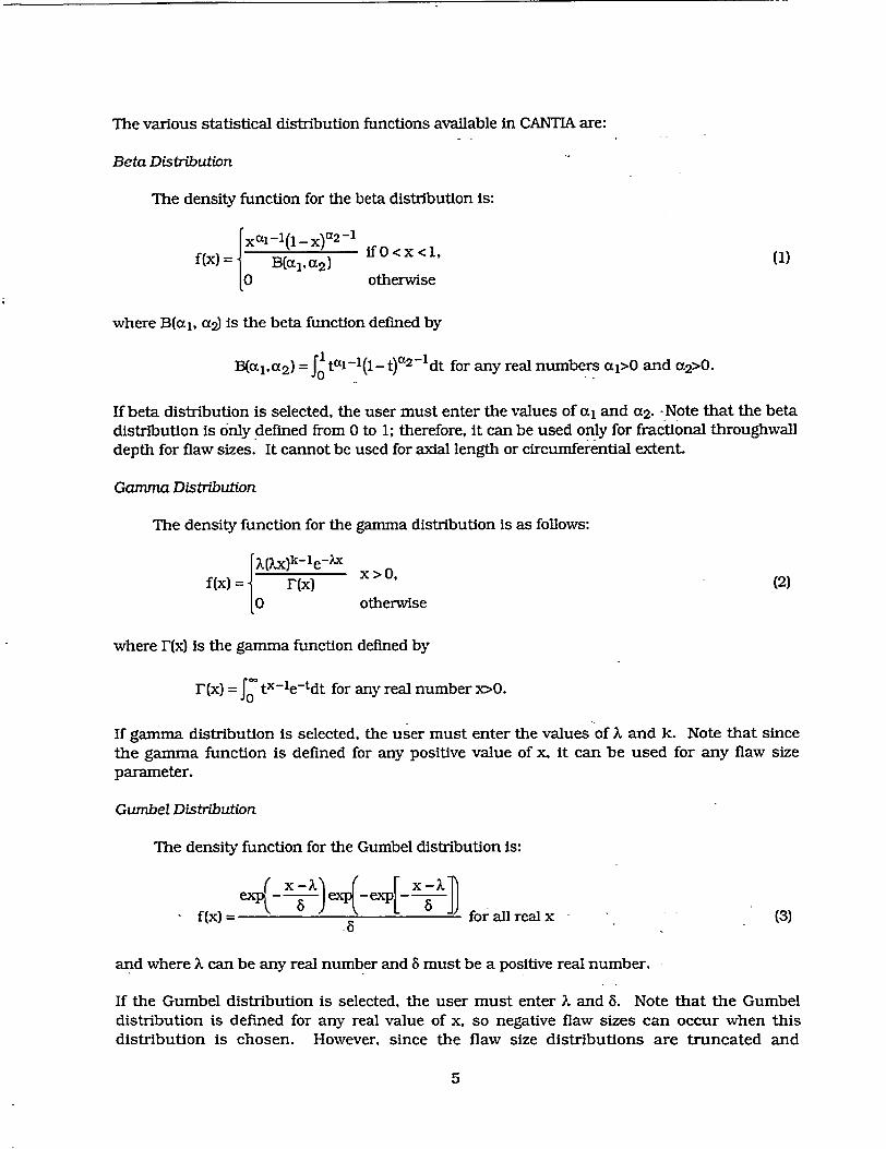
The log logistic function has a behavior quite different from the linear logistic function, but the lognormal function can provide a good approximation to the linear logistic curves with an appropriate choice of the parameters g and a. The POD curves for the tube support plate (TSP) inner and outer diameter (ID and OD) cracks, free span (FS) outer diameter cracks, and tube sheet inner diameter cracks are summarized in Table 1. Both maximum likelihood and 95th percentile one sided limits (95 OSL) are given. The root mean square errors between the linear logistic fits and the lognormal approximations range from 1.5-4.1%. Typical comparisons of the logistic and Iognormal representations of POD curves are shown in Fig. 1. Because the lognormal must vanish at 0 for all values of Ing and Ina, it cannot describe false call rates. However, in the steam generator case, these are typically fairly small, and the lognormal curves give reasonable representations of the POD curves. Table 1 Linear logisitic and lognormal fits to maximum likelihood POD and 95% confidence

limit POD curves. RMS errors in the lognormal fits are 1.5-4.1%.

Logistic POD 95 OSL Lognormal POD 95 OSL a B a b g a RMS a a RMS

TSP ID 3.96 -20.34 4.56 -20.22 -1.67 0.41 2.2 -1.52 0.36 1.6 TSP OD 3.78 -8.83 3.91 -8.16 -0.89 0.43 3.4 -0.78 0.42 3.4 FS OD 5.97 -17.17 6.74 -14.15 -1.07 0.28 1.7 -0.76 0.25 1.5 TS Axial & Circ ID 2.98 -8.69 3.58 -7.66 -1.13 0.53 4.1 -0.81 0.46 3.4

Measurement Error Model EC measurement errors can be described in CANTIA by one of three models: deterministic, linear with normal error, and normal. The deterministic model assumes that the error in the measured size is constant for all flaws. For example, if the error is -10% TW, all flaws will be sized by the EC technique as 10% smaller than their actual size. The second choice for measurement error is linear with normal error. This model assumes that the measured flaw size is a linear function of the actual flaw size with a normally distributed error or that both systematic and random errors are present in the measured flaw size distribution. The model uses the following form:

Sizemeasured = a (Sizeactuj + b + error (1I)

where a and b are constants, and the error is a normal distribution with zero mean and given variance.

8

08

06 0.6

0 0

04 Tube Sheet 04 Tube Support Plate ID Axial & Circ - ID Axial

02r- - Logistic - -- Logistic 02 Lognormal 02 Lognormal

0 9II0 *"

0 02 04 06 08 1 0 02 04 06 08 Depth Depth

(a) (b)

Figure 1. Comparison of the logistic and lognormal descriptions of maximum likelihood POD curves for

(a) tube sheet ID axial and circumferential cracking and (b) tube support plate ID axial

cracking.

The third choice for the EC measurement error model assumes that the error , in the

measured flaw size is normally distributed:

F( eXp IX-,,2 } for all real x, (12) 2i:C2• e 2a2

where gt is the mean error and can be any real number and o2 is the variance and is a positive

real number.

For an inspection, the program will calculate a measurement error for each measured

flaw and will add this error to the actual flaw size to determine the measured flaw size. When

any of these measurement models is used, some "detected" flaws may be calculated to have

negative measured sizes, depending on the parameters entered (e.g., large standard deviation).

If this occurs, CANTIA considers that the flaws were, in fact, not detected during the

inspection, in effect slightly reducing the POD for the flaws.

2.1.6 Flaw Growth Distribution

All of the flaw growth models in CANTIA are one-dimensional (e.g., in the depth direction).

Seven models for flaw growth calculations are available in CANTIA: deterministic, exponential,

fracture mechanics, gamma,- linear, normal, and quadratic. ' Four of these models,

deterministic, exponential, gamma-and normal, assume that the flaw growth rate is either

independent of flaw size or a fixed percentage of the flaw size. If the growth rate is independent

of the size, the program calculates the flaw sizes at future times as follows:

Size(t) = Initial size + (t - ttual) x Growth rate (13)

On the other hand, if the growth rate is a percentage of the flaw size, the program calculates

future flaw sizes as follows:

9

I

SGrowth Rate.•{tt-ltm~a1) Size(t) = Initial siz e(1 1 r (14) e( 100 (14

Two of the distributions used to describe flaw growth, the gamma and normal distributions, have been discussed previously [Eqs. (2) and (12)] The other two are described below:

Deterministic Model. This model assumes that the all flaws grow exactly at the same rate.

Exponential Distribution. The growth rate distribution is:

f(x) = exp > (15) 10ý otherwise"15

where jI, the mean of the distribution, is a positive real number.

The remaining three models assume the flaw growth rate is a function of the crack size:

Linear Model. The linear model for the crack growth rate is:

d(size)

dt -a size) +b, (16)

where a and b are constants, which are assumed to be normally distributed with a specified mean and variance.

Quadratic Model. The quadratic model is:

dtsize) = a(size)2 + b(size) + d, (17) d t '( 7

where a, b, and d are assumed to be normally distributed.

Fracture Mechanics Model. The fracture mechanics model is:

d~size) dt =(18)

where the stress intensity K = BSV-ie, A, B, and n are deterministic constants, and S is the nominal stress in the tube wall. The stress S is assumed to be normally distributed with a mean and variance.

If a growth rate model predicts a negative growth rate, CANTIA assumes that the flaw size is not changed.

10

2.1.7 Flaw Initiation Distribution

The flaw initiation model describes the rate over time at which new flaws initiate in the susceptible tube population. This rate is typically determined by analyzing the results of multiple inspections of the susceptible population. There are three options: no flaw initiation, lognormal distribution, and Weibull distribution. If the first option is chosen, the program will not allow any new flaws to initiate on tubes that are initially undamaged. If either the lognormal or Weibull distribution is chosen, the program will use the selected distribution to randomly select appropriate initiation times for flaws on those tubes that are undamaged at the starting time. Both lognormal and Weibull distributions have been discussed previously.

CANTIA initiates new flaws at a size defined by the user. This is the same size as is used to truncate the initial flaw size distribution.

2.1.8 Tube Failure Models

Seven failure models are available: a circumferential cracking maximum moment model, a tube burst due to fretting model, a critical flaw size model, the French tube burst due to axial primary water stress corrosion cracking (PWSCC) model, the Ontario Hydro tube burst due to axial cracking model, a tube burst due to pitting model, and the Slovene plastic collapse due to axial PWSCC model.

Because some of the models are plant-specific, their details will not be discussed here. Some of the more general failure models are as follows:

French Axial PWSCC Tube Burst Model. This model can be selected for unstable burst of isolated throughwall axial cracks away from the tubesheet and tube support plates (TSPs). The burst pressure is

Pburst mt (19)

where F is the circumferential flow stress at temperature calculated as 0.58 times the sum of yield and ultimate strengths at temperature, t is the wall thickness, Ri is the inner radius, and m is the bulging factor given by

mE 1+ Rm, (20) Rmt

where Rm is the mean radius and c is the half crack length.

Slovene Axial PWSCC Plastic Collapse Model This model was developed to determine the critical length of an axial throughwall PWSCC flaw. The critical length is the length at which the crack fails by unstable crack propagation due to net section collapse. The critical crack length, assuming an elastic Poisson's ratio of 0.3, is given by

ac =-[-.709 + 1.155m - 7.056exp(-2.966m)]-R4t, (21)

11

I

where

m K(ay + au)S mRm am q 50

K is the flow stress factor, P is the pressure differential, ay and au are the yield and ultimate strengths, respectively, and 5 is a flow stress temperature correction factor.

There is an additional equation to calculate the reinforcement effects of the tubesheet. This reinforcing factor, a correction factor for the flow stress factor K, is restricted to single cracks propagating from the tubesheet, and may not apply to multiple cracks or circumferential cracks. The reinforcement factor R1 is given by

RF(ac) = 1+ 10 (-1.8 a (22)

The program first calculates a critical half-crack length and RF for each tube based on the pressure differential during accident conditions. It then recalculates the critical half-crack length using the above two formulas for ac and m, after multiplying K by RF, and compares the length of an in-service flaw with the reinforced critical crack length to determine if the tube has failed or not.

2.1.9 Leak Rate Model

Three leak rate models were available in the original version of CANTIA: a Bruce 2 circumferential-cracking leak rate model, a model considering any "failed" tube to leak at a given rate, and a French lower-bound leak rate model for axial PWSCC. They have been retained in the present version. Because the Bruce 2 model is plant-specific, it will not be discussed here.

Fixed Leak Rate Model This model assumes that all "failed" flaws (or flaws that are 100% TW leak at the same rate (entered by the user) under either normal or accident condition.

French Lower Bound Estimate. The French equations for lower-bound leak rate are as follows:

Q = 0.3A p, (23) F p

where

A = a(-(E)--L J[(c+ ry)1 .5 - r.5], (24a)

aPX) = 1i+0. X + 0.16X2, (24b)

12

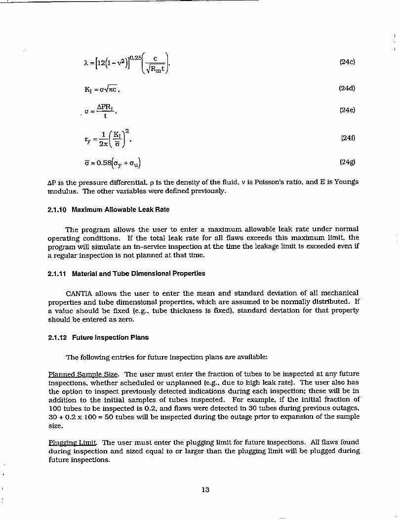
KI = a(-c, (24d)

A = AR, (24e)

t

r 1 = 1 (240

U= 0.58(oa + )(24g)

AP is the pressure differential, p is the density of the fluid, v is Poisson's ratio, and E is Youngs

modulus. The other variables were defined previously.

2.1.10 Maximum Allowable Leak Rate

The program allows the user to enter a maximum allowable leak rate under normal

operating conditions. If the total leak rate for all flaws exceeds this maximum limit, the

program will simulate an in-service inspection at the time the leakage limit is exceeded even if a regular inspection is not planned at that time.

2.1.11 Material and Tube Dimensional Properties

CANTIA allows the user to enter the mean and standard deviation of all mechanical properties and tube dimensional properties, which are assumed to be normally distributed. If

a value should be fixed (e.g., tube thickness is fixed), standard deviation for that property should be entered as zero.

2.1.12 Future Inspection Plans

The following entries for future inspection plans are available:

Planned Sample Size. The user must enter the fraction of tubes to be inspected at any future

inspections, whether scheduled or unplanned (e.g., due to high leak rate). The user also has the option to inspect previously detected indications during each inspection; these will be in addition to the initial samples of tubes inspected. For example, if the initial fraction of

100 tubes to be inspected is 0.2, and flaws were detected in 30 tubes during previous outages, 30 + 0.2 x 100 = 50 tubes will be inspected during the outage prior to expansion of the sample

size.

Plugging Limit The user must enter the plugging limit for future inspections. All flaws found

during inspection and sized equal to or larger than the plugging limit will be plugged during future inspections.

13

Sample Expansion Rule. Six expansion rules are available: two local expansion rules based on detection of a single defect larger or smaller than a given size, two global expansion rules based on detecting a fraction of flaws larger or smaller than a given size, a global expansion rule based on detecting a given number of repairable flaws, and a maximum number of expansions after which all tubes must be inspected. CANTIA cannot treat local clustering within the susceptible tubes, because tubes are assumed to be statistically independenL

When the program first simulates an inspection, after inspecting an initial sample of tubes and all tubes with previously detected flaws (if desired), it will check whether any of the expansion rules apply. It will then determine the number of additional tubes to be inspected and inpsect them. The results of additional inspections will then be checked against the selected expansion rules, and additional inspections will occur as long as any of the selected expansion rules apply, until 100% of inservice tubes are inspected, or until the maximum number of expansions (entered by user) are performed.

14 2

3 Features Added to CANTIA (ANL/CANTIA)

All of the input data structure, failure and leak rate models, and in-service inspection options available in the original CANTIA are retained in ANL/CANTIA. The basic Monte Carlo simulation algorithm was also maintained without any modification. Features that were added to CANTIA are discussed in the following sections.

3.1 Initial Flaw Size Distributions

A major feature added in ANL/CANTIA is the ability to treat the growth of twodimensional cracks, i.e., cracks are allowed to grow (by stress corrosion) both in length as well and depth. Thus, the input in ANL/CANTIA requires an initial flaw depth distribution as well as an initial flaw length distribution. Currently, the depth is taken as the primary dimension, whereas the initial length distribution is entered in terms of a distribution in the aspect ratio (length/depth). The distribution for the aspect ratio can be any of the five statistical distributions: beta, gamma, Gumbel, lognormal, and Weibull. Alternatively, a fixed deterministic ratio can be chosen.

3.2 Flaw Growth Model

The basic flaw considered in the original CANTIA is a one-dimensional flaw, e.g., an infinitell•ong shallow part-throughwall crack with a stress intensity factor K given by K = BS4size, where the user must specify constants B and S. In the ANL/CANTIA, we consider an initially elliptical two-dimensional surface flaw of length 2c and depth a. ANL/CANTIA then computes, by numerical integration (4th order Runge-Kutta), the growth (by stress corrosion) of the crack both through the wall and in length, up to the point where it becomes a throughwall crack. CANTIA then follows the growth (by stress corrosion) of the throughwall crack until unstable rupture.

3.2.1 Stress Intensity Factor for Part-Throughwall Cracks

The stress intensity factors for a part-throughwall axial or circumferential crack at its deepest point and at the surface are the solutions given by Newman and Raju 3 for a flat plate of width = 2w and thickness = t. For axial cracks, the solutions should be reasonable for shallow cracks for which bulging effects are small. For circumferential cracks, the solution should be reasonable for cases either when the tubes are constrained against bending or the cracks are short so that effects due to tube bending are negligible. The equations for the stress intensity factor KI of a part-throughwall crack in a flat plate are:

Q•K<l,-I-<O. 5,andO0:90, (25)

where 0 m and 0 b are the membrane and bending stresses, respectively, and 0 = 0-and • = 90 1 represent the surface crack tip and the crack tip at the deepest point, respectively. For axial cracks and short circumferential cracks in steam generator tubes, c/w = 0 is a good approximation. The rest of the terms are:

15

Q =1+ 1.464(aJL.

F =[Mi+ M2 (.2 + M3(.-. ]4 f g.

M, =1. 3 -0.09a

M2 = -0.54 +0.89 2-.+ a'

0.2 + C

M 3 =0-5-1. +14 1.0-a-24

0.65+ a C) C

=o [(ajCO2 0 + Si]1/ We

Pw=O'+•O6)) g =1+ [.1 + 0.3 ( _Sin

H H, + (H2 - HXsin ý)P,

p =0.2 + .ý+ 0.6()

HI =1-0.341--o.la (a), t c t)

H2 = 1 + GI(2 + G 2 ( t).

G0.55-1.205 + 0 5(.1

G2:=0.55-1.05 (0.5+ 0.47,-,1.5

16

1.

(26a)

(26b)

(26c)

(26d)

(26e)

(260

(26g)

(26h)

(260)

(26j)

(26k)

(261)

(26m)

(26n)

3.2.2 Stress Intensity Factor for Throughwall Cracks

For throughwall axial cracks, the stress intensity factor is

K, = ma-t-c (27)

where m is the bulging factor:4

m = 0.614 + 0.481X + 0.386exp(-1.25X), (28a)

and

1- 1.82c x =[12(l -v2)4~ (28b)

TRmt Tm

In the current version of ANL/CANTIA, the stress intensity factor for a throughwall circumferential crack of angular length 20 is given by

K, = OmFmn.0, (29)

where

am pR1 (30a) 2t

Fm 1+0.1501y1 5 for y ___2 Fm= t0.8875 + 0.2625y for 2 y5' (30b)

Y= FRm (30c) tM

3.2.3 Stress Corrosion Crack Growth Rate

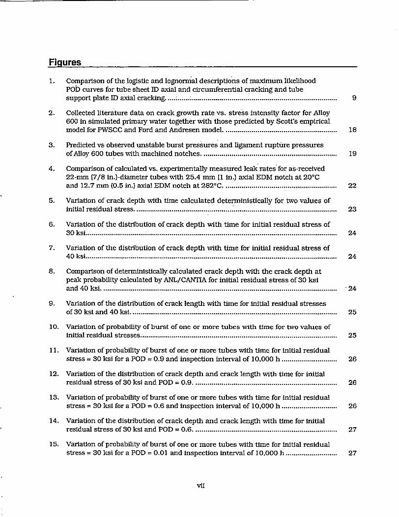
In ANL/CANTIA we have provided two models for stress corrosion crack growth rates: one due to Scott5 and the other due to Ford and Andresen. 6 It is assumed that the same equation can predict crack growth rates in the thickness and the length directions. Scott's model for PWSCC gives the crack growth rate (in urm/h) as a function of stress intensity factor (in MPa4m):

da_ 1.008 X 10-2 (KI - Kth)1-1 6 (31) dt

where Kth is a threshold stress intensity factor (typically = 9 MPa4m)

Ford and Andresen 6 developed the following equation for crack growth rate (in gm/h) as a function of stress intensity factor (in MPa;m}:

17

1

1 1 , _ Figure 2. O Ford and Andresen Collected literature data on crack model with n = 0.65 growth rate vs. stress intensity factor

0.1 ?4ý . for Alloy 600 in simulated primary water 2 E • together with those predicted by Scott's ""So1t E c empirical model for PWSCC and Ford

model foria and Andresen model. ro0.01 z•model for PWSCC

0 20 40 60 80 100 120 K,(MPa iii)

d-a =(2.808xIO n3.)(6x1O (32)

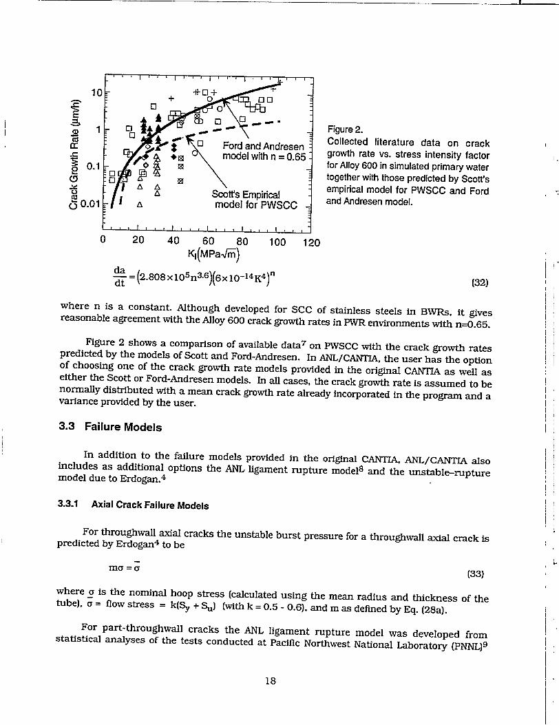
where n is a constant. Although developed for SCC of stainless steels in BWRs, it gives reasonable agreement with the Alloy 600 crack growth rates in PWR environments with n=0.65.

Figure 2 shows a comparison of available data 7 on PWSCC with the crack growth rates predicted by the models of Scott and Ford-Andresen. In ANL/CANTIA, the user has the option of choosing one of the crack growth rate models provided in the original CANTIA as well as either the Scott or Ford-Andresen models. In all cases, the crack growth rate is assumed to be normally distributed with a mean crack growth rate already incorporated in the program and a variance provided by the user.

3.3 Failure Models

In addition to the failure models provided in the original CANTIA, ANL/CANTIA also includes as additional options the ANL ligament rupture model 8 and the unstable-rupture model due to Erdogan. 4

3.3.1 Axial Crack Failure Models

For throughwall axial cracks the unstable burst pressure for a throughwall axial crack is predicted by Erdogan 4 to be

ma = a (33)

where _a is the nominal hoop stress (calculated using the mean radius and thickness of the tube), a = flow stress = k(Sy + Su) (with k = 0.5 - 0.6), and m as defined by Eq. (28a).

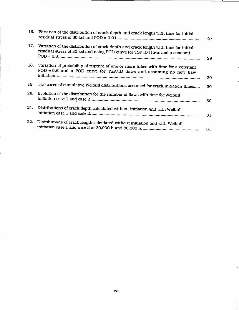
For part-throughwall cracks the ANL ligament rupture model was developed from statistical analyses of the tests conducted at Pacific Northwest National Laboratory (PNNL)9

18

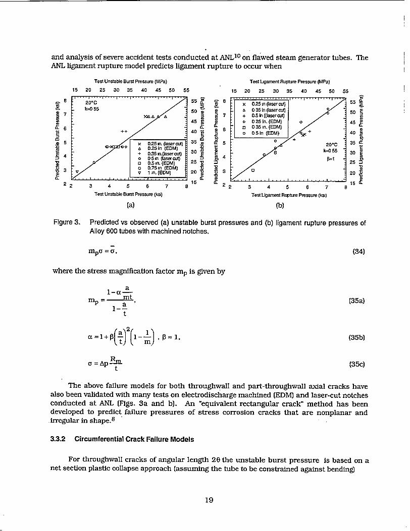
and analysis of severe accident tests conducted at ANLIo on flawed steam generator tubes. The ANL ligament rupture model predicts ligament rupture to occur when

Test Unstable Burst Pressure (MPa)

15 20 25 30 35 40 45 50 55

2 3 4 5 6

Test Unstable Burst Pressure (ksi)

(a)

7 8

Test Ligament Rupture Pressure (MPa)

15 20 25 30 35 40 45 50

55

50

45

40

35

30

25

20

15

a0

I0

S

D

8

7

6

5

CD

E 04

133

(L 2 2 3 4 5 6 7

Test Ligament Rupture Pressure (ksi)

(b)

55

8

55

50

45

40

35

30

25

20

15

S C

9D

CD E

"co tm

a,

0D

Figure 3. Predicted vs observed (a) unstable burst pressures and (b) ligament rupture pressures of Alloy 600 tubes with machined notches.

mpa =a, (34)

where the stress magnification factor mp is given by

a 1-a

mt a

t

a=l+o 1-,t=1

a = ApR t

(35a)

(35b)

(35c)

The above failure models for both throughwall and part-throughwall axial cracks have also been validated with many tests on electrodischarge machined (EDM) and laser-cut notches conducted at ANL (Figs. 3a and b). An "equivalent rectangular crack" method has been developed to predict failure pressures of stress corrosion cracks that are nonplanar and .irregular in shape.8

3.3.2 Circumferential Crack Failure Models

For throughwall cracks of angular length 20 the unstable burst pressure is based on a net section plastic collapse approach (assuming the tube to be constrained against bending)

19

7

0.6 oS 6

C5

4

V

2

ApRm (y am = - i= I-ýia (36) 2t 7Cr)

For a part-throughwall crack the ligament rupture pressure was obtained by modifying Kurihara's results for piping" 1 and is given by

-APRm

am = = -, (37) 2t In (

where

(38a)

a t

M t (38b a Nt

N=I+(X Y. (38c)

Analysis of Kurihara's data showed that X = 0.2 and y = 0.2 fitted his data to the ANL equation fairly well.8

3.4 Leak Rate Models

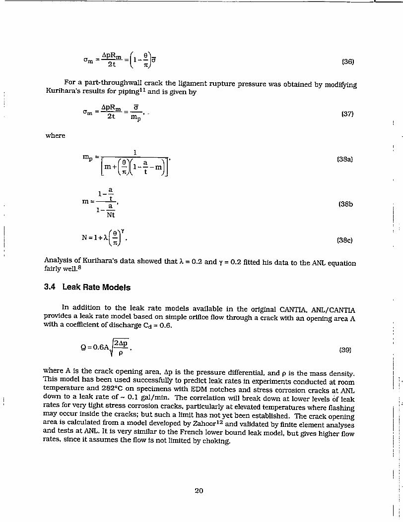
In addition to the leak rate models available in the original CANTIA, ANL/CANTIA provides a leak rate model based on simple orifice flow through a crack with an opening area A with a coefficient of discharge Cd = 0.6.

Q = 0.6A p (39)

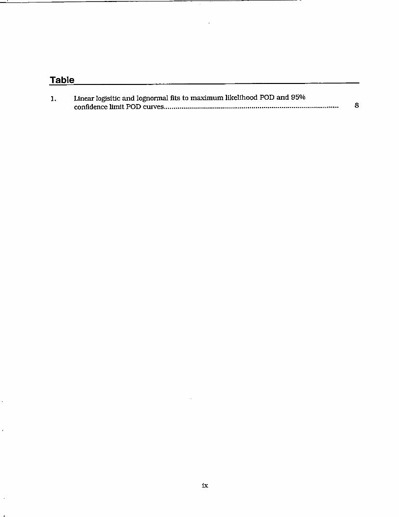
where A is the crack opening area, Ap is the pressure differential, and p is the mass density. This model has been used successfully to predict leak rates in experiments conducted at room temperature and 2820C on specimens with EDM notches and stress corrosion cracks at ANL down to a leak rate of - 0.1 gal/min. The correlation will break down at lower levels of leak rates for very tight stress corrosion cracks, particularly at elevated temperatures where flashing may occur inside the cracks; but such a limit has not yet been established. The crack opening area is calculated from a model developed by Zahoor 12 and validated by finite element analyses and tests at ANL. It is very similar to the French lower bound leak model, but gives higher flow rates, since it assumes the flow is not limited by choking.

20

3.4.1 Crack Opening Area for Axial Cracks

Zahoor's model 12 for the crack opening area A of an axial throughwall crack of length 2c

is:

A= 2ce2Vo / E, (40)

where

a = hoop stress = ApRm/t, (41a)

Ap = differential pressure across tube wall,

E = Young's modulus,

Rm and t = mean radius and thickness of tube, respectively,

V, = 1 + 0.64935X2 - 8.9683x 10-3X4 + 1.33873x 1 0 -4X6, (41b)

.e =C2/Rmt' (41c)

F =1+ 1.2987X2 -2.6905x 10- 2X4 + 5.3549x10-4X6 , (41e)

X2 =C2 / Rmt, (410)

y= yield strength.

The above approach for calculating crack opening areas and leak rates has been validated

by pressure and leak rate tests conducted at ANL on axial EDM notched specimen at room

temperature as well as at 2820C (Figs.4a-b).8

3.4.2 Crack Opening Area for Circumferential Cracks

For a throughwall circumferential crack of angular length 20, Zahoor's expression 12 for

the crack opening area is:

A2= RmtB E' (42)

where

B= 2e + 0164 e < I(43a) B=0.02 + 0.8142e + 0.3 A, + 0.03,4e Xe >1'

21

Xe =Ce F-.

Ce =0 11 F c 2

1 4 0 0 . , , I, . As-received tube

1200 25.4 mm EDM notch (20-C) 1000

"-" 0 Test E 800 x Calulated with u" 600 measured COA

C" _, 400 C4 Predicted _j 200 71,1

0 -200

-5 0 5 10 15 20Ap (MPa) (a)

60

50

-2-40

S30

S20

a10 ,-J

0

-10 -5 0 5 10 Ap (MPa)

Figure 4. Comparison of calculated (solid line) vs. experimentally measured (symbols) leak rates for as-received 22-mm (7/8 in.)-diameter tubes with (a) 25.4 mm (1 in.) axial EDM notch at 200C and (b) 12.7 mm (0.5 in.) axial EDM notch at 2820C. Cross symbols (x) in Fig. 4a denote calculated leak rates using posttest measured crack opening areas.

F= + 0.1501Io1-5 XŽ2 (43d) 10.8875 + 0.2625X X >2'

15 20

(43e)

(430

3.5 Residual stress

In ANL/CANTIA, the peak residual stress value (mean and variance) is entered by the user. Currently, the residual stress is idealized as a membrane stress that is reduced linearly with increasing crack depth until it is zero at 100% crack depth. Unless the initial crack depths are very deep, pressure stresses alone cannot grow the stress corrosion cracks through the tube wall without the assistance of residual stresses, However, the current residual stress model in ANL/CANTIA is highly simplified and should be made more realistic in the future.

22

rRm

am =Ap=-. am 2t

I

(43b)

(43c)

(b)

4 Examples Run with ANLICANTIA

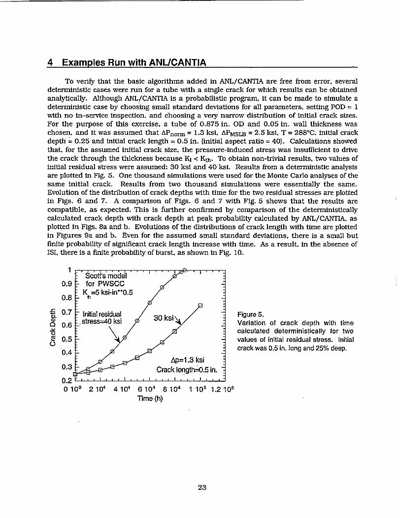
To verify that the basic algorithms added in ANL/CANTIA are free from error, several deterministic cases were run for a tube with a single crack for which results can be obtained analytically. Although ANL/CANTIA is a probabilistic program, it can be made to simulate a deterministic case by choosing small standard deviations for all parameters, setting POD = 1 with no in-service inspection, and choosing a very narrow distribution of initial crack sizes. For the purpose of this exercise, a tube of 0.875 in. OD and 0.05 in. wall thickness was chosen, and it was assumed that APnorm = 1.3 ksi, APMSLB = 2.5 ksi, T = 2880C, initial crack depth = 0.25 and initial crack length = 0.5 in. (initial aspect ratio = 40). Calculations showed that, for the assumed initial crack size, the pressure-induced stress was insufficient to drive the crack through the thickness because K, < Kth. To obtain non-trivial results, two values of initial residual stress were assumed: 30 ksi and 40 ksi. Results from a deterministic analysis are plotted in Fig. 5. One thousand simulations were used for the Monte Carlo analyses of the same initial crack. Results from two thousand simulations were essentially the same. Evolution of the distribution of crack depths with time- for the two residual stresses are plotted in Figs. 6 and 7. A comparison of Figs. 6 and 7 with Fig. 5 shows that the results are compatible, as expected. This is further confirmed by comparison of the deterministically calculated crack depth with crack depth at peak probability calculated by ANL/CANTIA, as plotted in Figs. 8a and b. Evolutions of the distributions of crack length with time are plotted in Figures 9a and b. Even for the assumed small standard deviations, there is a small but finite probability of significant crack length increase with time. As a result, in the absence of ISI, there is a finite probability of burst, as shown in Fig. 10.

1 'Scot's'r odel . .1

0.9 for PWSCC K =5 ksi-in**0.5

0.8 1h

CL 0.7 Initial residual Figure 5.

0.6 stress-4k ksi Variation of crack depth with time -~ calculated deterministically for two

S0.5 values of initial residual stress. Initial 0 crack was 0.5 in. long and 25% deep.

0.4

0.3 •Crack length=0.5 in.

0.2 , I I I

0100 2104 4104 6104 8T104 1 10( 1.210 Time (h)

23

1.2

1 t

0.8

•"0.6

0.4

0.2 il

0 0.2 0.4 0.6 0.8

Crack Depth

Figure 6. Variation of the distribution of crack depth (bin size = 0.05) with time for initial residual stress of 30 ksi.

1.2

0.2 0.4 0.6 0.8 Crack Depth

0 20000 40000 60000 80000100000120000 "Time (h)

(a)

Figure 7. Variation of the distribution of crack depth (bin size = 0.05) with time for initial residual stress of 40 ksi.

1 1.2 1.4

1.2

1

0.8

0 0.6

0.4

0.20 20000 40000 60000 80000100000120000

Time (h) (b)

Figure 8. Comparison of deterministically calculated crack depth with the crack depth at peak probability calculated by ANL/CANTIA for initial residual stress of (a) 30 ksi and (b) 40 ksi.

24

1.2

1

0.8

Z× 0.6

0.4

0.2

0

0.9

0.8

0.7

•. 0.6

S0.5

0 0.4

0.3

0.2

-e.. 10000h 30 ksi e3--20000h

0-e 30000h --X--40000h

-... 50000h - 60000h -..70000h

-i.-- 80000h1 -- *..--9000011

L *-A... 100000h

~:

05

0.4

" 0.3

02

0.1

0

0.5

04

S03

02

01

0

02 0.4 0.6 0.8 1 1.2 1.4 Crack Length (in.)

(a) Figure 9. Variation of the distribution of crack length

stresses of (a) 30 ksi and (b) 40 ksi.

0.35

0.3

= 0.25

0 0.2 202

0.15 .0

E. 0.1

0.05

0

04 06 08 1 Crack Length (in.)

(b)

12 14

(bin size = 0.05 in.) with time for initial residual

=

Figure 10. Variation of probability of burst of one or more tubes with time for two values "of initial residual stresses. Note that no ISI was assumed.

0 20000- 40000 60000 80000 100000120000 Time (h)

4.1 Effect of POD

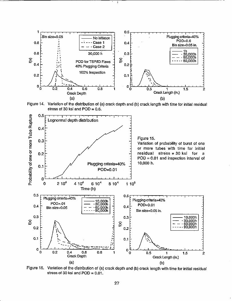
First, we evaluated the effect of fixed POD on the failure probabilities or more precisely the conditional probability of failure under a design basis accident. Evolution of the probability of one or more tube ruptures with time is plotted in Fig. 11 for the case when POD = 0.9. Variations of distributions of crack depth and crack length with time for the same POD are plotted in Figs. 12a and 12b, respectively. Similar results are plotted in Fig. 13 and Figs. 14a and b for a POD = 0.6 and in Fig.15 and Figs. 16a and b for a POD of 0.01, respectively.

25

0.606

0

0 I-

0 E 0 0, o 0

..0

0

0.5

0.4

0.2

0.1

Figure 11. Variation of probability of burst of one or more tubes with time for initial residual stress = 30 ksi for a POD = 0.9 and inspection interval of 10,000 h.

8 W0 1 1i0

0 0.2 0.4 0.6 0.8 1 0 0.5 1 1.5 2 Crack Depth Crack Length (in.)

(a) (b) Figure 12. Variation of the distribution of (a) crack depth and (b) crack length with time for initial

residual stress of 30 ksi and POD = 0.9.

0.0151

0• 0 2 1e 4 104

Time

Figure 13. Variation of probability of burst of one or more tubes with time for initial residual stress = 30 ksi for a POD = 0.6 and inspection interval of 10,000 h.

6 104 8104 1 10i

26

0 2 104 4 10 6 10 Time (h)

0

=. 0. n

.0

E 0

0) Ci

-0

..0

0 0.

- I I I I II I I ' . I i

-Bin size=0.05 _ii

-ii

- I'

- I ' I

- POD f( \, 40% Pl 100'

0.2 0.4 0.6 Crack Depth

(a)

-No initiabon --- Case 1 - -Case 2

30,000 h

r TSPPAD Flaws ugging Criteria

VoInspection

0.8 1 1 Crack Length (in.)

2

(b)Figure 14. Variation of the distribution of (a) crack depth and (b) crack length with time for initial residual

stress of 30 ksi and POD = 0.6.

2 10 410 6 104 8104

Time (h)

Figure 15. Variation of probability of burst of one or more tubes- with time for initial residual stress = 30 ksi for a POD = 0.01 and inspection interval of 10,000 h.

1 105

0 0.2 0.4 0.6 Crack Depth

0.5

0.4

0.3

0.2

0 .8 1 0.1

0.8 1 00 0.5 1 Crack Length (in.)

1.5 2

(a) (b) Figure 16. Variation of the distribution of (a) crack depth and (b) crack length with time for initial residual

stress of 30 ksi and POD = 0.01.

27

1

0.8

0.6

x 0.4

0.2

0o

W

C.

0

:0

I

0

0

2

a 50 0

..5

.CU

D. 0L 0

0.5

0.4

0.3

0.2

0.1

0

Plugging criteria--40% POD=0.01

Bin size=0.05 in.

10,000h 30,000h 60,000h 90,000h

S. . . . . . . . I • I I I I I

As expected, the probability of one or more tube rupture increases with decreasing POD. Peaks and valleys in Fig. 13 represent the effect of plugging on the probability of tube rupture. The probability of tube rupture is very small for POD = 0.9. For POD = 0.6, the probability of one or more tube rupture peaks at an intermediate time. In the case of POD = 0.01, the probability of one or more tube rupture increases monotohicallk with time. The locations of the peak in the probability of crack depth and crack length change very little with time or POD. The spikes in the probability of crack length at zero crack length represent plugged tubes. Similarly, the spike in the probability at a crack depth of 100% in Fig. 16a represent cracks that become throughwall. As expected, the probability for plugging is essentially zero when the POD = 0.01.

Next, we explored the difference between assuming a fixed probability of crack detection (POD = 0.6) and assuming a POD curve determined for TSP/ID flaws in the recent ANL mockup round robin on the probability of one or more tube rupture. Although the ANL round robin POD was best-fitted with a linear logistic curve (not available as an option in the current ANL/CANTIA), a good approximation to the POD curve can also be obtained with a lognormal curve (Fig. 1), which is one of the options in ANL/CANTIA. This lognormal curve for POD was used in the calculations and 100% tube inspection was assumed. A steam generator with 10 susceptible tubes each containing a single crack was considered. A lognormal distribution of initial crack depth was assumed with a fixed initial length to depth aspect ratio of 40 in. No new cracks were assumed to initiate during the lifetime of the steam generator. The Scott model with a conservative threshold stress intensity factor Kth = 5 ksi-'lin was used to determine crack growth rates. For the purpose of this exercise, APnorm = 1.3 ksi, APMSLB = 2.5 ksi, T = 288°C, an in-service-inspection interval of 10,000h with a 40% plugging criterion, and a total life of 80,000 h were assumed. Also, an initial membrane residual stress of 30 ksi was used and the residual stress was assumed to relax linearly with crack depth reducing to zero when crack depth = 100%.

One thousand simulations were used for the Monte Carlo analyses. The variations of distributions of crack depth and crack length with time for the assumed PODs are plotted in Figs. 17a and 17b, respectively. Because of plugging, the depth and length at peak probability decrease slightly with time. Also, plugging causes a spike in the probability distribution of crack length at zero crack length. Evolution of the probability of one or more tube rupture with time is plotted in Fig. 18 for both POD curves. The discontinuous drops in the probability of rupture curve are caused by plugging of tubes. The probability of tube rupture is basically zero (< 0.001) beyond two equivalent full power years (EFPY) of operation if the full POD curve is used. On the other hahd, if a fixed POD = 0.6 is used, the probability of tube rupture does not reduce to zero until 9 EFPY of operation. Of course, these conclusions are valid only for cases where no new cracks are allowed to initiate during the lifetime of the steam generator.

As expected, the probability of one or more tube ruptures is greater when a fixed POD is used than when the full POD curve is used. The crack depth and length distributions are quite similar for both POD curves, although the probability of plugging (spike at zero crack length in Fig. 17b) is greater when the full POD curve is used.

28

0-5 80,000h : 0.5 0.4

POD=0.6 0.4 POD=0.6 0.3 and POD for TSP/ID Flaws- and POD for TSPAD Flaws

-. 20.3 40% Plugging Criteria " 40% Plugging Criteria

0.2 : 1% 100% Inspection 0.2 100% Inspection

0.1 / - -No initiation0.1 No initiation

0 -0

0 0.2 0.4 0.6 0.8 1 0 0.2 0.4 0.6 0.8 1 1.2 1.4 1.6 Crack Depth Crack Length (in.)

(a) (b)

Figure 17. Variation of the distribution of (a) crack depth (bin size = 0.05) and (b) crack length (bin

size = 0.05 in.) with time for initial residual stress of 30 ksi and using POD curve for TSP ID

flaws (Fig. 1) and a constant POD = 0.6.

00.015 ..

CL Plugging criteria=40%.

Cc 100% Inspection

." 0.01 POD for Figure 18. P/IVariation of probability of rupture of one

E POD=0.6 or more tubes with time for a constant

00 POD = 0.6 and a POD curve for D 0.005 TSP/ID flaws and assuming no new a o flaw initiation.

0 0 .. 0

2 0 2 4 6 8 10 12

EFPY

4.2 Effect of Crack Initiation

Until now we have assumed no new crack initiation with time. To explore the effect of

crack initiation on failure probabilities, we assumed two cumulative Weibull distributions for

crack initiation times (Fig. 19), denoted by Case 1 and Case 2. Case 1 represents a steam generator that has very low crack initiation resistance, while Case 2 represents an steam

generator with greater initiation resistance. Each new crack initiated has a deterministic initial depth of 0.2 of the wall thickness and deterministic initial aspect ratio of 40 (i.e., initial

length = 0.4 in.). For the purpose of calculation, a steam generator with 50 susceptible tubes

was considered and initially 10 tubes were assumed to contain a crack with a lognormal size

distribution. The evolution of the distributions for the number of cracks with time for the two

cases are plotted in Figs. 20a and b. The evolution of the distributions of crack depth for

29

Bin size=0.05 in. - lh0.5 0.6

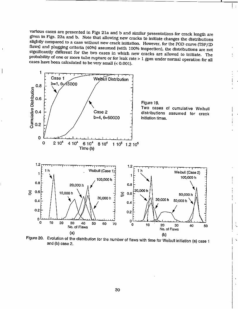
I

various cases are presented in Figs 21a and b and similar presentations for crack length are given in Figs. 22a and b. Note that allowing new cracks to initiate changes the distributions slightly compared to a case without new crack initiation. However, for the POD curve (TSP/ID flaws) and plugging criteria (40%) assumed (with 100% inspection), the distributions are not significantly different for the two cases in which new cracks are allowed to initiate. The probability of one or more tube rupture or for leak rate > I gpm under normal operation for all cases have been calculated to be very small (< 0.001).

Case 1 We' ull Distribution 08 b=l1 5000 0.8

A Figure 19.

Two cases of cumulative Weibull 0.4 Case 2 distributions assumed for crack b=4, 0=60000 initiation times.

E " 0.2

0

0 0 2104 4104= 6 104 8 104 1 105 1.2 10s5

Time (h)

1.2

1

0.8

S0.6

0.4

0.2

0-0 10 20 30 40 50 60

No. of Flaws

(a) Figure 20. Evolution of the distribution for the

and (b) case 2.

x

70 20 30 No. of Flaws

(b) number of flaws with time for Weibull initiation (a) case 1

30

.Bin size=0.05 _ No initiation

---- -Casel1 'I ~ - -Case 2

it

' '30,000 h

POD for TSP/ID Flaws

1 i~f\40% Plugging Criteria

I f 100% Inspection

S 111, ý-, ',-, -• I ,I, , I I ,

0 0.2 0.4 0.6 0.8 Crack Depth

(a)

0.8

0.6

0.4

0.2

0 2 0 0.2 0.4 0.6 0.8

Crack Depth

(b)Figure 21. Distributions of crack depth calculated without initiation and with Weibull initiation case 1 and

case 2 at (a) 30,000 h and (b) 100,000 h.

0.5

0.4

0.3

0.2

0.1

00 0.2 0.4 0.6 0.8 1 1.2 1.4 1.6

Crack Length (in.)

(a)

Bin ize=0Z& in.

I I *1 1

No initiation -Case I

--- Case 2

80,000 h

POD for TSPAD Flaws

40% Plugging Criteria

100% Inspection

0 0.2 0.4 0.6 0.8 1 1.2 Crack Length (in.)

(b)

1.4 1.6

Figure 22. Distributions of crack length calculated without initiation and with Weibull initiation case 1 and case 2 at (a) 30,000 h and (b) 80,000 h.

31

0.8

0.6

0.4

0.2

0

.Bin size=0.5 No initiation - Jl Case 1 " I ----- Case2

- 100,000 h Ii " "A j -POD for TSP/ID Flaws

- 1 40% Plugging Criteria

100% Inspection

1 1.2

x

0.5

0.4

0.3

0.2

0.1

0

Bn size=O.05 in. No initiation

-Case 1 ---- Case 2

30,000 h

\ POD for TSP/ID Flaws 40% Plugging Criteria

100% Inspection

1 1

5 Conclusions and Recommendations for Future Work

The Monte Carlo-based code CANTIA to simulate the effects of tube inspection and maintenance strategies on the safe operation of CANDU design nuclear steam generators has been updated with several new features. The ANL failure and leak rate models have been added as options. Stress corrosion crack growth can now be calculated in terms of both depth and length simultaneously The Scott and Ford-Andresen models for stress corrosion crack growth rates have been added as options. A simple residual stress model has been included.

The ANL/CANTIA code has been checked extensively for axial cracks. Several sample trial runs have been conducted to explore the effect of POD and new crack initiation on the rupture and leak rate probabilities. The circumferential crack models have not been checked as thoroughly and may require more debugging. Several other improvements in the code may be warranted in the future:

(1) Water chemistry is accounted for in the model only by the users choice of input values for crack growth and initiation parameters. More complete phenomenological models of crack initiation and growth are needed to get a more realistic picture of steam generator behavior.

(2) Currently, the initiation of new cracks is assumed to occur randomly in time, but the initiated crack is assumed to be of a fixed size independent of temperature, stress, and any other environmental parameters. A more refined initiation model should be developed in the future.

(5) Trial runs with ANL/CANTIA have shown that in the case of PWSCC it is very difficult to grow stress corrosion cracks by pressure-induced stress alone without the help of residual stress. In practice, residual stresses are almost always involved wherever early stress corrosion cracks are' detected in steam generators. The current residual stress model in ANL/CANTIA is very simplified. Because of the important role of the residual stresses, a more realistic model for residual stress should be developed.

(6) The Scott and Ford-Andresen model are reasonable phenomenological descriptions of PWSCC growth rate in the regime controlled by fracture mechanics. Other phenomenological models, such as internal oxidation model, hydrogen embrittlement model, etc. should be added. In addition better phenomenological descriptions of the growth and maturation of crack networks that cannot be described in terms of fracture mechanics need to be developed and incorporated.

(7) Flaw geometries in the current ANL/CANTIA are characterized by a depth and a length both in terms of growth and failure. Recent work at ANL and elsewhere have indicated that the "equivalent rectangular crack" method, which essentially provides an effective length and depth, can estimate the ligament rupture pressure and leak rates from fairly complex depth profiles. Whether the growth of stress corrosion cracks can be predicted or even crudely estimated from analysis of the "equivalent rectangular crack" by using fracture mechanics methodology has not yet been established. A methodology for predicting growth rates of complex stress corrosion cracks needs to be developed. Until

32

then, determining an effective length and depth through the equivalent rectangular crack method developed for integrity analyses appears to be a reasonable approach.

33

References

1. J. E. Harris, J. A. Gorman, and A.P.L. Turner, Probabilistic Methodology for Assessing Steam Generator Tube Inspection - Phase II, Report prepared by Dominion Engineering, Inc. for AECB Research Project No. 2.353.2, March 1997.

2. D. S. Kupperman, S. Bakhtlari, W. J. Shack, J. Y. Park, and S. Majumdar, "Evaluation of Eddy Current Reliability from Steam Generator Mock-up Round-Robin," NUREG/ CR-xxxx, ANL-01/22, Argonne National Laboratory, 2001.

3. J. C. Newman, Jr. and I. S. Raju ,"An empirical Stress Intensity Factor Equation for Surface Cracks." Engineering Fracture Mechanics, Vol. 15, pp. 185-192, 1981.

4. F. Erdogan, "Ductile failure theories for pressurized pipes and containers," Int. J. of Pres. Ves. & Piping, Vol. 4, pp. 253-283, 1976.

5. P. M. Scott, An Analysis of Primary Water Stress Corrosion Cracking in PWR Steam Generators, Proc. of the Specialists Meeting on Operating Experience with Steam Generators, Brussels, Belgium (Sept. 1991), pp. 5-6.

6. F. P. Ford and P. L. Andresen, Development and Use of a Predictive Model of Crack Propagation in 304/316L, A533B/A508, and Inconel 600/182 Alloys in 288'C Water, Proc. 3rd Int. Symp. on Environmental Degradation of Materials in Nuclear Power Systems-Water Reactors, Traverse City, MI, The Metallurgical Society/AIME, Warrendale, PA (1988), pp. 789-800.

7. S. Majumdar, "Assessment of Current Understanding of Mechanisms of Initiation, Arrest, and Reinitiation of tress Corrosion Cracks in PWR Steam Generator Tubing," NUREG/CR-5752, Argonne National Laboratory Report ANL-99/4, 2000.

8. S. Majumdar, K. Kasza, and J. Franklin, "Pressure and Leak Rate Tests and Models for Predicting Failure of Steam Generator tubes," NUREG/CR-6664, Argonne National Laboratory Report ANL-99/23, 2000.

9. J. M. Alzheimer, R. A. Clark, C. J. Morris, and M. Vagins, Steam Generator Tube Integrity Program Phase I Report, NUREG/CR-0718, PNL-2937, Richland, WA, Sept., 1979.

10. S. Majumdar, W. J. Shack, D.R. Diercks, K. Mruk, J. Franklin, and L. Knoblich, "Failure Behavior of Internally Pressurized Flawed and Unflawed Steam Generator Tubing at High Temperatures - Experiments and Comparison with Model Predictions," NUREG/CR-6575, ANL-97/17, Argonne, IL, 1998.

11. R. Kurihara, S. Ueda, and D. Sturm, "Estimation of the ductile unstable fracture of pipe with a circumferential surface crack subjected to bending," Nucl. Eng. Design, Vol. 106, 1988.

34

12. A. Zahoor, Ductile Fracture Handbook, Electric Power Research Institute, Palo Alto, CA, 1989.

35

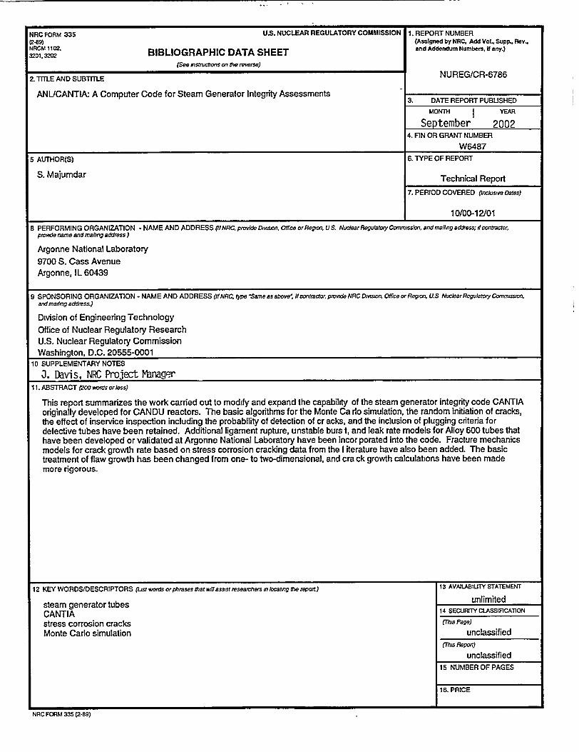
NRC FORM 335 U.S. NUCLEAR REGULATORY COMMISSION 1. REPORT NUMBER (2-89) (Assigned by NRC, Add Vol., Supp., Rev., NRCM 1102. and Addendum Numbers, If any.) 3201. BIBLIOGRAPHIC DATA SHEET

(See instuctons on the reverse)

2. TITLE AND SUBTITLE NUREG/CR-6786

ANLJCANTIA: A Computer Code for Steam Generator Integrity Assessments 3. DATE REPORT PUBUSHED

MONTH I YEAR

September 2002 4. FIN OR GRANT NUMBER

W6487

5 AUTHOR(S) 6. TYPE OF REPORT

S. Majumdar Technical Report

7. PERIOD COVERED (inclus eDates)

10/00-12/01

8 PERFORMING ORGANIZATION -NAME AND ADDRESS Vt NRC, provide Division. Office or Region. US. Nuclear Regulatory Commission, and mailing address;, i contractor. provide name and malting address )

Argonne National Laboratory 9700 S. Cass Avenue Argonne, IL 60439

9 SPONSORING ORGANIZATION - NAME AND ADDRESS (If NRC, type 'Same asabove; if contractor, provide NRC Dision, Office or Region. U.S Nuclear Regulatory Commission, and mailing address.)

Division of Engineering Technology Office of Nuclear Regulatory Research U.S. Nuclear Regulatory Commission Washington, D.C. 20555-0001

10 SUPPLEMENTARY NOTES

J. Davis, NRC Project Manager11. ABSTRACT 200 words orless)

This report summarizes the work carried out to modify and expand the capability of the steam generator integrity code CANTIA originally developed for CANDU reactors. The basic algorithms for the Monte Carlo simulation, the random initiation of cracks, the effect of inservice inspection including the probability of detection of cracks, and the inclusion of plugging criteria for defective tubes have been retained. Additional ligament rupture, unstable burs t, and leak rate models for Alloy 600 tubes that have been developed or validated at Argonne National Laboratory have been incorporated into the code. Fracture mechanics models for crack growth rate based on stress corrosion cracking data from the Iiterature have also been added. The basic treatment of flaw growth has been changed from one- to two-dimensional, and crack growth calculations have been made more rigorous.

12 KEY WORDS/DESCRIPTORS (Dst words orphrases that ww assist researchers in locating the report) 13 AVAJILABIUTY STATEMENT

steam generator tubes unlimited

CANTIA 14 SECURITY CLASSIFICATION

stress corrosion cracks (This Page)

Monte Carlo simulation unclassified (This Repo•t)

unclassified 15 NUMBER OF PAGES

16. PRICE

NRC FORM 335 (2-89)

Printed on recycled

ipaper

Federal Recycling Program

NUREG/CR-6786 ANL/CANTIA: A COMPUTER CODE FOR STEAM GENERATOR INTEGRITY ASSESSMENTS

SEPTEMBER 2002

UNITED STATES NUCLEAR REGULATORY COMMISSION

WASHINGTON, DC 20555-0001

OFFICIAL BUSINESS PENALTY FOR PRIVATE USE, $300