HSEHealth & Safety

Executive

Interpretation of full-scale monitoringdata from a jack-up rig

Prepared by MSL Engineering Ltdfor the Health and Safety Executive

OFFSHORE TECHNOLOGY REPORT

2001/035

HSEHealth & Safety

Executive

Interpretation of full-scale monitoringdata from a jack-up rig

MSL Engineering LtdMSL House

5-7 High StreetSunninghill

AscotBerkshire SL5 9NQ

United Kingdom

HSE BOOKS

ii

© Crown copyright 2002Applications for reproduction should be made in writing to:Copyright Unit, Her Majesty’s Stationery Office,St Clements House, 2-16 Colegate, Norwich NR3 1BQ

First published 2002

ISBN 0 7176 2298 3

All rights reserved. No part of this publication may bereproduced, stored in a retrieval system, or transmittedin any form or by any means (electronic, mechanical,photocopying, recording or otherwise) without the priorwritten permission of the copyright owner.

This report is made available by the Health and SafetyExecutive as part of a series of reports of work which hasbeen supported by funds provided by the Executive.Neither the Executive, nor the contractors concernedassume any liability for the reports nor do theynecessarily reflect the views or policy of the Executive.

iii

FOREWORD

This document summarises a study undertaken by MSL Engineering Ltd for the Health and Safety Executive to determine the foundation fixity of the Maersk Endurer Jack-Up rig from measured data. This particular Jack-Up does not have spudcan skirts, and therefore the results complement earlier studies on Jack-Ups having skirts. Several sea states from two storms were examined so that conclusions could be drawn on the possibility of foundation softening occurring during a storm. Foundation fixity was inferred from the observed natural period of the structure. Comparisons of measured maximum displacement with predicted values using the inferred fixity levels have also been made.

iv

v

CONTENTS FOREWORD iii CONTENTS v

1. SUMMARY 1

2. INTRODUCTION 2

3. DESCRIPTION OF UNIT 4 3.1 Structure 4 3.2 Foundations 4

4. REDUCTION OF MONITORED DATA 5 4.1 Introduction 5 4.2 Metocean Data 5 4.3 Structural Response Data 6

5. PREDICTION OF STRUCTURAL RESPONSE 8 5.1 Model Description 8 5.2 Foundation Fixity 9 5.3 Prediction of Structural Response using FE Model 10 5.4 Metocean Data 11

6. RESULTS 12 6.1 Measured Structural Natural Periods 12 6.2 Equivalent Foundation Fixity to Match Monitored Response 12 6.3 Predicted Displacements 13 6.4 Comparison of Predicted and Measured Displacements 13 6.5 Maximum Foundation Loads 17

7. CONCLUSIONS 18

8. REFERENCES 19

vi

1

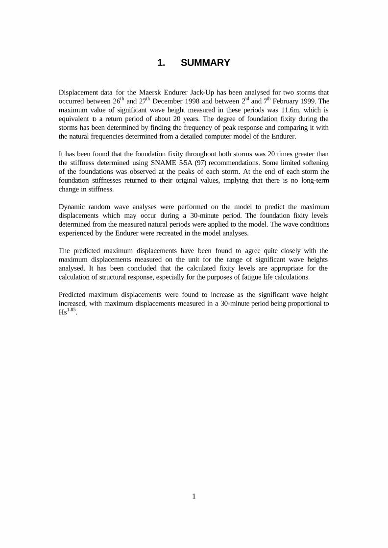
1. SUMMARY

Displacement data for the Maersk Endurer Jack-Up has been analysed for two storms that occurred between 26th and 27th December 1998 and between 2nd and 7th February 1999. The maximum value of significant wave height measured in these periods was 11.6m, which is equivalent to a return period of about 20 years. The degree of foundation fixity during the storms has been determined by finding the frequency of peak response and comparing it with the natural frequencies determined from a detailed computer model of the Endurer. It has been found that the foundation fixity throughout both storms was 20 times greater than the stiffness determined using SNAME 5-5A (97) recommendations. Some limited softening of the foundations was observed at the peaks of each storm. At the end of each storm the foundation stiffnesses returned to their original values, implying that there is no long-term change in stiffness. Dynamic random wave analyses were performed on the model to predict the maximum displacements which may occur during a 30-minute period. The foundation fixity levels determined from the measured natural periods were applied to the model. The wave conditions experienced by the Endurer were recreated in the model analyses. The predicted maximum displacements have been found to agree quite closely with the maximum displacements measured on the unit for the range of significant wave heights analysed. It has been concluded that the calculated fixity levels are appropriate for the calculation of structural response, especially for the purposes of fatigue life calculations. Predicted maximum displacements were found to increase as the significant wave height increased, with maximum displacements measured in a 30-minute period being proportional to Hs1.85.

2

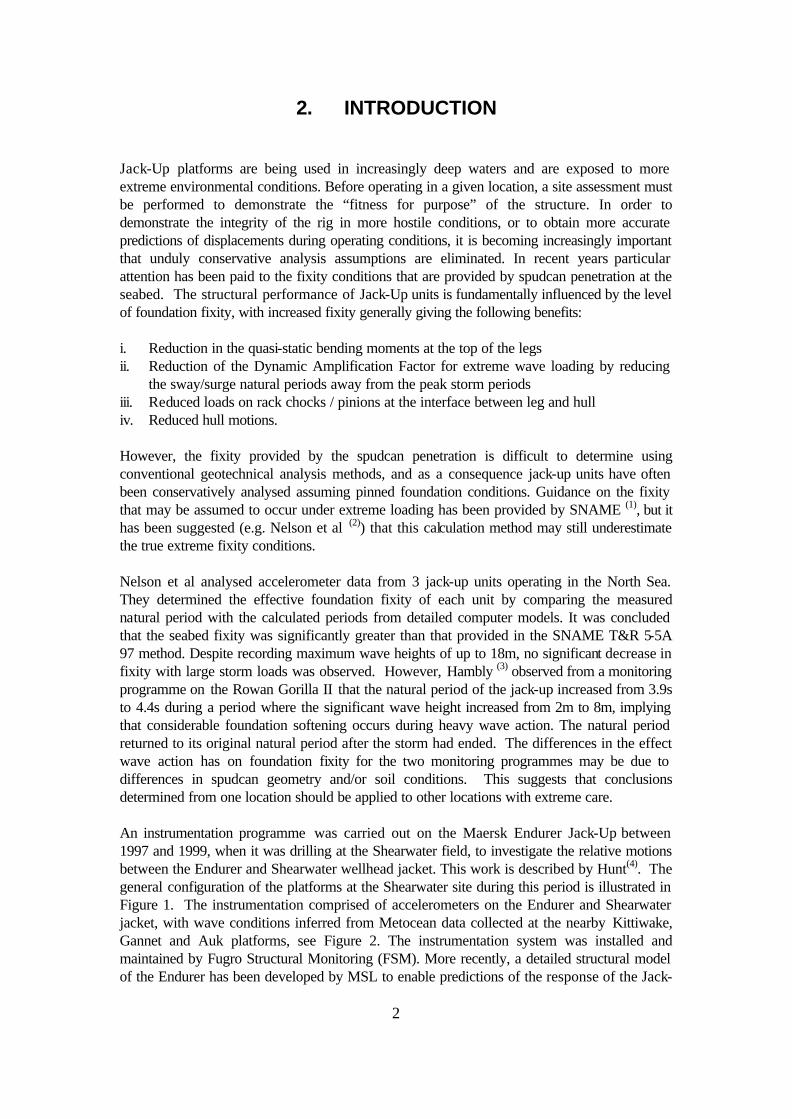
2. INTRODUCTION Jack-Up platforms are being used in increasingly deep waters and are exposed to more extreme environmental conditions. Before operating in a given location, a site assessment must be performed to demonstrate the “fitness for purpose” of the structure. In order to demonstrate the integrity of the rig in more hostile conditions, or to obtain more accurate predictions of displacements during operating conditions, it is becoming increasingly important that unduly conservative analysis assumptions are eliminated. In recent years particular attention has been paid to the fixity conditions that are provided by spudcan penetration at the seabed. The structural performance of Jack-Up units is fundamentally influenced by the level of foundation fixity, with increased fixity generally giving the following benefits: i. Reduction in the quasi-static bending moments at the top of the legs ii. Reduction of the Dynamic Amplification Factor for extreme wave loading by reducing

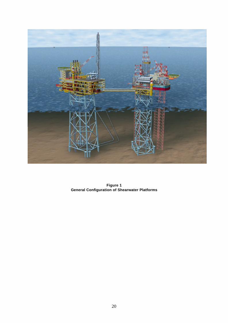
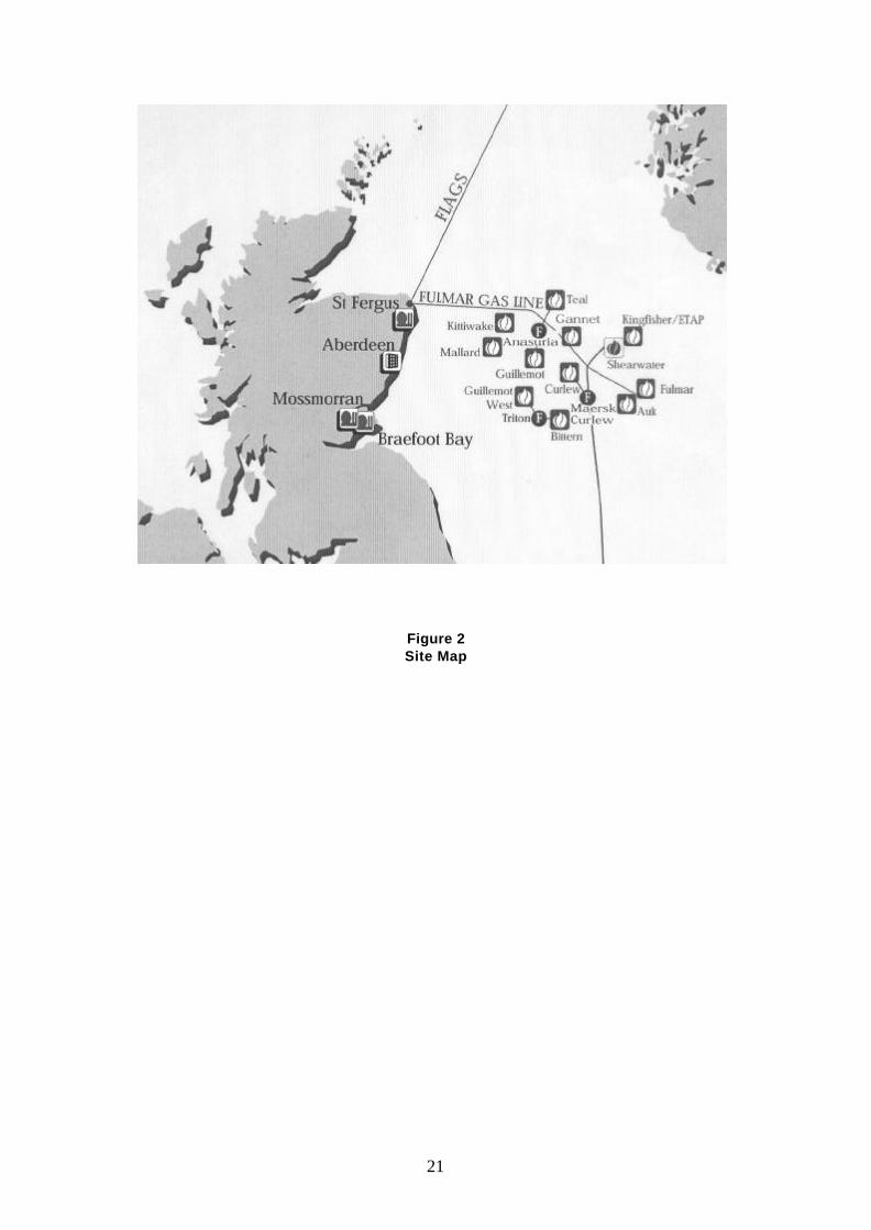
the sway/surge natural periods away from the peak storm periods iii. Reduced loads on rack chocks / pinions at the interface between leg and hull iv. Reduced hull motions. However, the fixity provided by the spudcan penetration is difficult to determine using conventional geotechnical analysis methods, and as a consequence jack-up units have often been conservatively analysed assuming pinned foundation conditions. Guidance on the fixity that may be assumed to occur under extreme loading has been provided by SNAME (1), but it has been suggested (e.g. Nelson et al (2)) that this calculation method may still underestimate the true extreme fixity conditions. Nelson et al analysed accelerometer data from 3 jack-up units operating in the North Sea. They determined the effective foundation fixity of each unit by comparing the measured natural period with the calculated periods from detailed computer models. It was concluded that the seabed fixity was significantly greater than that provided in the SNAME T&R 5-5A 97 method. Despite recording maximum wave heights of up to 18m, no significant decrease in fixity with large storm loads was observed. However, Hambly (3) observed from a monitoring programme on the Rowan Gorilla II that the natural period of the jack-up increased from 3.9s to 4.4s during a period where the significant wave height increased from 2m to 8m, implying that considerable foundation softening occurs during heavy wave action. The natural period returned to its original natural period after the storm had ended. The differences in the effect wave action has on foundation fixity for the two monitoring programmes may be due to differences in spudcan geometry and/or soil conditions. This suggests that conclusions determined from one location should be applied to other locations with extreme care. An instrumentation programme was carried out on the Maersk Endurer Jack-Up between 1997 and 1999, when it was drilling at the Shearwater field, to investigate the relative motions between the Endurer and Shearwater wellhead jacket. This work is described by Hunt(4). The general configuration of the platforms at the Shearwater site during this period is illustrated in Figure 1. The instrumentation comprised of accelerometers on the Endurer and Shearwater jacket, with wave conditions inferred from Metocean data collected at the nearby Kittiwake, Gannet and Auk platforms, see Figure 2. The instrumentation system was installed and maintained by Fugro Structural Monitoring (FSM). More recently, a detailed structural model of the Endurer has been developed by MSL to enable predictions of the response of the Jack-

3

Up in the various seastates it encountered in the monitoring period. This has allowed the following objectives to be achieved: i. Use the instrumented data to determine the natural period of the Endurer for selected sea

states and hence to infer the degree of foundation fixity from the structural model of the Endurer.

ii. Determine if significant softening of the foundations occurred during storm conditions, and if the foundation stiffness returns to its initial value after the storm.

iii. Compare the inferred fixity conditions for each sea state with fixities calculated using established methods (e.g. SNAME method).

iv. Using the inferred fixity conditions from (i) and a Wave Response Analysis, calculate the most likely maximum displacements to occur for each seastate in a 30-minute period. Compare the measured maximum displacements to the calculated values.

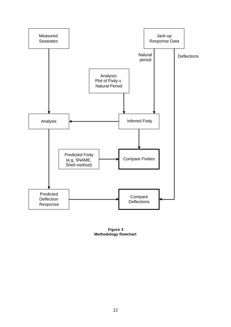
A flow diagram of the analysis methodology is shown in Figure 3.

4

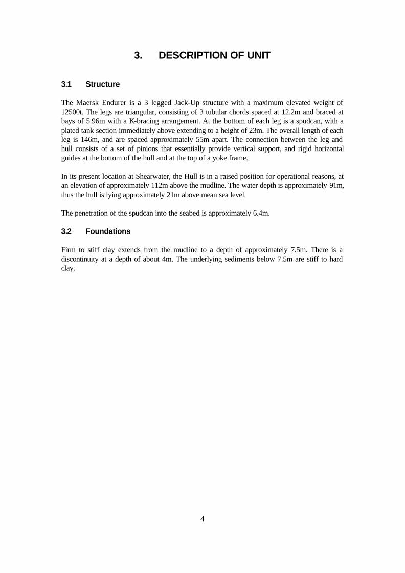
3. DESCRIPTION OF UNIT 3.1 Structure The Maersk Endurer is a 3 legged Jack-Up structure with a maximum elevated weight of 12500t. The legs are triangular, consisting of 3 tubular chords spaced at 12.2m and braced at bays of 5.96m with a K-bracing arrangement. At the bottom of each leg is a spudcan, with a plated tank section immediately above extending to a height of 23m. The overall length of each leg is 146m, and are spaced approximately 55m apart. The connection between the leg and hull consists of a set of pinions that essentially provide vertical support, and rigid horizontal guides at the bottom of the hull and at the top of a yoke frame. In its present location at Shearwater, the Hull is in a raised position for operational reasons, at an elevation of approximately 112m above the mudline. The water depth is approximately 91m, thus the hull is lying approximately 21m above mean sea level. The penetration of the spudcan into the seabed is approximately 6.4m. 3.2 Foundations Firm to stiff clay extends from the mudline to a depth of approximately 7.5m. There is a discontinuity at a depth of about 4m. The underlying sediments below 7.5m are stiff to hard clay.

5

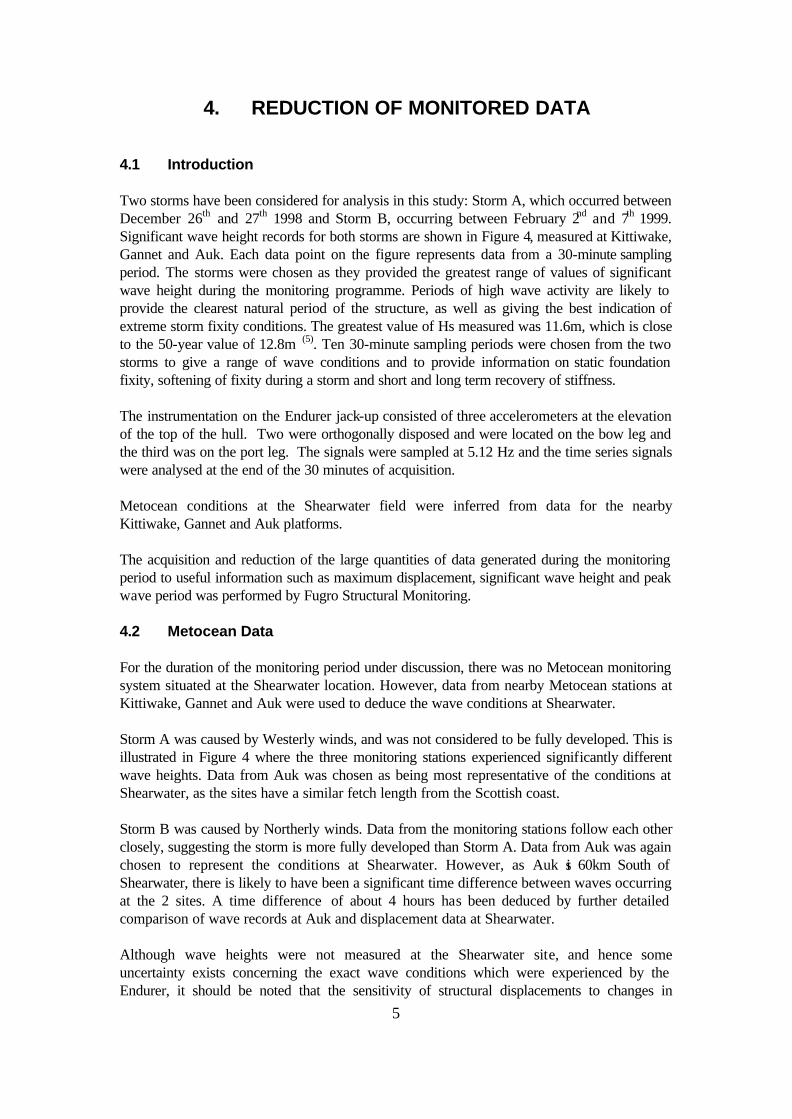
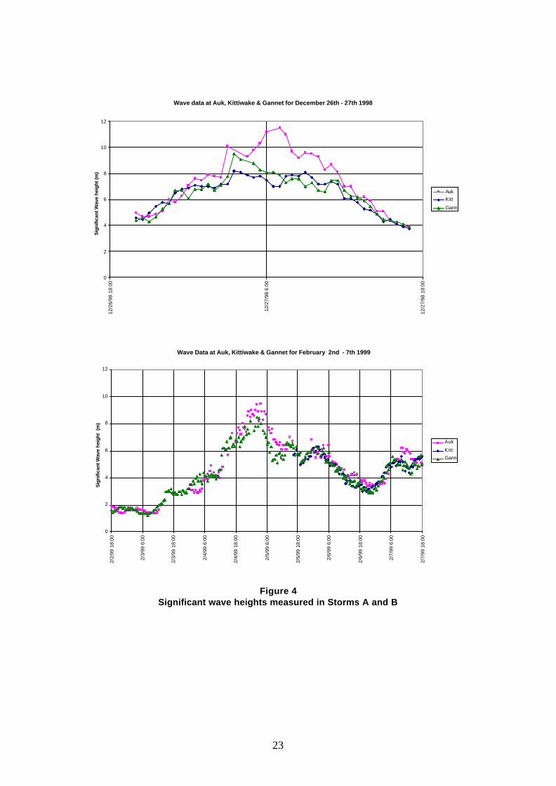
4. REDUCTION OF MONITORED DATA 4.1 Introduction Two storms have been considered for analysis in this study: Storm A, which occurred between December 26th and 27th 1998 and Storm B, occurring between February 2nd and 7th 1999. Significant wave height records for both storms are shown in Figure 4, measured at Kittiwake, Gannet and Auk. Each data point on the figure represents data from a 30-minute sampling period. The storms were chosen as they provided the greatest range of values of significant wave height during the monitoring programme. Periods of high wave activity are likely to provide the clearest natural period of the structure, as well as giving the best indication of extreme storm fixity conditions. The greatest value of Hs measured was 11.6m, which is close to the 50-year value of 12.8m (5). Ten 30-minute sampling periods were chosen from the two storms to give a range of wave conditions and to provide information on static foundation fixity, softening of fixity during a storm and short and long term recovery of stiffness. The instrumentation on the Endurer jack-up consisted of three accelerometers at the elevation of the top of the hull. Two were orthogonally disposed and were located on the bow leg and the third was on the port leg. The signals were sampled at 5.12 Hz and the time series signals were analysed at the end of the 30 minutes of acquisition. Metocean conditions at the Shearwater field were inferred from data for the nearby Kittiwake, Gannet and Auk platforms. The acquisition and reduction of the large quantities of data generated during the monitoring period to useful information such as maximum displacement, significant wave height and peak wave period was performed by Fugro Structural Monitoring. 4.2 Metocean Data For the duration of the monitoring period under discussion, there was no Metocean monitoring system situated at the Shearwater location. However, data from nearby Metocean stations at Kittiwake, Gannet and Auk were used to deduce the wave conditions at Shearwater. Storm A was caused by Westerly winds, and was not considered to be fully developed. This is illustrated in Figure 4 where the three monitoring stations experienced significantly different wave heights. Data from Auk was chosen as being most representative of the conditions at Shearwater, as the sites have a similar fetch length from the Scottish coast. Storm B was caused by Northerly winds. Data from the monitoring stations follow each other closely, suggesting the storm is more fully developed than Storm A. Data from Auk was again chosen to represent the conditions at Shearwater. However, as Auk is 60km South of Shearwater, there is likely to have been a significant time difference between waves occurring at the 2 sites. A time difference of about 4 hours has been deduced by further detailed comparison of wave records at Auk and displacement data at Shearwater. Although wave heights were not measured at the Shearwater site, and hence some uncertainty exists concerning the exact wave conditions which were experienced by the Endurer, it should be noted that the sensitivity of structural displacements to changes in

6

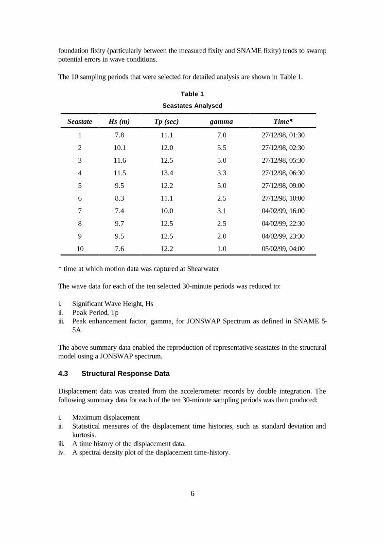
foundation fixity (particularly between the measured fixity and SNAME fixity) tends to swamp potential errors in wave conditions. The 10 sampling periods that were selected for detailed analysis are shown in Table 1.

Table 1

Seastates Analysed

Seastate Hs (m) Tp (sec) gamma Time*

1 7.8 11.1 7.0 27/12/98, 01:30

2 10.1 12.0 5.5 27/12/98, 02:30

3 11.6 12.5 5.0 27/12/98, 05:30

4 11.5 13.4 3.3 27/12/98, 06:30

5 9.5 12.2 5.0 27/12/98, 09:00

6 8.3 11.1 2.5 27/12/98, 10:00

7 7.4 10.0 3.1 04/02/99, 16:00

8 9.7 12.5 2.5 04/02/99, 22:30

9 9.5 12.5 2.0 04/02/99, 23:30

10 7.6 12.2 1.0 05/02/99, 04:00

* time at which motion data was captured at Shearwater The wave data for each of the ten selected 30-minute periods was reduced to: i. Significant Wave Height, Hs ii. Peak Period, Tp iii. Peak enhancement factor, gamma, for JONSWAP Spectrum as defined in SNAME 5-

5A. The above summary data enabled the reproduction of representative seastates in the structural model using a JONSWAP spectrum. 4.3 Structural Response Data Displacement data was created from the accelerometer records by double integration. The following summary data for each of the ten 30-minute sampling periods was then produced: i. Maximum displacement ii. Statistical measures of the displacement time histories, such as standard deviation and

kurtosis. iii. A time history of the displacement data. iv. A spectral density plot of the displacement time-history.

7

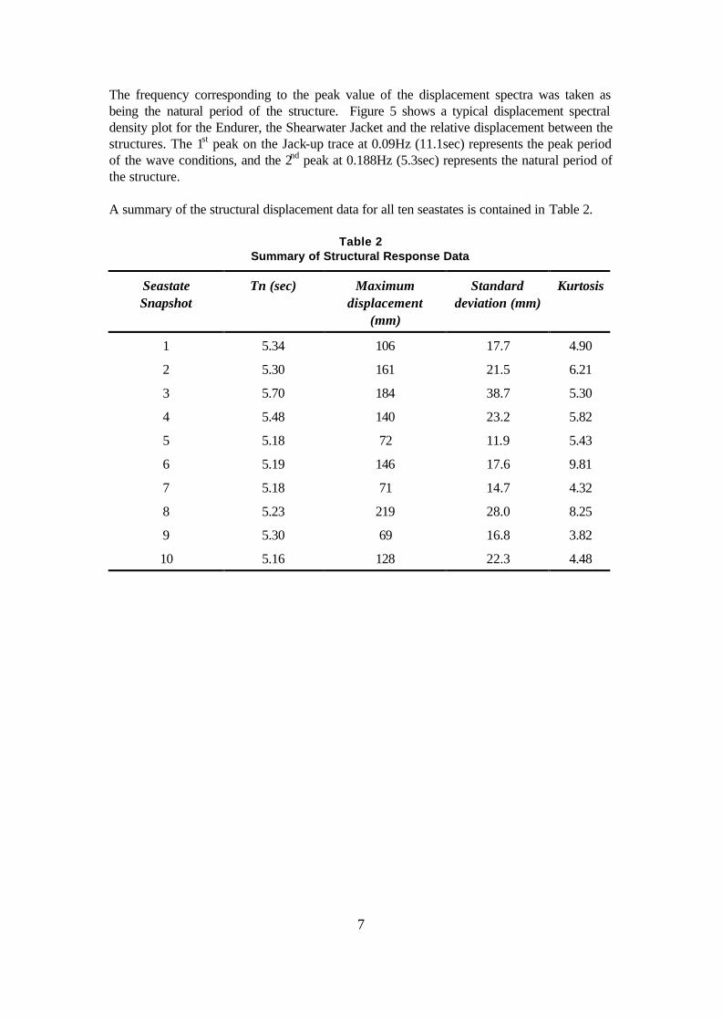
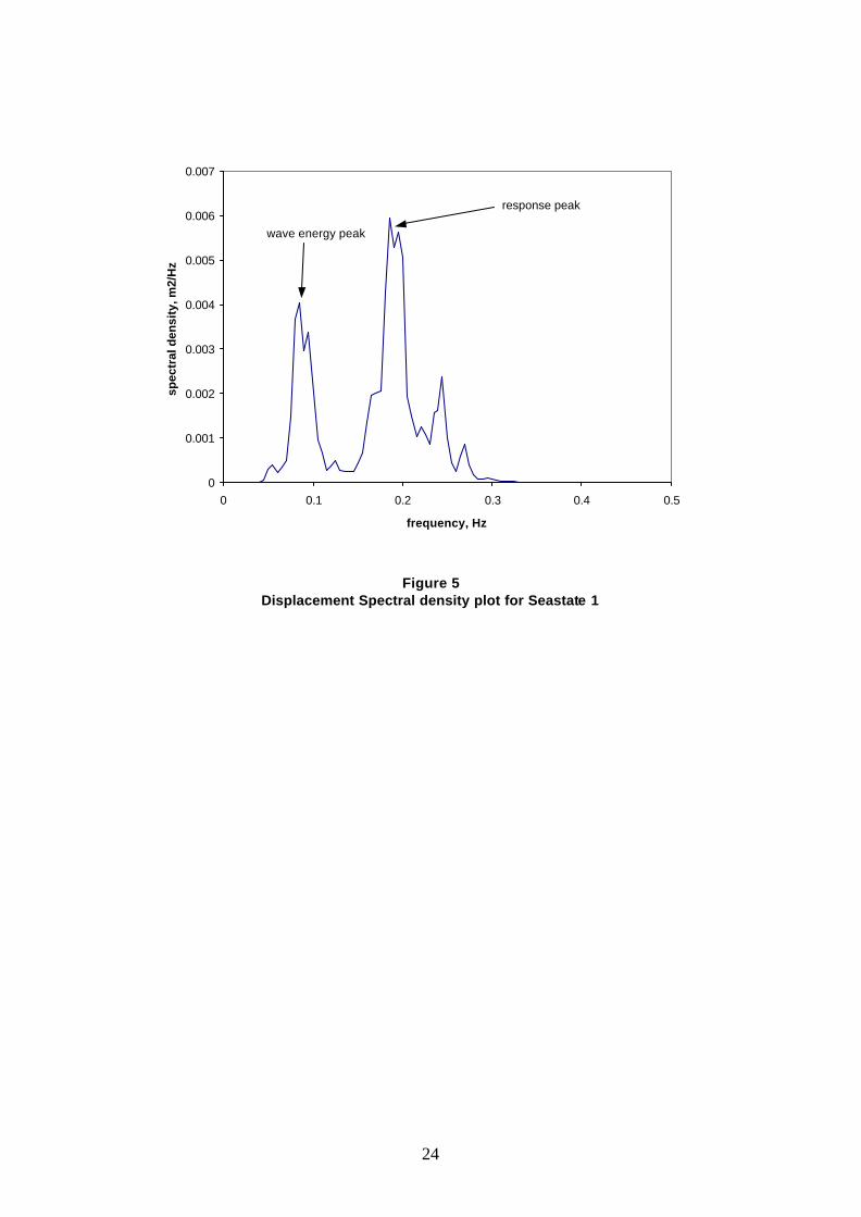
The frequency corresponding to the peak value of the displacement spectra was taken as being the natural period of the structure. Figure 5 shows a typical displacement spectral density plot for the Endurer, the Shearwater Jacket and the relative displacement between the structures. The 1st peak on the Jack-up trace at 0.09Hz (11.1sec) represents the peak period of the wave conditions, and the 2nd peak at 0.188Hz (5.3sec) represents the natural period of the structure. A summary of the structural displacement data for all ten seastates is contained in Table 2.

Table 2 Summary of Structural Response Data

Seastate Snapshot

Tn (sec) Maximum displacement

(mm)

Standard deviation (mm)

Kurtosis

1 5.34 106 17.7 4.90

2 5.30 161 21.5 6.21

3 5.70 184 38.7 5.30

4 5.48 140 23.2 5.82

5 5.18 72 11.9 5.43

6 5.19 146 17.6 9.81

7 5.18 71 14.7 4.32

8 5.23 219 28.0 8.25

9 5.30 69 16.8 3.82

10 5.16 128 22.3 4.48

8

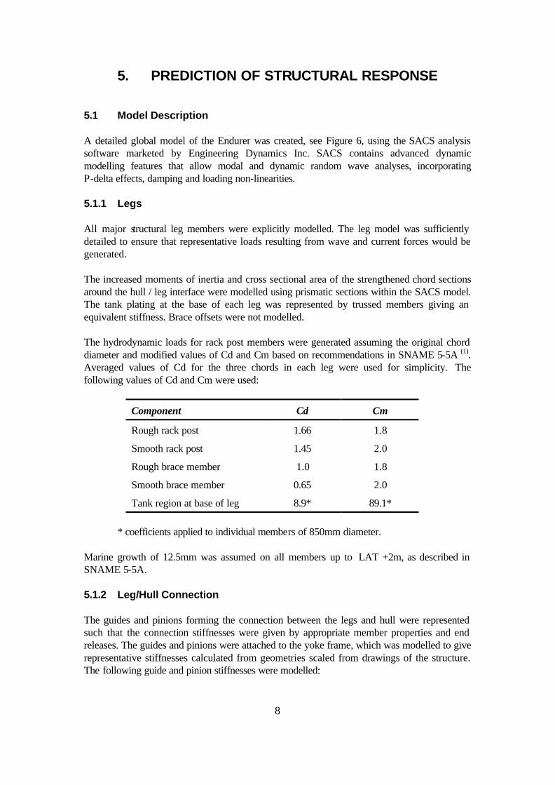
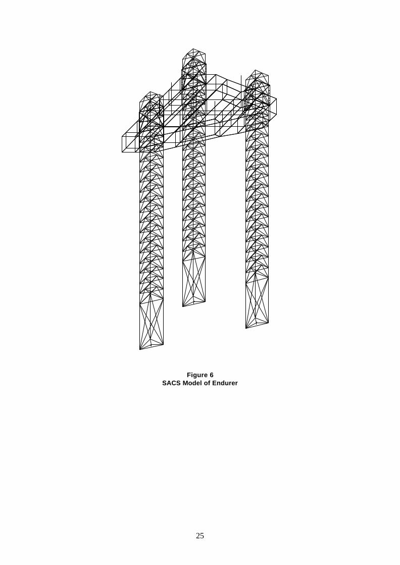
5. PREDICTION OF STRUCTURAL RESPONSE 5.1 Model Description A detailed global model of the Endurer was created, see Figure 6, using the SACS analysis software marketed by Engineering Dynamics Inc. SACS contains advanced dynamic modelling features that allow modal and dynamic random wave analyses, incorporating P-delta effects, damping and loading non-linearities. 5.1.1 Legs All major structural leg members were explicitly modelled. The leg model was sufficiently detailed to ensure that representative loads resulting from wave and current forces would be generated. The increased moments of inertia and cross sectional area of the strengthened chord sections around the hull / leg interface were modelled using prismatic sections within the SACS model. The tank plating at the base of each leg was represented by trussed members giving an equivalent stiffness. Brace offsets were not modelled. The hydrodynamic loads for rack post members were generated assuming the original chord diameter and modified values of Cd and Cm based on recommendations in SNAME 5-5A (1). Averaged values of Cd for the three chords in each leg were used for simplicity. The following values of Cd and Cm were used:

Component Cd Cm

Rough rack post 1.66 1.8

Smooth rack post 1.45 2.0

Rough brace member 1.0 1.8

Smooth brace member 0.65 2.0

Tank region at base of leg 8.9* 89.1*

* coefficients applied to individual members of 850mm diameter.

Marine growth of 12.5mm was assumed on all members up to LAT +2m, as described in SNAME 5-5A. 5.1.2 Leg/Hull Connection The guides and pinions forming the connection between the legs and hull were represented such that the connection stiffnesses were given by appropriate member properties and end releases. The guides and pinions were attached to the yoke frame, which was modelled to give representative stiffnesses calculated from geometries scaled from drawings of the structure. The following guide and pinion stiffnesses were modelled:

9

Element Stiffness

Upper Guide 86.0 x 103 t/m

Lower Guide 500 x 103 t/m

Vertical 75.0 x 103 t/m Pinions

Horizontal 35.1 x 103 t/m

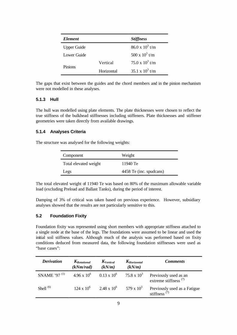
The gaps that exist between the guides and the chord members and in the pinion mechanism were not modelled in these analyses. 5.1.3 Hull The hull was modelled using plate elements. The plate thicknesses were chosen to reflect the true stiffness of the bulkhead stiffnesses including stiffeners. Plate thicknesses and stiffener geometries were taken directly from available drawings. 5.1.4 Analyses Criteria The structure was analysed for the following weights:

Component Weight

Total elevated weight 11940 Te

Legs 4458 Te (inc. spudcans)

The total elevated weight of 11940 Te was based on 80% of the maximum allowable variable load (excluding Preload and Ballast Tanks), during the period of interest. Damping of 3% of critical was taken based on previous experience. However, subsidiary analyses showed that the results are not particularly sensitive to this. 5.2 Foundation Fixity Foundation fixity was represented using short members with appropriate stiffness attached to a single node at the base of the legs. The foundations were assumed to be linear and used the initial soil stiffness values. Although much of the analysis was performed based on fixity conditions deduced from measured data, the following foundation stiffnesses were used as “base cases”:

Derivation KRotational

(kNm/rad) KVertical

(kN/m) KHorizontal

(kN/m) Comments

SNAME ’97 (1) 4.96 x 106 0.13 x 106 75.8 x 103 Previously used as an extreme stiffness (7)

Shell (6) 124 x 106 2.48 x 106 579 x 103 Previously used as a Fatigue stiffness (7)

10

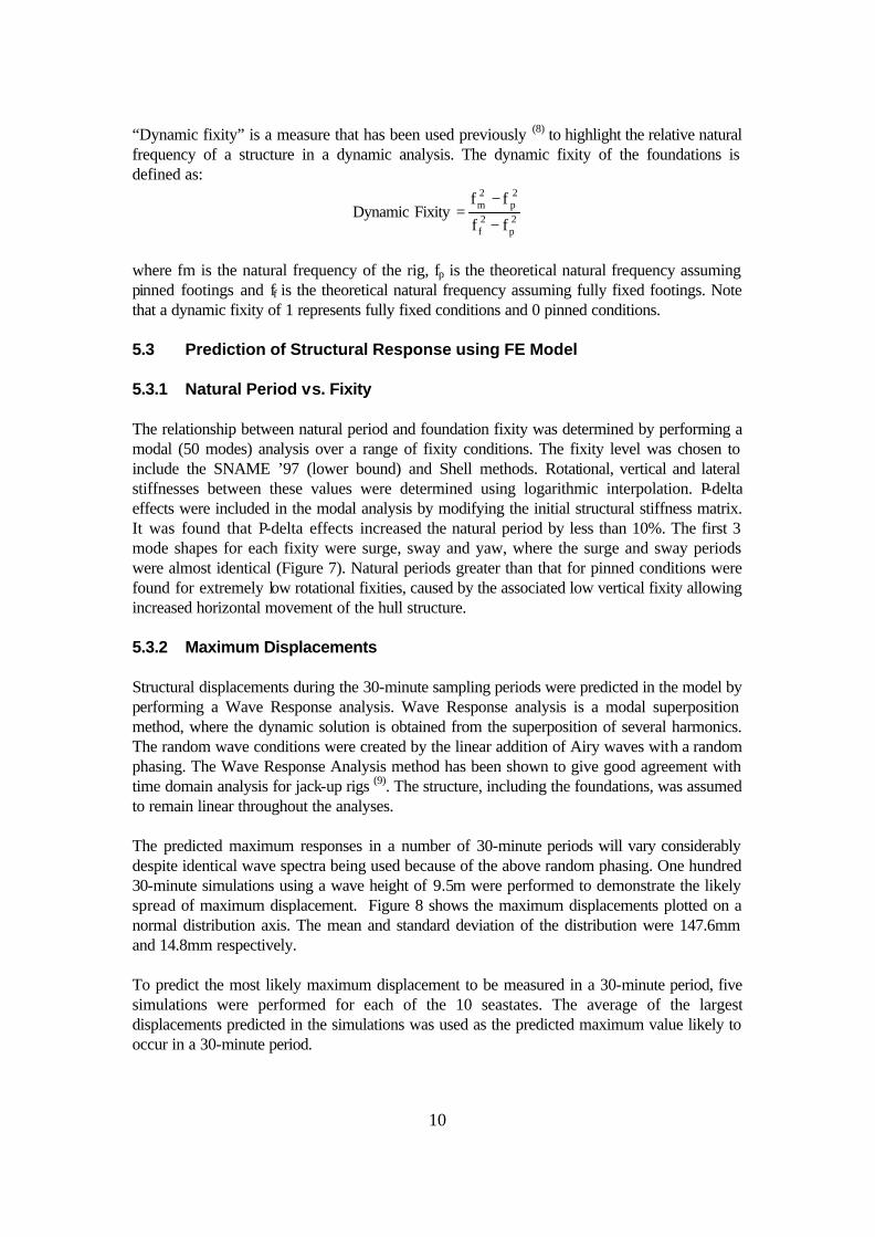
“Dynamic fixity” is a measure that has been used previously (8) to highlight the relative natural frequency of a structure in a dynamic analysis. The dynamic fixity of the foundations is defined as:

2p

2f

2p

2m

ff

ffFixity Dynamic

−

−=

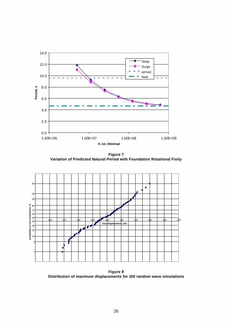
where fm is the natural frequency of the rig, fp is the theoretical natural frequency assuming pinned footings and ff is the theoretical natural frequency assuming fully fixed footings. Note that a dynamic fixity of 1 represents fully fixed conditions and 0 pinned conditions. 5.3 Prediction of Structural Response using FE Model 5.3.1 Natural Period vs. Fixity The relationship between natural period and foundation fixity was determined by performing a modal (50 modes) analysis over a range of fixity conditions. The fixity level was chosen to include the SNAME ’97 (lower bound) and Shell methods. Rotational, vertical and lateral stiffnesses between these values were determined using logarithmic interpolation. P-delta effects were included in the modal analysis by modifying the initial structural stiffness matrix. It was found that P-delta effects increased the natural period by less than 10%. The first 3 mode shapes for each fixity were surge, sway and yaw, where the surge and sway periods were almost identical (Figure 7). Natural periods greater than that for pinned conditions were found for extremely low rotational fixities, caused by the associated low vertical fixity allowing increased horizontal movement of the hull structure. 5.3.2 Maximum Displacements Structural displacements during the 30-minute sampling periods were predicted in the model by performing a Wave Response analysis. Wave Response analysis is a modal superposition method, where the dynamic solution is obtained from the superposition of several harmonics. The random wave conditions were created by the linear addition of Airy waves with a random phasing. The Wave Response Analysis method has been shown to give good agreement with time domain analysis for jack-up rigs (9). The structure, including the foundations, was assumed to remain linear throughout the analyses. The predicted maximum responses in a number of 30-minute periods will vary considerably despite identical wave spectra being used because of the above random phasing. One hundred 30-minute simulations using a wave height of 9.5m were performed to demonstrate the likely spread of maximum displacement. Figure 8 shows the maximum displacements plotted on a normal distribution axis. The mean and standard deviation of the distribution were 147.6mm and 14.8mm respectively. To predict the most likely maximum displacement to be measured in a 30-minute period, five simulations were performed for each of the 10 seastates. The average of the largest displacements predicted in the simulations was used as the predicted maximum value likely to occur in a 30-minute period.

11

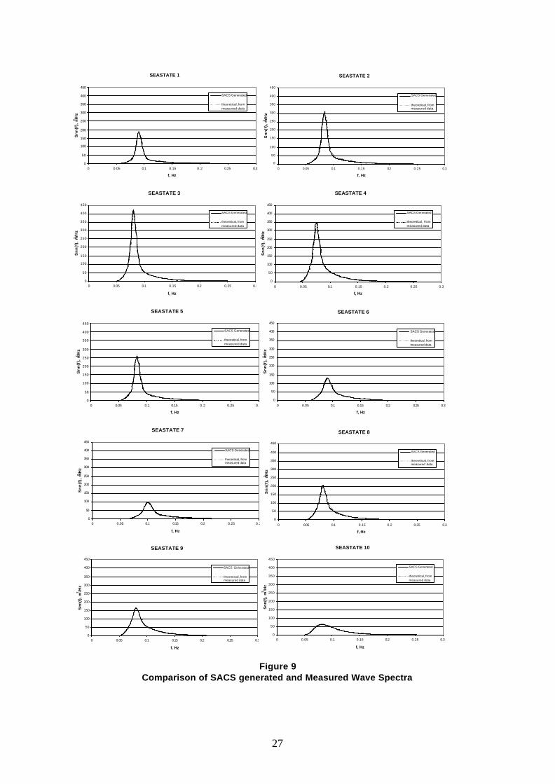
5.4 Metocean Data The measured Metocean data, reduced to the JONSWAP parameters Hs, Tp and gamma in Table 1, were provided by SHELL UK. These seastates were reproduced as closely as possible in the SACS analyses. The closeness of fit between the Metocean spectra and the spectra created from the analysis by reconverting the generated wave time-history back into the frequency domain is illustrated in Figure 9. Current was not applied in the model. Displacement data derived from accelerometer traces can only measure transient displacements and hence the displacements due to current would not be present in the maximum measured displacements. The effect that current would have on the apparent wave length has not been considered in this analysis. Wind loading has not been considered for similar reasons. (Note: The base shear caused by a 50-year wind is approximately 25% of the wave + current base shear.)

12

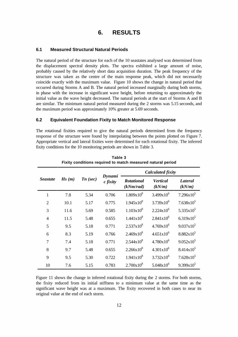
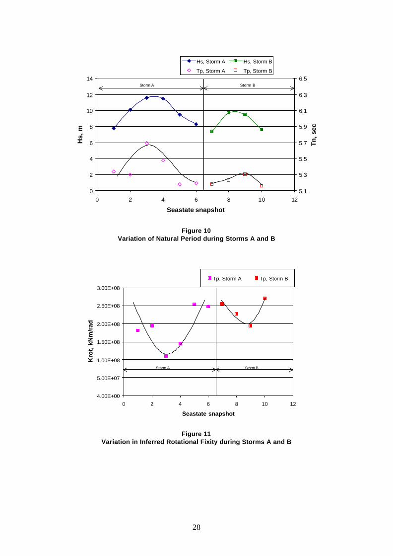
6. RESULTS 6.1 Measured Structural Natural Periods The natural period of the structure for each of the 10 seastates analysed was determined from the displacement spectral density plots. The spectra exhibited a large amount of noise, probably caused by the relatively short data acquisition duration. The peak frequency of the structure was taken as the centre of the main response peak, which did not necessarily coincide exactly with the maximum value. Figure 10 shows the change in natural period that occurred during Storms A and B. The natural period increased marginally during both storms, in phase with the increase in significant wave height, before returning to approximately the initial value as the wave height decreased. The natural periods at the start of Storms A and B are similar. The minimum natural period measured during the 2 storms was 5.15 seconds, and the maximum period was approximately 10% greater at 5.69 seconds. 6.2 Equivalent Foundation Fixity to Match Monitored Response The rotational fixities required to give the natural periods determined from the frequency response of the structure were found by interpolating between the points plotted on Figure 7. Appropriate vertical and lateral fixities were determined for each rotational fixity. The inferred fixity conditions for the 10 monitoring periods are shown in Table 3.

Table 3 Fixity conditions required to match measured natural period

Calculated fixity

Seastate Hs (m) Tn (sec) Dynamic fixity Rotational

(kNm/rad) Vertical (kN/m)

Lateral (kN/m)

1 7.8 5.34 0.706 1.809x108 3.499x106 7.296x105

2 10.1 5.17 0.775 1.945x108 3.739x106 7.638x105

3 11.6 5.69 0.585 1.103x108 2.224x106 5.335x105

4 11.5 5.48 0.655 1.441x108 2.841x106 6.319x105

5 9.5 5.18 0.771 2.537x108 4.769x106 9.037x105

6 8.3 5.19 0.766 2.469x108 4.651x106 8.882x105

7 7.4 5.18 0.771 2.544x108 4.780x106 9.052x105

8 9.7 5.48 0.655 2.266x108 4.301x106 8.414x105

9 9.5 5.30 0.722 1.941x108 3.732x106 7.628x105

10 7.6 5.15 0.783 2.700x108 5.048x106 9.399x105

Figure 11 shows the change in inferred rotational fixity during the 2 storms. For both storms, the fixity reduced from its initial stiffness to a minimum value at the same time as the significant wave height was at a maximum. The fixity recovered in both cases to near its original value at the end of each storm.

13

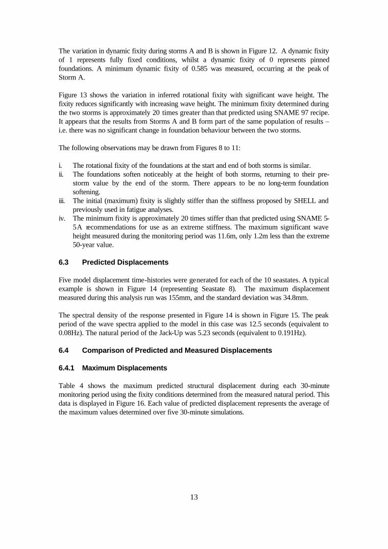
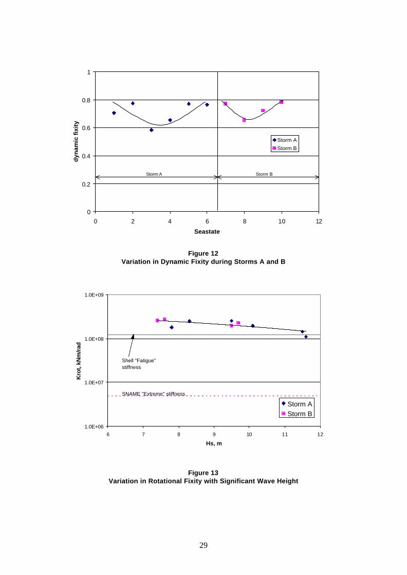
The variation in dynamic fixity during storms A and B is shown in Figure 12. A dynamic fixity of 1 represents fully fixed conditions, whilst a dynamic fixity of 0 represents pinned foundations. A minimum dynamic fixity of 0.585 was measured, occurring at the peak of Storm A. Figure 13 shows the variation in inferred rotational fixity with significant wave height. The fixity reduces significantly with increasing wave height. The minimum fixity determined during the two storms is approximately 20 times greater than that predicted using SNAME 97 recipe. It appears that the results from Storms A and B form part of the same population of results – i.e. there was no significant change in foundation behaviour between the two storms. The following observations may be drawn from Figures 8 to 11: i. The rotational fixity of the foundations at the start and end of both storms is similar. ii. The foundations soften noticeably at the height of both storms, returning to their pre-

storm value by the end of the storm. There appears to be no long-term foundation softening.

iii. The initial (maximum) fixity is slightly stiffer than the stiffness proposed by SHELL and previously used in fatigue analyses.

iv. The minimum fixity is approximately 20 times stiffer than that predicted using SNAME 5-5A recommendations for use as an extreme stiffness. The maximum significant wave height measured during the monitoring period was 11.6m, only 1.2m less than the extreme 50-year value.

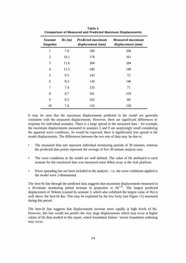
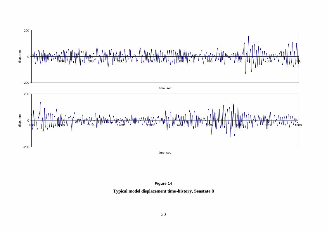
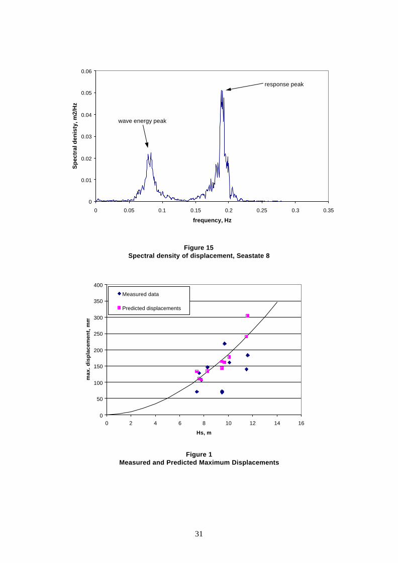
6.3 Predicted Displacements Five model displacement time-histories were generated for each of the 10 seastates. A typical example is shown in Figure 14 (representing Seastate 8). The maximum displacement measured during this analysis run was 155mm, and the standard deviation was 34.8mm. The spectral density of the response presented in Figure 14 is shown in Figure 15. The peak period of the wave spectra applied to the model in this case was 12.5 seconds (equivalent to 0.08Hz). The natural period of the Jack-Up was 5.23 seconds (equivalent to 0.191Hz). 6.4 Comparison of Predicted and Measured Displacements 6.4.1 Maximum Displacements Table 4 shows the maximum predicted structural displacement during each 30-minute monitoring period using the fixity conditions determined from the measured natural period. This data is displayed in Figure 16. Each value of predicted displacement represents the average of the maximum values determined over five 30-minute simulations.

14

Table 4

Comparison of Measured and Predicted Maximum Displacements

Seastate Snapshot

Hs (m) Predicted maximum displacement (mm)

Measured maximum displacement (mm)

1 7.8 108 106

2 10.1 178 161

3 11.6 304 184

4 11.5 240 140

5 9.5 143 72

6 8.3 134 146

7 7.4 133 71

8 9.7 161 219

9 9.5 163 69

10 7.6 110 128

It may be seen that the maximum displacements predicted in the model are generally consistent with the measured displacements. However, there are significant differences in response for individual seastates. There is a large spread in the measured data – for example, the maximum displacements measured in seastates 5 and 9 are surprisingly small considering the apparent wave conditions. As would be expected, there is significantly less spread in the model displacements. The differences between the two sets of data may be due to: • The measured data sets represent individual monitoring periods of 30 minutes, whereas

the predicted data points represent the average of five 30-minute analysis runs. • The wave conditions in the model are well defined. The value of Hs attributed to each

seastate for the monitored data was measured some 60km away at the Auk platform. • Wave spreading has not been included in the analysis – i.e. the wave conditions applied to

the model were 2-dimensional. The best-fit line through the predicted data suggests that maximum displacements measured in a 30-minute monitoring period increase in proportion to Hs1.85. The largest predicted displacement of 304mm (caused by seastate 3, which also exhibited the largest value of Hs) is well above the best-fit line. This may be explained by the low fixity (see Figure 11) measured during this period. The best-fit line suggests that displacements increase more rapidly at high levels of Hs. However, this line would not predict the very large displacements which may occur at higher values of Hs than studied in this report, where foundation failure / severe foundation softening may occur.

15

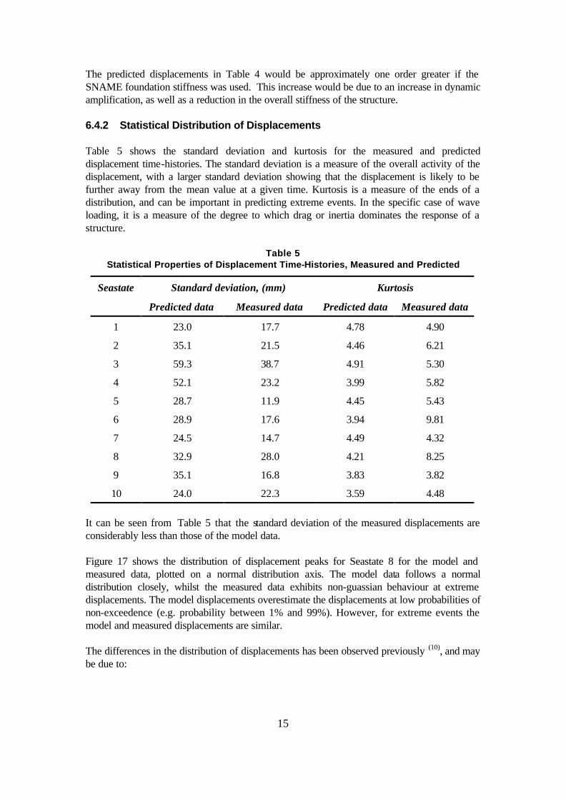
The predicted displacements in Table 4 would be approximately one order greater if the SNAME foundation stiffness was used. This increase would be due to an increase in dynamic amplification, as well as a reduction in the overall stiffness of the structure. 6.4.2 Statistical Distribution of Displacements Table 5 shows the standard deviation and kurtosis for the measured and predicted displacement time-histories. The standard deviation is a measure of the overall activity of the displacement, with a larger standard deviation showing that the displacement is likely to be further away from the mean value at a given time. Kurtosis is a measure of the ends of a distribution, and can be important in predicting extreme events. In the specific case of wave loading, it is a measure of the degree to which drag or inertia dominates the response of a structure.

Table 5 Statistical Properties of Displacement Time-Histories, Measured and Predicted

Standard deviation, (mm) Kurtosis Seastate

Predicted data Measured data Predicted data Measured data

1 23.0 17.7 4.78 4.90

2 35.1 21.5 4.46 6.21

3 59.3 38.7 4.91 5.30

4 52.1 23.2 3.99 5.82

5 28.7 11.9 4.45 5.43

6 28.9 17.6 3.94 9.81

7 24.5 14.7 4.49 4.32

8 32.9 28.0 4.21 8.25

9 35.1 16.8 3.83 3.82

10 24.0 22.3 3.59 4.48

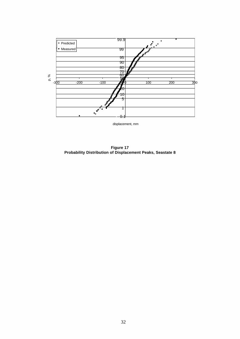
It can be seen from Table 5 that the standard deviation of the measured displacements are considerably less than those of the model data. Figure 17 shows the distribution of displacement peaks for Seastate 8 for the model and measured data, plotted on a normal distribution axis. The model data follows a normal distribution closely, whilst the measured data exhibits non-guassian behaviour at extreme displacements. The model displacements overestimate the displacements at low probabilities of non-exceedence (e.g. probability between 1% and 99%). However, for extreme events the model and measured displacements are similar. The differences in the distribution of displacements has been observed previously (10), and may be due to:

16

i. No wave spreading has been modelled, and hence all the wave energy in the model is applied in one plane. This, in turn, leads to greater displacement activity in that direction in the model compared to the actual structure.

ii. A difference in the distribution of wave heights in the measured and modelled data.

17

6.5 Maximum Foundation Loads Foundation loads during the storm simulations were calculated to determine if the foundations were being highly utilised. The maximum vertical, horizontal and rotational foundation load occurred during seastate 3. The following maximum foundation loads were determined: Maximum Moment 44120 kNm Maximum Horizontal Force 2820 kN Maximum Vertical Force (wave load only) 4892kN downwards

4448kN upwards The loads above represent less than 30% of the computed ultimate capacities.

18

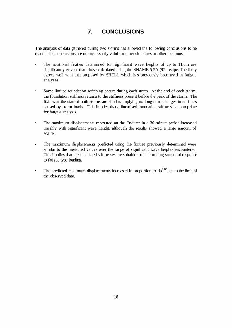
7. CONCLUSIONS The analysis of data gathered during two storms has allowed the following conclusions to be made. The conclusions are not necessarily valid for other structures or other locations. • The rotational fixities determined for significant wave heights of up to 11.6m are

significantly greater than those calculated using the SNAME 5-5A (97) recipe. The fixity agrees well with that proposed by SHELL which has previously been used in fatigue analyses.

• Some limited foundation softening occurs during each storm. At the end of each storm,

the foundation stiffness returns to the stiffness present before the peak of the storm. The fixities at the start of both storms are similar, implying no long-term changes in stiffness caused by storm loads. This implies that a linearised foundation stiffness is appropriate for fatigue analysis.

• The maximum displacements measured on the Endurer in a 30-minute period increased

roughly with significant wave height, although the results showed a large amount of scatter.

• The maximum displacements predicted using the fixities previously determined were

similar to the measured values over the range of significant wave heights encountered. This implies that the calculated stiffnesses are suitable for determining structural response to fatigue type loading.

• The predicted maximum displacements increased in proportion to Hs1.85, up to the limit of

the observed data.

19

8. REFERENCES (1) “Site Specific Assessment of Mobile Jack-Up Units, TR 5-5A”, Society of Naval

Architects and Marine Engineers (SNAME), Jersey City, 1997.

(2) Nelson J, Smith P, Hoyle M Stonor R and Versavel T (2000), “Jack-up Response Measurements and the Underprediction of Spud-can Fixity by SNAME 5-5A”, Offshore Technology Conference 12074.

(3) Hambly E, Imm G and Stahl B (1990), “Jack-Up Performance and Foundation Fixity Under Developing Storm Conditions”, Offshore Technology Conference 6466.

(4) Hunt R (1999), “Jack-up and Jacket Relative Motions; Prediction and Measurement”, Jack-up Conference, City University.

(5) “Metocean Criteria for Design – Central North Sea Regional Study”, SHELL UK, EN/080 Rev 1

(6) SHELL calculation of foundation stiffness

(7) “Maersk Endurer Mobile Jack-Up Drilling Unit. Shearwater Site-Specific Assessment Studies”, Nobel Denton Report No. L17726/NDE/GAH 1997.

(8) Morandi A, Karunakaran D, Dixon A and Baerheim M (1998), “Comparison of Full-Scale Measurements and Time-Domain Irregular Sea Analysis for a Large Deepwater Jack-Up”, Offshore Technology Conference.

(9) “Validation of Wave Response Analysis for Jack-Up Rigs”, HSE Offshore Technology Report 2000/094.

(10) Brekke J, Cambell R, Lamb W and Murff J (1990), “Calibration of a Jackup Analysis Procedure Using Field Measurements from a North Sea Jackup”, Offshore Technology Conference 6465.

20

Figure 1 General Configuration of Shearwater Platforms

21

Figure 2 Site Map

22

MeasuredSeastates

Jack-upResponse Data

Analysis:Plot of Fixity v.Natural Period

Inferred FixityAnalysis

Predicted Fixity(e.g. SNAME,Shell method)

Compare Fixities

CompareDeflections

PredictedDeflectionResponse

Naturalperiod

Deflections

Figure 3 Methodology flowchart

23

Figure 4

Significant wave heights measured in Storms A and B

Wave data at Auk, Kittiwake & Gannet for December 26th - 27th 1998

0

2

4

6

8

10

12

12/2

6/98

18:

00

12/2

7/98

6:0

0

12/2

7/98

18:

00

Sig

nific

ant W

ave

heig

ht (m

)

Auk

Kitt

Gann

Wave Data at Auk, Kittiwake & Gannet for February 2nd - 7th 1999

0

2

4

6

8

10

12

2/2/

99 1

8:00

2/3/

99 6

:00

2/3/

99 1

8:00

2/4/

99 6

:00

2/4/

99 1

8:00

2/5/

99 6

:00

2/5/

99 1

8:00

2/6/

99 6

:00

2/6/

99 1

8:00

2/7/

99 6

:00

2/7/

99 1

8:00

Sig

nific

ant W

ave

heig

ht (

m)

Auk

Kitt

Gann

24

Figure 5

Displacement Spectral density plot for Seastate 1

0

0.001

0.002

0.003

0.004

0.005

0.006

0.007

0 0.1 0.2 0.3 0.4 0.5

frequency, Hz

spec

tral

den

sity

, m2/

Hz

wave energy peak

response peak

25

Figure 6 SACS Model of Endurer

26

0.0

2.0

4.0

6.0

8.0

10.0

12.0

14.0

1.00E+06 1.00E+07 1.00E+08 1.00E+09

K rot, kNm/rad

Per

iod

, s

Sway

Surge

pinned

fixed

Figure 7

Variation of Predicted Natural Period with Foundation Rotational Fixity

max displacement, mm

1

5040

30

20

10

5

60

70

80

90

95

99

prob

abili

ty o

f non

-exc

eede

nce,

%

110 120 130 140 150 160 170 180 190 200

Figure 8

Distribution of maximum displacements for 100 random wave simulations

27

SEASTATE 1

0

50

100

150

200

250

300

350

400

450

0 0.05 0.1 0.15 0.2 0.25 0.3

f, Hz

Sn

n(f

), m2 /H

z

SACS Generated

theoretical, frommeasured data

SEASTATE 3

0

50

100

150

200

250

300

350

400

450

0 0.05 0.1 0.15 0.2 0.25 0.3

f, Hz

Sn

n(f

), m2

/Hz

SACS Generated

theoretical, frommeasured data

SEASTATE 2

0

50

100

150

200

250

300

350

400

450

0 0.05 0.1 0.15 0.2 0.25 0.3

f, Hz

Sn

n(f

), m2

/Hz

SACS Generated

theoretical, frommeasured data

SEASTATE 4

0

50

100

150

200

250

300

350

400

450

0 0.05 0.1 0.15 0.2 0.25 0.3

f, Hz

Sn

n(f

), m2 /H

z

SACS Generated

theoretical, frommeasured data

SEASTATE 5

0

50

100

150

200

250

300

350

400

450

0 0.05 0.1 0.15 0.2 0.25 0.3

f, Hz

Sn

n(f

), m2 /H

z

SACS Generated

theoretical, frommeasured data

SEASTATE 6

0

50

100

150

200

250

300

350

400

450

0 0.05 0.1 0.15 0.2 0.25 0.3

f, Hz

Sn

n(f

), m2

/Hz

SACS Generated

theoretical, frommeasured data

SEASTATE 7

0

50

100

150

200

250

300

350

400

450

0 0.05 0.1 0.15 0.2 0.25 0.3

f, Hz

Sn

n(f

), m2 /H

z

SACS Generated

theoretical, frommeasured data

SEASTATE 8

0

50

100

150

200

250

300

350

400

450

0 0.05 0.1 0.15 0.2 0.25 0.3

f, Hz

Sn

n(f

), m2 /H

z

SACS Generated

theoretical, frommeasured data

SEASTATE 9

0

50

100

150

200

250

300

350

400

450

0 0.05 0.1 0.15 0.2 0.25 0.3

f, Hz

Sn

n(f

), m

2 /Hz

SACS Generated

theoretical, frommeasured data

SEASTATE 10

0

50

100

150

200

250

300

350

400

450

0 0.05 0.1 0.15 0.2 0.25 0.3

f, Hz

Sn

n(f

), m

2 /Hz

SACS Generated

theoretical, frommeasured data

Figure 9

Comparison of SACS generated and Measured Wave Spectra

28

0

2

4

6

8

10

12

14

0 2 4 6 8 10 12

Seastate snapshot

Hs,

m

5.1

5.3

5.5

5.7

5.9

6.1

6.3

6.5

Tn, s

ec

Hs, Storm A Hs, Storm B

Tp, Storm A Tp, Storm B

Storm A Storm B

Figure 10

Variation of Natural Period during Storms A and B

4.00E+00

5.00E+07

1.00E+08

1.50E+08

2.00E+08

2.50E+08

3.00E+08

0 2 4 6 8 10 12

Seastate snapshot

Kro

t, k

Nm

/rad

Tp, Storm A Tp, Storm B

Storm A Storm B

Figure 11

Variation in Inferred Rotational Fixity during Storms A and B

29

0

0.2

0.4

0.6

0.8

1

0 2 4 6 8 10 12

Seastate

dyn

amic

fixi

ty

Storm A

Storm B

Storm A Storm B

Figure 12 Variation in Dynamic Fixity during Storms A and B

1.0E+06

1.0E+07

1.0E+08

1.0E+09

6 7 8 9 10 11 12

Hs, m

Kro

t, kN

m/r

ad

Storm AStorm B

SNAME "Extreme" stiffness

Shell "Fatigue" stiffness

Figure 13 Variation in Rotational Fixity with Significant Wave Height

30

Figure 14

Typical model displacement time-history, Seastate 8

-200

0

200

0 100 200 300 400 500 600 700 800 900

time, sec

disp

, mm

-200

0

200

900 1000 1100 1200 1300 1400 1500 1600 1700 1800

time, sec

disp

, mm

31

Figure 15

Spectral density of displacement, Seastate 8

0

50

100

150

200

250

300

350

400

0 2 4 6 8 10 12 14 16

Hs, m

max

. dis

pla

cem

ent,

mm

Measured data

Predicted displacements

Figure 1

Measured and Predicted Maximum Displacements

0

0.01

0.02

0.03

0.04

0.05

0.06

0 0.05 0.1 0.15 0.2 0.25 0.3 0.35

frequency, Hz

Sp

ectr

al d

enis

ty, m

2/H

z

wave energy peak

response peak

-3.1

0

3.1

-300 -200 -100 0 100 200 300

displacement, mm

p, %

Predicted

Measured

80

50

99

5

20

70

99.9

3

95

10

90

60

0.1

1

40

Figure 17 Probability Distribution of Displacement Peaks, Seastate 8

32

33

Printed and published by the Health and Safety ExecutiveC0.35 3/02

OTO 2001/035

£20.00 9 780717 622986

ISBN 0-7176-2298-3