On the Optimality of Spectral Compression of Mesh Data

On the Optimality of Spectral Compression of Mesh Data

MIRELA BEN-CHEN and CRAIG GOTSMANTechnion—Israel Institute of Technology

Spectral compression of the geometry of triangle meshes achieves good results in practice, but there has been little or no theoreticalsupport for the optimality of this compression. We show that, for certain classes of geometric mesh models, spectral decompositionusing the eigenvectors of the symmetric Laplacian of the connectivity graph is equivalent to principal component analysis onthat class, when equipped with a natural probability distribution. Our proof treats connected one-and two-dimensional mesheswith fixed convex boundaries, and is based on an asymptotic approximation of the probability distribution in the two-dimensionalcase. The key component of the proof is that the Laplacian is identical, up to a constant factor, to the inverse covariance matrixof the distribution of valid mesh geometries. Hence, spectral compression is optimal, in the mean square error sense, for theseclasses of meshes under some natural assumptions on their distribution.

Categories and Subject Descriptors: I.3.5 [Computer Graphics]: Computational Geometry and Object Modeling; E.4 [Codingand Information Theory]

General Terms: Theory

Additional Key Words and Phrases: Triangle mesh, spectral decomposition, Laplacian

1. INTRODUCTION

Triangle meshes are a popular way of representing 3D shape models. As the size and detail of themodels grow, compression of the models becomes more and more important. The size of the mesh datafiles can be reduced by compressing either the geometry or the connectivity of the mesh, or both.

There has been much research into both geometry and connectivity coding. Most connectivity codingschemes, for example the Edgebreaker [Rossignac 1999] and the TG methods [Touma and Gotsman1998], are based on traversing the mesh and generating code symbols representing new vertices or facesas they are traversed. The quality of the compression results from the entropy of the symbol sequence.

Typical geometry coding schemes are based on the fact that the coordinates of a mesh are not in-dependent, and specifically, the coordinates of neighboring vertices are highly correlated, especiallyin smooth meshes. This correlation can be exploited by using “prediction rules”—the coordinates of avertex are predicted from the coordinates of neighboring vertices, and only the prediction error vectoris coded [Taubin and Rossignac 1998; Touma and Gotsman 1998]. The better the prediction rule is, thesmaller the errors are, and the smaller the entropy of the code will be.

Spectral compression of mesh geometry [Karni and Gotsman 2000] also exploits the correlation amongneighboring vertices, and implicitly applies a prediction rule that every vertex is the simple average

This work was partially supported by the Israel Ministry of Science Grant 01-01-01509, the German-Israel Fund (GIF)Grant I-627-45.6/1999, European FP5 RTN Grant HPRN-CT-1999-00117 (MINGLE), and European FP6 NoE Grant 506766(AIM@SHAPE).Authors’ addresses: Department of Computer Science, Technion-Israel Institute of Technology, Haifa 32000 Israel; email:{mirela,gotsman}@cs.technion.ac.il.Permission to make digital or hard copies of part or all of this work for personal or classroom use is granted without fee providedthat copies are not made or distributed for profit or direct commercial advantage and that copies show this notice on the firstpage or initial screen of a display along with the full citation. Copyrights for components of this work owned by others than ACMmust be honored. Abstracting with credit is permitted. To copy otherwise, to republish, to post on servers, to redistribute to lists,or to use any component of this work in other works requires prior specific permission and/or a fee. Permissions may be requestedfrom Publications Dept., ACM, Inc., 1515 Broadway, New York, NY 10036 USA, fax: +1 (212) 869-0481, or [email protected]© 2005 ACM 0730-0301/05/0100-0060 $5.00

ACM Transactions on Graphics, Vol. 24, No. 1, January 2005, Pages 60–80.

The Optimality of Spectral Compression of Mesh Data • 61

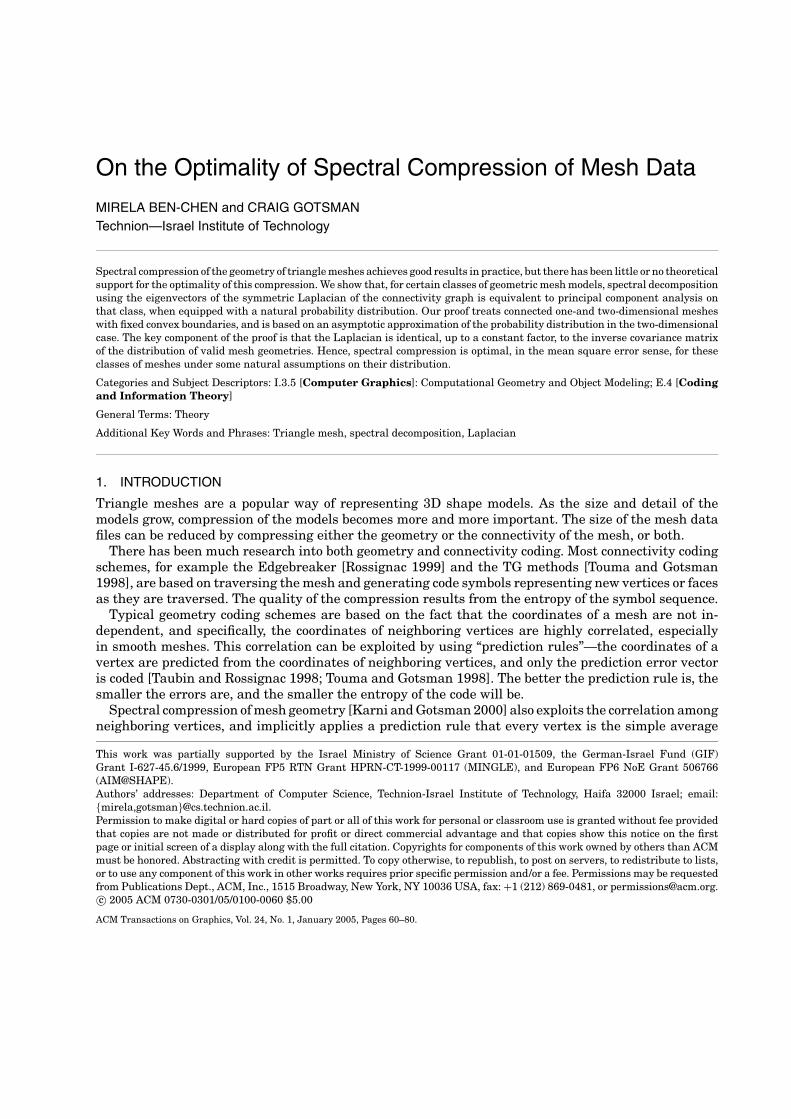
Fig. 1. A simple irregular mesh and its symmetric Laplacian.

of all its immediate neighbors. Inspired by traditional signal coding, spectral decomposition has beenproposed for lossy transform coding of the geometry of a mesh with irregular connectivity. Althoughthe method yields good results in practice, there is little theoretical support for the optimality of suchcompression.

Motivated by the optimality of the Discrete Cosine Transform (DCT) in signal processing [Rao andYip 1990], we wish to prove a similar result for spectral compression, namely, that it is optimal forcertain classes of irregular meshes. Our proof covers connected meshes in one and two dimensionswith fixed convex boundaries. The proof for the two-dimensional case is based on an asymptotic normalapproximation.

1.1 Previous Work

Let G be a graph, G = (V , E), where V is the vertex set, and E the edge set. A k-dimensional meshM is M = (G, R), R = (X (1), X (2), . . . , X (k)), where X (i) is a real vector of the i-th dimension coordinatevalues of the mesh vertices. We sometimes refer to E as the connectivity and to R as the geometry ofthe mesh M .

Given a mesh M = (G, R), G = (V , E), the symmetric Laplacian of M is the matrix L:

Li, j =

di i = j0 (i, j ) /∈ E−1 (i, j ) ∈ E

where di is the number of neighbors (valence) of the i-th vertex. A mesh with constant valences is calleda regular mesh; otherwise, it is called an irregular mesh. See Figure 1 for an example of an irregularmesh, and its corresponding Laplacian.

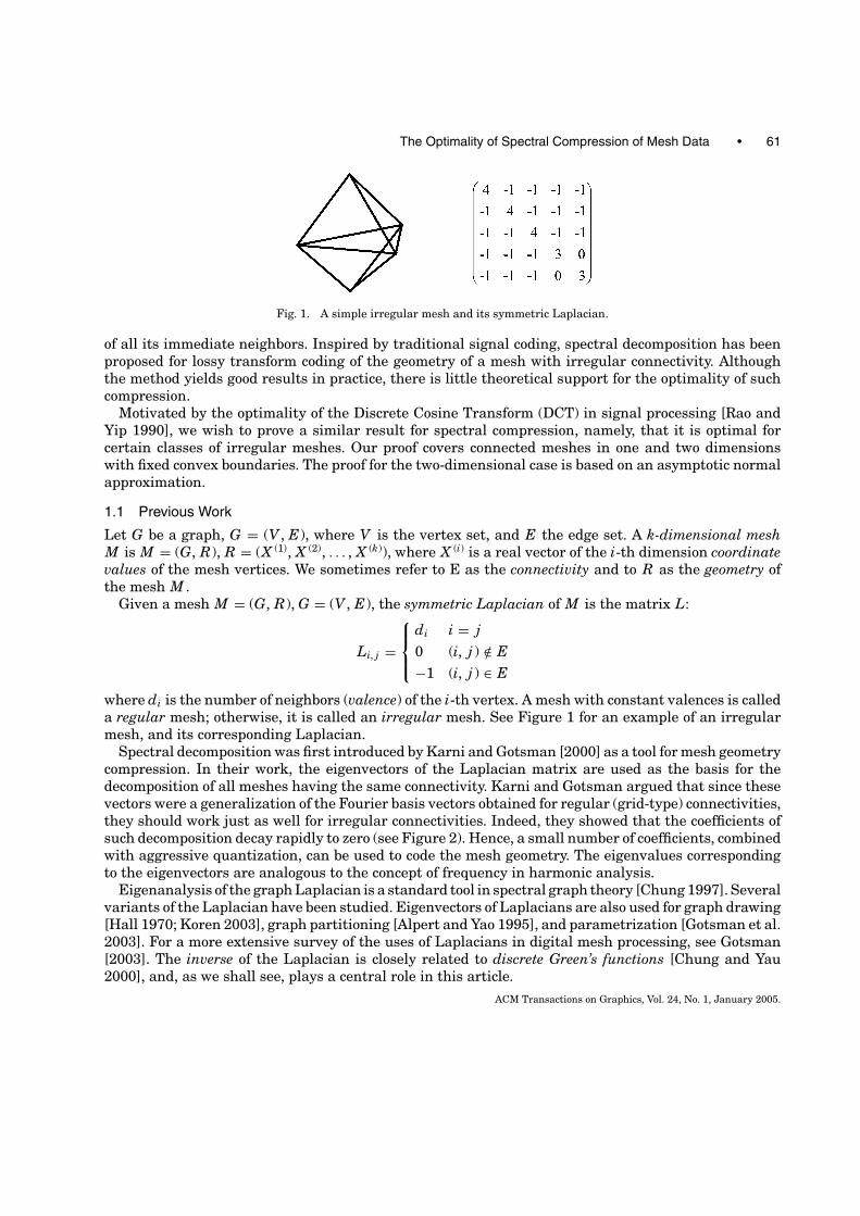
Spectral decomposition was first introduced by Karni and Gotsman [2000] as a tool for mesh geometrycompression. In their work, the eigenvectors of the Laplacian matrix are used as the basis for thedecomposition of all meshes having the same connectivity. Karni and Gotsman argued that since thesevectors were a generalization of the Fourier basis vectors obtained for regular (grid-type) connectivities,they should work just as well for irregular connectivities. Indeed, they showed that the coefficients ofsuch decomposition decay rapidly to zero (see Figure 2). Hence, a small number of coefficients, combinedwith aggressive quantization, can be used to code the mesh geometry. The eigenvalues correspondingto the eigenvectors are analogous to the concept of frequency in harmonic analysis.

Eigenanalysis of the graph Laplacian is a standard tool in spectral graph theory [Chung 1997]. Severalvariants of the Laplacian have been studied. Eigenvectors of Laplacians are also used for graph drawing[Hall 1970; Koren 2003], graph partitioning [Alpert and Yao 1995], and parametrization [Gotsman et al.2003]. For a more extensive survey of the uses of Laplacians in digital mesh processing, see Gotsman[2003]. The inverse of the Laplacian is closely related to discrete Green’s functions [Chung and Yau2000], and, as we shall see, plays a central role in this article.

ACM Transactions on Graphics, Vol. 24, No. 1, January 2005.

62 • M. Ben-Chen and C. Gotsman

Fig. 2. Spectral decomposition. (a) The horse model and (b, c, d) the spectral coefficients of its decomposition in the X , Y , andZ dimensions.

The rest of the article is organized as follows. Section 2 defines the terminology used throughout thearticle. Section 3 reviews the concept of principal component analysis, a key tool in our proofs, whichis the motivation for studying the eigenvectors of the covariance matrix. Sections 4 and 5 prove theoptimality result for the 1D and 2D cases, respectively. To conclude, Section 6 discusses our model andexplores future research directions.

2. DEFINITIONS

The decomposition of a vector X nx1, by the orthonormal basis of Rn : Unxn = {U1, . . . , Un}, is:

X =n∑

i=1

ciUi, (1)

where C ={ci} are the coefficients of the decomposition.The reconstruction of a vector X from its decomposition using the first k coefficients is:

X (U,k) =k∑

i=1

ciUi. (2)

Note that the order of the basis vectors is important, as only a prefix of them is used in the k-threconstruction.ACM Transactions on Graphics, Vol. 24, No. 1, January 2005.


Because of the orthonormality of U , the Parseval identity maintains that ‖c‖ = ‖X‖. A decompositionis useful when a small number of the coefficients contain a large portion of the norm (energy) of thevector. If this is the case, those coefficients alone may be used in the reconstruction, and the Euclideandistance between the reconstructed vector and the original X will be small. This is a useful feature forcompression applications.

For a specific vector X , the best basis will always be {X , 0, 0, . . . , 0}, since then all the energy is con-tained in the first coefficient. Hence, there is a meaningful answer to the question “what is the optimalbasis for decomposition” only if we consider an entire family of vectors (finite or infinite). In our context,the family will be all the geometries which are valid for a given mesh connectivity E. These geometrieswill be specified by imposing an appropriate probability distribution D, derived from E, on Rn.

If X is a random variable, we denote by Exp(X ) the expectation of X , by Var(X ) the variance of Xfor scalar X , and by Cov(X ) the covariance matrix of X for vector X .

Given a probability distribution D on Rn, we say that a vector basis U is an optimal basis for D, iffor any other basis W , and for every 1 ≤ k ≤ n:

Exp((

X − X (U,k))2) ≤ Exp

((X − X (W,k)

)2) (3)

where the expectation is taken over D. This is called optimality in the Mean Square Error (MSE) sense.

3. PRINCIPAL COMPONENT ANALYSIS

Approximation of random signals has been studied extensively in signal processing. A well-knownoptimality result, which we will rely on heavily, is related to the so-called Principal Component Analysis(PCA) procedure.

Assume a random vector X ∈ Rn, sampled from distribution D, having zero mean vector and co-variance matrix C. Denote by {�i|i = 1, . . , n} the eigenvectors of C, with corresponding eigenvalues{λi|i = 1, . . . , n}, ordered such that λ1 ≥ λ2 ≥ · · · ≥ λn. The matrix � is called the Principal ComponentAnalysis of X , sometimes known as the Karhunen-Loeve or Hotelling transform of X .

It is well known [Jolliffe 1986] that the PCA is optimal in the MSE sense, as defined in (3). Note that� does not depend on k—the number of vectors used for the reconstruction—so the optimal basis forreconstruction from k + 1 basis vectors contains the optimal basis for reconstruction from k vectors.

When the class of meshes is finite and given, containing T meshes, for example, an animation se-quence of a mesh with a fixed connectivity, the natural distribution is a uniform distribution on thisfinite set. In this case, the PCA of that class may be computed using the numerical Singular ValueDecomposition (SVD) procedure [Press et al. 1987] on a matrix of size 3n × T , consisting of T columns,where the i-th column contains the coordinate values of the i-th mesh in the sequence. This was proposedby Alexa and Muller [2000] for compressing animated meshes.

To compute the PCA of an infinite continuum of meshes with a given connectivity, where none ofthem is explicitly given, we must first make some assumptions about the distribution D of this family,and then compute the covariance matrix C of this distribution. We will do this, and then show thatC is essentially identical to the inverse of the mesh Laplacian matrix, up to a constant factor. Due tothis special relationship, both matrices have identical eigenvectors (in opposite order), from which ouroptimality theorem will follow.

4. 1D MESHES

Before we proceed, a note about the connection between the proof for one dimension, and the proof fortwo dimensions is in order. Basically, for both cases we prove the same theorem—that L = αC−1, forsome constant α. While for the one-dimensional case the theorem can be proved relatively easily, in twodimensions we resort to asymptotic approximations.



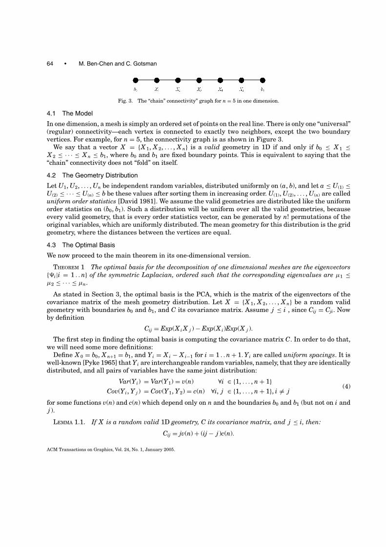
Fig. 3. The “chain” connectivity” graph for n = 5 in one dimension.

4.1 The Model

In one dimension, a mesh is simply an ordered set of points on the real line. There is only one “universal”(regular) connectivity—each vertex is connected to exactly two neighbors, except the two boundaryvertices. For example, for n = 5, the connectivity graph is as shown in Figure 3.

We say that a vector X = {X 1, X 2, . . . , X n} is a valid geometry in 1D if and only if b0 ≤ X 1 ≤X 2 ≤ · · · ≤ X n ≤ b1, where b0 and b1 are fixed boundary points. This is equivalent to saying that the“chain” connectivity does not “fold” on itself.

4.2 The Geometry Distribution

Let U1, U2, . . . , Un be independent random variables, distributed uniformly on (a, b), and let a ≤ U(1) ≤U(2) ≤ · · · ≤ U(n) ≤ b be these values after sorting them in increasing order. U(1), U(2), . . . , U(n) are calleduniform order statistics [David 1981]. We assume the valid geometries are distributed like the uniformorder statistics on (b0, b1). Such a distribution will be uniform over all the valid geometries, becauseevery valid geometry, that is every order statistics vector, can be generated by n! permutations of theoriginal variables, which are uniformly distributed. The mean geometry for this distribution is the gridgeometry, where the distances between the vertices are equal.

4.3 The Optimal Basis

We now proceed to the main theorem in its one-dimensional version.

THEOREM 1 The optimal basis for the decomposition of one dimensional meshes are the eigenvectors{�i|i = 1 . . n} of the symmetric Laplacian, ordered such that the corresponding eigenvalues are µ1 ≤µ2 ≤ · · · ≤ µn.

As stated in Section 3, the optimal basis is the PCA, which is the matrix of the eigenvectors of thecovariance matrix of the mesh geometry distribution. Let X = {X 1, X 2, . . . , X n} be a random validgeometry with boundaries b0 and b1, and C its covariance matrix. Assume j ≤ i , since Cij = Cji. Nowby definition

Cij = Exp(X i X j ) − Exp(X i)Exp(X j ).

The first step in finding the optimal basis is computing the covariance matrix C. In order to do that,we will need some more definitions:

Define X 0 = b0, X n+1 = b1, and Yi = X i − X i−1 for i = 1 . . n + 1. Yi are called uniform spacings. It iswell-known [Pyke 1965] that Yi are interchangeable random variables, namely, that they are identicallydistributed, and all pairs of variables have the same joint distribution:

Var(Yi) = Var(Y1) = v(n) ∀i ∈ {1, . . . , n + 1}Cov(Yi, Y j ) = Cov(Y1, Y2) = c(n) ∀i, j ∈ {1, . . . , n + 1}, i �= j

(4)

for some functions v(n) and c(n) which depend only on n and the boundaries b0 and b1 (but not on i andj ).

LEMMA 1.1. If X is a random valid 1D geometry, C its covariance matrix, and j ≤ i, then:

Cij = jv(n) + (ij − j )c(n).



PROOF. From the definition of Yi we have that:

X i = b0 +i∑

k=1

Yk . (5)

Then, for j ≤ i, by substituting (5) in the covariance definition, and since the Yi are interchangeableas defined in (4), we have:

Cij = Exp(X i X j ) − Exp(X i) Exp(X j ) =i∑

k=1

j∑r=1

[Exp(YkYr ) − Exp(Yk) Exp(Yr )]

=j∑

r=1

[Exp

(Y 2

r

) − Exp(Yr )2] +i∑

k=1

j∑r=1r �=k

[Exp(YkYr ) − Exp(Yk) Exp(Yr )] (6)

=j∑

r=1

var(Y1) +i∑

k=1

j∑r=1r �=k

cov(Y1, Y2) = jv(n) + (ij − j )c(n).

We will now relate the variance and covariance of the uniform spacings, which will allow us to simplifythe expression in (6).

LEMMA 1.2. If v(n) and c(n) are the variance and covariance, respectively, of uniform spacings asdefined in (4), then:

c(n) = −1n

v(n).

PROOF. Consider the following expression:

Exp

(

n+1∑i=1

Yi

)2 −

[Exp

(n+1∑i=1

Yi

)]2

.

On the one hand, developing the expression, by expanding the sums and using the linearity of theexpectation, yields:

Exp

(

n+1∑i=1

Yi

)2 −

[Exp

(n+1∑i=1

Yi

)]2

=n+1∑i=1

n+1∑j=1

Exp(YiY j ) −n+1∑i=1

n+1∑j=1

Exp(Yi) Exp(Y j )

=n+1∑i=1

n+1∑j=1

[Exp(YiY j ) − Exp(Yi) Exp(Y j )]

=n+1∑j=1

[Exp

(Y 2

j

) − Exp(Y j )2]

+n+1∑i=1

n+1∑j=1i �= j

[Exp(YiY j ) − Exp(Yi) Exp(Y j )] (7)

=n+1∑j=1

var(Y1) +n+1∑i=1

n+1∑j=1i �= j

cov(Y1, Y2)

= (n + 1)v(n) + n(n + 1)c(n).ACM Transactions on Graphics, Vol. 24, No. 1, January 2005.


On the other hand, since the sum of the Yi is the constant (b1 − b0), we have:

Exp

(n+1∑i=1

Yi

)2 −

[Exp

(n+1∑i=1

Yi

)]2

= (b1 − b0)2 − (b1 − b0)2 = 0. (8)

Comparing (7) and (8), we have:

(n + 1)v(n) + n(n + 1)c(n) = 0 (9)

c(n) = −1n

v(n)

Note that the covariance of two spacings is always negative. Intuitively, this is because one spacingmay grow only at the expense of the other spacings, since their sum is constant.

By using the two previous lemmas, we can now simplify the expression of the covariance, by substi-tuting (9) in (6), to get:

Cij = j (n − i + 1)v(n)

nfor every 1 ≤ j ≤ i ≤ n.

So, the covariance matrix C is

Cij ={

j (n − i + 1) v(n)n 1 ≤ j ≤ i ≤ n

Cji 1 ≤ i < j ≤ n(10)

Now let us examine the matrix product L · C. The valence di of all the (interior) vertices is 2, sinceevery vertex has exactly two neighbors. Hence, the Laplacian is the n × n matrix:

L =

2 −1 0 · · · 0

−1 2 −1. . .

...

0. . . 0

.... . . −1 2 −1

0 · · · 0 −1 2

(n×n)

where n is the number of interior vertices.Note that the Laplacian has entries only for the interior vertices, so the first and last rows do not sum

to zero, since they belong to vertices neighboring on the boundaries. This property makes the Laplacianinvertible.

By substituting (10) in the product L·C, it is easy to see that:

(L · C)i, j ={

k(n) i = j0 i �= j ,

where k(n) depends only on n, and is

k(n) = v(n)(n + 1)n

,

which implies that

L · C = k(n)IACM Transactions on Graphics, Vol. 24, No. 1, January 2005.


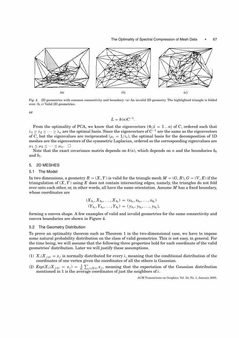
Fig. 4. 2D geometries with common connectivity and boundary: (a) An invalid 2D geometry. The highlighted triangle is foldedover. (b, c) Valid 2D geometries.

or

L = k(n)C−1.

From the optimality of PCA, we know that the eigenvectors {�i|i = 1 . . n} of C, ordered such thatλ1 ≥ λ2 ≥ · · · ≥ λn are the optimal basis. Since the eigenvectors of C−1 are the same as the eigenvectorsof C, but the eigenvalues are reciprocated (µi = 1/λi), the optimal basis for the decomposition of 1Dmeshes are the eigenvectors of the symmetric Laplacian, ordered so the corresponding eigenvalues areµ1 ≤ µ2 ≤ · · · ≤ µn.

Note that the exact covariance matrix depends on k(n), which depends on n and the boundaries b0and b1.

5. 2D MESHES

5.1 The Model

In two dimensions, a geometry R = (X , Y ) is valid for the triangle mesh M = (G, R), G = (V , E) if thetriangulation of (X , Y ) using E does not contain intersecting edges, namely, the triangles do not foldover onto each other, or, in other words, all have the same orientation. Assume M has a fixed boundary,whose coordinates are

(X b1 , X b2 , . . . , X bk ) = (xb1 , xb2 , . . . , xbk )(Yb1 , Yb2 , . . . , Ybk ) = ( yb1 , yb2 , . . . , ybk ),

forming a convex shape. A few examples of valid and invalid geometries for the same connectivity andconvex boundaries are shown in Figure 4.

5.2 The Geometry Distribution

To prove an optimality theorem such as Theorem 1 in the two-dimensional case, we have to imposesome natural probability distribution on the class of valid geometries. This is not easy, in general. Forthe time being, we will assume that the following three properties hold for each coordinate of the validgeometries’ distribution. Later we will justify these assumptions.

(1) X i|X j �=i = x j is normally distributed for every i, meaning that the conditional distribution of thecoordinates of one vertex given the coordinates of all the others is Gaussian.

(2) Exp(X i|X j �=i = x j ) = 1di

∑j∈N (i) x j , meaning that the expectation of the Gaussian distribution

mentioned in 1 is the average coordinates of just the neighbors of i.ACM Transactions on Graphics, Vol. 24, No. 1, January 2005.


(3) Cov(X i, X j | X k = xk , k �= i, j , (i, j ) �∈ E) = 0, meaning that the covariance of the coordinates of everytwo vertices i, j which are not neighbors, conditioned on the coordinates of all other vertices, is zero.

From now on, we will only refer to the X dimension, but all the theorems hold for the Y dimensiontoo.

5.3 The Optimal Basis

The 2D version of our optimality theorem is:

THEOREM 2. If the distribution of valid geometries of 2D meshes has the properties defined inSection 5.2, then the optimal basis for the decomposition of 2D meshes with connectivity graph G =(V , E) are the eigenvectors {�i|i = 1 . . n} of the symmetric Laplacian of G, ordered such that the corre-sponding eigenvalues are µ1 ≤ µ2 ≤ · · · ≤ µn.

We first show that if the distribution of valid geometries has the first two properties described inSection 5.2, then it is multivariate normal. Note that just normal conditionals do not necessarily implymultivariate normality. However, the following Lemma characterizes the multivariate normal distri-bution via its conditionals:

LEMMA 2.1. (ARNOLD ET AL. 1999). Let X = {X 1, X 2, . . . , X n} be a random vector. If:

(1) X i|X j �=i = x j is normally distributed for every i, and(2) Exp(X i|X j = x j ) is linear in x j and not constant, for every i,

then X has a multivariate normal distribution.

It is easy to see that the conditions of the lemma are satisfied if we assume the distribution of validgeometries has the first two properties described in Section 5.2. The first condition of the lemma isidentical to the first property described in Section 5.2. The second condition is implied by the secondproperty—if the conditional expectation of a vertex is the average of its neighbors, then it is linear in x j .In addition, since the mesh is connected, and there are no isolated vertices, the conditional expectationcannot be a constant with respect to the x j . Thus, the second condition of Lemma 2.1 also holds. Sinceboth the conditions of Lemma 2.1 hold, we conclude that the distribution of valid geometries (assumingSection 5.2) is multivariate normal.

Now that we have characterized the distribution of the geometries, we proceed to compute the covari-ance matrix, which is the key for proving optimality. The next two lemmas characterize the structureof K —the inverse of the covariance matrix. Combined, they show that K is essentially identical to themesh Laplacian.

LEMMA 2.2. Let C be the covariance matrix of the X component of a random valid geometry R =(X , Y ) of a mesh M = (G, R), G = (V , E). Let K = C−1. Then for every (i, j ), such that i �= j , and(i, j ) /∈ E, Ki, j = 0.

PROOF. We need the following lemma which describes a few known properties of the inverse covari-ance matrix K of a multinormal distribution:

LEMMA 2.3 (LAURITZEN 1996). Let X be a multivariate normal random variable X ∼ N (µ, �), andlet K = �−1. Then:

(1) Kij = −Cov(X i, X j |X k �=i, j = xk)(KiiKjj − K 2ij).

(2) Exp(X i|X j �=i = x j ) = Exp(X i) + ∑j �=i βij(x j − Exp(X j )), βij = − Kij

Kii.



Part 1 of Lemma 2.3, and the vanishing conditional covariance described in the third property ofSection 5.2 imply that if i and j are not neighbors, then Kij = 0.

For the entries of K corresponding to the vertices and edges of the connectivity graph, we need thefollowing Lemma.

LEMMA 2.4. Let C be the covariance matrix of the X component of a random valid geometry R = (X , Y )of a mesh M = (G, R), G = (V , E). Let K = C−1. Then, there exists a constant α, such that:

(1) For every (i, j ) ∈ E, Kij = −α

(2) For every i ∈ V , Kii = αdi

PROOF. From part 2 of Lemma 2.3, we know that

Exp(X i|X j �=i = x j ) = Exp(X i) +∑j �=i

βij (x j − Exp(X j )).

On the other hand, we assumed in the second property of Section 5.2 that

Exp(X i|X j �=i = x j ) = 1di

∑j∈N (i)

x j .

Since the linear coefficients of x j must be equal in both expressions, we have

βij = − Kij

Kii= 1

di. (11)

C is a covariance matrix, so both C and K are symmetric, hence

Kii

di= −Kij = −Kji = Kjj

d j(12)

for every (i, j ) ∈ E.Consider the diagonal of K . It is easy to see that if the mesh is connected, all the values Kii/di must

equal a constant α that does not depend on i: Define K11/d1 = α. From (12) we have that for all theneighbors j ∈ N (1), Kjj/d j = K11/d1 = α. The same can be done inductively for the neighbors of j andso on. Finally, since the mesh is connected, every vertex i has a path to the first vertex, so it must holdthat:

Kii

di= α (13)

for every i ∈ V . Substituting (13) in (12) implies

Kij = −α (14)

for every (i, j ) ∈ E

Combining Lemmas 2.2 and 2.4, we conclude:Let C be the covariance matrix of the X component of a random valid geometry R = (X , Y ) of a mesh

M = (G, R), G = (V , E). Let K = C−1. Then K is:

Kij =

−α (i, j ) ∈ Eαdi i = j0 otherwise



Returning to the definition of the symmetric Laplacian in Section 1.1, we see that:

C−1 = K = αL,

where α is a constant that depends on n alone.As in the one-dimensional case, this concludes the proof of Theorem 2.

Note that the exact values of the covariance matrix depend on α, which depends on the fixed boundaryvalues.

Our theorem makes some powerful assumptions on the distribution of valid 2D geometries. We willnow show why it is reasonable to make such assumptions, by describing a natural model for generatingvalid 2D geometries, which turns out to have a distribution with the required properties.

Following Tutte [1963], Floater [1997] proved that a 2D geometry with a convex boundary is valid ifand only if each vertex is a convex combination of its neighbors. This implies that a geometry (X , Y )with a convex boundary (Bx , By ) is valid, if and only if there exists a matrix W such that

X = WX + Bx ,

Y = WY + BY (15)

where Bx and By are

Bxi ={

xi i ∈ {b1, . . . , bk}0 otherwise

Byi ={

yi i ∈ {b1, . . . , bk}0 otherwise

and W is

Wij ={

wij (i, j ) ∈ E, i /∈ {b1, . . . , bk}0 otherwise

.

The weights wij are positive and normalized:n∑

i=1

Wij = 1 i /∈ {b1, . . . , bk}.

We will call W a barycentric coordinates matrix.This characterization of valid 2D meshes yields a convenient way to define a probability distribution

on them. Instead of specifying the distribution of the valid geometries X (which seems to be quite diffi-cult), we specify the distribution of the barycentric coordinates matrices. We assume that the barycentriccoordinates matrices are distributed as follows:

For each interior vertex i, with valence di, let

wij = Dij = Ui

( j+1) − Ui( j ), (16)

where Ui( j ) are di − 1 order statistics over (0, 1), with Ui

(0) = 0, and Uid (i) = 1. Di

j are known as uniformspacings [Pyke 1965]. This guarantees that the nonzero Wij are indeed positive and all the internalvertices’ rows sum to one.

Note that such a distribution is not guaranteed to generate a uniform distribution of valid geometries.Since barycentric coordinates are not unique, that is, more than one set of barycentric coordinates cangenerate the same geometry, the use of barycentric coordinates may introduce a bias which will prefercertain valid geometries over others.

We now address the following question: If the barycentric coordinates matrices W are distributed asin (16), how are the geometries distributed? Given the matrix W and the boundary B, the geometry XACM Transactions on Graphics, Vol. 24, No. 1, January 2005.


can be expressed as

X = (I − W )−1 B,

where I is the identity matrix.

LEMMA 2.5. Let X be the x coordinate of a random valid geometry, whose barycentric coordinates aredistributed as in (16). Then the distribution of X has the following properties:

(1) The limit distribution of X i|X j �=i = x j as di → ∞ is normal for every i,

(2) Exp(X i|X j �=i = x j ) = 1di

∑j∈N (i) x j ,

(3) Cov(X i, X j |X k = xk , k �= i, j ) = 0 for every two vertices i, j which are not neighbors.

PROOF. From the definition of X and W in (15) and (16), respectively, it is easy to see that theconditioned variables (X i|X j = x j ) are

(X i|X j = x j ) =∑

j∈N (i)

Dij x j , (17)

where Dij are uniform spacings, N (i) is the set of neighbors of the i-th vertex, and the x j are constants.

The central limit theorem for functions of uniform spacings [Pyke 1965] implies that for vertices withlarge valence:

(X i|X j = x j ) ∼ Normal(µi, σ 2

i

)(18)

where Normal is the Gaussian distribution. This proves the first part of the Lemma.Since uniform spacings are interchangeable random variables which sum to unity:

di∑j=1

Dij = 1 ∀i

it follows that

Exp(Di

j

) = Exp(Di

1

) = 1di

∀ j . (19)

Substituting the expectation of the spacings (19), in (17), we obtain

µi = Exp(X i|X j = x j ) = Exp

( ∑j∈N (i)

Dij x j

)=

∑j∈N (i)

Exp(Di

j

)x j = 1

di

∑j∈N (i)

x j . (20)

Note that the x j are constants, since they are conditioned upon, so Exp(Dij x j ) = Exp(Di

j )x j .This proves the second part of the Lemma.Let i, j be two nonadjacent vertices. Consider the covariance of X i and X j conditioned on the rest ofthe vertices:

Cov(X i, X j |X k = xk , k �= i, j

) = Exp(X i X j |X k = xk) − Exp(X i|X k = xk)Exp(X j |X k = xk)

= Exp

( ∑r∈N (i)

Dir xr

∑m∈N ( j )

D jmxm

)− Exp

( ∑r∈N (i)

Dir xr

)Exp

( ∑m∈N ( j )

D jmxm

)

=∑

r∈N (i)

∑m∈N ( j )

Exp(Di

r xr D jmxm

)− ∑r∈N (i)

∑m∈N ( j )

Exp(Di

r xr)Exp

(D j

mxm).



Since i and j are not neighbors, Dir and D j

m are disjoint sets of independent uniform spacings, whichimplies that:

Exp(Di

r xr D jmxm

) = Exp(Di

r xr)

Exp(D j

mxm)

(21)

and thus,

Cov(X i, X j |X k = xk , k �= i, j ) = 0 (22)

for every nonadjacent i and j .This proves the third part of the Lemma and concludes its proof.

We now have a model for generating valid 2D meshes, which yields a distribution that has the prop-erties required in Section 5.2, with just one problem—the first property of Section 5.2 requires a normalconditional distribution, and all we have is a normal limit distribution as d → ∞. Central limit theo-rems with asymptotic parameter d → ∞ give very good approximations already for modest values of d .Here the asymptotic parameter is the valence, which is 6, on the average. The following experimentalresults show that it seems to be large enough for the normal approximation to be reasonable.

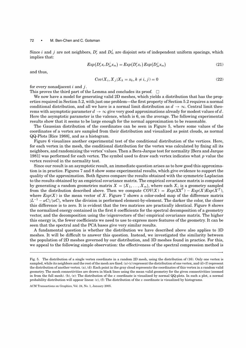
The Gaussian distribution of the coordinates can be seen in Figure 5, where some values of thecoordinates of a vertex are sampled from their distribution and visualized as point clouds, as normalQQ-Plots [Rice 1988], and as a histogram.

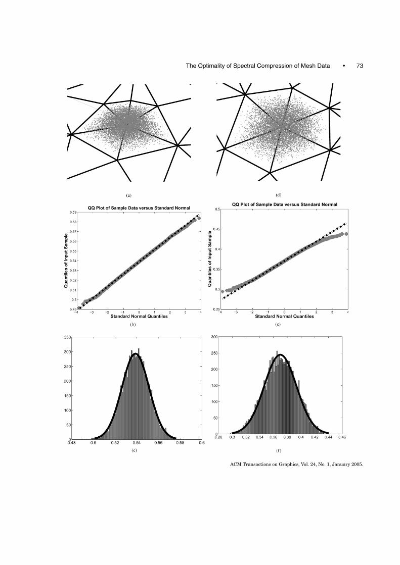
Figure 6 visualizes another experimental test of the conditional distribution of the vertices. Here,for each vertex in the mesh, the conditional distribution for the vertex was calculated by fixing all itsneighbors, and randomizing the vertex’ values. Then a Bera-Jarque test for normality [Bera and Jarque1981] was performed for each vertex. The symbol used to draw each vertex indicates what p value thevertex received in the normality test.

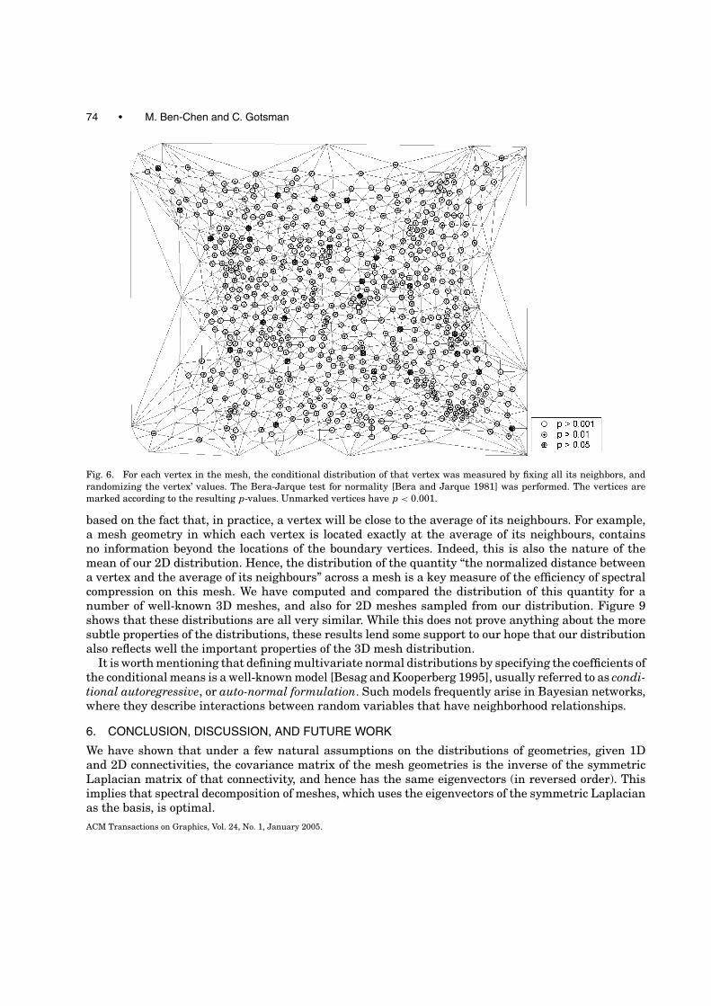
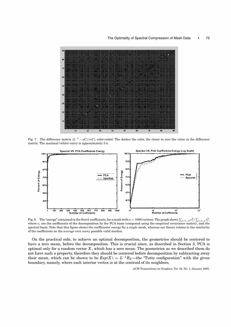
Since our result is an asymptotic result, an immediate question arises as to how good this approxima-tion is in practice. Figures 7 and 8 show some experimental results, which give evidence to support thequality of the approximation. Both figures compare the results obtained with the symmetric Laplacianto the results obtained by an empirical covariance matrix. The empirical covariance matrix is computedby generating a random geometries matrix X = {X 1, . . . , X m}, where each X i is a geometry sampledfrom the distribution described above. Then we compute COV(X ) = Exp(XXT ) − Exp(X )Exp(X T ),where Exp(X ) is the mean vector of X . Figure 7 shows a color-coded map of the difference matrix|L−1 − αC|/|αC|, where the division is performed element-by-element. The darker the color, the closerthis difference is to zero. It is evident that the two matrices are practically identical. Figure 8 showsthe normalized energy contained in the first k coefficients for the spectral decomposition of a geometryvector, and the decomposition using the (eigenvectors of the) empirical covariance matrix. The higherthis energy is, the fewer coefficients we need to use to express more features of the geometry. It can beseen that the spectral and the PCA bases give very similar results.

A fundamental question is whether the distribution we have described above also applies to 3Dmeshes. It will be difficult to answer this question. Instead, we investigated the similarity betweenthe population of 2D meshes governed by our distribution, and 3D meshes found in practice. For this,we appeal to the following simple observation: the effectiveness of the spectral compression method is

−→Fig. 5. The distribution of a single vertex coordinate in a random 2D mesh, using the distribution of (16). Only one vertex issampled, while its neighbors and the rest of the mesh are fixed. (a)-(c) represent the distribution of one vertex, and (d)-(f) representthe distribution of another vertex. (a), (d): Each point in the gray cloud represents the coordinates of this vertex in a random validgeometry. The mesh connectivities are drawn in black lines using the mean valid geometry for the given connectivities (zoomedin from the full mesh). (b), (e): The distribution of the x coordinate is visualized by normal QQ-plots. In such a plot, a normalprobability distribution will appear linear. (c), (f): The distribution of the x coordinate is visualized by histograms.





Fig. 6. For each vertex in the mesh, the conditional distribution of that vertex was measured by fixing all its neighbors, andrandomizing the vertex’ values. The Bera-Jarque test for normality [Bera and Jarque 1981] was performed. The vertices aremarked according to the resulting p-values. Unmarked vertices have p < 0.001.

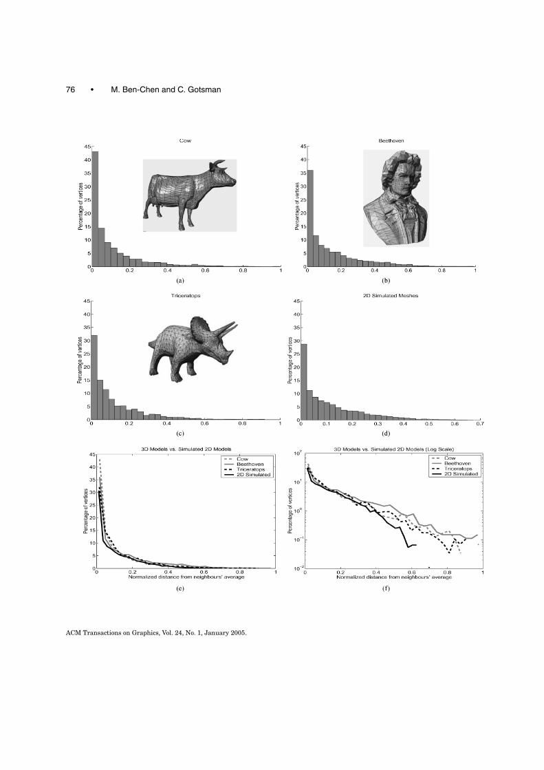
based on the fact that, in practice, a vertex will be close to the average of its neighbours. For example,a mesh geometry in which each vertex is located exactly at the average of its neighbours, containsno information beyond the locations of the boundary vertices. Indeed, this is also the nature of themean of our 2D distribution. Hence, the distribution of the quantity “the normalized distance betweena vertex and the average of its neighbours” across a mesh is a key measure of the efficiency of spectralcompression on this mesh. We have computed and compared the distribution of this quantity for anumber of well-known 3D meshes, and also for 2D meshes sampled from our distribution. Figure 9shows that these distributions are all very similar. While this does not prove anything about the moresubtle properties of the distributions, these results lend some support to our hope that our distributionalso reflects well the important properties of the 3D mesh distribution.

It is worth mentioning that defining multivariate normal distributions by specifying the coefficients ofthe conditional means is a well-known model [Besag and Kooperberg 1995], usually referred to as condi-tional autoregressive, or auto-normal formulation. Such models frequently arise in Bayesian networks,where they describe interactions between random variables that have neighborhood relationships.

6. CONCLUSION, DISCUSSION, AND FUTURE WORK

We have shown that under a few natural assumptions on the distributions of geometries, given 1Dand 2D connectivities, the covariance matrix of the mesh geometries is the inverse of the symmetricLaplacian matrix of that connectivity, and hence has the same eigenvectors (in reversed order). Thisimplies that spectral decomposition of meshes, which uses the eigenvectors of the symmetric Laplacianas the basis, is optimal.ACM Transactions on Graphics, Vol. 24, No. 1, January 2005.


Fig. 7. The difference matrix |L−1 − αC|/|αC|, color-coded. The darker the color, the closer to zero the value in the differencematrix. The maximal (white) entry is approximately 3.4.

Fig. 8. The “energy” contained in the first k coefficients, for a mesh with n = 1000 vertices. The graph shows∑

i=1…k c2i /

∑i=1..n c2

i ,where ci are the coefficients of the decomposition by the PCA basis (computed using the empirical covariance matrix), and thespectral basis. Note that this figure shows the coefficients’ energy for a single mesh, whereas our theory relates to the similarityof the coefficients on the average over many possible valid meshes.

On the practical side, to achieve an optimal decomposition, the geometries should be centered tohave a zero mean, before the decomposition. This is crucial since, as described in Section 3, PCA isoptimal only for a random vector X , which has a zero mean. The geometries as we described them donot have such a property, therefore they should be centered before decomposition by subtracting awaytheir mean, which can be shown to be Exp(X ) = L−1 BX —the “Tutte configuration” with the givenboundary, namely, where each interior vertex is at the centroid of its neighbors..





There are a few more directions that are worth exploring. These are described in the next sections.

6.1 Other Distributions

Our proof is based heavily on our assumptions about the distribution of meshes in one and two dimen-sions. The distributions that we impose are obviously not the only ones possible. In one dimension,one may use the same scheme as in two dimensions, and generate the geometries using a randombarycentric coordinates matrix. Another possibility is to define X i to be

∑ij=1 Y j /

∑nj=1 Y j , where Yi

are uniformly distributed random variables. This is guaranteed to generate a monotonically increasingsequence. The optimality proof in the one-dimensional case hinges on the key fact that the randomvariables X i − X i−1 are interchangeable, hence the proof holds for any distribution that satisfies thatcondition. Specifically, this is the case for both of the models just described, even though these donot generate uniform distributions on the class of valid geometries. It is encouraging to see that theoptimality result is not too sensitive to the geometry distribution.

In two dimensions, there are two main variations on our model. One possibility is not to use barycen-tric coordinates at all: For example, one can generate random X and Y coordinates, and keep only the(X , Y ) vector pairs that form a valid geometry. A geometry will be valid if all the triangles have thesame orientation. Obviously, this is not an efficient method to sample this distribution, since for largen, the probability that a random (X , Y ) pair will form a valid geometry is very small. The advantage ofthis process, however, is that it will generate geometries distributed uniformly over the class of validgeometries, but it is not clear whether our proof extends to this distribution.

Another possibility is to generate random 2D geometries by modifying the distribution of the barycen-tric coordinates matrix. For example, instead of being uniform spacings, the barycentric coordinates canbe wij = Yi/�i=1 . . d Yi, where Yi are independent, identically distributed, uniform random variables.However, here too it is not clear whether the optimality result will still hold.

Although our 2D optimality result was derived using properties of the normal distribution, which isjust an approximation of the true geometry distribution, we believe that the result actually holds forthe true distribution of the geometries, as in the 1D case, without resorting to normal approximations.This, unfortunately, will probably require a completely different proof.

For both 1D and 2D meshes, our proof is based on the fact that the inverse covariance matrix hasthe same eigenvectors as the Laplacian, and there is no constraint on the eigenvalues as long as thereverse ordering is preserved. This fact implies another way to apply our proof to other distributions:one can prove that the inverse covariance equals to some integer power of the Laplacian, or any otherfunction of the Laplacian that doesn’t change the eigenvectors and the order of the eigenvalues of theresulting matrix.

6.2 The Decay Rate of the Spectral Coefficients

For compression applications, it is important to know how fast the spectral coefficients decay to zero.This property relates directly to the rate/distortion relation of the compression, and is also known as“Energy Packing Efficiency”. Based on our proof that the Laplacian equals the inverse covariance up to aconstant, we can show that the spectral coefficients for the meshes treated here decrease on the average.This, in itself, is an important fact, since a priori there is no reason they should even decrease. Let X

←−

Fig. 9. The empirical distribution of the relative distance of a vertex from the average of its neighbours: (xi−Avg (x j ))2

Avg ((xi−x j )2)| j ∈ Neigh(i),

where xi is the value of the X coordinate of the i-th vertex. The graphs show the histogram of this value, for (a) the “Cow” model,(b) the “Beethoven” model, (c) the “Triceratops” model, and (d) 2D geometries sampled from the distribution described in thisarticle. All four distributions (a-d) are on the same plot, using linear (e) and log (f) scale.



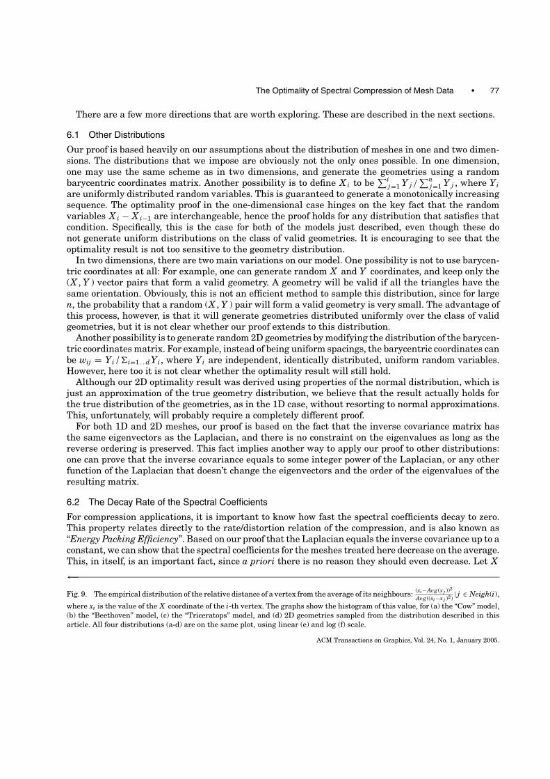
Fig. 10. 3D geometries with common connectivity and boundaries. (a) The barycentric coordinates matrix is (I − L′), where L′is the Laplacian L normalized to unit row sums, and the displacement has constant variance for all vertices. (b) The barycentriccoordinates matrix is (I − L′), and the displacement is smooth. It was generated by randomizing displacement values on theboundaries, and computing the displacement at each vertex by N = L−1 BN . (c, d) The displacement is computed as in (b),but random barycentric coordinates matrices are used (e, f) Random barycentric coordinates matrix and random Gaussiandisplacement with variance 1/n2, where n is the number of vertices in the mesh.

be a random geometry (column) vector, and C = �T X the corresponding spectral coefficient vector.By definition, � is the orthogonal matrix of the column eigenvectors of L—the mesh Laplacian—inincreasing order of the eigenvalues: L� = ��, where � = diag(µ1, . . , µn) is the diagonal matrixof L’s eigenvalues, in that order. We have proven that the geometry covariance matrix is Cov(X ) =αL−1. Hence Cov(C) = Cov(�T X ) = �T Cov(X )� = α�T L−1�. Now, since L−1 = ��−1�T , we obtainCov(C) = α�T ��−1�T � = α�−1. This means that the spectral coefficients are pairwise uncorrelatedand decrease on the average. Since, by definition, Exp(X ) = 0, this implies that also Exp(C) = 0, so thevariance of C is (α/µ1, . . , α/µn), which obviously decreases.

For the 1D, case, the exact eigenvalues of L are known, so we can find the decay rate of thesecoefficients. In 1D, the Laplacian is a symmetric tridiagonal Toeplitz matrix, whose eigenvalues areknown [Hartfiel and Mayer 1998] to be µi = 4 sin2( πi

2(n+1) ). For large n, the argument of the sin function



is very small, so the sin function may be approximated by its argument. This means that the inverseeigenvalues, and hence the spectral coefficients, decay like θ (1/i2).

6.3 Extension to 3D Meshes

In three dimensions, matters are more complicated. Just applying the barycentric method (15) to a(nonplanar) 3D boundary results in a smooth, featureless surface interpolating the boundary vertices.This is obviously not rich enough to capture interesting 3D shapes.

A possible natural extension of the 2D model, which allows for 3D features to emerge, is the followinglinear system: X = WX + N , where N is a random displacement vector, independent of X , andthe system has fixed boundary vertices. This means that each vertex is a convex combination of itsneighbors up to a displacement. The displacement can be any reasonable random variable, as long asit is independent of X . The variance of the displacement values will influence the smoothness of themesh. A smooth mesh can be created by randomizing displacement values on the boundaries, and thencomputing the displacement values on the internal vertices by computing N = L−1 BN , where L is theLaplacian, and BN are the displacement values on the boundaries. The barycentric coordinates matrixW can be generated by uniform spacings, as in the two-dimensional case. See Figure 10 for examples of3D meshes with different displacements and different barycentric coordinates matrices based on thismodel.

The optimality proof for the 2D case is based on the following two key properties of the multivariaterandom variable X : the normal distribution of the conditionals, and the linear conditional expectation.Both those properties carry over to 3D, when using the model we have proposed, due to the displacementsN being independent of X .

Obviously, such a 3D model is not really satisfying, since it cannot generate “real-life” meshes—nocows will be born from random barycentric coordinates and displacements. An interesting experimentmay be to generate a family of geometries from a connectivity, for example by using the “ConnectivityShapes” method [Isenburg et al. 2001]. Analyzing the distribution of geometries generated this waymay provide an insight for finding the optimal basis for “real-life” 3D meshes. Unfortunately, such ananalysis may be mathematically complex.

REFERENCES

ALEXA, M. AND MULLER, W. 2000. Representing animations by principal components. Comput. Graph. For. 19, 3 (Aug.), 411–418.ALPERT, C. J. AND YAO, S. Z. 1995. Spectral partitioning: The more eigenvectors, the better. 32th ACM/IEEE Design Automation

Conference, San Francisco, CA. (June) 195–200.ARNOLD, B. C., CASTILLO, E., AND SARABIA, J. 1999. Conditional Specification of Statistical Models. Springer-Verlag.BESAG, J. AND KOOPERBERG, C. 1995. On conditional and intrinsic autoregressions. Biometrika, 82, 4, 733–746.BERA, A. K. AND JARQUE, C. M. 1981. An efficient large-sample test for normality of observations and regression residuals.

Working Paper in Economics and Econometrics 40, Australian National University.CHUNG, F. R. K. 1997. Spectral graph theory. Conference Board of Mathematical Science 92. American Mathematical Society.CHUNG, F. R. K. AND YAU, S. T. 2000. Discrete Green’s functions. J. Combinator. Theo. A 91 191–214.DAVID, H. A. 1981. Order Statistics. 2nd Ed. Wiley, New York.FLOATER, M. S. 1997. Parameterization and smooth approximation of surface triangulations. Comput. Aided Geometr. Design,

14, 231–250.GOTSMAN, C., GU, X., AND SHEFFER, A. 2003. Fundamentals of spherical parameterization for 3D meshes. In Proceedings of ACM

SIGGRAPH 2003.GOTSMAN, C. 2003. On graph partitioning, spectral analysis, and digital mesh processing. In Proceedings of Solid Modeling

International.HALL, K. M. 1970. An r-dimensional quadratic placement algorithm. Manage. Science 17, 219–229.HARTFIEL, D. J. AND MEYER, C. D. 1998. On the structure of stochastic matrices with a subdominant eigenvalue near 1. Linear

Algebra and Its Appl. 272, 193–203.



ISENBURG, M., GUMHOLD, S., AND GOTSMAN, C. 2001. Connectivity shapes. In Proceedings of Visualization 2001.JOLLIFFE, I. T. 1986. Principal Component Analysis. Springer-Verlag, New-York.LAURITZEN, S. 1996. Graphical Models. Oxford University Press.KARNI, Z. AND GOTSMAN, C. 2000. Spectral compression of mesh geometry. In Proceedings of ACM SIGGRAPH 2000, 279–286.KOREN, Y. 2003. On spectral graph drawing. In Proceedings of International Computing and Combinatorics Conference

(COCOON’03). Lecture Notes in Computer Science, Vol. 2697, Springer Verlag.PRESS, W. H., TEUKOLSKY, S. A., VETTERLING, W. T., AND FLANNERY, B. P. 1987. Numerical Recipes. Cambridge University Press.PYKE, R. 1965. Spacings. J. Royal Statist. Soc. B, 395–439.RAO, K. R. AND YIP, P. 1990. Discrete Cosine Transform. Academic Press.RICE, J. A. 1988. Mathematical Statistics and Data Analysis. Brooks Cole Publishing.ROSSIGNAC, J. 1999. EdgeBreaker: Connectivity compression for triangle meshes. IEEE Trans. Visual. Comput. Graph., 47–61.TAUBIN, G. 1995. A signal processing approach to fair surface design. Proceedings of ACM SIGGRAPH ’1995, 351–358.TAUBIN, G. AND ROSSIGNAC, J. 1998. Geometric compression through topological surgery. ACM Trans. Graph. 17, 2, 84–115.TOUMA, C. AND GOTSMAN, C. 1998. Triangle mesh compression. In Proceedings of Graphics Interface, 26–34.TUTTE, W. T. 1963. How to draw a graph. In Proceedings of the London Mathematical Society 13, 3, 743–768.

Received July 2003; revised February 2004, June 2004; accepted September 2004


Documents

On the Optimality of Spectral Compression of Mesh Data