ON THE RELATIVE EFFICIENCY OF ESTIMATORS WHICHINCLUDE THE INITIAL OBSERVATIONS IN THE

ESTIMATION OF SEEMINGLY UNRELATEDREGRESSIONS WITH FIRST ORDER~AUTOREGRESSIVE DISTURBANCES

H.E. Doran and W.E. Griffiths

No. 13 - June 1981.

A substantial part of this work was done while Doranwas a Fellow of the Alexander yon Humboldt Foundationat the University of Bonn.

ISSN 0157 - 0188ISBN 0 85834 388 6

ABSTRACT

The generalized least squares estimator for a seemingly unrelated

regressions mode! with first order vector autoregressive disturbances

is outlined, and its efficiency is compared with that of an approximate

generalized least squares estimator which ignores the first observation.

A scalar index for the loss of efficiency is developed and applied to

a special case where the matrix of autoregressive parameters is diagonal

and the regressors are smooth. Also, for a more general mode!, a

Monte Carlo study is used to investigate the relative efficiencies of

the various estimators. The results suggest that Maeshiro 1980) has

overstated the case for the exact generalized least squares estimator,

because, in many circumstances, it is only marginally better than the

approximate generalized least squares estimator.

i. Introduction

Since the work of Prais and Winsten (1954) a great deal of attention

IKadiyala (1968), Poirier (1978), Beach and Mackinnon (1978), Spitzer (1979),

Chipman (1979), Maeshiro (1979), Park and Mitchell (1980), Doran (1981)I has

been paid to the relative efficiency advantages of retaining the initial obser-

vation when estimating a regression model with a first order autoregressive

disturbance. Despite this work on the single equation model, the same problem

in seemingly unrelated regressions with first order autoregressive disturbances

IParks (1967), Guilkey and Schmidt (1973)I does not appear to have attracted

much interest. Two exceptions are the papers by Beach and Maekinnon (1979)

and Maeshiro (1980). Beach and Mackinnon, under the assumption of normally

distributed disturbances, advocate maximum likelihood estimation which retains

the initial observations and which, through the Jacobian term, constrains the

parameter estimates to lie within the stationary region. However, as they

~oint out, except in a very~special case, it is impossible to concentrate any

parameters out of the likelihood function and numerical maximization of the

function with respect to all th~ parameters is likely to be computationally

difficult. An alternative procedure which retains the initial observations,

but which does not ensure the estimates satisfy the stationary constraint, is

to use a properly constructed generalized least squares (GLS) estimator.

Computationally, this estimator involves more steps than the approximate GLS

estimators suggested by Parks (1967) and Guilkey and Schmidt (1973), but it is

likely to be less of a problem than the maximum likelihood estimator. If the

single equation results and the evidence provided by Maeshiro (1980) are any

guide, it could lead to some substantial gains in efficiency. Using a two

equation model with one explanatory variable in each equation, the nonstationary

disturbance assumptions employed by Parks (1967), and a knourn autoregressive

process, Maeshiro (1980) finds that the approximate GLS estimator which ignores

the initial observations can be considerably worse than ordinary least squares,

particularly when the explanatory variables are trended.

The purpose of this paper is similar to that of Maeshiro’s, namely, to

investigate the relative efficiency of "GLS estimators" which use, and do not

use, the initial observations. However, our approach is different. We assume

that the disturbances are stationaryI and that the autoregressive process is

not necessarily diagona!; we use a larger model (three equations with two

explanatory variables in each equation); and, using Monte Carlo experiments,

we concentrate on the situation occurring in practice where the autocorrelation

and variance parameters must be estimated. Also, under the assumption that

the autocorrelation and variance parameters are known, we follow Doran (1981)

and develop a scalar index for the loss of efficiency resulting from omission

of the initial observations. This index can be used for a model with any

number of equations and any number of explanatory variables in each equation.

For the special case of a two equation model with a diagonal autorezressive

process, we examine the index in detail, and this provides some valuable insights

into the various factors which influence the loss of efficiency.

In Section 2 the model and appropriate estimators are discussed. In

Sections the scalar index of loss of efficiency is derived and used to investigate

loss of efficiency, for the case where there are two equations and the autoregressive

process is diagonal. Results of the Monte Carlo experiments using the more

general model are reported in Section 4, followed by some concluding remarks

in Section 5.

- 3 -

2. The Model and Estimators

Following Guilkey and Schmidt (1973) we consider N seemingly unrelated

regression equations of the form

Yi = XiBi + ui’ i = 1,2,...,N. (2.i)¯

where Yi is a (T x I) vector of observations on the i-th dependent variable,

X. is a (T x K.) nonstochastic matrix of observations on K. explanatoryi i i

variables, 8. is a (K. x I) vector of coefficients to be estimated and u. isI i

a (T x i) vector of random disturbances. The system can be written more

compactly as

y= XB +u (2.2)

y~) X is block diagonal of dimensionwhere y’ : (Yi’ Y2’ "’’’ ’

(NT x K), where K :N

[ Ki, B’ :i:l

(6i, B~, ..., B~) and u’ : i , ’)(U , U2, ..., uN ¯

Let u(t) be an (N x i) vector containing a disturbance from each equation

for the t-th time period and suppose

u(t) : Ru(t-l) + s(t)’ t-: 0,+i, +2, ...,(2.3)

where R is an (N x N) matrix with (i,j)th element given by p.. and±] ~(t)

an (N x i) vector of random disturbances such that E[s(t)] = 0 and

is

IE ift : s

E[g(t)~(s~][0 if t ~ s.

(2.4)

We assume the process in equation (2.3) is stationary. This is true if the

roots of Izl RI = 0 are less than one in absolute value. Also, it implies

that the covariance matrix for u(t) does not depend on t. Let this covariance

matrix be given by E[u(t) u~t)] : 0, and let the covariance matrix for the

complete (NT x i) disturbance vector be given by E[uu’] = ~.

- 4 -

If R and Z are known the GLS estimator for 6 can be calculated by first

finding a matrix P such that B2P’ = Z @IT and then applying the seemingly

unrelated regressions estimator [Zellner (1962)] to the transformed model

y* = X*6 + u*, (2.5)

where y* = Py, X* = PX and u* = Pu. This GLS estimator is

~ : (X,p,(E-I@IT)PX)-Ix’p’(E-I@IT)py, (2,6)

and its covarianee matrix is

V(~) : (X’P’(Z-I~IT)PX)-I (2.7)

A suitable matrix P is given by

PII PI2 "’" PIN

P21 P22 "’" P2N

PNI PN2 "’" PNN

where

( TxT )

a.. 0 0 ... 0 0-11

Pii i 0 ... 0 0

o -Pii i ... o o

0 0 -Pii i

(TxT)

Pij

-Pij

0 O-

0 0

0 0

,

and the elements of

(NxN)

(2.8)

2are chosen such that Z = AO A’.

Later we shall return to how the elements of O and A can be derived given

R and Z. First we shall note the form of the transformed variables in

equation (2.5). Transformed observations on the dependent variable, for

example, are given by

i

Y~I : j~l~ijYjl’i : i, 2, ..., N (2.9)

and

N

~i : i, 2, ..., N,

(2.10)PiJYjt-l’ t = 2, 3, ..., T.Y~t : Yit j:l

- 6 -

An important difference between the transformations in (2.9) and (2.10) is

that the transformed initial observations in equation (2.9) will, as we shall

see, depend on both the Pij and the elements of ~, while in equation (2.10) the

transformed observations depend only on the Pij"

Because of this, rather than use the GLS estimator given in equation (2.6),

it is easier to just use the observations in equation (2.10) to obtain an

approximate GLS estimator. Let Pijo be the ((T - i) x T) matrix obtained by

deleting the first row in Pij and let Po be the (N(T i) x NT) matrix containing

Pijo in the (i, j)th block. The approximate GLS estimator is given by

~o : (X’Pg(Z-i~IT-i)PoX)-ix’pg(?’-i~IT_i)PoY (2.11)

and its covariance matrix is

V(~o) = (X’Pg(Z-i~IT_i)PoX)-i (2.12)

We are interested in evaluating, for a number of alternative X, R and ~,

v(~) V(~o). In addition, and more importantly, wehow much "less" is than

wish to determine whether or not the efficiency difference persists°when, in

and 8o, the pfj and the oij (the elements in Z) are replaced by estimates.

Before turning to these questions we shall indicate how the ~ij can be

obtained from the Pit and oi~’ and define estimators b and bo which use^ ^estimates of the pi~] and o~,lj and which are the counterparts of 8 and 8°

respectively.

Following Guilkey and Schmidt (1973) we can use the fact that 0 = ROR’ + Z

to solve for the elements of 8 from

vec(@): (I - R@R)-ivec(Z), (2.13)

where vec(.) is a vector obtained by stacking the columns of a matrix. Then,

to obtain A we find lower triangular matrices H and B such that E = HH’ and

~ = BB’ [Graybill (1969, p.299)] and from these, A = HB-I.3

- 7 -

To obtain the estimator b we can use one of the methods described by

Guilkey and Schmidt (1973), modified to include the initial observations.

The steps are:

(i) Apply least squares to each equation and obtain the least squares

residuals

ui = (IT - Xi(XIXi)-IxI)Yi ’ i = i, 2, ..., N.

(±i)^ ^ A

For each equation regress uit on (Ult_l, u2t_l, ..., UNt_l).

^ ^ ^

This yields estimates Pil’ Pi2’ "’’’ PiN’

notation, ~.

i = i, 2, ..., N, or, in matrix

(iii) Let ~o be the matrix Po with the Pij replaced by the estimates

obtained in step (ii) and regress ~oy on ~oX to obtain the (N(T - i) x i)

residual vector (s12’ s13’ "’’’ SiT’ ~22’ "’’’ S2T’ "’’’ gN2’ "’’’ ~NT)"

(iv)^

Estimate E by Z with elements

^ T ^ ^

oij = [ sitsjt/(T - 1) .t=2(2.14)

(v) Use the elements of ~. and R to find estimates 0 and A of 0 and A^ ^

respectively and use P and A to form P, the complete transformation matrix.o

(vi) Apply the seemingly unrelated regression estimator to the^

observations Py and PX. This yields the estimated generalized least squares

(EGLS) estimator

b : (X’~’ (~-I@IT)~X)-Ix’~’ (~,-l~IT>~y .

The approximate EGLS estimator suggested by Guilkey and Schmidt Can be

obtained by omitting steps (v) and (vi) and using instead

bo : (X’~(~-I@IT_I)~oX)-Ix’~(~-I~IT_I)~oy¯ (2.16)

- 8 -

3. An Index of Loss of Efficiency

In this Section we develop an index for the loss of efficiency which^occurs when the approximate GLS estimator 8° is used instead of the GLS estimator

^

B. Following Doran (1981) we define a~scalar index of loss of efficiency by

VoI-Ivl(3.1

where V = V(~ ) and V = V(B) are given by (2.12) and (2.7) respectively.o o

It is shown in Appendix A that

a : (-l)Nf(-l) - 1 , 3.2

where f(~) is the characteristic function of an N x N matrix P. That is,

3.3

where

p = (QA)(X’VoX)(QA)’ , 3.4

Q,Q : E-I , 3.5

and

i, ,)x’ = diag(x , x2, ..., xN ,

with x~ being the K.-row vector of the first observaiton on the regressori

variables of the i-th equation. The matrix A has already been defined in

(2.8),

If we expand the characteristic function f(B) in the form

NN N-i

f(~) : ~ + I (’llih’~ ’ (3.6ii=l

then from (3.2) we have that

N~ = ~ hi

i=1(3.7)

- 9 -

The coefficients h. may be obtained using the rules for the differentiation ofI

determinants [see, for example, Dhrymes (1978, p.470-471 and p.533-534)].

It is readily shown that

hI = tr(~), h2 = { [tr(~)]2 -tr(~2)}/2, hN = det(~)

Thus, when4

N = i, ~ -- tr(~) = det(~) _= ~

: _i (1 - ~2)x’2

: (i - )x’(X’x)-lx

N : 2, ~ = tr(~) + det(~)

N : 3, e : tr(~) + ~[tr(~)]2 - tr(~2) }+ det(~) .

From the definition (3.4) of ~ it is clear that the sample size T only enters

through the variance-covariance matrix V . Hence, under the usual assumptionO

that lim T-Ix’~-Ix is a finite nonsingular matrix, ~ is of order T-I.

Considering the expression for ~ when N = 3, it is clear that

hI : O(T-I), h2 : 0(T-2) and h3 : 0(T-3).

It seems reasonable to infer that for general N, h. = 0(T-i).i

fairly small T, the dominant term in ~ will be hI = tr(~). We wil! thus

adopt as our measure of inefficiency e, defined from now on by

Thus, even for

~ : tr(~) (3.8)

3.1 Loss of efficiency when R is diagonal and the regressors are smooth

In this subsection we consider the special case where R is diagonal and

the regressors are "smooth". The assumption of a diagonal R has been popular

in the literature [Parks (1967), Kmenta and Gilbert (1970), Maeshiro (1980)]

- i0 -

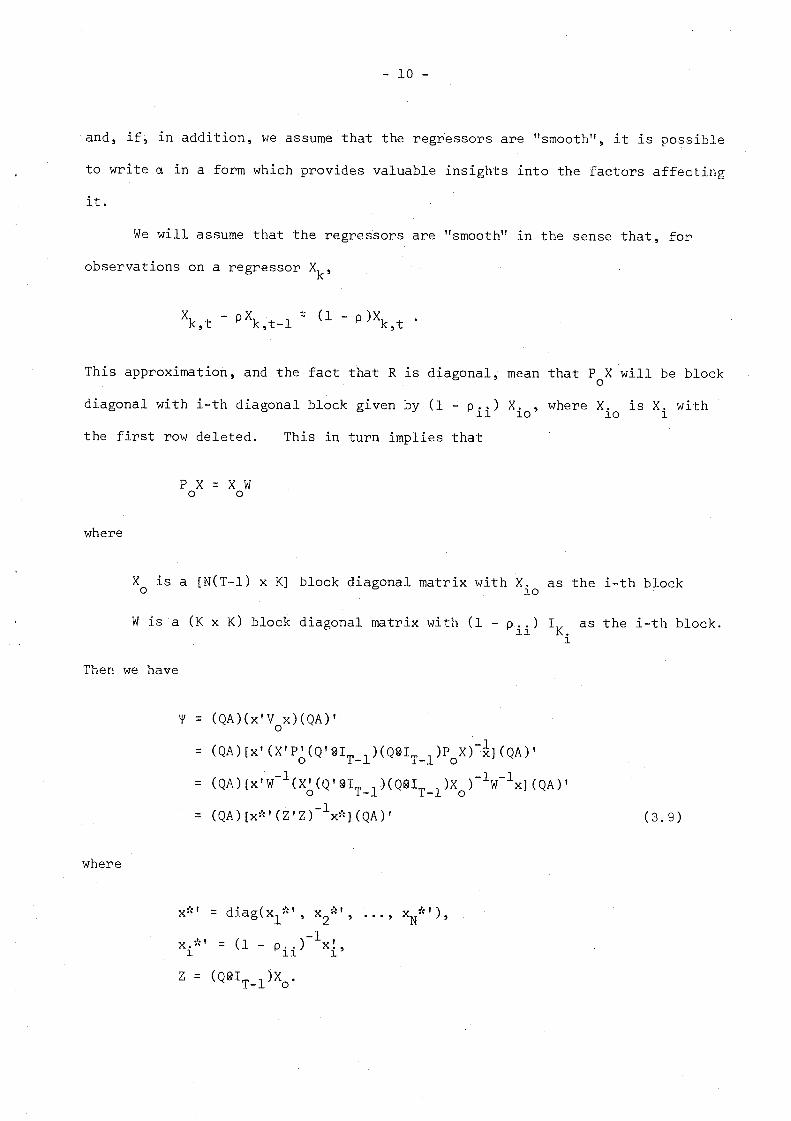
and, if, in addition, we assume that the regressors are "smooth", it is possible

to write e in a form which provides valuable insights into the factors affecting

it.

We will assume that the regressors are "smooth" in the sense that, for

observations on a regressor Xk,

Xk,t - PXk,t_I -" (i - P)Xk,t

This approximation, and the fact that R is diagonal, mean that P X will be blocko

diagonal with i-th diagonal block given by (i - Pii) Xio, where X.~o is X.~ with

the first row deleted. This in turn implies that

P X= XWo o

where

X is a [N(T-I) x K] block diagonal matrix with X. as the i-th blocko io

W is a (K x K) block diagonal matrix with (i - Pii) IK. as the i-th block.i

Then we have

~ : (QA)(X’VoX)(QA)’

: (QA)[x’(X’P~(Q’~IT_I)(Q~IT_I)PoX)’~](QA)’

= (QA)[x’W-I(x~(Q’@IT_I)(Q~IT_I)Xo)-Iw-Ix](QA),

= (QA)[x*,(Z,Z)-Ix*](QA), (3.9)

where

¯Xl,, x2~" XN*’x*’ = dzag( , ~’ )

xi*’ : (i - p [.,

Z : (Q~IT_I)Xo.

- Ii -

For example, if N = 2, and we use the fact5 that if the regressors are

appropriately scaled and R is diagonal, Z may be interpreted as a correlation

matrix, we have

andr. =

2

6An appropriate matrix Q, defined by (3.5), is

(3.10)

-~ )-½where II = (i + r) ~ and 12 = (i - r are the eigenvalues of Z

Z~Z =

2(I1

+ 1~~)×ioXio (Ii -2 , 2 2 ,

- 12 )X20XI0 (I1 + 12 )X20X20~

-i Then,

(3.11)

We may now proceed in an analogous way to Doran (1981). Suppose

61, 62, ..., 6K are t~e eigenvalues of Z’Z. Then there exists an orthogonal

matrix C such that

Z’Z = CDC’,

where D : diag(61, 62, ..., 6K) ;

If we define the scaled eigenvalues

K6i* = 6i/j!16j ’

then

6i* = 6i/tr(Z’Z) , and

where

(Z,Z)-I : CD*-Ic,/tr(Z,Z) ,

[~ : diag(61 , 62 , ..., 6K ).

- 12 -

Now by (3oli)

~ 222)[

,tr(Z’Z) = (II + I tr(Xl0Xl0) + tr(X~0X20)]

_ (T-l) [1~112 + 1~212~(1-r2)

(3.13)

where

T

I ~il 2 = (T-1)-i Zj:2 Ix’jit 2 (i : 1,2)

and

x~. is the j-th observation on the regressors in equation i.

We are now in a position to decompose (3.9) into components similar to

those obtained by Doran (1981). Substituting (3.12) and (3.13) into (3.9),

after some elementary algebra we obtain

~ :K(I - r2)

(QA)L(QA)’ (3.14)

(t-1)[I~.112 + I;,212]

where

£.. : (L).. : ] m.. (i, j : i, 2) , (3.15)1] l] (l-Pii) (l-pj j )

and the elements m.. are of the form

K

mi] : K-I £!i ~]

where 0 S lwij£1 S !. The numbers wij£ depend only on the orientation of

the vectors x! to the principal directions of Z’Z. Thus, the m.. do noti ~]

depend on Pll or P22"

- 13 -

Equations (3.14) and (3.15) illustrate how the loss in efficiency depends

on

m/(T-1),

(ii)

the number of regressors relative to the number of observations,

the length of the vectors containing the initial observations

relative to the average squared length of the vectors containing the ~emaining

observations,

I×j_l I x:l /

(iii) the "multicollinearity factor", m...

The influence of P lI’ P22 and r, and the precise dependence under (ii), will

also depend on the matrix QA. In Appendix B an explicit expression is derived

for tr[(QA)L(QA)’], and we obtain finally that ~ : tr(~) is given by

K(1-r2)

I %!

2 2 tlmo 2 ) 2~. ~ ii (1-p jj)

i=! j=l (l-Pii)(l-P(3.16)

where fij = fij(Pll’ P22’ r), (see Appendix C) and

fll’ f22 ÷ i1

f12 ÷ 0

as P ll or P22 ÷ i .

It is clear that ~ will become large when either Pll or P22 is close

to unity. As ~ is symmetric with respect to Pll and P22’ to gain a feel for

(3.16) we need only consider the case Pll ÷ i, when (approximately)

K(1-r2) l-p ii )mll

(i-Pii)2

Recalling that ~ is expressed in scaled variables, we obtain (reverting to the

- 14 -

original variables) that as Pll ÷ i,

2 !K(i-r2) (i-p ii) I xiI 2/oii

)2(T-i) (i-p ii [l~il i+I~2

mll

2/o~21

(3.17)

This expression for e gives rise to the following remarks on loss of efficiency

when approximate GLS is used instead of GLS:

(i) The correlation r between the disturbances enters mu!tiplicatively

2through the factor l-r . Thus, if Irl is reasonably close to i,

(ii)

loss of efficiency will not be as severe.

very sensitive to the value of r.

The effects of large differences in I~ll

Otherwise, ~ is not

and 1~21 are

easily identified. If 1~212/o22 << I~iI2/oll, then apart from

the factor (l-r2), loss of efficiency is dominated by the first

equation alone. This case is discussed in Doran (1981). In

particular, ~ will be almost independent of the value of P22" On

the other hand, if I~iI << I~2 2/o22, ~ will tend to be

proportional to (I~ll )/(I~21 2) and will therefore be less.

The relatively large loss in efficiency incurred by Pll being close

to unity is offset by this factor.

The above remarks give some additional insights on Maeshiro’s (1980,

Table i) results. Firstly, he only tabulates results for the case r = 0.65, but

not those for r = 0.0 or r = 0.975. Because of the miltiplicative factor (l-r2)

we suspect that his results would show ARTZEL (that is, approximate GLS in our

terminology) to be even less efficient when r = 0.0 (but not too much), but

almost as efficient as SURGLS (our GLS) when r = 0.975. Secondly, an examination

of the results for the trended case show asymmetry as Pll ÷ i and P22 ÷ i.

2/o22’

£or Maeshiro’s data, 1~2J is less than .0051~11 , and according to <3.16)

we would expect ARTZEL to be more efficient as P22 ÷ i. This effect is very

obvious in his results. Thirdly, again because of the relative magnitudes of

- 15 -

I~ll 2/all and I R21 ~2’ we would expect the efficiency of ARTZEL relative to

SURGLS to be almost independent of P22 when Pll is large. From the last column

of Table 1 it can be seen that as P22 varies from 0.i to 0.9, the efficiency

of ARTZEL only varies from 0.41 to 0.44.

Finally, we must take exception to Maeshiro’s statement that "the

retention of the first observations in the estimation of a SUR model is as

critical as in the case of a single’equation model". We believe that this

statement is far too sweeping as the relative efficiency of approximate GLS

will depend on the relationship of I~iI2/all, I~21 2/~22 and r.

4. Monte Carlo Experiments

The analysis of the previous section gives some useful insights about

when approximate GLS is likely to be inefficient, but is limited in three respects.

(i) The parameter matrices R and Z have been assumed known.

(ii) R has been assumed to be diagonal.

(iii) The regressors have been assumed to be smooth.

Monte Carlo experiments were conducted to examine the relative efficiency

of a number of competing estimators in less restrictive conditions. Of special

interest were the questions of efficiency when R and Z were not known, and the

effects of a misspecification of R.

The model consisted of three equations (N = 3) and two explanatory variables

plus a constant in each equation, so that 8 was of dimension (9 x i). The

explanatory variables were fixed in repeated samples and two settings were used:

XI: X’s independent and uniformly distributed

Xt = Zt x scale factor

X2: X’s trended and With correlations between 0.7 and 0.9.

Xt = [(l.05)t(l + (Zt-O.5)/z)] x scale factor.

In the above Zt is a uniform random variable on the interval zero to one, z was

set to give a fair degree of multicollinearity, and the scale factor was set to

16 -

make the "true R2’s’’ about 0.85. Based on t~e results of Doran (1981) and

Maeshiro (1980), one would expect the loss of efficiency from omitting the

first observation to be greater for the setting X2 where the variables are

trended and exhibit some multicollinearity, than for the setting XI. One

7sample size (T = 20) was used.

Three settings for the disturbance covariance matrix were employed,

namely

with r = 0.0, 0.2 and 0.8. A total of seven settings for R were used and,

classifying them into three categories, these were

(i) R diagonal with elements

(0.9, 0.6, 0.4), (0.5, 0.4, 0.3), (-0.9, 0.6, 0.4).

(ii) R non diagonal, of the form

2 2"(UI+P2+211Pl) ll+2Ulj

With this construction, R has eigenvalues

(~i’ ~l+iP2’ Ul-iP2)" The triplet (~I’ ~i’ P2) was given values

(0.9, 0.6, 0.6), (0.5, 0.6, 0.6) and (-0.9, 0.6, 0.6).

(iii) R = O. This is the case of zero autoregression.

The form of R under (ii) was a convenient way of setting up a nondiagonal R with

an eigenvalue close to the boundary of the stationary region (±0.9). It was

suspected that, with such a setting of R, the dropping of the first observation

would lead to a greater efficiency loss than for settings of R where the

eigenvalues were well within the stationary region.

- 17 -

For each combination of regressor variables, R and ~ (42 combinations),

one hundred samples were generated, and the means and mean square errors of

eight estimators were estimated. Those considered were

b

b

~(i) : (X’X)-Ix’y (OLS)

~(2) : (X’(~-I~I)X)-Ix’(~-I@z)y (SUR)

: ~(3) : (X’Pg(Z-I~IT_I)PoX)-Ix’pg(z-I%IT_I)Poy (approx. GLS)

: ~(4) : (X’P’(~.-I@IT)PX)-Ix’p’(F,-I@IT)Py (GLS)

= ~(5) = (X’~(~.-l@ZT_l)~oX)-ix’~(~-l@ZT_l)~oy (approx. EGLS)

: ~(6) : (X’~’(~-I@IT)~X)-Ix’~’(~-I@IT)~y (EGLS)

~(7) = ~(5) with R assumed to be diagonal^

~(8) = 8(6) with R assumed to be diagonal

To summarize the relative efficiency of each estimator we took the ratio of the

mean square error of each coefficient for each estimator to that of GLS and,

8for each estimator, these were averaged over all coefficients.

The results for r = 0.8 are presented in Table i. We chose not to report

the results for r = 0.0 and r = 0.2 since, in line with the analytical results

of the previous section, the effect of different values of r turned out to be

fairly weak. 9 In Table ~i, the rows and columns are numbered for ease of reference

with the row numbers corresponding to the eight estimators. For example, entry

(6, ii) refers to the case of the EGLS estimator applied to the model in which

R is non-diagonal with roots (-0.9, 0.6, 0.6) and the regressors are not trending.

The following conclusions emerge:

i, Some efficiency is lost by ignoring the first observations, but not

very much. The loss is greatest when a root of R is close to +i and the

regressors are trending. (Compare rows 3 and 4.)

2. The loss of efficiency in moving from the infeasible estimatdrs GLS and

approximate GLS, to the feasible estimators EGLS and approximate EGLS,

is very large. This is particularly so when R is non-diagonal, and

- 18 q

when a root of R lies near +i. (Compare rows 4, 6 and 8; and 3, 5 and

7.)

The inefficiency of approximate EGLS relative to EGLS is negligible.

When R and Z are estimated, it is better to assume R is diagonal, even

when it is not (compare rows 5 and 7, 6 and 8 for columns 7 to 12).

When R = 0~ assuming diagonal R results in only a slight loss in

efficiency (compare rows 2 and 7, and rows 2 and 8 for columns 13 and 14).

In no case can the use of OLS be justified.

5. Concluding Remarks

In this study we have examined the efficiency of approximate GLS procedures

(both feasible and infeasible) relative to the corresponding GLS procedures

for seemingly unrelated regression models with a vector autoregressive disturbance.

In the case of a single equation, application of GLS involves negligible extra

effort relative to approximate GLS. However, in the case of multiple equations

this is not the case. Our interest is inwhether the extra efficiency obtained

by using GLS is worth the considerable extra labour.

This question has also been considered by Maeshiro (1980). Arguing on

the basis of results obtained when the autoregressibe parameters are kno~, he

concludes that "the only viable and reliable mult~equation estimator of a SUR

model with AR(1) disturbances is SURGLS".

The findings of this study strongly disagree with this statement. With

the three equation model with two explanatory variables in each equation, we

did not find any cases where approximate (infeasible) GLS was considerably

inferior to (infeasible) GLSo This is despite the fact that we had setups

where the explanatory variables were trending and the roots of R were close

to ±I. The worst cases were when a root of R was close to +i (columns i, 2,

7and 8 of Table i); but even in these cases approximate GLS was always at

least 78 per cent efficient. When we moved from the infeasible tothe feasible

estimators we found that the resulting loss in efficiency completely swamps the

gain in efficiency Obtained from using (feasible) GLS rather than approximate

(feasible) GLS. Also, relative to (feasible) GLS, the approximate estimator

was in all cases at least 85 per cent efficient~ and in most cases 95 per cent

efficient.

Our experiments also indicated that the best strategy is always to assume

a diagonal autoregressive structure. When there is no autoregression there

is very little loss in efficiency. When there is non-diagonal autoregression~

this mis-specification seems to result in substantial gains in precision.

Appendix A

The loss of efficiency ~ is defined by

wh ere

V-i = X’P’(F.-I~IT)PX

V -i : X,pg(~-i~iT_i)P Xo o

Consider

M : P’(Z-I~IT)P - Pg([-I@IT_I)P°

and let M.. denote the (i, j) T x T block.i]

Now the (i, j) blocks of P and P are related through P]~±j : (p~j,± P’ ) whereo oij

Pij : (~ij’ O, ..., 0). Thus, terms like

oijPij = ( ,p, .p .)

’ Pij °ij PijPij + oil oil

will differ from oijP’..P .., only in the (i i) element.oil ol] ’

M.. must be zero everywhere except in the (i, i) element.i]

Defining the T-vector

This implies that

’ = [i, O, O, O]IT ..., ,

we have that

!

Mij : ~ij IT IT ’

where iij is some scalar.

Thus,

!M : i@ I,T iT (AI)

where

(!)ij : %ij"

21-

appropriately partitioning the matrices P ~.-I~ITBy P~ O

be easily shown that

and Z-I~IT_I, it can

¢ = A’z-IA (A2)

Pre-multiplying (AI) by X’ and postmultiplying by X,

X’MX = V-i -V-io = X’(~@ITI})x

where

x’ = diag(xl, x~ ..., x~) (A3)

and x! is the Ko row vector of the first observation on the regressors of thei i

i-th equation.

Thus

V-I = V-I + xlx’ (A4)o

Taking the determinant of (A4),

~ : I IK + VoX~X’{ (AS)

The KxK matrix V xlx’ is of rank N at most and N < K, which implies thato

V xlx’ is singular. In order to express (AS) in terms of non-singular matriceso

we use the following standard matrix algebra result [see for example Dhrymes

(1978, p.472)].

Suppose A is KxN and B is NxK with N < K.

Then

Thus, setting ~ = -i, A = V x, B = ix’ (A5) may be written in the formo

22 -

iv:if fIN * ~X’VoXI(A6)

The NxN matrix ix’V x is non singular.o

Q,Q = ~-1, then

If we define a matrix Q to satisfy

@ : (QA)’ (QA)

and (A6) may be written as

where

~ : (QA)(x’V x)(QA)’o (A7)

[see Dhrymes (1978, p.470)].

Thus, defining the characteristic function f(~) of ~ by

f(~) = IuIN - ~1,

it follows that

1 : (-l)Nf(-l) - i. (A8)

- 23-

APPENDIX B

In Section 2 the method for obtaining A is outlined. The steps are

(i) Solve O = R@R’ + Z for O;

(ii) Factorize Z = HH’ and ~ = BB’ where H and B are lower triangular;

(iii) A =~HB-I

When R is diagonal application of this procedure is particularly simple.

Using the scaled version of Z, given by

we obtain

Ill_p ii

2 ) -1

(1-p lip 2 2 )-i

r ( l-p lip

2)-i(l-p 22

il-r2 )½1

and

where

-iB

LF½" ,2.½

i IA ~i-Pll ) 0

A l-r(l-PllP22)-l("l-pl12"½) (l-Pl12)-

A -= deto :)2 r2(l_Pl12)(l_P222)(l’PllP22 -

2 2(1-Pll)(1-P22 )(1-Pl!P22)2

(BI)

24 -

Thus,

A = HB-I

Denoting by aij the elements of A (with a12 = 0), we obtain

2 2[(QA)L(QA)’]ii : b~21[(all+a~l) [ll+2a22(all+a21).[12+a22122]

(B2)

[(QA)L(QA)’]22 : ½12 22 [ ( all-a21 ) 2£11-2a22 ( all-a21 )£12+a22~22]

As2 = 2(i_r2)-i 2 2 _2r(l,r2)-i

21+I 2 .and A i-i 2 =

2 2 2tr[(QA)L(QA)’] : (l-r2)-l[(all+a21-2ralla21)~ll+a22~22+2a22(a21-rall)~12]

On substitution of a.. from (C2) we obtain

tr[ (QA)L(QA)’ ] :2 (l-p ii jj

( ) (]_-p )i:l j:l l-Pii jj

where fij -= fi~(Pll’ P22’ r)

and

fll(Pll’ P22’ r) = i +

r2(l-p211) (i-p222)

2 _ 2 2[ (1-P llP 22) r2(1-Pll) (1-P 22)]

(B3)

f22(Pll’ P22’ r) =

¯)2( l-p lip 2 2

)22 2

[(1-PllP22- ~2(1-Pl].)(1-P22)]

(B4)

25 -

f12(~ll’ ~22’ r) =

2)½( 2 ~-2r(l-Pl! I-P22) 2(I-PlIP22)

)22

~2)][ (I-PlIP22 r2(l-Pll) (I-P

(B5

As PlI’ P22 ÷ I, fll ÷ i, f22 ÷ i and f12 ÷ O.

- 26 -

References

Beach, C.M. and J.G. Mackinnon, 1978, "A Maximum Likelihood Procedure for

Regression with Autocorrelated Erroms!’, Econometrica, 46, 51-58.

Beach, C.M. and J.G. Maekinnon, 1979, "Maximum Likelihood Estimation of

Singular Equation Systems with Autoregressive Disturbances",

International Economic Review, 20, 459-464.

Chipman, J.S., 1979, "Efficiency of Least Squares Estimation of Linear Trend

when Residuals are Autocorrelated", Econometrica, 47, 115-128.

Dhrymes, P.J., 1978, Introductory Econometrics, New York: Springer-Verlag.

Doran, H.E., 1981, "Omission of an Observation from a Regression Analysis:

A Discussion on Efficiency Loss, with Applications", Journal of

Econometrics, forthcoming.

Graybill, F.A., 1969, Introduction to Matrices with Applications in Statistics,

Belmont, Calif: Wadsworth.

Guilkey, D.K. and P. Schmidt, 1973, "Estimation of Seemingly Unrelated

Regressions with Vector Autoregressive Errors", Journal of the American

Statistical Association, 68, 642-647.

Kadiyala, K.R., 1968, "A Transformation Used to Circumvent the Problem of

Autocorrelation", Econometrica, 36, 93-96.

Kmenta, J. and R.F. Gilbert, 1970, ’,Estimation of Seemingly Unrelated Regressions

with Autoregressive Disturbances", Journal of the American Statistical

Association, 65, 196-197.

Maeshiro, A., 1979, "On the Retention of the Firs~ Observation in Serial

Correlation Adjustment", International Economic Review, 20, 259-265.

Maeshiro, A., 1980, "New Evidence on the Small Sample Properties of Estimators

of SUR Models with Autocorrelated Disturbances: Things done half-way

may not be done right", Journal of Econometrics, 12, 177-188.

Park, R.E. and B.M. Mitchell, 1980, "Estimating the Autocorrelated Error Model

with Trended Data", Journal of Econometrics, 13, 185-202.

Parks, R.W., 1967, "Efficient Estimation of a System of Regression Equations

when Disturbances are Both Serially and Contemporaneously Correlated",

Journal of the American Statistical Association, 62, 500-509.

Poirier, D.J., 1978, "The Effect of the First Observation in Regression Models

with First-Order Autoregressive Disturbances", Applied Statistics, 27,

67-68.

- 27

Prais, S.J. and C.B. Winsten, 1954, "Trend Estimators and Serial Correlation’~

Chicago: Cowles Commission Discussion Paper No.383.

Spitzer, J.J., 1979, "Small-Sample Properties of Nonlinear Least Squares and

Maximum Likelihood Estimators in the Context of Autocorrelated Errors’’,

Journal of American Statistical Association, 74, 41-47.

Zellner, A., 1962, "An Efficient Method of Estimating Seemingly Unrelated

Regressions and Tests of Aggregation Bias", Journal of the American

Statistical Association, 57, 348-368.

Footnotes

iMaeshiro avoided the assumption of stationary disturbances because he thought

that, under this assumption, calculation of the covariance matrix of the GLS

estimator would require a large matrix inversion. However, as demonstrated in

Section 2, this is not the case.

/i 22When N = i, A, 0 and Z are scalars and it is easily seen that A = - p

3The diagonal elements of H and B are chosen to be positive, ensuring the

uniqueness of A.

4The expression for ~ when N = i is the same as that in Doran (1981).

51t is straightforward (though tedious) to show that if X. (i = i, 2, ..., N) isi

transformed to Xi/oii2, K and ~ are unchanged and ~ becomes a correlation matrix.

6Q is not unique. However, it is easily verified that, regardless of the

choice of Q satisfying (3.5), the characteristic function (3.3) is unique.

7In the preliminary stages of the development of the computer program we also

examined a model with two equations, and two explanatory variables plus a constant

in each equation. Two sample sizes (T = 20 and T = 40) were employed, and our

f~dings were consistent with those reported below.

8This measure of efficiency differs from that used to derive the analytical

results of Section 3, but it was more convenient from the standpoint of the

Monte Carlo experiment.

91nterested readers may obtain the full set of results from the authors.

0

II0 0 LO ~0 ~

0 ~

,--I CO 0 0 -.-I" ~ LO 00 O0 0 0 LO O~ CO C)

O0 0 b’- 0 ~ 0 -~,--’1 O0 0 0 ~ ~ ~