NASA Contractor Report 191546/ o2o G

On the Use of the Noncentral

Chi-Square Density Functionfor the Distribution of

Helicopter Spectral Estimates

Donald P. Garber

Lockheed Engineering & Sciences Company

Hampton, VA 23666-1339

Contract NAS 1-19000

October 1993

National Aeronautics andSpace Administration

Langley Research CenterHampton, Virginia 23681-0001

p-c0',t" ,O

,-4 _ NI ,- O

-_" U 0-(_ C ,-4Z :D O

LU

14.(:3

UJ

UJ

Z0

d_

!c_UI

Z

I.L(:3

>-Zv1_-- (D uJ

ZDE

_ b-, i--

uJ _- LU'_'V_<_..J

I T'U

O

'_ UJO_Z_

Z_(:D

ZZJODUJ

,.-I

h-

(.9

_n

UC

U

Cr_

C.,m

a;c

_m

U_C CL

LU

"O.,t"

O t-..JO,,,_J

lit

Contents

Abstract ..................................... 1

Symbol Lilt ................................... 1

Introductien ................................... 2

Mathematical Model ............................... 2

Noncentral Chi-Squvre Distribution ........................ 2

Gaussian Approximation ............................. 4

Confidence Limits ................................ 5

Comparison cf Model with Data .......................... 7

Spectlal Estimates ............................... 7

Synthesized Data ................................ 9

Tiltrotor Hover Data .............................. 9

Helicopter Approach Data ........................... 10

Summary and Conclusions ............................ 11

Acknowledgements ............................... 12

References ................................... 12

Al_pendix A: Mathematical Model ........................ 14

Single Spectlal Estimate ............................ 14

Appendix B: Numerical Methods ......................... 17

Density Function E_aluation .......................... 17

Integration .................................. 18

Root Location ................................ 19

Appendix C: FORTRAN Program ........................ 22

Abstract

A probability density function for the variability ofensemble averaged spectral estimates from helicopter

acoustic signals in Gaussian background noise was eval-uated. Numerical methods for calculating the density

function and for determining confidence limits were ex-

plored. Density functions were predicted for both syn-

thesized and experimental data and compared with ob-

served spectral estimate variability.

Symbol List

A(0

am

c(0

Ell

f0

F

gO

G

H+

L

M

P

P

q

Q

,(t)

R

s(_)

o(,)

envelope function

even Fourier coefficient

odd Fourier coefficient

band-limited Gaussian compositefunction

expectation operator

chi-square limit function

window correction component

noncentral chi-square limit function

window correction component

window correction component

modified Bessel function of order t,

lower confidence limit

Fourier index

number of Gauss-Legendre weightsand abscissas

band-limited Gaussian noise function

number of spectra in ensemble aver-

age

probability density function

amplitude of sinusoidal signal

indexfor statistical moments

window bias function

band-limited Gaussian signal function

ratio of sinusoidal energy to Gaussian

energy

spectral density function

periodic signal function

time

T

_j

U

V

wj

w(,)

wi

W

xo(0

Xb(*)

.(,)

*o(,)

.b(t)

Y

*(*)

t_

7

6i

f

(

'7

0

#

/.2

finite Fourier transform integrationtime

Gauss-Legendre abscissas

upper confidence limit

relative variability

Gauss-Legendre weights

window function

window coeffcients

confidence coefficient

even signal-plus-noise modulationfunction

odd signal-plus-noise modulationfunction

input function to energy detection

system

even noise modulation function

odd noise modulation function

ensemble averaged spectral estimate

normalized ensemble averaged spec-tral estimate

lower limit of integration

upper limit of integration

normalized Bessel function argument

output function from energy detection

system

dummy parameter of degeneratehypergeometric function

area under tail of probability densityfunction

dummy parameter of degenerate

hypergeometric function

improvement to approximate root

frequency mis-match index

dummy argument of degeneratehypergeometrlc function

dummy parameter of chi-equare limltfunction

dummy variable of integration

pure tone function

mean

normalized mean

2nd central moment

_2 normalised 2_ centralmoment

argument of chi-squarelimitfunction

P

_2

T

xt

0

parameter for variety of functions and

equations

energy of random process or sinu-

soidal signal

approximation to inverse standardnormal distribution

time interval

phase function

degenerate hypergeometric function

chi-square distribution

noncentral chi-square distribution

uniformly distributed phase randomvariable

radial frequency

.............. integration operator

Subscripts:

I

n

r

s

filtered function

narrow-band Gaussian noise

narrow-band Gaussian signal

sinusoidal signal

random variable associated with

function

Introduction

The variability of a single spectral estimate for atime series consisting of only band-limited Gaussian

noise has been shown to follow a chi-square probability

density function with two degrees of freedom [1-2]. Ithas also been shown that the variability is independent

of the length of time over which data is collected.

Increasing the temporal length of data improves the

spectral resolution and reduces the bias of the estimate,

but does not reduce the uncertainty inherent in a singlespectral estimate. The method generally employed to

reduce variability is to collect an ensemble of spectral

estimates and then average the ensemble on an energy

or mean power basis. The variability of the ensemble

average is then given by a chi-square density function

with 2N degrees of freedom where N is the number of

independent spectra in the ensemble.

When the time series for which a spectral estimate is

desired substantially violates the assumption of Gaus-

sian variability, Using the chisquare density function to

describe spectral uncertainty can be misleading. The

acoustic signal generated by a helicopter in flight con-tains periodic impulsive noise that gives rise to harmon-

ics of the rotor blade passage frequency in the power

spectrum. Spectral estimates of helicopter noise at fre-

quencies coinciding with blade passage harmonics can

show significantly different variability than that pre-

dicted by a chi-square function [3]. Quite simply, theperiodic impulsive noise does not follow a Gaussian dis-

tribution and, hence, a chi-square density is inadequate

to describe the statistical behavior of its spectral esti-mate.

The purpose of this paper is to show that the math-

ematical methods necessary to describe the effect of pe-

riodic impulsive components on the variability of spec-tral estimates already exist in the literature in books

by Davenport and Root [4], Whalen [5], and Burdic[6], as well as in a variety of scientific papers associated

with signal detection methods [7-9]. Those methods arediscussed very briefly in this paper and are presented

in more detail in Appendix A. A Gaussian approxima-

tion to the resultant statistical function is also provided.Numerical methods for evaluating the statistical func-

tions, for integrating the functions, and for determiningconfidence limits are presented in Appendix B. A FOR-

TRAN 77 computer program that evaluates theoretical

confidence limits for chi-square distributions is listed inAppendix C.

Finally, spectral estimate techniques will be dis-

cussed briefly and the mathematical model will be com-

pared with spectral estimates of real and synthesiseddata to examine its validity. Synthesised data wUl be

used to most accurately represent the assumptions and

approximations made in the development of the model

and to permit an examination of the effects of spectral

bias. Comparison with real data wili include recordings

of tiltrotor hovers at short range and helicopter longrange approach flights.

Mathematical Model

Noncentral Chi-Square Distribution

Power spectra may be obtained from time series data

using any of three equivalent methods [2]. One ap-proach is to perform a Fourier transform on the autocor-

relation of the time series by the Blackman-Tukey pro-

cedure. Another is to directly calculate a finite Fourier

transform of the original time series data. A third way

to obtain a power spectrum, and the approach to bemodeled here, is to process the time series data with an

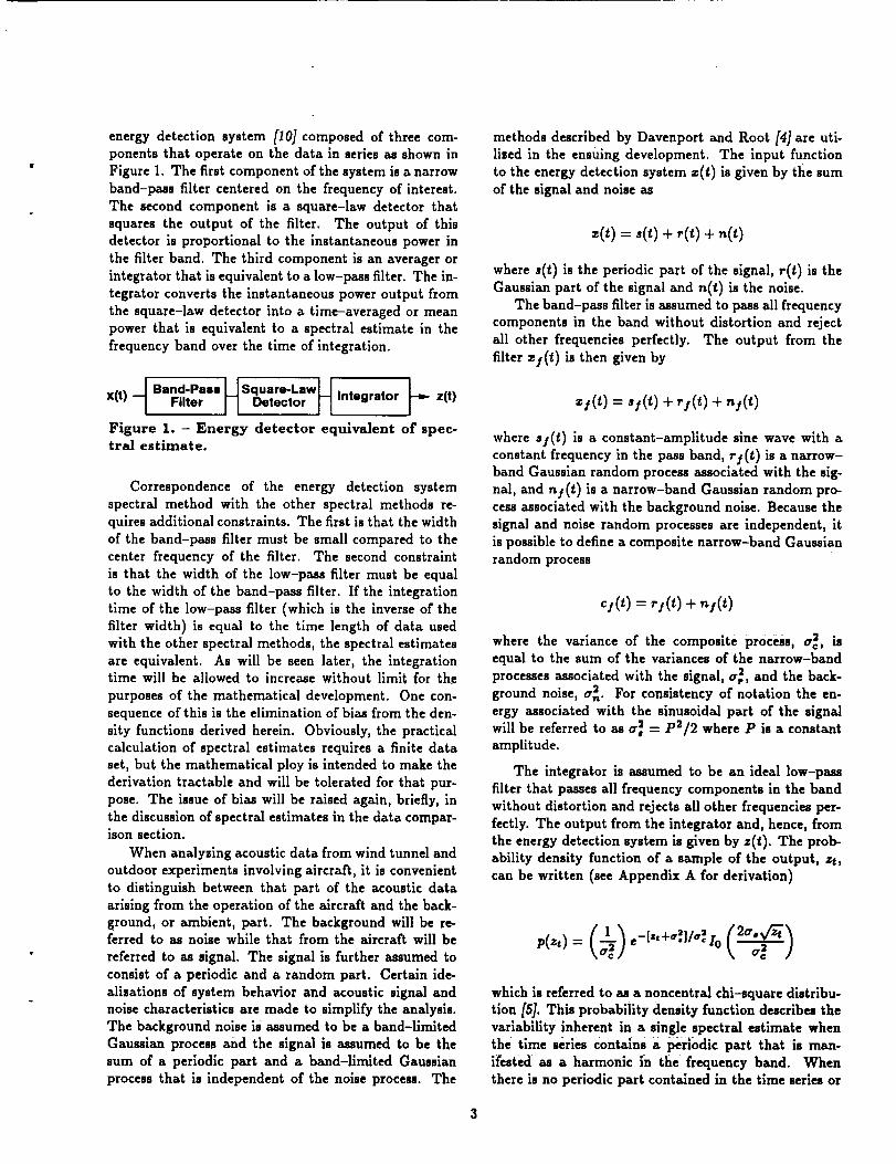
energy detection system [10] composed of three com-ponents that operate on the data in series as shown in

Figure 1. The first component of the system is a narrow

band-pass filter centered on the frequency of interest.

The second component is a square-law detector that

squares the output of the filter. The output of this

detector is proportional to the instantaneous power in

the filter band. The third component is an averager or

integrator that is equivalent to a low-pass filter. The in-

tegrator converts the instantaneous power output from

the square-law detector into a time-averaged or meanpower that is equivalent to a spectral estimate in the

frequency band over the time of integration.

x(t) -_ Band-Pass lJ Square-LawL.]Filter ] J Detector ] [ Integrator _ /(t)

Figure 1. - Energy detector equiva]ent of spec-tral estimate.

Correspondence of the energy detection system

spectral method with the other spectral methods re-quires additional constraints. The first is that the width

of the band-pass filter must be small compared to thecenter frequency of the filter. The second constraint

is that the width of the low-pass filter must be equal

to the width of the band-pass filter. If the integration

time of the low-pass filter (which is the inverse of the

filter width) is equal to the time length of data usedwith the other spectral methods, the spectral estimates

are equivalent. As will be seen later, the integrationtime will be allowed to increase without limit for the

purposes of the mathematical development. One con-

sequence of this is the elimination of bias from the den-

sity functions derived herein. Obviously, the practicalcalculation of spectral estimates requires a finite data

set, but the mathematical ploy is intended to make the

derivation tractable and will be tolerated for that pur-

pose. The issue of bias will be raised again, briefly, inthe discussion of spectral estimates in the data compar-ison section.

When analyzing acoustic data from wind tunnel and

outdoor experiments involving aircraft, it is convenientto distinguish between that part of the acoustic data

arising from the operation of the aircraft and the back-

ground, or ambient, part. The background will be re-ferred to as noise while that from the aircraft will be

referred to as signal. The signal is further assumed to

consist of a periodic and a random part. Certain ide-

alizations of system behavior and acoustic signal and

noise characteristics are made to simplify the analysis.

The background noise is assumed to be a band-limited

Gaussian process and the signal is assumed to be the

sum of a periodic part and a band-limited Gaussianprocess that is independent of the noise process. The

methods described by Davenport and Root [4] are uti-

lised in the ensuing development. The input function

to the energy detection system z(1) is given by the sumof the signal and noise as

"(0 = si0 + + ,,(0

where sit ) is the periodic part of the signal, r(g) is the

Gaussian part of the signal and nit ) is the noise.The band-pass filter is assumed to pass all frequency

components in the band without distortion and reject

all other frequencies perfectly. The output from the

filter z/(1) is then given by

"t(0 = ss( ) + "t(0 + ,*j(0

where s/(t ) is a constant-amplitude sine wave with a

constant frequency in the pass band, _'j(t) is a narrow-band Gaussian random process associated with the sig-

nal, and n! (_) is a narrow-band Gaussian random pro-cess associated with the background noise. Because the

signal and noise random processes are independent, it

is possible to define a composite narrow-band Gaussian

random process

csiO- 'v(O + "l(t)

where the variance of the composite process, cry, isequal to the sum of the variances of the narrow-band

processes associated with the signal, _, and the back-

ground noise, _,_. For consistency of notation the en-

ergy associated with the sinusoidal part of the signal

will be referred to as _ = P2/2 where P is a constantamplitude.

The integrator is assumed to be an ideal low-pass

filter that passes all frequency components in the band

without distortion and rejects all other frequencies per-

fectly. The output from the integrator and, hence, from

the energy detection system is given by z(t). The prob-

ability density function of a sample of the output, zt,

can be written (see Appendix A for derivation)

P(Zd = ( _ ) e-[*'+_3"]/_ l° f 2cr'--v/__\cr_ }

which is referred to as a noncentral chi-square distribu-tion [5].: This probability density function describes the

variability inherent in a single spectral estimate when

the time series contains a periodic part that is man-

ifested as a harmonic in the frequency band. When

there is no periodic part contained in the time series or

when the frequency band under consideration does not

include a harmonic of the periodic signal, the density

function is simply

which is an exponential function or, equivalently, achi-square function of two degree s 0f freedom. These

density functions exactly correspond to results obtained

by Burdic [6] for a matched filter detector in an active

pulse-echo detection system.

When an ensemble of N independent samples of the

detection system output is averaged, the new randomvariable

1 N

/=1

has a probability density function that can be ob-tained by analogy with the results for the multiple pulse

matched filter detector given by Burdic [6] or by coor-dinate transformation of the normalized distribution of

Whalen [5]

N y e_N(_+_:.)#,_IN__\ _rc /

This probability density function describes the variabil-

ity inherent in an ensemble averaged spectral estimate

when the time series contains a periodic part tha t ismanifested _ a harmonicin the frequency band. When

there is no periodic part contained in the time series or

when the frequency band under consideration does not

include a harmonic of the periodic signal, the density

function is simply

which is a chi-square function of 2N degrees of freedom.An interesting feature of this equation is that when

there is no random component of acoustic signal in the

time series, the _ term can simply be replaced by _2n.

Consequently, the origins of the random components ofthe time series, at least insofar as they are Gaussian

and independent, are unimportant to the shape of the

density function. It is also clear that where random

Gaussian components alone are present, their relative

levels are unimportant and the absolute level has no

effect on the relative variability about the mean.

Gaussian Approximation

When the number of spectra included in the averageis large, the Central Limit Theorem can be invoked

[11]. to approximate the noncentral chi-square function

with a Gaussian function. To do this, however, a meanand variance are required. The qth moment of the

noncentral chi-square distribution is given by

g[y ] = f0=

L J x o-o /

where the degenerate hypergeometric function _ is

given by [13].

q,(a, 'y; () = 1 + ( + _- \_--_._..1 +...

The mean of an ensemble average spectral estimate istherefore

which indicates that, as mentioned in the introduction,allowing the integration length to grow without limit

has allowed the derivation of a probability density func-tion tha_ s_o_s no effecl;of the-bfaa-_ssociate_d-w_h-fi-

nite data lengths. The variance of an ensemble averageis given by

= g[:] - u2= +

from which a Gaussian probability density function cannow be written _

p(y) _ --_e-(_-_')_l_'_

that approximates the noncentral chi-square function

for large sample size or when the ratio of periodic

energy to Gaussian energy in the spectral band is great.Two parameters useful for quantifying the deviation of

a statistical distribution from a Gaussian shape and,hence, the applicability of a Gaussian approximationare skewness

2[ 1+3R]*n = _ (I+ 2R)S/aJ

and (excess) Kurtosis

6[ ,+4R1L({

where R 2 2= #,/#c is the ratio of periodic or tonal energy

in the spectral band to the total Oaussian energy (signaland noise) in the band.

By defining a variable that quantifies the relative

variability of a spectral estimate about the expectedvalue

and solving for the lower confidence limit, L, and the

upper confidence limit, U, where W = 1 - 23 is theconfidence coefficient for a two-tailed interval. When

there is no sinusoidal component in a spectral estimate,the density function is chi-square with 2N degrees of

freedom and it can be shown that the limits are given

by L -- $,/N where _ is determined by solving

N-1 _kiT.'k=O

= 2 c#. / l+2RV = _ / #4 + #_ :I/

it is possible to show that when no periodic componentsare present in the time series, then

and U = _/N where _ is determined by solving

N-1 ek

k=O

which serves to reiterate the point made above. When

there is a periodic component to the time series that is

substantially greater than the total random component

the relative variability is approximately

and the relative variability decreases as the ratio of

tonal energy to random energy increases. Clearly, the

relative variability is always less when there is a tonal

component present than when there is not. If the ratio

of tonal energy to Gaussian energy increases withoutbound or if the number of samples in the ensemble av-

erage increases without bound, both skewness and (ex-cess) Kurtosis approach zero and the Gaussian approx-

imation approaches the noncentral chi-square densityfunction

Confidence Limits

The confidence limits of a density function defined

only for positive arguments are determined by integrat-ing under the tails

and either

or_o U1 - 3 = v( )ay

The expected value of the normalized density function

for noise only is just unity and the variance is givenby 1/I'I. When a sinusoidal component is present in

a spectral estimate, the density function is noncentral

chi-square with 2N degrees of freedom and numericalintegration must be performed. The details of the

numerical integration scheme are given in AppendixB. Solving for the upper and lower confidence limits

involves finding the root of each of the integrations.The numerical methods used for this process are also

detailed in Appendix B.

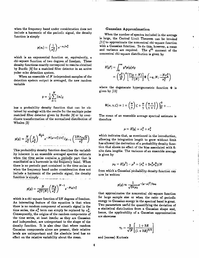
A comparison of the noncentral chi-square, X_,and chi-square, X02, distributions is shown in Pigure 2below. For this example, both distributions have four

degrees of freedom because they describe an averageof two spectra. Both distributions have the same

mean (or total energy) but the ratio of tonal energy

to broadband energy is R = 10 (or 10 dB) for thenoncentral distribution. The horizontal scale of the

plot is normalized by the noise energy of the noncentral

distribution so the total energy of both distributions is

given by 1 + R. The noncentral distribution, denotedby the solid line, is noticably narrower than the central

distribution, denoted by the dashed line.

The upper and lower 80% confidence limits, ex-

pressed in decibels, are asymmetrically spaced becauseof both the decibel scale and the asymmetry of the dis-tributions. The plot shows there is an 80% confidence

that the actual spectral level is no more than 1.43 dBabove and no more than 1.94 dB below the estimated

level when the tone-to-noise ratio is 10 dB in the spec-tral band. This compares with an 80% confidence in-

terval from 2.89 dB above to 5.75 dB below an estimate

in a spectral band containing only broadband noise. As

the tone-to-noise ratio approaches sero the shape of

the noncentral chi-square distribution approaches the

shape of the chi-square distribution. As the tone-to-noise ratio increases the noncentral chi-square distri-

bution becomes narrower and the confidence limits ap-proach the estimated spectral level.

Number of Spectra: 2

Tone-to- Noise Ratio: I0.00 dB

Confidence Coefficient: 80.00

-- Xt z, Upper LimH: 1.43 dE

.10 - XRz, Lower Limit: -1,94 dE

"-- Xo=, Upper Limit: 2.89 dB_" Xo, Lower Limit: -5.75 dS

rt J ._

-y ",,, \ i

O. 0 10 20 30 40 50

Z

Figure 2. - Comparison of noncentral chl-

square, X_, and chi-square, X_, distributions.

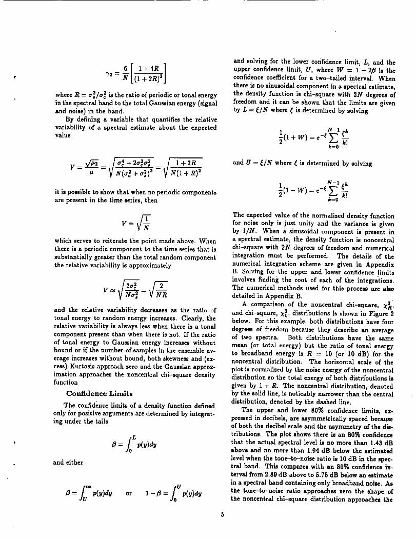
A comparison of the noncentral chi-square distribu-

tion, X_, and a Gaussian approximation is shown inFigure 3 below. The noncentral chi-square distribution

again has four degrees of freedom because it describes

an average of two spectra. The tone-to-noise ratio is5 dB so R _, 3.16. The Gaussian distribution has the

same mean (or total energy) as the noncentral distribu-tion. The horizontal scale of the plot is again normal-ized by the noise energy of the noncentral distribution

so the total energy of both distributions is again givenby 1 + R. The variance of the Gaussian distribution is

given by (1 + 2R)/N. The noncentral distribution, de-noted by the solid line, is noticably more skewed than

the Gaussian distribution, denoted by the dashed line,

which is symmetric.

.25 ' ' ' _ I ' _ ' ' I ' * ' ' l ' ' ' '

Number of Spectra: 2

Tone-to-Noise Ratio: 5.00 HB

.20 / ,"'_" Confidence Coefflclenh 99,90 _;

/ ' _ "_ -- Xa z, Upper Lira;i: 4,86 dB

// \\ X,z, Low.rLimlt: -11.84dB

.15 // \', --- Gousslon Upper Limit: 4.00dB

,'_ 1/ \',, Co...,onLo,,.erLira.:

a. , ,.10 , ,

.05

o.o_L.x ..... I , ,,-'_-.'L'C--L_ l, , I , , , ,5 10 15 20

Z

Figure 3. - Comparison of noncentral chi-

square, X._, and Gaussian distributions.

m

o

.r-

E°m

4DO¢-4D

"10oD

t-O

O

The plot shows there is 99.9% confidence that the

actual spectral level is no more than 4.86 dB above and

no more than 11.84 dB below the estimated level when

the tone-to-noise ratio is 5 dB in the spectral band.

The Gaussian distribution has an upper 99.9% confi-dence limit of 4 dB but an undefined lower confidence

limit because the lower tail of the curve extends below

zero. As either the tone-to-noise ratio or the number of

spectra increases the Gaussian distribution more closelyapproximates the noncentral chi-square.

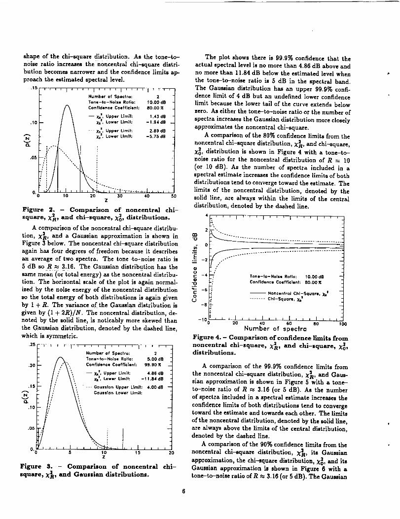
A comparison of the 80% confidence limits from the

noncentral chi-square distribution, X_, and chi-square,X02, distribution is shown in Figure 4 with a tone-to-

noise ratio for the noncentral distribution of R = 10

(or 10 dB). As the number of spectra included in aspectral estimate increases the confidence limits of both

distributions tend to converge toward the estimate. The

limits of the noncentral distribution, denoted by thesolid line, are always within the limits of the centraldistribution, denoted by the dashed line.

4

2

0

-2

-4

coo,,o.::.oo.:,,:,::,::o.oo,.:-6 _ _No_c.ontral Chl;Square. Xa= ---

- I 00 20 40 60 so _coNumber of spectra

Figure 4. - Comparison of confidence limits from

noneentral chi-square, X_, and chi-square, X0z,distributions.

A comparison of the 99.9% confidence limits from

the noncentral chi-square distribution, X_, and Gaus-sian approximation is shown in Figure 5 with a tone-

to-noise ratio of R _ 3.16 (or 5 dB). As the numberof spectra included in a spectral estimate increases the

confidence limits of both distributions tend to convergetoward the estimate and towards each other. The limits

of the noncentral distribution, denoted by the solid line,

are always above the limits of the central distribution,denoted by the dashed line.

A comparison of the 90% confidence limits from the

noncentral chi-square distribution, X_, its Gaussian

approximation, the chi-square distribution, )Ca, and itsGaussian approximation is shown in Figure 6 with a

tone-to-noise ratio of R _. 3.16 (or 5 dB). The Gaussian

6

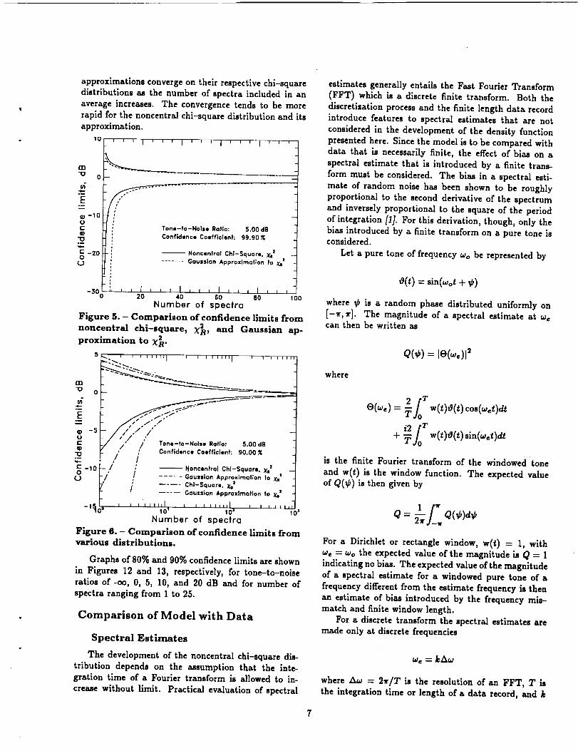
approximations converge on their respective chi-squaredistributions as the number of spectra included in an

average increases. The convergence tends to be more

rapid for the noncentral chi-square distribution and itsapproximation.

10 '''r

_ 0 -

E-- j,

-I0 lOE

E -20o i

El

-U 0

d

B

-5OE

"13

C -100

¢J

' ' ' I ' ' ' I ' ' ' t ' ' '

Tone-to-Noise Ratio: 5.00 dB

Confidence Coefflclont: 99.90 g

Noncenlrol ChI-Square, Xt=

....... Gaussian Approximation !o X_=

_300 h , , I , r , l , , , I , i I l20 40 SO 80

Number of spectra

I I

100

Figure 5. - Comparison of confidence limits from

noneentral chi-square, X_, and Gaussian ap-

proximation to X_-

,_I I l I I llllJ I I I l llllJ I 1_a,,.+ -_ J

/,/ .,

/" / Tone-to-Noise Ratio: 5.00 dS' : Confidence Coefficient: 90.00 _{

,/ // ; -- Noncenlrol Chl-$quaro, X. z

/ ..... Gousslon Approximolion to Xm=/'

] .... Chl-Squore, Xoa

.... Goussian Approximation to Xo=

--1_1 J J _ i JlllJ10 w I I I i J,,,Jlo z i i i ],_LtG

Number of spectra

Figure 6. - Comparison of confidence limits fromvarious distributions.

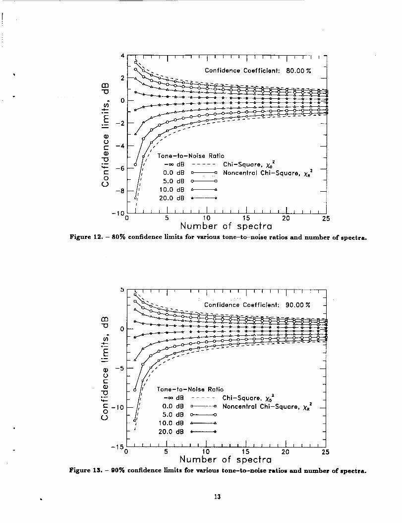
Graphs of 80% and 90% confidence limits are shown

in Figures 12 and 13, respectively, for tone-to-noise

ratios of-co, 0, 5, 10, and 20 dB and for number of

spectra ranging from 1 to 25.

Comparison of Model with Data

Spectral Estimates

The development of the noncentral chi-square dis-

tribution depends on the assumption that the inte-gration time of a Fourier transform is allowed to in-

crease without limit. Practical evaluation of spectral

estimates generally entails the Fast Fourier Transform(FFT) which is a discrete finite transform. Both the

discretization process and the finite length data recordintroduce features to spectral estimates that are not

considered in the development of the density function

presented here. Since the model is to be compared withdata that is necessarily finite, the effect of bias on a

spectral estimate that is introduced by a finite trans-

form must be considered. The bias in a spectral esti-

mate of random noise has been shown to be roughlyproportional to the second derivative of the spectrum

and inversely proportional to the square of the period

of integration [1]. For this derivation, though, only the

bias introduced by a finite transform on a pure tone isconsidered.

Let a pure tone of frequency Wo be represented by

O(t) = sin(wot + _b)

where ¢ is a random phase distributed uniformly on[-_r,_r}. The magnitude of a spectral estimate at wecan then be written as

Q(W)= IO( e)l2

where

2/;= w(t) (t)cos( eOdt

i2_IT w(_),_(_)sin(_et)dt+ TJo

is the finite Fourier transform of the windowed tone

and w(t) is the window function. The expected valueof Q(¢) is then given by

1 f'w

Q = Q(¢)d¢

For a Dirichlet or rectangle window, w(t) = 1, with

ate = wo the expected value of the magnitude is Q = 1

indicating no bias. The expected value of the magnitudeof a spectral estimate for a windowed pure tone of a

frequency different from the estimate frequency is thenan estimate of bias introduced by the frequency mis-match and finite window length.

For a discrete transform the spectral estimates are

made only at discrete frequencies

+.,, = kAw

where A_a = 27c/T is the resolution of an FFT, T is

the integration time or length of a data record, and k

is a frequency index. The tone frequency may then bespecified as

.,o = (k+ Aw

where k is the index that refers to the discrete frequency

nearest the tone frequency and e = (wo- we)/Aw isan indicial measure of the difference between tone and

estimate frequencies such that

1 1--<¢< -

2- -2

A number of common window functions [12] may berepresented by

w(0 = wo - Wlcos(Aw )+ w2 cos (2Awt)

- ws cos (3Awt)

where various choices for the coefficients wl define par-ticular windows. The coefficients may be chosen so thatthe window is power preserving insofar as the total en-

ergy or mean power of a spectral estimate of a random

process is unbiased on the average

w'(t)dt : 1

Coefficients of a number of window functions of this

type [I2] expressed in a power preserving form areshown in Table 1 below.

Table I. - Coefficients of selected windows.

Window w0 wl w 2 wa

Dirichlet 1,0000 0.0 0.0 0.0

Hanning 0.8165 0.8165 0.0 0.0

Hamming 0.8566 0.7297 0.0 0.0

Blackman 0.7610 0.9060 0.1450 0.0

Kaiser-Bessel 0.7463 0.9236 0.1823

4-sample, a = 3

0.0226

Blackman-Harris 0.7063 0.9614 0.2782 0.0230

min 4-sample

The bias correction may now be written in terms of

the window coefficients, wl, estimate frequency index,k, and mis-match index, ¢, as

with

Q = sinc_ (Tre) ( F2 +2 G2)

and

2k + 2_'_F = w0 Tk

G= wo +_H-

Hi=-wl _+(2k+_)a_l

+ w_ + (2k +_)2 _ 4

- w._ + (2k + _)2 _ 9

For the case where the tone frequency and estimate

frequency are the same, We = Wo or • = 0, a window

introduces some bias with the correction given, forexample, by

201oglo[Q]= 201og10[w0]

-1.76 dB for Hanning

-1.34 dB for Hamming

In other words, the discrete finite transform spectralestimate of a pure tone with a frequency other than one

of the discrete estimate frequencies will exhibit a peak

lower then the magnitude of the tonal energy (bias)and will show the remaining energy from that tonespread across every discrete frequency of the estimate

(leakage). The value Q gives the fraction of the originaltonal energy that resides in the frequency bin we nearest

the tone frequency wo. This fraction of the originaltonal energy that remains in the spectral frequency bin

is the value that should be used for the energy of the

tonal signal, Q_r_ rather than o,_, in calculating thedensity function and evaluating confidence limits.

The bias correction may be made for any arbitrarysymmetric window in the same manner. The window

correction component H:E may be expressed as

where the window coefficients, wl, are determined bydiscrete Fourier transform of the window.

Synthesized Data

Synthesized data were used to verify the mathemat-

ical form of the noncentral chi-square density function

and the numerical methods employed in its evaluation.

Data records were constructed by adding white noiseto sine waves. Each value of white noise for each data

record was generated as an independent sample from a

standard normal distribution by a commercial pseudo-

random number generator and then scaled to the ap-propriate absolute level. The phase of the sine wave

for each data record was generated as an independent

sample from a uniform distribution on the interval C0,1)

by a commercial pseudorandom number generator and

then transformed to the interval (-Tr, _r). Each datarecord was transformed by an FFT after a window was

applied and the squared magnitude was then calculated

to generate a spectral record. A spectral average wasdetermined from the appropriate number of spectralrecords and the resulting spectral estimate at the fre-

quency of interest was recorded for statistical analysis.

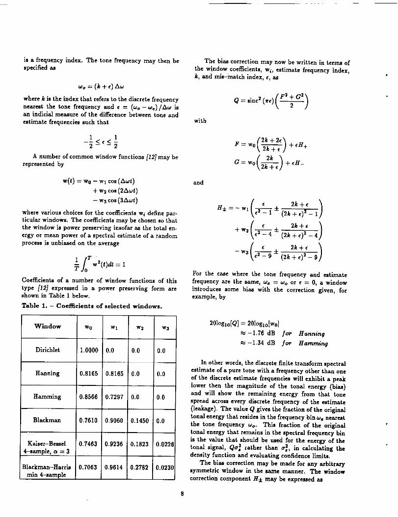
s.0 ' I ' I ' I ' t ' I ' I ' I ' I ' JN " Tone Level: 70.00 dg ]

C 7.0 - Tone Frequency: 20,00 Hz -'1

>" " No;se Level: 59.90 dE j"[3

s.O - r_ stzs: 2og8 •1: " R..ol-,O.: ,.,gH_ 1O 5.0 - _ Wlndow: g-sample Kolser-Besssl-

" - _ Spectra: 2 -t-

O.O- /\ o_o. ,ooo_3.0

2,0 - _ .AI "',, -- S_os.d _

g l.O

O.o.];_, I.-r'"i , 1 , I_'_4--_ L, "]'"i"'| ......lo .20 .so .go .50 so ,7o .so .9oSPL. dyne2/cm 4

Figure 7. - Comparison of biased and unbiasednoncentral ehi-square distributions with an es-

timate obtained from synthesised data.

The results from one realization of this process are

shown in Figure 7 above. A pure tone of 20 Hzata level of 70 dB was added to noise at a level of 90

dB. The sample rate was 2344 per second so a data

record size of 2048 points gave a resolution of about

1.14 Hz and yielded an average noise level of about 60

dB in each frequency band. A 4-sample Kaiser-Bessel

ice = 3) window was used, two--record spectral averages

were calculated, and 1000 estimates at the frequencyband nearest the tone, 19.457 Hz, were recorded. The

histogram shows the approximate density function esti-mated from the synthesized data. The smooth curve

shown by the solid line is the noncentral chi-squaredensity function where the window bias correction was

made. The smooth curve shown by the dashed line

is the noncentral chi-square 'density function where nowindow bias correction was made.

The bias corrected theoretical curve agrees very wellwith the histogram estimate from synthesized data. A

parametric evaluation of the agreement between the-ory and synthesized data is summarized in Table 2 be-

low. The parameters of interest, mean, standard devi-

ation, skewness, and (excess) Kurtosis, are listed in thefirst column. The values for those parameters estimated

from the distribution of spectral estimates are listed in

the second column. The corresponding bias corrected

theoretical parameters appear in the third column. The

t statistic in the fourth column is for testing the null hy-pothesis that the estimated and theoretical parametersare equal. The critical value at the 50% level for 1000

samples is t.s0[s0s] = .6744 so the null hypothesis is notrejected for either the mean or the standard deviation.

The critical value at the 50% level for infinite degrees of

freedom is t.s0[oo ] : .6742 so the null hypothesis is also

not rejected for either the skewness or (excess) Kurtosis.

Table 2. - Selected parameters of biased noneen-

tral ehi-square distribution.

Parameter

Mean

Std. Dev.

Skewness

Kurtosis

Estimate

0.2182

0.08890.6224

0.4545

Theory t statistic0.2193 -.3791

0.0883 0.29100.6417 -.2495

0.5580 -.6698

Given the conflicting assumptions necessary to de-

rive the model and correct for bias, as well as limitations

imposed by the random number generator and the useof a discrete transform, it would seem that the non-

central chi-square distribution appropriately describes

the distribution of spectral estimates for a pure tone inGaussian noise and that the numerical evaluation of the

distribution is accurately accomplished.

Tiltrotor Hover Data

Acoustic data acquired during an XV-15 tiltrotor

hover test were obtained to evaluate the applicability

of the noncentral chi-square distribution to helicopterspectral estimates. Data from a single channel were

converted to engineering units and spectra were calcu-

lated from sequential segments of data with no overlapin the same manner as the synthesized data. Spectral

averageswere determined from the appropriate numberof spectral records and the resulting spectral estimate

at the frequency of greatest magnitude was recorded forstatistical analysis.

Because the noise level and tone level were not

known a priori, they were estimated from the spectra.

The sample rate for these data was 24590 per secondso a data record size of 8192 gave a resolution of about

3 Hz. A 4-sample Kaiser-Bessel (a = 3) window wasused, two-record spectral averages were calculated, and44 estimates were made from the limited amount of data

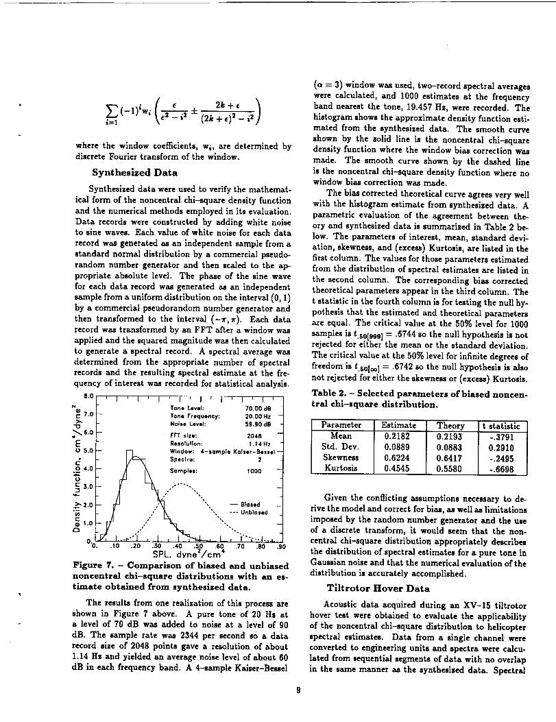
available. An average spectrum of all the estimates is

shown in Figure 8 below. The solid line is the averageof all of the spectra while the dashed lines describe

the envelope containing the 44 spectral averages of two

spectra each. The peak spectral level occurs at 27.02Hs and the background noise per band was estimated

from the spectral average curve to be about 56 dB at

that frequency. The tone level in that frequency band

was then found by subtracting the noise energy in the

band from the total energy in the band. No correctionwas made for bias because the spectral levels used for

this calculation were already biased.

tO0| j , , , I

-- Average

--- _'nvelope

9°r-t

J'Om 80-- I

(i.

U') 70 _60

ipi

50"" ' (o

, /

e

50

[stlmated Tone Level: 90.6

Estimated Frequency: 27.02 Hz I

Estimated Noise Level: 56.00 dB --I/

FFT size: 8192 |

Resolution: `3,00 Hz

Window: 4-sample Kalser-Ressel

Spectra: 2

_Sarnples: 44

L _ II i o

1O0 150 200

Frequency, Hz

Figure 8. - XV-15 tUtrotor spectral average and

envelope of spectra comprising the average.

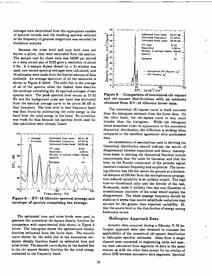
The estimated tone and noise levels were used to

generate the noncentrai chi-square density function for

comparison with experimental data shown in Figure 9below. The histogram shows the approximate densityfunction estimated from the hover data. The smooth

curve shown by the solid line is the noncentral chi-

square density function based on estimated tone and

noise levels. The smooth curve shown by the dashed line

is the chi-square density function for the total energy

contained in the frequency band.

,50 z , j

_=).45C

-0_.4o

0.30

_.25

_ .20

'*-.15

O. 0

t I I I l t t I I

Estimated Tone Level: 90.61 dB --

Estimated Frequency: 27.02 Hz

Estimated Noise Level: 56.00 dB --

FF"T size: 8192 -Resolution: ,3.00 Hz

Window: 4-sample Kalsor-Bessel "

Spectra: 2

Samples: 44

-- Noncentral Chi-Square. X. z .._

--- Chi-Squaro. X¢ z

"- -I-----f_--d._. J. --,L_= __ J.__ l | l

50 I O0 150

SPL. dvne2/cm 4

Figure g. - Comparison ofnoncentraI chi-squareand ehi-square distributions with an estimate

obtained from XV-15 tiltrotor hover data.

The noncentral chi-square curve is much narrowerthan the histogram estimate from the hover data. On

the other hand, the chi-square curve is very much

broader than the histogram. While the histogramseems somewhat closer in appearance to the noncentral

theoretical distribution, the difference is striking when

compared to the excellent agreement with synthesiseddata.

An examination of assumptions used in deriving thetheoretical distribution should indicate the source of

disagreement between experiment and theory. Assump-tions made in deriving the theoretical function includerequirements that the noise be Gaussian and that the

tone, or the Fourier component of the periodic signal,

maintain constant frequency and amplitude. The hover-

ing tiltrotor was 100 feet above the ground at a horison-

tal distance of 500 feet from the microphone so propaga-

tion induced variability is an unlikely culprit. The high

tone-to-broadband ratio and the brevity of the test,30 seconds, make it unlikely that any non-Gaussian or

nonstationary character of the noise would explain the

disagreement. The blade passage frequency should be

stable so it seems that source amplitude variations may

account for the greater than expected variability. Ei-

ther the source level or the distribution of energy amongharmonics varied.

Helicopter Approach Data

Acoustic data acquired during a Sikorsky S-76 he-licopter approach were also obtained to evaluate the

applicability of the noncentral chi-square distribution

to helicopter spectral estimates. Data from a single

channel were converted to engineering units and spec-tra were calculated from segments of data in the same

manner as with the other data except for an overlap ofabout 35% between successive data segments. Spectral

10

overlapping was used to get as many independent esti-

mates as possible in a short time interval. Harris [12].has suggested that transforms with this level of over-

lap are essentially independent when good windows are

used. Spectral averages were determined from the ap-

p/0priate number of spectral records and the resulting

spectral estimate at the frequency of the second blade

passage harmonic was recorded for statistical analysis.Because the noise level and tone level were not

known a priori, they were estimated from the spectra.The sample rate for these data was 2344 per second so a

data record size of 2048 gave a resolution of about 1.14

Hs. A 4-sample Kaiser-Bessel (c_ = 3) window wasused, three-record spectral averages were calculated,and 35 estimates were made from a small fraction of

the available data. The helicopter was approaching at

a constant speed so the range was constantly shrinking

and the tone level constantly increasing. The datawere selected from a fairly short time interval at a

relatively long range to minimize the relative effect

of the changing range yet give sufficient data for ahistogram estimate of the density function.

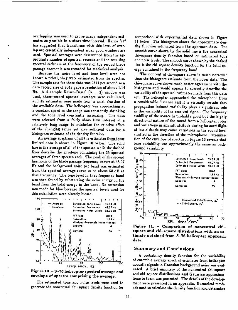
An average spectrum of all the estimates from these

limited data is shown in Figure 10 below. The solid

line is the average of all of the spectra while the dashed

lines describe the envelope containing the 35 spectral

averages of three spectra each. The peak of the secondharmonic of the blade passage frequency occurs at 48.07

Hz and the background noise per band was estimated

from the spectral average curve to be about 58 dB at

that frequency. The tone level in that frequency band

was then found by subtracting the noise energy in theband from the total energy in the band. No correction

was made for bias because the spectral levels used forthis calculation were already biased.

tlO , , _ , [ J _ t _ l r _ _ _ [ j i--w J 1

--Average Estimated Tons Level: 85.04 dB

tO0 =- --- Envelope Estimated Frequency: 48.07Hz _j

Eslimaforl Noise Level: 58.00 dR J

FF'F slze: 2048 ]' Resolution: 1.14 Hz --1

SO _' Window: 4-sample Kalssr-Bessol ii=

i _ Spectra: 3 "

q

- 80 ; l.[ _, Samples: 35',I s, :i

i,, J_ ,

' h /",

SO " , ' "" ',' " ' , I.. ,, , _,;,, , , ,.'_,,.'_'_ ,, _ _* _ . , ,_,

, , _ ., ,,.,,, , ¢,.:,.,: -,_.,, :,,..,,500 ;A_'v,_,.:t-;i v_,,,x, ,AI^ _ ,,, ,v',:..

50 I00 t 50 200

Frequency, Hz

Figure 10. - 5-?6 helicopter spectral average and

envelope of spectra comprising the average.

The estimated tone and noise levels were used to

generate the noncentral chi-square density function for

comparison with experimental data shown in Figure11 below. The histogram shows the approximate den-sity function estimated from the approach data. The

smooth curve shown by the solid line is the noncentral

chi-square density function based on estimated tone

and noise levels. The smooth curve shown by the dashedline is the chi-square density function for the total en-

ergy contained in the frequency band.

The noncentral chi-square curve is much narrowerthan the histogram estimate from the hover data. The

chi-square curve shows much better agreement with thehistogram and would appear to correctly describe the

variability of the spectral estimates made from this data

set. The helicopter approached the microphone from

a considerable distance and it is virtually certain that

propagation induced variability plays a significant role

in the variability of the received signal. The frequency

stability of the source is probably good but the highly

directional nature of the sound from a helicopter rotor

and variations in aircraft attitude during forward flightat low altitude may cause variations in the sound level

emitted in the direction of the microphone. Examina-

tion of the envelope of spectra in Figure 10 reveals thattone variability was approximately the same as back-ground variability.

.90 ' I Il

.80 -

.70 -

E.6o -U .

_.50 --O "

"_ .40 --

C "

,_3.30 -

_ .20 -VI

1-

• '.10 -

0"0 10

l I I I I ' I ' I _-Estimated Tons Level: 85.04 dE --Estimated Frequency: 48.07 Hz

Estimated Noise Level: 58.00 dg --

FFT size: 2048

Resolution: 1.14 Hz --

Window: 4-sample Kalssr-Bssssl

Spectra: ,3 --

Samples: 35 .__

-- Noncentral Chi-Squars, Xe z "--- Chi-5quaro. Xo=

_"FFI---,-,-,:'__ , .-1 , _l , [ I20 30 40 50 60 70

SPL. dyne2/cm 4

Figure 11. - Comparison of noncentral ehi-

square and chi-square distributions with an es-

timate obtained from S-76 helicopter approachdata.

Summary and Conclusions

A probability density function for the variability

of ensemble average spectral estimates from helicopteracoustic signals in Gauuian background noise was eval-

uated. A brief summary of the noncentral chi-Kluare

and chi-square distributions and Gaussian approxima-

tions to them was presented. The details of the develop-

ment were presented in an appendix. Numerical meth-ods used to calculate the density function and determine

11

confidence limits were presented in another appendix.

A FORTRAN program that implements the numerical

methods to calculate confidence limits also appears inan appendix.

Examples were plotted to show differences and sim-

ilarities between the density functions. Plots were also

presented to show differences between confidence lim-

its versus the number of spectra included in an averagefor various confidence coefficients and tone-to-noise ra-

tios. The noncentral chi-square density function was

then compared with synthesized data that closely ap-

proximated assumptions made in development of the

model, with short range tiltrotor hover data, and with

very long range helicopter approach data.

The excellent agreement between synthesized dataand theoretical curves indicates that the numerical

methods and computer program worked as desired. Thesomewhat poorer agreement between the tiltrotor hover

data and theoretical curves is likely an indication thatthe assumption of constant source level was violated. In

this case the noncentral chi-square distribution was im-

perfect but showed better agreement with the data than

the chi-square distribution. The data from a helicopter

approaching an observer showed very poor agreementwith the noncentral chi-square distribution. The much

better agreement of this data with the chi-square den-

sity function is an indication that extremely variable

tone levels, whether from source variability or propaga-tion effects, completely invalidate the use of the noncen-

tral chi-square distribution. The noncentral chi-square

distribution should give excellent agreement, however,

over time scales where the tone levels do not vary sig-nificantly, as in wind tunnel measured acoustic data.

Acknowledgements

The author would like to thank Charlie Smith for

providing the S-76 helicopter approach data that was

used to calculate spectra for comparison with the non-central chi-square density function. He would also like

to thank Ken Rutledge for providing the XV-15 hover

data that was used for the same purpose, and for his

suggestions for improving this work.

References

1. Hardin, Jay C.: Introduction to Time Series

Analysis. NASA RP-1145, March 1986.

2. Bendat, Julius S. and Piersol, Allan G.: Random

Data: Analysis and Measurement Procedures, SecondEd. John Wiley & Sons, Inc., 1988.

3. Rutledge, Charles K.: On the Appropriateness

of Applying Chi-Square Distribution Based Confidence

Intervals to Spectral Estimates of Helicopter FlyoverData. NASA CR-181692, August 1988.

4. Davenport, Wilbur B., Jr. and Root, William L.:

An Introduction to the Theo_T o/Random Signals andNoise. McGraw-Hill Book Co., Inc., 1958.

5. Whalen, Anthony D.: Detection o/Signals inNoise Academic Press, Inc., 1971.

6. Burdic, William S.: Underwater Acoustic SystemAnalysis. Prentice-Hall, Inc., 1984.

7. Rice, S. O.: Statistical Froperties of a Sine Wave

Flus Random Noise. Bell Syst. Tech. Jour., Vol. 27,1948.

8. Reich, Edgar and Swerling, Peter: The Detection

o/a Sine Ware in Gaassian Noise. Journal of AppliedPhysics, Vol. 24, No. 3, March, 1953.

9. Hinich, Melvin J.: Detecting a Hidden Peri-odic Signal When Its Period is Unknown. IEEE Trans-

actions on Acoustics, Speech, and Signal Processing,Vol. ASSP-30, No. 5, October 1982.

10. Urick, Robert J.: Principles of Underloater

Sound, Third Ed. McGraw-Hill Book Co., Inc., 1983.11. Hoel, Paul G.: Introduction to Mathematical

Statistics, Fourth Ed. John Wiley & Sons, Inc., 1971.

12. Harris, F. J.: On the Use of Windows/or Har-monic Analysis with the Discrete Fourier _'anaform.

Proc. of the IEEE, Vol. 66, No. 1, 1978.

13. Gradshteyn, Izrail. S. and Ryshik, Iosif. M.:

Table of Integrals, Series, and FroducLg, Corrected and

Enlarged Ed. Academic Press, Inc., 1980.

14. Abramowits, Milton and Stegun, Irene A.:Handbook o/Mathematical Functions. Dover Publica-tions, Inc., 1970.

15. Davis, Philip J. and Rabinowits, Philip: Meth-ods of Numerical Integration, Second Ed. Academic

Press, Inc., 1984.

12

I

nn-0

c

C0

4

2

0

-2

-4

-6

-8

-100

I''''1''''1

Confidence Coefficient: 80.00%

I

i I

I

/

I

/

Tone-to-Noise Ratio

-co dB ..... Chi-Squore, X0=

0.0 dB _ Noncenfrol Chi-Squore, XR=5.0 dB o_o

10.0 dB

20.0 dB

5 10 15 20

Number of spectra25

Figure 12. - 80% confidence limits for various tone-to-nolse ratios and number o£ spectra.

I ,,,I,l,,I

Confidence Coefficient: 90.00_=

rn-0

amw

uc

-04--

C0

C_

Tone-to-Noise Ratio

-oo dB Chi-Square, X0z

0.0 dB --------- Noncentral Chi-Squore, XRz5.0 dB

10.0 dB

20.0 dB = _-

-150 5 10 15 20 25

Number of spectra

Figure 13. - 90% confidence limits for various tone-to-noise ratios and number of spectra.

, 13

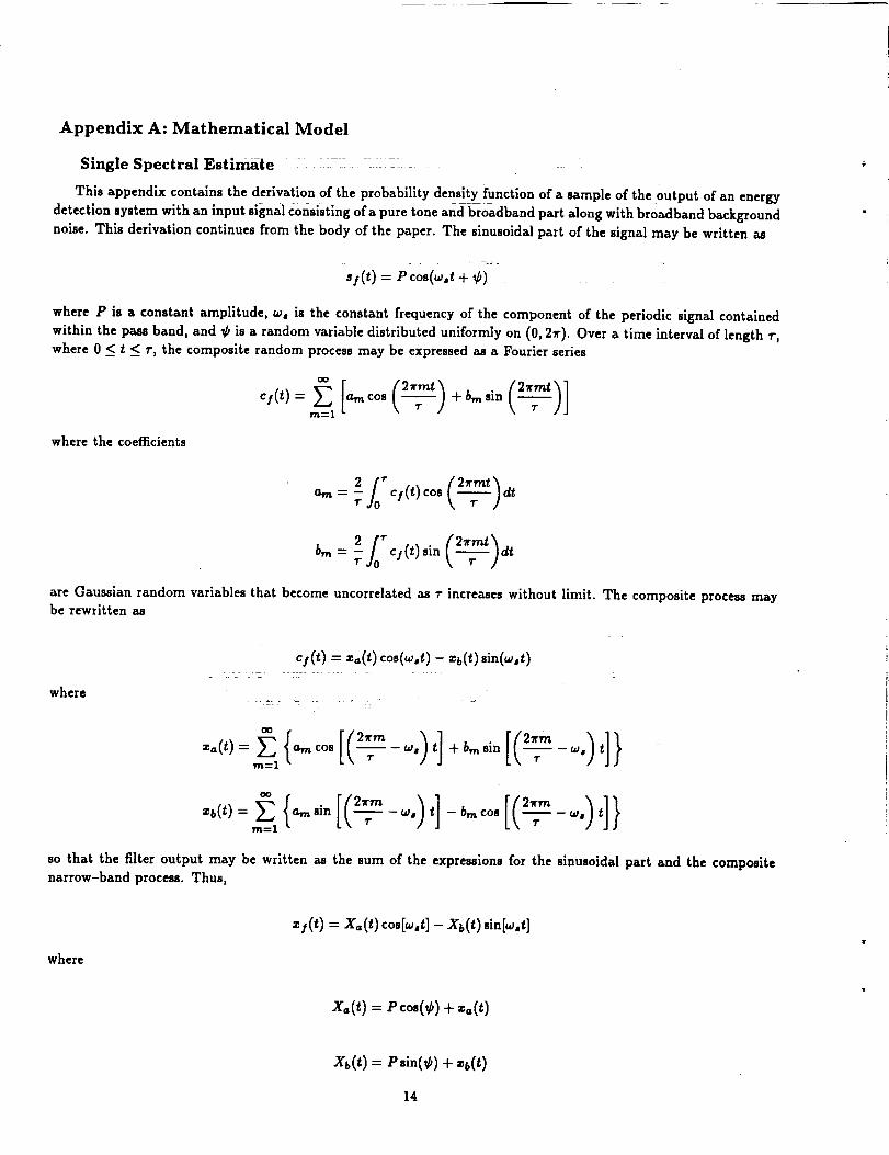
Appendix A: Mathematical Model

Single Spectral Estimate

This appendix contains the derivation of the probability density function of a sample of the output of an energy

detection system with an input signal Consisting of a pure _bneandbroadband part along with broadband background

noise. This derivation continues from the body of the paper. The sinusoidal part of the signal may be written as

where P is a constant amplitude, wj is the constant frequency of the component of the periodic signal contained

within the pass band, and ¢ is a random variable distributed uniformly on (0, 2x). Over a time interval of length _',where 0 < t < r, the composite random process may be expressed as a Fourier series

oo

where the coefficients

am=- c/(t)cos _2 t dtT

'/:bm= r e/(t)sin dt

are Gaussian random variables that become uncorrelated as 7"increases without limit. The composite process maybe rewritten as

where

cl(t) = za(t)cos(w,t)- zb(t)sin(w,t)

Oo

m=1 I"

so that the filter Output may be written as the sum of the expressions for the sinusoidal part and the compositenarrow-band process. Thus,

where

z/(t) = X_(t) cos[a,,t] - Xb(t) sin[wot]

xo(t)= Pcos(¢)+ ..(t)

Xb(t) : Psin(_b) + Zb(t )

14

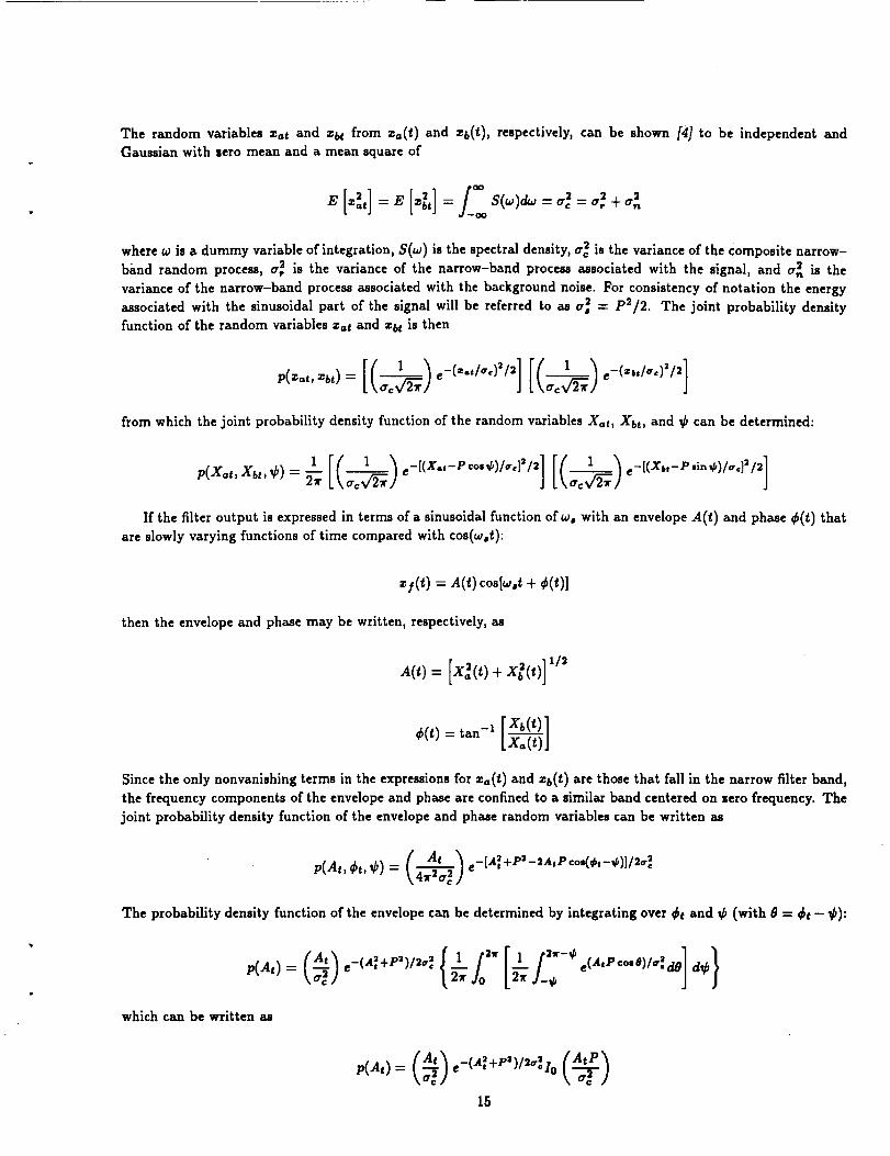
The random variables zat and zs¢ from za(t) and zs(_), respectively, can be shown [4] to be independent and

Gaussian with sero mean and a mean square of

where w is a dummy variable of integration, S(a_) is the spectral density, cr_ is the variance of the Composite narrow-

band random process, 0,_ is the variance of the narrow-band process associated with the signal, and cv_ is the

variance of the narrow-band process associated with the background noise. For consistency of notation the energy

associated with the sinusoidal part of the signal will be referred to as c,_ = P_/2. The joint probability density

function of the random variables zat and zbt is then

from which the joint probability density function of the random variables Xat, Xb,, and _b can be determined:

]If the filter output is expressed in terms of a sinusoidal function ofaJ, with an envelope A(t) and phase _(t) that

are slowly varying functions of time compared with cos(_,t):

then the envelope and phase may be written, respectively, as

A(f,) = [.X_(f,)q'- .X/_(I_)] 1/2

= tan-1LX.,(t)J

Since the only nonvanishing terms in the expressions for za(t) and Zb(t ) are those that fall in the narrow filter band,

the frequency components of the envelope and phase are confined to a similar band centered on zero frequency. The

joint probability density function of the envelope and phase random variables can be written as

At

p(Atl Otl _b) =14-'_2c l e-[A31+PI-2AIP c°I(@I-@)]II¢_

The probability density function of the envelope can be determined by integrating over _t and ¢ (with 0 = _t - @):

which can be written as

A,,) e_(A_+P,)l.ja._i ° f AtP_

15

where I00 is the zero-order modified Bessel function.

The output from the square-law detector is

• 3(t) = A_(0cos:%._+ ¢,(t)]= _a"(t)+ _A'(t)cosC2b.'._+ ¢'(0])

The integrator is assumed to be an ideal low-pass filter that passes all frequency components in the band without

distortion and rejects all other frequencies perfectly. The low-pass filter width is the same as the band-pass filter

width so that the square of the envelope function, with all its frequency components in the pass band, is passed

by the integrator. The high-frequency component of the square-law detector output, with a frequency of 2w,, is

rejected •because the band-pass filter width must be small compared with Wo to satisfy the assumption that c/(t)is a narrow-band Gaussian random process. The output from the integrator and, hence, from the energy detection

system is given by z(t) where

The probability density function of zt can be obtained by a simple transformation to give an expression

k _ J

which is referred to as a noncentral chi-square distribution [5]. This is the probability density function that describes

the variability inherent in a single spectral estimate when the time series contains a periodic part that is manifested

as a harmonic in the frequency band.

16

Appendix B: Numerical Methods

Density Function Evaluation

Although the density functions appear to be relatively clear and concise, their numerical evaluation is difficult.

When there is no periodic signal present the density function is the product of a constant, a power, and an exponential.

In general the function exhibits a region where the power component dominates, a region where the exponential

component dominates, and a region where the power and exponential components approximately balance. Because

the magnitudes of the individual components can exceed the capacity of a computer to easily represent them while

their product does not, the density function is evaluated numerically by expressing it in terms of an exponentialonly. Normalizing by the noise energy to simplify the expression gives

p(9) = elnN+(N-l)la(N_)-Nfl-ln(P(N))

where 17= Y/_'_. The Gamma function is calculated by an asymptotic approximation [14] when N is sufficiently

large. This expression is used even when a periodic signal is present if the ratio of tonal energy to broadband energyis less than 50 dB.

When a periodic signal of significant magnitude is present the inclusion of the modified Bessel function enormouslycomplicates the situation. Again normalizing by the noise energy to simplify the expression, the density functionwith a periodic signal is

N--_.__gl

There are a variety of equivalent forms for a modified Bessel function of integer order but they each present difficulties

for numerical evaluation. Four different forms, all from Abramowitz and Stegun [14], were chosen for evaluating theprobability density function. The first equation uses a polynomial approximation to I0 that has a different form foreach of two different regions

p(_) _ e-(_+a)[1 ÷ 3.5156229p 2 + 3.0899424p 4

+ 1.206749296 + 0.265973298

+ 0.0360768p I° + 0.0045813p Iz]

for p < 1 and

p(_) _ e-(_/_-_2[0.398942281 + 0.013285929 -I + 0.00225319p-_

÷ 0.00157565p-3 + 0.00916281p-4

- 0.02057706p-s + 0.02635537p-6

- 0.01647633p-7 + O.O0392377p-s]/44V/4V_

for p _> 1 where p = 8_/15.

The second equation uses a polynomial approximation to 11 that also has a different form for each of two differentregions

p(_) _ 8_e-2(9+a)[0.5 + 0.87890594p 2 + 0.51498869p 4

+0.15084934pa+0.02658733p s

+0.00301532pl°+0.00032411p;2]

for p < 1 and

17

p(_) ,_ _-/RZ e-2(-4_'-v_')'[0.398942281 _ 0.03988024p -1 _ 0.00362018p-2

+ 0.00163801p :_ - 0:0103]555p-4

+ 0.02282967p -s - 0.02895312p-8

+ 0.01787654p -7 _ 0.00420059p -s]

for p > 1 where p = 16_/7[_/15.

The third equation uses a uniform asymptotic expansion when both N > 2 and N + loglo(R ) > 3

P(17) _-, • -N(_+/l)+hx N+ Iz(ln:i-ln R)- ½In(2xL,)- tLhi (1-#-_2 )-#-i_-#-ln(1-#-_-'_:=1u_.(p)lv k)

where u = N - 1, !7 = 2(N/u)VF_, p = 1/_, and the parameter 17takes the simple form

1+ lv/i-.T , if

or the somewhat more complicated form

1 1 if !7 > 2,

and

1 P

Uk+l(p ) = _p'(1 - p2)u_(p) "t- 8io (1 - 5pi)uk(p)d p

where uo(p) = 1.

The fourth, and final, equation uses an ascending series representation of the modified Bessel function such that

K

v(#) _ _ e(Jv+2k)h_N+(N+k- I)h _+k L_R-N(_+R)-_ [r(k+or(h+N)]k=O

where K is determined when the K th term is su_ciently small compared with the sum.

Integration

A Gauss-Legendre numerical integration scheme takes the form

M

where the M weights, wj, and abscissas, uj, are found on the interval (-1, 1) by approximating the roots of Legendre

polynomials [15]. Because the probability density function sometimes exhibits significant values only over a finite

interval, a further approximation can be made by replacing the extreme limits of integration so that the confidence

limits are calculated by solving

_- ,,-,-,,j=l

18

and

j=l -

for L and D'. The lower limit of integration, L*, is arbitrarily set either to zero or to a value twelve standard

deviations below the mean, whichever is greater

L"= m_, (0,_- 12V_

where the normalized mean and variance are given by _ = 1 + R and Pz : (I + 2R)/N.

Root Location

Solving for the upper and lower confidence limits of a chi-square density function involves finding the root ofeach of two equations that exhibit the same mathematical form

N-I _k

o = f(O = ,7- e-_ _ T.'k=O

where r/= (1 + W)/2 for the lower limit and r/= (1 - W)/2 for the upper limit. Because both the first and second

derivative of this function exist in analytic form

f'(_) = e-' / _N-I

and

rapid convergence to the root can be achieved, given an acceptable initial guess, by using a refinement of Newton'smethod [15]

f(_) _,_i+_= ¢i - f,(_--_

with

f(_i) fu(_i)AI=I+

f'(_) 2f'(_)

where successive improvements are made to the approximate root until some convergence criterion is met. The

function need only be evaluated once at each step and additional advantages are gained by observing that fl(_) is

the last term in the summation in/(_) and also that only the ratio of f"(_) to ft(O must be calculated. The second

order correction term Ai can cause instability so, in practice, its value is restricted to the range (0.1, 2.0). Becausethe summation is an approximation to the exponential function

,v-_ 6k

k=O

19

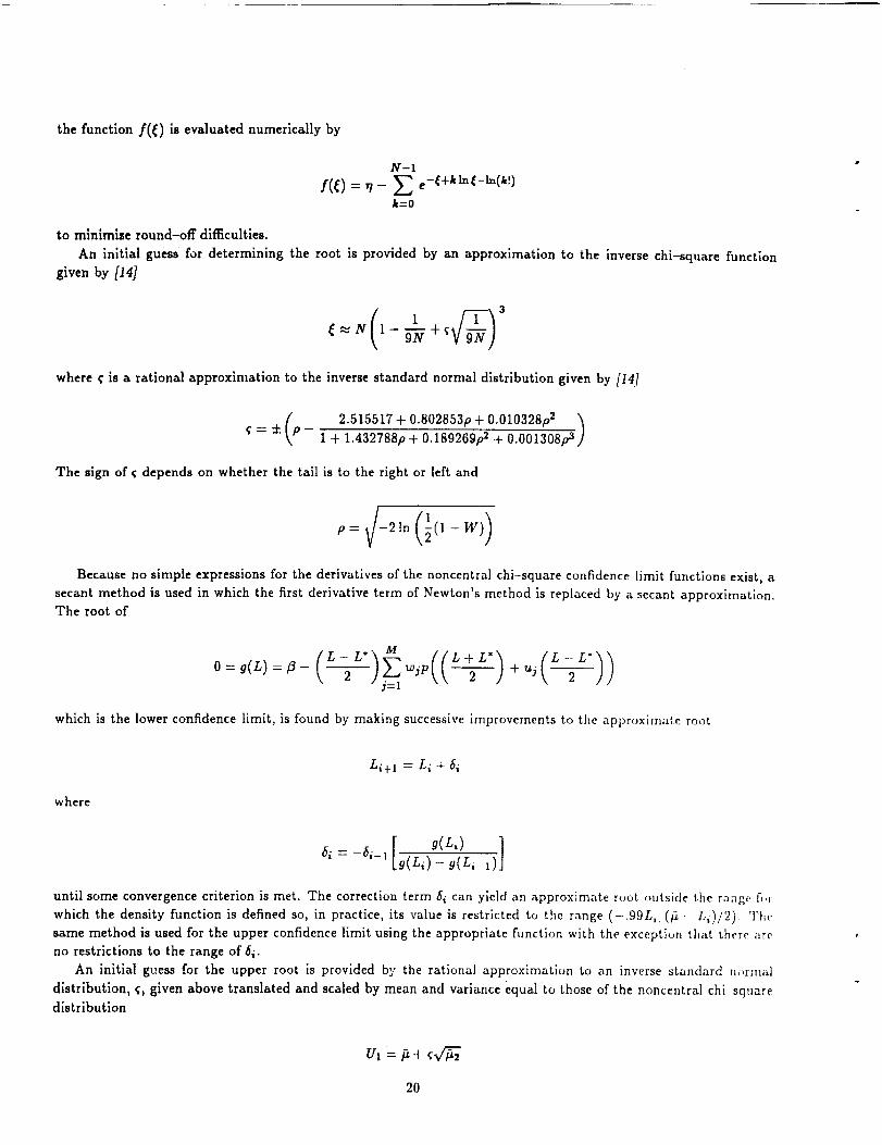
the function f(_) is evaluated numerically by

N-1

---k=O

to minimize round-off difficulties.

An initial guess for determining the root is provided by an approximation to the inverse chi-square function

given by [14]

3

_Iv i- _-_ + _

where q is a rational approximation to the inverse standard normal distribution given by [14]

q=+(p_ 2"515517 + 0"802853p + 0"010328p2 )l + l.432788p + O.189269prt + O.OO1308p3

The sign of c; depends on whether the tail is to the right or left and

Because no simple expressions for the derivatives of the noncentral chi-square confidence limit functions exist, a

secant method is used in which the first derivative term of Newton's method is replaced by a secant approximation.The root of

j=l

which is the lower confidence limit, is found by making successive improvements to the approximate root

Li+l = Li + 6i

where

6,=-6,_, [ L') ]- y(L,_I)

until some convergence criterion is met. The correction term 5i can yield an approximate root outside tile range fi)_

which the density function is defined so, in practice, its value is restricted to the range (-.99Li. (_ - Li)/2). The

same method is used for the upper confidence limit using the appropriate function with the exception that there _lre

no restrictions to the range of 6 i.

An initial guess for the upper root is provided by the rational approximation to an inverse standard m-,rmal

distribution, ¢, given above translated and scaled by mean and variance equal to those of the noncentral chi squaredistribution

UI = _ ÷ qv"_-

20

An initial guess for the lower root is provided in nearly the same way when R is large, except that the value is notallowed to be too small

/'1 ----max(_/10,/_-I- c;V_)

The approximation to the inverse chi-square function, given above, is used when R is less than 1/10. The first

increment to the initial guess of the root_ 61, is arbitrarily set to/:_2/10.

21

Appendix C: FORTRAN Program

The FORTRAN program CHISQR calculates theoretical confidence limits for a chi-square distribution and a

noncentral chi-square distribution. An example of program output is appended.

22

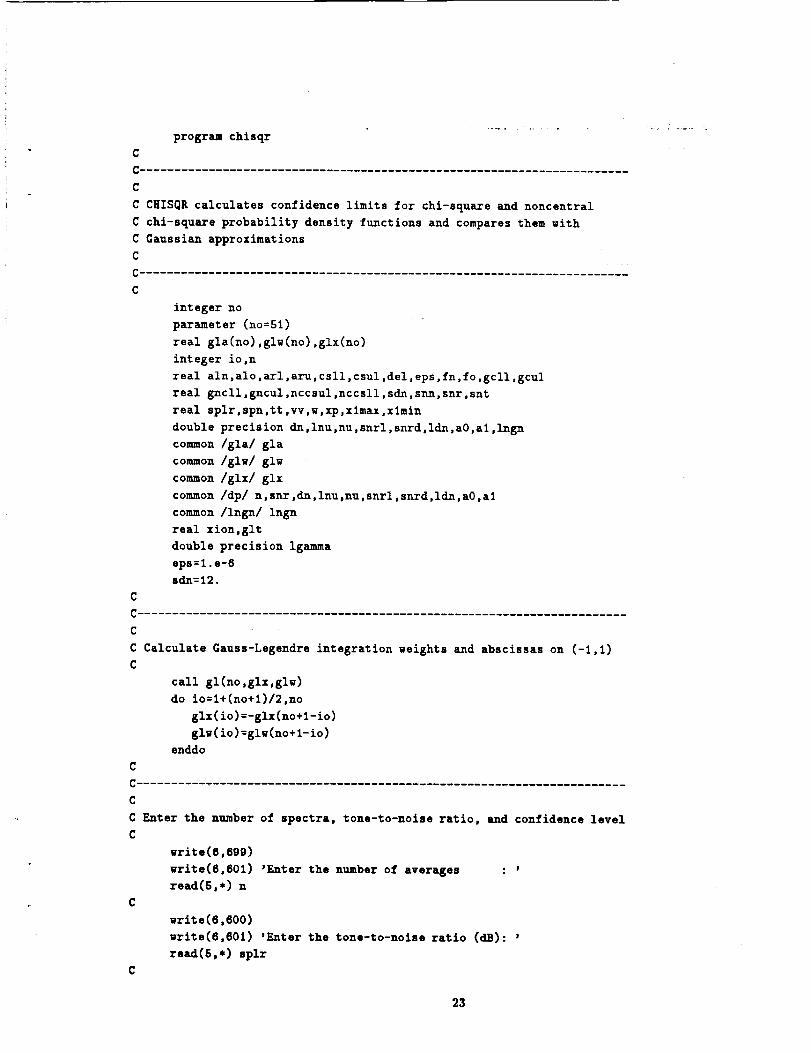
program chisqr

C

C CHISOR calculates confidence limits for chi-square and noncentral

C chi-square probability density functions and compares them with

C Gaussian approximations

C

C .......................

C

integer no

parameter (no=S1)

real gla(no),glw(no),glx(no)

integer io,n

real aln,alo,arl,aru,csll,csul,del,eps,fn,fo,gcll,gcul

real gncll,gncul,nccsul,nccsll,sdn,snn,snr,snt

real splr,spn,tt,vv,w,xp,xlmax,xlmin

double precision dn,lnu,nu,snrl,snrd,ldn,aO,a1,1ngn

common /gla/ gla

common /glw/ glw

common /glx/ glx

common /dp/ n,snr,dn,lnu,nu,snrl,snrd,ldn,aO0al

common /Ingn/ ingn

real xion,glt

double precision Igamma

eps=l .e-6

sdn=12.

C

C .......................

C

C Calculate Gauss-Legendre integration weights and abscissas on (-1,1)

C

call gl(no,glx,glw)

do io=1+(no+l)/2,no

glx(io)=-glx(no+l-io)

glw(io)=glw(no+1-io)

enddo

C

C ........

C

C Enter the number of spectra, tone-to-noise ratio, and confidence level

C

write(S,699)

write(6,601) 'Enter the number of averages ' '

read(5,*) n

write(6,600)

write(6,601) 'Enter the tone-to-noise ratio (dB): '

read(5,*) splr

23

write(6,600)

write(6,601) 'Enter the confidence level (_)

read(5,*) w

C

C ....................................

C

C First guess from standard normal distribution inverse

C

aru=.5*(1.+.Ol*w)

arl=.5*(1.-.Ol*w)

tt=sqrt(-2.*alog(arl))

xp=tt-(2.515517+tt*(.802853+tt*.O10328))

& /(1.+tt*(1.432788+tt*(.189269+tt*.O01308)))

C

C ........

: J

C

C Calculate tone and noise values

C

snr=lO.**(.l*splr)

snrd=lO.dO**(.ldO*splr)

spn=l.+snr

C

C Standard deviations of normal distributions

C

snn=l./sqrt(float(n))

snt=sqrt((1.+2.*snr)/n)

C

C Calculate preliminary values for EDSPDF

C

dn=dble(n)

ldn=dlog(dn)aO=dn*(ldn-snrd)

nu=dn-l.dO

if (n.gt.l) lnu=dlog(nu)

snrl=dlog(snrd)

al=2.dO*Idn+snrl

Ingu=Igamma(n)

C

C Confidence limits for noise by chi-square distribution

C

csul=lO.*alog10(xion(arl,n))

csll=10.*aloglO(xion(aru,n))

C

C Confidence limits by Gausslan approximation

C

gncll=lO.*aloglO(amaxl(1.258925412e-lO,(1.-xp.snt/spn)))

gncul=lO.*aloglO(1.+xp*snt/spn)

gcll=10.*alog10(amaxl(1.25892S412e-lO,(1.-xp,snn)))

gcul=lO.*aloglO(1.+xp*snn)

C

C ..............

24

C

C Integration limits

C

xlmax=spn+sdn*snt

xlmin=amaxl(0.,spn-sdn*snt)

C

C ...................................

C

C

C

C

C

C ..........

Search for confidence limits of noncentral chi-square using a

modified secant method for the lower limit and a secant method

for the upper limit

First guess at lower limit

aln=amax1(.1_spn,spn-xp_snt)

First guess if chi-square

if (splr.le.-10.) then

vv=l./(9.*n)

aln=amaxl(O.,((1.-vv-xp*sqrt(vv))**3))

endif

C

C .........

C

C First function evaluation

C

fn=glt(xlmin,aln)-arl

del=(spn-aln)*.06

C

C .........

C

C Repeat until there is an answer

C

1 continue

alo=aln

aln=alo+del

C

C Next function evaluation

C

fo=fn

fn=glt(xlmin,aln)-arl

C

C Next delta

C

if (fo.eq.fn) goto 2

del=amax1(-.99*aln,amin1(.6*(spn-aln),del*fn/(fo-fn)))

if (abs(del).lt.aln*epe) goto 2

25

goto 1C

C Convergence

C

2 continue

nccsll=lO.*aloglO(aln/spn)

C

C ...................................

C

C First guess at upper limit

C

C

C

C

aln=spn+xp*snt

C First function evaluation

C

fn=glt(xlmin,aln)-aru

del=snt*.1

C

C .........

C

C Repeat until there is an answer

C

3 continue

alo=aln

aln=alo+del

C

C Next function evaluation

C

fo=fn

fn=glt(xlmin,aln)-aru

C

C Next delta

C

if (fo.eq.fn) goto 4

del=de!*fn/(fo-fn)

if (abs(del).it.aln*eps) goto 4

goto 3C

C Convergence

C

4 continue

nccsul=lO.*aloglO(aln/spn)

C

C

C

C Write results

C

write(6,602) 'Noise'

write(8,600)

26

erite(6,603)

write(6,603)

write(6,604)

write(6,604)

write(6,602)

write(6,600)

write(6,603)

write(6,603)

write(6,604)

write(6,604)

write(6,699)

stop ' '

' Chi-Square ,,, Gaussian

J

'Upper llmit',csul,' dB',Ecul ,, dB'

'Lower limit' cs11,' dB',Ec11 ,, d3'

'Tone + Noise, ',splr,' dB T/N Ratio'

'Noncentral Chi-Square ,,, Gaussian

'Upper Limit',nccsul,' dB',gncul,' dB'

'Lower Limit',nccsll,' dB,,Encll ,, dB'

C

C Formats

600 format(x)

601 format(x,a,$)

602 format(////,x,a,2x,f6.1,a)

603 format(16x,a,a)

604 format(x,a,3x,(Sx,f9.4,a,Sx),(Sx,f9.4,a))

699 format(/)

end

L

27

real function edspdf(z)

CC Noncentralchi-squared probability density function of order 2nC

C

real z

integer n

real snr

double precision dn,lnu,nu,snrl,snrd,ldn,aO0al,lnE n

common /dp/ n,snr,dn,lnu,nu,snrl,snrd,ldn,aO,al

common /lngn/ lngn

integer k

real qeta,qim,qin,qio,qip,qrho,qt,qti,qt2,qx,qzeta

double precision eps

double precision zz,zO

double precision bO,bl

double precision lnxi,lnxim,pdf,xi,lncf

double precision s

double precision zn,zs,eta,us,den,z2

double precision t,tt,ttt,tttt,ttttt

eps=l.d-16

C

C Evaluate PDF using polynomial approximation when N=I

C (Abramowitz and Stegunp 378)C

k

k

k

k

if (n.eq.1) then

if (z.eq.O.) then

edspdf=exp(-snr)

else

qeta=sqrt(snr)

qzeta=sqrt(z)

qx=2.*qeta*qzeta

qt=qx/3.75

if (qt.lt.1.) then

qt2=qt*qt

qio=l.

+qt2.(3.5156229

+qt2.(3.0899424

+qt2.(1.2067492

+qt2.(0.2659732

+qt2.(0.0360768

+qt2.(0.0045813))))))

edspdf=qio*exp(-(snr+z))

else

28

qti=l./qt

qim=0.39894228

+qti*(0.01328592

& +qti*(0.00225319

+qti*(-.00157585

• +qti*(0.00918281

• +qti*(-.02087706

• +qti*(0.02635537

• +qti*(-.01647633

• +qti*(O.OO392377))))))))

qrho=qzeta-qeta

edspdf=qim*exp(-qrho*qrho)/sqrt(qx)endif

endif

return

endif

C

C Evaluate PDF using polynomial approximation when N=2

C (Abramowitz and Stegunp 378)

if (n.eq.2) then

if (z.eq.O.) then

edspdf=O.

else

qeta=sqrt(snr)

qzeta=sqrt(z)

qx=4.*qeta*qzeta

qt=qx/3.75

if (qt.lt.1.) then

qt2=qt*qt

qip=0.5

• +qt2.(0.87890594

• +qt2*(O.S1498869

• +qt2.(0.15084934

• +qt2.(0.02658733

• +qt2.(0.00301632

• *qt2.(0.00032411))))))

edspdf=8.*z*qlp*exp(-2.*(snr+z))

else

qti=l./qt

qtn=0.39894228

• +qti*(-.03988024

• +qti*(-.00362018

• +qti*(0.00163801

• +qti*(-.01031885

• +qti*(0.02282967

• +qti*(-.02898312

& +qti*(0.01787684

29

& +qti*(-.00420059))))))))

qrho=qzeta-qeta

edspdf=sqrt(qzeta/(snr*qeta))*qin*exp(-2_,qrho,qrho)endif

endif

return

endif

C

C Evaluate PDF when N>2

C

if (z.eq.O.) then

if (n.gt.1) then

edspdf=O.

else

edspdf=exp(-snr)

endif

return

endif

zz=dble(z)

if (snrd.gt.l.d-5) then

if (dn+dloglO(s_rd).gt.3.dO) thenC

C Uniform asymptotic approximation (Abramowitz and Stegun p 378)C

zn=2.dO*(n/nu)*dsqrt(snrd*zz)

z2=zn*zn

if (zn.gt.2.dO) then

zs=zn*dsqrt(1.dO+l.dO/z2)

else

zs=dmaxl(1.dO,dsqrt(1.dO+z2))

endif

t=l.dO/zs

tt=t*t

ttt=t*tt

tttt=tt*tt

ttttt=tt*ttt

if (zn.gt.2.dO) then

eta=zs+dlog(l.dO/(l.dO/zn+dsqrt(l.dO+l.dO/z2)))

else

eta=zs+dlog(zn/(l.dO+dsqrt(l.dO+z2)))

endif

us=l.dO

den=nu

us=us+t*(.125dO

i +tt$(-.2083333333333333dO))/den

den=den*nu

us=us+tt*(.OTO3125dO

k +tt*(-.4010416666666667dO

+tt*(.3342013888888889dO)))/den

3O

den=den*nu

us=us+ttt*(.O73242187SdO

• +tt*(-.8912109375dO

• +tt*(1.846462673611111dO

• +tt*(-1.O25812S96450617dO))))/denden=den*nu

us=us+tttt*(.l1215209960937SdO

• +tt*(-2.3640869140625dO

• +tt*(8.78912353515625dO

• +tt*(-11.20700261622299dO

• +tt*(4.669584423426248dO)))))/den

den=den*nu

us=us+ttttt*(.2271080017089844dO

• +tt*(-7.368794359479632dO

• +tt*(42.53499874638846dO

• +tt*(-91.81824154324002dO

• +tt*(84.63621767460074dO

• +tt*(-28.21207255820025dO))))))/den

den=den*nu

us=us+ttt*ttt*(.S72SO14209747314dO

• +tt*(-26.49143048695155dO

• +tt*(218.1905117442116dO

• +tt*(-699.S796273761326dO

• +tt*(1059.990452528dO

• +tt*(-765.2S24681411817dO

• +tt*(212.STO1300392171dO)))))))/den

xl=dn*((nu/dn)*eta-(zz+snrd))

xi=xi+Idn-.SdO*dlog(zs)-.SdO,Inu

xl=xi+.SdO*nu*(dlog(zz)-snrl)

xi=xi-O.918938533204673dO

xi=xi+dlog(us)

edspdf=sngl(dexp(xi))

else

C

C Ascending series (Abramowitz and Stegunp 375)C

zO=dlog(zz)

bO=aO+nu*zO-dn*zz

bl=al+zO

pdf=O .dO

k=O

incf=lngn

Inxim=bO-Incf

1 continue

lnxi=bO+bl*k-lncf

if ((lnxt.lt.lnxim).and.(pdf.eq.O.dO)) goto 3

if (lnxt.lt.-3OO.dO) goto 2

xi=dexp(lnxi)

pdf=pdf+xi

if (xt.le.eps*pdf) goto 32 continue

31

k=k+l

Incl=Incf+dlog(dble(k))+dlog(dbls(n+k-1))

goto 1

3 continue

edspdf=sngl(pdf)

endif

else

C

C Broadband approximation _hen tone-to-broadband ratio is smallC

if (n.eq.1) then

edspdf=sngl(dn*dexp(-zz))else

if (z.eq.O.) then

edspdf=O.

else

s=zz_dn

edspdf=sngl(dexp(ldn+nu*dlog(s)-(s+lngn)))endif

endif

endif

return

end

32

doubleprecision function Igamma(n)

C

C Natural logaritDu, of the gamma function, G(n)

C

C ...........

C

C

C

integer n

integer i

double precision nn,in,ins

C

C Evaluate gamma function (Abramowitz and Stegun p 2S7)

C

if (n.lt.lO0) then

Igamma=O.

if (n.gt.2) then

do i=3,n

igamma=Igamma+dlog(i-l.dO)

enddo

endif

else

nn=dble(n)

in=l.dO/nn

ins=in*in

Igamma=(nn-.SdO)*dlog(nn)-nn

Igamma=Igamma+O.918938533204673dO

Igamma=Igamma+in*(+8.333333333333333d-2

+ins*(-2.777777777777778d-3

& +ins*(+7.936507936607937d-4

& +ins*(-5.9523809523809S2d-4))))

endif

return

end

_L

33

C

C

real function xion(a,n)

C

C

C

C Solve :

C

C

C

k

-x N-1 x

A -- e SUM ---

k--O k!

for x Eiven A and _, return x/N.

C

real a

integer n

double precision delt,eps,fxio,xin,xio,lfnk,d,xiol

real vv,t,xp

inteEer k

C

C Modified second order gegton's method _hen N>I (Davis and Rabinowitz

C p 114) (first estimate by Abramowitz and Stegun p 941 via p 933)C

xin=-dlog(dble(a))

if (n.gt.1) then

vv=l./(9.*n)

if (a.lt.O.5) then

t=sqrt(-2.*dlog(dble(a)))

xp=t-(2.515517+t*(.802853+t_.010328))

& /(1.+t*(1.432788+t*(.189269+t_.O01308)))

xin=n*(1.-vv+xp_sqrt(vv))_3

else

t=sqrt(-2._dlog(l.dO-a))

xp=t-(2.SiSSlT+t_(.802853+t*.O10328))

/(1.+t*(l.432788+t*(.189269+t*.O01308)))

xin=n_(1.-vv-xp*sqrt(vv))_,3

endif

eps=1.d-8

continue

xio=xin

xiol=dlog(xio)

fxio=dexp(-xio)

Ifnk=O.dO

do k=l,n-1

Ifnk=Ifnk+dlog(dble(k))

fxio=fxlo+dexp(k*xiol-lfnY-xlo)

enddo

delt=(fxio-a)*dexp(xio+lfnk+(1-n),xiol)

d=dmaxl(.IdO,dminl(2.dO,l.dO-delt,(.SdO,((n-i)/xio-l.dO))))

xin=xio+d_delt

34

C

if (dabs(d*delt).gt.dabs(xio*eps)) goto 1

endif

xion=sngl(xin/n)

return

end

35

real function glt (_aain,xmax)

C

C ....... -- .............

C

C Adjust Gauss-Legendre abcissas and integrate the PDF

C

C

C

C

integer no

parameter (no=51)

real gla(no),glw(no),glx(no)

common /gla/ gla

common Iglwl glw

common /glx/ glx

real xmin,xmax

integer io

real hr,ta

real edspdf

C

C Adjust Gauss-Legendre abcissas for interval (xmin,xmax)

C

hr=.5*(xmax-xmin)

t a=xmax+xmin

do io=1,(no+1)/2

gla(io)=xm±n+hr*(1.+glx(io))

enddo

do io=l+(no+l)/2,no

gla(io)=ta-gla(no+l-io)

enddo

C

C Integrate the PDF over (xmin,xmax)

C

glt=O.

do io=l,no

glt=glt+glw(io)*edspdf(gla(io))

enddo

glt=hr*glt

return

end

36

subroutinegl(n,x,w)

C

C Calculate Gauss-Legendre integration abscissas and weights on (-1,1)C

C

real x(1),e(1)

integer i,k,m,n

real den,dp,dpn,dl,d2pn,d3pn,d4pn,el

real fx,h,p,pk,pkml,pkpl,t,tl,u,v,xO

C

C Find Gauss-Legendre integration abscissas and weights on (-1,1)

C (Davis and Rabinowitz p 487)

C

m=(n+l)/2

e1=n* (n+ 1)do i=1,m

t= (4"i-1) *3. 1415926536/(4,n+2)

xO=(1.-(1.-1./n)/(8.,n,n,_),cos(t)

pkml=l.

pk=xO

do k=2,n

t l=xO*pk

pkp 1= t1-pkm 1- (t 1-pkm I)/k+t 1

pkm l=pk

pk =pkp 1

enddo

den= 1. -xO*xO

dl=n* (pkml-xO*pk)

dpn=dl/den

d2pn= (2. *xO*dpn-e l*pk)/den

d3pn= (4. *xO *d2pn+ (2. - •1 )*dpn )/den

d4pn= (6. *xO*d3pn+ (6. -el )*d2pn)/den

u=pk/dpn

v=d2pn/dpn

h=-u* (1. +. 5*u* (v+u* (v*v-d3pn/(3. *dpn) ) ) )

p=pk+h* (dpn+. 5*h* (d2pn+h/3. * (d3pn+. 25*h*d4pn) ) )

dp=dpn+h* (d2pn+. 5*h* (d3pn+h*d4pn/3.) )

h=h-p/dp

•(i)=xO+h

fx=dl-h*e 1" (pk+. 5*h* (dpn+h/3. * (d2pn+. 25.h* (d3pn+. 2*h*d4pn) )))

,(i)=2.*(1 .-xCi)*xCi))/Cfx*fx)

enddo

if (m+m.gt.n) x(m)=O.

return

end

37

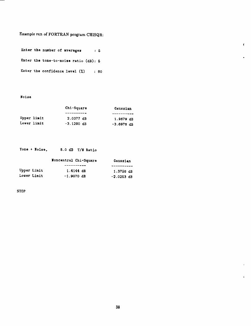
Example run of FORTRAN program CHISQR:

Enter the number of averages : 5

Enter the tone-to-noise ratio (d3): 5

Enter the confidence level (_) : 80

Noise

Chi-Square Gaussian

Upper limit 2.0377 dB 1.9679 dB

Lower limit -3.1290 dB -3.6978 dB

Tone + Noise,

Upper Limit

Lower Limit

STOP

8.0 dB T/N Ratio

Noncentral Chi-Square

1.4144 dB

-1.9070 dB

Gaussian

1.3758 dB

-2.0253 dB

38

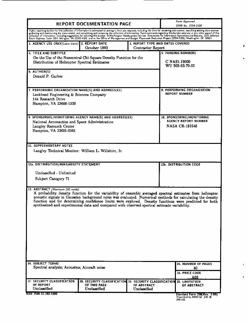
Form Appro red

REPORT DOCUMENTATION PAGE OMB No. 0704-0188

Public reporting burden for this collection of information is estimated to average I hour per response, including the time for reviewing instructions_ searching existing data sources.

gathering and maintalnin_ the data needed, and completing and reviewing the collection of information Send comments regarding this burden estimate or any other aspect of this

collection of information, including suggestions for reducing this burdem toWashington Headquarters Services, Directorate for Information Operations and Reports_ 1215 Jefferson

Davis Highway Suite 1204=Arlington,VA 22202 4302, and to the Officeof Managementand Budget,PaperworkReductionProject(0704-0188), Washington DC 20503.

1. AGENCY USE ONLY(Leave b/ank) 2. REPORT DATE 3. REPORT TYPE AND DATES COVERED

October 1993 Contractor Report4. TITLE AND SUBTITLE

On the Use of the Noneentral Chi-Square Density Function for theDistribution of Helicopter Spectral Estimates

6. AUTHOR(S)Donald P. Garber

7. PERFORMING ORGANIZATION NAME(S) AND ADDRESS(ES)

Lockheed Engineering & Sciences Company

144 Research Drive

Hampton, VA 23666-1339

9. SPONSORING/MONITORING AGENCY NAME(S) AND ADDRESS(ES)

National Aeronautics and Space AdministrationLangley Research CenterHampton, VA 23681-0001

5. FUNDING NUMBERS

C NASI-19000WU 505-63-70-02

8. PERFORMING ORGANIZATION

REPORT NUMBER

10. SPONSORING/MONITORINGAGENCY REPORT NUMBER

NASA CR-191546

Ill. SUPPLEMENTARY NOTES

Langley Technical Monitor: William L. Willshire, Jr.

12a. DISTRIBUTION/AVAILABILITY STATEMENT 12b. DISTRIBUTION CODE

Unclassified - Unlimited

Subject Category 71

13. ABSTRACT (Maximum 200 words)

A probability density function for the variability of ensemble averaged spectral estimates from helicopteracoustic signals in Gaussian background noise was evaluated. Numerical methods for calculating the densityfunction and for determining confidence limits were explored. Density functions were predicted for bothsynthesized and experimental data and compared with observed spectral estimate variability.

II I

14. SUBJECT TERMS

Spectralanalysis;Acoustics;Aircraftnoise

I

17. SECURITY CLASSIFICATIONOF REPORT

Unclassified

JSN 1540-0]-280-5500

18. SECURITY CLASSIFICATIOI_

OF THIS PAGE

Unclassified

19. SECURITY CLASSIFICATION

OF ABSTRACT

Unclassified

15. NUMBER OF PAGES

4016. PRICE CODE

A0320. LIMITATION

OF ABSTRACT

I II

Standard Form 29B(Rev. 2-B9)Prescribedby ANSI Std. Z39-t8298-102