Optimal Control of a Production-Inventory System with

both Backorders and Lost Sales†

Saif Benjaafar1 • Mohsen ElHafsi2 • Tingliang Huang3

1Industrial & Systems Engineering, Department of Mechanical Engineering,

University of Minnesota, Minneapolis, MN 55455, saif@umn.edu

2The A. Gary Anderson Graduate School of Management, University of California, Riverside, CA 92521-0203, mohsen.elhafsi@ucr.edu

3Kellogg School of Management, Northwestern University, Evanston, IL 60208,

tingliang-huang@kellogg.northwestern.edu

December 6, 2007

Abstract

We consider the optimal control of a production inventory-system with a single product and two customer classes where items are produced one unit at a time. Upon arrival, customer orders can be fulfilled from existing inventory, if there is any, backordered, or rejected. The two classes are differentiated by their backorder and lost sales costs. At each decision epoch, we must determine whether or not to produce an item and if so, whether to use this item to increase inventory or to reduce backlog. At each decision epoch, we must also determine whether or not to satisfy demand from a particular class (should one arise), backorder it, or reject it. In doing so, we must balance inventory holding costs against the costs of backordering and lost sales. We formulate the problem as a Markov decision process and use it to characterize the structure of the optimal policy. We show that the optimal policy can be described by three state-dependent thresholds: a production base-stock level and two order-admission levels, one for each class. The production base-stock level determines when production takes place and how to allocate items that are produced. This base-stock level also determines when orders from the class with the lower shortage costs (class 2) are backordered and not fulfilled from inventory. The order-admission levels determine when orders should be rejected. We show that the threshold levels are monotonic (either non-increasing or non-decreasing) in the backorder level of class 2. Using numerical results, we compare the performance of the optimal policy against several heuristics and show that those that do not allow for the possibility of both backordering and rejecting orders can perform poorly. Key words: Production and inventory control, make-to-stock queues, inventory rationing, admission control, Markov decision processes

† Authors are listed alphabetically

1. Introduction

Inventory problems treated in the literature fall mostly into two categories. One deals with systems

where backordering is always allowed. The other deals with systems where backorders are not allowed

and orders are considered lost if not fulfilled immediately. In practice, it is however common to have

systems where both features, backorders and lost sales, are present. Backorders are allowed if the number

of orders already backlogged is not too high but orders are rejected, or fulfilled through other means,

otherwise. Systems with both features are obviously superior to ones that allow one but not the other.

Such systems are also consistent with human behavior since customers are generally willing to wait but

are not infinitely patient. Unfortunately, the analysis of systems with both backordering and lost sales is

notoriously difficult. In fact, very little is known about optimal control policies or even effective

heuristics for such systems. More significantly, little is known about the value of permitting both

backorders and lost sales.

In this paper we address some of these limitations in the context of a production-inventory system

with two classes of customers. In particular, we consider a continuous time and continuous review system

where demand orders from each class arrive continuously over time one unit at a time with stochastic

inter-arrival times. With each order arrival, a decision must be made on whether to fulfill the order from

on-hand inventory, backorder it, or reject it. There are costs associated with the backordering and

rejecting of orders, which can vary from class to class. Inventory is replenished from a production facility

that produces units one at time with stochastic production times. At any point in time, the system manager

must decide on whether or not to produce and whether a produced item should be allocated to increase

on-hand inventory or reduce backorders from one of the two classes, if there are any.

We formulate the problem as a Markov decision process (MDP) and characterize the structure of the

optimal policy. We show that the optimal policy can be described by three state-dependent thresholds: a

production base-stock level and two order-admission levels, one for each class. The production base-

stock level determines when production takes place and how to allocate items that are produced. This

base-stock level also serves as an inventory rationing threshold and determines when orders from the

class with the lower shortage cost (class 2) are backordered and not fulfilled from inventory. The order-

admission levels determine when orders from each class are rejected. We show that all three threshold

levels are monotonic (either non-increasing or non-decreasing) in the backorder level of class 2.

1

Our results generalize several known results for simpler problems, such as those involving systems

with only backorders or only lost sales. Our results can also be specialized to admission control problems

in systems where inventory cannot be held (so-called make-to-order systems), leading to new results for

that class of problems. Using numerical results, we compare the performance of the optimal policy

against several heuristics and show that those that do not allow for the possibility of both backordering

and rejecting or those that do not differentiate between customer classes can perform poorly. On the other

hand, we find that a heuristic policy that mimics the optimal policy but uses fixed thresholds, instead of

ones that are state-dependent, performs well over a wide range of parameters.

Our paper is most closely related (in its theme) to the literature on inventory systems with partial

backordering. A common assumption in that literature is that an arriving customer that faces a stockout is

backordered with a certain probability and is lost otherwise (see for example Montgomery et al. 1981,

Moinzadeh 1989, Smeitink 1990, Nahmias and Smith 1994, and the references therein). In situations

where multiple orders are placed at once, this means that a fraction of customers are backordered while

the remainder is lost. These probabilities or fractions are assumed to be exogenous and are supposed to

reflect the willingness of customers to wait. Some authors have used a patience threshold to model

customer’s willingness to wait. For example, Posner (1981) and Das (1977) assume that customers are

initially willing to wait, but if their demand is not fulfilled within their patience threshold time, they leave

the system. In all of these papers, partial backordering is an outcome of customer behavior and not a

decision variable. A notable exception is Rabinowitz et al. (1995) who assume that backorders are

allowed but cannot exceed a certain fixed threshold. With no exception, all the above papers, assume a

particular form for the inventory control policy, typically a base-stock or a (q, r) policy.

In addition to the literature on partial backordering, our paper is related to the literature on inventory

systems with multiple customer classes. Examples from this literature include Topkis (1968), Nahmias

and Demmy (1981), Cohen et al. (1988), Frank et al. (2003), Deshpande et al. (2003) and the references

therein. Papers that consider production-inventory systems, in the same way we do in this paper, include

Ha (1997a, 1997b), de Véricourt et al. (2002), and Carr and Duenyas (2003). In each case, the authors

show that there exists a threshold associated with each customer class such that it is optimal to fulfill

demand from that class if on-hand inventory is above this threshold. Otherwise, depending on the

assumption, demand from that class is backordered or lost. Most of this literature assumes either complete

2

backordering or complete lost sales. There does not appear to be any papers that consider both backorders

and lost sales when there are multiple customer classes.

Finally, our paper is more broadly related to the literature on admission control in queueing systems.

A queueing system can be viewed as the make-to-order counter-part to the make-to-stock system we

consider in this paper. Reviews of this literature can be found in Stidham (1985), Altman (2001) and

Koole (2007). In Section 4.2, we show how results we obtain in this paper can be applied to admission

control problems to obtain new results regarding the structure of optimal policies in those settings.

Relative to the existing literature, our paper makes the following contributions. It appears to be the

first to characterize the structure of the optimal policy in systems where both backorders and lost sales are

allowed and appears to be the first to do so in the context of systems with two customer classes. The

results we present generalize several known results for simpler systems and apply to several other related

problems, including admission control problems. Moreover, our paper offers what appears to be the first

evidence regarding the performance of several heuristics against the optimal policy and to assess the

benefit of policies that permit both backordering and lost sales.

The rest of the paper is organized as follows. In Section 2, we formulate the problem. In Section 3, we

characterize the structure of the optimal policy. In Section 4, we discuss various special cases and related

problems. In Section 5, we present results from a numerical study that evaluates the performance of the

optimal policy against heuristics. In Section 6, we offer a summary and some concluding comments. 2. Problem Formulation

We consider a system where a single product is produced at a single facility to fulfill demand from two

customer classes. Items are produced one unit at a time with exponentially-distributed production times

with mean 1/μ. The production facility can produce ahead of demand in a make-to-stock fashion.

However, items in inventory incur a holding cost h per unit per unit time. Customers place orders

continuously over time according to a Poisson process with rate λi for customer class i, i = 1; 2. Upon

arrival, an order is either fulfilled from inventory, if any is available, backordered, or rejected. Orders

from class i that are backordered incur a backordering cost bi per unit per unit time, while orders that are

rejected incur a lost sale cost ci per unit, for i = 1, 2. We assume that penalties for shortage are higher for

class 1, so that b1 ≥ b2 and c1 ≥ c2. This assumption is consistent with settings where one customer class is

3

less tolerant of shortages (either delays or rejection) and, consequently, imposes higher penalties when

they occur.

At any point in time, the system manager must decide whether or not to produce an item. If a unit is

produced, a decision must also be made on whether to use it to increase inventory or to reduce backlog

from one of the two classes, if there is any. We assume that preemption is possible, so that deciding not to

produce could mean interrupting the production of a unit that was previously initiated. If interruption

occurs, we assume it can be resumed the next time production is initiated (because of the memoryless

property of the exponential distribution, resuming production from where it was interrupted is equivalent

to initiating it from scratch). We assume that there are no costs associated with interrupting production.

This conforms to earlier treatment of production-inventory systems in the literature; see, for example, Ha

(1997a, 1997b). This assumption is not restrictive since, as we show in Theorem 1, it turns out that it is

never optimal to interrupt production of an item once it has been initiated.

At any point in time, the system manager must also decide on how to handle incoming orders. Should

an order from class i arise, a decision must be made on whether to fulfill it from on-hand inventory, if

there is any, to backorder it, or to reject it. For orders from class 1, it is obvious that, if there is on-hand

inventory, orders should be fulfilled immediately (we provide a rigorous proof for this in Section 3).

However, for orders from class 2, it may be advantageous to reserve on-hand inventory for future orders

from class 1, given the higher shortage penalties for class 1. If an order, regardless of its class, is not

fulfilled from inventory, then a decision must be made on whether it should be backordered or rejected. It

may be more desirable to reject an order rather than backorder it if there is already a large backlog of

orders from either class.

In our model, we assume that demand is Poisson and both production times and times between

consecutive updates are exponentially distributed. These assumptions are made in part for mathematical

tractability as they allow us to formulate the control problem as an MDP and enable us to describe the

structure of an optimal policy. They are also useful in approximating the behavior of systems where

variability is high. The assumptions of Poisson demand and exponential production times are consistent

with previous treatments of production-inventory systems; see for example, Buzacott and Shanthikumar

(1993), Ha (1997a, 1997b), Zipkin (2000), and de Véricourt et al. (2002) among others. In Section 5, we

discuss how these assumptions may be partially relaxed.

4

The state of the system at time t can be described by the pair ( ( ), ( ))X t Y t , where

( ) max(0, ( ))X t + = X t denotes on-hand inventory, ( ) max(0, ( ))X t − X t= − denotes backorder level for

customer class 1, and Y(t) denotes backorder level for customer class 2. Note that because of the

possibility of interrupting production, it is not necessary to include in the state description whether an

item is currently being produced or not. Furthermore, because both order inter-arrival times and

production times are exponentially distributed, the system is memoryless and decision epochs can be

restricted to only times when the state changes (i.e., the completion of an item or the fulfillment of an

order). The memoryless property allows us to formulate the problem as an MDP and to restrict our

attention to the class of Markovian policies for which actions taken at a particular decision epoch depend

only on the current state of the system.

In each state, the system manager makes two types of decisions, one regarding production and the

other regarding order fulfillment. For production, the choice is between not producing, producing to

increase net inventory (either to increase on-hand inventory or decrease backorder level for class 1), and

producing to reduce backorder level from class 2. For order fulfillment, the choice is between fulfilling an

order, should one arise, from on-hand inventory, backordering the order, or rejecting it. A policy π

specifies for each state x = (x, y), the action 0 1 2( , ) ( , , )a x y u u uπ = , where 0 0u = means do not produce,

means produce to increase net inventory, 0 1u = 0 2u = means produce to reduce backorders from class 2,

means reject demand from class 1, 1 0u = 1 1u = means accept demand from class 1 (either satisfy it from

on-hand inventory if x > 0 or backorder it otherwise), 2 0u = means reject demand from class 2, 2 1u =

means satisfy demand from class 2 from on-hand inventory, and 2 2u = means backorder demand from

class 2. For example, the action a = (2,1,0) specifies that whenever the system is in state (x, y), we

should produce to reduce backorder level for class 2, accept orders from class 1, and reject orders from

class 2.

( , )x yπ

Let Ni(t) denote the number of orders from class i that have been rejected up to time t. Then the

expected discounted cost (the sum of inventory holding, backorder, and lost sales costs) over an infinite

planning horizon obtained under a policy π and a starting state (x, y), can be written as: ( )vπ x

( ) 2( , ) 1 2 10 0

( , ) [ ( ) ( ) ( ) ( )],t tx y i ii

v x y E e hX t b X t b Y t dt e c dN tπ π α α∞ ∞− + − −=

= + + + ∑∫ ∫ (1)

where α > 0. (Extending the analysis to the case where the objective is to minimize average cost is

straightforward and is briefly described at the end of Section 3). Our objective is to choose a policy *π

that minimizes the expected discounted cost. We refer to the optimal cost function as where *,v ** .v vπ≡

5

Following Lippman (1975), we work with a uniformized version of the problem in which the

transition rate in each state under any action is 1 2β μ λ λ= + + so that the transition times 0 = t0 ≤ t1 ≤ t2 ≤

… are such that the times between transitions {tj+1 – tj: j ≥ 0} form a sequence of i.i.d. exponential random

variables, each with mean 1/β. This leads to a Markov chain defined by {Zj: j ≥ 0} where

( ( ), ( ))j j jX t Y t=Z is the state resulting from the j-th transition. The introduction of the uniform transition

rate allows us to transform the continuous time decision process into a discrete time decision process,

simplifying the analysis considerably. To further simplify the analysis, and without loss of generality, we

also rescale time by letting α + β = 1. The optimal cost function can now be shown to satisfy the

following optimality equation:

*v

* * *

1 2 0 1 1 2 2( , ) ( , ) ( , ) ( , ),v x y hx b x b y T v x y T v x y T v x y*μ λ λ+ −= + + + + + (2)

where the operators Ti, i = 0, …, 2, are defined as follows:

{ }{ }0

min ( , ), ( 1, ), ( , 1) if 0( , )

min ( , ), ( 1, ) if 0,v x y v x y v x y y

T v x yv x y v x y y

⎧ + −⎪= ⎨>

+ =⎪⎩ (3)

{ }1 ( , ) min ( 1, ), ( , ) ,T v x y v x y v x y c= − + 1 (4)

and { }{ }

22

2

min ( 1, ), ( , 1), ( , ) if 0( , )

min ( , 1), ( , ) if 0.v x y v x y v x y c x

T v x yv x y v x y c x

⎧ − + +⎪= ⎨>

+ +⎪⎩ ≤

,

(5)

Operator T0 is associated with the decision of whether or not to produce. If y = 0 (there are no

backorders from class 2), then the choice is between not producing and producing to increase net

inventory from x to x+1. If y > 0, we must also consider the option of producing to reduce backorders for

class 2 from y to y -1. Operator T1 is associated with the decision of how to handle an order from class 1.

The choice is between rejecting the order and incurring the lost sale cost c1 or accepting the order (by

either fulfilling it from on-hand inventory, if there is any, or backordering it). Accepting the order reduces

net inventory from x to x-1. Similarly, operator T2 is associated with the decision of how to handle orders

from class 2. The choice here is between rejecting the order which leaves the state unchanged,

backordering it which increases backorder level from y to y+1, or fulfilling (if there is on-hand inventory)

which reduces net inventory from x to x-1. Note that in determining the optimal action at a state (x, y), the

optimal cost function is evaluated at each of the states to which the system would transition if any of

the feasible actions is taken. For production, this means comparing and

*v

* ( , ),v x y * ( 1, )v x y+ * ( , 1),v x y −

and choosing the action that corresponds to the lowest value. For order fulfillment for class 1, this means

6

comparing and while for orders from class 2 the comparison is between

and

*1( , )v x y c+ * ( 1, )v x y− ,

.*2( , ) ,v x y c+ * ( , 1),v x y + * ( 1, )v x y−

3. The Structure of the Optimal Policy

In this section, we characterize the structure of an optimal policy. In order to do so, we show that the

optimal value function for all states (x, y) satisfies certain properties as specified in Definition 1

below. We then show that these properties imply a specific rule for the optimal action in each state.

* ( , )v x y

Definition 1: Let V be the set of functions defined on +× such that if v∈V, then

A1: for x < 0 and y ≥ 0 and ( 1, ) ( , ) 0v x y v x y+ − ≤ ( 1, ) ( , 1) 0v x y v x y+ − − ≤ for x < 0 and y > 0;

A2: for all x and y>0; ( , 1) ( , ) 0v x y v x y− − ≤

A3: for all x and y; ( 2, ) ( 1, ) ( 1, ) ( , )v x y v x y v x y v x y+ − + ≥ + −

A4: for all x and all y; ( , 2) ( , 1) ( , 1) ( , )v x y v x y v x y v x y+ − + ≥ + −

A5: for all x and y; ( 1, 1) ( , 1) ( 1, ) ( ,v x y v x y v x y v x y+ + − + ≤ + − )

)A6: for all x and y > 0; ( 2, ) ( 1, 1) ( 1, ) ( , 1v x y v x y v x y v x y+ − + − ≥ + − −

A7: for all x and y > 0; and ( 1, 1) ( , ) ( 1, ) ( , 1)v x y v x y v x y v x y+ + − ≥ + − −

A8: for x > 0 and all y. 1( , ) ( 1, )v x y v x y c− − ≥ −

Lemma 1: If v∈V , then Tv ∈V , where * * *1 2 0 1 1 2 2( ) ( , ) ( , ) ( , ).Tv x hx b x b y T v x y T v x y T v x yμ λ λ+ −= + + + + +

Furthermore, the optimal cost function is an element of V. That is, ∈V. *v *v

A proof of Lemma 1 and of all subsequent results can be found in the Appendix. In the proof, we first

show that the operator T preserves properties A1-A8, which together with the convergence of value

iteration, allows us to conclude that the optimal cost function satisfies properties A1-A8. Applied to

property A1 indicates that, whenever there are backorders from class 1 (x < 0), it is preferable to

increase net inventory by one unit than to leave it unchanged. It is also preferable to increase net

inventory by one unit than to reduce backorders from class 2 by one unit (i.e., reducing backorders from

class 1 takes precedence over reducing backorders from class 2). Property A2 indicates that, for a fixed

level of net inventory, the fewer backorders from class 2 the better. Property A3 implies that the marginal

cost difference due to increasing net inventory (for a fixed level of backorders from class 2) is non-

increasing. Similarly, A4 implies that the marginal cost difference due to increasing backorders from class

2 (for a fixed level of net inventory) is non-increasing. In other words, A3 and A4 indicate that the

*v* ,v

7

optimal cost function is component-wise convex in x and y. Property A5 indicates that the marginal

cost difference due to increasing net inventory is non-increasing in the number of backorders from class

2. In other words, is submodular in the direction (x, y). Property A6 indicates that the cost difference

due to jointly increasing inventory and backorders by one unit each is non-decreasing in net inventory,

while A7 indicates that the cost difference due to jointly increasing inventory and backorders by one unit

each is non-decreasing in the backorder level. Property A8 implies that reducing on-hand inventory by

one unit is preferable to leaving it unchanged and incurring the lost sale cost c

*v

*v

1.

In order to describe the optimal policy implied by the above properties, we define the following three

threshold functions: { }{ }

* **

* *

min | ( 1, ) ( , 1) 0 if 0( )

min | ( 1, ) ( , ) 0 if 0,x v x y v x y y

s yx v x y v x y y

⎧ + − − > >= ⎨ + − >⎩ =

(6)

{ }* * *1 1( ) min | ( , ) ( 1, )w y x v x y v x y c= − − ≥ − , (7)

and { }{ }

{ }

* * *2*

2 * *2

min | ( , ) min ( 1, ), ( , 1) if 0( )

min | ( , ) ( , 1) otherwise.

x v x y v x y v x y c xw y

x v x y v x y c

⎧ − − + ≥ − >⎪= ⎨− + ≥ −⎪⎩

(8)

We are now ready to state our main result.

Theorem 1: There exists an optimal stationary policy that can be specified in terms of a sate-dependent

production base-stock level * ( )s y and two state-dependent order admission levels and as

follows:

*1 ( ),w y *

2 ( )w y

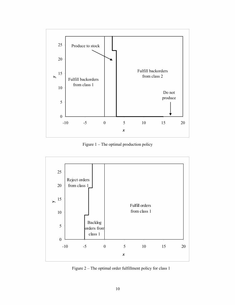
Optimal production policy

(P1) Produce to increase on-hand inventory if y = 0 and 0 ≤ x < or if y > 0 and 0 ≤ x < * (0)s * ( ).s y

(P2) Do not produce if y = 0 and x ≥ * (0).s

(P3) Produce to fulfill backorders from class 2 if y > 0 and * ( ).x s y≥

(P4) Produce to fulfill backorders from class 1 if x < 0.

(P5) It is never optimal to interrupt production once it has been initiated.

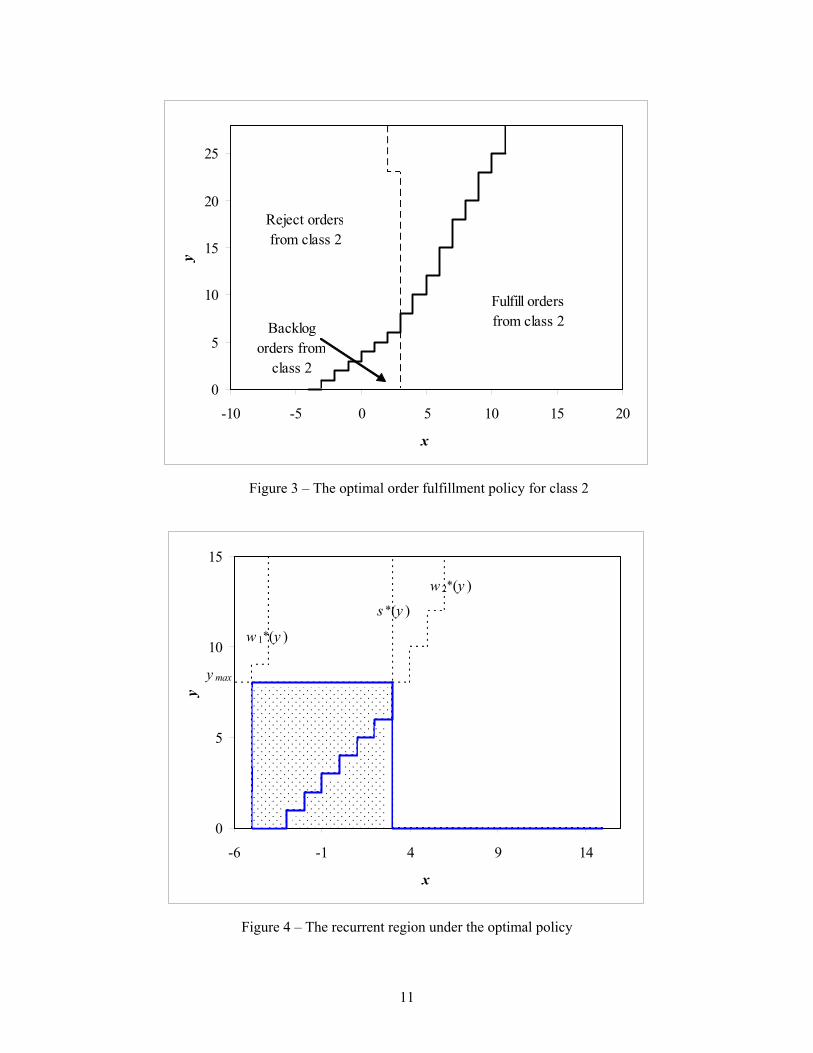
Optimal order fulfillment policy for class 1

(P6) Fulfill orders from class 1 from on-hand inventory if x > 0.

(P7) Backorder orders from class 1 if < x ≤ 0. *1 ( )w y

(P8) Reject orders from class 1 if x ≤ *1 ( ).w y

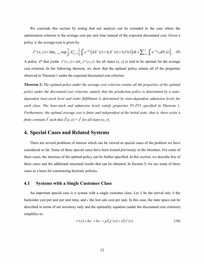
Optimal order fulfillment policy for class 2

(P9) Fulfill orders from class 2 from on-hand inventory if x > * ( 1)s y .+

8

(P10) Backorder orders from class 2 if < x ≤ *2 ( )w y * ( 1)s y .+

(P11) Reject orders from class 2 if x ≤ *2 ( ).w y

Moreover, the base-stock and admission levels have the following properties:

(P12) * ( )s y is non-increasing in y,

(P13) is non-decreasing in y, *1 ( )w y

(P14) is non-decreasing in y, and *2 ( )w y

(P15) and ≤ 0. * ( ) 0s y ≥ *1 ( )w y

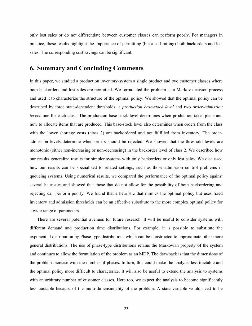
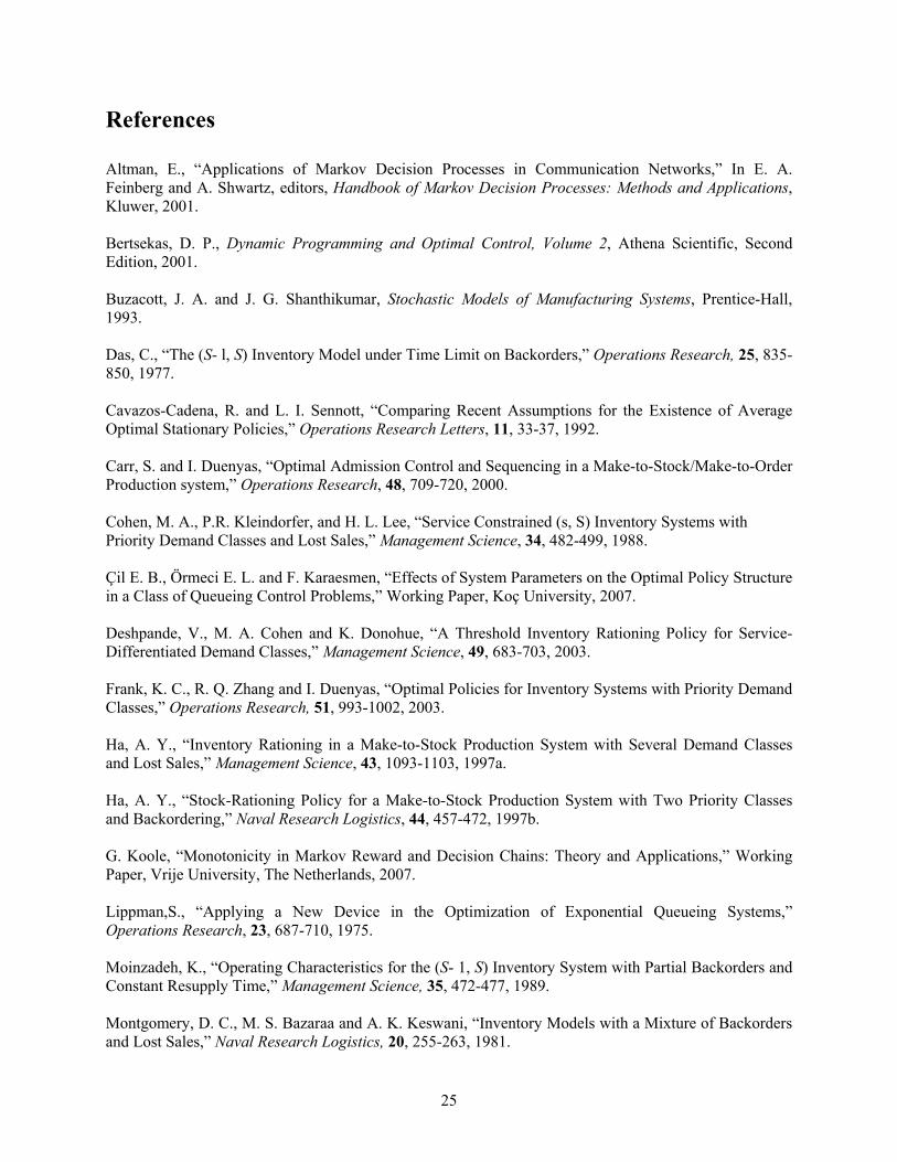
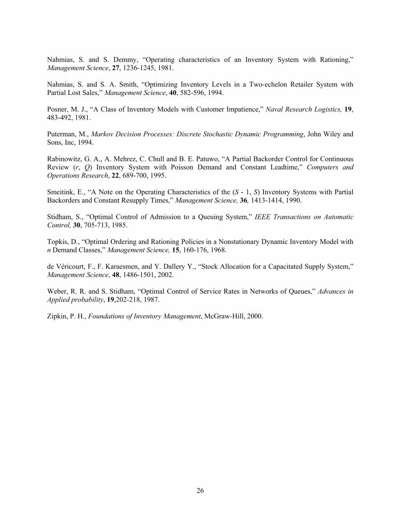
The optimal policy is illustrated for an example system (μ =0.50, λ1 =0.36, λ2 =0.21, c1 =357.00, c2

=186.00, b1 =4.80, b2 =0.50, h =1.50) in Figures 1-4. As we can see, the optimal policy defines several

regions in the state space where different combinations of order fulfillment and production decisions are

optimal. The contours of these regions are determined by the threshold functions * ( ),s y and

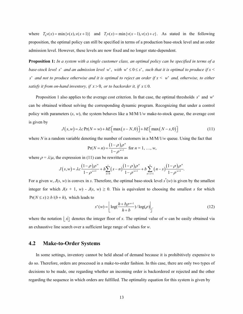
Note that only a subset of the state space is recurrent, and once the system enters the recurrent

region it never leaves it. Within the recurrent region the amount of on-hand inventory is always bounded

by and the amount of backorders from class 1 is always bounded by

*1 ( ),w y

*2 ( ).w y

* (0)s *1 (0).w− That is, we always

have Similarly, the amount of backorders from class 2 is always bounded in the

recurrent region. The maximum number of backorders of class 2 that may be allowed is given by

The recurrent region for the example system is shown in Figure 4.

*1 (0) (0).w x s≤ ≤ *

y* *max 2max{ : ( ) ( )}.y y s y w= =

In addition to placing limits on inventory and backorders, the optimal policy determines how

inventory is allocated among the two classes. The base-stock level * ( )s y can be viewed as an inventory

rationing parameter. If net inventory is below * ( ),s y then it is optimal to reserve inventory for future

orders from class 1 and to either reject or backorder orders from class 2. Similar rationing applies to

production, with priority given to increasing on-hand inventory over satisfying backorders from class 2 if

net inventory is below * ( 1)s y + .

In specifying the optimal policy, we chose in Theorem 1 to define the admission level for class 2 in

terms of a threshold on net inventory x. We could have equivalently chosen to define the

admission level in terms of a threshold on the number of backorders for class 2 (there exists a threshold

such that it is optimal to reject orders from class 2 if and to accept these orders

otherwise). The admission level is non-decreasing in x.

*2 ( )w y

* ( )r x * ( )y r x≥

* ( )r x

9

0

5

10

15

20

25

-10 -5 0 5 10 15 20

x

y

Fulfill backorders from class 2

Do notproduce

Fulfill backordersfrom class 1

Produce to stock

Figure 1 – The optimal production policy

0

5

10

15

20

25

-10 -5 0 5 10 15 20

x

y

Fulfill orders from class 1

Reject orders from class 1

Backlog orders from

class 1

Figure 2 – The optimal order fulfillment policy for class 1

10

0

5

10

15

20

25

-10 -5 0 5 10 15 20

x

y

Fulfill ordersfrom class 2Backlog

orders from class 2

Reject ordersfrom class 2

Figure 3 – The optimal order fulfillment policy for class 2

0

5

10

15

-6 -1 4 9 14

x

y

s *(y )

w 2*(y )

y max

w 1*(y )

Figure 4 – The recurrent region under the optimal policy

11

We conclude this section by noting that our analysis can be extended to the case where the

optimization criterion is the average cost per unit time instead of the expected discounted cost. Given a

policy π, the average-cost is given by:

( ){ }2( , ) 1 2 10 0

1( , ) lim sup ( ) ( ) ( ) ( ) .T Tt t

T x y i iiJ x y E e hX t b X t b Y t dt e c dN t

Tπ π α− + − −

→∞ == + + + ∑∫ ∫ α (9)

A policy π* that yields * ( , ) inf ( , )J x y J x yππ= for all states (x, y) is said to be optimal for the average

cost criterion. In the following theorem, we show that the optimal policy retains all of the properties

observed in Theorem 1 under the expected discounted cost criterion. Theorem 2: The optimal policy under the average cost criterion retains all the properties of the optimal

policy under the discounted cost criterion, namely that the production policy is determined by a state-

dependent base-stock level and order fulfillment is determined by state-dependent admission levels for

each class. The base-stock and admission levels satisfy properties P1-P15 specified in Theorem 1.

Furthermore, the optimal average cost is finite and independent of the initial state; that is, there exists a

finite constant J* such that J*(x, y) = J* for all states (x, y).

4. Special Cases and Related Systems

There are several problems of interest which can be viewed as special cases of the problem we have

considered so far. Some of these special cases have been treated previously in the literature. For some of

these cases, the structure of the optimal policy can be further specified. In this section, we describe few of

these cases and the additional structural results that can be obtained. In Section 5, we use some of these

cases as a basis for constructing heuristic policies.

4.1 Systems with a Single Customer Class

An important special case is a system with a single customer class. Let λ be the arrival rate, b the

backorder cost per unit per unit time, and c the lost sale cost per unit. In this case, the state space can be

described in terms of net inventory only and the optimality equation (under the discounted cost criterion)

simplifies to:

* *0 1( ) ( ) ( )v x hx bx T v x T v x*μ λ+ −= + + + (10)

12

where and 0 ( ) min{ ( ), ( 1)}T v x v x v x= + 1 ( ) min{ ( 1), ( ) }.T v x v x v x c= − + As stated in the following

proposition, the optimal policy can still be specified in terms of a production base-stock level and an order

admission level. However, these levels are now fixed and no longer state-dependent. Proposition 1: In a system with a single customer class, an optimal policy can be specified in terms of a

base-stock level *s and an admission level with * ,w * 0w * ,s≤ ≤ such that it is optimal to produce if x < *s and not to produce otherwise and it is optimal to reject an order if x < and, otherwise, to either

satisfy it from on-hand inventory, if or to backorder it, if

*w

0,x > 0.x ≤

Proposition 1 also applies to the average cost criterion. In that case, the optimal thresholds *s and

can be obtained without solving the corresponding dynamic program. Recognizing that under a control

policy with parameters (s, w), the system behaves like a M/M/1/w make-to-stock queue, the average cost

is given by

*w

( ) ( ) ( ), Pr( ) max ,0 max ,J s w c N w hE s N bE N sλ= = + ⎡ − ⎤ + ⎡ − 0 ⎤⎣ ⎦ ⎣ ⎦ (11)

where N is a random variable denoting the number of customers in a M/M/1/w queue. Using the fact that ( )

1

1Pr( )

1

n

wN nρ ρρ +

−= =

− for n = 1, …, w,

where ρ = λ/μ, the expression in (11) can be rewritten as

( ) ( ) ( ) ( ) ( ) ( )1 1

0 1

1 1, .

1 1

w ns w

w wn n s

J s w c h s n b n s 1

11

n

w

ρ ρ ρ ρλ

ρ ρ+ += = +

− −= + − + −

− −∑ ∑ρ ρρ +

−−

For a given w, J(s, w) is convex in s. Therefore, the optimal base-stock level s*(w) is given by the smallest

integer for which J(s + 1, w) - J(s, w) ≥ 0. This is equivalent to choosing the smallest s for which

Pr( ) /( ),N s b b h≤ ≥ + which leads to 1

*( ) log( ) / log( ) .wh bs w

h bρ ρ

++⎢ ⎥= ⎢ ⎥+⎣ ⎦ (12)

where the notation x⎢ ⎥⎣ ⎦ denotes the integer floor of x. The optimal value of w can be easily obtained via

an exhaustive line search over a sufficient large range of values for w.

4.2 Make-to-Order Systems

In some settings, inventory cannot be held ahead of demand because it is prohibitively expensive to

do so. Therefore, orders are processed in a make-to-order fashion. In this case, there are only two types of

decisions to be made, one regarding whether an incoming order is backordered or rejected and the other

regarding the sequence in which orders are fulfilled. The optimality equation for this system is given by

13

* * *1 2 0 1 1 2 2( , ) ( , ) ( , ) ( , ),v x y b x b y T v x y T v x y T v x y*μ λ λ−= + + + + (13)

where the operators Ti, i = 0, 1, 2, are defined as follows:

{ }{ }{ }0

min ( , ), ( 1, ), ( , 1) if 0 and 0min ( , ), ( , 1) if 0 and 0

( , )min ( , ), ( 1, ) if 0 and 0( , ) if 0 and 0,

v x y v x y v x y x yv x y v x y x y

T v x yv x y v x y x y

v x y x y

⎧ + − <⎪

>

− = >= ⎨

+ < =

= =

⎪

⎪⎪⎩

(14)

{ }1 ( , ) min ( 1, ), ( , ) ,T v x y v x y v x y c= − + 1 (15)

and { }2 ( , ) min ( , 1), ( , ) .T v x y v x y v x y c= + + 2 (16)

Noting that it is never optimal not to produce whenever there is a backorder from either class 1 or class 2,

operator T0 can be further simplified as

{ }

0

min ( 1, ), ( , 1) if 0 and 0( , 1) if 0 and 0

( , )( 1, ) if 0 and 0( , ) if 0 and 0,

v x y v x y x yv x y x y

T v x yv x y x yv x y x y

⎧ + − <⎪

>− = >⎪= ⎨

+ < =⎪⎪ = =⎩

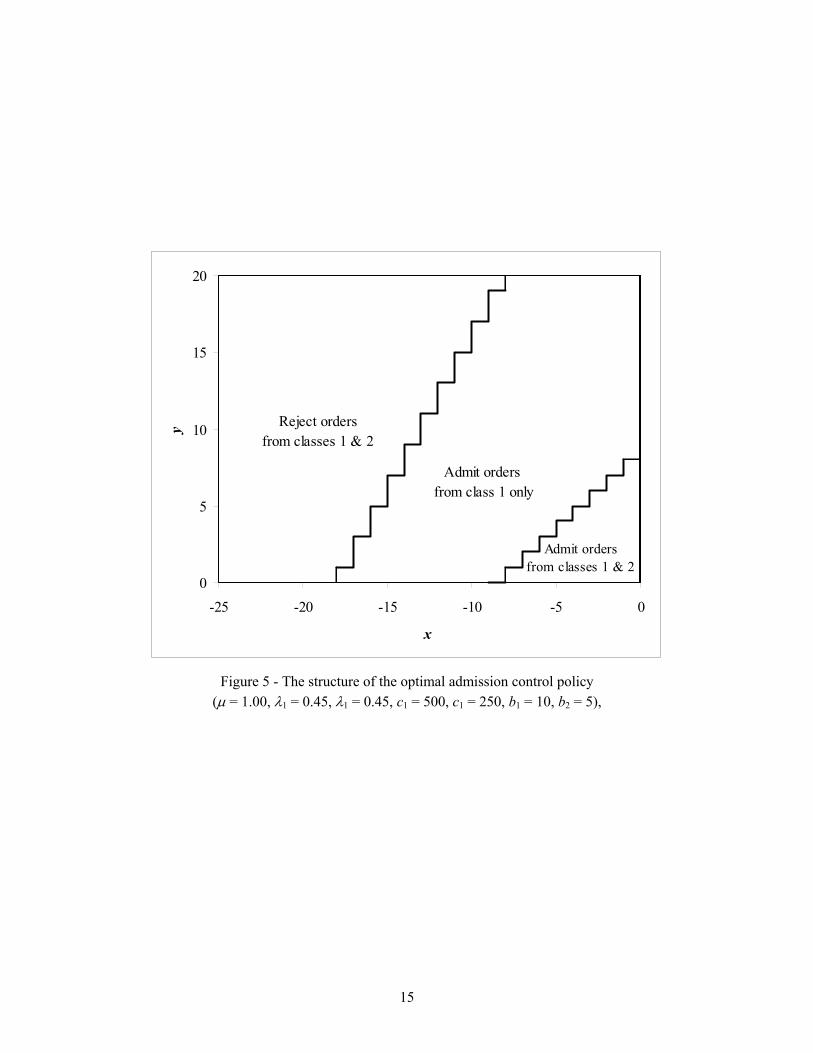
As described in the following proposition (we omit the proof for the sake of brevity), and illustrated

in Figure 5, the optimal policy can be described in terms of two state-dependent admission levels w1(y)

and w2(y). Proposition 2: In a make-to-order system, an optimal policy can be specified in terms of two state-

dependent admission levels and such that it is optimal to admit orders from class i if

< x, for i = 1, 2, and to reject the orders otherwise. Moreover, for i = 1, 2 is non-decreasing

in y.

*1 ( ),w y *

2 ( )w y

* ( )iw y * ( )iw y

Make-to-order systems have been studied in the literature in the context of optimal queue admission

control. Although that literature is extensive, most of it deals with single class systems or systems where

the backordering (delay) costs are the same for all the customer classes. In the case where the backorder

costs are identical, b1 = b2, the problem simplifies significantly (the state space can be described by the

variable x only) and the optimal policy is specified by fixed admission levels (see Stidham 1988 for an

early reference and Çil et al. (2007) for related discussion). To our knowledge, the results described in

proposition 2 are new to the admission control literature.

14

0

5

10

15

20

-25 -20 -15 -10 -5

x

y

0

Reject ordersfrom classes 1 & 2

Admit ordersfrom classes 1 & 2

Admit orders from class 1 only

Figure 5 - The structure of the optimal admission control policy

(μ = 1.00, λ1 = 0.45, λ1 = 0.45, c1 = 500, c1 = 250, b1 = 10, b2 = 5),

15

4.3 Other Special Cases

There are other problems with two customer classes that have been studied previously in the literature and

that can be viewed as special cases of our problem. For example, in settings where backorders are not

allowed, with orders either fulfilled from on-hand inventory or rejected, the optimal production policy can

be shown (by suitably modifying the operators T0, T1, and T2) to be characterized by a fixed base-stock

level that determines whether or not production takes place and a fixed inventory rationing level that

determines whether orders from class 2 are fulfilled from on-hand inventory or rejected; see Ha (1997a)

for details. Similarly, for systems where lost sales are not allowed and all orders must be either fulfilled

from on-hand inventory or backordered, the optimal policy consists of a fixed production base-stock level

and a fixed inventory rationing level; see Ha (1997b) for a discussion of systems with two classes and de

Véricourt et al. (2002) for generalization to systems with multiple classes. We will revisit these two

models in Section 5 on heuristics.

Other variations that can be studied using our framework include hybrid make-to-order/make-to-stock

systems where on-hand inventory is always reserved for one class (the make-to-stock class) while the

other class is always either backordered or rejected (the make-to-order class). Carr and Duenyas (2000)

study the case where orders from the make-to-stock class must be rejected if no on-hand inventory is

available. For this case, the optimality equation simplifies as follows:

* * *2 0 1 1 2 2( , ) ( , ) ( , ) ( , ),v x y hx b y T v x y T v x y T v x y*μ λ λ= + + + + (17)

where the operators Ti are now defined as follows:

{ }{ }0

min ( , ), ( 1, ), ( , 1) if 0( , )

min ( , ), ( 1, ) if 0,v x y v x y v x y y

T v x yv x y v x y y

⎧ + −⎪= ⎨>

+ =⎪⎩ (18)

11

( 1, ) if 0 ( , )

( , ) , otherwise, v x y x

T v x yv x y c

− >⎧= ⎨ +⎩

(19)

and { }2 ( , ) min ( , 1), ( , ) .T v x y v x y v x y c= + + 2 (20)

Note that x now denotes on-hand inventory since no backorders from class 1 are allowed. Also note that

there are no decisions associated with operator T1 since orders from class 1 cannot be backordered.

Similarly, decisions associated with operator T2 are limited to either backordering or rejecting orders from

class 2 since orders from class 2 cannot be fulfilled from on-hand inventory. Consequently, the optimal

policy is specified by two state-dependent thresholds s(y) and w(y) such that it is optimal to produce to

increase on-hand inventory if x < s(y), where s(y) is decreasing in y, fulfill backorders from class 2 if x≥

16

s(y) and y > 0, and admit orders from class 2 if x > w(y), where w(y) is increasing in y. This problem is

obviously simpler than the one with which we deal in this paper since there is no inventory allocation

between the two classes and there is no problem of production sequencing, which arises when both

classes are backordered.

5. Heuristics

In this section, we compare the performance of four plausible heuristics against the performance of the

optimal policy for the general problem described in Sections 2 and 3. Our aim is to assess the benefit of

using the optimal policy instead of simpler heuristics. We focus on heuristics that involve fixed (non-state

dependent) parameters since they are simpler to communicate and implement and, perhaps, are more

common in practice. Below we provide a description of each of the heuristics we consider. Heuristic H1: Under heuristic H1, no rejection is allowed and all orders are either fulfilled from on-hand

inventory or backordered. The heuristic specifies two fixed thresholds, a base-stock level H1s and an

inventory rationing level Hr he production facility produces if 1. T H1x s< and otherwise it does not. Orders

from class 1 are always fulfilled from on-hand inventory, if any is available, and otherwise are

backordered. Orders from class 2 are fulfilled from on-hand inventory if H1x r≥ and otherwise are

backordered. When there are backorders from both classes, priority is given to orders from class 1.

Backorders from class 2 are fulfilled if H1x r≥ . As we discussed in Section 4.3, this policy is optimal

when rejection is not allowed. Optimal values for the parameters H1s and can be obtained in closed

form using the approach described in de Véricourt et al. (2002).

H1r

Heuristic H2: Under Heuristic H2, no backorders are allowed. Orders from both classes are either

fulfilled from on-hand inventory or rejected. Similar to H1, heuristic H2 specifies two fixed thresholds, a

base-stock level H2s and an inventory rationing level The production facility produces if H2.r H2x s< and

otherwise it does not. Orders from class 1 are always fulfilled from on-hand inventory, if any is available,

and otherwise are rejected. Orders from class 2 are fulfilled from on-hand inventory if H2x r≥ and

otherwise are rejected. Ha (1997b) describes a search procedure for determining the optimal values for the

parameters H2s and using closed form expressions for the average cost. H2r Heuristic H3: Heuristic H3 allows for both backordering and rejection. The heuristic specifies two

thresholds H3s and . The production facility produces if H3w H3x s< and does not produce otherwise.

17

Orders from both classes are either fulfilled from on-hand inventory, if any is available, on a first-come,

first-served basis (FCFS) or backordered if H3.x w> Orders are rejected regardless of class if H3.x w≤ In

contrast to H1 and H2, H3 does not differentiate between the two classes and orders from both classes are

fulfilled on a first-come, first serve basis. This system can be analyzed using the single product model of

Section 4.1 by letting and with 2

1 i iib p

== ∑ b c2

1 i iic p

== ∑ 1 2/( ).i ip λ λ λ= + The value of the parameters

H3s and can be obtained using the approach described in that section. H3w Heuristic H4: Similar to H3, heuristic H4 allows for both backordering and rejection. However, the

heuristic differentiates between the two classes. To do so, H4 specifies four fixed thresholds

The production facility produces if H4 4 H4,1 H4,2, , , and .Hs r w w H4x s< and otherwise does not. Orders from

class 1 are either fulfilled from on-hand inventory or backordered if Otherwise, they are

rejected. Orders from class 2 are fulfilled from on hand-hand inventory if

H4,1.x w>

H4.x r≥ They are backordered if

and are otherwise rejected. If both classes are backordered, the production facility produces first

to fulfill backorders from class 1, then to increase on-hand inventory up to then to fulfill backorders

from class 2 when

H4,2y w≤

H4 ,r

H4.x r≥ Heuristic H4 mimics the optimal policy. The thresholds

H4 H4 H4,1 H4,2, , , and s r w w play similar roles to 1

* * * *(0), s ( ), (y), and ( )2

s y w w y under the optimal policy. An

important difference is of course the fact that the thresholds in H4 are not state-dependent but are instead

fixed.

The average cost under the above heuristic for a given choice of the parameters

can be computed using the following dynamic programming equation H4 4 H4,1 H4,2, , , and Hs r w w

* H4 H4H4 1 2 0 1 1 2 2( , ) ( , ) ( , ) ( , ),v x y J hx b x b y T v x y T v x y T v x yH4μ λ λ+ −+ = + + + + +

where

4H4

0 4

H4

( 1, ) if ( , ) ( 1, ) if and 0

( , 1) if and 0,

H

H

v x y x rT v x y v x y x s y

v x y x r y

+ <⎧⎪= + <⎨⎪

=− ≥ >⎩

H4,1H41

1

( 1, ) if ,( , )

( , ) otherwise,v x y x w

T v x yv x y c

− >⎧= ⎨ +⎩

and

H4 H4,2H4

2 H

2 4,2

( 1, ) if and ( , ) ( , 1) if and

( , ) if .H

v x y x r y wT v x y v x y x r y w

v x y c y w

⎧ − ≥⎪= + < <⎨⎪ + ≥⎩

4 H4,2

<

18

The optimal parameters can be obtained using an exhaustive grid search. This search which can be

extensive is facilitated by taking advantage of the fact that H4,1 H4 H40 .w r s≤ ≤ ≤

To test the performance of the heuristics against that of the optimal policy, we carried out a series of

numerical experiments for systems with a wide range of parameter values. For the optimal policy (also for

heuristic H4), numerical results are obtained by solving the corresponding dynamic programming

equation using the value iteration method. The value iteration algorithm we use is a direct adaptation of

the algorithm described in Puterman (Chapter 8, 1994). The state space is truncated at

where min max max{ , } {0,x x y− × } min max max, , and x x y are positive integers that are gradually increased until

the cost is no longer sensitive to the truncation level. The value iteration algorithm is terminated once

five-digit accuracy is obtained. For heuristics H1-H4, we use the procedures described above to determine

the corresponding optimal combination of control parameters. For heuristic H4, we limited the search for

these parameters using the recurrent region for the optimal policy. This appears to be sufficient to support

the conclusions we draw regarding the performance of H4. However, the performance of H4 may

potentially improve with a more exhaustive search. For each scenario we tested, we obtain the average

cost under the optimal policy *J and the average cost under each of the heuristics *HiJ for i = 1, …, 4 and

then compute the percentage difference between the cost of the optimal policy and the cost of each

heuristic, * *H( ) /i

*.J J J− We use the average cost criterion, instead of discounted cost, in our comparisons

because the results are independent of the starting state and of the discount factor.

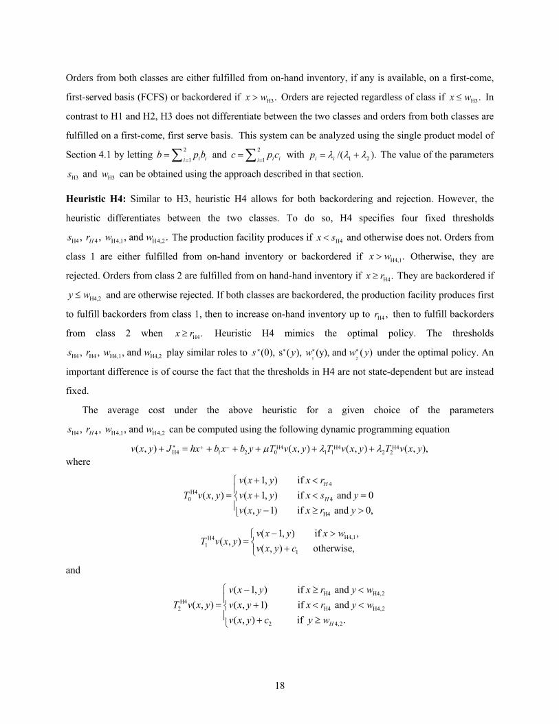
Representative results are shown in Figures 6-9. Based on these results, the following observations

can be made.

• Heuristic H4 outperforms all other heuristics. The percentage cost difference between H4 and the

optimal policy is generally small, with less than 5% in most of the cases tested. In contrast, all other

heuristics can perform poorly for certain combinations of parameter values.

• For H1, performance deteriorates when the backorder cost for one (or both) classes is high; see Figure

6. This is consistent with intuition. Heuristic H1 does not have the option of limiting the number of

backorders when backorder costs are high without increasing inventory. Consequently, cost can grow

arbitrarily large with increases in backorder costs.

19

0%

5%

10%

15%

20%

25%

30%

35%

40%

1 21 41 61 81

b1/b2

Perc

enta

ge c

ost d

iffer

ence H1 H2

H3 H4

Figure 6 – The effect of backorder costs on the performance of heuristics (μ = 1, λ1 = 0.4, λ2 = 0.5, c1 =

500, c1 = 250, h = 1, b2 = 5)

0%

10%

20%

30%

40%

50%

60%

70%

80%

1 5 9 13

c 1/c 2

Perc

enta

ge c

ost d

iffer

ence

H1 H2H3 H4

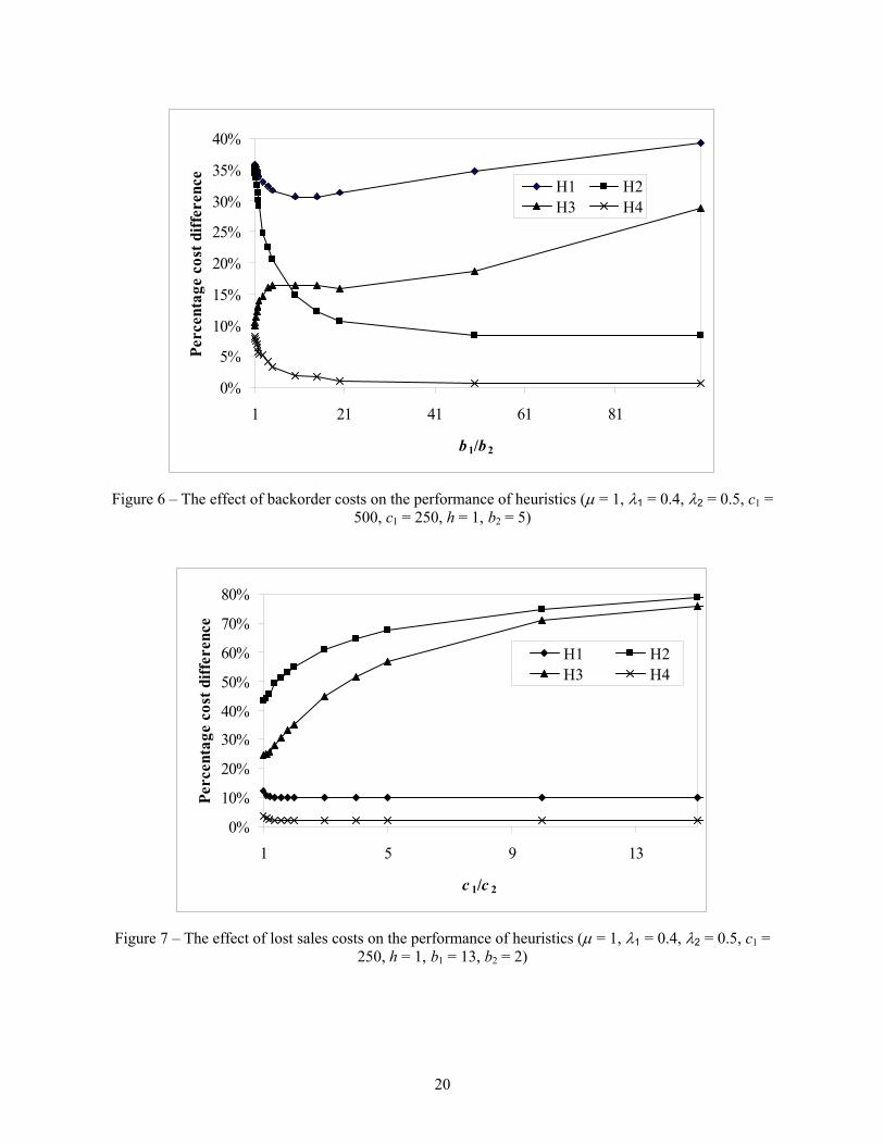
Figure 7 – The effect of lost sales costs on the performance of heuristics (μ = 1, λ1 = 0.4, λ2 = 0.5, c1 =

250, h = 1, b1 = 13, b2 = 2)

20

0%

30%

60%

90%

120%

150%

180%

210%

0 1 2 3 4 5 6 7 8 9 1

h

Perc

enta

ge c

ost d

iffer

ence

0

H1 H2H3 H4

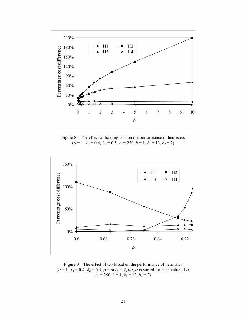
Figure 8 – The effect of holding cost on the performance of heuristics (μ = 1, λ1 = 0.4, λ2 = 0.5, c2 = 250, h = 1, b1 = 13, b2 = 2)

0%

50%

100%

150%

0.6 0.68 0.76 0.84 0.92

ρ

Perc

enta

ge c

ost d

iffer

ence H1 H2

H3 H4

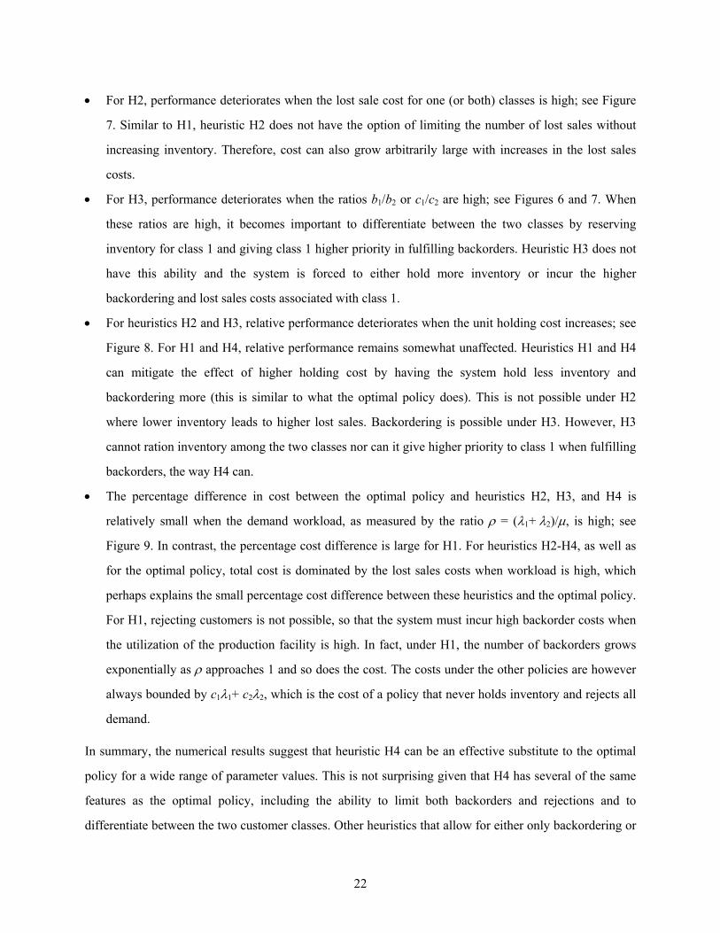
Figure 9 – The effect of workload on the performance of heuristics (μ = 1, λ1 = 0.4, λ2 = 0.5, ρ = α(λ1 + λ2)/μ, α is varied for each value of ρ,

c1 = 250, h = 1, b1 = 13, b2 = 2)

21

• For H2, performance deteriorates when the lost sale cost for one (or both) classes is high; see Figure

7. Similar to H1, heuristic H2 does not have the option of limiting the number of lost sales without

increasing inventory. Therefore, cost can also grow arbitrarily large with increases in the lost sales

costs.

• For H3, performance deteriorates when the ratios b1/b2 or c1/c2 are high; see Figures 6 and 7. When

these ratios are high, it becomes important to differentiate between the two classes by reserving

inventory for class 1 and giving class 1 higher priority in fulfilling backorders. Heuristic H3 does not

have this ability and the system is forced to either hold more inventory or incur the higher

backordering and lost sales costs associated with class 1.

• For heuristics H2 and H3, relative performance deteriorates when the unit holding cost increases; see

Figure 8. For H1 and H4, relative performance remains somewhat unaffected. Heuristics H1 and H4

can mitigate the effect of higher holding cost by having the system hold less inventory and

backordering more (this is similar to what the optimal policy does). This is not possible under H2

where lower inventory leads to higher lost sales. Backordering is possible under H3. However, H3

cannot ration inventory among the two classes nor can it give higher priority to class 1 when fulfilling

backorders, the way H4 can.

• The percentage difference in cost between the optimal policy and heuristics H2, H3, and H4 is

relatively small when the demand workload, as measured by the ratio ρ = (λ1+ λ2)/μ, is high; see

Figure 9. In contrast, the percentage cost difference is large for H1. For heuristics H2-H4, as well as

for the optimal policy, total cost is dominated by the lost sales costs when workload is high, which

perhaps explains the small percentage cost difference between these heuristics and the optimal policy.

For H1, rejecting customers is not possible, so that the system must incur high backorder costs when

the utilization of the production facility is high. In fact, under H1, the number of backorders grows

exponentially as ρ approaches 1 and so does the cost. The costs under the other policies are however

always bounded by c1λ1+ c2λ2, which is the cost of a policy that never holds inventory and rejects all

demand. In summary, the numerical results suggest that heuristic H4 can be an effective substitute to the optimal

policy for a wide range of parameter values. This is not surprising given that H4 has several of the same

features as the optimal policy, including the ability to limit both backorders and rejections and to

differentiate between the two customer classes. Other heuristics that allow for either only backordering or

22

only lost sales or do not differentiate between customer classes can perform poorly. For managers in

practice, these results highlight the importance of permitting (but also limiting) both backorders and lost

sales. The corresponding cost savings can be significant.

6. Summary and Concluding Comments

In this paper, we studied a production inventory-system a single product and two customer classes where

both backorders and lost sales are permitted. We formulated the problem as a Markov decision process

and used it to characterize the structure of the optimal policy. We showed that the optimal policy can be

described by three state-dependent thresholds: a production base-stock level and two order-admission

levels, one for each class. The production base-stock level determines when production takes place and

how to allocate items that are produced. This base-stock level also determines when orders from the class

with the lower shortage costs (class 2) are backordered and not fulfilled from inventory. The order-

admission levels determine when orders should be rejected. We showed that the threshold levels are

monotonic (either non-increasing or non-decreasing) in the backorder level of class 2. We described how

our results generalize results for simpler systems with only backorders or only lost sales. We discussed

how our results can be specialized to related settings, such as those admission control problems in

queueing systems. Using numerical results, we compared the performance of the optimal policy against

several heuristics and showed that those that do not allow for the possibility of both backordering and

rejecting can perform poorly. We found that a heuristic that mimics the optimal policy but uses fixed

inventory and admission thresholds can be an effective substitute to the more complex optimal policy for

a wide range of parameters.

There are several potential avenues for future research. It will be useful to consider systems with

different demand and production time distributions. For example, it is possible to substitute the

exponential distribution by Phase-type distributions which can be constructed to approximate other more

general distributions. The use of phase-type distributions retains the Markovian property of the system

and continues to allow the formulation of the problem as an MDP. The drawback is that the dimensions of

the problem increase with the number of phases. In turn, this could make the analysis less tractable and

the optimal policy more difficult to characterize. It will also be useful to extend the analysis to systems

with an arbitrary number of customer classes. Here too, we expect the analysis to become significantly

less tractable because of the multi-dimensionality of the problem. A state variable would need to be

23

associated with the backorder from each class. Nevertheless, we expect the structure of the optimal policy

to remain the same with inventory rationing and admission thresholds associated with each customer

class. These thresholds would now be dependent on the vector of backorder levels from all the classes.

24

References

Altman, E., “Applications of Markov Decision Processes in Communication Networks,” In E. A. Feinberg and A. Shwartz, editors, Handbook of Markov Decision Processes: Methods and Applications, Kluwer, 2001. Bertsekas, D. P., Dynamic Programming and Optimal Control, Volume 2, Athena Scientific, Second Edition, 2001. Buzacott, J. A. and J. G. Shanthikumar, Stochastic Models of Manufacturing Systems, Prentice-Hall, 1993. Das, C., “The (S- l, S) Inventory Model under Time Limit on Backorders,” Operations Research, 25, 835-850, 1977. Cavazos-Cadena, R. and L. I. Sennott, “Comparing Recent Assumptions for the Existence of Average Optimal Stationary Policies,” Operations Research Letters, 11, 33-37, 1992. Carr, S. and I. Duenyas, “Optimal Admission Control and Sequencing in a Make-to-Stock/Make-to-Order Production system,” Operations Research, 48, 709-720, 2000. Cohen, M. A., P.R. Kleindorfer, and H. L. Lee, “Service Constrained (s, S) Inventory Systems with Priority Demand Classes and Lost Sales,” Management Science, 34, 482-499, 1988. Çil E. B., Örmeci E. L. and F. Karaesmen, “Effects of System Parameters on the Optimal Policy Structure in a Class of Queueing Control Problems,” Working Paper, Koç University, 2007. Deshpande, V., M. A. Cohen and K. Donohue, “A Threshold Inventory Rationing Policy for Service- Differentiated Demand Classes,” Management Science, 49, 683-703, 2003. Frank, K. C., R. Q. Zhang and I. Duenyas, “Optimal Policies for Inventory Systems with Priority Demand Classes,” Operations Research, 51, 993-1002, 2003. Ha, A. Y., “Inventory Rationing in a Make-to-Stock Production System with Several Demand Classes and Lost Sales,” Management Science, 43, 1093-1103, 1997a. Ha, A. Y., “Stock-Rationing Policy for a Make-to-Stock Production System with Two Priority Classes and Backordering,” Naval Research Logistics, 44, 457-472, 1997b. G. Koole, “Monotonicity in Markov Reward and Decision Chains: Theory and Applications,” Working Paper, Vrije University, The Netherlands, 2007. Lippman,S., “Applying a New Device in the Optimization of Exponential Queueing Systems,” Operations Research, 23, 687-710, 1975. Moinzadeh, K., “Operating Characteristics for the (S- 1, S) Inventory System with Partial Backorders and Constant Resupply Time,” Management Science, 35, 472-477, 1989. Montgomery, D. C., M. S. Bazaraa and A. K. Keswani, “Inventory Models with a Mixture of Backorders and Lost Sales,” Naval Research Logistics, 20, 255-263, 1981.

25

Nahmias, S. and S. Demmy, “Operating characteristics of an Inventory System with Rationing,” Management Science, 27, 1236-1245, 1981. Nahmias, S. and S. A. Smith, “Optimizing Inventory Levels in a Two-echelon Retailer System with Partial Lost Sales,” Management Science, 40, 582-596, 1994. Posner, M. J., “A Class of Inventory Models with Customer Impatience,” Naval Research Logistics, 19, 483-492, 1981. Puterman, M., Markov Decision Processes: Discrete Stochastic Dynamic Programming, John Wiley and Sons, Inc, 1994. Rabinowitz, G. A., A. Mehrez, C. Chull and B. E. Patuwo, “A Partial Backorder Control for Continuous Review (r, Q) Inventory System with Poisson Demand and Constant Leadtime,” Computers and Operations Research, 22, 689-700, 1995. Smeitink, E., “A Note on the Operating Characteristics of the (S - 1, S) Inventory Systems with Partial Backorders and Constant Resupply Times,” Management Science, 36, 1413-1414, 1990. Stidham, S., “Optimal Control of Admission to a Queuing System,” IEEE Transactions on Automatic Control, 30, 705-713, 1985. Topkis, D., “Optimal Ordering and Rationing Policies in a Nonstationary Dynamic Inventory Model with n Demand Classes,” Management Science, 15, 160-176, 1968. de Véricourt, F., F. Karaesmen, and Y. Dallery Y., “Stock Allocation for a Capacitated Supply System,” Management Science, 48, 1486-1501, 2002. Weber, R. R. and S. Stidham, “Optimal Control of Service Rates in Networks of Queues,” Advances in Applied probability, 19,202-218, 1987. Zipkin, P. H., Foundations of Inventory Management, McGraw-Hill, 2000.

26

Appendix2

The following notation is used throughout this appendix:

( , ) ( 1, ) ( , ),xv x y v x y v x yΔ = + −

( , ) ( , 1) ( , ),yv x y v x y v x yΔ = + −

, ( , ) ( 1, ) ( , ),x x x xv x y v x y v x yΔ = Δ + − Δ

, ( , ) ( , 1) ( , ),y y y yv x y v x y v x yΔ = Δ + − Δ and

, ,( , ) ( , ) ( 1, ) ( , ).x y y x y yv x y v x y v x y v x yΔ = Δ = Δ + − Δ

Proof of Lemma 1 To show that Tv ∈V, it is sufficient to show that Tiv ∈V for i = 0, 1, and 2. Therefore, we divide the

proof into three parts. In part 1, we prove that if v∈V then T1v ∈V. In part 2, we prove that if v∈V then

T2v ∈V. In part 3, we prove that if v∈V then T0v ∈V. In doing so, we will show that Tiv, for i = 0, 1 and 2,

satisfies properties A1-A8.

Before proceeding with the proof, let us note that properties A3 and A4 are implied by properties A5,

A6 and A7. Using A5 and A6, we have ( 1, ) ( 1, 1) ( , )x x xv x y v x y v x yΔ + ≥ Δ + + ≥ Δ . Hence, and

A3 holds. Also, using A5 and A7, we have

, ( , ) 0x xv x yΔ ≥

( , 1) ( 1, 1) ( , )y y yv x y v x y v x yΔ + ≥ Δ + + ≥ Δ . Hence,

and A4 holds. Consequently, in what follows, we only need to show that T

, ( , ) 0y yv x yΔ ≥

iv satisfies properties A1, A2

and A5-A8 for i = 0, 1 and 2.

Operator T1

We need to show that satisfies A1-A2 and A5-A8. 1T v Property A1

For x < 0 and y > 0, we have Then, ( 1, ) ( , 1).v x y v x y+ ≤ −

( )( )

1 1

1

1

1

( 1, ) min{ ( , ), ( 1, ) }min{ ( , ), ( , 1) } using the fact that ( 1, ) ( , 1)

min{ ( 1, 1), ( , 1) } using the fact that ( , ) ( 1, 1)( , 1).

T v x y v x y v x y cv x y v x y c v x y v x y

v x y v x y c v x y v x yT v x y

+ = + +

≤ − + + ≤ −

≤ − − − + ≤ − −

= −

For x<0 and , we also have . Then, 0y ≥ ( 1, ) ( , )v x y v x y+ ≤

2 Should the paper be published, it would be appropriate to place this appendix in an online companion to the paper.

27

( )( )

1 1

1

1

1

( 1, ) min{ ( , ), ( 1, ) }min{ ( 1, ), ( 1, ) } using the fact ( , ) ( 1, )

min{ ( 1, ), ( , ) } using the fact ( 1, ) ( , )( , ).

T v x y v x y v x y cv x y v x y c v x y v x y

v x y v x y c v x y v x yT v x y

+ = + +

≤ − + + ≤ −

≤ − + + ≤

=

Hence, satisfies A1. 1T v Property A2

For y>0, we have . Then, ( , 1) ( , )v x y v x y− ≤

( )( )

1 1

1

1

1

( , 1) min{ ( 1, 1), ( , 1) }min{ ( 1, 1), ( , ) } using the fact ( , 1) ( , )

min{ ( 1, ), ( , ) } using the fact ( 1, 1) ( 1, )( , ).

T v x y v x y v x y cv x y v x y c v x y v x y

v x y v x y c v x y v x yT v x y

− = − − − +

≤ − − + − ≤

≤ − + − − ≤ −

=

Hence, satisfies A2. 1T v Property A5

First note that

{ }{

1

1

( , ) min ( 1, ), ( , )

( 1, ) min 0, ( 1, )x

T v x y v x y v x y c

v x y v x y c

= − +

= − + Δ − + }1

. (1)

Then

{ } { }{ } {

, 1 , 1 1

1 1

( , ) ( 1, ) min 0, ( , 1) min 0, ( , )

min 0, ( 1, 1) min 0, ( 1, ) .x y x y x x

x x

T v x y v x y v x y c v x y c

v x y c v x y c

Δ = Δ − + Δ + + − Δ

− Δ − + + + Δ − + }+

1

Using A3, A5 and A6, we have .

Hence, we distinguish the following cases.

1 1 1( , ) ( , 1) ( 1, ) ( 1, 1)x x x xv x y c v x y c v x y c v x y cΔ + ≥ Δ + + ≥ Δ − + ≥ Δ − + +

Case 1: 1 1 1 1( , ) ( , 1) ( 1, ) ( 1, 1) 0x x x xv x y c v x y c v x y c v x y cΔ + ≥ Δ + + ≥ Δ − + ≥ Δ − + + ≥ ⇒

≤, 1 ,( , ) ( 1, ) 0x y x yT v x y v x yΔ = Δ − (using A5).

Case 2: 1 1 1 1( , ) ( , 1) ( 1, ) 0 ( 1, 1)x x x xv x y c v x y c v x y c v x y cΔ + ≥ Δ + + ≥ Δ − + ≥ ≥ Δ − + + ⇒

≤, 1 1( , ) ( 1, ) 0x y xT v x y v x y cΔ = −Δ − − .

Case 3: 1 1 1 1( , ) ( , 1) 0 ( 1, ) ( 1, 1)x x x xv x y c v x y c v x y c v x y cΔ + ≥ Δ + + ≥ ≥ Δ − + ≥ Δ − + + ⇒

, 1 ( , ) 0x yT v x yΔ = .

Case 4: 1 1 1 1( , ) 0 ( , 1) ( 1, ) ( 1, 1)x x x xv x y c v x y c v x y c v x y cΔ + ≥ ≥ Δ + + ≥ Δ − + ≥ Δ − + + ⇒

≤, 1 1( , ) ( , 1) 0x y xT v x y v x y cΔ = Δ + + .

Case 5: 1 1 1 10 ( , ) ( , 1) ( 1, ) ( 1, 1)x x x xv x y c v x y c v x y c v x y c≥ Δ + ≥ Δ + + ≥ Δ − + ≥ Δ − + + ⇒

28

, 1 ,( , ) ( , ) 0x y x yT v x y v x yΔ = Δ ≤ (using A5).

Since for all possible cases we have satisfies A5. , 1 ( , ) 0,x yT v x yΔ ≤ 1 ( , )T v x y

Property A6

Property A6 can be rewritten as follows

( 2, ) ( 1, 1) ( 1, ) ( , 1) ( 1, ) ( , 1)x xv x y v x y v x y v x y v x y v x y+ − + − − + + − = Δ + − Δ − ≥ 0 .

Then, using (1), we have

{ }{ } { } {

1 1 1

1 1

( 1, ) ( , 1) ( , ) ( 1, 1) min 0, ( 1, )

min 0, ( , 1) min 0, ( , ) min 0, ( 1, 1) .x x x x x

x x x

T v x y T v x y v x y v x y v x y c

v x y c v x y c v x y c

Δ + − Δ − = Δ − Δ − − + Δ + +

− Δ − + − Δ + + Δ − − + }1

1

Using A5 and A6, we have .

Hence, we distinguish the following 5 possible cases.

1 1 1( 1, 1) ( , ) ( , 1) ( 1, )x x x xv x y c v x y c v x y c v x y cΔ − − + ≤ Δ + ≤ Δ − + ≤ Δ + +

Case 1: 1 1 1 10 ( 1, 1) ( , ) ( , 1) ( 1, )x x x xv x y c v x y c v x y c v x y c≤ Δ − − + ≤ Δ + ≤ Δ − + ≤ Δ + + ⇒

1 1( 1, ) ( , 1) ( , ) ( 1, 1) 0x x x xT v x y T v x y v x y v x yΔ + − Δ − = Δ − Δ − − ≥ .

Case 2: 1 1 1 1( 1, 1) 0 ( , ) ( , 1) ( 1, )x x x xv x y c v x y c v x y c v x y cΔ − − + ≤ ≤ Δ + ≤ Δ − + ≤ Δ + + ⇒

1 01 1( 1, ) ( , 1) ( , )x x xT v x y T v x y v x y cΔ + − Δ − = Δ + ≥ .

Case 3: 1 1 1 1( 1, 1) ( , ) 0 ( , 1) ( 1, )x x x xv x y c v x y c v x y c v x y cΔ − − + ≤ Δ + ≤ ≤ Δ − + ≤ Δ + + ⇒

1 1( 1, ) ( , 1) 0x xT v x y T v x yΔ + − Δ − = .

Case 4: 1 1 1 1( 1, 1) ( , ) ( , 1) 0 ( 1, )x x x xv x y c v x y c v x y c v x y cΔ − − + ≤ Δ + ≤ Δ − + ≤ ≤ Δ + + ⇒

11 1( 1, ) ( , 1) ( , 1) 0x x xT v x y T v x y v x y cΔ + − Δ − = −Δ − − ≥ .

Case 5: 1 1 1 1( 1, 1) ( , ) ( , 1) ( 1, ) 0x x x xv x y c v x y c v x y c v x y cΔ − − + ≤ Δ + ≤ Δ − + ≤ Δ + + ≤ ⇒

1 1( 1, ) ( , 1) ( 1, ) ( , 1) 0x x x xT v x y T v x y v x y v x yΔ + − Δ − = Δ + − Δ − ≥ .

Since for all possible cases , satisfies A6. 1 1( 1, ) ( , 1) 0x xT v x y T v x yΔ + − Δ − ≥ 1 ( , )T v x y Property A7

Property 7 can be rewritten as follows

( 1, 1) ( , ) ( 1, ) ( , 1) ( 1, ) ( , 1)y yv x y v x y v x y v x y v x y v x y+ + − − + + − = Δ + − Δ − ≥ 0 .

Then, using (1), we have

{ }{ } { } {

1 1 1

1 1

( 1, ) ( , 1) ( , ) ( 1, 1) min 0, ( , 1)

min 0, ( 1, ) min 0, ( , ) min 0, ( 1, 1) .y y y y x

x x x

T v x y T v x y v x y v x y v x y c

v x y c v x y c v x y c

Δ + − Δ − = Δ − Δ − − + Δ + +

− Δ − + − Δ + + Δ − − + }1

1

1

Using A5, A6 and A7, we have and 1 1( 1, ) ( , 1) ( , )x x xv x y c v x y c v x y cΔ − + ≤ Δ + + ≤ Δ +

1 1( 1, ) ( 1, 1) ( , )x x xv x y c v x y c v x y cΔ − + ≤ Δ − − + ≤ Δ + . We distinguish the following 5 possible cases.

29

Case 1: and 1 1 10 ( 1, ) ( , 1) ( , )x x xv x y c v x y c v x y c≤ Δ − + ≤ Δ + + ≤ Δ +

11 10 ( 1, ) ( 1, 1) ( , )x x xv x y c v x y c v x y c≤ Δ − + ≤ Δ − − + ≤ Δ + ⇒

1 1( 1, ) ( , 1) ( , ) ( 1, 1) 0y y y yT v x y T v x y v x y v x yΔ + − Δ − = Δ − Δ − − ≥ .

Case 2: and 1 1 1( 1, ) 0 ( , 1) ( , )x x xv x y c v x y c v x y cΔ − + ≤ ≤ Δ + + ≤ Δ +

1 ⇒1 1( 1, ) 0 ( 1, 1) ( , )x x xv x y c v x y c v x y cΔ − + ≤ ≤ Δ − − + ≤ Δ +

1 1 1( 1, ) ( , 1) ( , ) ( 1, 1) ( 1, ) 0y y y y xT v x y T v x y v x y v x y v x y cΔ + − Δ − = Δ − Δ − − − Δ − − ≥ .

Case 3: and 1 1 1( 1, ) ( , 1) 0 ( , )x x xv x y c v x y c v x y cΔ − + ≤ Δ + + ≤ ≤ Δ +

1 ⇒1 1( 1, ) 0 ( 1, 1) ( , )x x xv x y c v x y c v x y cΔ − + ≤ ≤ Δ − − + ≤ Δ +

1 1( 1, ) ( , 1) ( , ) ( 1, 1) ( , 1) ( 1, ) 0y y y y x xT v x y T v x y v x y v x y v x y v x yΔ + − Δ − = Δ − Δ − − + Δ + − Δ − ≥ .

Case 4: and 1 1 1( 1, ) 0 ( , 1) ( , )x x xv x y c v x y c v x y cΔ − + ≤ ≤ Δ + + ≤ Δ +

1 ⇒1 1( 1, ) ( 1, 1) 0 ( , )x x xv x y c v x y c v x y cΔ − + ≤ Δ − − + ≤ ≤ Δ +

1 1 ,( 1, ) ( , 1) ( , 1) 0y y y yT v x y T v x y v x yΔ + − Δ − = Δ − ≥ .

Case 5: and 1 1 1( 1, ) ( , 1) ( , ) 0x x xv x y c v x y c v x y cΔ − + ≤ Δ + + ≤ Δ + ≤

1 ⇒

0

0

1 1( 1, ) ( 1, 1) ( , ) 0x x xv x y c v x y c v x y cΔ − + ≤ Δ − − + ≤ Δ + ≤

1 1( 1, ) ( , 1) ( 1, ) ( , 1)y y y yT v x y T v x y v x y v x yΔ + − Δ − = Δ + − Δ − ≥ .

For all possible cases, . Therefore, satisfies A7. 1 1( 1, ) ( , 1)y yT v x y T v x yΔ + − Δ − ≥ 1 ( , )T v x y

Property A8

Using (1), we have

{ } { }1 1 1( , ) ( 1, ) ( 1, ) min 0, ( 1, ) ( 2, ) min 0, ( 2, ) .x xT v x y T v x y v x y v x y c v x y v x y c− − = − + Δ − + − − − Δ − + 1

First note that, by A3, . Also, by A8, 1 1( 1, ) ( 2, )x xv x y c v x y cΔ − + ≥ Δ − + 1( 1, ) 0xv x y cΔ − + ≥ . Therefore,

there are two possible cases.

Case 1: 1 1( 1, ) ( 2, ) 0x xv x y c v x y cΔ − + ≥ Δ − + ≥ ⇒

1 1 1( , ) ( 1, ) ( 1, ) ( 2, ) ( 2, )xT v x y T v x y v x y v x y v x y c− − = − − − = Δ − ≥ − .

Case 2: 1 1( 1, ) 0 ( 2, )x xv x y c v x y cΔ − + ≥ ≥ Δ − + ⇒

1 . 1 1( , ) ( 1, )T v x y T v x y c− − = −

Hence, satisfies A8. 1 ( , )T v x y

30

Operator T2

We need to show that satisfies A1-A2, A5-A8. 2T v Property A1

For x<0, { }2 ( 1, ) min ( 1, 1), ( 1, )T v x y v x y v x y c+ = + + + + 2

)

. We need to show that

for y>0. Since 2 2( 1, ) ( , 1T v x y T v x y+ ≤ − ( 1, ) ( , 1)v x y v x y+ ≤ − and ( 1, 1) ( , )v x y v x y+ + ≤ , we have

{ }{ }{ }

2 2

2

2

2

( 1, ) min ( 1, 1), ( 1, )

min ( , ), ( 1, ) ( using the fact ( 1, 1) ( , ))

min ( , ), ( , 1) (using the factby ( 1, ) ( , 1))( , 1).

T v x y v x y v x y c

v x y v x y c v x y v x y

v x y v x y c v x y v x yT v x y

+ = + + + +

≤ + + + + ≤

≤ − + + ≤

= −

−

)

Also, we need to show that 2 2( 1, ) ( ,T v x y T v x y+ ≤ for . Since and

, we have

0y ≥ ( 1, ) ( , )v x y v x y+ ≤

( 1, 1) ( , 1v x y v x y+ + ≤ + )

{ }{ }

2 2

2

2

( 1, ) min ( , 1), ( 1, ) ( using the fact ( 1, 1) ( , 1))

min ( , 1), ( , ) (using the fact by ( 1, ) ( , ))( , ).

T v x y v x y v x y c v x y v x y

v x y v x y c v x y v x yT v x y

+ ≤ + + + + + ≤ +

≤ + + + ≤

=

Hence, satisfies A1. 2T v Property A2

Here, we distinguish two cases.

Case 1: . Since for y>0, 0x ≤ ( , 1) ( , )v x y v x y− ≤ and ( , ) ( , 1)v x y v x y≤ + . Then, we have

. 2 2( , 1) min{ ( , ), ( , 1) } min{ ( , 1), ( , ) } ( , )T v x y v x y v x y c v x y v x y c T v x y− = − + ≤ + + =2 2

Case 2: . Since for y>0, , 0x > ( 1, 1) ( 1, )v x y v x y− − ≤ − ( , ) ( , 1)v x y v x y≤ + , and

Then, we have

( , 1) ( , ).v x y v x y− ≤

{ }{ }{ }

2 2

2

2

( , 1) min ( 1, 1), ( , ), ( , 1)

min ( 1, ), ( , ), ( , 1) (using the fact ( 1, 1) ( 1, ))

min ( 1, ), ( , 1), ( , 1) (using the fact ( , 1) ( , ))

min ( 1, ), ( , 1), (

T v x y v x y v x y v x y c

v x y v x y v x y c v x y v x y

v x y v x y v x y c v x y v x y

v x y v x y v x

− = − − − +

≤ − − + − − ≤ −

≤ − + − + − ≤

≤ − +{ }2 2, ) ( , ) (using the fact ( , 1) ( , )).y c T v x y v x y v x y+ = − ≤

Hence, satisfies A2. 2T v Property A5:

We distinguish two cases.

Case 1: . Noting that 0x ≤

{ } { }2 2 2( , ) min ( , 1), ( , ) ( , ) min 0, ( , ) ,yT v x y v x y v x y c v x y c v x y c= + + = + + Δ − 2 . (2)

31

We can rewrite as , 2 ( , )x yT v x yΔ

{ } { }{ } { }

, 2 , 2 2

2 2

( , ) ( , ) min 0, ( 1, 1) min 0, ( 1, )

min 0, ( , 1) min 0, ( , ) .

x y x y y y

x y

T v x y v x y v x y c v x y c

v x y c v x y c

Δ = Δ + Δ + + − − Δ +

− Δ + − + Δ −

−

2

Using A5 and A7, leads to .

Therefore, we distinguish the following sub-cases.

2 2 2( , 1) ( 1, 1) ( , ) ( 1, )y y y yv x y c v x y c v x y c v x y cΔ + − ≥ Δ + + − ≥ Δ − ≥ Δ + −

Case 1.1:

.

2 2 2( , 1) ( 1, 1) ( , ) ( 1, ) 0y y y yv x y c v x y c v x y c v x y cΔ + − ≥ Δ + + − ≥ Δ − ≥ Δ + − ≥ ⇒2

≤, 2 ,( , ) ( , ) 0x y x yT v x y v x yΔ = Δ

Case 1.2: 2 2 2( , 1) ( 1, 1) ( , ) 0 ( 1, )y y y yv x y c v x y c v x y c v x y cΔ + − ≥ Δ + + − ≥ Δ − ≥ ≥ Δ + − ⇒2

≤, 2 2( , ) ( , ) 0x y yT v x y v x y cΔ = −Δ + .

Case 1.3: 2 2 2( , 1) ( 1, 1) 0 ( , ) ( 1, )y y y yv x y c v x y c v x y c v x y cΔ + − ≥ Δ + + − ≥ ≥ Δ − ≥ Δ + − 2 ⇒

, 2 ( , ) 0x yT v x yΔ = .

Case 1.4: 2 2 2( , 1) 0 ( 1, 1) ( , ) ( 1, )y y y yv x y c v x y c v x y c v x yΔ + − ≥ ≥ Δ + + − ≥ Δ − ≥ Δ + − 2c

≤, 2 2( , ) ( 1, 1) 0x y yT v x y v x y cΔ = Δ + + − .

Case 1.5: 2 2 20 ( , 1) ( 1, 1) ( , ) ( 1, )y y y yv x y c v x y c v x y c v x y c≥ Δ + − ≥ Δ + + − ≥ Δ − ≥ Δ + − ⇒2

≤, 2 ,( , ) ( , 1) 0x y x yT v x y v x yΔ = Δ + .

Case 2: x > 0. Hence { }2 2( , ) min ( 1, ), ( , 1), ( , )T v x y v x y v x y v x y c= − + + .

Define w on { } ,20,1,2 +× such that

2( , ) if 0,( , , ) ( , 1) if 1,

( 1, ) if 2

v x y c uw u x y v x y u

v x y u .

+ =⎧⎪= + =⎨⎪ − =⎩

Then we can rewrite the operator T2 as follows

{ }

{ }( )

2 2

20,1,2

( , ) min ( 1, ), ( , 1), ( , )1 1 min ( , , ) ( 1)( 2) ( , ) (2 ) ( , 1) ( 1) ( 1, ).2 2u

T v x y v x y v x y v x y c

w u x y u u v x y c u u v x y u u v x y∈

= − + +

= = − − + + − + + − −

.

We also have

( , ) if 0,( , , ) ( , 1) if 1,

( 1, ) if 2

x

x x

x

v x y uw u x y v x y u

v x y u

Δ =⎧⎪Δ = Δ +⎨⎪

=Δ − =⎩

32

Note that, using Properties A5 and A6 leads to (2, , ) (1, , ) (0, , )x x xw x y w x y w x yΔ ≤ Δ ≤ Δ . That is

is submodular in (u, x). Also for any u, satisfies Properties A1-A8.

( , , )w u x y

( , , )w u x y

Define u1 and u2 such that and 2 1( 1, ) ( , 1,T v x y w u x y+ = + ) 2 2( , 1) ( , , 1).T x y w u x y+ = + We can then

distinguish the following two cases.

Case 2.1: . 1 2u u≤

2 2 2 1 2

2 2 2 1

2 1 2 2

( 1, 1) ( , ) ( , 1, 1) ( , , ) (using the definition of )( , , 1) ( , 1, ) ( , , ) ( , , ) (using A5)( , , 1) ( , 1, ) ( , , ) ( , , ) (using the submodularity of )

T x y T x y w u x y w u x y Tw u x y w u x y w u x y w u x yw u x y w u x y w u x y w u x y w

+ + + ≤ + + +≤ + + + − +≤ + + + − += 2 2( , 1) ( 1, ).T v x y T v x y+ + +

Case 2.2: . 1 2u u>

Case 2.1.1: . 1 21, 0u u= =

2 2 2

2

1 2

2 2

( 1, 1) ( , ) ( , 1, 1) ( , ,( 1, 1) ( , 1( , 1, ) ( , , 1)

( 1, ) ( , 1).

T x y T x y w u x y w u x yv x y c v x yw u x y w u x yT v x y T v x y

+ + + ≤ + + += + + + + += + + += + + +

1 ))

Case 2.2.1: . 1 22, 0u u= =

2 )2 2 1

2

2 1

2 2

( 1, 1) ( , ) ( , 1, 1) ( , ,( , 1) ( , )( , , 1) ( , 1, )

( 1, ) ( , 1).

T x y T x y w u x y w u x yv x y v x y cw u x y w u x yT v x y T v x y

+ + + ≤ + + += + + += + + += + + +

Case 2.3.1: 1 22, 1.u u= =

y T v x y T v x y T x y+ + − + ≤ + − 2T v

2 2 1 2

2 1

2 2

( 1, 1) ( , ) ( , 1, 1) ( , , )( , 1) ( , 1)( , 2) ( , ) (using A4)( , , 1) ( , 1, )

( , 1) ( 1, )

T x y T x y w u x y w u x yv x y v x yv x y v x yw u x y w u x yT v x y T v x y

+ + + ≤ + + += + + +≤ + +≤ + + += + + +

Since for all possible cases T x satisfies Property

A5.

2 2 2 2( 1, 1) ( , 1) ( 1, ) ( , ),

Property A6

We distinguish again two cases: and . 0x ≤ 0x >

Case 1: . In this case, 0x ≤ { }2 2( , ) min ( , 1), ( , )T v x y v x y v x y c= + + and, consequently,

33

{ }{ } { } {

2 2 2

2 2 2

( 1, ) ( , 1) ( 1, ) ( , 1) min 0, ( 2, )

min 0, ( 1, 1) min 0, ( 1, ) min 0, ( , 1) .

x x x x y

y y y

T v x y T v x y v x y v x y v x y c

v x y c v x y c v x y c

Δ + − Δ − = Δ + − Δ − + Δ + −

− Δ + − − − Δ + − + Δ − − }

2

2

Using A4, A5 and A7, we know that

2 2( 1, ) ( , 1) ( 1, 1)y y yv x y c v x y c v x y cΔ + − ≥ Δ − − ≥ Δ + − − , and

2 2( 1, ) ( 2, ) ( 1, 1)y y yv x y c v x y c v x y cΔ + − ≥ Δ + − ≥ Δ + − − .

Hence, we distinguish the following cases

Case 1.1: , and 2 2 2( 1, ) ( , 1) ( 1, 1) 0y y yv x y c v x y c v x y cΔ + − ≥ Δ − − ≥ Δ + − − ≥

22 2( 1, ) ( 2, ) ( 1, 1) 0y y yv x y c v x y c v x y cΔ + − ≥ Δ + − ≥ Δ + − − ≥ .

In this case, . 2 2( 1, ) ( , 1) ( 1, ) ( , 1) 0x x x xT v x y T v x y v x y v x yΔ + − Δ − = Δ + − Δ − ≥

Case 1.2: , and 2 2 2( 1, ) ( , 1) 0 ( 1, 1)y y yv x y c v x y c v x y cΔ + − ≥ Δ − − ≥ ≥ Δ + − −

2

0

2 2( 1, ) ( 2, ) 0 ( 1, 1) 0y y yv x y c v x y c v x y cΔ + − ≥ Δ + − ≥ ≥ Δ + − − ≥ .

In this case, . 2 2 2( 1, ) ( , 1) ( 1, ) ( , 1) ( 1, 1)x x x x yT v x y T v x y v x y v x y v x y cΔ + − Δ − = Δ + − Δ − − Δ + − + ≥

Case 1.3: , and 2 2 2( 1, ) 0 ( , 1) ( 1, 1)y y yv x y c v x y c v x y cΔ + − ≥ ≥ Δ − − ≥ Δ + − −

22 2( 1, ) ( 2, ) 0 ( 1, 1) 0y y yv x y c v x y c v x y cΔ + − ≥ Δ + − ≥ ≥ Δ + − − ≥ .

In this case, . 2 2 ,( 1, ) ( , 1) ( 1, ) ( , 1) ( , 1) 0x x x x x yT v x y T v x y v x y v x y v x yΔ + − Δ − = Δ + − Δ − − Δ − ≥

Case 1.4: , and 2 2 2( 1, ) ( , 1) 0 ( 1, 1)y y yv x y c v x y c v x y cΔ + − ≥ Δ − − ≥ ≥ Δ + − −

2.2 2( 1, ) 0 ( 2, ) ( 1, 1)y y yv x y c v x y c v x y cΔ + − ≥ ≥ Δ + − ≥ Δ + − −

In this case,

2 2( 1, ) ( , 1) ( 1, ) ( , 1) ( 2, ) ( 1, 1) 0x x x x y yT v x y T v x y v x y v x y v x y v x yΔ + − Δ − = Δ + − Δ − + Δ + − Δ + − ≥ .

Case 1.5: , and 2 2 20 ( 1, ) ( , 1) ( 1, 1)y y yv x y c v x y c v x y c≥ Δ + − ≥ Δ − − ≥ Δ + − −

22 20 ( 1, ) ( 2, ) ( 1, 1) .y y yv x y c v x y c v x y c≥ Δ + − ≥ Δ + − ≥ Δ + − −

In this case, . 2 2( 1, ) ( , 1) ( 1, 1) ( , ) 0x x x xT v x y T v x y v x y v x yΔ + − Δ − = Δ + + − Δ ≥

Case 1.6: , and 2 2 2( 1, ) 0 ( , 1) ( 1, 1)y y yv x y c v x y c v x y cΔ + − ≥ ≥ Δ − − ≥ Δ + − −

22 2( 1, ) 0 ( 2, ) ( 1, 1)y y yv x y c v x y c v x y cΔ + − ≥ ≥ Δ + − ≥ Δ + − − .

2 2 2( 1, ) ( , 1) ( 1, ) ( 2, ) ( 1, 1) 0x x x y yT v x y T v x y v x y c v x y v x yΔ + − Δ − = Δ + − + Δ + − Δ + − ≥

Case 2: x > 0. Hence, { }2 2( , ) min ( 1, ), ( , 1), ( , )T v x y v x y v x y v x y c= − + + .

As we did in the proof of Property A5, we use the function similarly defined. To prove

Property A6 in the case , we need to show that

( , , ),w u x y

0x >

34

2 2 2 2( 1, ) ( 1, 1) ( 2, ) ( , 1T x y T x y T x y T x y+ + + − ≤ + + − )

)

. Define u1 and u2 such that

and 2 1( 2, ) ( , 2,T x y w u x y+ = + 2 2( , 1) ( , , 1).T x y w u x y− = − We can then distinguish the following two

cases.

Case 2.1: 1 2 .u u≤

2 2 1 2 2

1 1 1 2

1 1 1 2

( 1, ) ( 1, 1) ( , 1, ) ( , 1, 1) (using the definition of )( , 2, ) ( , , 1) ( , 1, 1) ( , 1, 1) (using A6)( , 2, ) ( , , 1) ( , , 1) ( , , 1) (using submodul

T x y T x y w u x y w u x y Tw u x y w u x y w u x y w u x yw u x y w u x y w u x y w u x y

+ + + − ≤ + + + −≤ + + − − + − + + −≤ + + − − − + −

2 2

arity of )( 2, ) ( , 1).

wT v x y T v x y= + + −

Case 2.2: 1 2 .u u>

Case 2.2.1: 1 21, 0.u u= =

2 2 1 2

1 2 2 2

1 2 2 2

2 2

( 1, ) ( 1, 1) ( , 1, ) ( , 1, 1)( , 1, 1) ( , 2, ) ( , , 1) ( , 1, )( , 2, ) ( , 1, ) ( , , 1) ( , 1, )

( 2, ) ( , 1).

T x y T x y w u x y w u x yw u x y w u x y w u x y w u x yw u x y w u x y w u x y w u x yT v x y T v x y

+ + + − ≤ + + + −≤ + − + + + − − +≤ + + + + − − += + + −

Case 2.2.2: : 1 22, 0u u= =

2 2 1

1 2 2 2

1 2 2 2

2 2

( 1, ) ( 1, 1) ( , 1, ) (0, 1, 1)( , 1, 1) ( , 2, ) ( , , 1) ( , 1, )( , 2, ) ( , 1, ) ( , , 1) ( , 1, )

( 2, ) ( , 1).

T x y T x y w u x y w x yw u x y w u x y w u x y w u x yw u x y w u x y w u x y w u x yT v x y T v x y

+ + + − ≤ + + + −≤ + − + + + − − +≤ + + + + − − += + + −

Case 2.2.3: 1 22, 1.u u= =

2 2

2 2

( 1, ) ( 1, 1) (2, 1, ) (1, 1, 1)(2, 1, 1) (1, 2, ) (1, , 1) (1, 1, )(2, 2, ) (1, 1, ) (1, , 1) (1, 1, )

( 2, ) ( , 1).

T x y T x y w x y w x yw x y w x y w x y w x yw x y w x y w x y w x yT v x y T v x y

+ + + − ≤ + + + −≤ + − + + + − − +≤ + + + + − − += + + −

Since for all possible cases, we have 2 2 2 2( 1, ) ( 1, 1) ( 2, ) ( , 1)T x y T x y T x y T x y+ + + − ≤ + + − , satisfies

Property A6.

2T v

Property A7

We distinguish the following two cases.

Case 1: In this case, 0.x ≤ { }2 2( , ) min ( , 1), ( , )T v x y v x y v x y c= + + and, consequently,

{ }{ } { } {

2 2 2

2 2

( 1, ) ( , 1) ( 1, ) ( , 1) min 0, ( 1, 1)

min 0, ( , ) min 0, ( 1, ) min 0, ( , 1) .

y y y y y

y y y

T v x y T v x y v x y v x y v x y c

v x y c v x y c v x y c

Δ + − Δ − = Δ + − Δ − + Δ + + −

− Δ − − Δ + − + Δ − − }2

Using A4 and A7, we know that

35

2 2 2( 1, 1) ( , ) ( 1, ) ( , 1)y y y yv x y c v x y c v x y c v x y cΔ + + − ≥ Δ − ≥ Δ + − ≥ Δ − − 2 .

Hence, we distinguish the following cases.

Case 1.1: 2 2 2 2( 1, 1) ( , ) ( 1, ) ( , 1) 0y y y yv x y c v x y c v x y c v x y cΔ + + − ≥ Δ − ≥ Δ + − ≥ Δ − − ≥ ⇒

2 2( 1, ) ( , 1) ( 1, ) ( , 1) 0y y y yT v x y T v x y v x y v x yΔ + − Δ − = Δ + − Δ − ≥ .

Case 1.2: 2 2 2 2( 1, 1) ( , ) ( 1, ) 0 ( , 1)y y y yv x y c v x y c v x y c v x y cΔ + + − ≥ Δ − ≥ Δ + − ≥ ≥ Δ − − ⇒

2 02 2( 1, ) ( , 1) ( 1, )y y yT v x y T v x y v x y cΔ + − Δ − = Δ + − ≥ .

Case 1.3: 2 2 2 2( 1, 1) ( , ) 0 ( 1, ) ( , 1)y y y yv x y c v x y c v x y c v x y cΔ + + − ≥ Δ − ≥ ≥ Δ + − ≥ Δ − − ⇒

. 2 2( 1, ) ( , 1) 0y yT v x y T v x yΔ + − Δ − =

Case 1.4: 2 2 2 2( 1, 1) 0 ( , ) ( 1, ) ( , 1)y y y yv x y c v x y c v x y c v x y cΔ + + − ≥ ≥ Δ − ≥ Δ + − ≥ Δ − − ⇒

22 2( 1, ) ( , 1) ( , ) 0y y yT v x y T v x y v x y cΔ + − Δ − = −Δ + ≥ .

Case 1.5: 2 2 2 20 ( 1, 1) ( , ) ( 1, ) ( , 1)y y y yv x y c v x y c v x y c v x y c≥ Δ + + − ≥ Δ − ≥ Δ + − ≥ Δ − − ⇒

2 2( 1, ) ( , 1) ( 1, 1) ( , ) 0y y y yT v x y T v x y v x y v x yΔ + − Δ − = Δ + + − Δ ≥ .

Case 2: x > 0. In this case, { }2 2( , ) min ( 1, ), ( , 1), ( , ) .T v x y v x y v x y v x y c= − + + To prove Property A7, we

need to show that . Define on {2 2 2 2( 1, ) ( , ) ( 1, 1) ( , 1)+ + ≤ + + + −T x y T x y T x y T x y %w } ,20,1,2 +× such

that

2

( , 1) if 0,( , , ) ( 1, ) if 1,

( , ) if 2.

v x y uw u x y v x y u

v x y c u

+ =⎧⎪= − =⎨⎪ + =⎩

%

We can then rewrite T2 as follows

{ }( )2 20,1,2

1 1( , ) min ( , , ) ( 1)( 2) ( , 1) (2 ) ( 1, ) ( 1) ( , )2 2∈

= = − − + + − − + −%u

T v x y w u x y u u v x y u u v x y u u v x y c+ .

We also have

( , 1) if 0,( , , ) ( 1, ) if 1,

( , ) if 2.

y

y y

y

v x y uw u x y v x y u

v x y u

⎧Δ + =⎪Δ = Δ −⎨⎪

=Δ =⎩

%

Using Properties A5 and A6 leads to (2, , ) (1, , ) (0, , )Δ ≤ Δ ≤ Δ% % %y y yw x y w x y w x y . Hence, is

submodular in (u, x). Also note that for any u, satisfies Properties A1-A8. We distinguish the

following cases:

( , , )%w u x y

( , , )%w u x y

36

Case 2.1: 1 2 .u u≤

2 2 2 2

1 1 1 2

1 1 1 2

( 1, ) ( 1, 1) ( , 1, ) ( , , ) (using the definition of )( , 1, 1) ( , , 1) ( , , ) ( , , ) (using A6)( , 1, 1) ( , , ) ( , , ) ( , , 1) (using submodulari

T x y T x y w u x y w u x y Tw u x y w u x y w u x y w u x yw u x y w u x y w u x y w u x y

+ + + − ≤ + +≤ + + + − − +≤ + + − + + −

% %

% % % %

% % % %

2 2

ty of )( 2, ) ( , 1).

wT v x y T v x y= + + −

%

Case 2.2: 1 2 .u u>

Case 2.2.1: 1 21, 0.u u= =

2 2 1 2

1 2

2 2

( 1, ) ( , ) ( , 1, ) ( , , )( , ) ( , 1)( , 1, 1) ( , , 1)

( 1, 1) ( , 1).

T x y T x y w u x y w u x yv x y v x yw u x y w u x yT v x y T v x y

+ + ≤ + += + += + + += + + + −

% %

% % −

Case 2.2.2: 1 22, 0.u u= =

)

2 2 1 2

1 2 2 2

1 2 2 2

2 2

( 1, ) ( , ) ( , 1, ) ( , , )( , 1, ) ( , 1, 1) ( , , 1) ( , 1,( , 1, 1) ( , 1, ) ( , , 1) ( , 1, )

( 1, 1) ( , 1).

T x y T x y w u x y w u x yw u x y w u x y w u x y w u x yw u x y w u x y w u x y w u x yT v x y T v x y

+ + ≤ + +≤ + + + + + − − +≤ + + + + + − − += + + + +

% %

% % % %

% % % %

Case 2.2.3: 1 22, 1.u u= =

)

2 2 1 2

1 2 2 2

1 2 2 2

2 2

( 1, ) ( , ) ( , 1, ) ( , , )( , 1, ) ( , 1, 1) ( , , 1) ( , 1,( , 1, 1) ( , 1, ) ( , , 1) ( , 1, )

( 1, 1) ( , 1).

T x y T x y w u x y w u x yw u x y w u x y w u x y w u x yw u x y w u x y w u x y w u x yT v x y T v x y

+ + ≤ + +≤ + + + + + − − +≤ + + + + + − − += + + + +

% %

% % % %

% % % %

Since for all possible cases we have 2 2 2 2( 1, ) ( , ) ( 1, 1) ( , 1),T x y T x y T v x y T v x y+ + ≤ + + + + satisfies

Property A7.

2T v

Property A8

We consider the following cases

Case 1: x > 1. In this case, { }2 2( 1, ) min ( 2, ), ( 1, 1), ( 1, )T v x y v x y v x y v x y c− = − − + − + . We distinguish the

following subcases:

Case 1.1: T v In this case, 2 ( , ) ( 1, ).x y v x y= −

{ }2 2 2

2 2 1

( 1, ) ( , ) min ( 2, ), ( 1, 1), ( 1, ) ( 1, )( 1, ) ( 1, ) .

T v x y T v x y v x y v x y v x y c v x yv x y c v x y c c

− − = − − + − + − −

≤ − + − − = ≤

Case 1.2: .T v In this case, 2 2( , ) ( , )x y v x y c= +

37

{ }2 2 2 2

2 2 1

( 1, ) ( , ) min ( 2, ), ( 1, 1), ( 1, ) ( , )( 1, ) ( , ) ( 1, ) . (using A8).x

T v x y T v x y v x y v x y v x y c v x y cv x y c v x y c v x y c

− − = − − + − + − −

≤ − + − − = −Δ − ≤

Case 1.3: T v . In this case, 2 ( , ) ( , 1)x y v x y= +

{ }2 2 2( 1, ) ( , ) min ( 2, ), ( 1, 1), ( 1, ) ( , 1)( 1, 1) ( , 1).

T v x y T v x y v x y v x y v x y c v x yv x y v x y

− − = − − + − + − +

≤ − + − +

Using A6, we have or, equivalently, ( 1, 1) ( 2, ) ( , 1) ( 1, )v x y v x y v x y v x y− + − − ≤ + − −

1( 1, 1) ( , 1) ( 2, ) ( 1, )v x y v x y v x y v x y c− + − + ≤ − − − ≤ . Using A8 and the fact that x > 1, it follows that

. 2 2( 1, ) ( , )T v x y T v x y c− − ≤ 1

Case 2: x = 1. In this case, { }2 2( 1, ) min ( 1, 1), ( 1, )T v x y v x y v x y c− = − + − + and

{ } { }2 2 2( 1, ) ( , ) min ( 1, 1), ( 1, ) min ( 1, ), ( , 1), ( , )T v x y T v x y v x y v x y c v x y v x y v x y c− − = − + − + − − + + 2 .

The proof is similar to the case x > 1. Hence, satisfies Property A8. 2T v

Operators T0

For Properties A1-A7, the proof is similar to that of Ha (1997) who uses a similar operator. For the sake

of brevity, we omit it. For Property A8, we have the following.

{ } { }{ }

{ }{ }

0 0

1 1

( 1, ) ( , ) min ( , ), ( 1, ) min ( 1, ), ( , )

( , ) min ( 1, ), ( , )

max ( , ) ( 1, ),0

max ,0 (from A8, we have ( , ) ( 1, ) ).

T v x y T v x y v x y v x y v x y v x y

v x y v x y v x y

v x y v x y

c c v x y v x y c

− − = − − +

≤ − +

= − +

≤ = ≤ + 1+

v

Hence, satisfies Property A8. Since T0T v iv ∈V for i = 0, 1 and 2, Tv ∈V.

To complete the proof of Lemma 1, we need to show that v*∈V. This can be easily done by noting

that (1) for any v ∈ V, where T( )* lim nnv T→∞= (n) refers to n compositions of operator T (see Proposition

3.1.5 and 3.1.6 of Bertsekas (2001)) and (2) T(n)v ∈V since Tv ∈V for any v ∈ V, by virtue of Lemma 1.

Hence, v* satisfies conditions A1-A8. This completes the proof of Lemma 1. ■

Proof of Theorem 1 We provide below a proof that properties P1-P15 are true.

Properties P1-P3: The results follow from the definition of * ( )s y and from properties A3 and A6. In

particular, if y=0, then by A3, is non-decreasing in x. Hence, if

and if If y>0, then by A2, we have and, by

* *( 1,0) ( ,0)v x v x+ − * *( 1,0) ( ,0)v x v x+ ≤

* (0)x s< * *( ,0) ( 1,0)v x v x< + * (0).x s≥ * *( , 1) ( , )v x y v x y− ≤

38

A6, we have is non-decreasing in x. Consequently,

if

* *( 1, ) ( , 1v x y v x y+ − − )

)* * *( 1, ) ( , 1) ( ,v x y v x y v x y+ < − ≤ * ( )x s y< and ( )* *( , 1) min ( 1, ), ( , )v x y v x y v x y− ≤ + * if * ( )x s y≥ . Property P4: The result follows from the fact that *( 1, ) * ( , )v x y v x y+ ≤ if x < 0 and y = 0 and

( )*( 1, ) min *( , ), * ( , 1)y v x y v x y+ ≤ −v x

if x < 0 and y > 0, by virtue of A1.

Property P5: In order to show that interrupting production is never optimal, it suffices to notice that

decisions are made only at times when the system state changes (an order arrival or a production

completion). If it is optimal to produce in state (x, y), then it continues to be optimal to produce if an order

arrives which either moves the state to ( 1, )x y− (an order from class 1 is fulfilled or backlogged, or an

order from class 2 is fulfilled), (x, y+1) (an order from class 2 is backlogged), or (x, y) (an order either

from class 1 or class 2 is rejected). If the change is to either state ( 1, )x y− or (x, y), then by the definition

of * ( )s y it is optimal to continue producing. If the change is to state (x, y+1), then it also continues to be

optimal to produce since and it is optimal to produce whenever there is a

backorder from either class.

* * *(0) ( ) ( 1s s y s y≥ ≥ + )

Property P6: The result follows from A8, by virtue of which we have * *

1( 1, ) ( , )v x y v x y c− ≤ + if x > 0.

Properties P7 and P8: The results are due to A3 and the definition of . In particular, by A3, the

difference is non-decreasing in x. Hence,

*1 ( )w y

* *( , ) ( 1, )v x y v x y− − * *1( 1, ) ( , )v x y v x y c− ≤ + if *

1 ( )x w y≥ and

if * *1( 1, ) ( , )v x y v x y c− ≥ + *

1 ( )x w y< . Property 9: Given that the system is in state (x, y), an order from class 2 is fulfilled if and only if

, which can be restated as * *( , 1) ( 1, ) 0v x y v x y+ − − > )*1 ( 1x s y− ≥ + or equivalently The

“if and only if” follows from the fact

* ( 1)x s y> + .

* *( , 1) ( 1, )v x y v x y+ − − is non-decreasing in x, by virtue of A6. Properties 10: From the arguments in the proof of property 9, we know it is not optimal to fulfill orders

from class 2 if From the definition of and from A5 (submodularity of v in x and y), it

follows that if

* ( 1)x s y≤ + . *2 ( )w y

* *2( 1, ) ( , )v x y v x y c− ≤ + *

2 ( ).x w y>

Property P11: From the definition of , we have *

2 ( )w y * *2( , 1) ( , )v x y v x y c+ ≥ + if *

2 ( ).x w y≤ Hence, it is

optimal to reject class 2 if *2 ( ).x w y≤

39

Property P12: We prove the result by contradiction. For y > 0, assume .* *( 1) ( )s y s y+ >

) .y

The definition of

implies * ( 1s y + * * * *( 1) 1 1 ( 1) 0( , ) ( , )s y s yv y v+ + + +− > Since by assumption we have

we must also have * *( ) ( 1)s y s y< + * * * *( ) 1 1 ( ) 0.( , ) ( , )s y s yv y v y+ + − ≤ Applying A7 leads to

* * * * * * * *1 1 1 1( ( ) , ) ( ( ), ) ( ( ) , ) ( ( ), )v s y y v s y y v s y y v s y y+ − + +− ≤ − 0.≤

However, the definition of * ( )s y implies * * * *1( ( ) , ) ( ( ), )v s y y v s y y+ 1 0−− > which is in contradiction

with the above. Therefore, * ( 1) (* )s y s+ ≤ y for y > 0.

For the case of y = 0, assume * *( ) ( 1)s y s y< + or equivalently * *(0) (1).s s< The definition of

implies Since by assumption we have we also have

Moreover, the definition of implies

Therefore, we have

* (1)s

* * * *(1) 1,1 (1) 0 0.( ) ( , )s sv v+ − >

≤

> ).

* *(0) (1),s s<

* * * *(0) 1 1 (0) 0 0.( , ) ( , )s sv v+ − * (0)s

* * * *(0) 1 (0) 0 0.( ,0) ( , )s sv v+ − * * * * * *(0) 1,1 (0),0 (0) 1,0( ) ( ) (s s sv v v+ +≤ <

However, from A2, we must also have * * * *(0) 1,1 (0) 1,0( ) (s sv v )+ +≥ which contradicts the above.

Thus, and * *(1) (0)s s≤ * ( )s y is non-increasing in y for all y. Property 13: From the definition of *

1 ( 1)w y ,+ we have

* * * *1 1 .( ( 1), 1) ( ( 1) 1, 1)v w y y v w y y c+ + − + − + ≥ − 1

1

.

Applying A5, we obtain

* * * * * * * *1 1 1 1

* * * *1 1 .

( ( ), ) ( ( ) 1, ) ( ( 1), ) ( ( 1) 1, )( ( 1), 1) ( ( 1) 1, 1)

v w y y v w y y v w y y v w y yv w y y v w y y c

− − ≥ + − + −≥ + + − + − + > −

Hence, * *1 1( 1) ( )w y w y+ ≥

Property P14: There are two cases

Case 1: x > 0. In this case, the definition of *2 ( 1w y )+ implies

{ }* * * * * *2 2 2( ( 1), 1) min ( ( 1) 1, 1), ( ( 1), 2) .2v w y y v w y y v w y y c+ + − + − + + + ≥ −

We distinguish two subcases.

Case 1.1: This leads to * * * *2 2( ( 1) 1, 1) ( ( 1), 2).v w y y v w y y+ − + ≤ + +

2 .* * * *2 2( ( 1), 1) ( ( 1) 1, 1)v w y y v w y y c+ + − + − + ≥ −

By A5, we have * * * * * * * *

2 2 2 2( ( 1), ) ( ( 1) 1, ) ( ( 1), 1) ( ( 1) 1, 1) .2v w y y v w y y v w y y v w y y c+ − + − ≥ + + − + − + ≥ −

Note also that

{ }* * * * * * * * * *2 2 2 2 2( ( 1), ) min ( ( 1) 1, ), ( ( 1), 1) ( ( 1), ) ( ( 1) 1, )v w y y v w y y v w y y v w y y v w y y+ − + − + + ≥ + − + − .

Finally, from the definition of we have *2 ( ),w y

40

{ }* * * * * * * * * *2 2 2 2 2

* * * *2 2

( ( ), ) min ( ( ) 1, ), ( ( ), 1) ( ( 1), ) ( ( 1) 1, )( ( 1), 1) ( ( 1) 1, 1) 2

v w y y v w y y v w y y v w y y v w y yv w y y v w y y c

− − + ≥ + − + −

≥ + + − + − + ≥ − .

w y w y+ ≥

Therefore, . * *2 2( 1) ( )

Case 1.2: Using A4, we obtain * * * *2 2( ( 1), 2) ( ( 1) 1, 1).v w y y v w y y+ + ≤ + − +

2v w y y v w y y v w y y v w y y c+ − + + ≥ + + − + + ≥ −* * * * * * * *2 2 2 2( ( 1), ) ( ( 1), 1) ( ( 1), 1) ( ( 1), 2) .

Also, note that

{ }* * * * * * * * *2 2 2 2 2( ( 1), ) min ( ( 1) 1, ), ( ( 1), 1) ( ( 1), ) ( ( 1), 1).v w y y v w y y v w y y v w y y v w y y+ − + − + + ≥ + − + +

Using the definition of *2 ( )w y leads to

{ }* * * * * * * * * *2 2 2 2 2

* * * *2 2

( ( ), ) min ( ( ) 1, ), ( ( ), 1) ( ( 1), ) ( ( 1), 1)

( ( 1), 1) ( ( 1), 2) 2

v w y y v w y y v w y y v w y y v w y y

v w y y v w y y c

− − + ≥ + − + +

≥ + + − + + ≥ − .

)

w y w y+ ≥

Hence, . * *2 2( 1) (w y w y+ ≥

Case 2: This case can be treated as in case 1.2 above and also leads to . 0.x ≤ * *2 2( 1) ( )

Property P15: The fact that immediately follows from A1 and *( ) 0s y ≥ *

1 ( ) 0w y ≤ from A8. Proof of Theorem 2

The existence of an optimal policy for the average cost, and for this average cost to be finite and

independent of the starting state, can be proven via an argument involving taking the limit as 0α → in

the discounted cost problem. However, in order to apply this argument, we must show that the following

two conditions hold (Cavazos-Cadena and Sennott 1992; Weber and Stidham, 1987): (1) there exists a

stationary policy π that induces an irreducible positive recurrent Markov chain with finite average cost Jπ,

and (2) the number of states for which one-stage cost 1 2hx b x b y+ −+ + ≤ Jπ is finite.

In order to prove condition 1, consider policy H4. It is straightforward to show that policy H4 yields a

finite average cost. It is easy to verify that condition 2 holds since 1 2hx b x b y+ −+ + is increasing convex

in x and y, respectively. Hence, for any positive value γ , the number of states for which

1 2hx b x b y γ+ −+ + ≤ is always finite.

Under the above conditions, Weber and Stidham (1987) showed that there exists a constant J* and a

function f(x, y)

1 2 0 1 1 2 2( , ) * ( , ) ( , ) ( , )f x y J hx b x b y T f x y T f x y T f x yμ λ λ+ −+ ≥ + + + + + .

41

Furthermore, the stationary policy that minimizes the right hand side of the above equation for each state

(x, y) is an optimal policy for the average cost criterion and yields a constant average cost J*. Hence,

properties of the average cost optimal policy are determined through function f(x, y)) in much the same

way as were properties of the discounted cost optimal policy determined through v(x, y). Since the same

operators, T0, T1, and T2, applied to v(x, y) are applied to f(x, y), the optimal policy for the average cost

retains the same structure as the one for the discounted cost.

42