OPTIMAL DESIGNS FOR RATIONAL FUNCTION REGRESSION

DAVID PAPP

Abstract. We consider optimal non-sequential designs for a large class of (linearand nonlinear) regression models involving polynomials and rational functionswith heteroscedastic noise also given by a polynomial or rational weight function.The proposed method treats D-, E-, A-, and Φp-optimal designs in a unifiedmanner, and generates a polynomial whose zeros are the support points of theoptimal approximate design, generalizing a number of previously known resultsof the same flavor. The method is based on a mathematical optimization modelthat can incorporate various criteria of optimality and can be solved efficientlyby well established numerical optimization methods. In contrast to previousoptimization-based methods proposed for similar design problems, it also hastheoretical guarantee of its algorithmic efficiency; in fact, the running times ofall numerical examples considered in the paper are negligible. The stability ofthe method is demonstrated in an example involving high degree polynomials.After discussing linear models, applications for finding locally optimal designsfor nonlinear regression models involving rational functions are presented, thenextensions to robust regression designs, and trigonometric regression are shown.As a corollary, an upper bound on the size of the support set of the minimally-supported optimal designs is also found. The method is of considerable practicalimportance, with the potential for instance to impact design software development.Further study of the optimality conditions of the main optimization model mightalso yield new theoretical insights.

1. Introduction

This paper is concerned with optimal approximate designs for polynomial andrational regression models with heteroscedastic error modeled by a rational weightfunction. In our focus is the general linear model

y(t) =m∑i=1

θifi(t) + ε(t), t ∈ I, (1)

where each fi is a known rational function defined on I, and the error ε(t) is anormally distributed random variable with mean zero and variance σ2(t) = 1/ω(t),where the known weight function ω is a rational function whose numerator anddenominator are both positive on I. We are interested in experiments designed tohelp estimate the unknown parameters θi. The design space I is the finite union of

Key words and phrases. Optimal design, Approximate design, Rational function regression, Semi-definite programming, Linear matrix inequality.

1

2 DAVID PAPP

closed, bounded intervals in R, also allowing singletons as degenerate intervals. Weassume that observations are uncorrelated, and that the fi are linearly independent.

Our main result is a characterization of the support of the D-, E-, A-, and Φp-optimal designs as the optimal solutions of a semidefinite optimization problem.This directly translates to a method to numerically determine the optimal design,using readily available optimization software. The characterization is applicable toevery linear model involving polynomials and rational functions with heteroscedasticnoise also given by a polynomial or rational weight function. We demonstrate thatthe method is numerically robust (in the sense that it can handle ill-conditionedproblems, such as those involving polynomials of high degree), and has very shortrunning time on problems of practical size.

Optimal designs for Fourier regression models and locally optimal designs forcertain nonlinear models can also be found with similar methods.

In many cases the experimenter is interested only in certain linear combinations ofthe parameter vector θ := (θ1, . . . , θm)T, which are given by the components of KTθfor some m× s matrix K. In the presentation of our approach it is convenient toassume that our goal is to estimate the entire parameter vector, that is K = Im (them×m identity matrix), and that the design space contains enough points to makeall parameters estimable. (If K = Im, the latter assumption means that there is adesign whose information matrix is non-singular, see later.) In Section 6 we showhow the proposed method can be generalized to handle problems with general K.

Much attention has been devoted to optimal designs for special cases of model (1).It is well known that when the design space I is finite, the D-, E-, and A-optimalapproximate designs can be found by convex optimization even for arbitrary fi’s, see,for example [4, Chapter 7], or a generalization of this approach to multi-responseexperiments in [2]. However, when I is an interval, considerable difficulties arise, asthe finite support of the optimal design also has to be characterized.

A popular approach in the literature is that a polynomial is sought whose roots arethe support points of the optimal design. For instance, as discovered by Guest [18]and Hoel [21], the D-optimal design for ordinary polynomial regression, when fi = ti,and ω is a positive constant, on I = [−1, 1] is the one that assigns uniform weightsto each of the zeros of t→ (1− t2) d

dtLm(t), where Lm is the Legendre polynomial of

degree m. The number of support points had already been determined in [7]. Similarcharacterizations are known for A- and E-optimal designs for polynomial regression,see, for example the classic monographs [14, 33]. Another common approach is todetermine the canonical moments of the optimal design [11, 12]. Further optimalitycriteria for polynomial models, and closed-form characterizations of the optimaldesigns for linear and quadratic models, are discussed in [36]. See also [24] forE-optimal designs for linear models with rational functions fi(t) = (t− αi)−1 withαi 6∈ I. The Optimum Experimental Design website [1] also contains a rathercomprehensive list of solved models, along with an impressive, and continuouslymaintained, list of references.

OPTIMAL DESIGNS FOR RATIONAL MODELS 3

More recently considerable attention has been paid to polynomial models withmissing interactions, also called incomplete or improper polynomial models. Repre-sentative results include [8], which gives D-optimal designs when only odd or onlyeven degree terms appear in the model; [22] and [5], which consider D- and E-optimaldesigns (respectively) for polynomial models with zero constant term; [11], whichconsiders D-optimal designs, also for some multivariate problems, over the unitcube under less restrictive assumptions on the missing terms; and [13], which givesD-optimal designs when only the lowest degree terms, up to a fixed degree m′, areabsent. Note that even the union of these methods does not yield a complete solutionto incomplete polynomial models, even for univariate regression with homoscedasticerror.

Results in the heteroscedastic case are even more scarce and typically less general.For instance, [23] is devoted to D-optimal designs for polynomial regression over[0, b] with the weight function ω(t) = t/(1 + t).

The design space I is almost always a (closed, bounded) interval, which is probablysufficient for most applications. Imhof and Studden [24] also considered some rationalmodels when I is the union of two disjoint intervals.

Most of the above results are based on the theory of orthogonal polynomials,canonical moments [12], and Chebyshev systems [25]. They are rather specific intheir scope, and generalization of their proofs appears to be difficult. On the otherhand, most of them yield numerically very efficient methods for computing numericallyoptimal designs. The bottleneck in these methods is either polynomial root-finding,which can be carried out in nearly linear time in the degree of the polynomial [32],or the reconstruction of a measure on finite support from its canonical moments,which can also be carried out relatively easily [12]. An exception is the methodof [13], which involves finding the global maximum of a multivariate polynomial(even though it is concerned with univariate polynomial regression only). This is anNP-hard problem even in very restricted classes of polynomials, and is known to bevery difficult to solve in practice even when the number of variables and the degreeare rather small [20].

In the pursuit of more widely applicable methods, some of the attention has turnedto the numerical solution of optimization models that characterize optimal designs.Pukelsheim’s monograph [33] is a comprehensive overview of optimal design problemswith an optimization-oriented viewpoint, but it is not concerned with algorithmsor numerical computations. Most numerical methods proposed in the literature arevariants of the popular coordinate-exchange method from [29], which is a variant ofthe classic Gauss–Seidel method (also known as coordinate descent method) usedin derivative-free optimization. These algorithms maintain a finite working set ofsupport points, and iteratively replace one of the support points by another one fromI if the optimal design on the new support set is better than that of the currentsupport set. See [6] for a recent variant of this idea for finding approximate D-optimaldesigns.

4 DAVID PAPP

However, this approach has serious drawbacks, and care has to be taken not toabuse them: (i) some variants require that the size of the minimally supportedoptimal design be known a priori ; (ii) no bound is known on the number of iterationsthe algorithm might take; (iii) in fact, the number of iterations of the coordinatedescent method is known to be quite high in practice even for some very simple convexoptimization problems [31, Chapter 9]; and (iv) the coordinate descent method doesnot necessarily converge at all if the function being optimized is not continuouslydifferentiable [35]. Hence, these methods can hardly be considered a completelysatisfactory solution of most polynomial regression problems, even though somesuccessful numerical experiments have been reported, cf. [6].

This paper proposes a different approach to linear regression models involvingpolynomials and rational functions. Motivated in part by the approach of [4], it isalso based on an optimization model involving linear matrix inequalities, which canbe solved efficiently, both in theory and in practice, by readily available optimizationsoftware.

The novelty of the proposed method is that it does not work with the support pointsdirectly, as existing numerical methods, such as the coordinate-exchange method,do. Instead, it follows some of the previous symbolic approaches by computing thecoefficients of a polynomial whose zeros are the support points of the optimal design.

After introducing the problem formally, we derive our main theorems in Section 3for the estimation of the full parameter vector θ. Illustrative examples are presentedin Section 4. Section 6 is concerned with the more general case, when only a subsetof the parameters (or their linear combinations) need to be estimated. We then applythese results to finding locally optimal designs for nonlinear models in Section 7.Finally, in Section 8 we give an outlook to models of regression involving otherfunctions than rational functions.Notation. We will make use of the following, mostly standard, notations: deg pdenotes the degree of the polynomial p, lcm stands for the least common multipleof polynomials. The denominator of a rational function r is denoted by den(r).The positive part function is denoted by (·)+. The brackets 〈·, ·〉 denote the usual(Frobenius) inner product of vectors and matrices, that is, 〈A,B〉 =

∑ij AijBij . Since

many decision variables in the paper are matrices, linear constraints on matrices arewritten in operator form. For example, a linear equality constraint on an unknownmatrix X will be written as A(X) = b (where A is a linear operator and b is a vector)to avoid the cumbersome “vec” notation necessary to use matrix-vector products.For the linear operator A, A∗ denotes its adjoint. The identity operator is written asid.

The space of m ×m symmetric matrices is denoted by Sm, the cone of m ×mpositive semidefinite real symmetric matrices is Sm+ . The Lowner partial order on Sm,denoted by <, is the conic order generated by Sm+ ; in other words, we write A < Bwhen A−B ∈ Sm+ .

OPTIMAL DESIGNS FOR RATIONAL MODELS 5

2. Optimality criteria and their semidefinite representations

A design for infinite sample size (also called approximate design or design forshort) is a finitely supported probability measure ξ on I. Using the notationf(t) = (f1(t), . . . , fm(t))T, the Fisher information matrix of θ corresponding to thedesign ξ is

M(ξ) =

∫If(t)f(t)Tω(t)dξ(t). (2)

Of course, this integral simplifies to a finite sum for every design. Note that for everyξ, M(ξ) ∈ Sm+ . A design ξ is considered optimal if M(ξ) is maximal with respect tothe Lowner partial order (recall the end of the previous section); see [33, Chapter

4] for detailed statistical interpretation. If Φ is an Sm+ → R function, the design ξ

is called optimal with respect to Φ, or Φ-optimal for short, if Φ(M(ξ)) is maximum.Again, only those criteria are interesting which are compatible with the Lownerpartial order, that is functions Φ satisfying Φ(A) ≥ Φ(B) whenever A < B < 0.Popular choices of Φ include the following.

(1) When Φ(M) = det(M), ξ is called D-optimal.

(2) When Φ(M) = λ1(M), the smallest eigenvalue of M , ξ is called E-optimal.

(3) When Φ(M) = − tr(M−1), where tr denotes matrix trace, ξ is called A-optimal.

(4) When Φ(M) = (tr(Mp))1/p, ξ is called Φp-optimal.

For most purposes of the paper Φ could be an arbitrary concave extended real valuedfunction on Sm+ with finite values on the interior of Sm+ . However, to avoid certaintechnical difficulties, and in order to obtain good characterizations of optimal designs,we will assume that the Φ of our choice is representable by linear matrix inequalities(LMIs) or semidefinite representable, this includes all of the criteria discussed above.The precise definitions we need are summarized next.

Definition 1. A set S ⊆ Rn is semidefinite representable if for some k ≥ 1 andl ≥ 0 there exist affine functions A : Rn → Sk and C : Rl → Sk such that the set Scan be characterized by a linear matrix inequality in the following way:

S = {s ∈ Rn | ∃u ∈ Rl : A(s) + C(u) < 0}.

Note that the intersection of semidefinite representable sets is also semidefiniterepresentable, so we could equivalently allow to have a characterization of theabove form with p ≥ 1 inequalities. The motivation behind the idea of semidefiniterepresentable sets is that finding global optima of “nice” functions over them is easy,and a number of numerical methods are available to that in an efficient manner. “Nice”functions include semidefinite representable functions, defined below, in Definition 3.

In this paper we will encounter two important instances of semidefinite repre-sentable sets: the coefficient vectors of polynomials that are nonnegative over aninterval, and the level sets of the optimality criteria Φ.

6 DAVID PAPP

Lemma 2 ([25, Chapter 2]). The set

P[a,b]d =

{(p0, . . . , pd) :

d∑i=0

pixi ≥ 0 ∀x ∈ [a, b]

}of coefficient vectors of polynomials of degree d that are are nonnegative over theinterval [a, b] is a semidefinite representable subset of Rd+1.

This is a reasonably well known theorem in probability and statistics owing toits application in moment problems [12], for completeness we provide a specificrepresentation in the Appendix. The same assertion holds even if the polynomi-als are represented in another basis, not in the monomial basis, but the actualcharacterization will, of course, be different.

The next definition is necessary to define the class of optimality criteria ourapproach can handle.

Definition 3. A function Φ : Sm+ → R is semidefinite representable if its (closed)upper level sets are semidefinite representable, that is, if for some k1, . . . , kp and lthere exist linear functions Ai : Sm+ → Ski , Ci : Rl → Ski , and matrices Bi ∈ Ski ,Di ∈ Ski (i = 1, . . . , p) such that for all X ∈ Sm+ and z ∈ R, Φ(X) ≥ z holds if andonly if

Ai(X) +Biz + Ci(u) +Di < 0 i = 1, . . . , p (3)

for some u ∈ Rl.

As mentioned above, finding the optimal value (and the optimizer) of a semidefi-nite representable function over a semidefinite representable set is generally easy;optimization problems of this form are called semidefinite optimization problems orsemidefinite programs ; see also the beginning of the next section.

We will also need the following (technical) assumption on the relationship betweenthe model (as defined by the functions fi and ω) and the criterion function Φ. It isonly used in the proof of the main theorem.

Definition 4. We say that the semidefinite representable function Φ : Sm+ → R isadmissible with respect to the set X ⊆ Sm+ if Φ has a representation (3) for which

there exists an X ∈ X satisfying (3) with strict inequality for some z and u. Thatis to say that the left-hand side of each of the p inequalities can be made positivedefinite simultaneously for at least one X ∈ X .

This is a rather technical condition in the sense that most interesting functionsΦ are admissible with respect to every non-empty set X (a sufficient condition forthis is that in the semidefinite representation of Φ each Bi be positive or negativedefinite), or at least with respect to every X that contains a non-singular matrix.

D-, E-, and A-optimality are all semidefinite representable, or are equivalent toother criteria given by semidefinite representable functions. The same holds for Φp-optimality. They are also admissible with respect to every set of Fisher informationmatrices for which the criteria is well-defined (see below). Note that all semidefiniterepresentable functions are quasi-concave, continuous functions.

OPTIMAL DESIGNS FOR RATIONAL MODELS 7

Example 5 (E-optimality). For every M ∈ Sm, λ1(M) ≥ z if and only if M−zI <0, so λ1 admits a simple semidefinite representation. In this representation p = 1,A1 = id, B1 = −I, C1 ≡ 0, and D1 = 0, hence λ1 is admissible with respect to everynon-empty set of Fisher information matrices.

Example 6 (A-optimality). It follows from Haynsworth’s theorem [19] on the

inertia of Hermitian block matrices that a symmetric block matrix(

P Q

QT R

)with

positive definite block P is positive semidefinite if and only if its Schur complement,given by R−QTP−1Q, is positive semidefinite. Let M ∈ Sm+ be invertible, for examplean invertible Fisher-information matrix, and fix a k ∈ {1, . . . ,m}. Plugging in M forP , the kth unit vector ek for QT, and a scalar u for R we have that (M−1)k,k ≤ u

if and only if(M ekeTk u

)< 0. This observation yields a semidefinite representation of

A-optimality of the form (3) with p = m+ 1:

tr(M−1) ≤ z iff ∃u1, . . . , um : z ≥∑i

ui, and(M ekeTk uk

)< 0, k = 1, . . . ,m.

It follows that the A-optimality criterion is admissible with respect to every set ofFisher information matrices that contains at least one non-singular matrix.

Example 7 (D- and Φp-optimality). The cases of D-optimality and Φp-optimalityare more complicated, but can also be fitted in the above framework. Owing to pagelimitations we can only give the flavor of this result, and pointers to the literature.

D-optimality is equivalent to optimality with respect to the criterion Φ(M) =(det(M))1/m, where m is the size of M . Note that this is the geometric mean ofthe eigenvalues of M . Φp-optimality is expressed by the matrix mean Φp(M) =(tr(Mp)

)1/p=(∑m

i=1 λpi

)1/p, where λi is the ith eigenvalue of M . Hence, both

criteria are symmetric functions of the eigenvalues of M . Moreover, both thegeometric mean and the p-norm, for every rational p ≥ 1 are also semidefiniterepresentable [3, Section 3.3.1]. Finally, we can invoke [3, Proposition 4.2.1], whichstates that for every semidefinite representable symmetric g : Rm → R, the functionΦ(M) = g

(λ1(M), . . . , λm(M)

)is also semidefinite representable.

D- and Φp-optimality are also admissible with respect to every set of Fisherinformation matrices that contains at least one non-singular matrix.

Another interesting optimality criterion, not considered in this paper, is themaximin efficient criterion. Models for which maximin efficient approximately optimaldesigns can be found using semidefinite programming (this includes polynomialmodels) can be found in the recent technical report [15].

3. Optimal designs and semidefinite optimization

First we shall give a very short introduction to semidefinite optimization tosummarize the background necessary to keep this paper self-contained. The readeris also encouraged to consult [39]; or [40] for a considerably more in-depth survey tothis vast field.

8 DAVID PAPP

Semidefinite optimization (or semidefinite programming) is a generalization ofthe familiar linear optimization. A semidefinite program (or SDP for short) is themathematical problem of finding the optimum of a linear function subject to theconstraint that an affine combination of matrices is positive semidefinite. In otherwords, it is an optimization problem of the form

minimizex∈Rn

∑i

cixi

subject to A0 +n∑i=1

Aixi < 0,

(4)

where c ∈ Rn and Ai ∈ Sm, (i = 0, . . . , n) are given; xi denotes the ith component ofthe vector x; these are the variables.

Constraints of the above form are called semidefinite constraints or linear matrixinequalities. The format of problem (4) is regarded as a “standard form”, but other,seemingly more general optimization problems that can be converted to the aboveform are also considered semidefinite programming problems. In particular, multiplesemidefinite constraints can be added to the problem, and the constraints can beaugmented by linear inequalities and equations, as these translate to constraints ondiagonal matrices. Matrices of variables can also be considered, and constrainedsimultaneously in the form L(X) < C; here X is the matrix of variables, L is a linearoperator, and C is a matrix of appropriate size. More generally, the maximizationof every semidefinite representable function over every semidefinite representableset (as defined in the previous section) can be cast as an SDP. In this paper we willshow that finding the support of the optimal design can be cast as an SDP of thismore general form, for every regression model (1).

Semidefinite programs are special convex optimization problems, and the standardduality theory of convex optimization [34, 35] applies to them. Algorithms tonumerically compute the optimal solutions of a semidefinite program have been wellstudied for more than two decades; SDPs involving tens of thousands of variablesare routinely solved in the literature [39]. The SDPs of this paper are considerablysmaller; they can be solved in a fraction of a second without any numerical issues bycommonly used SDP solver software, such as SeDuMi [37], a freely available Matlabtoolbox. Additional toolboxes, such as CVX [17] and YALMIP [27], are available totranslate “high-level” semidefinite programs involving semidefinite functions such asthe optimality criteria mentioned in this paper to the semidefinite programs in theabove “standard” form.

3.1. Semidefinite representation of optimal designs. The main result in thissection, and of the paper, is that the problem of finding an optimal design withrespect to Φ can be equivalently written as a semidefinite programming problemwhenever the functions fi, i = 1, . . . ,m and ω are rational functions defined over afinite union I of closed intervals, and Φ is a semidefinite representable function that

OPTIMAL DESIGNS FOR RATIONAL MODELS 9

satisfies the mild technical condition that it is admissible with respect to the set ofall Fisher information matrices.

As mentioned in the Introduction, this is already known for design spaces Iconsisting of finitely many points, even for arbitrary {fi}. While it is not statedthere in this general form, the following theorem is implicit in [4, Chapter 7]:

Theorem 8 ([4, Chapter 7]). Let I ⊂ R be finite, and Φ be a semidefinite repre-sentable function compatible with the Lowner partial order. Then the Φ-optimaldesigns for model (1) are characterized as the set of optimal solutions to a semidefiniteprogramming problem.

In this semidefinite programming problem the support points are fixed parameters,and the variables are the masses the optimal design assigns to the support points;hence Theorem 8 allows us to find the optimal design only once its support is known.Treating the support points as variables would be problematic for two reasons: thenumber of support points for the optimal design may not be known, and even if itwas, the resulting optimization problem would be intractable. Our goal in this paperis to characterize the support of the optimal design as a solution of a semidefiniteprogram. In the optimization problem we are about to define, the variables are thecoefficients of a polynomial whose roots are the support points of the optimal design.

Our main result, Theorem 9 below, is the characterization of the support of theoptimal design as a solution of a semidefinite program. After finding the support,Theorem 8 can be applied to find the weights—by solving another semidefiniteprogram.

Theorem 9. Suppose that in the linear model (1) I is a finite union of closedintervals, the functions fi are rational functions with finite values on I, and ω is anonnegative rational function on I. Let Φ be an admissible semidefinite representablefunction (with representation (3)) with respect to the set of Fisher informationmatrices M = conv{f(t)f(t)Tω(t) | t ∈ I}. Then the support of the Φ-optimal designis a subset of the real zeros of the polynomial π obtained by solving the followingsemidefinite programming problem:

minimizey∈R,π∈Rd,W1,...,Wp∈Sk+

y (5a)

subject to

p∑i=1

〈Wi, Bi〉 = −1,

p∑i=1

C∗i (Wi) = 0, (5b)

π = Π(y,W1, . . . ,Wp), (5c)

π ∈ P Id , (5d)

where d is the degree of the polynomial

t→ lcm(den(ω), den(f 21 ), . . . , den(f 2

p ))

(y −

p∑i=1

〈Wi, Ai(M(ξt)) +Di〉), (6)

10 DAVID PAPP

whose coefficient vector is denoted by Π(y,W1, . . . ,Wp) in (5c) above.

Note that the operator Π in (6) is affine, hence aside from (5d) every constraintin (5) is a linear equation or linear matrix inequality. Furthermore, (5d) can betranslated to linear matrix inequalities using Lemma 2. Hence, (5) is indeed asemidefinite program.

Not wanting to defer the discussion of examples and extensions, the proof wasmoved to the Appendix. Instead, we discuss a few examples.

4. Examples

We start with two detailed examples demonstrating how E- and A-optimal designproblems translate to semidefinite optimization models. Then the numerical robust-ness of the proposed method is investigated using a high degree polynomial model.Finally, an example with rational models is shown, in which the parameters of pointsources emitting radiation are estimated from measurements of total intensity.

All timing results in this paper were obtained using the semidefinite solver SeDuMi[37] running on an ordinary desktop computer with a 2.83GHz processor, using asingle core.

Example 10 (E-optimal designs without an intercept). This problem wasconsidered in [5], and we use it here to illustrate the steps of the approach andto verify the correctness of our model in a relatively high degree model that hasbeen solved: I = [−1, 1], fi = ti, i = 1, . . . ,m, and ω is a positive constant. Usingthe semidefinite representation of E-optimality given in Example 5, the variables inthe optimization model of Theorem 9 are the scalar y and the positive semidefinitematrix W1 of order m. The constraints can be derived as follows: from Example 5we have A1 = id, B1 = −I, C1 ≡ 0, and D1 = 0, hence 〈B1,W1〉 = − tr(W1), and〈C1,W1〉 = 0. Also note that

M(ξt) = (t, t2, . . . , tm)T(t, t2, . . . , tm) =

t2 t3 ··· tm+1

t3 t4 ··· tm+2

......

tm+1 tm+2 ··· t2m

,

where the last matrix has ti+j as its (i, j)-th entry.Hence, the first constraint of (5b) is tr(W1) = 1, whereas the second constraint

of (5b) is simply 0 = 0, and can be omitted. We have deg(π) = 2m, and thecorrespondence between the entries of W1 and the coefficients of π(t) =

∑2mi=0 pit

i,given in (6), simplifies to the system of equations

p0 = y, p1 = 0, and pk = −∑i+j=k

(W1)ij for k = 2, . . . , 2m.

OPTIMAL DESIGNS FOR RATIONAL MODELS 11

cvx_begin

m = 8;

variable y;

variable W(m,m) symmetric;

variable pi(2*m+1);

minimize y;

subject to

W == semidefinite(m);

trace(W) == 1;

pi(1) == y;

pi(2) == 0;

-pi(3) == W(1,1);

...

-pi(17) == W(8,8);

pi(end:-1:1) == nonneg_poly_coeffs(2*m, [-1,1]);

cvx_end

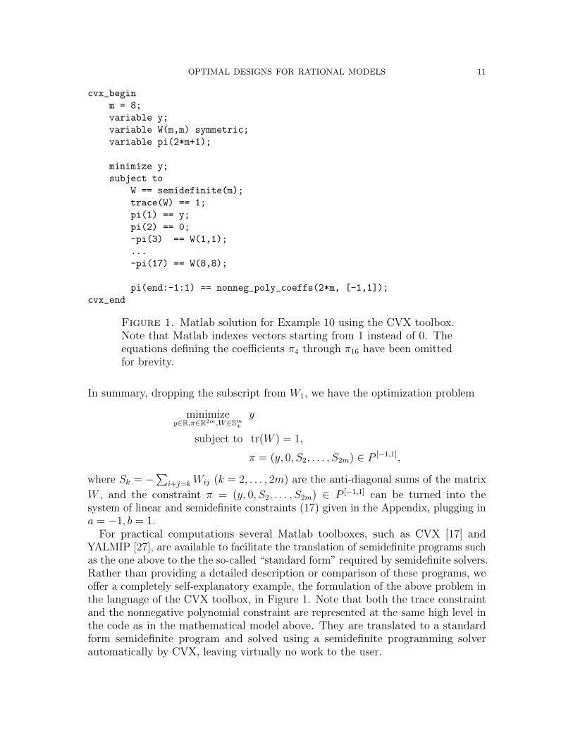
Figure 1. Matlab solution for Example 10 using the CVX toolbox.Note that Matlab indexes vectors starting from 1 instead of 0. Theequations defining the coefficients π4 through π16 have been omittedfor brevity.

In summary, dropping the subscript from W1, we have the optimization problem

minimizey∈R,π∈R2m,W∈Sm+

y

subject to tr(W ) = 1,

π = (y, 0, S2, . . . , S2m) ∈ P [−1,1],

where Sk = −∑

i+j=kWij (k = 2, . . . , 2m) are the anti-diagonal sums of the matrix

W , and the constraint π = (y, 0, S2, . . . , S2m) ∈ P [−1,1] can be turned into thesystem of linear and semidefinite constraints (17) given in the Appendix, plugging ina = −1, b = 1.

For practical computations several Matlab toolboxes, such as CVX [17] andYALMIP [27], are available to facilitate the translation of semidefinite programs suchas the one above to the the so-called “standard form” required by semidefinite solvers.Rather than providing a detailed description or comparison of these programs, weoffer a completely self-explanatory example, the formulation of the above problem inthe language of the CVX toolbox, in Figure 1. Note that both the trace constraintand the nonnegative polynomial constraint are represented at the same high level inthe code as in the mathematical model above. They are translated to a standardform semidefinite program and solved using a semidefinite programming solverautomatically by CVX, leaving virtually no work to the user.

12 DAVID PAPP

For example, solving the resulting problem for m = 8, the optimal vector π is the co-efficient vector of a degree 16 polynomial whose real roots are: {±1,±0.9207,±0.693,±0.3357}.It also has two imaginary roots. The eight real roots constitute the support of theE-optimal design. The same numerical example was considered in [5] with, of course,the same conclusion. The running time of SeDuMi in this example was 0.2 seconds.

Example 11 (A heteroscedastic polynomial model). Consider the cubic modelfi = ti−1, i = 1, . . . , 4, with heteroscedastic noise given by ω(t) = 1/(1 + t2), over thedesign space [−5, 5]. We chose this arbitrary model because it is one of the simplestamong those whose solution appears to not to be characterized.

The A-optimal design is computed as follows. The parameters Ai, Bi, Ci, Di in thesemidefinite representation (3) of A-optimality are determined first from Example 6.Using this representation, the constraints of the semidefinite programming problemin Theorem 9 are compiled in the following way.

• There are 4 semidefinite matrices W1, . . . ,W4 of order 5, and W5 is a nonneg-ative scalar.• The first constraint of (5b) is simply W5 = 1. The second constraint of (5b)

translates to (Wi)5,5 = 1 for each i = 1, . . . , 4.• We have deg(π) = 6, and comparing the coefficients on the two sides of (6),

we obtain a linear system of equations and matrix inequalities for (5c) and(5d), along the same lines as in the previous example.

The optimal solution is a polynomial whose real roots are {±5,±0.854}, this is thesupport of the A-optimal design.

In the remaining examples we shall refrain from the detailed list of the above steps,and concentrate on the main features of the models and the numerical results.

Example 12 (Polynomial models of high degree). We now consider the prob-lem of designing experiments for very high degree polynomial models in order to testthe numerical stability and scalability of our approach. Models involving high degreepolynomials are rarely justifiable, but they are good problems to test numericalstability, as they are notoriously ill-conditioned. For example, in the basic polynomialmodel, when fi = ti−1, i = 1, . . . , n, the the Fisher information matrix M(ξ) in (2)becomes a Hankel matrix, which is known to be ill-conditioned [38]. Also note thatin the case of rational models, the polynomial defined by (6) might also have a degreethat is considerably higher than the degree of the numerators and denominatorsof the functions fi, leading to potentially ill-conditioned optimization models. Thenumerical difficulties can be somewhat alleviated by using an orthogonal polynomialbasis in (1). In this example we look for the E-optimal polynomial design in theordinary polynomial regression model, but using the Legendre polynomial basis:fi = Pi−1, the (i − 1)-st Legendre polynomial defined by P0 = 1, P1(t) = t, andPn+1(t) = (n+ 1)Pn+1(t) + (2n+ 1)tPn(t)− nPn−1(t) for n ≥ 1.

The constraints are obtained along the same lines as in Example 10, except thatthe coefficients of π in (6) need to be changed as the moment matrix M(ξt) changeswith the change of basis.

OPTIMAL DESIGNS FOR RATIONAL MODELS 13

We solved the resulting semidefinite program for the degree 20 model; the compu-tation required 0.4 seconds. The optimal polynomial π is a nonnegative polynomialon [−1, 1] with single roots at the endpoints ±1, and double real roots at the points

{±0.981,±0.937,±0.872,±0.788,±0.686,±0.568,±0.438,±0.297,±0.150, 0}.

The E-optimal design is supported on these 21 points.

We remark that the use of high degree polynomials can also be circumvented usingpolynomial splines, which allow for the same large number of parameters withoutnumerical difficulties; this will the subject of a forthcoming paper.

Finally, we present an example using rational functions.

Example 13 (Measuring radiation parameters). Consider the measurementof total radiation emitted from point sources, whose intensity obeys the inversesquare law: Ii(r) = θir

−2 where Ii is the intensity of the radiation emitted by sourcei measured at distance r from the source, for some unknown parameter θi. Thelocations xi of the sources are known. The response variable in our model (1) isthe total radiation. To be estimated are the values θi, affected by parameters ofsources, shielding between the sources and detector, and several other factors. Inthis numerical example we consider a simple one-dimensional instance: the locationsof the three sources are x1 = −2, x2 = 2, x3 = 4, and we are interested in theeffective values of θi as measurable in the interval [−1, 1], where the variance of themeasurement error and the parameters are assumed to be constant.

The distance of a detector at t from the ith point source is ri = |t− xi|, so in ourmodel (1) we have fi = r−2

i = (t− xi)−2, i = 1, 2, 3, and I = [−1, 1]. The solution ofthe semidefinite program, which took 0.2 seconds, yielded a three-point support forthe E-optimal design: {−1, 0.231, 1}.

5. Reconstructing the optimal design

Once we obtained a non-zero polynomial π from the optimal solution of (19), wecan find the optimal design by solving a second semidefinite programming problem,using Theorem 8. But Theorem 9 is only useful if the polynomial π in the optimalsolution is not the zero polynomial. As the following example shows, in sufficientlydegenerate cases it might be.

Example 14. Consider the E-optimal design problem when m = 2, f(t) = (1, t)T,ω = 1, and I = [−1, 1]. Then the corresponding semidefinite programming problemsimplifies to

miny,W

y s.t. W < 0, tr(W ) = 1, π = (y −W11,−2W12,−W22) ∈ P [−1,1],

by essentially the same calculations as in Example 10. It is not hard to see that the setof optimal solutions to this problem is {(y,W ) | y = 1,W12 = 0,W11 +W22 = 1, 0 ≤W11 ≤ 1}. Hence, we have infinitely many solutions, including W11 = 1−W22 = 1,which corresponds to π(t) = 0. Choosing any other optimal solution yields apolynomial whose roots are the expected t = ±1.

14 DAVID PAPP

Alternatively, we can change f to a different basis of degree one polynomials. Thisdoes not really change the model, however, if we choose, for example, f(t) = (α, t)T

for any α > 1, the above problem disappears: the resulting semidefinite programmingproblem has a unique optimal solution, and that solution corresponds to a nonzeropolynomial π, with two real roots.

In the rest of the section we list a number of sufficient conditions that ensure thatthe optimal π in (5) is not the zero polynomial. The first one is perhaps the mostobvious one.

Lemma 15. Let f1, . . . , fm and ω in (1) be chosen such that 1 6∈ span{ωfifj | 1 ≤i ≤ j ≤ m}. Then no solution satisfying the constraints of (5) has π = 0.

Special cases covered by this lemma include designs for incomplete polynomialmodels with no intercept, such as those considered in [22] and [5], and modelsinvolving rational functions, such as Example 13 above.

The last observation of Example 14 also generalizes to E-optimal designs forarbitrary polynomial systems.

Lemma 16. Consider the E-optimal design problem for a polynomial model with atleast two parameters to be estimated. By choosing an appropriate basis {f1, . . . , fm}in (1) it can be guaranteed that no optimal solution of (5) has π = 0.

Proof. Let (y, W , π) be an optimal solution to (5). Then W = Y TY for some matrix

Y , and the polynomial q : t→ 〈W ,M(ξt)〉 can be written as q(t) = z(t)Tz(t) withz(t) = Y f(t). Consequently, q can only be a constant (and π can only be the zeropolynomial) if z(t) = Y f(t) is componentwise constant.

If 1 6∈ span{f1, . . . , fm}, then this is impossible, because Y = 0 is excluded by theconstraints (5b), which simplifies to tr(W ) = 1 for E-optimal designs.

If 1 ∈ span{f1, . . . , fm}, then we can assume without loss of generality that f1 = 1.

Now q can be a constant only if W11 = 1, and every other entry of W is zero, makingq(t) = 1 and y = 1. Replacing fi, i ≥ 2 by λfi with a sufficiently small positive λthat satisfies λ|fi(t)| < 1 for all t ∈ I ensures that this is not the optimal solution to(5). �

A similar argument applies to A-optimal designs for polynomial models. For brevitywe omit the details. As above, one can argue that by scaling the non-constant basisfunctions, solutions to the semidefinite programming problem that yield constantzero π cannot be optimal.

Lemma 17. Consider the A-optimal design problem for a polynomial model with atleast two parameters to be estimated. By choosing an appropriate basis {f1, . . . , fm}in (1) it can be guaranteed that no optimal solution of (5) has π = 0.

Finally, as a corollary to Theorem 9, we also obtain an upper bound on the sizeof the support set of the minimally-supported optimal designs.

Corollary 18. Let nω and dω be the degree of the numerator and denominator ofω, ni and di be the degree of the numerator and denominator of fi, and dden =

OPTIMAL DESIGNS FOR RATIONAL MODELS 15

lcm(dω, d21, . . . , d

2p). Furthermore, suppose that I is the union of k1 + k2 disjoint

closed intervals, k1 of which are singletons. (The remaining k2 intervals have distinctendpoints.) Then for every admissible criterion Φ for which the optimal solutionto (5) does not have π = 0 there is a Φ-optimal design supported on not more thanmin(1

2(k1+2k2+deg π), deg π) points, where deg π = dden+(nω−dω+2 maxi(ni−di))+.

Proof. We need to count the number of distinct zeros of the polynomial π in (5).On one hand, π cannot have more than deg π roots. On the other hand, since πis nonnegative over I, each of its zeros must be either an endpoint of an intervalconstituting I or a root of multiplicity at least two. Hence the number of distinctzeros of π is at most 1

2(k1 + 2k2 + deg π). Finally, the expression for deg π comes

directly from (6). �

6. Parameter subsystems, estimability

Often the experimenter is not interested in the entire parameter vector θ, butrather in a subset of them, or more generally in s ≤ m specific linear combinations ofthe parameters: kT

j θ, j = 1, . . . , s. Let K be the matrix whose columns are k1, . . . , ks;so far we have assumed s = m and K = I. An application of this more generalsetting is polynomial regression, when the experimenter needs to test whether thehighest degree terms in the model are indeed non-zero.

It can assumed without loss of generality that K has full (column) rank, and tomake the problem meaningful, it must be assumed that the parameters KTθ areestimable, that is,

range(K) ⊆ range(M), (7)

see for example [33, Chapter 3]. In this setting the matrix M is replaced by theinformation matrix (KTM †K)−1, where M † denotes the Moore–Penrose pseudo-

inverse of M . In particular, the optimal design is a probability measure ξ thatmaximizes the matrix (KTM †(ξ)K)−1, or the function ξ → Φ

((KTM †(ξ)K)−1

)for

some criterion function Φ compatible with the Lowner partial order.The optimization models for this setting can be developed analogously to the

model of the previous section. Since Φ is assumed to be compatible with the Lownerpartial order, maxM∈M Φ

((KTM †(ξ)K)−1

)is equivalent to

max{Φ(Y ) |M ∈ M , (KTM †K)−1 < Y < 0}. (8)

Note that the optimum does not change if we require Y to be positive definite, inwhich case the last two inequalities are equivalent to Y −1 < KTM †K. We shalluse now a Schur complement characterization of semidefinite matrices, which is ageneralization of the result used in Example 6.

Proposition 19 ([41, Theorem 1.20]). The symmetric block matrix(M KKT Z

)is posi-

tive semidefinite if and only if M < 0, Z < KTM †K, and range(K) ⊆ range(M).

By this proposition, (8) is equivalent to

max{Φ(Y ) |M ∈ M ,(M KKT Y −1

)< 0}.

16 DAVID PAPP

Using Schur complements again, the inversion from the last inequality can beeliminated, and we obtain the following equivalent optimization problem:

max{Φ(Y ) |M ∈ M , M < KYKT, Y < 0}. (9)

Finally, we can simplify this problem essentially identically to how we obtained(5) from (18). Doing so we obtain the following.

Theorem 20. Consider the linear model (1) and a matrix K ∈ Rm×s satisfyingrk(K) = s and the estimability condition (7). Then for every semidefinite repre-sentable criterion function Φ a polynomial π whose real zeros contain the supportof a Φ-optimal design for the parameter vector KTθ is an optimal solution of thefollowing semidefinite program:

minimizey∈R,V ∈Sm+ ,π∈Rd,

W1,...,Wp∈Sk+

y

subject to KTV K <p∑i=1

A∗i (Wi),

p∑i=1

〈Wi, Bi〉 = −1,

p∑i=1

C∗i (Wi) = 0,

π = Π(y, V,W1, . . . ,Wp) ∈ P I ,where Ai, Bi, Ci and Di come from Definition 3, and d is the degree of the polynomial

t→ lcm(den(ω), den(f 21 ), . . . , den(f 2

p ))

(y − 〈V,M(ξt)〉 −

p∑i=1

〈Wi, Di〉),

whose coefficient vector is denoted by Π(y, V,W1, . . . ,Wp).

We omit the rest of the proof as it is essentially identical to that of Theorem 9,given in the Appendix. The main difference is the appearance of the variable V ,which is the dual variable of the constraint M < KYKT.

7. Locally optimal designs for nonlinear models

In this section we show how to apply Theorems 9 and 20 to find locally optimaldesigns (with respect to various optimality criteria) for nonlinear rational models(see the definition and its motivation below). We consider the general nonlinearmodel

y(t) = f(t; θ) +N(0, σ(t)), t ∈ I, (10)

where f is a rational function of (t; θ), θ is an m-vector of unknown parameters. Thedesigns space I is the union of finitely many closed intervals, as before.

Nonlinear regression models are widely used and researched, but finding optimaldesigns for nonlinear regression is particularly challenging – so much so that evennumerical solutions to simple two- and three-variable models are highly non-trivialto obtain. (See for example [9] for recent results on a number of models used in

OPTIMAL DESIGNS FOR RATIONAL MODELS 17

dose-finding studies, and [26] for pharmacokinetic models.) Nonlinear rational models(where the response variable is a rational function of the explanatory variable andthe unknown parameters) and models involving exponential functions and logarithmsare particularly well studied. Imhof and Studden [24] considered E-optimal designsfor different classes of rational models. More recently, Dette et al. [10] investigatedE-optimal designs for a more general family of functions (not only rational functions),under the assumption that some partial derivatives of the model function form aweak Chebyshev system [25]. Note that this class of problems is not comparable tothe rational models we are considering: the partial derivatives of many non-rationalfunctions satisfy this criterion, but many rational models, for instance, the Emaxmodel from Example 21 below, are outside that class.

Perhaps the most fundamental complication in designing non-sequential exper-iments for nonlinear models is in the formulation of the problem as a meaningfuloptimization problem. For a nonlinear regression model (10) the Fisher informationmatrix corresponding to the design ξ is

M(ξ, θ) =

∫I(∂f(t, θ)/∂θ)(∂f(t, θ)/∂θ)Tω(t)dξ(t). (11)

It is immediate that (unlike in the linear case) the Fisher information matrix fornonlinear models depends on the parameters whose estimation is the purpose of theexperiments we are to design. Hence defining the optimal designs as the optimizersof the M(ξ, θ) is meaningless. Nevertheless, if the experimenter can guess reasonablevalues of the parameters, it can be useful to design the experiment that would beoptimal if the guessed parameters were correct. Some more advanced design methods,such as sequential designs [16] also build on the same concept, often called locallyoptimal designs. (The same ideas can also be used for the estimation of nonlinearfunctions of the parameters of a linear model.) Before considering the general case,let us look at a simple example that we shall readily generalize below.

Example 21. Consider the three-parameter Emax model

y(t) = θ0 +θ1t

t+ θ2

+N(0, 1), (12)

from the dose-finding study [9]. With the notation of (11),

∂f(t, θ)

∂θ=(1, t(t+ θ2)−1,−θ1t(t+ θ2)−2

)T,

so for every fixed value (θ∗0, θ∗1, θ∗2) of θ the integrand in the Fisher information matrix

(11) can be written as 1 t

t+θ∗2− θ∗1t

(t+θ∗2)2

tt+θ∗2

t2

(t+θ∗2)2− θ∗1t

2

(t+θ∗2)3

− θ∗1t

(t+θ∗2)2− θ∗1t

2

(t+θ∗2)3(θ∗1t)

2

(t+θ∗2)4

, (13)

18 DAVID PAPP

which is the same information matrix as the information matrix of the parametervector (α0, α1, α2) for the linear model

y(t) = α0 + α1t

t+ θ∗2+ α2

θ∗1t

(t+ θ∗2)2+N(0, 1). (14)

Hence, finding locally optimal designs for the Emax model (12) is equivalent to findingoptimal designs for the linear model (14), which is a linear model with rationalfunctions, hence Theorem 9 is applicable.

A further simplification is possible: we can find an equivalent polynomial model,and use Theorem 20 to find optimal designs. It is easy to verify that the matrix (13)can also be written as

KT

1 χ χ2

χ χ2 χ3

χ2 χ3 χ4

K

with χ = (t + θ∗2)−1 and K =

(1 1 00 −θ∗2 −θ∗10 0 θ∗1θ

∗2

). Hence, for every fixed θ∗ the Fisher

information matrix of the design ξ for model (12) is identical to the Fisher informationmatrix of the design that puts ξ(ti) mass to the point χi = (ti + θ∗2)−1 for the three-parameter linear model

y(χ) = α0 + α1χ+ α2χ2 +N(0, 1) (15)

and the parameter vector KTα = (α0, α0 − α1θ∗2, α2θ

∗1θ∗2 − α1θ

∗1)T. Now the problem

is reduced to polynomial regression, and Theorem 20 is applicable.

Generally, for a nonlinear regression model (10) with m parameters, the problemof finding a locally optimal design for a given parameter vector θ∗ is equivalentto finding the optimal design for the associated linear model of the form (1) withfi = (∂f)/(∂θi)

∣∣θ=θ∗

, i = 1, . . . ,m. If f is a rational function of (t, θ), then so are itspartial derivatives. Hence the equivalent linear model (for every fixed value of θ) isalways one with rational functions fi.

The same observation was used in [10] to derive E-optimal designs for the class ofnonlinear regression models where the partial derivatives form a weak Chebyshevsystem. Now this assumption can be dropped, and other optimality criteria can alsobe considered.

8. Optimal designs in other functional spaces

Most of Section 3 applies to every fi and ω, not only to rational functions; forexample, (22) is not specific to polynomials or rational functions. As long as the setof constraints (23) can be expressed by finitely many semidefinite constraints (or inany other computationally tractable manner), the same approach works. Examplesinclude the following (we consider only the homoscedastic case for simplicity):

(1) fi(t) = cos(it) for every i ∈ N and t;(2) f2i(t) = cos(it), f2i+1(t) = sin(it) for every i ∈ N, and t;(3) fi(t) = exp(it) for every i ∈ N and t.

OPTIMAL DESIGNS FOR RATIONAL MODELS 19

These three examples, however, do not truly generalize the approach of Section 3,since they can also be reduced to the polynomial case by an appropriate change ofvariables. (We omit the details.)

Our estimate on the number of support points is also valid for some functionalspaces other than polynomials. The only property of polynomials that we used werethat their degree bounds the number of their roots (counted with multiplicity: rootsin the interior of the domain have multiplicity two). Hence, bounds similar to theone in Corollary 18 can be obtained for models where the functions {ωfifj|i, j} forma Chebyshev system.

9. Discussion

Computing optimal designs for linear models involving rational functions is easywhen the design space is finite, hence the key difficulty in obtaining optimal designsfor infinite design spaces, such as intervals or unions of intervals, is that the finitesupport of an optimal design has to be determined. Symbolic or closed form solutionsare unavailable for most models, and their scope is often limited by assumptionsthat are neither technical, nor have any statistical interpretation. In this paper, wehave presented a method that does not rely on such assumptions. It is an effectivemethod to determine a polynomial whose zeros contain the support of the optimaldesigns. The method is applicable to every linear regression problem involving onlyrational functions; it treats D-, A-, E-, and general Φp optimal designs in a unifiedmanner, and generalizes to the heteroscedastic case if the variance of the noise isa positive rational function. The design space can be an interval or the union offinitely many intervals.

This level of generality is far greater than what appears to be possible by closed-formapproaches. It is achieved at the price of providing numerical, rather than symbolic,solutions: the method generates the (numerical) coefficients of the sought polynomial.The main step of the method is the solution of a semidefinite programming problem,which can be done (to high precision) with readily available software in trivial runningtime. Unlike other iterative methods previously proposed in the literature, includingall of those based on coordinate descent, semidefinite programming algorithms havea theoretically guaranteed low running time, and are guaranteed to find the globallyoptimal design, rather than a local optimum. This is of considerable practicalimportance, with the potential for instance to impact design software development.

Further study of the optimality conditions of the main optimization model mightalso yield new theoretical insights.

Through a number of examples we have demonstrated the flexibility of the proposedmethod, and we also found that the algorithm is robust enough to handle ill-conditioned problems involving high-degree polynomials, and yields solutions in afraction of a second for problems of practical size.

A corollary of our main theorem is a bound on the size of the support set, and ananalogous optimization model for the estimation of parameter subsystems.

20 DAVID PAPP

Most results of this paper readily generalize to linear models involving certainexponential families rather than rational functions; these include Fourier regression,where the model is a trigonometric polynomial with unknown coefficients. Themethod may also be used to find locally optimal designs for nonlinear models. Inthis area almost no symbolic solutions are available, but model-specific numericalmethods are abound. Details are available from the author, and may be subject of afuture paper.

A few important questions remain open. The first one is how to extend theresults of Section 5. Since the optimal solution to the problem (5) is sensitive toboth the representation of the optimality criterion Φ and also to the basis {fi}of the space of regression functions (meaning that equivalent representations ofΦ and basis transformations lead to different optimal solutions), one may readilyconjecture that for every model (1) and for every admissible optimality criterion onecan find an equivalent model (that is, a basis {fi} of the same functional space) anda semidefinite representation (3) for Φ such that the optimal π in every solution of(5) is nonzero.

Another subject of future research may be the generalization of our results tolarger classes of functions. Chebyshev systems are natural candidates to look at,but more importantly, the ideas of the paper would generalize word by word toevery family (f1, . . . , fm) and weight function ω for which functions in the spacespan{ωfifj|i, j} are easy to maximize. Hence, identifying such spaces of functionswould be particularly important.

Finally, the ability to design experiments in a discontinuous design space isextremely relevant in practice, especially in the multivariate case (e.g., when mea-surements cannot be taken at inaccessible locations, or are practically impossiblevery close to signal sources). Existing models with closed-form solutions are notapplicable, and most of the current numerical methods cannot address this problemeven in the univariate case, aside from sporadic results involving two disjoint intervalsfor a few concrete models.

The applicability of the proposed method in the multivariate setting also requiresfurther study.

References

1. The optimum experimental design website, http://www.optimal-design.org/, Accessed onApril 1, 2011.

2. Ali Babapour Atashgah and Abbas Seifi, Optimal design of multi-response experiments usingsemi-definite programming, Optimization in Engineering 10 (2009), no. 1, 75–90.

3. Aharon Ben-Tal and Arkadi Nemirovski, Lectures on modern convex optimization, SIAM,Philadelphia, PA, 2001.

4. Stephen P. Boyd and Lieven Vandenberghe, Convex optimization, Cambridge University Press,2004.

5. Fu-Chuen Chang and Berthold Heiligers, E-optimal designs for polynomial regression withoutintercept, Journal of Statistical Planning and Inference 55 (1996), no. 3, 371–387.

OPTIMAL DESIGNS FOR RATIONAL MODELS 21

6. Fu-Chuen Chang and Hung-Ming Lin, On minimally-supported D-optimal designs for polynomialregression with log-concave weight function, Metrika 65 (2007), no. 2, 227–233.

7. A. de la Garza, Spacing of information in polynomial regression, Annals of MathematicalStatistics 25 (1954), no. 1, 123–130.

8. Holger Dette, Optimal designs for a class of polynomials of odd or even degree, The Annals ofStatistics 20 (1992), no. 1, 238–259.

9. Holger Dette, Frank Bretz, Andrey Pepelyshev, and Jose Pinheiro, Optimal designs for dose-finding studies, Journal of the American Statistical Association 103 (2008), no. 483, 1225–1237.

10. Holger Dette, Viatcheslav B. Melas, and Andrey Pepelyshev, Optimal designs for a class ofnonlinear regression models, The Annals of Statistics 32 (2004), no. 5, 2142–2167.

11. Holger Dette and Ingo Roder, Optimal product designs for multivariate regression with missingterms, Scandinavian Journal of Statistics 23 (1996), no. 2, 195–208.

12. Holger Dette and William J. Studden, The theory of canonical moments with applications instatistics, probability, and analysis, Wiley Interscience, New York, NY, September 1997.

13. Zhide Fang, D-optimal designs for polynomial regression models through origin, Statistics &Probability Letters 57 (2002), no. 4, 343–351.

14. V. V. Fedorov, Theory of optimal experiments, Academic Press, New York, NY, 1972.15. Lenka Filova and Maria Trnovska, Computing maximin efficient designs using the methods of

semidefinite programming, Tech. report, Comenius University, Bratislava, Slovakia, May 2010.16. I. Ford and S. D. Silvey, A sequentially constructed design for estimating a nonlinear parametric

function, Biometrika 67 (1980), no. 2, 381–388.17. Michael Grant and Stephen Boyd, CVX: Matlab software for disciplined convex programming

(web page and software), Stanford University, December 2007, http://cvxr.com/cvx/.18. P. G. Guest, The spacing of observations in polynomial regression, The Annals of Mathematical

Statistics 29 (1958), no. 1, 294–299.19. Emilie V. Haynsworth, Determination of the inertia of a partitioned Hermitian matrix, Linear

Algebra and its Applications 1 (1968), no. 1, 73–81.20. Didier Henrion and Jean-Bernard Lasserre, GloptiPoly: Global optimization over polynomials

with Matlab and SeDuMi, ACM Transactions on Mathematical Software 29 (2002), 165–194.21. Paul G. Hoel, Efficiency problems in polynomial estimation, The Annals of Mathematical

Statistics 29 (1958), no. 4, 1134–1145.22. Mong-Na Lo Huang, Fu-Chuen Chang, and Weng Kee Wong, D-optimal designs for polynomial

regression without an intercept, Statistica Sinica 5 (1995), no. 2, 441–458.23. Lorens A. Imhof, O. Krafft, and M. Schaefer, D-optimal designs for polynomial regression with

weight function x/(1+x), Statistica Sinica 8 (1998), no. 4, 1271–1274.24. Lorens A. Imhof and William J. Studden, E-optimal designs for rational models, The Annals of

Statistics 29 (2001), no. 3, 763–783.25. Samuel Karlin and William J. Studden, Tchebycheff systems, with applications in analysis and

statistics, Pure and Applied Mathematics, vol. XV, Wiley Interscience, New York, NY, 1966.26. Gang Li and Dibyen Majumdar, Some results on D-optimal designs for nonlinear models with

applications, Biometrika 96 (2009), no. 2, 487–493.27. Johan Lofberg, YALMIP: A toolbox for modeling and optimization in MATLAB, Proceedings

of the CACSD Conference (Taipei, Taiwan), 2004.28. Franz Lukacs, Verscharfung der ersten Mittelwersatzes der Integralrechnung fur ra-

tionale Polynome, Mathematische Zeitschrift 2 (1918), 229–305, Available fromhttp://www.digizeitschriften.de/.

29. Ruth K. Meyer and Christopher J. Nachtsheim, The coordinate-exchange algorithm for con-structing exact optimal experimental designs, Technometrics 37 (1995), no. 1, 60–69.

22 DAVID PAPP

30. Yurii Nesterov, Squared functional systems and optimization problems, High PerformanceOptimization (H. Frenk, K. Roos, T. Terlaky, and S. Zhang, eds.), Appl. Optim., Kluwer Acad.Publ., Dordrecht, 2000, pp. 405–440.

31. Jorge Nocedal and Stephen J. Wright, Numerical optimization, 2 ed., Springer, New York, NY,2000.

32. Victor Y. Pan, Structured matrices and polynomials: unified superfast algorithms, Birkhauser,Boston, MA, 2001.

33. Friedrich Pukelsheim, Optimal design of experiments, Wiley Interscience, 1993.34. Ralph Tyrrell Rockafellar, Convex analysis, Princeton University Press, Princeton, NJ, 1970.35. Andrzej Ruszczynski, Nonlinear optimization, Princeton University Press, Princeton, NJ, 2005.36. Stephen M. Stigler, Optimal experimental design for polynomial regression, Journal of the

American Statistical Association 66 (1971), no. 334, 311–318.37. Jos F. Sturm, Using SeDuMi 1.02, a Matlab toolbox for optimization over symmetric cones,

Optimization Methods and Software 11–12 (1999), no. 1–4, 625–653.38. Evgenij E. Tyrtyshnikov, How bad are Hankel matrices?, Numerische Mathematik 67 (1994),

no. 2, 261–269.39. Lieven Vandenberghe and Stephen P. Boyd, Semidefinite programming, SIAM Review 38 (1996),

no. 1, 49–95.40. Henry Wolkowicz, Romesh Saigal, and Lieven Vandenberghe (eds.), Handbook of semidefinite

programming: Theory, algorithms, and applications, Kluwer, Norwell, MA, 2000.41. Fuzhen Zhang (ed.), The Schur complement and its applications, Springer, New York, NY,

2005.

Appendix A. The semidefinite representability of polynomials overintervals

For a ∆ ⊆ R let P∆n denote the set of degree n polynomials nonnegative over ∆.

The following representation of nonnegative polynomials is well-known:

Proposition 22 ([28]). For every polynomial p of degree n, p ∈ P [a,b]n if and only if

p(t) =

{r2(t) + (t− a)(b− t)q2(t) (if n = 2k)

(t− a)r2(t) + (b− t)s2(t) (if n = 2k + 1)

for some polynomials r and s of degree k and q of degree k − 1.

On the other hand, functions expressible as sums of squares of functions from agiven finite dimensional functional space (such as polynomials of a fixed degree) aresemidefinite representable; see [30] for a constructive proof of this claim. Applyingthis construction to part (2) of Proposition 22 yields the following.

Proposition 23 ([30]). Suppose p is a polynomial of degree n = 2m + 1, p(t) =∑nk=0 pkt

k, and let a < b are real numbers. Then p ∈ P [a,b]n if and only if there exist

positive semidefinite matrices X = (xij)mi,j=0 and Y = (yij)

mi,j=0 satisfying

pk =∑i+j=k

(−axij + byij) +∑

i+j=k−1

(xij − yij) (16)

for all k = 0, . . . , 2m+ 1.

OPTIMAL DESIGNS FOR RATIONAL MODELS 23

Similarly, if p is a polynomial of degree n = 2m, then p ∈ P [a,b]n if and only if there

exist positive semidefinite matrices X = (xij)mi,j=0 and Y = (yij)

m−1i,j=0 satisfying

pk =∑i+j=k

(xij − abyij) +∑

i+j=k−1

(a+ b)yij −∑

i+j=k−2

yij (17)

for all k = 0, . . . , 2m.

This is rather involved (and the details are only important for the purposes ofactual computations), but close inspection reveals that this proposition characterizes

P [a,b]n as a linear image of the Cartesian product of two semidefinite cones, thus, it

proves the semidefinite representability of P [a,b]n in the sense of Definition 1.

Since the intersection of semidefinite representable sets are also semidefiniterepresentable, it follows that PIn is semidefinite representable for every union offinitely many closed intervals I.

Appendix B. Proof of Theorem 9

Consider the problem of finding max{Φ(M(ξ)) | ξ ∈ Ξ(I)}, where Ξ(I) is the setof probability measures on I with finite support, and M is the Fisher informationmatrix defined by (2). Considering the Fisher information as the variable, this canbe expressed as a finite dimensional optimization problem:

max{Φ(M) |M ∈ M }, where M = {M(ξ) | ξ ∈ Ξ(I)}. (18)

Let ξt be the probability measure that assigns all of its mass to t ∈ I. Because Iis assumed to be compact and the mapping t→M(ξt) is continuous, {M(ξt) | t ∈ I}is compact. Hence, M = conv{M(ξt) | t ∈ I} is a convex compact set, and theoptimization problem (18) is well-defined: The maximum is finite, and is attained(for every continuous function Φ).

Now let us assume that Φ is semidefinite representable. Then using the notationsof Definition 3, problem (18) may be written as follows.

maximizez∈R, u∈Rl,M∈M

z

subject to Ai(M) +Biz + Ci(u) +Di < 0, i = 1, . . . , p,(19)

where Ai, Bi, Ci, and Di are the functions and matrices as in Definition 3.Because Sk+ is a closed convex cone, (19) is equivalent to the following Lagrangian

relaxation (in which the dual variable Wi is the Lagrange multiplier associated withthe ith constraint):

maxz,u,M∈M

infWi<0

(i=1,...,p)

z +

p∑i=1

〈Wi, Ai(M) +Biz + Ci(u) +Di〉 (20)

Suppose that Φ is admissible with respect to M . Then the optimization problem(19) has a Slater point, consequently its optimum is equal to optimum of its dualproblem [35, Chapter 4], obtained by replacing the “max inf” by “min sup” in the

24 DAVID PAPP

Lagrangian (20). This dual problem then can be simplified as follows (C∗i denotesthe dual operator of Ci):

minW1,...,Wp<0

supz,u,M∈M

z +

p∑i=1

〈Wi, Ai(M) +Biz + Ci(u) +Di〉

= minW1,...,Wp<0

supz,u,M∈M

z

(1 +

p∑i=1

〈Wi, Bi〉

)+

+

p∑i=1

〈C∗i (Wi), u〉+

p∑i=1

〈Wi, Ai(M) +Di〉

= minW1,...,Wp<0∑i〈Wi,Bi〉=−1∑i C

∗i (Wi)=0

supM∈M

p∑i=1

〈Wi, Ai(M) +Di〉 (21)

= minW1,...,Wp<0∑i〈Wi,Bi〉=−1∑i C

∗i (Wi)=0

maxM∈M

p∑i=1

〈Wi, Ai(M) +Di〉.

(The last equation simply means that the supremum is attained.)Finally, with the help of a dummy variable y the optimization problem in the last

line can be conveniently written as:

minimizey∈R,

W1,...,Wp∈Sk

y

subject to Wi < 0 i = 1, . . . , p,p∑i=1

〈Wi, Bi〉 = −1,

p∑i=1

C∗i (Wi) = 0,

y ≥p∑i=1

〈Wi, Ai(M) +Di〉 ∀M ∈ M .

(22)

Aside from the last set of constraints, which is an uncountably infinite collectionof linear inequalities, every constraint is either a linear equality or a linear matrixinequality on the variables Wi. Using that M = conv{M(ξt) | t ∈ I}, the last set ofconstraints can also be simplified to

y −p∑i=1

〈Wi, Ai(M(ξt)) +Di〉 ≥ 0 ∀ t ∈ I. (23)

Since M(ξt) is a matrix whose entries are rational functions of t, this inequalityexpresses the nonnegativity of a rational function (over I) that lives in the space

V = span ({ωfifj | i, j = 1, . . . ,m} ∪ {1}) ,

OPTIMAL DESIGNS FOR RATIONAL MODELS 25

with variable coefficients. Multiplying both sides with the least common denominatorof the functions ωfifj (which is positive on I) turns (23) to the equivalent inequality(5d) with Π defined in (6), giving us (5).

Finally, suppose (y, π, W1, . . . , Wp) is an optimal solution to (5). Then, since (5),

(21), and (22) are equivalent, (y, W1, . . . , Wp) is also an optimal solution to (22),

and because the optimum in (21) is attained, there exists an M ∈ M that satisfiesthe last constraint of (22) with inequality. The way we obtained (22) from (18)

ensures that this M is also an optimal solution to our original problem (18). Suppose

M = M(ξ) for some measure ξ ∈ Ξ(I) that is concentrated on {t1, . . . , tk} ⊆ I and

assigns weight λi to ti, i = 1, . . . , k. Then with the optimal y and W1, . . . Wp each ofthese ti must satisfy (23) with equality. Consequently each ti is a root of π. �

David Papp, Northwestern University, Department of Industrial Engineering andManagement Sciences, Technological Institute, 2145 Sheridan Rd, C210, Evanston,IL 60208. Email: dpapp@iems.northwestern.edu