HAL Id: halshs-00323581https://halshs.archives-ouvertes.fr/halshs-00323581

Submitted on 22 Sep 2008

HAL is a multi-disciplinary open accessarchive for the deposit and dissemination of sci-entific research documents, whether they are pub-lished or not. The documents may come fromteaching and research institutions in France orabroad, or from public or private research centers.

L’archive ouverte pluridisciplinaire HAL, estdestinée au dépôt et à la diffusion de documentsscientifiques de niveau recherche, publiés ou non,émanant des établissements d’enseignement et derecherche français ou étrangers, des laboratoirespublics ou privés.

Optimal household energy management and economicanalysis: from sizing to operation scheduling

T.T. Ha Pham, Cédric Clastres, F. Wurtz, S. Bacha, Éric Zamaï

To cite this version:T.T. Ha Pham, Cédric Clastres, F. Wurtz, S. Bacha, Éric Zamaï. Optimal household energy man-agement and economic analysis: from sizing to operation scheduling. Advances and Applicationsin Mechanical Engineering and Technology, Scientific Advances Publishers, 2010, 1 (1), pp.35-68.�halshs-00323581�

LABORATOIRE D’ECONOMIE DE LA PRODUCTION ET DE L’INTEGRATION INTERNATIONALE

UMR 5252 CNRS - UPMF

______________________

LEPII BP 47 - 38040 Grenoble CEDEX 9 - France

1221 rue des Résidences - 38400 Saint Martin d'Hères Tél.: + 33 (0)4 76 82 56 92 - Télécopie : + 33 (0)4 56 52 85 71

lepii@upmf-grenoble.fr - http://www.upmf-grenoble.fr/lepii

_____________________

CAHIER DE RECHERCHE

N° 11

Optimal household energy management and economic analysis : from sizing to operation scheduling

T.T. Ha Pham1

C. Clastres1,2

F. Wurtz1

S. Bacha1

E. Zamaï3

juillet 2008

1 Grenoble Electrical Engineering (G2ELAB) - INPG, UJF, CNRS 2 LEPII – UPMF, CNRS 3 Laboratoire des sciences pour la conception, l'optimisation et la production (G-SCOP) - INPG, UJF, CNRS

1

Optimal household energy management and economic

analysis: from sizing to operation scheduling

T.T. Ha Pham1, C. Clastres

1,2,*, F. Wurtz

1, S. Bacha

1, E. Zamaï

3

1 Grenoble Electrical Engineering (G2ELAB) CNRS - INPG / UJF

BP 46-38402 Saint Martin d'Heres, France

2 LEPII-EREN - University of Grenoble II BP 47 - 38040 Grenoble Cedex 9 - France

3 Laboratoire des sciences pour la conception, l'optimisation et la production (G-SCOP) CNRS - INPG / UJF

46, avenue Félix Viallet - 38031 Grenoble, France

July 2008

Abstract

The study presented in this paper takes part in a project aiming to increase the value of solar production for

residential application with a medium-term vision where preferential solar energy subsidies will decrease

before to disappear. This study is dedicated to propose and develop optimal energy architecture at supply

side, a multi-source system based on photovoltaic (PV) solar energy connecting to main electrical network,

taking further into account the effectiveness of intelligent demand side management. To investigate this issue,

a method of optimal supplying system sizing and household energy management has been developed. This

method, which has been formulated employing Mix Integer Linear Programming (MILP), enables the

calculation of the appropriate configuration for power supply system and the optimal operation control to be

applied. Using a Net Present Value (NPV) and Probability Index (P.I) basis, the economic analysis allows

estimation of the viability of the proposed system under different factors of influence such as renewable

energy policies, technology evolutions leading to cheaper installed PV module cost and deregulated

electricity market. Simulation results show that, the solution makes it possible for PV power to be

significantly valued by the customers without subsidized measures.

Keywords: connected-grid PV system, battery storage, sizing optimization, energy management, MILP

* Corresponding author

Tel. : +33 (0)476826430; Fax : +33 (0)476826300

E-mail address : cedric.clastres@g2elab.inpg.fr

This work was supported by the French National Research Agency - PV Program and is included in the MULTISOL

Project.

2

Nomenclature

Model parameters

ηB Battery storage efficiency

CB Coefficient cost of storage system, [€/kWh]

cg(t) Grid energy price, [€/kW]

cgn Coefficient of grid connection fix cost, [€/kW]

Cond Coefficient cost of inverter, [€/kW]

CPV Coefficient cost of peak power rate of PV module, [€/kWp]

cs(t) Sellback price of local production, [€/kWh]

i Discount rate, [%/year]

k Study year, [year]

rch Charge coefficient rate, [kW/h]

rdch Discharge coefficient rate, [kW/h]

SP(t) Spot price, [€/kWh]

t Calculation step time, [hour]

T Study period, equal to lifetime of installation, [year]

Decision variables

α(t) Decision binary variable, α(t) = 1 if the battery is in the charging mode, α(t) = 0 if the battery

in the discharging mode

β(t) Decision binary variable, β(t) = 1 if the system imports grid energy, β(t) = 0 if the system

purchases its PV production

ω(t) Decision variable, used to translate the absolute relation into linear representation

Pbin(t) Charge power consign [kW]

Pbout(t) Disharge power consign [kW]

Pg(t) Consumed grid power [kW]

PL(t) Electrical demand prevision [kW]

PLP(t) Consumed power by controllable loads

PNLP(t) Consumed power by non-controllable loads

PPV(t) PV available power [kW]

Ps(t) PV power to be used locally [kW]

SOC(t) Temporal state of charge [kWh]

z(t) PV power to be injected to network [kW]

1. Introduction

In Europe, the rapid growth connected-grid PV systems in the residential sector over the last year have

been promoted by government supported programs with considerable investment subsidies [1]. By this way,

the PV power producers find it currently beneficial to sellback maximum of his solar production to electricity

utilities. This is especially convenient for short-time frame when PV penetration rate in electrical network still

3

remains marginal or to be applied in the small scale applications.

However, actual policies to develop the use of renewable energies would evolve. Feed-in tariffs could be

lower to lessen the cost of renewable energies promotion. They would be then disappeared (as in Japan, for

example) or replaced by another system less attractive (green certificates or market component as in Spain

[2]). Given that context, it will be difficult to justify the real interest of this operation mode of PV connected-

grid system as currently.

However, the potential benefits of PV system are quite large. The core idea is that PV applications could

impact both supply-side and demand-side issues. Aside being an alternative for the housing power supply

having lower environment impacts, PV also serve as a vehicle for triggering efficient energy utilization by

influencing consumer awareness of energy saving.

Another observation and analysis of energy markets changing also make connected-grid PV system

interesting to study. The liberalization process leads to the end of regulated tariffs (toward 2011 in France).

So, market price contracts would be generalized to all consumers, with certainly an indexation on volatile

spot prices. A consumer could have incentives and benefits to develop PV generation to limit the price risk

volatility. This is, for a household consumer, a mean to hedge it against high prices.

Lastly, energy vulnerability of several European countries and climate change policies imply to develop

cleaner production and demand-side management (rationale use of energy, energy positive houses as in Great-

Britain where all new houses in 2016 would be zero Greenhouse Gas emission [3]).

These issues at stake ask for investigating the innovative energy architecture for housing applications. It is

expected that the building of tomorrow should be a positive, green and intelligent element. The project

sustaining this paper, MULTISOL, has the ambition to design an economical and technical efficient

framework for household energy management. A new architecture is proposed with: at supply side, a PV-

based multi-source system; and at demand side, source and load co-management.

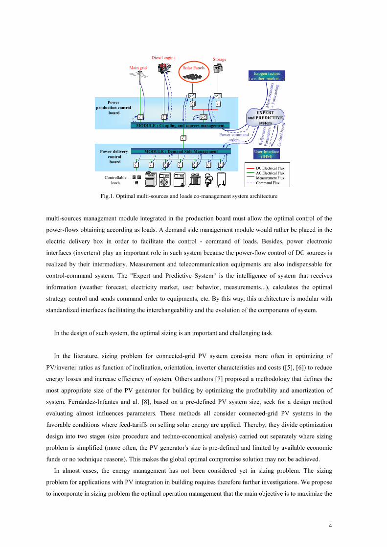
2. Model framework description

In this project, the works to design and demonstrate the multi-sources and loads co-management system

architecture has been in progress. We suggest separating the components between the house and electric

network into two connection boards (Fig. 1), [4]. All production means such as PV generator, battery,

network, and possible diesel or others complementary sources, are connected in the "Power production

control board" to supply loads via the traditional electric delivery box called "Power delivery control board".

A coupling and

∗ STC is specified at condition air mass of 1.5, radiation of 1 kW/m2, and ambient temperature of 25°C.

4

Solar Panels

StorageDiesel engine

Main grid

= ~= ~

==

==

==

==

Controllable

loads

Power

production control

board

Power delivery

control

board

DC Electrical Flux

AC Electrical Flux

Measurement Flux

Command Flux

DC Electrical Flux

AC Electrical Flux

Measurement Flux

Command Flux

EXPERT

and PREDICTIVE

system

EXPERT

and PREDICTIVE

system

Measurements

+ Forecasting

Exogen factors

(weather, market…)

User Interface

(IHM)

Control board

References

Param

eters

Power command

orders

MODULE ; Coupling and sources management

MODULE : Demand Side Management

Fig.1. Optimal multi-sources and loads co-management system architecture

multi-sources management module integrated in the production board must allow the optimal control of the

power-flows obtaining according as loads. A demand side management module would rather be placed in the

electric delivery box in order to facilitate the control - command of loads. Besides, power electronic

interfaces (inverters) play an important role in such system because the power-flow control of DC sources is

realized by their intermediary. Measurement and telecommunication equipments are also indispensable for

control-command system. The "Expert and Predictive System" is the intelligence of system that receives

information (weather forecast, electricity market, user behavior, measurements...), calculates the optimal

strategy control and sends command order to equipments, etc. By this way, this architecture is modular with

standardized interfaces facilitating the interchangeability and the evolution of the components of system.

In the design of such system, the optimal sizing is an important and challenging task

In the literature, sizing problem for connected-grid PV system consists more often in optimizing of

PV/inverter ratios as function of inclination, orientation, inverter characteristics and costs ([5], [6]) to reduce

energy losses and increase efficiency of system. Others authors [7] proposed a methodology that defines the

most appropriate size of the PV generator for building by optimizing the profitability and amortization of

system. Fernández-Infantes and al. [8], based on a pre-defined PV system size, seek for a design method

evaluating almost influences parameters. These methods all consider connected-grid PV systems in the

favorable conditions where feed-tariffs on selling solar energy are applied. Thereby, they divide optimization

design into two stages (size procedure and techno-economical analysis) carried out separately where sizing

problem is simplified (more often, the PV generator's size is pre-defined and limited by available economic

funds or no technique reasons). This makes the global optimal compromise solution may not be achieved.

In almost cases, the energy management has not been considered yet in sizing problem. The sizing

problem for applications with PV integration in building requires therefore further investigations. We propose

to incorporate in sizing problem the optimal operation management that the main objective is to maximize the

5

benefit for system's owner. A result analysis method is also given. Once built up, this method will provide a

tool for user to automatically dimension his installation and analyze the economic viability of system under

different conditions.

3. Mathematical problem formulation

Sizing optimization problems presented herein are formulated using a Mix Integer Linear Programming

(MILP) algorithm which requires all mathematical representations (objective function and constraints)

expressed in standard form, [9]:

Minimize )(xf

Subject to: Ax ≤ b

Aeq.x = beq

lb ≤ x ≤ ub

With: x are the variables (continue, binary or integers)

A, Aeq are matrixes

f, b, beq are vectors

The x vector (unknown variables) includes:

- sizing variables : peak power of PV array (PPVp), battery storage capacity (Smax), grid connection

contracted rate power (Pgmax)

- hourly operation variables: charging power set-point Pbin(t), discharging power set-pointPbout(t),

consumed grid power Pg(t), surplus power z(t), consumed controllable load PLP(t), and consumed

non-controllable load PNLP(t)

- decision binary variables: α(t) used to distingue charging and discharging mode in battery

operation model, β(t) used to define the mode for exchanging energy with the network.

Each variable is limited to its lower (lb) and upper (ub) bounds. A, b, Aeq, beq represent the inequality and

equality equation constraints of x. f is the vector of objective function.

The following flowchart shows the mains steps of optimization algorithm:

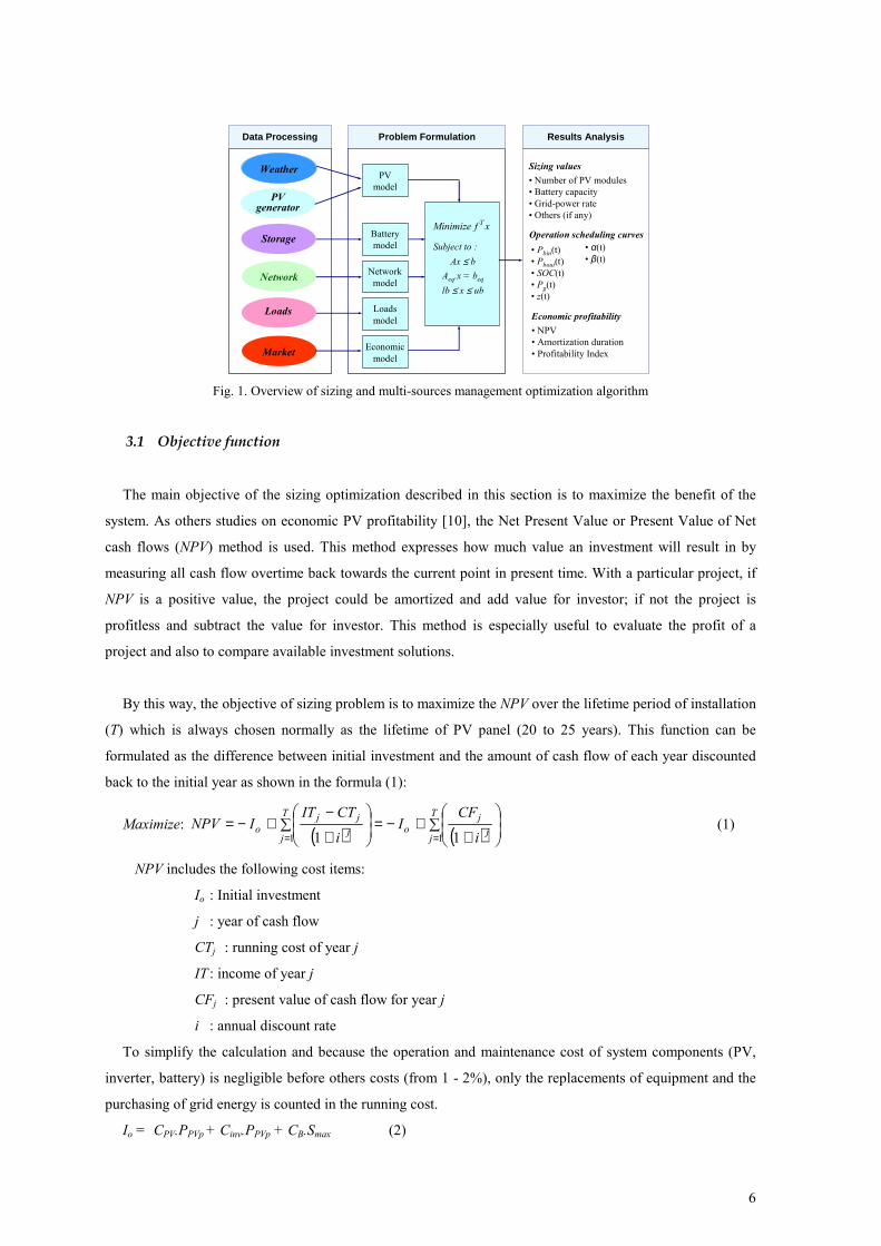
6

PV generator

Storage

Network

Weather

Market

Loads

Battery

model

PV

model

Network

model

Loads

model

Economic

model

xfMinimize T

Subject to :

Ax ≤ b

Aeq.x = beq

lb ≤ x ≤ ub

Data Processing Problem Formulation Results Analysis

Sizing values

• Number of PV modules

• Battery capacity

• Grid-power rate

• Others (if any)

Operation scheduling curves

• Pbin(t)

• Pbout(t)

• SOC(t)

• Pg(t)

• z(t)

• α(t)

• β(t)

Economic profitability

• NPV

• Amortization duration

• Profitability Index

Fig. 1. Overview of sizing and multi-sources management optimization algorithm

3.1 Objective function

The main objective of the sizing optimization described in this section is to maximize the benefit of the

system. As others studies on economic PV profitability [10], the Net Present Value or Present Value of Net

cash flows (NPV) method is used. This method expresses how much value an investment will result in by

measuring all cash flow overtime back towards the current point in present time. With a particular project, if

NPV is a positive value, the project could be amortized and add value for investor; if not the project is

profitless and subtract the value for investor. This method is especially useful to evaluate the profit of a

project and also to compare available investment solutions.

By this way, the objective of sizing problem is to maximize the NPV over the lifetime period of installation

(T) which is always chosen normally as the lifetime of PV panel (20 to 25 years). This function can be

formulated as the difference between initial investment and the amount of cash flow of each year discounted

back to the initial year as shown in the formula (1):

Maximize: ( ) ( )∑

++−=∑

+

−+−=

==

T

jj

jo

T

jj

jjo

i

CFI

i

CTITINPV

11 11 (1)

NPV includes the following cost items:

Io : Initial investment

j : year of cash flow

CTj : running cost of year j

IT : income of year j

CFj : present value of cash flow for year j

i : annual discount rate

To simplify the calculation and because the operation and maintenance cost of system components (PV,

inverter, battery) is negligible before others costs (from 1 - 2%), only the replacements of equipment and the

purchasing of grid energy is counted in the running cost.

Io = CPV.PPVp + Cinv.PPVp + CB.Smax (2)

7

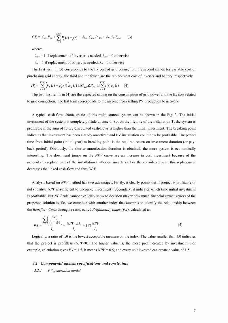
CTj = Cgn.Pgn +∑=

8760

1

)().(t

gg tctP + λinv .Cinv.PPVp + λB.CB.Smax (3)

where:

λinv = 1 if replacement of inverter is needed, λinv = 0 otherwise

λB = 1 if replacement of battery is needed, λB = 0 otherwise

The first term in (3) corresponds to the fix cost of grid connection, the second stands for variable cost of

purchasing grid energy, the third and the fourth are the replacement cost of inverter and battery, respectively.

ITj = ( ) ∑+∆+∑ −==

8760

1

8760

1

)().(.)(.)()(t

sgngnt

ggL tctzPCtctPtP (4)

The two first terms in (4) are the expected saving on the consumption of grid power and the fix cost related

to grid connection. The last term corresponds to the income from selling PV production to network.

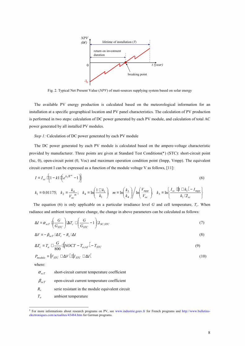
A typical cash-flow characteristic of this multi-sources system can be shown in the Fig. 3. The initial

investment of the system is completely made at time 0. So, on the lifetime of the installation T, the system is

profitable if the sum of future discounted cash-flows is higher than the initial investment. The breaking point

indicates that investment has been already amortized and PV installation could now be profitable. The period

time from initial point (initial year) to breaking point is the required return on investment duration (or pay-

back period). Obviously, the shorter amortization duration is obtained, the more system is economically

interesting. The downward jumps on the NPV curve are an increase in cost investment because of the

necessity to replace part of the installation (batteries, inverters). For the considered year, this replacement

decreases the linked cash-flow and thus NPV.

Analysis based on NPV method has two advantages. Firstly, it clearly points out if project is profitable or

not (positive NPV is sufficient to uncouple investment). Secondary, it indicates which time initial investment

is profitable. But NPV rule cannot explicitly show to decision maker how much financial attractiveness of the

proposed solution is. So, we complete with another index that attempts to identify the relationship between

the Benefits - Costs through a ratio, called Profitability Index (P.I), calculated as:

( )0

11

1.

I

NPV

I

INPV

I

i

CF

IPo

o

o

T

jj

j

+=+=

+=∑

= (5)

Logically, a ratio of 1.0 is the lowest acceptable measure on the index. The value smaller than 1.0 indicates

that the project is profitless (NPV<0). The higher value is, the more profit created by investment. For

example, calculation gives P.I = 1.5, it means NPV = 0.5, and every unit invested can create a value of 1.5.

3.2 Components' models specifications and constraints

3.2.1 PV generation model

8

breaking point

-I0

NPV

(k€)

t (year)

return on investment

duration

0

lifetime of installation (T)

Fig. 2. Typical Net Present Value (NPV) of muti-sources supplying system based on solar energy

The available PV energy production is calculated based on the meteorological information for an

installation at a specific geographical location and PV panel characteristics. The calculation of PV production

is performed in two steps: calculation of DC power generated by each PV module, and calculation of total AC

power generated by all installed PV modules.

Step 1: Calculation of DC power generated by each PV module

The DC power generated by each PV module is calculated based on the ampere-voltage characteristic

provided by manufacturer. Three points are given at Standard Test Conditions(∗) (STC): short-circuit point

(Isc, 0), open-circuit point (0, Voc) and maximum operation condition point (Impp, Vmpp). The equivalent

circuit current I can be expressed as a function of the module voltage V as follows, [11]:

−⋅−⋅= ⋅

111 2mVk

sc ekII (6)

( )

⋅−+⋅

=

=

+===sc

mppsc

oc

mpp

moc

Ik

IkIk

V

V

k

km

k

kk

V

kkk

1

13

4

3

1

14

421

1ln;lnln;

1ln;;01175.0

The equation (6) is only applicable on a particular irradiance level G and cell temperature, Tc. When

radiance and ambient temperature change, the change in above parameters can be calculated as follows:

STCSCSTC

cSTC

scT IG

GT

G

GI ,1 ⋅

−+∆⋅

⋅=∆ α (7)

IRTV scocT ∆⋅−∆⋅−=∆ β (8)

( ) STCrefaac TTNOCTG

TT −−⋅+=∆ ,800

(9)

( ) ( )IIVVP STCSTCmodule ∆+⋅∆+= (10)

where:

scTα short-circuit current temperature coefficient

ocTβ open-circuit current temperature coefficient

Rs serie resistant in the module equivalent circuit

Ta ambient temperature

§ For more informations about research programs on PV, see www.industrie.gouv.fr for French programs and http://www.bulletins-

electroniques.com/actualites/43484.htm for German programs.

9

NOCT Normal Operating Cell Temperature, specified to be 45°C

(at condition: irradiance G = 0.8 W/m2, ambient temperature Ta = 20°C, wind speed = 1 m/s)

Step 2: Calculation of AC power generated by the PV generator

The AC power generated by PV generator is the sum of production of all installed modules.

invertermodulemodulesPV PNP η⋅⋅= (11)

where inverterη : efficiency of inverter

By this way, PPV is the upper limit of the available power produced by PV generator.

3.2.2 Battery storage model

The lead-acid batteries are the most used in PV application. The storage system is known as a flexible

element of multi-sources system. It can store the total or surplus of production which is not used locally and

provide energy when needed. On the other hand, battery storage system constitutes a weak point due to short

lifetime period which are strongly influenced by many factors relating to the way it is operated such as:

discharge rate, partial cycling, charge factor, temperature ...etc. Therefore, two parts will be considered in

storage system modeling: operating model and ageing model.

Operation model

The battery storage system is characterized by its energy capacity ( maxS ), battery efficiency ( Bη ),

charging/discharging power capacity ( boutbin PP / ). We also use the battery charging and discharging rate

coefficients ( dchch rr / ) to define the maximal charging/discharging power capacity for each step time.

Knowing that charging and discharging are two processes quite independent and cannot be carried out at the

same time, it is necessary when the battery charges the discharging power must be null and contrarily. A new

variable α(t) is added, [12]:

( ) ( )

( )( ) ( )

≤≤−⋅∆

⋅⋅−

∆⋅⋅⋅≤≤

01

1

0

tPtt

rS

t

rSttP

boutB

dchmax

Bchmaxbin

αη

ηα

(12)

( ) ( )( )

( )( )

( )

→

≤≤∆

⋅⋅−

=

→=

→

=∆

⋅⋅≤≤→=

⇒

gdischargin isbattery

tPt

rS

tP

tif

charging isbattery

tP

t

rStP

tif

boutB

dchmax

bin

bout

Bchmaxbin

0

1

0

0

0

01

ηα

ηα

The relationship between storage level (SOC) and power flow in or out of the battery at any step time is:

( ) ( ) ( ) ( )tPtPtSOCtSOC boutbin −+=+1 (13)

10

To ensure the security, battery must be operated in a specific rang defined by maximal and minimal limit

of charge or discharge (SOCmax and SOCmin):

( ) maxmin SOCtSOCSOC ≤≤ (14)

Ageing model

The cumulative ampere-hour (Ah) throughput or Ah throughput method is used as basis for calculating

battery ageing. This method [13-16] assumes that there is a fixed amount of energy (called Ah throughput)

can be cycled through a battery before it requires replacement (regardless of the deep of individual cycles or

any other specific parameters to the way the energy is stored in or left out of the battery). The estimated Ah

throughput is derived from the depth of discharge versus cycles to failure curve provided by manufacturer:

( ){ } %

%maxy

xkk CFDoDSAveragethroughputAh ⋅⋅= (15)

where:

k: battery operating zone (specified depth of charge ranges between x% to y%)

DoDk: depth of charge k

CFk: cycles to failure (or number of cycles) if battery operates always at specific depth of charge k

An approximation is made by making the assumption that the product of the number of cycles by the depth

of discharge is constant. So the program can use the cycle life at a particular DOD, such as 50% to calculate

the Ah throughput cycled through the battery.

From these underlying assumptions, we can deduce the calculation of Ah throughput by:

%50%50max CFDoDSthroughputAh ⋅⋅= (16)

For example, a cycle life of 1050 of a 2.1 kWh battery at 50% DoD means that whenever 1102.5 ampere-

hour cycled through the battery, the battery is considered as used and needed to be replaced.

We notice that this simplistic approach minimizes the complexity of the problem considerably. Battery life

could then be estimated by the only accounting of exchanged energy thus avoiding the detection and the

counting of the effective cycles.

3.2.3 Grid model

The grid is modelled in the sizing optimization as a power source which is theoretically available

constantly, and represents an attribute of energy purchasing and selling policy. As the system is applied for

household application, the consumed grid power is only limited by the contracted power limit denoted Pgmax.

Pg(t) ≤ Pgmax (17)

In the connection architecture with one connecting point with the network, only excess PV power will be

sold to network. When the house consumes grid energy it cannot sell his solar energy. Conversely, when local

production (PV and battery) can satisfy the demand, surplus can be exported to network. So that:

z(t).Pg(t) = 0 (18)

Similarly to (12) and by introducing a decision binary variable β(t), the nonlinearity in (18) can be

transformed into linear form:

11

( ) ( ) ( )( ) ( )( )

−⋅≤≤⋅≤≤

tPtP

ttPtz

g

PV

ββ10

0

gmax

(19)

( ) ( ) ( )( )

( ) ( )( )

→

≤≤=

→=

→

=≤≤

→=

⇒

powergridconsumes house hetPtP

tztif

grid tosurplustheexports house hettP

tPtztif

gmaxg

g

PV

0

00

0

01

β

β

3.2.4 Controllable and no controllable loads model

Independently from electricity price paid, the consumption is composed by no controllable loads and

controllable loads. The load management possibility is considered in sizing optimization as follows:

It is supposed that the end users don’t mind the power consumption patterns if the purpose to use the

service is satisfied. For example, user expects that the service d is achieved at t = ad, the consumed energy

dchPe required should be maintained in an appropriate prescribed period τ = [ad-δd : ad] but consumed power

would be deferred.

( )dL

a

au

dL euP

d

dd

=∑−= δ

)( (20)

where:

δd is the time to realize the service d

However, the energy consumption must be the same as expected in the case without load management:

( )∑ +=∑t

NLPLPt

L tPtPtP )()()( (21)

3.3 Results analysis method

For this study, the problem is solved using the solver CPLEX implemented in Java environment. The

solution defines the the sizing values (Nmodules, Smax, Pgmax), the operation plan for sources and loads, and the

economical analysis value (NPV, P.I, the amortization duration) in function of the scenario given by problem

parameters as input data.

Sizing problem is to be solved by decision maker once before installation of system in order to determine

the optimal architecture, operation strategy and profit hope over its lifetime period. These calculations have

thus a great meaning in the feasibility and acceptability of the proposed solution. As said previously, the

obtained results depend on the scenario's parameters which could be sensitive and influenced by many

exogenous aspects. It is necessary for investor to identify the most important factors of influence and then, to

quantify their impacts on the solution. Several ones are cited, for exogenous factors as the renewable energy

support policy, the possible technology evolutions, the electricity market

12

Source : ADEME (2003)

5900

216229763621

75004512

0

2000

4000

6000

8000

2000 2005 2010 2015 2020 2030

(€/kWp)

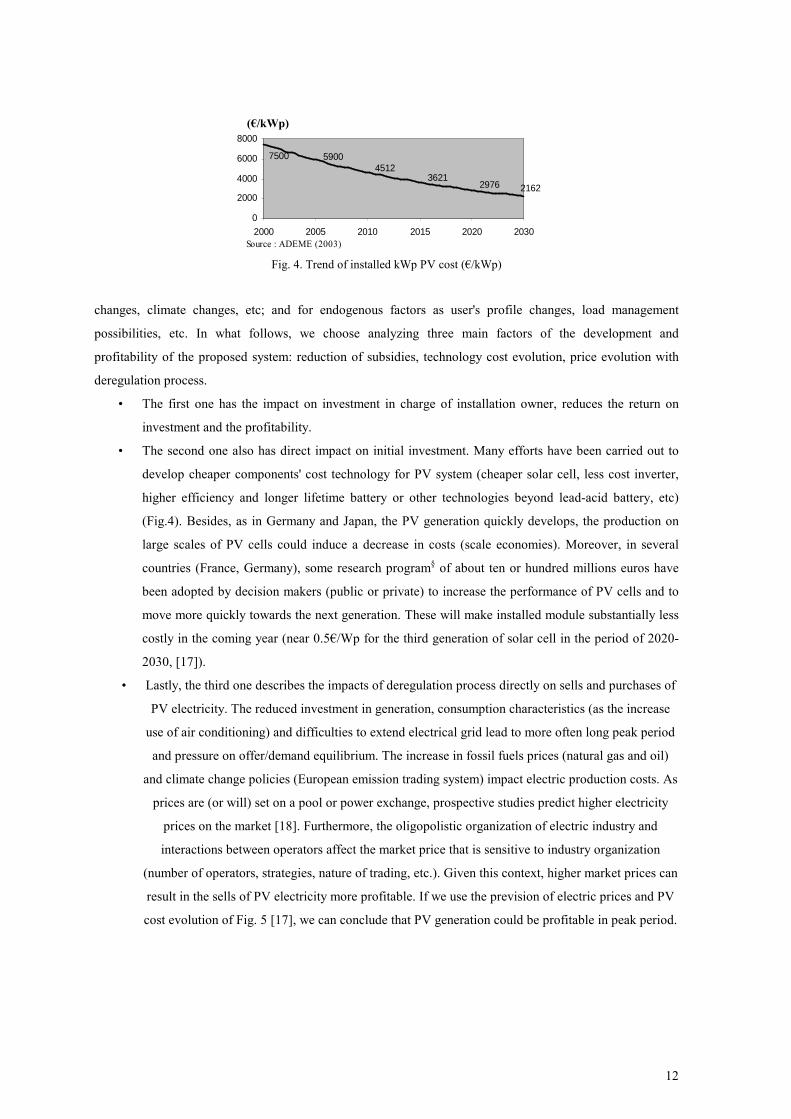
Fig. 4. Trend of installed kWp PV cost (€/kWp)

changes, climate changes, etc; and for endogenous factors as user's profile changes, load management

possibilities, etc. In what follows, we choose analyzing three main factors of the development and

profitability of the proposed system: reduction of subsidies, technology cost evolution, price evolution with

deregulation process.

• The first one has the impact on investment in charge of installation owner, reduces the return on

investment and the profitability.

• The second one also has direct impact on initial investment. Many efforts have been carried out to

develop cheaper components' cost technology for PV system (cheaper solar cell, less cost inverter,

higher efficiency and longer lifetime battery or other technologies beyond lead-acid battery, etc)

(Fig.4). Besides, as in Germany and Japan, the PV generation quickly develops, the production on

large scales of PV cells could induce a decrease in costs (scale economies). Moreover, in several

countries (France, Germany), some research program§ of about ten or hundred millions euros have

been adopted by decision makers (public or private) to increase the performance of PV cells and to

move more quickly towards the next generation. These will make installed module substantially less

costly in the coming year (near 0.5€/Wp for the third generation of solar cell in the period of 2020-

2030, [17]).

• Lastly, the third one describes the impacts of deregulation process directly on sells and purchases of

PV electricity. The reduced investment in generation, consumption characteristics (as the increase

use of air conditioning) and difficulties to extend electrical grid lead to more often long peak period

and pressure on offer/demand equilibrium. The increase in fossil fuels prices (natural gas and oil)

and climate change policies (European emission trading system) impact electric production costs. As

prices are (or will) set on a pool or power exchange, prospective studies predict higher electricity

prices on the market [18]. Furthermore, the oligopolistic organization of electric industry and

interactions between operators affect the market price that is sensitive to industry organization

(number of operators, strategies, nature of trading, etc.). Given this context, higher market prices can

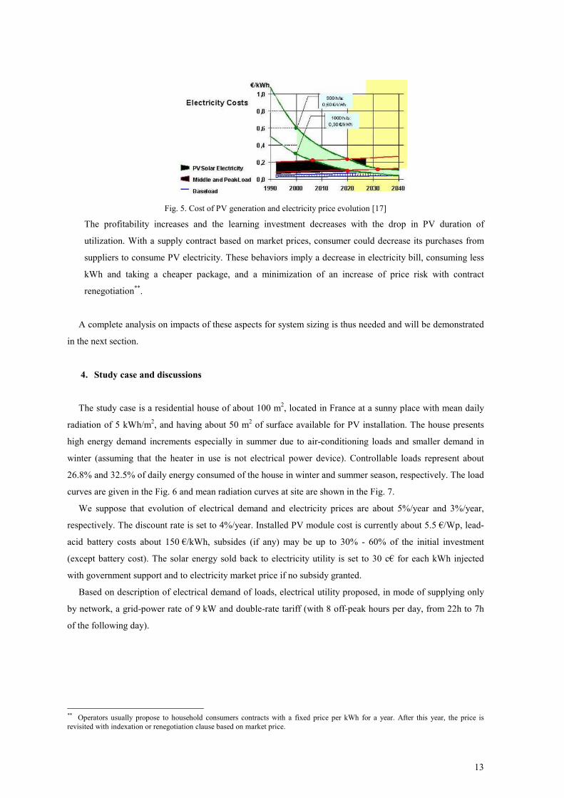
result in the sells of PV electricity more profitable. If we use the prevision of electric prices and PV

cost evolution of Fig. 5 [17], we can conclude that PV generation could be profitable in peak period.

13

Fig. 5. Cost of PV generation and electricity price evolution [17]

The profitability increases and the learning investment decreases with the drop in PV duration of

utilization. With a supply contract based on market prices, consumer could decrease its purchases from

suppliers to consume PV electricity. These behaviors imply a decrease in electricity bill, consuming less

kWh and taking a cheaper package, and a minimization of an increase of price risk with contract

renegotiation**.

A complete analysis on impacts of these aspects for system sizing is thus needed and will be demonstrated

in the next section.

4. Study case and discussions

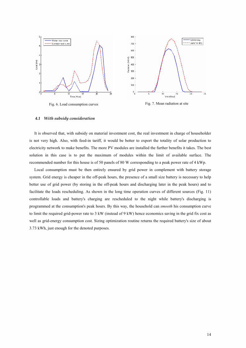
The study case is a residential house of about 100 m2, located in France at a sunny place with mean daily

radiation of 5 kWh/m2, and having about 50 m

2 of surface available for PV installation. The house presents

high energy demand increments especially in summer due to air-conditioning loads and smaller demand in

winter (assuming that the heater in use is not electrical power device). Controllable loads represent about

26.8% and 32.5% of daily energy consumed of the house in winter and summer season, respectively. The load

curves are given in the Fig. 6 and mean radiation curves at site are shown in the Fig. 7.

We suppose that evolution of electrical demand and electricity prices are about 5%/year and 3%/year,

respectively. The discount rate is set to 4%/year. Installed PV module cost is currently about 5.5 €/Wp, lead-

acid battery costs about 150 €/kWh, subsides (if any) may be up to 30% - 60% of the initial investment

(except battery cost). The solar energy sold back to electricity utility is set to 30 c€ for each kWh injected

with government support and to electricity market price if no subsidy granted.

Based on description of electrical demand of loads, electrical utility proposed, in mode of supplying only

by network, a grid-power rate of 9 kW and double-rate tariff (with 8 off-peak hours per day, from 22h to 7h

of the following day).

** Operators usually propose to household consumers contracts with a fixed price per kWh for a year. After this year, the price is

revisited with indexation or renegotiation clause based on market price.

14

Fig. 6. Load consumption curves

Fig. 7. Mean radiation at site

4.1 With subsidy consideration

It is observed that, with subsidy on material investment cost, the real investment in charge of householder

is not very high. Also, with feed-in tariff, it would be better to export the totality of solar production to

electricity network to make benefits. The more PV modules are installed the further benefits it takes. The best

solution in this case is to put the maximum of modules within the limit of available surface. The

recommended number for this house is of 50 panels of 80 W corresponding to a peak power rate of 4 kWp.

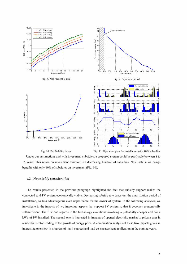
Local consumption must be then entirely ensured by grid power in complement with battery storage

system. Grid energy is cheaper in the off-peak hours, the presence of a small size battery is necessary to help

better use of grid power (by storing in the off-peak hours and discharging later in the peak hours) and to

facilitate the loads rescheduling. As shown in the long time operation curves of different sources (Fig. 11)

controllable loads and battery's charging are rescheduled to the night while battery's discharging is

programmed at the consumption's peak hours. By this way, the household can smooth his consumption curve

to limit the required grid-power rate to 3 kW (instead of 9 kW) hence economics saving in the grid fix cost as

well as grid-energy consumption cost. Sizing optimization routine returns the required battery's size of about

3.73 kWh, just enough for the denoted purposes.

15

Fig. 8. Net Present Value

Unprofitable zone

Fig. 9. Pay-back period

Fig. 10. Profitability index Fig. 11. Operation plan for installation with 40% subsidies

Under our assumptions and with investment subsidies, a proposed system could be profitable between 8 to

15 years. This return on investment duration is a decreasing function of subsidies. New installation brings

benefits with only 10% of subsidies on investment (Fig. 10).

4.2 No subsidy consideration

The results presented in the previous paragraph highlighted the fact that subsidy support makes the

connected grid PV system economically viable. Decreasing subsidy rate drags out the amortization period of

installation, so less advantageous even unprofitable for the owner of system. In the following analyses, we

investigate in the impacts of two important aspects that support PV system so that it becomes economically

self-sufficient. The first one regards in the technology evolutions involving a potentially cheaper cost for a

kWp of PV installed. The second one is interested in impacts of opened electricity market to private user in

residential sector leading to the growth of energy price. A combination analysis of these two impacts gives an

interesting overview in progress of multi-sources and load co-management application in the coming years.

16

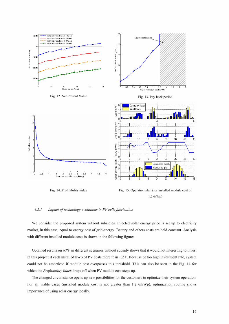
Fig. 12. Net Present Value

Unprofitable zone

Fig. 13. Pay-back period

Fig. 14. Profitability index Fig. 15. Operation plan (for installed module cost of

1.2 €/Wp)

4.2.1 Impact of technology evolutions in PV cells fabrication

We consider the proposed system without subsidies. Injected solar energy price is set up to electricity

market, in this case, equal to energy cost of grid-energy. Battery and others costs are held constant. Analysis

with different installed module costs is shown in the following figures.

Obtained results on NPV in different scenarios without subsidy shows that it would not interesting to invest

in this project if each installed kWp of PV costs more than 1.2 €. Because of too high investment rate, system

could not be amortized if module cost overpasses this threshold. This can also be seen in the Fig. 14 for

which the Profitability Index drops-off when PV module cost steps up.

The changed circumstance opens up new possibilities for the customers to optimize their system operation.

For all viable cases (installed module cost is not greater than 1.2 €/kWp), optimization routine shows

importance of using solar energy locally.

17

Although a part of controllable loads needs to be rescheduled to the night to profit the cheaper grid-energy

tariff in off-peak hours, the more important part is better to be removed to midday hours (from 10 am to 15

pm) where solar energy is prospered. Since injected energy selling price is equal to grid-energy buying tariff,

there is no interest to storing solar energy to resell latter. As long as it is not consumed locally, surplus will be

sold to electrical network. In this configuration, battery plays clearly the role of flexible element of system by

charging grid-energy as well as a limited solar energy just for load management purpose. For this reason,

grid-power subscription is also limited at 3 kW and obtained battery's size is 3.73 kWh.

As selling of the surplus of solar energy brings more benefit for system to accelerate the amortization

duration. It is recommended to install as much modules as possible in the limit of available surface (here, 50

modules equivalent to 4 kWp).

We can conclude that if investment costs of PV are lower and with the assumption that electric PV

generation is sold to the grid at the market price, the proposed system could show profit for a household

consumer. In the system operation consideration, we can see that user can take further benefit if PV electricity

is more consumed locally.

4.2.2 Impacts of the deregulated electricity market

Impact of opened electricity market to user of residential sector is analyzed in this paragraph. For this

purpose, installed modules and others cost take values as in current situation (c.f. 4.1). Energy prices vary

from 10 c€/kWh (current grid-energy price applied for residential user) to 1 €/kWh. Injected solar energy sold

to network at the same tariff of grid-energy cost.

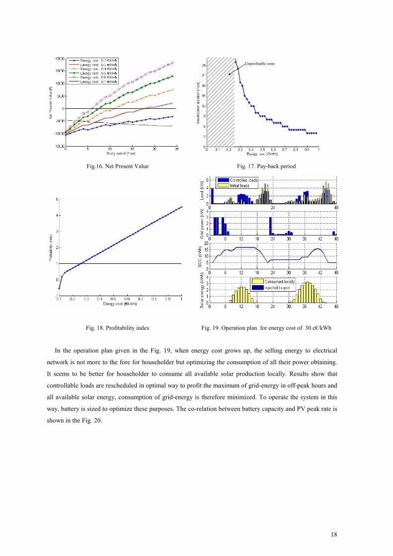
Analysis on NPV and P.I indicates that in the current condition (10 c€/kWh), the project is completely

unprofitable. As shown in Fig. 16, if energy prices are lower, consumer has not incentives to make investment

on the proposed system. It does not produce with the system, so costly, and consumes grid energy. Thus,

cash-flows are negatives and the NPV is always decreasing. The system is unprofitable. This confirms once

again the importance of actual government's subsidy for connected-grid PV system to promote the

development of solar energy. However, if energy cost increases (greater than 25 c€/kWh), the system can be

self-amortized in spite of the high investment rate.

18

Unprofitable zone

Fig.16. Net Present Value Fig. 17. Pay-back period

Fig. 18. Profitability index Fig. 19. Operation plan for energy cost of 30 c€/kWh

In the operation plan given in the Fig. 19, when energy cost grows up, the selling energy to electrical

network is not more to the fore for householder but optimizing the consumption of all their power obtaining.

It seems to be better for householder to consume all available solar production locally. Results show that

controllable loads are rescheduled in optimal way to profit the maximum of grid-energy in off-peak hours and

all available solar energy, consumption of grid-energy is therefore minimized. To operate the system in this

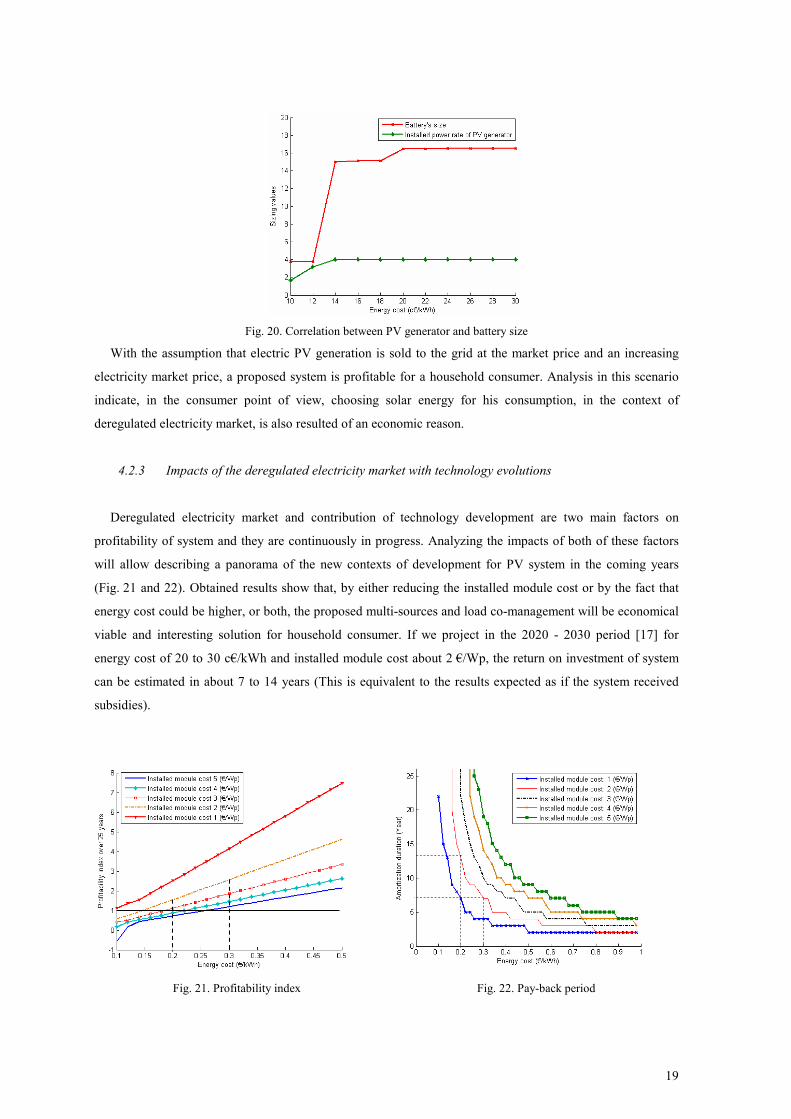
way, battery is sized to optimize these purposes. The co-relation between battery capacity and PV peak rate is

shown in the Fig. 20.

19

Fig. 20. Correlation between PV generator and battery size

With the assumption that electric PV generation is sold to the grid at the market price and an increasing

electricity market price, a proposed system is profitable for a household consumer. Analysis in this scenario

indicate, in the consumer point of view, choosing solar energy for his consumption, in the context of

deregulated electricity market, is also resulted of an economic reason.

4.2.3 Impacts of the deregulated electricity market with technology evolutions

Deregulated electricity market and contribution of technology development are two main factors on

profitability of system and they are continuously in progress. Analyzing the impacts of both of these factors

will allow describing a panorama of the new contexts of development for PV system in the coming years

(Fig. 21 and 22). Obtained results show that, by either reducing the installed module cost or by the fact that

energy cost could be higher, or both, the proposed multi-sources and load co-management will be economical

viable and interesting solution for household consumer. If we project in the 2020 - 2030 period [17] for

energy cost of 20 to 30 c€/kWh and installed module cost about 2 €/Wp, the return on investment of system

can be estimated in about 7 to 14 years (This is equivalent to the results expected as if the system received

subsidies).

Fig. 21. Profitability index Fig. 22. Pay-back period

20

5. Conclusions

We are in a context of solar energy managing. We come out of the current idea that, with feed-in tariffs

and obligatory purchases, a consumer has interest to invest in the maximum capacity of photovoltaic

production and then, he sells all produced quantities to the network utilities.

Here, we assume a future context in which feed-in tariffs and purchase obligations, are finished. All

photovoltaic generation is consumed or sold on the market at the market price. Household consumers sign

market price contract, with indexation and renegotiations in prices. So, the importance of global household

energy in general and management strategies of photovoltaic electricity in particular appear. The objective of

this paper is to propose a new method of optimal supplying system sizing and household energy management.

The mains advantages of this method are:

• optimizing, based on MLP the components' size of connected-gird supplying multi-source system,

• optimizing the operation of system, (source and load management)

• providing a optimization tool, based on NPV and P.I methods, to analyze the economic viability of

PV system as function of scenarios defined by problem parameters

The obtained results could give an overview on the PV system development towards the near and

medium-term future. It is shown that, in the current period, the incentives policies are necessary to promote

renewable energies because the return on investment duration is very long (or do not exist) if we only

consider current market price and investment costs. So, interest to build a PV system without these policies,

do not exist. But, with the previsions of market price evolutions, market price contracts negotiation and

contribution of technology developments, the problematic will change. Under assumptions close to previsions

of PV development and electricity market design that we anticipate up to the period 2020-2030, it is

estimated that the system should be profitable with a relative independent regarding public subsidy. This

becomes a good assessment for household customer to shift their consumption more intelligent and to be

willing to invest in lower environment impacts energy productions.

References

[1] Jäger-Waldau A. Photovoltaics and renewable energies in Europe. Renewable and Sustainable Energy Reviews. 2007; 11(7) :

1414-1437

[2] Saenz de Miera G, Del Rıo Gonzalez P, Vizcaıno I. Analysing the impact of renewable electricity support schemes on power

prices: The case of wind electricity in Spain. Energy Policy. 2008; 36: 3345– 3359

[3] Department for Communities and Local Government, 2007, “The future of the Code for Sustainable Homes : Making a rating

mandatory”, www.communities.gov.uk

[4] B. Burger, R. Rüthe. “Site-dependent system performance and optimal inverter sizing of grid-connected PV systems”.

Photovoltaic Specialists Conference, 2005. Conference Record of the Thirty-first IEEE 3 - 7 Jan. 2005, pp1675 - 1678.

[5] Wurtz, S. Bacha, T.T.Ha. Pham, G. Foggia, D. Roye, G. Warkosek. (2007). Optimal Energy Management in buildings: sizing,

anticipative and reactive management. Energy Management system Workshop – Torino 24 - 25 May 2007

[6] J.D. Moldol, Y.G. Yohanis, B.Norton. “Optimal sizing of array and inverter for grid-connected photovoltaic systems”. Solar

Energy, Volume 80 (2006) 1517-1539.

21

[7] J.C. Hernández, P.G. Vidal, G. Almonacid. “Photovoltaic in grid-connected buildings: sizing and economic analysis”. Renewable

Energy, Volume 15, Issues 1-4, September-December 1998, pp. 562-565

[8] Fernández-Infantes, J. Contreras, J. L. Bernal-Agustín. “Design of grid connected PV systems considering electrical, economical

and environmental aspects: A practical case”. Renewable Energy, Volume 31, Issue 13, October 2006, pp.2042-2062

[9] J.A. Momoh, “Electric Power System Applications of Optimization”, Marcel Dekker, Inc. 2001.

[10] Bernal-Agustin J.L, Dufo-Lopez R. Economical and environmental analysis of grid connected photovoltaic systems in Spain.

Renewable Energy. 2006 ; 31 : 1107–1128

[11] Frederick M. Ishengoma, Lars E. Norum. “Design and implementation of a digitally controlled stand-alone photovoltaic supply”.

Nordic Workshop on Power and Industrial Electronics. NORPIE, 12 - 14 August 2002.

[12] D-L. Ha. Un système avancé de gestion d'énergie dans le bâtiment pour coordonner production et consommation. Ph.D.

dissertation, Department Electrical Engineering. Institut National Polytechnique de Grenoble (INP Grenoble), Grenoble,

September,2007

[13] H. Bindner, T. Cronin, P. Lundsager, J.F. Manwell, U. Abdulwahid, I. Baring-Gould. “Lifetime Modelling of Lead Acid

Batteries”. Project ENK6-CT-2001-80576. Risø National Laboratory, Roskilde, Denmark, April 2005.

[14] G.Robin, O.Gergaud, H. Ben Ahmed, N Barnard, B. Multon. “Problématique du stockage d'énergie situé chez le consommateur

connecté au réseau”. EF'2003 - Electrotechnique du Futur - 9 & 10 Décembre 2003, Supélec, Gif-sur-Yvette, France.

[15] A. Cherif, M. Jrairi, A. Dhouid. “A battery ageing model used in stand-alone PV systems”. Journal of Power Sources 112, 2002,

pp. 49-53

[16] “Detailed Evaluation of Renewable Energy Power System Operation: A Summary of the European Union Hybrid Power System

Component. Benchmarking Project”. Available electronically at http://www.osti.gov/bridge

[17] ADEME, 2003, « Les Energies et Matières Premières Renouvelables en France - Situation et perspectives de développement dans

le cadre de la lutte contre le changement climatique”, march, 26, 2003, part 2, available on www.debat-

energie.gouv.fr/site/pdf/enr-2.pdf

[18] W. Lise and G. Kruseman, 2006, “Long-term price and environmental effects in a liberalised electricity market”, Energy

Economics, In press