1

Optimal Portfolio Rebalancing Strategy:

Evidence from Finnish

Stocks

Savage, Akinwunmi

Supervisor: Henrik Sällberg

Master’s Thesis in Business Administration, MBA programme

2010

2

Abstract

Portfolio rebalancing is an established concept in portfolio management and investing

generally. Assets within a portfolio have different return and risk prospects, and this

inevitably leads them to drift away from their initial allocation weights overtime. Portfolio

rebalancing is arguably the only method by which such assets can be reset to their initial

weights, thus ensuring the portfolio reflects the risk appetite of the investor.

Like many other concepts and practices in finance, portfolio rebalancing is a somewhat

contentious topic, and many studies have sought to unearth optimal methods or strategies for

rebalancing portfolios. This study also entered the fray of portfolio rebalancing research by

analysing three broad strategies to determine which would be most optimal. The rebalancing

strategies evaluated were: Calendar interval rebalancing (annually, half-yearly, quarterly, and

monthly); threshold percentage trigger rebalancing (where a pre-established percentage is

used to determine when rebalancing should be done); and a hybrid approach incorporating

both the latter and the former.

An equally weighted portfolio of 19 Finnish stocks from the Helsinki OMX25 index was used

in the analysis, and the study period spanned May, 2000 to April, 2010. The results of the

analysis showed that rebalancing provides rewards in terms of improved returns compared to

not rebalancing at all. However, none of the 54 sub-strategies analysed under the three broad

categories generated enough net of costs returns to be considered exceptionally optimal. Thus,

rebalancing is best implemented when risk control and the psychological benefits associated

with active portfolio management are desired. The above notwithstanding, arguably the most

formidable returns were generated with a threshold of ±50-60% (implying that the portfolio is

rebalanced when any asset weight drops to 2.10-2.63% or rises to 7.89-8.42%). This strategy

set-off a relatively small number of rebalances, implying relatively low costs. It was also

better than all other strategies, and far superior to choosing not to rebalance at all.

ii

Table of contents

Abstract ................................................................................................................................ ii

List of Tables ...................................................................................................................... iv

List of Figures .......................................................................................................................v

List of Equations ................................................................................................................ vi

1 Introduction ....................................................................................................................1

1.1 Background .......................................................................................................................1

1.2 Motivation ..........................................................................................................................2

1.3 Research purpose.............................................................................................................3

1.4 Contribution .......................................................................................................................4

1.5 Scope and limitations .......................................................................................................5

2 Asset and Portfolio management ................................................................................6

2.1 Asset Management ...........................................................................................................6

2.2 Modern Portfolio Theory ...................................................................................................8

2.2.1 Efficient Frontier ........................................................................................................ 10

2.2.2 Tobin’s two-fund separation ...................................................................................... 10

2.3 Portfolio management .................................................................................................... 11

2.4 Asset allocation ............................................................................................................... 12

2.4.1 Strategic asset allocation ........................................................................................... 14

2.4.2 Tactical asset allocation ............................................................................................. 14

2.5 Portfolio rebalancing ....................................................................................................... 14

2.5.1 Portfolio rebalancing example ................................................................................... 15

2.5.2 Pros and cons of rebalancing...................................................................................... 17

2.5.3 Rebalancing strategies ............................................................................................... 18

3 Review of previous studies ........................................................................................ 19

3.1 Does Portfolio Rebalancing Help Investors Avoid Common Mistakes?..................... 19

3.1.1 Empirical Analysis ...................................................................................................... 20

3.2 Rebalancing Diversified Portfolios of Various Risk Profiles ........................................ 21

3.2.1 Empirical Analysis ...................................................................................................... 22

3.3 The Benefits of Rebalancing .......................................................................................... 23

iii

3.3.1 Empirical Analysis ...................................................................................................... 24

3.4 Alternative Portfolio Rebalancing Strategies Applied to Sector Funds ...................... 27

3.4.1 Empirical Analysis ...................................................................................................... 27

3.5 Literature review summary ............................................................................................. 28

4 Data and Research Methodology.............................................................................. 31

4.1 Description of Data ......................................................................................................... 31

4.2 Assumptions .................................................................................................................... 32

4.3 Research Method............................................................................................................ 33

4.3.1 Rebalancing based on calendar intervals .................................................................... 34

4.3.2 Rebalancing based on initial allocation weight drifts .................................................. 34

4.3.3 Rebalancing based a hybrid of calendar and weight drifts strategies .......................... 35

5 Empirical results.......................................................................................................... 36

5.1 Calendar rebalancing ..................................................................................................... 36

5.2 Percentage threshold rebalancing ................................................................................. 38

5.3 Hybrid rebalancing strategy ........................................................................................... 39

6 Conclusions and Recommendations ........................................................................ 41

References ......................................................................................................................... 45

Appendix A ......................................................................................................................... 47

Appendix B ......................................................................................................................... 48

Appendix C ......................................................................................................................... 49

Appendix D ......................................................................................................................... 50

Appendix E ......................................................................................................................... 51

iv

List of Tables

Table 2.1: Portfolio Rebalancing Example ............................................................................ 15

Table 3.1: Annual Rebalancing vs Chase Portfolio ............................................................... 21

Table 3.2: Five portfolios representing various risk profiles .................................................. 22

Table 3.3: Average Asset Exposures at Different Rebalancing Intervals ............................... 25

Table 3.4: Actual Net Returns and Risk Results for A 5% Rebalancing Interval (1987 – 2000)

............................................................................................................................................. 26

Table 3.5: Summary of Literature Review ............................................................................ 30

Table 4.1: Descriptive statistics of research data ................................................................... 33

Table 5.1: Calendar Rebalancing Strategy ............................................................................ 37

Table 5.2: Percentage Trigger Rebalancing Strategy ............................................................. 38

Table 5.3: Hybrid (Percentage & Monthly Monitoring) Strategy........................................... 39

Table 6.1: Rankings of the upper quartile strategies over 3 time periods ............................... 43

v

List of Figures

Figure 2.1: The Portfolio Management Process ..................................................................... 11

Figure 4.1: OMX Helsinki 25 Index September, 2001 – April, 2010 ..................................... 31

Figure 5.1: Cost Implication of Calendar Rebalancing .......................................................... 37

Figure 5.2: Cost Implication of Percentage Threshold Rebalancing....................................... 39

Figure 5.3: Cost Implication of Monthly Hybrid Rebalancing ............................................... 40

vi

List of Equations

Equation 2.1: Asset Expected Return ......................................................................................6

Equation 2.2: Asset Variance ..................................................................................................7

Equation 2.3: Asset Standard Deviation/Volatility ..................................................................7

Equation 2.4: Coefficient of Variation ....................................................................................7

Equation 2.5: Portfolio Expected Return .................................................................................8

Equation 2.6: Asset Covariance ..............................................................................................9

Equation 2.7: Asset Correlation ..............................................................................................9

Equation 2.8: Portfolio Variance .............................................................................................9

Equation 2.9: Portfolio Standard Deviation .............................................................................9

Equation 4.1: Return Calculated from Asset Closing Prices .................................................. 32

1

1 Introduction

1.1 Background

The importance of portfolio rebalancing in portfolio management is clear and unquestionable.

Eakins and Stansell (2007) highlight the significance of this concept very aptly by asserting

that, “it is a widely recognised tenet of finance that investors must rebalance their portfolios at

regular intervals to prevent becoming over invested in one type of security”. But how regular

or irregular should this interval be? This question unveils the inspiration behind papers of this

nature – what is the most appropriate or optimal strategy for rebalancing? Masters (2003)

buttresses this point further by stating “while the benefits of rebalancing are generally

acknowledged, there is little agreement on the right rebalancing strategy”.

In the quest to seek out the answer to the question stated above, academics, computational

finance experts, mathematicians, and software programmers alike have, on their own and at

the behest of mostly large institutional investors, researched complex algorithms and models

(Sun et al, 2006 and Y. Fang et al, 2006).

It is noteworthy however, that since the efficient market hypothesis implies that it ought to be

theoretically impossible to beat the market based on analysing historical returns alone, it can

be asserted rather confidently that a rebalancing strategy based on complex models and

computational analysis, implemented ex ante, has about as much chance of ensuring the

generation of satisfactory risk-adjusted returns as does a strategy based on analysing historical

data, irrespective of how complex or simple the analysis might be.

From the above, it follows that individuals and small institutional investors, without the

financial wherewithal of their more well-off counterparts, can also be effective at rebalancing

their portfolios. Hence, the focal objective of this paper is to determine if, by simple and easy

to replicate means, an optimal portfolio rebalancing strategy can identified based on evidence

from Finnish securities.

2

1.2 Motivation

The Institute of Business and Finance provides training in mutual fund advisory services and

awards the Certified Fund Specialist® (CFS®) designation, amongst a number of other

designations. Alongside a wide range of training literature, they consistently furnish current

and prospective designees with research findings regarding mutual funds particularly and

investing generally. One of such findings claims that rebalancing portfolios every 44 months

is the most optimal strategy to adopt. Advisors with the CFS® designation are expected to use

this “knowledge” in their practices, and of course get paid for it. The rebalancing interval of

44 months stated above, though contestable, is even less egregious than other circumstances

where advisors adopt a largely unproven rule-of-thumb in determining how often to rebalance

their clients‟ portfolios. Some adopt an arbitrary time interval and use it without objective

evidence to prove that it is optimal.

It is well known that consultants typically justify their fees by analysing the needs of their

clients and then proposing ideas or solutions that the client is often made to believe they are

unable to come up with on their own. In the same vein, fund managers and financial advisors

justify their fees by rendering services that the average patron is supposedly unqualified or

unable to provide unassisted.

However, a consideration of the unsettled debate about whether or not the majority of mutual

funds are able to beat the market consistently – and by implication, whether fund managers

and their fees are indeed justified – leads one to question if a careful examination of the

services/advice typically rendered by financial advisors would not unveil some that are

merely speculative or perhaps even replicable by the average investor, and thus somewhat

unjustified from a fee collection standpoint.

It has to be said that there are indeed a number of reasons why engaging the services of a fund

manager or financial advisor is a good idea. Aside from the technical knowhow and

experience these professionals undoubtedly possess, there are also savings from scale

economies that their practices enjoy and can pass on to their clients. Thus, for the most part, a

good part of their fees are arguably justified.

3

On the other hand, certain services are perhaps not particularly special from a logical

standpoint. The case in point is portfolio rebalancing. As already stated in the introduction,

the efficient market hypothesis rightfully asserts that any analysis hinged on historical returns

is, or should be, as good as the next. The motivation for this paper was birthed upon this

assertion. As such, in a nutshell, this paper seeks to determine if there is a rebalancing

strategy that is most beneficial to investors.

1.3 Research purpose

As alluded to already, and as opined by Buetow et al (2002) as well as all the other studies

covered in the literature review herein, adopting portfolio rebalancing is clearly more

beneficial than not adopting it. Thus, this paper‟s primary research focus is on the question

below:

What is the most optimal or beneficial strategy for rebalancing portfolios?

The research question above implies that this study will seek to determine, by empirical

means, what measurable benefits, if any, accrue to different portfolio rebalancing strategies.

Thereafter, the evaluated strategies will be compared based on the measured benefits. If a

rebalancing strategy proves to be the most beneficial, then the study will also seek to

determine whether or not the identified strategy is consistent with the findings from previous

research (and how) the strategy can be implemented by the average investor.

In order to establish whether or not portfolio rebalancing is beneficial, three main portfolio

rebalancing strategies will be compared to one another over a ten-year time period. The three

strategies are:

1. Rebalancing at intervals of time (monthly, quarterly, semi-annually, and annually),

2. Rebalancing when any asset class exceeds or falls below its initial allocation weight

by a pre-established threshold percentage (e.g. 5%, 10%, 20%, etc), and

3. A hybrid of both the aforementioned strategies, i.e., rebalancing whenever an asset

class exceeds or falls below its asset allocation weight, by a pre-established threshold,

after a specific time interval.

4

The strategies above will be applied to Finnish stock data and, because of time and resource

constraints, only one equally-weighted portfolio will be evaluated using the three strategies

listed above. The determination of whether or not a strategy is optimal or beneficial will be

based on an evaluation of the return, risk, and risk per unit of return of the strategy, as well as

the cost implications of implementing the strategy. Consequently, if any strategy proves to be

optimal, it will be compared to the findings from previous research in order to determine if

there is some degree of consistency. Further elaboration about the data and research

methodology will be presented in the fourth chapter.

1.4 Contribution

Firstly, noting that majority of studies of this nature have been carried out using U.S. data,

this paper seeks to make a modest contribution by using relatively less researched1 Finnish

data instead. Secondly, this research intends to reach conclusions that will be valuable to

investors and portfolio managers alike. It is expected that at the end of the study, the results

will either further buttress, or refute, current opinions about the practice of portfolio

rebalancing. As a by-product, considering the fact that rebalancing is an active portfolio

management strategy, if an optimal rebalancing strategy is identified, it will point out

somewhat whether active investing is indeed beneficial and what extent of involvement is

required.

Also, aside from the sheer differences between the sizes of the U.S. and Finnish economies

which arguably warrant separate studies, some researchers, such as Liljeblom et al (1997),

have found that the correlation between international markets have been low2, further pointing

out the fact that market situations across borders are unique. Reilly and Brown (2002: p. 59)

in their book on Investment Analysis and Portfolio Management, compared asset allocation

strategies in different countries and asserted that “national differences can explain much of the

divergent portfolio strategies”. They opine further that non-U.S. investors are expected to

1 This is especially true when it concerns studies published in English based on Finnish data. 2 Their study reports the correlation between the U.S. and Finnish markets to be a mere 0.22. Clearly, considering

that the study was done in 1997, one can argue that this result is outdated. However, a more recent study by

American Century Investments in April 2007 shows that the correlation between the S&P500 and the EAFE index

(Finland is part of the index) historically ranged between 0.11 and 0.93 over 37 years, averaged at 0.55, peaked in

2004, and has been on the decline since then.

5

make portfolio decisions that are dissimilar to the decisions of their U.S. counterparts because

“they face different social, economic, political, and tax environments”. The claim above

provides further inspiration for seeking to determine the most optimal rebalancing strategy

based on evidence from Finland.

1.5 Scope and limitations

Expectedly, the study is saddled with its fair share of limitations. Resource limitations imply

that this research will only make recourse to public data sources. In addition, time constraints

militated against a more thorough study. Thus, the decision to analyse only a simple equally-

weighted portfolio of disaggregated stocks was made because of the constraint above more

than anything else. With regards to evaluating the cost and benefits of the different

rebalancing strategies examined herein, whilst the benefits in terms of returns to the portfolio

will be exact and deduced from the empirical analysis, on the other hand, a commonsensical

approach will be applied to cost related inferences and estimates instead. Also, the intention to

cover only the last ten years of Finnish stock data necessitates a caveat; the conclusions

reached herein might not necessarily be foolproof or expected to hold with all certainty over a

different ten-year period.

6

2 Asset and Portfolio management

2.1 Asset Management

The management of any asset refers to the process of selecting the asset, the method of

maintaining or handling the asset over the duration of possession, and the means of disposing

the asset, if need be. In order to facilitate selection, a determination of the value of the asset in

question is a necessary first step. The duration of possession, or the holding period, is

influenced by a host of factors; for example, the type of investor, the investor‟s attitude to

risk, and the perceived or actual benefits derived from the asset. Finally, disposal is often

carried out in order to obtain pecuniary and/or other strategic benefits or even to stem losses

in some instances.

As with any decision making activity, none of the subparts of the asset management process

highlighted above can be properly carried out without adequate information or knowledge

about the nature of the asset before and during ownership or possession. In order to aid the

selection process, as investors are often faced with a plethora of assets that they can choose

from, the information obtained about an asset must of necessity foster its comparability with

other assets. As regards marketable assets or securities, the most traditional and perhaps the

two most critical inputs that aid decision making are the return prospects of the asset and its

risk characteristics.

The return prospects of an asset or its expected return, denoted , can be computed if its

probability distribution or the likelihood of occurrence of its payoff under different economic

scenarios is known. With this method, the expected return is calculated as the weighted

average of the product of the return probability and the probable returns as below:

Equation 2.1: Asset Expected Return

7

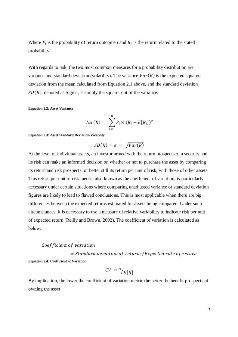
Where is the probability of return outcome i and is the return related to the stated

probability.

With regards to risk, the two most common measures for a probability distribution are

variance and standard deviation (volatility). The variance is the expected squared

deviation from the mean calculated from Equation 2.1 above, and the standard deviation

, denoted as Sigma, is simply the square root of the variance.

Equation 2.2: Asset Variance

Equation 2.3: Asset Standard Deviation/Volatility

At the level of individual assets, an investor armed with the return prospects of a security and

its risk can make an informed decision on whether or not to purchase the asset by comparing

its return and risk prospects, or better still its return per unit of risk, with those of other assets.

This return per unit of risk metric, also known as the coefficient of variation, is particularly

necessary under certain situations where comparing unadjusted variance or standard deviation

figures are likely to lead to flawed conclusions. This is most applicable when there are big

differences between the expected returns estimated for assets being compared. Under such

circumstances, it is necessary to use a measure of relative variability to indicate risk per unit

of expected return (Reilly and Brown, 2002). The coefficient of variation is calculated as

below:

Equation 2.4: Coefficient of Variation

By implication, the lower the coefficient of variation metric the better the benefit prospects of

owning the asset.

8

2.2 Modern Portfolio Theory

The phrase “Portfolio Management” is inextricably linked with the name Harry Markowitz.

This is due, in no small part, to the fact that his 1952 essay on “Portfolio Selection” laid the

foundation for what is referred to today as “Modern Portfolio Theory” (MPT). In addition to

other achievements, Markowitz is noted to have drawn attention to the fact that investors are

generally mean-variance optimisers, and they constantly seek “the lowest possible return

variance for any given level of mean (or expected) return”. He then proceeded to prove that

portfolio diversification provided a means for achieving this goal, by showing that risk

(standard deviation) could be reduced with little or no change in a diversified portfolio‟s

returns, and vice versa.

With regards to evaluating the performance of portfolios, the MPT has furnished portfolio

managers and investors alike with a host of tools which has led to a fundamental shift in the

way assets were ranked and selected over time. In the past, as stated in the penultimate

paragraph, assets were likely to have been evaluated and classed solely on their income or

return and risk prospects. This is no longer the case, as hardly any proper evaluation of assets

is carried out today without consideration of the idiosyncratic and systematic risk borne by

individual assets, as well as a host of other risk-adjusted measures of asset performance. More

than anything else, the MPT showed that, unlike in the case of a single asset, whilst the

expected return of a portfolio is the weighted average of the expected returns of its constituent

parts, the variance and volatility are not. In order to determine a portfolio‟s variance and

volatility, an estimate of the degree of co-movement among the assets in the portfolio is a key

input. The equations for calculating a portfolio‟s expected return, covariance, variance, and

volatility are shown below:

Equation 2.5: Portfolio Expected Return

Where is the expected return to the portfolio; is the expected return to asset i

within the portfolio; is the allocated weight of asset i. The weights of the portfolio are

determined from the ratio of the monetary allocation of an individual asset to the entire funds

available for investing. Thus, if 0.20€ out of 1€ is allocated to asset i, then its weight within

9

the portfolio would be . Expectedly, all the weights of the constituent parts of

a portfolio must sum up to 1.

Equation 2.6: Asset Covariance

Where is the covariance between the returns to asset i and asset j; and are

actual return observations; and are the mean returns calculated from the actual

return observations of assets i and j.

Equation 2.7: Asset Correlation

Where is the correlation coefficient between assets i and j: is the

covariance, as calculated from Equation 2.6 above; and are the volatilities or

standard deviation of assets i and j as calculated with Equation 2.3.

Equation 2.8: Portfolio Variance

Where is the variance of the portfolio; and are the weight assigned to assets i

and j; and is the covariance as calculated from Equation 2.6. Berk and DeMarzo

(2007: p. 332) explain that the covariance of a portfolio is the sum of all the covariance

between pairs of assets within the portfolio multiplied by their assigned weights.

Finally, the standard deviation of a portfolio is again simply the square root of its variance.

Thus:

Equation 2.9: Portfolio Standard Deviation

It would be somewhat remiss to cover the MPT, without brief overviews of two other

important theories that played key roles in its evolution, viz: the efficient frontier and two-

fund separation theories.

10

2.2.1 Efficient Frontier

Markowitz took his work further by showing that if diversified portfolios indeed provided a

means by which risk could be reduced without adversely affecting returns, then it was logical

to conclude that the risk borne by individual assets was of secondary importance compared to

the risk such assets brought to portfolios. He then went on to show, in return-standard

deviation space, an efficient frontier of assets with the minimum portfolio variance for given

levels of return and maximum return for varying levels of risk. To say the least, this intuition

was ground-breaking at the time, and the efficient portfolio became the ultimate target of

investing – where every investor wanted to be. This invariably led to the use of the efficient

frontier as a means of evaluating assets/portfolios. Portfolios below the frontier were referred

to as being dominated by those on or above the frontier.

2.2.2 Tobin’s two-fund separation

Tobin (1958) took Markowitz‟s work as a starting point in putting forward his “two-fund

separation” theorem. Grinblatt and Titman (2002) state that this theorem means “...it is

possible to divide the returns of all mean-variance efficient portfolios into weighted averages

of the returns of two portfolios” (p. 136). This intuition made it easier to construct the

efficient frontier because, again, the authors above state that “all portfolios on the mean-

variance efficient frontier can be formed as a weighted average of any two portfolios (or

funds) on the efficient frontier”. Further simplification for asset/portfolio selection and

evaluation was achieved by the inclusion of a risk-free asset. In this case, all that was required

in order to determine an optimal portfolio was the risk-free asset and an efficient, risky

portfolio. With these two components, a feasible set of portfolios could be determined. A line

bridging the risk-free asset and the efficient frontier resulted in a tangent, and the portfolio

located at that tangent is appropriately referred to as the “tangency portfolio”. It became clear

that the portfolios on this line, consisting of fractions of the risk-free asset and the tangency

portfolio dominated all other assets/portfolios below the line. The line is referred to as the

“Capital Asset Line”. Tobin was thus led to assert, and rightfully so, that the tangency

portfolio was the “Market portfolio”; because every investor would clearly be interested in

investing in it.

11

2.3 Portfolio management

Portfolios, being simply a collection of assets, can also be evaluated or managed by means of

the tools applicable to individual assets. However, as stated earlier, the MPT helped introduce

tools entirely unique to the evaluation of portfolios alone. In terms of the actual process of

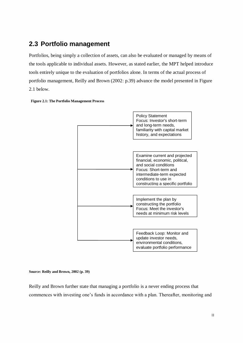
portfolio management, Reilly and Brown (2002: p.39) advance the model presented in Figure

2.1 below.

Source: Reilly and Brown, 2002 (p. 39)

Reilly and Brown further state that managing a portfolio is a never ending process that

commences with investing one‟s funds in accordance with a plan. Thereafter, monitoring and

Policy Statement Focus: Investor's short-term and long-term needs, familiarity with capital market history, and expectations

Examine current and projected financial, economic, political, and social conditions Focus: Short-term and intermediate-term expected conditions to use in constructing a specific portfolio

Implement the plan by constructing the portfolio Focus: Meet the investor's needs at minimum risk levels

Feedback Loop: Monitor and update investor needs, environmental conditions, evaluate portfolio performance

Figure 2.1: The Portfolio Management Process

12

updating the portfolio to reflect changes in investor needs, as dictated by the economy at

large, are necessary next steps.

Figure 2.1 points out that a policy statement is the first step in formal portfolio management

practice. The policy statement is likened to a blueprint that outlines the investor‟s goals,

preferences, constraints, and risk appetite explicitly. Upon analysing the investor‟s goals and

other factors contained within the policy statement, an investment strategy that suits the

statement can then be developed. The economic situation must of necessity be considered

alongside the client‟s wishes, as mirrored by the policy statement, in order to ensure that the

strategy reflects reality. Strategy development then gives way to portfolio construction. This

is a critical step in the process because some level of skill is required in coming up with a

portfolio that truly reflects the investor‟s risk appetite. Whilst small-scale individual investors

might simply make recourse to experience, intuition, or gut feelings when picking assets to

include in their portfolios, sophisticated investors often rely on more advanced tools. Perhaps

the foremost tool in this regard is mean-variance optimisation (MVO). According to Michaud

(2004), the goal of MVO is to find by quantitative means portfolios that optimally diversify

risk without reducing expected return. Going back to Reilly and Brown‟s model, the last step

enumerated is the continual monitoring of the portfolio. But how much monitoring is optimal?

Clearly, the step above, is somewhat contentious, and is one of the reasons why arguments for

and against active portfolio management exist.

In conclusion, when one considers the need to perform asset analysis as a step inherent within

investment strategy development, then portfolio or investment management can be said to

formally involve: the setting of an investment policy; the performance of asset analysis; the

construction of a portfolio; and the evaluation and revision of the portfolio when necessary.

2.4 Asset allocation

The process of asset allocation is synonymous with the portfolio construction step highlighted

above. It simply involves building a diversified portfolio by assigning weights to the different

asset classes that make up the portfolio. Indeed, it is a fact that, as Cardona (1998) asserts,

“different types of investments perform differently under various economic and political

13

scenarios”. Thus, this explains why diversification has become such an indispensible concept

in portfolio construction and therefore, why the need to have a diversified portfolio impacts

heavily on the asset allocation decision.

Before making a decision regarding the composition of a portfolio, Cardona (1998) opines

that four key factors should be considered, viz:

1. Objective: This refers to the investor‟s investment aim and personal financial goals.

2. Time horizon: This considers, among other issues, whether the investor‟s financial

goals would permit them sustain an extended decline in the market.

3. Risk vs. reward: This factor considers the investor‟s disposition to volatility or the

level of their risk aversion.

4. Financial situation: This considers how much of the investor‟s net worth is being

invested.

Upon considering the factors above, an investor should be better equipped to decide which

kinds of assets ought to be considered for investment and what allocation policy weights

should be assigned to the prospective assets. Thereafter, the specific assets to be included into

the portfolio can be determined by more precise analysis of individual assets coupled with the

broad guidelines developed from the considerations above.

Three key factors, obtainable from historical data, are typically considered when analysing

prospective assets identified for inclusion into a portfolio, viz:

1. Asset class returns

2. Asset class risk (standard deviation), and

3. Asset class correlation coefficients (the return relationship between two asset classes)

Once these inputs are calculated for each asset and used as inputs in a framework such as

MVO, the risk appetite of the investor would then help determine what weights to assign to

each asset within the portfolio.

14

2.4.1 Strategic asset allocation

Alongside tactical asset allocation, presented below, this is purportedly one of the most

popular forms of asset allocation. Cardona (1998) contends that this particular method is what

most investors think of when they hear the term asset allocation. In his words, it is the process

of “establishing weightings for different asset classes and rebalancing these holdings

periodically as the investor‟s overall personal and financial situation changes over time”.

However, the Institute of Business and Finance (IBF) defines this concept slightly differently

as the process of “designing a portfolio of investments that is suitable for your needs and

sticking with that allocation through all market conditions”.

2.4.2 Tactical asset allocation

This strategy, also referred to as market timing, is described as involving the process of

overweighting or underweighting different asset classes in order to improve returns. IBF

states that this strategy is dynamic and thus permits departures from a static asset allocation

based on some measure of market valuation.

2.5 Portfolio rebalancing

The self-explanatory phrase portfolio rebalancing refers to the process of resetting a portfolio

to its initial composition in terms of the weights allocated to the different assets. The need to

rebalance portfolios is borne out of the fact that the varying performances of the assets within

a portfolio guarantee that their weights will change over time. Donohue and Yip (2003: p.49)

put it this way:

As the proportions of wealth allocated to individual assets change due to

performance differences, changes in investor objectives or risk aversion, or the

introduction of new capital, investors must reallocate portfolio funds to bring

asset allocations back to given target ratios.

This means that, when portfolios are rebalanced, portions of assets that have performed really

well will be sold off and more units of poorly performing assets will be bought, in order to

bring all assets back to their policy or initial allocation weights.

15

2.5.1 Portfolio rebalancing example

Assume Table 2.1 below is the closing prices of stocks A, B, C and D over a 2-year period.

Table 2.1: Portfolio Rebalancing Example

Year Stock A (€) Stock B (€) Stock C (€) Stock D (€)

1 40 6 15 10

2 35 8 12 11

Assume further that 1€ was available to invest equally in all three stocks. This implies an

investment amount of or a weight of 25% for each stock. Investing in year 1

would mean that the following amount of shares will be bought for each stock:

In year 2, the initial investment of 1€ would have become the sum of the individual share

amounts multiplied by their closing prices in year 2:

This implies a return to the portfolio of 2.95% between year 1 and 2. However, as can be

expected, the assets will no longer have the same allocation weights of 25% they had in year

1. Going by the new portfolio value of 1.0295€, the stocks now have the following portfolio

weights:

16

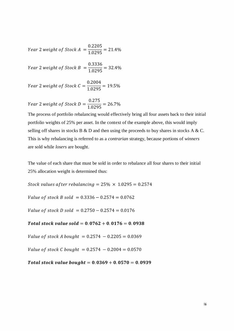
The process of portfolio rebalancing would effectively bring all four assets back to their initial

portfolio weights of 25% per asset. In the context of the example above, this would imply

selling off shares in stocks B & D and then using the proceeds to buy shares in stocks A & C.

This is why rebalancing is referred to as a contrarian strategy, because portions of winners

are sold while losers are bought.

The value of each share that must be sold in order to rebalance all four shares to their initial

25% allocation weight is determined thus:

17

The process above shows a simplified way of implementing the rebalancing process.

Typically, the value of shares sold from the portfolio should equate3 with the amount of new

shares purchased. The critical consideration is when exactly the asset weights should be

rebalanced.

2.5.2 Pros and cons of rebalancing

The primary goal and main benefit often associated with portfolio rebalancing is risk4

management. Si (2009) refers to this benefit as a certainty. This is because an investor that

chooses to rebalance clearly possesses the power to reset his portfolio to its allocation

weights, thus adjusting the portfolio risk to a desirable level. Portfolio returns, on the other

hand, whilst a possible benefit, is never certain. Another benefit adduced to rebalancing is the

buy-low/sell-high opportunity it avails investors. As was shown in the example above, when

stocks are rebalanced, high performers are sold and cheaper poor performers are bought

instead. Other advantages of portfolio management are more psychological in nature, and

involve the feeling of satisfaction and control that comes from seemingly being in control of

one‟s investment destiny by actively controlling a portfolio. Investors who rebalance also

have a feeling of discipline resulting from selling stocks even when they are doing well.

On the flipside, perhaps the most easily identifiable disadvantage of rebalancing, especially

compared to adopting a passive attitude to portfolio management is costs. Stock trading is

subject to direct and indirect costs and, ceteris paribus, the more one trades the higher these

costs. There are two main broad groupings of costs associated with trading shares and

rebalancing (by implication), as opined by Tokat (2006: p.10):

Fixed costs: This refers to time and labour costs and is typically charged by

investment managers and advisors for managing a client‟s portfolio. This is often a flat

one-off fee and is generally unrelated with the size of the trade.

Proportional costs: This category of costs vary with the size of the trade and refer to

taxes, redemption costs, fees, and bid-ask spreads. Hence, with these costs, the more a

portfolio is rebalanced the higher the associated proportional costs.

3 The difference of 0.0001 in the example is due to rounding errors. 4 It should be clear that only unsystematic risk can be managed by either diversification or rebalancing.

18

2.5.3 Rebalancing strategies

Rebalancing can be carried out in myriad ways, but the three main strategies, according to Si

(2009) and other authors are:

1. Periodic rebalancing: This simply refers to rebalancing portfolios according to

typical calendar intervals, such as monthly, quarterly, half-yearly, and annually.

2. Threshold rebalancing: This strategy can be interpreted and executed in two ways.

Firstly, portfolios are rebalanced when any asset grows or declines to a certain pre-

defined percentage, e.g. if an asset starts off with a weight of 5%, rebalancing could be

triggered with different predetermined percentages of say 10% for growth and 2% for

declines. On the other hand, rebalancing could be triggered if any asset deviates from

its initial allocation weight by one single pre-defined threshold percentage. For

example, a threshold percentage of ± 10% for growth or declines infers that an asset

with an initial weight of 5% would have to grow to 5.25% or decline to 4.75% in order

to trigger rebalancing.

3. Periodic monitoring: This method is a hybrid of the two strategies above. In this

case, the portfolio is monitored at calendar intervals like in the first strategy, and

action is only taken if a preset condition, like in the case of the second strategy, is met.

19

3 Review of previous studies

This chapter will cover a review of previous studies related to the subject matter. It is worth

stating that, a fair number of related studies were reviewed for this research, and quotes from

these studies feature prominently all over the paper. However, the decision to cover only four

studies in this chapter was made based on time constraints and the desire to provide depth

rather than breadth. More specifically, the studies reviewed were selected because of their

level of similarity with the approach used in this study.

The first of the four is of the behavioural finance genre, and will appropriately set the stage by

highlighting the benefits accruable from rebalancing. The other three all examine rebalancing

proper and will be examined chronologically. A concise summary of the findings from all

four studies will draw the curtains on this chapter.

3.1 Does Portfolio Rebalancing Help Investors Avoid

Common Mistakes?

In this study, Beach and Rose (2005) opine that the ability to accumulate wealth via investing

is inevitably impacted upon when individual investors and, strangely enough, professional

fund managers allow their emotions “get in the way of rational investment decision-making”.

While normal, these emotional responses are far from rational or, for that matter, optimal. The

authors point out that investors often enter or exit the market at the wrong time, and they

highlight three aspects of investment decision-making that are often responsible for this

phenomenon. At the heart of the study is an examination of the “impact of portfolio

rebalancing on reducing common investment mistakes and achieving investment goals”.

The three investment behaviour issues considered are Herd Mentality, Regret Aversion, and

Mental Accounting. Like the phrase implies, Herd Mentality refers to the tendency of

investors to do what is most popular at any given moment in time. Thus, investors are

sometimes wont to disregard good judgement and follow the crowd when deciding on what to

invest in. Regret Aversion refers to the desire for people to avoid facing up to the

consequences of bad decision making. As such, investors who make wrong bets and are

20

averse to feelings of regret, remain in denial and fail to cut their losses when they should. On

the flipside of this same phenomenon, investors who manage to cut their losses adopt the

“once beaten twice shy” maxim and stay away from investments that have “failed them”, even

when doing so is imprudent. Lastly, Mental Accounting describes the propensity of investors

to resort to rules-of-thumb during the asset allocation process. They often cite the complexity

involved in concepts like mean variance analysis as a reason why a subjective, and often

irrational approach, would suffice. Invariably, little regard is paid to the correlation between

assets in their portfolios and to the benefits that accrue from mixing assets with low

correlations.

3.1.1 Empirical Analysis

In order to point out the foolhardiness that typifies emotion-driven investing, twelve

“rebalancing” portfolios consisting of differing mixes of large-cap stocks, long-term bonds,

and T-bills were compared to a “Chase Portfolio”. The so-called Chase Portfolio is simply

synonymous to a momentum investment strategy wherein, during the current period , all

available investment funds are channelled into the asset class that pulled in the highest returns

over the previous period . The rebalanced portfolios were simply reset to their original

allocation weights annually.

Annual return data for the 77-year period 1926-2002 was used in the analysis. The twelve

rebalancing portfolios that were compared to the Chase portfolio contained weights varying

from 100% in stocks to 100% in long-term bonds, as shown in Table 3.1 below. A long-term

investment horizon was assumed, and T-Bills had a constant allocation of 5% in every

portfolio aside from the two at both extremes, which had 100% in stock and 100% in long-

term bonds respectively.

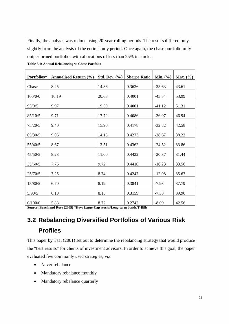
The results showed that the Chase portfolio had a lower Sharpe ratio than virtually all the

rebalanced portfolios. Thus, it did not generate enough returns to compensate for the risk

associated with holding such a portfolio. However, the Chase portfolio performed better than

portfolios with a stock allocation of less than 25%. The authors concluded that even the most

conservative investors are better off with an allocation of at least 45% in stocks, particularly

because the 45% portfolio had the highest Sharpe ratio.

21

Finally, the analysis was redone using 20-year rolling periods. The results differed only

slightly from the analysis of the entire study period. Once again, the chase portfolio only

outperformed portfolios with allocations of less than 25% in stocks.

Table 3.1: Annual Rebalancing vs Chase Portfolio

Portfolios* Annualised Return (%) Std. Dev. (%) Sharpe Ratio Min. (%) Max. (%)

Chase 8.25 14.36 0.3626 -35.63 43.61

100/0/0 10.19 20.63 0.4001 -43.34 53.99

95/0/5 9.97 19.59 0.4001 -41.12 51.31

85/10/5 9.71 17.72 0.4086 -36.97 46.94

75/20/5 9.40 15.90 0.4178 -32.82 42.58

65/30/5 9.06 14.15 0.4273 -28.67 38.22

55/40/5 8.67 12.51 0.4362 -24.52 33.86

45/50/5 8.23 11.00 0.4422 -20.37 31.44

35/60/5 7.76 9.72 0.4410 -16.23 33.56

25/70/5 7.25 8.74 0.4247 -12.08 35.67

15/80/5 6.70 8.19 0.3841 -7.93 37.79

5/90/5 6.10 8.15 0.3159 -7.38 39.90

0/100/0 5.88 8.72 0.2742 -8.09 42.56 Source: Beach and Rose (2005) *Key: Large-Cap stocks/Long-term bonds/T-Bills

3.2 Rebalancing Diversified Portfolios of Various Risk

Profiles

This paper by Tsai (2001) set out to determine the rebalancing strategy that would produce

the “best results” for clients of investment advisors. In order to achieve this goal, the paper

evaluated five commonly used strategies, viz:

Never rebalance

Mandatory rebalance monthly

Mandatory rebalance quarterly

22

Rebalance if any asset class drifts by more than five percentage points at month-end

Rebalance if any asset class drifts by more than five percentage points at quarter-end

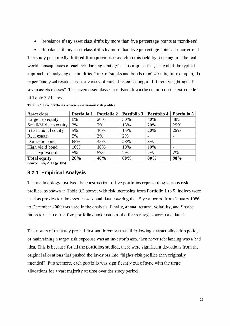
The study purportedly differed from previous research in this field by focusing on “the real-

world consequences of each rebalancing strategy”. This implies that, instead of the typical

approach of analysing a “simplified” mix of stocks and bonds (a 60-40 mix, for example), the

paper “analysed results across a variety of portfolios consisting of different weightings of

seven assets classes”. The seven asset classes are listed down the column on the extreme left

of Table 3.2 below.

Table 3.2: Five portfolios representing various risk profiles

Asset class Portfolio 1 Portfolio 2 Portfolio 3 Portfolio 4 Portfolio 5

Large cap equity 8% 20% 30% 40% 48%

Small/Mid cap equity 2% 7% 13% 20% 25%

International equity 5% 10% 15% 20% 25%

Real estate 5% 3% 2% - -

Domestic bond 65% 45% 28% 8% -

High yield bond 10% 10% 10% 10% -

Cash equivalent 5% 5% 2% 2% 2%

Total equity 20% 40% 60% 80% 98% Source:Tsai, 2001 (p. 105)

3.2.1 Empirical Analysis

The methodology involved the construction of five portfolios representing various risk

profiles, as shown in Table 3.2 above, with risk increasing from Portfolio 1 to 5. Indices were

used as proxies for the asset classes, and data covering the 15 year period from January 1986

to December 2000 was used in the analysis. Finally, annual returns, volatility, and Sharpe

ratios for each of the five portfolios under each of the five strategies were calculated.

The results of the study proved first and foremost that, if following a target allocation policy

or maintaining a target risk exposure was an investor‟s aim, then never rebalancing was a bad

idea. This is because for all the portfolios studied, there were significant deviations from the

original allocations that pushed the investors into “higher-risk profiles than originally

intended”. Furthermore, each portfolio was significantly out of sync with the target

allocations for a vast majority of time over the study period.

23

With regards to the four strategies, compared to the never rebalancing strategy, the study

showed that they produced “similar risks and returns”. The highest reported return differential

between any two of the strategies was 29 basis points and the lowest was 9 basis points, while

the risk differentials ranged from a low of 8 to a high of 36 basis points. In addition, the

author reports that no single strategy was optimal across all portfolios save for the never

rebalancing strategy that consistently had the lowest Sharpe ratio.

As a result of the arguably insignificant differences in risk-adjusted returns accruing from the

four strategies, the author concluded that advisors should consider other criteria when

determining what is most optimal. Examples of such criteria are “investors‟ sensitivity to

transaction frequency and taxes”, and to the advisor‟s own “programming and systems

limitations”. In the face of such considerations the “rebalance if any asset class drifts by more

than five percentage at month-end” strategy proved to be the somewhat better choice, because

it had the best Sharpe ratio of all the other strategies three times out of five and was never

worse than third best. Furthermore, over the 15 year period, this strategy only triggered

between four and ten transactions across all five portfolios.

3.3 The Benefits of Rebalancing

Buetow et al (2002) set out to demonstrate how pension funds and other tax-exempt plan

sponsors could benefit from the value-adding capabilities of rebalancing strategies. Their

study‟s objectives were addressed via the following two questions:

Does rebalancing a fund‟s asset class allocations to the strategic target weights make

sense?

If it does, what is the best rebalancing strategy?

The authors point out that plan sponsors typically adopt either a disciplined or haphazard

approach to rebalancing their portfolios, with some rebalancing when cash inflows or

outflows dictate action, and others basing their strategies on time or deviations (drifts) from

target allocations. They point out further that since most plan sponsors employ “sophisticated

24

mean-variance efficient optimization techniques”, and justifiably so5, an undisciplined or

haphazard approach makes light of the “care and deliberation” that go into making the asset

allocation decision.

In their opinion, the control of risk ought to be the primary criteria for evaluating alternative

rebalancing strategies. They assert that since a good rebalancing strategy should either keep

risk constant or reduce it, whilst also increasing returns, a risk-adjusted measure of returns

would be the best way to evaluate different strategies. In addition to risk-adjusted returns,

they opine that trading costs and the feasibility of implementing the rebalancing strategy are

also critical considerations.

The authors assert that whereas other studies either considered frequency rebalancing6 or

interval rebalancing7 exclusively, their approach distinguishes itself from its predecessors by

combining both. This implies that, for example, if a weight of 60% is assigned to equities and

the rebalancing interval is taken to be 10%, then the equity portion of the portfolio would be

reset to its initial allocation weight of 60% anytime it deviates by ± 6%. Furthermore, if the

portfolio is monitored on a monthly basis, combining this with the rebalancing interval of

10% above means that, the equity portion would be rebalanced if it is found to be ≤ 54% or ≥

66% at month end.

3.3.1 Empirical Analysis

The authors evaluated intervals ranging from 1% to 20% and monitoring frequencies of daily,

monthly, quarterly, and semi-annually. In their methodology, whenever the rebalancing

criteria were met by any one asset class, all the other assets in the portfolio were reset to

initial allocation weights as well. In order to achieve robustness with the study, the authors

first utilised Monte Carlo simulations (ten-year investment horizon) in evaluating the

5 Buetow et al, 2002 assert that studies such as Brinson et al, 1986 and Ibbotson and Kaplan, 2000 point out that

the target asset allocation may be the most important aspect in explaining portfolio performance. 6 The authors define Frequency rebalancing as rebalancing on certain dates such as each month, each quarter, or

each year-end. 7 Interval rebalancing refers to instances where rebalancing is triggered by drifts in asset class allocations, such as

changes of 2%, 5%, or 10% from target weights.

25

rebalancing strategies and then followed this up by running tests using actual historical data

(daily return data from January, 1987 to August, 2000).

Table 3.3: Average Asset Exposures at Different Rebalancing Intervals

Average Asset Exposures at Different Rebalancing Intervals Using Daily Simulations

1% 5% 10% 20%

Correlation Equity Bonds Equity Bonds Equity Bonds Equity Bonds

-1.0 60.01% 39.99% 60.11% 39.89% 60.41% 39.59% 61.60% 38.40%

-0.5 60.01% 39.99% 60.13% 39.87% 60.52% 39.48% 62.01% 37.99%

0 60.01% 39.99% 60.17% 39.83% 60.67% 39.33% 62.44% 37.56%

0.5 60.01% 39.99% 60.24% 39.76% 60.84% 39.16% 63.13% 36.87%

1.0 60.02% 39.98% 60.42% 39.58% 61.47% 38.53% 64.09% 35.91%

Average Asset Exposures at Different Rebalancing Intervals Using Actual Daily Data

0.1462 60.07% 39.93% 61.02% 38.98% 62.33% 37.67% 64.76% 35.24% Source: Buetow et al, 2002 (p. 25)

Separate analyses were run for a two-asset portfolio case and a four-asset portfolio case

respectively. In the two-asset case, the S&P 500 index was used to proxy equities and the J.P.

Morgan All Government index was used to proxy bonds. The four-asset case, on the other

hand, consisted of U.S. large-cap and small-cap stocks, international stocks, and bonds. These

had the Russell 2000, EAFE8, and J.P. Morgan All Government indexes as proxies

respectively.

The base case for two-asset class analysis was a traditional 60/40 mix of equities and bonds.

The Monte Carlo simulations were carried out utilising equity-bond correlations of -1.0, -0.5,

0, 0.5, and 1.0. The results showed that as the intervals increased from 1% to 20%, the

average weightings in equities also increased expectedly. This phenomenon known as equity

drift arises because equities typically perform better than bonds. This outcome was also

corroborated by the empirical analysis using actual data, as shown in Table 3.3 above. The

outcome of the analysis proved clearly that longer rebalancing frequencies exposed equities to

greater return prospects and, inevitably, greater risk. Furthermore, the results showed that the

benefits of a rebalancing strategy increased as asset correlation diminished. This led to the

observation that, just like with diversification, perfect negative correlation added the most

value in terms of rebalancing.

8 Europe, Australasia, Far East.

26

Table 3.4: Actual Net Returns and Risk Results for A 5% Rebalancing Interval (1987 – 2000)

Actual Net Returns and Risk Results for a 5% Rebalancing Interval (1987 – 2000)

Constant -Mix Daily Monthly Quarterly Semi-annual

Avg. Net Return (%) 13.46 13.81 12.32 12.30 12.22

Std. Dev. (%) 9.2 9.2 9.2 9.2 9.2

Return/Risk 1.46 1.50 1.34 1.34 1.33 Source: Buetow et al, 2002 (p. 25)

In order to place all strategies on the same footing, so as to facilitate sound comparisons, the

authors captured the average equity drift and adjusted the starting weights to equities. Thereby

ensuring that the average daily exposure for all the analysed rebalancing intervals were

approximately the same. When the strategies were compared after this adjustment, the results

showed that a 0%9 rebalancing interval produced the least favourable risk-adjusted return. In

comparison, merely increasing the interval to 5% resulted in very significant additional

returns. Beyond 5% the additional returns earned were rather slight. The authors thus

concluded that a rebalancing interval of 5% helped fulfil the strategic asset allocation

objective, whilst capturing most of the potential valued-added from rebalancing.

Monitoring frequencies were then evaluated to ascertain their impact on portfolio

performance. This phase of their study showed that monitoring the portfolio on a daily basis

and adjusting weights whenever the interval criterion (5%) was met produced better risk-

adjusted returns than monthly, quarterly, and semi-annual monitoring respectively. Table 3.4

above shows that the second best performer was the constant-mix portfolio, where the 60/40

mix was held constant throughout the analysis. There was very little difference between the

monthly, quarterly, and semi-annual frequencies. Hence, portfolio performance improved as

the monitoring frequency was shortened. Once again, as it was with the analysis of the

optimal interval, the results of the simulations and back testing using actual data were very

similar.

In the analysis of four asset classes, the most noteworthy conclusion was the assertion that,

according to the authors, “the potential returns increase slightly as the number of asset classes

increases”. Thus, they opine further, “dividing U.S. equities exposures into separate asset

9 This implies that the portfolio is held at target weights at all times.

27

classes such as large- and small-cap does increase the potential return and the consistency of

the strategy”. Invariably, the authors are of the opinion that the more disaggregated the

components of a portfolio, the better the benefits from rebalancing.

3.4 Alternative Portfolio Rebalancing Strategies Applied to

Sector Funds

Eakins and Stansell‟s (2007) study evaluates typical rebalancing strategies such as:

rebalancing at regular intervals of time and rebalancing “based on waiting until a particular

type of security grows to some threshold that triggers action”. As can be gleaned from the title

of their article, the focus of their analysis was on sector funds. Sector funds were selected

because the authors were of the opinion that they are “a relatively recent innovation in

investing”.

Their approach involved first comparing various threshold triggers to see which was most

optimal, and then comparing the selected threshold to rebalancing based on the following

intervals of time: monthly, quarterly, semi-annual, and annual.

3.4.1 Empirical Analysis

The analysis was performed on a sample of 19 sector funds, with monthly data covering the

7-year period from 1995 – 2001. The authors noted the fact that the internet sector was an

outlier with an annualised return of 42.1%, well above all other sectors. Thus, they saw the

need to perform the analysis first with the internet sector included and, in order to eliminate

bias, also without the internet sector.

At the start of the analysis, equal weights were given to all 19 sectors within the portfolio.

This resulted in an allocation of 5.26% each. Thereafter, various threshold percentages were

tried as triggers, and 9% was selected as the most optimal. On average, the “annualised return

was 3.676% higher when rebalancing occurred when any sector‟s fund rose to 9% of its

portfolio‟s total value than if there was no rebalancing”. The 9% threshold also resulted in the

highest Sharpe‟s ratio, although this was only marginally higher than the 8% and 10%

28

thresholds. In addition, the 9% trigger required only 9 rebalances over the 7-year study

period.

When the 9% threshold rebalancing strategy was compared to strategies involving time

intervals, it outperformed all but the annual rebalancing strategy. The authors identified

reducing exposure to the internet sector via rebalancing, during the market decline of the year

2000, as the main source of the returns enjoyed by the 9% and annual rebalancing strategies.

Without the internet sector, no gains came from rebalancing based on any of the analysed

strategies. Also, when the analysis was performed over a ten-year horizon10

, rebalancing

based on a threshold trigger proved to be better than annual rebalancing.

The authors concluded that “rebalancing reduced investor exposure to sectors that have grown

rapidly and may experience reduced performance”, and the specific rebalancing strategy

adopted was not as important as a disciplined and consistent rebalancing regime.

3.5 Literature review summary

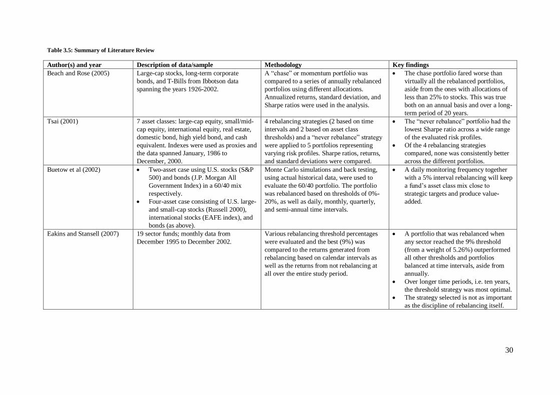
Beyond doubt, the studies reviewed in the preceding sub-chapters all proved, empirically, that

rebalancing has tangible merits. As a result, all the reviewed authors concluded that

disciplined rebalancing will not only help investors stay within their risk brackets, but also

has the potential of improving their portfolios‟ return generating potential. Unfortunately

however, this conclusion is where the similarities end as all four studies reached somewhat

unique conclusions. The main conclusions reached in four studies are given below, and

snapshots of the papers are presented in Table 3.5.

Beach and Rose (2005) concluded from their empirical analysis of annual rebalancing that an

allocation of 45% to equities would enhance the impact of rebalancing, whilst an allocation of

25% and below would militate against the benefits of rebalancing.

Tsai (2001), on the other hand, found that there were insignificant differences in the benefits

from rebalancing at monthly or quarterly time intervals, as well as from strategies involving a

10 The data set comprised of four funds with historical returns between 1992 and 2001

29

mix of a 5% asset drift alongside monthly and quarterly monitoring time intervals. This led to

the assertion that other considerations such as tax/transaction concerns or programming

limitations should be given pre-eminence in choosing a rebalancing strategy.

Buetow et al (2002) utilised Monte Carlo simulations and analysis of actual historical data to

determine that a hybrid strategy of daily monitoring and the use of a 5% asset drift threshold

was the most optimal with or without considering transaction costs. They thus concluded that

very frequent monitoring was beneficial, only if action on rebalancing was taken based on a

predetermined criterion, 5% in the case of their analysis.

Finally, Eakins and Stansell (2007) concluded from their own study that a 9% threshold for

rebalancing was the most optimal strategy. Considering that all the assets in their study started

with an allocation of 5.26%, this implied rebalancing only when any asset class, or sector

fund in the case of their study, grew or fell by about 71% or more than its initial allocation

weight.

30

Table 3.5: Summary of Literature Review

Author(s) and year Description of data/sample Methodology Key findings

Beach and Rose (2005) Large-cap stocks, long-term corporate

bonds, and T-Bills from Ibbotson data

spanning the years 1926-2002.

A “chase” or momentum portfolio was

compared to a series of annually rebalanced

portfolios using different allocations.

Annualized returns, standard deviation, and

Sharpe ratios were used in the analysis.

The chase portfolio fared worse than

virtually all the rebalanced portfolios,

aside from the ones with allocations of

less than 25% to stocks. This was true

both on an annual basis and over a long-

term period of 20 years.

Tsai (2001) 7 asset classes: large-cap equity, small/mid-

cap equity, international equity, real estate,

domestic bond, high yield bond, and cash

equivalent. Indexes were used as proxies and

the data spanned January, 1986 to

December, 2000.

4 rebalancing strategies (2 based on time

intervals and 2 based on asset class

thresholds) and a “never rebalance” strategy

were applied to 5 portfolios representing

varying risk profiles. Sharpe ratios, returns,

and standard deviations were compared.

The “never rebalance” portfolio had the

lowest Sharpe ratio across a wide range

of the evaluated risk profiles.

Of the 4 rebalancing strategies

compared, none was consistently better

across the different portfolios.

Buetow et al (2002) Two-asset case using U.S. stocks (S&P

500) and bonds (J.P. Morgan All

Government Index) in a 60/40 mix

respectively.

Four-asset case consisting of U.S. large-

and small-cap stocks (Russell 2000),

international stocks (EAFE index), and

bonds (as above).

Monte Carlo simulations and back testing,

using actual historical data, were used to

evaluate the 60/40 portfolio. The portfolio

was rebalanced based on thresholds of 0%-

20%, as well as daily, monthly, quarterly,

and semi-annual time intervals.

A daily monitoring frequency together

with a 5% interval rebalancing will keep

a fund‟s asset class mix close to

strategic targets and produce value-

added.

Eakins and Stansell (2007) 19 sector funds; monthly data from

December 1995 to December 2002.

Various rebalancing threshold percentages

were evaluated and the best (9%) was

compared to the returns generated from

rebalancing based on calendar intervals as

well as the returns from not rebalancing at

all over the entire study period.

A portfolio that was rebalanced when

any sector reached the 9% threshold

(from a weight of 5.26%) outperformed

all other thresholds and portfolios

balanced at time intervals, aside from

annually.

Over longer time periods, i.e. ten years,

the threshold strategy was most optimal.

The strategy selected is not as important

as the discipline of rebalancing itself.

31

4 Data and Research Methodology

4.1 Description of Data

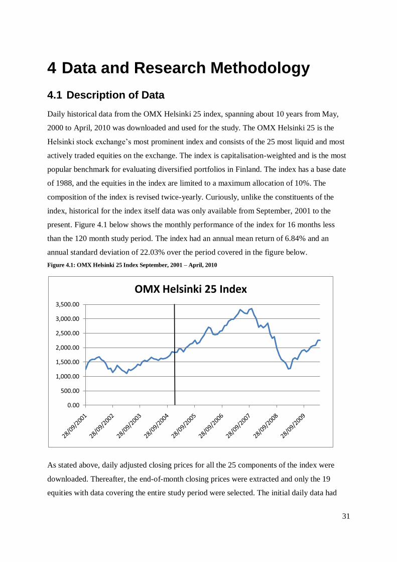
Daily historical data from the OMX Helsinki 25 index, spanning about 10 years from May,

2000 to April, 2010 was downloaded and used for the study. The OMX Helsinki 25 is the

Helsinki stock exchange‟s most prominent index and consists of the 25 most liquid and most

actively traded equities on the exchange. The index is capitalisation-weighted and is the most

popular benchmark for evaluating diversified portfolios in Finland. The index has a base date

of 1988, and the equities in the index are limited to a maximum allocation of 10%. The

composition of the index is revised twice-yearly. Curiously, unlike the constituents of the

index, historical for the index itself data was only available from September, 2001 to the

present. Figure 4.1 below shows the monthly performance of the index for 16 months less

than the 120 month study period. The index had an annual mean return of 6.84% and an

annual standard deviation of 22.03% over the period covered in the figure below.

Figure 4.1: OMX Helsinki 25 Index September, 2001 – April, 2010

As stated above, daily adjusted closing prices for all the 25 components of the index were

downloaded. Thereafter, the end-of-month closing prices were extracted and only the 19

equities with data covering the entire study period were selected. The initial daily data had

0.00

500.00

1,000.00

1,500.00

2,000.00

2,500.00

3,000.00

3,500.00

OMX Helsinki 25 Index

32

2499 data points and when divided by 250 business days results in approximately 9.99 years.

This was whittled down to 120 monthly data points spanning 31/05/2000 to 30/04/2010. In

order to generate statistics about the equities, the monthly closing prices were used to

calculate monthly returns by using Equation 4.1:

Equation 4.1: Return Calculated from Asset Closing Prices

Where refers to the closing price in a current month and refers to the closing price in

the preceding period. Thus, 119 return data points were subsequently obtained from the data.

Descriptive statistics of the 19 selected equities are presented in Table 4.1 below. The highest

average annual return, over the study period, of 17.58% was posted by YIT and the lowest

average annual return was Nokia‟s -18.23%. The table of correlations in Appendix A

indicates that the highest correlation coefficient of 0.88 was between Stora Enso and UPM-

Kymmene. This was totally expected, as both companies are in the wood pulp and paper

industry. The lowest correlation of 0.09, on the other hand, was between Sampo Bank and

Kone Cranes. The average correlation was quite low, and stood at 0.29.

4.2 Assumptions

The key assumptions used in the analysis are as follows:

1. It was assumed that at any rebalancing interval, stocks could be purchased at the

prevailing closing prices. Hence, no consideration was given to bid-ask spreads.

2. It was also assumed that all sales and purchase of stocks required to execute a

rebalancing strategy were carried out on the same day.

3. The analysis was performed without explicitly considering taxes and other transaction

costs.

33

4.3 Research Method

The method employed in carrying out the analysis involved the creation of spreadsheet

models for the different rebalancing strategies covered. First, a base case scenario was

considered. This involved the creation of an equally-weighted portfolio of all the 19

Table 4.1: Descriptive statistics of research data

Equity/Asset Name Mean

Mthly

Return

Mthly

Std Dev

Mean

Annual

Return

Annual

Std Dev

Min

Mthly

Return

Max

Mthly

Return

Elisa -0.74% 11.78% -8.92% 40.81% -56.48% 31.61%

Fortum 1.33% 7.67% 15.96% 26.57% -24.38% 20.97%

Kemira 0.49% 10.46% 5.86% 36.24% -43.82% 28.04%

Kesko 0.84% 8.62% 10.10% 29.87% -29.72% 24.88%

Konecranes -0.23% 15.47% -2.71% 53.58% -131.33% 21.04%

Metso 0.62% 12.09% 7.43% 41.87% -49.94% 27.52%

Nokia -1.52% 12.63% -18.23% 43.75% -42.96% 31.54%

Nokian Renkaat -0.52% 24.38% -6.25% 84.44% -225.85% 31.23%

Nordea Bank AB 0.04% 9.08% 0.51% 31.46% -26.08% 41.91%

Outokumpu 0.28% 11.51% 3.32% 39.88% -39.52% 33.35%

Pohjola Pankki A -0.22% 11.45% -2.59% 39.66% -72.79% 24.74%

Rautaruukki 0.90% 10.68% 10.75% 36.99% -51.38% 25.95%

Sampo A -0.74% 16.05% -8.94% 55.58% -152.09% 24.66%

Sanoma -0.05% 7.50% -0.61% 25.97% -18.19% 20.29%

Stora Enso R -0.40% 10.81% -4.74% 37.43% -36.75% 49.04%

Tieto -0.83% 12.84% -9.91% 44.47% -37.69% 32.01%

UPM-Kymmene -0.19% 9.85% -2.27% 34.11% -27.69% 45.11%

Wärtsilä 0.57% 12.27% 6.89% 42.51% -50.95% 46.27%

YIT 1.47% 11.04% 17.58% 38.26% -40.48% 36.57%

Equal weighted Portfolio 0.06% 6.66% 0.70% 23.08% -21.12% 26.01%

equities. Thus, each stock was attributed with a weight of or 5.26%. Since all

the portfolio weights must sum up to one (100%), this implied an investment of 1€ at the start

of the study period. This base case equally-weighted portfolio was not rebalanced at all over

the entire study period.

Again, considering the 5.26% weight assigned to each equity and the implied investment

value of 1€ above, this also meant that there was 0.0526€ available to invest on each asset.

The number of shares of each asset purchased at the start of the study period was determined

by dividing the investment amount by the prevailing closing price of each stock. For example,

34

the closing price of Elisa shares on 31/05/2000, the start of the study period, was 34.99€. This

implied that a total of shares of Elisa stock were purchased. In the

case of the no rebalancing base case portfolio, this number of Elisa shares would remain

unchanged for the entire 10-year study period. At the end of the study period, the value of the

portfolio was determined by multiplying the number of shares of each stock owned by the

prevailing closing price.

Thereafter, the same equally-weighted portfolio was analysed in spreadsheets that modelled

the three different rebalancing strategies introduced in Chapter 1; i.e., rebalancing based on

calendar intervals, rebalancing based on equity weight drift triggers, and a hybrid of both the

latter and the former strategies.

4.3.1 Rebalancing based on calendar intervals

Under this strategy, four calendar intervals were considered, viz; monthly, quarterly, half-

yearly, and annually. The start point of the analysis was the equally-weighted portfolio, and

the strategy involved resetting the assets in the portfolio to their initial allocation weights of

5.26% at the end of every time period. Using the annual strategy as an example, at year end

the resulting portfolio value was again split into 19 equal parts (5.26% each of the resulting

portfolio value). This was achieved by selling the part of any equity that exceeded its initial

5.26% allocation, and buying more shares to shore up stocks whose portfolio proportions

were below their initial allocation weights.

4.3.2 Rebalancing based on initial allocation weight drifts

In this strategy, which implies constant monitoring of the portfolio, predetermined drift

percentages were used to determine when rebalancing was required. Commencing with the

initial 5.26% allocation weights if, for example in the case of a 10% drift trigger, any asset

grew or declined by (i.e. approximately ± 53 basis points) all the assets in the

portfolio were reset to their initial allocation weights.

The percentage triggers used in the analysis ranged from 10% (± 53 basis points) to 100% (±

526 basis points), with 10% intervals. In the case of the 100% trigger, it implied that

rebalancing was only done if any asset attained a weight that was double its initial allocation

(i.e. 10.52%).

35

4.3.3 Rebalancing based a hybrid of calendar and weight drifts strategies

Here, a predetermined percentage drift trigger was utilised and action was only taken if any of

the stocks in the portfolio had fulfilled the trigger precondition during the monitoring interval.

In this case, unlike the preceding strategy, the portfolio was monitored at preset calendar

intervals (monthly, quarterly, half-yearly, and annually) to see if the rebalancing trigger

precondition was fulfilled.

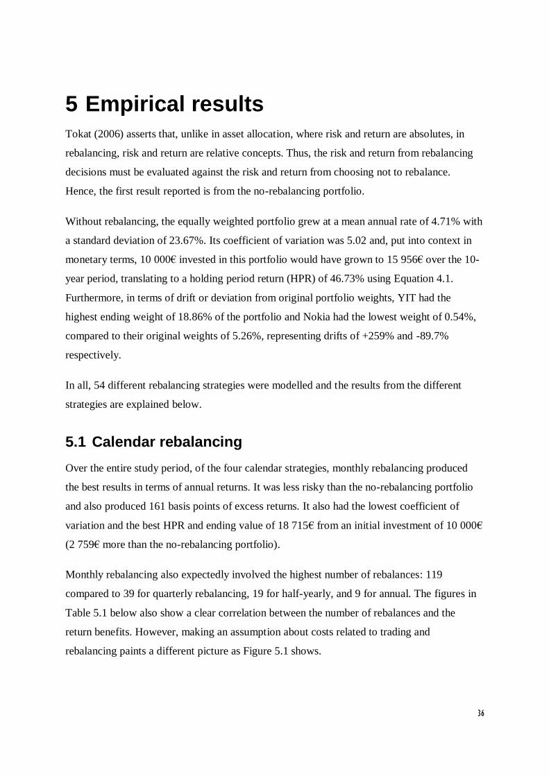
36

5 Empirical results

Tokat (2006) asserts that, unlike in asset allocation, where risk and return are absolutes, in

rebalancing, risk and return are relative concepts. Thus, the risk and return from rebalancing

decisions must be evaluated against the risk and return from choosing not to rebalance.

Hence, the first result reported is from the no-rebalancing portfolio.

Without rebalancing, the equally weighted portfolio grew at a mean annual rate of 4.71% with

a standard deviation of 23.67%. Its coefficient of variation was 5.02 and, put into context in

monetary terms, 10 000€ invested in this portfolio would have grown to 15 956€ over the 10-

year period, translating to a holding period return (HPR) of 46.73% using Equation 4.1.

Furthermore, in terms of drift or deviation from original portfolio weights, YIT had the

highest ending weight of 18.86% of the portfolio and Nokia had the lowest weight of 0.54%,

compared to their original weights of 5.26%, representing drifts of +259% and -89.7%

respectively.

In all, 54 different rebalancing strategies were modelled and the results from the different

strategies are explained below.

5.1 Calendar rebalancing

Over the entire study period, of the four calendar strategies, monthly rebalancing produced

the best results in terms of annual returns. It was less risky than the no-rebalancing portfolio

and also produced 161 basis points of excess returns. It also had the lowest coefficient of

variation and the best HPR and ending value of 18 715€ from an initial investment of 10 000€

(2 759€ more than the no-rebalancing portfolio).

Monthly rebalancing also expectedly involved the highest number of rebalances: 119

compared to 39 for quarterly rebalancing, 19 for half-yearly, and 9 for annual. The figures in

Table 5.1 below also show a clear correlation between the number of rebalances and the

return benefits. However, making an assumption about costs related to trading and

rebalancing paints a different picture as Figure 5.1 shows.

37

Assuming a cost range of 1 – 12 basis points, subject to the number of rebalances, e.g. a 1

basis point fee for each rebalance off the mean annual return translates to 1.19% less than the

original return. In this case, the 6.32% return to monthly rebalancing would reduce to 5.13%

per annum.

Table 5.1: Calendar Rebalancing Strategy

Calendar Freq

Ending Value

HPR Mean Annual R

Annual SD

CV # of Rebalances

# of -ve Months

# of +ve Months

Annual 1.5523 43.97% 4.43% 21.81% 4.92 9 54 65

Half-yearly 1.7243 54.48% 5.49% 21.80% 3.97 19 54 65

Quarterly 1.8463 61.32% 6.18% 21.88% 3.54 39 53 66

Monthly 1.8715 62.67% 6.32% 22.26% 3.52 119 54 65

Average 1.7481 55.58% 5.60% 22.44% 4.10 47 53 66

No-rebalancing

1.5956 46.73% 4.71% 23.67% 5.02 0 50 69

With the cost scenario shown below, annual and half-yearly rebalancing both become better

choices than the quarterly and monthly strategies from about 6 basis points and beyond. It is

also worth noting that beyond 4 basis points per rebalance in annual terms, no strategy would

beat the no-rebalancing portfolio (black horizontal line) returns-wise.

Figure 5.1: Cost Implication of Calendar Rebalancing

-7.00%

-5.00%

-3.00%

-1.00%

1.00%

3.00%

5.00%

7.00%

Mea

n A

nn

ual

Ret

urn

Cost per Rebalance

Annual

Half-yearly

Quarterly

Monthly

No Rebalancing

38

5.2 Percentage threshold rebalancing

The 10 strategies analysed under this category produced mixed results. The 50% threshold

had the best mean annual return of 6.43% per annum with the best HPR and portfolio ending

values of 63.81% and 18 929€ respectively. However, in terms of coefficient of variation, the

60% threshold with 12 rebalances had the best performance. From the 70% threshold and

below, considerately better returns were achieved compared to the no-rebalancing portfolio.

Above 70%, only the 90% trigger fared better than the no-rebalancing strategy. The

relationship between the number of rebalances and return generated was not as clear as it was

with the calendar strategy.

Table 5.2: Percentage Trigger Rebalancing Strategy

% Trigger Ending Value

HPR Mean Annual R

Annual SD

CV # of Rebalances

# of -ve Months

# of +ve Months

100% 1.5528 44.01% 4.44% 22.00% 4.96 3 53 66

90% 1.7425 55.53% 5.60% 21.73% 3.88 4 53 66

80% 1.5882 46.26% 4.67% 21.89% 4.69 4 52 67

70% 1.8273 60.29% 6.08% 21.58% 3.55 9 54 65

60% 1.8800 63.13% 6.37% 21.56% 3.39 12 53 66

50% 1.8929 63.81% 6.43% 21.99% 3.42 17 54 65

40% 1.8125 59.47% 6.00% 22.17% 3.70 22 53 66

30% 1.8851 63.40% 6.39% 22.01% 3.44 34 53 66

20% 1.8763 62.93% 6.35% 22.21% 3.50 56 53 66

10% 1.8679 62.48% 6.30% 22.26% 3.53 107 54 65

Average 1.7926 58.13% 5.86% 21.94% 3.81 27 53 66

No-rebalancing

1.5956 46.73% 4.71% 23.67% 5.02 0 50 69

Once again, taking cost assumptions into consideration, a strategy with fewer rebalancing

gains ascendancy, as shown in Figure 5.3 below. The 90% trigger performs best, from about 9

basis points and beyond, closely followed by the 60% trigger. These two triggers also perform

better than the no-rebalancing portfolio even up to the maximum assumed cost of 12 basis

points, whereas the 10% trigger underperforms the no-rebalancing portfolio from 3 basis

points and beyond, and even turns negative from about 6 basis points onwards.

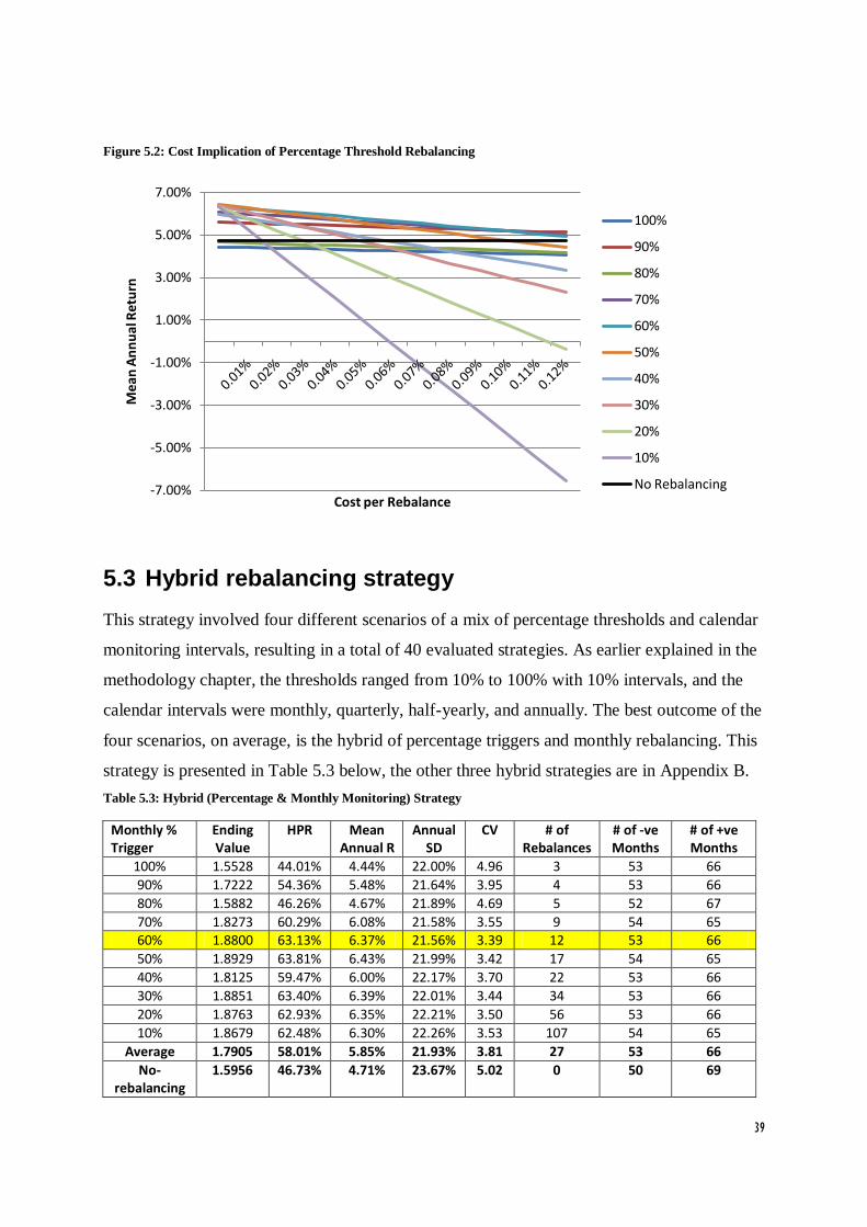
39

Figure 5.2: Cost Implication of Percentage Threshold Rebalancing

5.3 Hybrid rebalancing strategy

This strategy involved four different scenarios of a mix of percentage thresholds and calendar

monitoring intervals, resulting in a total of 40 evaluated strategies. As earlier explained in the

methodology chapter, the thresholds ranged from 10% to 100% with 10% intervals, and the

calendar intervals were monthly, quarterly, half-yearly, and annually. The best outcome of the

four scenarios, on average, is the hybrid of percentage triggers and monthly rebalancing. This

strategy is presented in Table 5.3 below, the other three hybrid strategies are in Appendix B.

Table 5.3: Hybrid (Percentage & Monthly Monitoring) Strategy

Monthly % Trigger

Ending Value

HPR Mean Annual R

Annual SD

CV # of Rebalances

# of -ve Months

# of +ve Months

100% 1.5528 44.01% 4.44% 22.00% 4.96 3 53 66

90% 1.7222 54.36% 5.48% 21.64% 3.95 4 53 66

80% 1.5882 46.26% 4.67% 21.89% 4.69 5 52 67

70% 1.8273 60.29% 6.08% 21.58% 3.55 9 54 65 60% 1.8800 63.13% 6.37% 21.56% 3.39 12 53 66

50% 1.8929 63.81% 6.43% 21.99% 3.42 17 54 65

40% 1.8125 59.47% 6.00% 22.17% 3.70 22 53 66

30% 1.8851 63.40% 6.39% 22.01% 3.44 34 53 66

20% 1.8763 62.93% 6.35% 22.21% 3.50 56 53 66

10% 1.8679 62.48% 6.30% 22.26% 3.53 107 54 65

Average 1.7905 58.01% 5.85% 21.93% 3.81 27 53 66

No-rebalancing

1.5956 46.73% 4.71% 23.67% 5.02 0 50 69

-7.00%

-5.00%

-3.00%

-1.00%

1.00%

3.00%

5.00%

7.00%

Me

an A

nn

ual

Re

turn

Cost per Rebalance

100%

90%

80%

70%

60%

50%

40%

30%

20%

10%

No Rebalancing

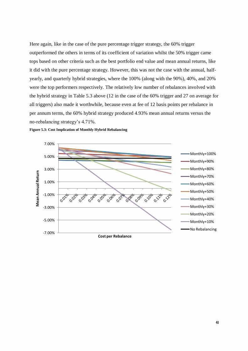
40

Here again, like in the case of the pure percentage trigger strategy, the 60% trigger

outperformed the others in terms of its coefficient of variation whilst the 50% trigger came

tops based on other criteria such as the best portfolio end value and mean annual returns, like

it did with the pure percentage strategy. However, this was not the case with the annual, half-

yearly, and quarterly hybrid strategies, where the 100% (along with the 90%), 40%, and 20%

were the top performers respectively. The relatively low number of rebalances involved with

the hybrid strategy in Table 5.3 above (12 in the case of the 60% trigger and 27 on average for

all triggers) also made it worthwhile, because even at fee of 12 basis points per rebalance in

per annum terms, the 60% hybrid strategy produced 4.93% mean annual returns versus the

no-rebalancing strategy‟s 4.71%.

Figure 5.3: Cost Implication of Monthly Hybrid Rebalancing

-7.00%

-5.00%

-3.00%

-1.00%

1.00%

3.00%

5.00%

7.00%

Mea

n A

nn

ual

Ret

urn

Cost per Rebalance

Monthly+100%

Monthly+90%

Monthly+80%

Monthly+70%

Monthly+60%

Monthly+50%

Monthly+40%

Monthly+30%

Monthly+20%

Monthly+10%

No Rebalancing

41

6 Conclusions and Recommendations

This paper set out to test different rebalancing strategies in order to determine which was

most optimal. It also set out to describe how investors can implement such a strategy. The

strategies were evaluated in terms of their annual returns and risk, as well as their coefficient

of variation and then compared to a no-rebalancing portfolio, as well as to one another. The

results of the analysis provided very convincing evidence to support the well accepted notion

that rebalancing enhances returns. This is because on average, the three main strategies

presented in the chapter above pulled in annual mean returns of 5.60%, 5.86%, and 5.85%,

compared to the no-rebalancing portfolio‟s annual mean return of 4.71%.

However, when proportional transaction costs are factored in, and calculated to reflect the

number of rebalances resulting from a particular strategy, very few outcomes are better than

the no-rebalancing portfolio. Also, the returns (and risk) differentials between different

strategies were rather slight – a maximum differential of 209 basis points between the best

and the worst strategies. This outcome is in tandem with one of the conclusions reached by

Tsai (2001) – “performance and risk differentials are small between the various strategies

tested”. That being said, considering the fact that it is only via rebalancing that assets within

portfolios can be kept in range of their allocation weight limits, the evidence from the analysis

proves clearly that particularly when costs are factored in, investors who choose to rebalance

their portfolios are better off applying strategies that result in as few instances of rebalancing

as possible.

If forced to select the most optimal of strategies, on the basis of the results obtained from the

analysis, ranking the results of all the 54 strategies would help to paint a clearer picture.

Appendices C and D contain tables where the results are ranked according to coefficient of

variation (CV) and holding period returns (HPR) respectively.

When ranked according to CV (Appendix C), the pure 60% strategy and the hybrid of 60%

with monthly monitoring led the 14 strategies in the upper quartile. Since the former involved

only 12 rebalances compared to the latter‟s 119, the pure 60% strategy is arguably the most

optimal based on ranking by CV. Of the 14 strategies in the upper quartile, 5 involve a hybrid

of monthly monitoring frequencies with triggers of 60%, 50%, 20%, & 10% respectively: 5

42

involve pure percentage strategies of 60%, 50%, 30%, 20%, & 10%: 2 involve a hybrid of

quarterly monitoring with 20% & 10% triggers: whilst monthly calendar rebalancing and

quarterly rebalancing had one instance each. The lower quartile was dominated by hybrids of

annual monitoring with percentage triggers (7 of the 14 strategies or 50%).

Appendix D presents the ranking by HPR. Here, the pure 50% strategy is joint top of the

upper percentile along with the hybrid of monthly monitoring and a 50% trigger. Once again,

one has to pick the former over the latter because of the fewer instances of rebalancing, 17

versus 119. The 14 strategies in the upper quartile as well as the 14 in the lower quartile also

mirror the ones highlighted in the previous paragraph.

In order not to draw conclusions based on what could very possibly have been mere

coincidence, the analysis was performed again using different time periods, so as to see which

strategies proved most consistent. Recall that the entire study period spanned 10 years from

31/05/2000 – 30/04/2010. In carrying out this second phase of the analysis, the data was split

into two halves of 5 years each. The first 5 years covered the period 31/05/2000-29/04/2005

whilst the second 5 years spanned 31/05/2005-30/04/2010. The vertical line in Figure 4.1

shows the division between the two time periods. The split data was then used in the analysis,

i.e., the 54 rebalancing strategies were analysed using each split data set exclusively. The

results from this analysis were subsequently ranked according to their coefficients of variation

and the strategies in the upper quartile11

were compared to see if there was any consistency

between the two time periods, as well as with the entire 10-year time period. The upper

quartiles for the two 5-year time periods and the 10-year study period are presented in

Appendix E.

A total of 25 different strategies showed up in the upper quartiles of the 3 time periods, as can

be seen in Table 6.1 below. Twelve of the strategies featured in the upper quartile of only one

time period, nine featured in two time periods, and four strategies showed up consistently in

the upper quartile of all three time periods. The numbers in Table 6.1 represent the rank of

each strategy within the upper quartile of each time period. For example, the 60% strategy

which proved to be the most optimal based on this evidence, was 12th best out of 14 over the

11 There were 14 strategies in each quartile.

43

5-year period 31/05/2000-29/04/2005; 1st over the 31/05/2005-30/04/2010 time period; and 1

st

over the entire 10-year study period.

Table 6.1: Rankings of the upper quartile strategies over 3 time periods

S/N Strategy 31/05/00-29/04/05 31/05/05-30/04/10 31/05/00-30/04/10

1 60% 12 1 1

2 50% 6 5 3 3 30% 5 12 5

4 Quarterly 7 10 14

5 Monthly + 60% - 2 2

6 20% 3 - 7

7 Monthly + 50% - 6 4

8 70% 9 3 -

9 10% 2 - 11 10 Monthly 4 - 9

11 Quarterly + 20% - 7 10

12 Monthly + 30% - 13 6

13 Quarterly + 10% - 11 13

14 90% 1 - -

15 Monthly + 70% - 4 -

16 40% 8 - - 17 Quarterly + 40% - 8 -

18 Monthly + 20% - - 8

19 Quarterly + 50% - 9 -

20 80% 10 - -

21 100% 11 - -

22 Monthly + 10% - - 12

23 Annual + 100% 13 - - 24 Annual + 90% 14 - -

25 Quarterly + 30% - 14 -

The inference to be drawn from the above is simple: In order to obtain the best results from

rebalancing, portfolios should be monitored frequently (preferably on a monthly basis) but

rebalancing should only be carried out when any one asset grows or falls by 50-60% of its

allocation weight. This requires a high level of discipline, as the frequency of monitoring

could tempt investors to take action even when the trigger precondition is not met. In the case

of this study, in percentage terms, considering that all the assets had an initial weight of

5.26%, this means rebalancing should be carried out when assets fall to 2.10-2.63% or rise to

7.89-8.42%. This upper limit is not too far from 9% recommended by Eakins and Stansell

(2007) in their own study.

In terms of implementation, institutional investors being well equipped to handle daily or

even hourly monitoring frequencies, would have no problems with monthly monitoring. In the

44

case of smaller investors, effective monthly or frequent monitoring is much more possible

now than it ever was. Most stock exchange websites avail investors the opportunity to create

profiles with their actual portfolio compositions, and these portfolios reflect asset values in

real-time. Alternatively, simple spreadsheet models can be used to monitor stock holdings and

asset weights. Asset closing prices can then be entered into the spreadsheet on a monthly basis

and used to determine prevailing asset weights, and whether or not rebalancing is required.

Finally, the results show beyond doubt that when markets are efficient and stock returns

follow a random path, most efforts (rebalancing in this case) aimed at producing excess

returns are very likely to be futile. Particularly because there are costs associated with these

actions. This then makes it all the more puzzling to understand why fees should be paid to

advisors for prescribing strategies such as portfolio rebalancing. Beyond reasonable doubt,

with specific regard to portfolio rebalancing, a strategy implemented by an individual investor

using simple spreadsheet models is as likely to succeed as it is to fail, in terms of producing

excess returns.

Regarding future research, perhaps the most attractive study would be as regards the actual

gathering of micro data showing how individual investors rebalance their portfolios and how

these portfolios fare compared to more sophisticated institutional investors who engage a

retinue of analysts to monitor their portfolios and utilise advanced modelling and optimisation

techniques. Secondly, because time constraints did not permit its inclusion in this report, the

analysis of a strategy incorporating the use of mean variance optimisation in determining

appropriate weights each time the portfolio is rebalanced would be worth considering. This is

because, if risk management is the most realisable objective of rebalancing, considering that

asset risk is dynamic, only the use of MVO can guarantee an appropriate portfolio risk level at

each rebalancing interval.

45

References

1. American Century Investments, Cutting Through Correlation, April, 2007, retrieved May 23,

2010

https://institutional.americancentury.com/institutional/pdf/quarterly_reviews/perspective_Cutt

ingCorrelation.pdf

2. Beach, S.L. and Rose, C.C., „Does Portfolio Rebalancing Help Investors Avoid Common

Mistakes?‟, Journal of Financial Planning, Vol. 18, Issue 5, 2005, pp. 56-61.

3. Benninga, S., Financial Modelling, 2nd revised edn, MIT Press, 2000.

4. Berk, J. and DeMarzo, P., Corporate Finance, Pearson Education, Inc., Boston, 2007.

5. Buetow, G. Jr., Sellers, R., Trotter, D., Hunt, E., and Whipple, W. Jr., „The Benefits of

Rebalancing‟, The Journal of Portfolio Management, Winter Issue, 2002, pp. 23-32.

6. Cardona, J.C., „The asset allocation decision‟, ABA Banking Journal, Vol. 90, Issue 2, 1998,

pp. 94-96.

7. Connolly, J. , „Advisors Prescribe Regular Portfolio Rebalancing‟, National Underwriter /

Life & Health Financial Services, Vol. 105, Issue 51, 2001, pp. 5-6.

8. Donohue, C. And Yip, K., „Optimal Portfolio Rebalancing With Transaction Costs‟, The

Journal of Portfolio Management, Summer, 2003, pp. 49-63.

9. Eakins, S.G. and Stansell, S., „An examination of alternative portfolio rebalancing strategies

applied to sector funds‟, Journal of Asset Management, Vol. 8, Issue 1, 2007, pp 1-9.

10. García-Herrero, A. and Terada-Hagiwara, A., „Do Asian Investors Rebalance Their Portfolios

and What are the Consequences?‟, Journal of Asian Economics, 18, 2007, pp. 195-216.

11. Grinblatt, M., and Titman, S., Financial Markets and Corporate Strategy. 2nd edn, McGraw-

Hill, New York, 2002.

12. Institute of Business and Finance, Certified Fund Specialist (study materials) Modules 1-6,

2009.

13. Liljeblom, E., Löflund, A., Krokfors, S., „The Benefits from International Diversification for

Nordic Investors, Journal of Banking & Finance, 21, 1997, pp. 469-490.

14. Masters, S.J., „Rebalancing: Establishing a Consistent Framework‟, The Journal of Portfolio

Management, Spring, 2003, pp. 52-57.

15. OMX Nordic Exchange, OMX Helsinki Local Indexes, accessed May 22, 2010

http://omxnordicexchange.com/products/indexes/OMX_indexes/OMXH_Local_Index/

46

16. Reilly, F.K. and Brown, K.C., Investment Analysis and Portfolio Management, 7th edn,

South-Western College Pub, 2002.

17. Richard O. Michaud, Why Mean-Variance Optimization Isn’t Useful for Investment

Management, New Frontier Newsletter January, 2004, retrieved 23 May, 2010

http://www.newfrontieradvisors.com/about/research/Articles/documents/WhyMVOptimizatio

nisntuseful.pdf

18. Sharpe, W.F., Alexander, G.J., and Bailey, J.V., Investments, 5th edn, Prentice Hall, Inc.,

New Jersey, 1995.

19. Tokat, Y, Vanguard Investment Counseling & Research, Portfolio Rebalancing in Theory and

Practice, 2006, retrieved, 20 May, 2010

https://institutional.vanguard.com/iip/pdf/ICRRebalancing.pdf

20. Tsai, C.S., „Rebalancing diversified portfolios of various risk profiles‟, Journal of Financial

Planning, Vol. 14, Issue 10, 2001, pp 104-110.

21. Yaqing, Si, Department of Statistics, Iowa State University: The Benefits of Portfolio

Rebalancing and How They Can be Achieved, February 27, 2009, retrieved May 23, 2010

<http://siyaqing.public.iastate.edu/research/2008/01s.pdf>

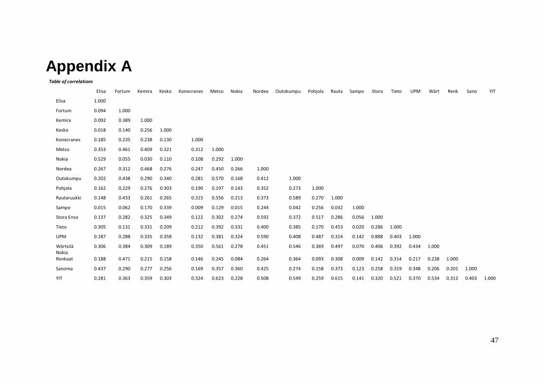
47

Appendix A Table of correlations

Elisa Fortum Kemira Kesko Konecranes Metso Nokia Nordea Outokumpu Pohjola Rauta Sampo Stora Tieto UPM Wärt Renk Sano YIT

Elisa 1.000

Fortum 0.094 1.000

Kemira 0.092 0.389 1.000

Kesko 0.018 0.140 0.256 1.000

Konecranes 0.185 0.235 0.238 0.130 1.000

Metso 0.353 0.461 0.409 0.321 0.312 1.000

Nokia 0.529 0.055 0.030 0.110 0.108 0.292 1.000

Nordea 0.267 0.312 0.468 0.276 0.247 0.450 0.266 1.000

Outokumpu 0.202 0.438 0.290 0.340 0.281 0.570 0.168 0.412 1.000

Pohjola 0.162 0.229 0.276 0.303 0.190 0.197 0.143 0.352 0.273 1.000

Rautaruukki 0.148 0.433 0.261 0.265 0.315 0.556 0.213 0.373 0.589 0.270 1.000

Sampo 0.015 0.062 0.170 0.339 0.009 0.129 0.015 0.244 0.042 0.256 0.032 1.000

Stora Enso 0.137 0.282 0.325 0.349 0.122 0.302 0.274 0.592 0.372 0.517 0.286 0.056 1.000

Tieto 0.305 0.131 0.331 0.209 0.212 0.392 0.331 0.400 0.385 0.170 0.453 0.020 0.286 1.000

UPM 0.187 0.288 0.335 0.358 0.132 0.381 0.324 0.590 0.408 0.487 0.314 0.142 0.888 0.403 1.000

Wärtsilä 0.306 0.384 0.309 0.189 0.350 0.561 0.278 0.451 0.546 0.369 0.497 0.070 0.406 0.392 0.434 1.000

Nokia Renkaat 0.188 0.471 0.215 0.158 0.146 0.245 0.084 0.264 0.364 0.093 0.308 0.009 0.142 0.314 0.217 0.238 1.000

Sanoma 0.437 0.290 0.277 0.256 0.169 0.357 0.360 0.425 0.274 0.158 0.373 0.123 0.258 0.319 0.348 0.206 0.201 1.000

YIT 0.281 0.363 0.359 0.303 0.324 0.623 0.228 0.508 0.549 0.259 0.615 0.141 0.320 0.521 0.370 0.534 0.312 0.403 1.000

48

Appendix B Annual % Trigger

Ending Value

HPR Mean Annual Return

Annual SD

CV # of Rebalances

# of -ve Months

# of +ve Months

100% 1.6531 50.27% 5.07% 22.17% 4.37 2 53 66

90% 1.6531 50.27% 5.07% 22.17% 4.37 2 53 66

80% 1.5964 46.77% 4.72% 21.78% 4.62 5 52 67

70% 1.5543 44.10% 4.45% 21.82% 4.91 5 54 65

60% 1.5543 44.10% 4.45% 21.82% 4.91 5 54 65

50% 1.5433 43.39% 4.38% 21.78% 4.98 6 53 66

40% 1.5523 43.97% 4.43% 21.81% 4.92 9 54 65

30% 1.5523 43.97% 4.43% 21.81% 4.92 9 54 65

20% 1.5523 43.97% 4.43% 21.81% 4.92 9 54 65

10% 1.5523 43.97% 4.43% 21.81% 4.92 9 54 65

Average 1.5764 45.48% 4.59% 21.88% 4.78 6 54 66

6 Months % Trigger

Ending Value

HPR Mean Annual Return

Annual SD

CV # of Rebalances

# of -ve Months

# of +ve Months

100% 1.6436 49.69% 5.01% 21.78% 4.35 3 54 65

90% 1.6651 50.99% 5.14% 22.17% 4.31 3 54 65

80% 1.5924 46.52% 4.69% 21.80% 4.65 5 52 67

70% 1.5543 44.10% 4.45% 21.82% 4.91 5 54 65

60% 1.5608 44.52% 4.49% 21.85% 4.87 6 54 65

50% 1.6462 49.85% 5.03% 21.81% 4.34 9 53 66

40% 1.7459 55.73% 5.62% 21.78% 3.88 15 54 65

30% 1.7431 55.57% 5.60% 21.81% 3.89 16 54 65

20% 1.7243 54.48% 5.49% 21.80% 3.97 19 54 65

10% 1.7243 54.48% 5.49% 21.80% 3.97 19 54 65

Average 1.6600 50.59% 5.10% 21.84% 4.31 10 54 65

Quarterly %Trigger

Ending Value

HPR Mean Annual Return

Annual SD

CV # of Rebalances

# of -ve Months

# of +ve Months

100% 1.6436 49.69% 5.01% 21.78% 4.35 3 54 65

90% 1.8313 60.50% 6.10% 21.79% 3.57 5 53 66

80% 1.7254 54.55% 5.50% 21.72% 3.95 7 53 66

70% 1.6331 49.05% 4.95% 21.72% 4.39 9 54 65

60% 1.6050 47.31% 4.77% 21.97% 4.61 10 53 66

50% 1.7359 55.15% 5.56% 21.84% 3.93 14 54 65

40% 1.7837 57.87% 5.84% 21.85% 3.74 20 54 65

30% 1.8153 59.62% 6.01% 21.94% 3.65 27 54 65

20% 1.8522 61.64% 6.22% 21.90% 3.52 38 53 66

10% 1.8463 61.32% 6.18% 21.88% 3.54 39 49 55

Average 1.7472 55.67% 5.61% 21.84% 3.92 17 53 64

49

Appendix C

Ranking by Coefficient of Variation Rank Strategy Ending

Value HPR Mean

Annual R Annual

SD CV # of

Rebalances

1 60% 1.8800 63.13% 6.37% 21.56% 3.39 12 2 Monthly + 60% 1.8800 63.13% 6.37% 21.56% 3.39 12 3 50% 1.8929 63.81% 6.43% 21.99% 3.42 17 4 Monthly + 50% 1.8929 63.81% 6.43% 21.99% 3.42 17

5 30% 1.8851 63.40% 6.39% 22.01% 3.44 34

6 Monthly + 30% 1.8851 63.40% 6.39% 22.01% 3.44 34 7 20% 1.8763 62.93% 6.35% 22.21% 3.50 56 8 Monthly + 20% 1.8763 62.93% 6.35% 22.21% 3.50 56 9 Monthly 1.8715 62.67% 6.32% 22.26% 3.52 119 10 Quarterly + 20% 1.8522 61.64% 6.22% 21.90% 3.52 38 11 10% 1.8679 62.48% 6.30% 22.26% 3.53 107 12 Monthly + 10% 1.8679 62.48% 6.30% 22.26% 3.53 107

13 Quarterly + 10% 1.8463 61.32% 6.18% 21.88% 3.54 39

14 Quarterly 1.8463 61.32% 6.18% 21.88% 3.54 39 15 70% 1.8273 60.29% 6.08% 21.58% 3.55 9 16 Monthly + 70% 1.8273 60.29% 6.08% 21.58% 3.55 9 17 Quarterly + 90% 1.8313 60.50% 6.10% 21.79% 3.57 5 18 Quarterly + 30% 1.8153 59.62% 6.01% 21.94% 3.65 27

19 40% 1.8125 59.47% 6.00% 22.17% 3.70 22 20 Monthly + 40% 1.8125 59.47% 6.00% 22.17% 3.70 22 21 Quarterly + 40% 1.7837 57.87% 5.84% 21.85% 3.74 20 22 6 months + 40% 1.7459 55.73% 5.62% 21.78% 3.88 15 23 90% 1.7425 55.53% 5.60% 21.73% 3.88 4

24 6 months + 30% 1.7431 55.57% 5.60% 21.81% 3.89 16 25 Quarterly + 50% 1.7359 55.15% 5.56% 21.84% 3.93 14

26 Monthly + 90% 1.7222 54.36% 5.48% 21.64% 3.95 4 27 Quarterly + 80% 1.7254 54.55% 5.50% 21.72% 3.95 7 28 6 months + 20% 1.7243 54.48% 5.49% 21.80% 3.97 19 29 6 months + 10% 1.7243 54.48% 5.49% 21.80% 3.97 19 30 Half-yearly 1.7243 54.48% 5.49% 21.80% 3.97 19 31 6 months + 90% 1.6651 50.99% 5.14% 22.17% 4.31 3

32 6 months + 50% 1.6462 49.85% 5.03% 21.81% 4.34 9 33 6 months + 100% 1.6436 49.69% 5.01% 21.78% 4.35 3 34 Quarterly + 100% 1.6436 49.69% 5.01% 21.78% 4.35 3 35 Annual + 100% 1.6531 50.27% 5.07% 22.17% 4.37 2 36 Annual + 90% 1.6531 50.27% 5.07% 22.17% 4.37 2 37 Quarterly + 70% 1.6331 49.05% 4.95% 21.72% 4.39 9 38 Quarterly + 60% 1.6050 47.31% 4.77% 21.97% 4.61 10

39 Annual + 80% 1.5964 46.77% 4.72% 21.78% 4.62 5 40 6 months + 80% 1.5924 46.52% 4.69% 21.80% 4.65 5 41 80% 1.5882 46.26% 4.67% 21.89% 4.69 4 42 Monthly + 80% 1.5882 46.26% 4.67% 21.89% 4.69 5 43 6 months + 60% 1.5608 44.52% 4.49% 21.85% 4.87 6 44 Annual + 70% 1.5543 44.10% 4.45% 21.82% 4.91 5

45 Annual + 60% 1.5543 44.10% 4.45% 21.82% 4.91 5 46 6 months + 70% 1.5543 44.10% 4.45% 21.82% 4.91 5 47 Annual + 40% 1.5523 43.97% 4.43% 21.81% 4.92 9 48 Annual + 30% 1.5523 43.97% 4.43% 21.81% 4.92 9 49 Annual + 20% 1.5523 43.97% 4.43% 21.81% 4.92 9 50 Annual + 10% 1.5523 43.97% 4.43% 21.81% 4.92 9

51 Annual 1.5523 43.97% 4.43% 21.81% 4.92 9 52 100% 1.5528 44.01% 4.44% 22.00% 4.96 3 53 Monthly + 100% 1.5528 44.01% 4.44% 22.00% 4.96 3 54 Annual + 50% 1.5433 43.39% 4.38% 21.78% 4.98 6

Q3

Q1

50

Appendix D

Ranking by HPR Rank Strategy Ending

Value HPR Mean

Annual R Annual

SD CV # of

Rebalances

1 50% 1.8929 63.81% 6.43% 21.99% 3.42 17 2 Monthly + 50% 1.8929 63.81% 6.43% 21.99% 3.42 17 3 30% 1.8851 63.40% 6.39% 22.01% 3.44 34 4 Monthly + 30% 1.8851 63.40% 6.39% 22.01% 3.44 34

5 60% 1.8800 63.13% 6.37% 21.56% 3.39 12 6 Monthly + 60% 1.8800 63.13% 6.37% 21.56% 3.39 12 7 20% 1.8763 62.93% 6.35% 22.21% 3.50 56 8 Monthly + 20% 1.8763 62.93% 6.35% 22.21% 3.50 56 9 Monthly 1.8715 62.67% 6.32% 22.26% 3.52 119 10 10% 1.8679 62.48% 6.30% 22.26% 3.53 107

11 Monthly + 10% 1.8679 62.48% 6.30% 22.26% 3.53 107 12 Quarterly + 20% 1.8522 61.64% 6.22% 21.90% 3.52 38 13 Quarterly + 10% 1.8463 61.32% 6.18% 21.88% 3.54 39 14 Quarterly 1.8463 61.32% 6.18% 21.88% 3.54 39 15 Quarterly + 90% 1.8313 60.50% 6.10% 21.79% 3.57 5 16 70% 1.8273 60.29% 6.08% 21.58% 3.55 9

17 Monthly + 70% 1.8273 60.29% 6.08% 21.58% 3.55 9 18 Quarterly + 30% 1.8153 59.62% 6.01% 21.94% 3.65 27 19 40% 1.8125 59.47% 6.00% 22.17% 3.70 22 20 Monthly + 40% 1.8125 59.47% 6.00% 22.17% 3.70 22 21 Quarterly + 40% 1.7837 57.87% 5.84% 21.85% 3.74 20 22 6 months + 40% 1.7459 55.73% 5.62% 21.78% 3.88 15

23 6 months + 30% 1.7431 55.57% 5.60% 21.81% 3.89 16 24 90% 1.7425 55.53% 5.60% 21.73% 3.88 4 25 Quarterly + 50% 1.7359 55.15% 5.56% 21.84% 3.93 14 26 Quarterly + 80% 1.7254 54.55% 5.50% 21.72% 3.95 7 27 6 months + 20% .7243 54.48% 5.49% 21.80% 3.97 19 28 6 months + 10% 1.7243 54.48% 5.49% 21.80% 3.97 19

29 Half-yearly 1.7243 54.48% 5.49% 21.80% 3.97 19 30 Monthly + 90% 1.7222 54.36% 5.48% 21.64% 3.95 4 31 6 months + 90% 1.6651 50.99% 5.14% 22.17% 4.31 3 32 Annual + 100% 1.6531 50.27% 5.07% 22.17% 4.37 2 33 Annual + 90% 1.6531 50.27% 5.07% 22.17% 4.37 2 34 6 months + 50% 1.6462 49.85% 5.03% 21.81% 4.34 9

35 6 months + 100% 1.6436 49.69% 5.01% 21.78% 4.35 3 36 Quarterly + 100% 1.6436 49.69% 5.01% 21.78% 4.35 3 37 Quarterly + 70% 1.6331 49.05% 4.95% 21.72% 4.39 9 38 Quarterly + 60% 1.6050 47.31% 4.77% 21.97% 4.61 10 39 Annual + 80% 1.5964 46.77% 4.72% 21.78% 4.62 5 40 6 months + 80% 1.5924 46.52% 4.69% 21.80% 4.65 5

41 80% 1.5882 46.26% 4.67% 21.89% 4.69 4 42 Monthly + 80% 1.5882 46.26% 4.67% 21.89% 4.69 5 43 6 months + 60% 1.5608 44.52% 4.49% 21.85% 4.87 6 44 Annual + 70% 1.5543 44.10% 4.45% 21.82% 4.91 5 45 Annual + 60% 1.5543 44.10% 4.45% 21.82% 4.91 5 46 6 months + 70% 1.5543 44.10% 4.45% 21.82% 4.91 5

47 100% 1.5528 44.01% 4.44% 22.00% 4.96 3 48 Monthly + 100% 1.5528 44.01% 4.44% 22.00% 4.96 3 49 Annual + 40% 1.5523 43.97% 4.43% 21.81% 4.92 9 50 Annual + 30% 1.5523 43.97% 4.43% 21.81% 4.92 9 51 Annual + 20% 1.5523 43.97% 4.43% 21.81% 4.92 9 52 Annual + 10% 1.5523 43.97% 4.43% 21.81% 4.92 9

53 Annual 1.5523 43.97% 4.43% 21.81% 4.92 9 54 Annual + 50% 1.5433 43.39% 4.38% 21.78% 4.98 9

Q1

Q3

51

Appendix E Upper Quartile Ranking by CV for three time periods

31/05/2000-29/04/2005 Rank Strategy Ending Value HPR Mean Annual R Annual SD CV # of Rebalances

No Rebalancing 1.2355 21.15% 4.30% 19.48% 4.53 0

1 90% 1.3034 26.49% 3.40% 18.44% 3.42 2

2 10% 1.3105 27.04% 5.50% 18.83% 3.42 53

3 20% 1.3101 27.01% 5.49% 18.82% 3.43 26

4 Monthly 1.3104 27.04% 5.50% 18.87% 3.43 58

5 30% 1.3028 26.45% 5.38% 18.89% 3.51 16

6 50% 1.2924 25.65% 5.22% 18.88% 3.62 8

7 Quarterly 1.2667 23.64% 4.81% 18.78% 3.91 19

8 40% 1.2668 23.65% 4.81% 18.92% 3.93 10

9 70% 1.2458 21.98% 4.47% 18.12% 4.05 3

10 80% 1.2463 22.02% 4.48% 18.34% 4.10 3

11 100% 1.2487 22.21% 4.52% 18.92% 4.19 1

12 60% 1.2401 21.52% 4.38% 18.52% 4.23 4

13 Annual + 100% 1.2273 20.48% 4.17% 18.76% 4.50 1

14 Annual + 90% 1.2273 20.48% 4.17% 18.76% 4.50 1

31/05/2005-30/04/2010 Rank Strategy Ending Value HPR Mean Annual R Annual SD CV # of Rebalances

No Rebalancing 1.1138 10.77% 2.19% 25.41% 11.60 0

1 60% 1.3948 33.28% 6.77% 24.12% 3.56 7

2 Monthly + 60% 1.3948 33.28% 6.77% 24.12% 3.56 7

3 70% 1.3606 30.79% 6.26% 24.48% 3.91 5

4 Monthly + 70% 1.3606 30.79% 6.26% 24.48% 3.91 5

5 50% 1.3521 30.17% 6.14% 24.65% 4.02 8

6 Monthly + 50% 1.3521 30.17% 6.14% 24.65% 4.02 8

7 Quarterly + 20% 1.3473 29.81% 6.06% 24.54% 4.05 18

8 Quarterly + 40% 1.3456 29.69% 6.04% 24.45% 4.05 9

9 Quarterly + 50% 1.3428 29.47% 5.99% 24.36% 4.06 7

10 Quarterly 1.3451 29.65% 6.03% 24.53% 4.07 19

11 Quarterly + 10% 1.3451 29.65% 6.03% 24.53% 4.07 19

12 30% 1.3412 29.36% 5.97% 24.67% 4.13 17

13 Monthly + 30% 1.3412 29.36% 5.97% 24.67% 4.13 17

14 Quarterly + 30% 1.3274 28.32% 5.76% 24.43% 4.24 10

Full study period 31/05/2000-30/04/2010 Rank Strategy Ending Value HPR Mean Annual R Annual SD CV # of Rebalances

No Rebalancing 1.5956 46.73% 4.71% 23.67% 5.02 0

1 60% 1.8800 63.13% 6.37% 21.56% 3.39 12

2 Monthly + 60% 1.8800 63.13% 6.37% 21.56% 3.39 119

3 50% 1.8929 63.81% 6.43% 21.99% 3.42 17

4 Monthly + 50% 1.8929 63.81% 6.43% 21.99% 3.42 119

5 30% 1.8851 63.40% 6.39% 22.01% 3.44 34

6 Monthly + 30% 1.8851 63.40% 6.39% 22.01% 3.44 119

7 20% 1.8763 62.93% 6.35% 22.21% 3.50 56

8 Monthly + 20% 1.8763 62.93% 6.35% 22.21% 3.50 119

9 Monthly 1.8715 62.67% 6.32% 22.26% 3.52 119

10 Quarterly + 20% 1.8522 61.64% 6.22% 21.90% 3.52 39

11 10% 1.8679 62.48% 6.30% 22.26% 3.53 107

12 Monthly + 10% 1.8679 62.48% 6.30% 22.26% 3.53 119

13 Quarterly + 10% 1.8463 61.32% 6.18% 21.88% 3.54 39

14 Quarterly 1.8463 61.32% 6.18% 21.88% 3.54 39