WORKING PAPER NO.272

Optimal Selection of Obsolescence Mitigation Strategi~ Using a Class of Bandit Models

By

Dinesh Kumar Haritha Saranga

May 2008

Please address all your correspondence to:

Prof. U. Dinesh Kumar Quantitative Methods & Infonnation Systems Indian Institute of Management Bangalore Bannerghatta Road Bangalore - 560 076 INDIA Email: dineshk@iimb.emetin Phone: 26993146(0)

Prof. Haritha Saranga Production & Operations Management Indian Institute of Management Bangalore Bannerghatta Road Bangalore - 560 076 INDIA Email: harithas@iimb.emetin Phone: 26993130(0)

Abstract

Optimal Selection of Obsolescence Mitigation Strategies Using a Class of Bandit Models

U Dinesh Kumarl and Haritha Saranga2

Indian Institute of Management Bangalore Bannerghatta Road, Bangalore 560076, INDIA

lEmail: dineshk@iimb.ernet.in 2Email: harithas@iimb.ernet.in

Obsolescence of embedded parts is a serious concern for managers of complex systems where

the design life of the system typically exceeds 20 years. Capital asset management teams have

been exploring several strategies to mitigate risks associated with Diminishing Manufacturing

Sources (DMS) and repeated life extensions of complex systems. Asset management cost and

the performance of a system depend heavily on the obsolescence mitigation strategy chosen by

the decision maker. We have developed mathematical models that can be used to calculate the

impact of various obsolescence mitigation strategies on the Total Cost of Ownership (TCO) of a

system. We have used classical multi-arm bandit (MAB), arm-acquiring bandit and restless

bandit models to jdentify the best strategy for managing obsolescence in such instances wherein

organizations have to deal with ~ontinuous technological evolution under uncertainty.

Keywords: Arm-acquiring bandit model, Gittins Index, Markov decision process, Multi-arm

bandit (MAB) model, obsolescence, Restless bandits (RB), total cost of ownership.

1.0 tntroduction

Technological innovation is no longer an option, but a necessity; indeed a vital survival

strategy for many companies, especially the electronic parts manufacturers. The advantages of

technological innovation are well documented in the literature (Capon et aI, 1992, Gatignon et

al 2002); Capon et al (1992), provide empirical evidence, based on a survey of 113

manufacturing firms selected from Fortune 500 manufacturers, that the firms that invest heavily

1

in innovation perfonn best financially. However, the main disadvantage of technological

innovation is the reduction in the economic life of parts as availability of better technology

renders the older technology less useful (Lee and Lee, 1988). Most complex systems, especially,

defence systems such as fighter aircraft, battle ships, tanks etc have long life, much longer than

many of their embedded parts. Managing such complex systems under continuous technological

changes has become a major challenge to many defence services and defence original equipment

manufacturers (OEMs). The main causes of part obsolescence are: (1) Diminishing

Manufacturing Sources (DMS) triggered by rapid progress in technology and (2) Life extension

of capital assets far beyond the life of its embedded parts, in particular, defence systems, and (3)

Planned obsolescence by many consumer durable manufacturers. Defence systems usually have

long design period (time spent on designing the product in the development life cycle), for

example, the design period for F-22 aircraft was more than 10 years and many parts of F-22

became obsolete even before the production started (Hitt and Schmidt, 1998). Boeing's B-52

Bomber project began in 1946 and the first flight took off in 1952. It is predicted that B-52

would still be flying for the US air force in 2045; almost a century after its development began

(Feltus, 2007). The projected electronic obsolescence budget for the F-22 fighter is in excess of

one billion dollars (Tepp, 1999).

Defence Supply Centre Columbus (DSCC) deals with procurement and quality assurance

of over 2.2 million spare parts and on an average 10,000 parts become obsolete every year

because of discontinuance of production by the manufacturer (Johnson, 2002). It is reported that

84% of the discontinued items are electronic components and the rest are mechanical and passive

devices (Tomczykowski, 2003). In 2005, more than 150,000 integrated circuits (lCs) were

declared end of life (Shott, 2006). Solomon et al (2000) claim that obsolescence of electronic

2

parts is a major reason for the high life cycle cost of military systems. The problem has become

a serious concern for product support managers of defence systems due to the rapid progress in

electronic technology wherein a new generation of components replace the old generation

components within months (Meyor et aI2004).

The impact of obsolescence, although severe on defence industry, has also affected

several other industries. Szoch et al (1995) discusses policies to manage obsolescence issues in

nuclear reactor protection systems. Hoorickx (2008) studied the impact of obsolescence on long­

life medical instruments where support requirements for healthcare systems can extend beyond

10 years. He suggested several strategies to manage obsolescence of healthcare systems to

reduce the total cost of ownership.

Several strategies have been developed by capital asset managers to mitigate the impact

of obsolescence. Last-time-buy (also known as Life-time-buy), part replacement, aftermarket

sources, emulation, re-engineering and design refresh are some of the strategies used by product

support managers to reduce the impact of parts obsolescence (porter, 1998). In this paper we

focus on the following three strategies:

1. Last-time-buy (LTB): Under the LTB strategy, the users of the part are given one last

chance to buy the spare items so that they can meet the demand for spare parts for entire

remaining life or the item and maintain the availability at the system level.

2. Redesign strategy: Under redesign, the part and the system in which the part is

embedded are redesigned to incorporate new technology.

3. Combination ofLTB and redesign: Under the combination strategy, LTB strategy is used

up to a certain period (up to j-l periods out ofN periods) and redesign is completed and

implemented from period j onwards (till the remaining life of the system).

3

Mathematically, strategy 2 is a special case of strategy 3. It is assumed that the

redesigned part will survive all remaining periods with probability Qi, where redesign is

performed during period i.

One key issue with L TB procurement is that it is very difficult to estimate the number of

spare items required to support the system for the rest of its useful life, especially when the life

of the system itself may be extended several times. The product support managers have to

decide whether it is beneficial to redesign an existing subsystem or use LTB strategy or a

combination of both. The use of L TB strategy involves carrying a huge quantity of inventory for

a long period; on the other hand redesign programs for defence systems need to go through time

and cost consuming system qualifications/certifications that make the entire process of redesign

extremely expensive (Porter, 1998; Solomon et al 2000). Porter (1998) claims that the

redesigning exercise may take up to 12 to 24 months if there are significant design changes to the

LRU (line replaceable unit) in which the obsolete part is embedded.

The main focus of this paper is to develop mathematical models for choosing the best

obsolescence strategy under the following three different scenarios:

1. The user receives information from the supplier that a part would be discontinued in

the near future (deterministic scenario).

2. There is uncertainty about the availability of a part and the time to obsolescence is

assumed to be a random variable. A priori distribution, F(X), for time to

obsolescellce is used to calculate the optimal time to redesign.

3. The time to obsolescence is assumed to be a random variable and the user is updated

about the future availability of the part for procurement during each period of

4

operation (scenario 2 is a special case of scenario 3). In this scenario it is assumed

that the probabilities get updated prior to every period.

The rest of the paper is organized as follows. In Section 2, we discuss the main drivers of

obsolescence and literature on assent management models under obsolescence and technological

change. In Section 3, we develop mathematical models for predicting the total cost of ownership

under different obsolescence mitigation strategies and these models are further used to generate

propositions on different strategies. The Bandit models for selection of optimal strategies are

discussed in Section 4. An illustrative example of the Bandit process approach is demonstrated

in Section 5. Conclusions and the course of future research are presented in Section 6.

2.0 Drivers of Obsolescence and Literature on Assent Management under

Technological Change

The electronic parts market is driven by the commercial sector and the influence of

defence on electronic parts manufacturers has decreased over a period of time. The market share

of electronic parts for military systems is less than 0.3% (Hunt and Haug, 2001). Hamilton and

Chin (2001) claim that the Acquisition Reform initiated by the US Department of Defence after

the end of the Cold War probably resulted in the obsolescence of electronic parts within the

defence industry. Acquisition Reform favoured the use of commercial off-the-shelf (COTS)

parts in place of military specification (Mil-Spec) parts. Singh and Sandborn (2006) suggest that

products that race to adapt to the latest technology are generally high volume consumer

electronics goods such as mobile phones, laptops, iPods etc. In addition, many consumer 4urable

manufacturers use planned obsolescence as a marketing strategy to introduce new products to

compete in the market (Bulow, 1986; Grout and Park, 2005). Planned obsolescence is a

marketing strategy used by manufacturers of consumer durable companies in which the

5

manufacturer produces goods with uneconomically short useful life so that the customer will

have to make repeat purchases. The defence industry has little or no control over the supply

chain of electronic parts because of their low volume. Product sectors such as airplanes, ships

and weapon systems find it difficult to adopt the leading edge technology. These product sectors

often lag in adopting the latest technology because of the high costs and long time period

associated with technology insertion (Singh and Sandborn, 2005).

Several debates on replacement decision models exist in literature (Oakford et al 1984,

Banerjee and Kabadi 1994; Goldstein et a11998; Hartman, 2001; Lai et a12001; Regnier et al

2004) that address the issue of optimal replacement of old parts with new technology. The

rationale behind most replacement models is the decreasing ownership cost of new technologies

which justifies the replacement of an existing part with new technology. Nair and Hopp (1992)

developed the model of equipment replacement due to technological obsolescence, using

dynamic programming. However, the decision to replace an obsolete sub-system/part with one

incorporating the latest technology is driven by many factors and requires careful analysis. For

example, system integration issues may force a major redesigning of the LRU in which the

obsolete part is embedded. In such cases, it may be convenient to choose the L TB strategy for

the obsolete part for the time being; however, this may involve compromising on the

performance and other design parameters such as reliability, maintainability and supportability

when a more sophisticated technology is available. On the contrary, redesigning is a very time

consuming process and there is no guarantee that the new technology will survive for a long time

period or at least till the design life of the system.

Product support managers are updated frequently with information about parts that are likely

to become obsolete in the near future, on the basis of which they have to choose a strategy that

6

would enable them to maintain availability of the fleet at the least cost of ownership.

Unavailability of fleet would result in heavy penalty and should be avoided. The following

assumptions are used in developing the models presented in this paper:

L Annual demand for parts is constant and the rate of demand is equal to its failure rate.

2. The time taken to redesign is known and is deterministic.

3. There is no shelf life for stocked parts. That is, the inventory IS not subject to

obsolescence.

4. The system life is not extended beyond the initial life of the system.

Notations:

F Fleet size of the system

N Remaining useful life of the system

A.e Failure rate per annum of the existing part

Qe = rAe x F x N 1, the total number of parts required to support the fleet for N years under the

L TB strategy ~

A<t Failure rate per annum of the redesigned part

Oe Operating cost per annum for existing parts

Me Maintenance cost of the existing parts per maintenance activity

Od Operating cost per annum for the redesigned part

~ Maintenance cost of the redesigned part per maintenance activity

X Random variable denoting the time to obsolescence of the existing part

r Annual interest rate

Cp,e Procurement cost of the existing parts per unit

Ch,e Inventory holding cost per unit per annum for the existing parts

Ch,d Inventory holding cost per unit per annum for the redesigned part

Cp,d Procurement cost of redesigned part per unit

CRD Total cost associated with redesigning the part

Up Penalty cost associated with unavailability of the fleet due to non-availability of obsolete parts.

7

3.0 Total Cost of Ownership under LTB, Redesign and Combination Strategies .

Among the many strategies used to mitigate obsolescence, L TB and redesign have

emerged as the most debated strategies. The L TB strategy is likely to involve procuring and

storing huge inventory of spare parts and the use of relatively inferior technologies compared to

other known technologies; whereas a redesign strategy may be costly due to stringent

qualification and certification requirements of the defence and avionics systems. One approach

traditionally used to decide between variQUS obsolescence strategies is to check the impact of

these choices on Life Cycle Cost (LCC) or Total Cost of Ownership (TCO). Singh and

Sandborn (2005) claim that they have developed a mitigation of obsolescence cost analysis

model (MOCA) which predicts the optimal time to refresh using the LCC of the system. Porter

(1998) proposes a net present value (NPV) cost analysis technique which would help managers

to decide between L TB and redesign. Porter also makes a conjecture that if the total non­

recurring engineering cost of redesign is expensive and yields a ratio of 200 or greater, then the

L TB would be the most cost effective strategy between the two. Regnier et al (2004) have

developed replacement decision models under continuous technological progress when capital

costs and operation and maintenance cost decrease at different rates; however, the focus of their

work is on the use of cost effective new technologies rather than on the obsolescence of

embedded parts within a system.

TCO calculation can be very complex depending on the operations strategy adopted by

the user (Asiedu and Gu, 1998). In this paper we include cost elements that have significant

impact on the selection of alternative obsolescence mitigation strategies, Using the framework

for TCO discussed by Regnier et al (2004) and Dinesh Kumar et al (2007), the TCO for N years

of normal operation (in absence of obsolescence) is given by:

8

2 1 r A'-__ -, 3

fA, A xF fA,

TCO(N) = Cp.e XAe xFxDN + e 2 X DN. xCh,e + DN x FX(Ae xMe +Oe) (1)

Where,

N 1 l-(1+r)-N DN = L ; = --'------=--

;=1 (1 +r) r (2)

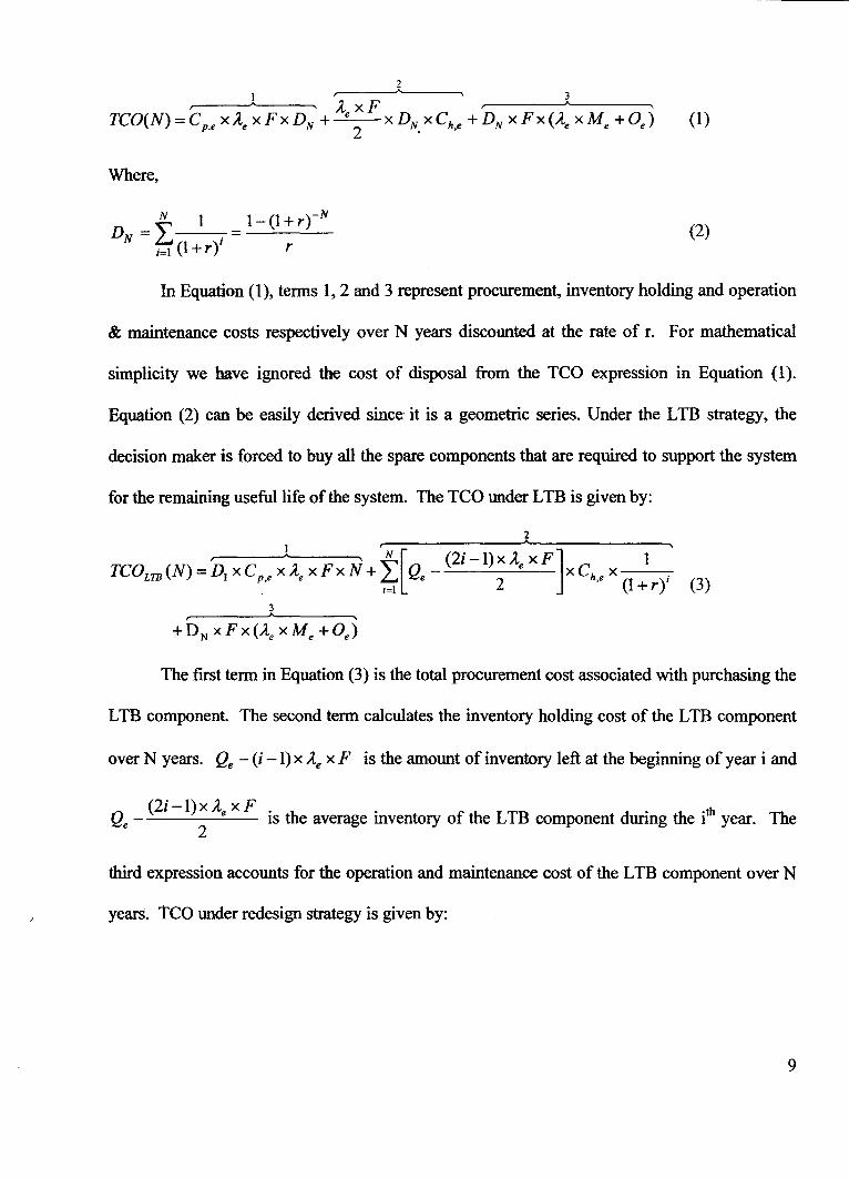
In Equation (1), tenns 1,2 and 3 represent procurement, inventory holding and operation

& maintenance costs respectively over N years discounted at the rate of r. For mathematical

simplicity we have ignored the cost of disposal from the Teo expression in Equation (1).

Equation (2) can be easily derived since it is a geometric series. Under the LTB strategy, the

decision maker is forced to buy all the spare components that are required to support the system

for the remaining useful life of the system. The TeO under LTB is given by:

2 l' A ,

,r--__ A , N [ (2i-l)XA XF] 1 TCOLTB(N)=DlxCp,eXAexFxN+ L Qe- e xCh,e x ;

. ;=1 2 (l+r) (3) 3 A , ,

+DN XFX(Ae xMe +Oe)

The first tenn in Equation (3) is the total procurement cost associated with purchasing the

L TB component. The second tenn calculates the inventory holding cost of the L TB component

over N years. Qe - (i -1) x Ae x F is the amount of inventory left at the beginning of year i and

Q (2i -1) x Ae x F . th . f th ··th

e - IS e average mventory 0 e LTB component dunng the 1 year. The 2

third expression accounts for the operation and maintenance cost of the L TB component over N

years. teo under redesign strategy is given by:

9

(4)

I ,

+DN XFX(Ad XMd +Od)

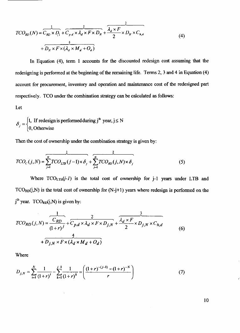
In Equation (4), term 1 accounts for the discounted redesign cost assuming that the

redesigning is performed at the beginning of the remaining life. Terms 2,3 and 4 in Equation (4)

account for procurement, inventory and operation and maintenance cost of the redesigned part

respectively. TCO under the combination strategy can be calculated as follows:

Let

8 = {I, If redesign is performed during jth year, j ~ N

J 0, Otherwise

Then the cost of ownership under the combination strategy is given by:

N N

TCOcCj,N) = ITCOLTB U-I)x8} + ITCORD U,N)x8} (5) }=I }=I

Where TCOLTB(j-l) is the total cost of ownership for j-l years under L TB and

TCORDG,N) is the total cost of ownership for (N-j+ I) years where redesign is performed on the

jth year. TCOwG,N) is given by:

Where

D·N=I ·-I = N 1 j-l 1 (I + rrU-1) - (l + r)-N J

J, ;=1 (l + r)' k=1 (1 + r)k r (7)

10

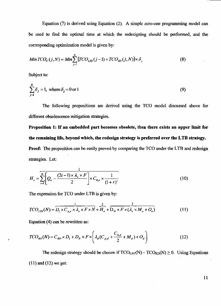
Equation (7) is derived using Equation (2). A simple zero-one programming model can

be used to fmd the optimal time at which the redesigning should be performed, and the

corresponding optimization model is given by:

N

Min TCOdj,N) = Min :L(TCOLm(j -1) + TCORD(j,N»)x b j j~1

Subject to:

N

:Lbj = 1, whereoj =Oorl j=1

(8)

(9)

The following propositions are derived using the TCO model discussed above for

different obsolescence mitigation strategies.

Proposition 1: If an embedded part becomes obsolete, then there exists an upper limit for

the remaining life, beyond which, the redesign strategy is preferred over the LTD strategy.

Proof: The proposition can be easily proved by comparing the TCO under the LTB and redesign

strategies. Let:

H = ~[Q _ (2i-l) xAe XF]xC x l'

e L.J e 2 h,e (1 )' ~ +r

(10)

The expression for TCO under L TB is given by:

(11)

Equation (4) can be rewritten as:

(12)

The redesign strategy should be chosen ifTCQBT(N)- TCOw(N) ~ O. Using Equations

(11) and (12) we get:

11

Or

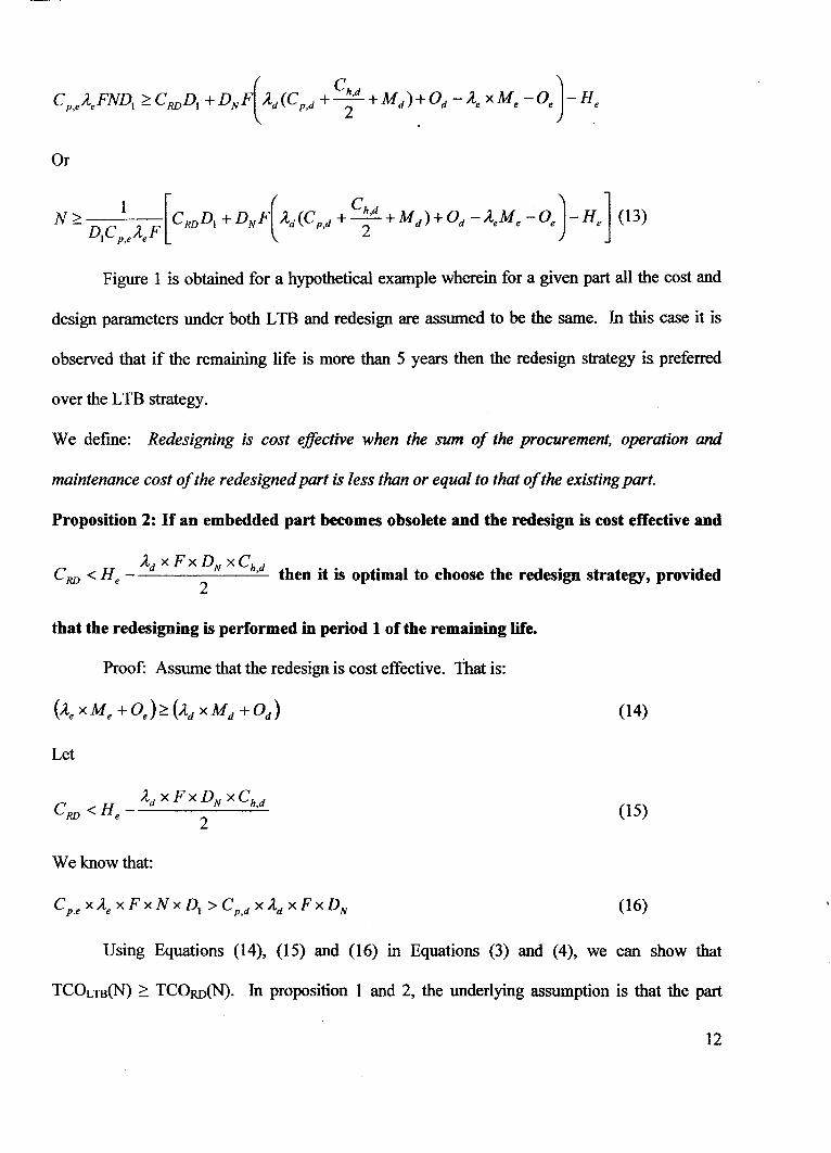
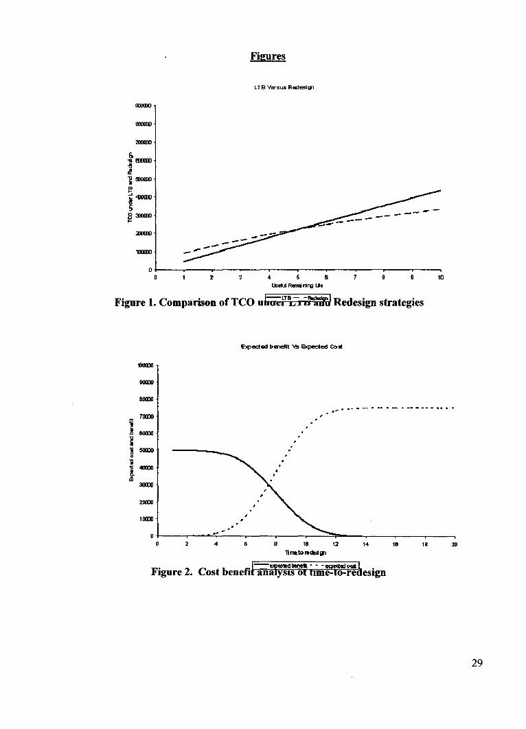
Figure 1 is obtained for a hypothetical example wherein for a given part all the cost and

design parameters under both L TB and redesign are assumed to be the same. Tn L;is case it is

observed that if the remaining life is more than 5 years then the redesign strategy is preferred

over the LTB strategy.

We defme: Redesigning is cost effective when the sum of the procurement, operation and

maintenance cost of the redesigned part is less than or equal to that of the existing part.

Proposition 2: If an embedded part becomes obsolete and the redesign is cost effective and

Ad xFxDN XChd C RD < He - > then it is optimal to choose the redesign strategy, provided 2

that the redesigning is performed in period 1 of the remaining life.

Proof: Assume that the redesign is cost effective. That is:

(14)

Let

(15)

We know that:

(16)

Using Equations (14), (15) and (16) in Equations (3) and (4), we can show that

TCOLTB(N) 2: TCOw(N). In proposition 1 and 2, the underlying assumption is that the part

12

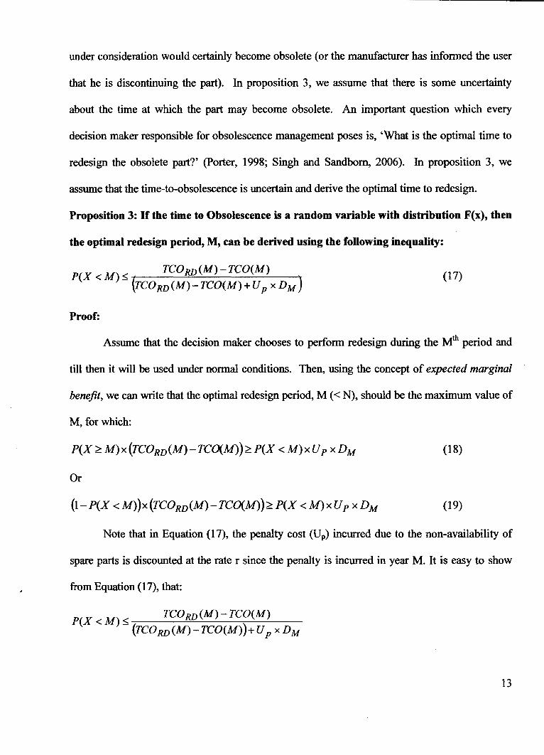
under consideration would certainly become obsolete (or the manufacturer has informed the user

that he is discontinuing the part). In proposition 3, we assume that there is some uncertainty

about the time at which the part may become obsolete. An important question which every

decision maker responsible for obsolescence management poses is, 'What is the optimal time to

redesign the obsolete part?' (porter, 1998; Singh and Sandborn, 2006). In proposition 3, we

assume that the time-to-obsolescence is uncertain and derive the optimal time to redesign.

Proposition 3: If the time to Obsolescence is a random variable with distribution F(x), then

the optimal redesign period, M, can be derived using the following inequality:

P X <M < TCORD(M)-TCO(M) ( )- frCORD(M)-TCO(M)+U p xDM )

(17)

Proof:

Assume that the decision maker chooses to perform redesign during the Mth period and

till then it will be used under normal conditions. Then, using the concept of expected marginal

benefit, we can write that the optimal redesign period, M « N), should be the maximum value of

M, for which:

P(X ~ M) x (TCORD(M) - TCfX..M)) ~ P(X < M) x Up x DM (18)

Or

(1-P(X <M))x(TCORD(M)-TCfX..M))~P(X <M)xUp xDM (19)

Note that in Equation (17), the penalty cost (Up) incurred due to the non-availability of

spare parts is discounted at the rate r since the penalty is incurred in year M. It is easy to show

from Equation (17), that:

P(X < M) ~ TCO RD (M) - TCO(M) (TCORD(M)-TCO(M»)+U p x DM

13

If the time to obsolescence follows an exponential distribution, with mean obsolescence time (Jl),

then equation (17) can be written as:

Rearranging equation (20), we get:

M ~,uxln(-l-) l-R

Where,

R _ TCORD(M)-TCO(M)

- (TCORD(M) - TCO(M)) + Up x DM

(20)

(21)

Figure 2 depicts the graphs of expected benefits and expected cost ~urves for a part for

which the time-to-obsolescence is assumed to follow a normal distribution with mean 8 years

and standard deviation 2 years. In this example, the optimal time to redesign is 7 years. When

the remaining life of the system is very large and the technology obsolescence rate is high, it is

likely that the redesigned part may become obsolete before the system is decommissioned. Here

normal distribution is used for time-to-obsolescence for illustrative purpose only. In the next

section, we use the Markov decision processes called the Bandit processes to model and find the

optimal sequence of decisions.

4.0 Bandit Process Approach for Optimal Selection of Obsolescence Mitigation Strategies

Assume that at the beginning of each period the decision maker has to choose one of the

many strategies available to her. Let Sij be the strategy j used for period i and Rij(Sij) is the

expected reward for choosing strategy j for period i. Let II be the sequence of decisions made

over N periods. That is:

14

(22)

The corresponding expected total reward R(n) is given by:

N M

R(n) = 'L'Lpipij(Sij)Rij(Sij) (23) i=1 j=1

Where Pij(Sij) is the probability of obtaining the reward Rij(Sij) when strategy Sij IS

chosen. A sequence n· is called p-optimaI (Mine and Osaki, 1970) if there exists a sequence of

strategies n· such thatR(nt

) ~ R(TI) V n, where (0 ~ J3 < 1). The problem stated in (22) and

(23) is a classical Multi-arm Bandit Problem (MAB) and the resulting process is called the

Bandit process in which a decision maker has to take a sequence of decisions that maximizes her

total expected discounted reward. The rewards are discounted since they are earned at different

time periods. In this case we have assumed finite time horizon which is determined by the

designed life of the systems, after that the system is condemned or decommissioned. It is

possible that the designed life of the system may be extended, but in this paper we restrict our

analysis to systems without life extensions beyond their initial design period.

A common example used in explaining a MAB is the sequential selection of projects to

optimize the total reward over T ( t = 1, 2, .. , T) periods. Assume that there are N parallel

projects indexed by k = 1,2, ... , N. The project k can be in nt(k) states, where nt(k) is finite. At

any instant of time t, only one project is chosen for implementation. Ifproject k in state nt(k) is

chosen for period 1, then one receives an expected reward R(fit(k». The rewards are additive and

d.iscounted by a factor p, where 0 < p < 1. The state nt(k) changes to nt+I(k), the state evolution

is a Markov process in which change of state depends on k, but not on t. In the classical MAB,

the states of projects that are not chosen remain same. The problem is to choose the projects

15

sequentially to maximise the total discounted reward. Thus, MAB is basically an independent

Markov decision process with aforementioned additional conditions.

Thompson (1933) introduced the two-arm bandit problem in the context of clinical trials,

and since then they were used extensively by others in clinical drug trials, petroleum exploration

and consumer product or service settings (e.g., Gittins (1989), Meyer and Shi (1995), Erdem and

Keane (1996), Banks et al (1997), Anderson (2001». Breakthrough research on Bandit problems

were carried out by Gittins and Jones (1974), Whittle (1981, 1988), Berry and Fristedt (1985)

and Glazebrook (1987, 1990). Gittins and Jones (1974) proved that a k-armed Bandit problem

can be solved by solving k-one armed bandit problems. This theorem asserts that in any

indepelldent-armed Bandit problem with geometric discounting over an inftnite horizon, it is

possible to associate with each arm an index (dynamic allocation index), known as the Gittins

Index, with the property that a strategy in the Bandit problem is an optimal strategy if and only if

it involves playing an arm with the highest value of the Gittins Index at that point (such a

strategy is called the Gittins Index strategy). Whittle (1981) introduced the concept of arm-

acquiring baildits, in which new arms may be added to the problem at a later stage and proved

that Gittins index policy of classical MAB is optimal to arm-acquiring bandits as well. The

Gittins index (dynamic allocation index, Gittins (1979» for the jth arm with a discount rate of (3

is calculated as follows:

N N

GJ = SliP "LPiE(Rij)/ E"LPi N~1 i=1 i=1

for j = 1, ... ,N (24)

The feature that gives this result especial potency is that the Gittins Index on an ann

depends solely on the characteristics of that arm and on the rate of discounting, and not on any

other feature of the problem under study (Sundaram, 2003).

16

Whittle (1988) generalized the classical MAB by allowing state evaluation of passive

arms. The new model called "restless bandit" problems allowed rewards for arms under passive

state and the decision maker can choose m out of n arms (m < n). Restless bandit (RB) problems

are intractable and are proved to be PSP ACE-hard (papadimitriou and Tsitsiklis, 1999). Whittle

(1988) proposed an index policy for RB problems which reduces to Gittins index for the classical

MAB. However, Whittle's index policy is applicable to only certain class of RB problems that

satisfy a certain indexability property, which may be hard to check. Nino-Mora (2001) derived

sufficient conditions for indexability of Whittle's indices based on partial conservation laws.

Glazebrook (1987, 1990, and 1996) made several important contributions to the theory of

MAB and RB problems and presented approaches to policy evaluation and sensitivity analysis in

stochastic scheduling via index based sub-optimality bounds and procedures for the evaluation of

Gittins Index strategies for resource allocation in a stochastic environment. Recently, Glazebrook

et al (2005, 2006) used RB model to analyse machine maintenance problems, where bandits

represent machines that evolve under the influence of maintenance actions. Glazebrook et al

(2006) use Whittle's index policy to arrive at optimal decisions for machine maintenance

problem.

The selection of optimal obsolescence strategies in its general form is an arm-acquiring

restless bandit problem. New technologies would emerge from time to time and the decision

maker has to decide on the optimal strategy based on all currently available technological

choices. Also, the state evolution of arms depends on the time, that is, the rate at which a

technology becomes obsolete would depend on the time (current age of the technology), and thqs

the problem is also a restless bandit problem. State evolution occur independent of whether an

arm (in this case the strategy) is chosen or not. However, at any stage, the decision maker

17

chooses only one ann, and there is no passive reward for the anns which are not chosen.

Dayanik et al (2007) have proved that when the passive rewards are equal to zero, the Whittle's

index converges to Gitlin's index. In fact, for the optimal selection of obsolescence strategies,

since only one strategy can be chosen at any period and passive anns carry no reward; there is no

difference between Whittle's and Gitlin's indices.

4.1 Two Armed Bandit Model For Selection Of Obsolescence Strategy

Every year, during the useful life of a system, the decision maker faces the issue of

having to decide on the strategy she is going to use to deal with the obsolescence of parts. While

the decision maker is infonned about parts that are likely to become obsolete in the near future,

she may ignore the warning and store only those parts required for that particular period to

support the system, or go for the redesign strategy (if redesign strategy turns out to be an

optimum strategy, the decision maker can always choose LTB till that period). That is, there is a

state change in the fonn of availability of parts in the next period, irrespective of the fact whether

an ann is chosen or not. A two anned restless bandit approach can be used to model this

problem, where each ann represents a unique strategy as defmed below. At any period only one

arm is chosen and there is no passive reward.

Ann 1: The decision maker chooses to procure parts required for the current period

(period i) only.

Ann 2: The decision maker chooses to redesign the part during period i.

Now we calculate the Gittins Indices for arm 1 and ¥Ill 2 and choose the ann which has

the highest Gittins Index (please note ~t in this case both Whittle's and Gittin's indices are

same). Since we are dealing with a two anned restless bandit problem, we continue the

estimation of Gittins Indices until ann 2 is chosen, and this point becomes the stopping rule in

18

our case. It is obvious that the decision maker would like to minimize the total cost of ownership

of the system. At the same time however, if the decision maker is unable to maintain the

availability of the system due to the chosen strategy, she is likely to incur a heavy penalty. The

expected reward E(Rij) corresponding to arm j during period i is defined as the difference

between penalty cost and the total cost of ownership under the corresponding obsolescence

strategy.

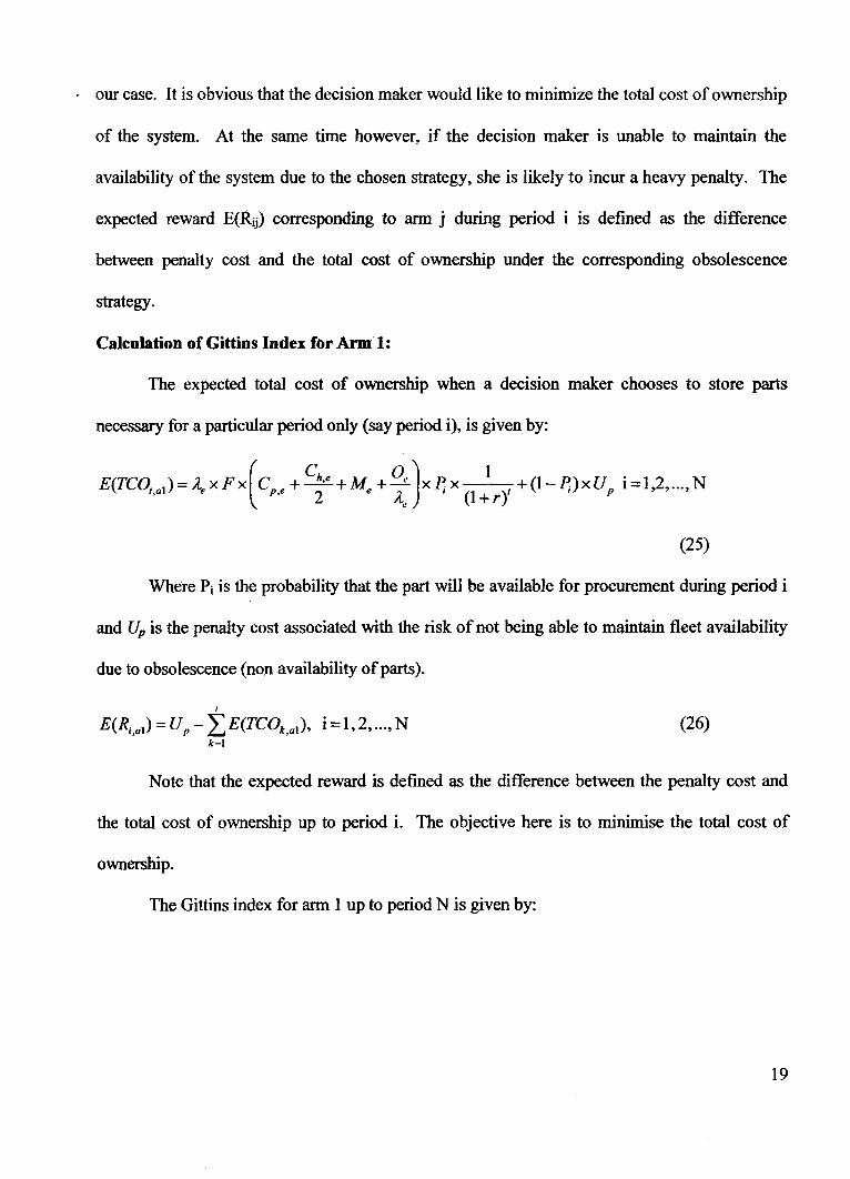
Calculation of Gittins Index for Arm' 1:

The expected total cost of ownership when a decision maker chooses to store parts

necessary for a particular period only (say period i), is given by:

(25)

Where Pi is the probability that the part will be available for procurement during period i

and Up is the penalty cost associated with the risk of not being able to maintain fleet availability

due to obsolescence (non availability of parts).

i

E(R;,al)=Up - ,LE(TCOk,al)' i=I,2, ... ,N (26) k=1

Note that the expected reward is defined as the difference between the penalty cost and

the total cost of ownership up to period i. The objective here is to minimise the total cost of

ownership.

The Gittins index for arm 1 up to period N is given by:

19

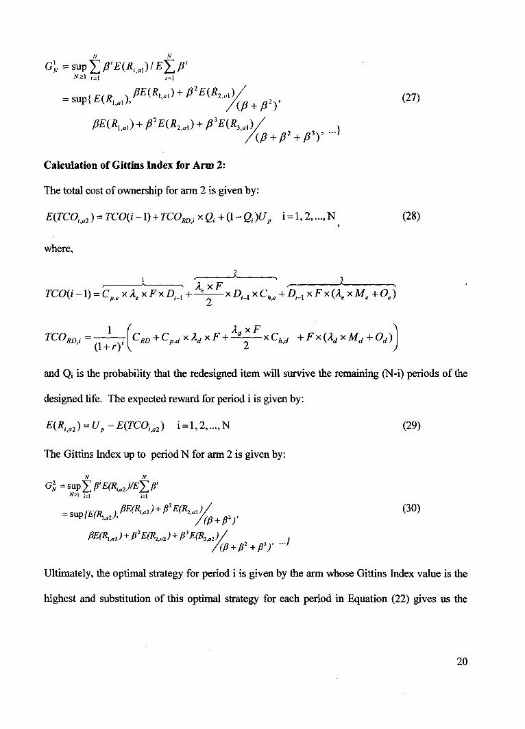
N N

G~ = sup IpiE(Ri,al)/ EIpi N2:1 i=1 i=l

(27)

Calculation of Gittins Index for Arm 2:

The total cost of ownership for arm 2 is given by:

E(TCOi,a2) = TCO(i -1) + TCORD,i x Qi + (1- Qi)U p i = 1, 2, ... , N (28)

where,

and Qi is the probability that the redesigned item will survive the remaining (N-i) periods of the

designed life. The expected reward for period i is given by:

E(R i ,a2) = Up - E(TCOi ,a2) i = 1, 2, ... , N (29)

The Gittins Index up to period N for arm 2 is given by:

(30)

Ultimately, the optimal strategy for period i is given by the arm whose Gittins Index value is the

highest and substitution of this optimal strategy for each period in Equation (22) gives us the

20

optimum sequence of decisions U* and the corresponding optimum expected reward R(U*),

over N periods can be obtained from Equation (23).

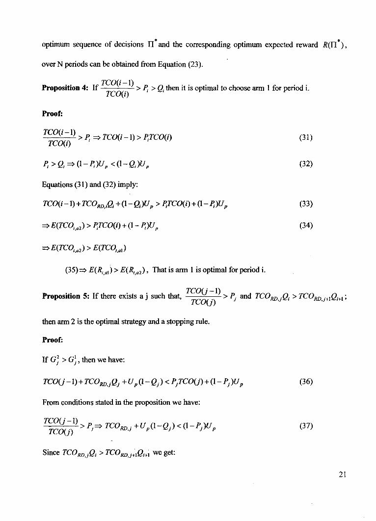
Proposition 4: If TCO(i -1) > P; > Qi then it is optimal to choose arm 1 for period i. TCO(i)

Proof:

TCO(i -1) > P ~ TCO(i -1) > PTCO(i) TCO(i) I I

(31)

(32)

Equations (31) and (32) imply:

TCO(i -1) + TCORD,;Qj + (1- Q;)U p > P;TC-()(i) + (1- P;)U p (33)

~ E(TCOi,a2) > P;TCO(i) + (1- P;)U p (34)

(35)~ E(Ri,al) > E(Ri,a2)' That is arm 1 is optimal for period i.

Proposition 5: If there exists a j such that, TCO(j -1) > Pl· and TCORD ,.Q; > TCORD ,·+IQ;+1 ; TCO(j) , ,

then arm 2 is the optimal strategy and a stopping rule.

Proof:

If G~ > G~ , then we have:

(36)

From conditions stated in the proposition we have:

(37)

21

(38)

Thus, if there exists a 'j' such that G J > G ~ and, TCO(j -1) > P and TCO(j) J

TCORD,jQ; > TCORD,j+lQi+l then ann 2 is the optimal strategy and a stopping rule.

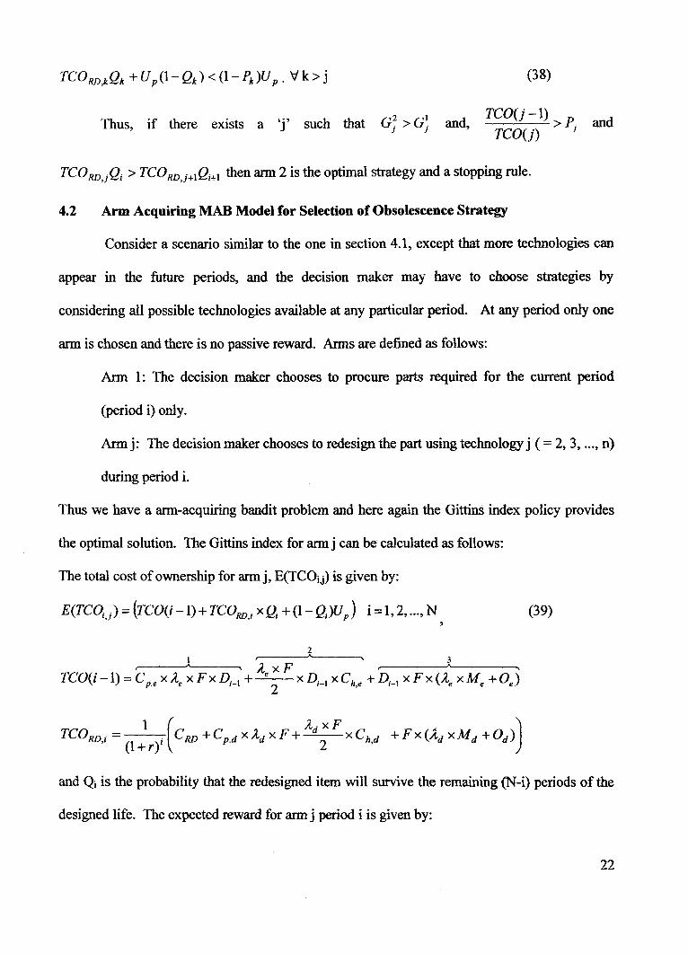
4.2 Arm Acquiring MAB Model for Selection of Obsolescence Strategy

Consider a scenario similar to the one in section 4.1, except that more technologie,s can

appear in the future periods, and the decision maker may have to choose strategies by

considering all possible technologies available at any particular period. At any period only one

ann is chosen and there is no passive reward. Arms are defmed as follows:

Arm 1: The decision maker chooses to procure parts required for the current period

(period i) only.

Arm j: The decision maker chooses to redesign the part using technology j ( = 2, 3, ... , n)

during period i.

Thus we have a ann-acquiring bandit problem and here again the Gittins index policy provides

the optimal solution. The Gittins index for ann j can be calculated as follows:

The total cost of ownership for armj, E(TCOjj) is given by:

E(TCq,j) = (TCO(i -1)+ TCOm,i XQi +(1- QJUp ) i=I,2, ... , N (39)

and Qi is the probability that the redesigned item will survive the remaining (N-i) periods of the

designed life. The expected reward for ann j period i is given by:

22

E(Ri ,) = 8;,Aup - E(TCq,j») i= 1, 2, ... , N;j = 2, 3, ... , n (40)

where,

8. . = {1, if arm j is available during period i .,J 0 otherwise ,

5.0 Calculation of Gittins Index - Illustrative Example

In this section, we use a hypothetical example to illustrate the Bandit process models

discussed in section 4. The values of the parameters are shown in Table 1. Table 1 contains

three sets of values, the first set of values correspond to the existing part which has become

obsolete (arm 1), the second set of values correspond to the redesign option using technology 1

(arm 2) and third set of values correspond to the redesign option using technology 2 which will

be available at the beginning of year 3 (arm 3). Using the data defined in Table 1 we have

calculated Gittins indices for the following two scenarios.

Scenario 1:

The decision maker chooses the optimal strategy for management of obsolescence by

considering the technological options available at the beginning of the decision making period.

That is, a two-armed bandit model is used to calculate the Gittins Index values. The Gittins index

values for arms 1 and 2 are shown in Table 2. From the values of the Gittins Index, the optimal

strategy is arm 1 for the fIrst six periods and arm 2 from period 7 onwards which is a stopping

rule. The optimal strategy for the hypothetical problem is to redesign the part during period 7

and have normal operation for the fust six periods. From the data in Table 2, one may notice

that there is a 30% chance that the part may not be available in the market in period 6.

23

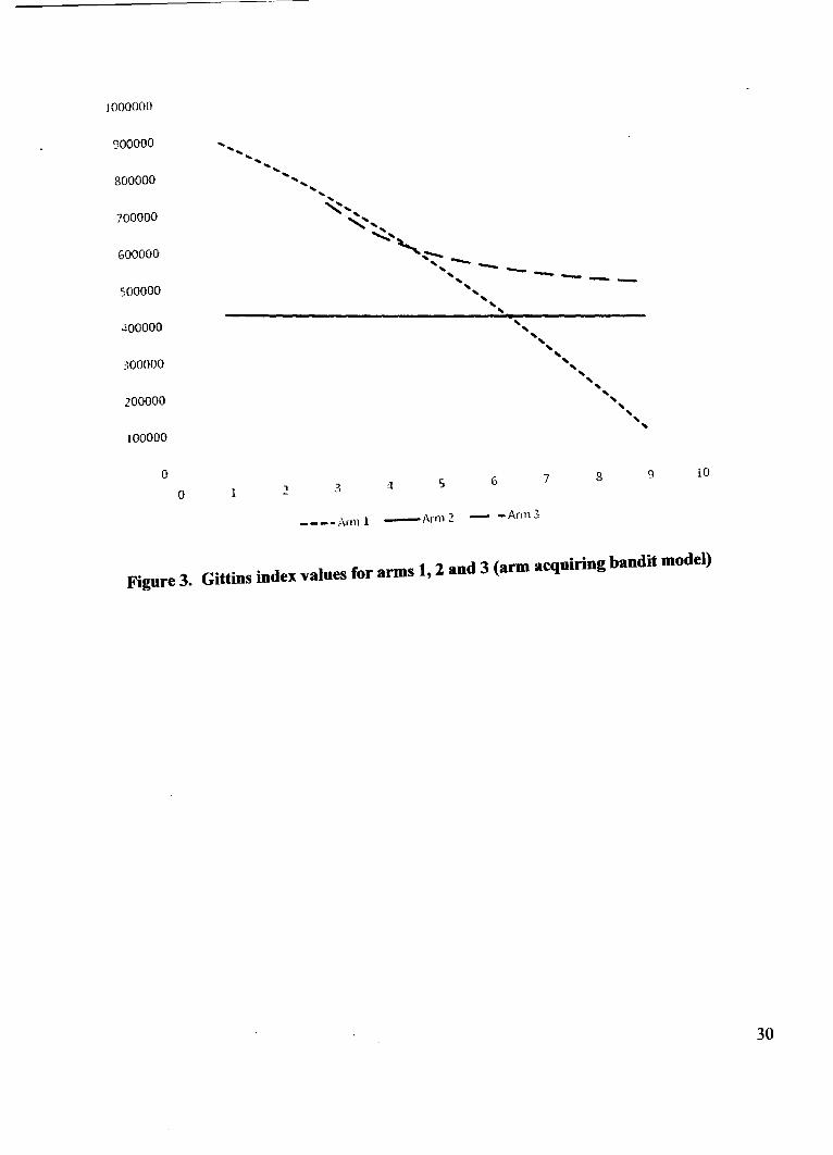
Scenario 2:

In scenario 2, we assume that the part may be redesigned using an alternative technology

which will be available from period 3 onwards. This scenario is modelled using arm-acquiring

bandit model. This is a three-armed bandit problem in which the third arm is available from

period 3 onwards. The optimal solution to this problem is to use arm 1 for first four periods and

arm 3 in period 5. Figure 3 shows Gittins index values for 3 arms. In both scenarios we have

used decreasing probabilities for survival of the redesigned part since the technology used to

redesign may also become obsolete before the designed life of the system.

6. Conclusions and Future Research

The life span of a capital asset is a critical period because the asset manager has to make

several important decisions to ensure that availability of the system is maintained at the least cost

of ownership. During the designed life of the system, some embedded parts may either become

obsolete or become technologically inferior. In this paper, we have developed a few

mathematical models that would assist a decision maker in choosing the best obsolescence

mitigation strategy from a set of available strategies. In the first set of mathematical models, we

have assumed that the decision maker either receives information about the part obsolescence or

has knowledge about the prior distribution of time to obsolescence of a part embedded within the

system or LRU. Using techniques like zero-one programming and expected marginal benefit,

the model identifies the optimal time to redesign in each case.

The aforementioned myopic models may not be suitable when the remaining life of the

system is large or if the rate of technological obsolescence is very high. In such situations, the

decision maker has to use a sequence of decisions that is optimal. During each period, the

decision maker gains some new information about the parts and is in a better position to judge

24

between various options. We have modelled this problem using the restless multi-armed Bandit

approach. As an illustrative example, a restless two-armed Bandit framework is used to show

how the optimal strategy can be chosen in case of two strategic choices. The main advantage of

the Bandit process approach is that the model allows the decision maker to update the model

parameters when she moves from one period to the next. We have also illustrated how to

calculate the Gittins Indices in the case of two-armed Bandit problems, which can be extended to

cases of multi-armed bandit problems also. Another important aspect of obsolescence

management problem is that more technologies may become available that can be used to

redesign the obsolete part and the decision maker has to include all available technology to

choose the best strategy. This scenario is modelled using arm acquiring bandit models.

In this paper, we have assumed that the arms are independent; however, this need not be

true always. Consequently, there is scope for future research to, develop mathematical models

for choosing optimal, obsolescence strategies under dependent arms. In the current paper, we

have assumed that the system's life is not extended beyond the design life of the system,

however, for many systems, life extensions are common practice and future research should

consider these cases.

Acknowledgements

We would like to thank both anonymous referees for their very constructive comments which helped us to improve the paper enormously.

References

1. Anderson, C. M. (2001) Behavioral Models of Strategies in Multi-Armed Bandit Problem's. Ph.D. Dissertation, California Institute of Technology.

2. Asiedu, Y., and Gu, P., "Product Life Gyc1e Cost Analysis: State of the Art Review", International Journal of Production Research, 36(4),883-908.

3. Banetjee, P K. and Kabadi, S N. (1994) On optimal replacement policies - random horizon, Operations Research, 42(3),469-475.

25

4. Banks, J, Olson, M and Porter, D. (1997). An Experimental Analysis of the Bandit Problem. Economic Theory, 10, 55-77.

5. Berry D. A., and Fristedt, B. (1985), Bandit problems: sequential allocation of experiments, Chapman and Hall, London.

6. Bulow, J. (1986) An Economic Theory of Planned Obsolescence, Quarterly Journal of Economics, Vol 101, 729-749.

7. Capon, N., Farley, J U., Lehmann D R. and Hulbert, J M. (1992) Profiles of product innovators among large US manufacturers, Management Science, 38(2), 157-169.

8. Dayanik, S., Powell, W., and Yamazaki, K., (2007), Index policies for discounted bandit problems with availability constraints, to appear in Advances in Applied Probability.

9. Dinesh Kumar, U., Jose E. Ramirez-Marquez, D Nowicki and D Verma, (2007), 'Reliability and Maintainability Allocation to Minimize the Total Cost of Ownership in a Series-Parallel System', Journal of Risk and Reliability, 221(2), 133-140.

10. Erdem, T and Keane, M. P. (1996) Decision-Making Under Uncertainty: Capturing Dynamic Brand Choice Processes in Turbulent Consumer Goods Markets, Marketing Science, 15, 1-20.

11. Feltus, P., (2007), "The US Centennial Flight Commission - The B-52 Bomber", Internet article: .______- _ - (last sited on 3rd September 2007).

12. GatignQn, H., Tushman, M L., Smith, W. and Anderson, P. (2002) A structural approach to assessing innovation: construct development of innovation locus, type and characteristics, Management Science, 48(9), 1103-1122.

13. Gittins J. C. and Jones. D. M., (1974), A Dynamic Allocation Index for the Sequential Design of Experiments. Progress in Statistics, J. Gani et al. eds., 241-266.

14. Gittins. J. C. (1989) Multi-Armed Bandit Allocation Indices. John Wiley & Sons. 15. Glazebrook, K.D. (1987) Sensitivity analysis for Stochastic Scheduling Problems,

Mathematics of Operations Research., 12, 205-225. 16. Glazebrook, K.D. (1990) Procedures for the evaluation of Strategies for Resource

Allocation in a Stochastic Environment, Journal of Applied Probability, 27, 215-220. 17. Glazebrook, K.D. (1996) Reflections on a New Approach to Gittins Indexation, Journal

of the Operational Research Society, 47(10), 1301-1309. 18. Glazebrook, K D., Mitchell, H M., and Ansell, P S., (2005), Index policies for the

maintenance of a collection of machines by a set of repairmen, European Journal of Operational Research, Vol. 165,267-284.

19. Glazebrook, K D., Ruiz-Hernandez, D and Kirkbride, C., (2006) Some indexable families of restless bandit problems, Advances in Applied Probability, Vol. 38, 643-672.

20. Goldstein, T., Ladany, S. and Mehrez, A. (1998) A disco~ted machine replacement model with expected future technological breakthrough, Naval Research LQgistics, 35, 209-220.

21. Grout, P A., and Park, I (2005) Competitive planned obsolescence, RAND Journal of Economics, Vol. 36, No.3, 596-6l2.

22. Hamilton, P., and Chin, G., (2001), "Military Electronics and Obsolescence Part I: The Evolution of a Crisis," COTS Journal, March 2001, 77-81.

23. Hartman, J C. (2001) An economic replacement model with probabilistic asset utilization, IIE Transactions, 33, 717-727.

26

24. Hitt, E. F., and Schmidt, J., (1998), 'Technology Obsolescence Impact on Future Costs,' Proceedings of the I1h Digital Avionics Systems Conference, A33-1 :A33-7.

25. Hoorickx, P F. (2008) Sustaining engineering challenges in long-life medical electronics, Proceedings of the SMIA Medical Electronics Symposium, Anaheim, CA, January 29-31, 2008.

26. Hunt, E K., and Haug, S., (2001), 'Challenges of Component Obsolescence, Proceedings of the Royal Aeronautical Society Conference in London, 2001.

27. Johnson, W. J. (2002) Defence Logistics Agency Component Obsolescence Management, Proceedings of Sixth Joint FAA/DoD/NASA Ageing Aircraft Conference, September, 16-19.

28. Lai, K K., Leung, K N F., Tao, B. and Wang, S Y. (2001) A sequential method for preventive maintenance and replacement of a repairable single unit system, Journal of Operational Research Society, 52(11), 1276-1283.

29. Lee, I H and Lee, 1. (1998) The Theory of Economic Obsolescence, The Journal of Industrial Economics, 46(3),383-401.

30. Meyer, A., Pretorius, L., and Pretorius, J H C. (2004) A Model using an Obsolescence Mitigation Timeline for Managing Component Obsolescence of Complex or Long Life Systems, Proceedings of the International Engineering Management Conference, 1310-1313.

31. Meyer, R. J. and Shi, Y. (1995) Sequential Choice under Ambiguity: Intuitive Solutions to the Armed-Bandit Problem, Management Science, 41, 817-834.

32. Mine, H and Osaki, S. (1970) Markovian Decision Processes, American Elsevier Publishing Company, New York.

33. Nair, S K. and Hopp W J. (1992) A model for equipment replacement due to technological ~bsolescence, European Journal of Operational Research, 63,207-221.

34. Nino-Mora, J (2001), Restless bandits, partial conservations laws and indexability, Advances in Applied Probability, Vol. 33, 76-98.

35. Oakford, R., Lohmann, J. and Salazar, A. (1984) A dynamic replacement economic decision model, IlE Transactions, 16, 65-72.

36. Papadimitriou, C H., and Tsitsildis, J N., (1999), The complexity of optimal queueing network control, Mathematics of Operations Research, Vol. 24, 293-305.

37. Porter, G. Z., (1998), "An Economic Method for Evaluating Electronic Component Obsolescence Solutions", Boeing White paper from

_____________ ._.- ___ c____ __ _ _ _ _ _ (last sited on 3rd September 2007). 38. Regnier, E., Sharp, G. and Tovey, C. (2004) Replacement under ongoing technological

progress, IIE Transactions, 36, 497-508. 39. Szoch, R L., Brown, EM., and Wilkinson, CD., (1995) Strategic AlHance to Address

Safety System Obsolescence and Maintainability, Proceedings of IEEE, 1073-1076. 40. Short, P. (2006) Don't Fret over IC Obsolescence, Prepare for IT, Electronic Design, 22. 41. Singh, P., and Sandborn, P. (2005) Forecasting Technology Insertion Concurrent with

Design Refresh Planning for COTS Based Electronic Systems, Proceedings of the Annual Reliability and Maintainability Symposium, 349-354.

42. Singh, P., and Sandborn, P. (2006) Obsolescence Driven Design Refresh Planning for Sustainment Dominated Systems, The Engineering Economics, 51, 115-139.

27

43. Solomon, R, Sandborn, P. A., and Pecht, M. G. (2000) Electronic Part Life Cycle Concepts and Obsolescence Forecasting, IEEE Transactions on Component and Packaging Technologies, 23(4),707 -717.

44. Sundaram, RK. (2003). Generalized Bandit Problems

_' last sited on 3ed September 2007. 45. Tepp, B. (1999) Managing the Risk of Parts Obsolescence, COTS Journal,

September/October 1999,69. 46. Thompson, W. R (1933) On the likelihood that one unknown probability exceeds

another in view of the evidence of two samples. Biometrika, 25, 285-294. 47. Tomczykowski, W J. (2003) A Study on Component Obsolescence Mitigation Strategies

and their Impact on R and M, Proceedings of the Annual Reliability and Maintainability Symposium, 332 - 338.

48. Whittle, P (1981), Arm acquiring bandits, The Annals of Probability, Vol. 9, No.2, 284-292.

49. Whittle, P (1988), Restless bandits: activity allocation in a changing world, Journal of Applied Probability; Vol. 25A, 287-298.

28

Figures

l T B Versus Redesig>

O~---.----~----~----'-----~----~---.~--~-----r----~ o 2 4 5 8 7 8 g 10

UseIuI Ran.i ri~ lie

Figure 1. Comparison of TCO u~'b I D~ Redesign strategies

iii j ~ ~ 0

i 'S ! d!

»oalO

lIOWO

oomo

TIlIOO

IW)OOj)

$OWl)

4OOlO

3OIQ)

zomo

IIIIDI

0 0 2 4 6

.. - - -- ..... - . -- - .. - _ ... ~~

8 10 12 14 18 18 20 11 me to l'lditii IJl

Figure 2. Cost benefi! an"~ nm=~hesign

29

looooon

'Jooooo ...... 800000

..............

700000

600000

500000

';00000

300000

200000

100000

0

0 1

..... ... ... " ..... -.....:- .... ....:::.. ... ,,~

...... -... -.... -.... --... --... .... ... ... ... ... ... ... ...

3 4 5 6 7

____ Arm1 _.Arm 2 - -Ann3

... ... ... ... ... ... ... ...

8

... ... ... ...

10

Figure 3. Gittins index values for arms 1,2 and 3 (arm acquiring bandit model)

30