Embed Size (px)
Citation preview
OPTIMIZATION OFWELL PLACEMENT IN COMPLEX CARBONATE RESERVOIRS USING
ARTIFICIAL INTELLIGENCE
A THESIS SUBMITTED TO THE GRADUATE SCHOOL OF NATURAL AND APPLIED SCIENCES
OF MIDDLE EAST TECHNICAL UNIVERSITY
BY
İRTEK URAZ
IN PARTIAL FULFILLMENT OF THE REQUIREMENTS FOR
THE DEGREE OF MASTER OF SCIENCE IN PETROLEUM AND NATURAL GAS ENGINEERING
DECEMBER 2004

ii
Approval of the Graduate School of Natural and Applied Sciences
Prof. Dr. Canan Özgen Director
I certify that this thesis satisfies all the requirements as a thesis for the degree of Master of Science.
Prof. Dr. Birol Demiral Head of Department
This is to certify that we have read this thesis and that in our opinion it is fully adequate, in scope and quality, as a thesis for the degree of Master of Science.
Prof. Dr. Mustafa V. Kök Assoc.Prof.Dr. Serhat Akın CoSupervisor Supervisor
Examining Committee Members
Prof. Dr. Fevzi Gümrah (METU,PETE)
Assoc. Prof. Dr. Serhat Akın (METU,PETE)
Prof. Dr. Mustafa V. Kök (METU,PETE)
Prof. Dr. Mahmut Parlaktuna (METU,PETE)
Assoc. Prof. Dr. İ. Hakkı Toroslu (METU,CENG)

iii
I hereby declare that all information in this document has been obtained and presented in accordance with academic rules and ethical conduct. I also declare that, as required by these rules and conduct, I have fully cited and referenced all material and results that are not original to this work.
Name, Last Name: İrtek Uraz
Signature:
iv
ABSTRACT
OPTIMIZATION OF WELL PLACEMENT IN COMPLEX CARBONATE RESERVOIRS USING ARTIFICIAL
INTELLIGENCE
Uraz, İrtek
M.S., Department of Petroleum and Natural Gas Engineering
Supervisor : Assoc. Prof. Dr. Serhat Akın
Co‑Supervisor : Prof. Dr. Mustafa Versan Kök
December 2004
This thesis proposes a framework for determining the optimum location of
an injection well by using an inference method, Artificial Neural Networks
and a search algorithm to create a search space and locate the global
maxima. Theoretical foundation of the proposed framework is followed by
description of the field for case study. A complex carbonate reservoir,
having a recorded geothermal production history is used to evaluate the
proposed framework ( Kızıldere Geothermal field, Turkey). In the proposed
framework, neural networks are used as a tool to replicate the behavior of
commercial simulators, by capturing the response of the field given a
limited number of parameters (Temperature, pressure, injection location and
injection flow rate) as variables. A study on different network designs is
followed by introduction of a search algorithm to generate decision surfaces.
v
Results indicate that a combination of neural networks and an optimization
algorithm (explicit search with variable stepping) to capture local maxima
can be used to locate a region or a location for optimum well placement.
Results also indicate shortcomings and possible pitfalls associated with the
approach. With the provided flexibility of the proposed workflow, it is
possible to incorporate various parameters including injection flow rate,
temperature and location.
For the field of study (Kızıldere), optimum injection well location is found to
be in the south‑eastern part of the field. Specific locations resulting from the
workflow indicated a consistent search space, having higher values in that
particular region.
When studied with fixed flow rates (2500 and 4911 m 3 /day), search run
through the whole field located two locations which are in the very same
region; thus resulting with consistent predictions. Further study carried on
by incorporating effect of different flow rates indicates that the algorithm
can be run in a particular region of interest (south‑east in the case of study)
and different flow rates may yield different locations. This analysis resulted
with a new location in the same region and an optimum injection rate of
4000 m 3 /day).
It is observed that use of neural network as a proxy to numerical simulator
is viable for narrowing down or locating the area of interest for optimum
well placement.
Keywords: Neural Networks, Optimization, Well Placement
vi
ÖZ
KOMPLEKS KARBONATLI RESERVLERDE YAPAY ZEKA İLE KUYU KONUMLANDIRMASI OPTIMIZASYONU
Uraz, İrtek
Yüksek Lisans, Petrol ve Doğal Gaz Mühendisliği Bölümü
Tez Yöneticisi : Doç. Dr. Serhat Akın
Ortak Tez Yöneticisi : Prof. Dr. Mustafa Versan Kök
Aralık 2004
Bu tez bir enjeksiyon kuyusunun optimum konumunun bir çıkarım yöntemi
olan Yapay Sinir Ağları aracılığı ile tayin edilebilmesi için bir yöntem
önermektedir. Önerilen yöntemin teorik temelleri sunulduktan sonra
çalısma örnek bir saha üzerinde uygulanmıştır. Bu calışmanın sonuçlarını
değerlendirmek için, kayıt edilmiş jeotermal üretim geçmişi bulunan bir
kompleks karbonatlı rezerv seçilmiştir (Kızıldere jeotermal sahası,Türkiye).
Önerilen yöntem dahilinde, yapay sinir ağları, ticari simulasyon
yazılımlarının davranışlarını belirli sayıdaki değişkenlerin (Sıcaklık, basınç,
enjeksiyon konumu ve enjeksiyon debisi) yarattığı sonuçları algılayarak
taklit etmek üzere kullanılmıştır. Çalışma dahilinde, değişik ağ tasarımları
üzerinde yapılan incelemeleri takiben, optimum kuyu konumunun
bulunmasında kullanılacak karar yüzeylerini yaratmak ve kuyu konumunu
belirlemek üzere bir arama algoritmasi (explicit search with variable
stepping) kullanılmıştır.

vii
Çalışmanın sonuçları yapay sinir ağları ve optimizasyon algoritması
birleşiminin optimum kuyu konumunun bölge ya da nokta olarak
belirlenmesinde kullanılabileceğini göstermektedir. Sonuçlar aynı zamanda
önerilen yöntemle ilişkili kısıtlamara dikkat çekmektedir. Çalışma sonuç
olarak önerilen yöntemin yetenekleri üzerine incelemeler ve kullanım
yöntemlerine dair öneriler sunmaktadir.
Üzerinde çalışılan Kızıldere jeotermal sahası için optimum kuyu konumu
olarak sahanin güneydoğu bölgesi uygun bulunmuştur. Önerilen yöntemin
uygulanması sonucunda ortaya çıkan kuyu konumları bu bölgede çıkmış ve
tutarlılığı gözlenmiştir.
Sabit debiler (2500 ve 4911 m 3 /gün) ile yapılan arama yüzeyi oluşturma
sonucunda bulunan iki nokta farklı enjeksiyon debilerinin farklı kuyu
konumlarına sonuç vereceğini ve kuyu debisinin etkili bir değişken
olduğunu göstermiştir. Bu doğrultuda değişken debi ile yapılan çalışma
sonucunda kuyu konumu debiye bağlı olarak değişmiş ve 4000 m 3 /gün debi
ile enjeksiyon yapılmasi önerilen yöntem aracılığı ile en iyi secim olmuştur.
Çalışma sonucunda yapay sinir ağlarının sayısal simulatorlere vekil (proxy)
olarak kuyu konum seçimini daha dar bir alana indirgemek için
kullanılabileceği gözlenmiştir.
Anahtar Kelimeler: Yapay sinir Ağları, Optimizasyon, Kuyu konumlandırılması

viii
To my father

ix
TABLE OF CONTENTS
PLAGIARISM ........................................................................................................iii
ABSTRACT ............................................................................................................iv
ÖZ ............................................................................................................................vi
TABLE OF CONTENTS ........................................................................................ix
LIST OF FIGURES........................................................................................... xiii
LIST OF TABLES...............................................................................................xv
LIST OF SYMBOLS ......................................................................................... xvi
CHAPTER
1. INTRODUCTION ...........................................................................................1
2. THEORETICAL FOUNDATIONS.................................................................3
2.1 Earth Science Problems and Modern Approaches .................................3
2.2 Carbonate Reservoirs ................................................................................4
2.2.1 Geology................................................................................................4
2.2.2 Reservoir Characterization ................................................................5
2.2.3 Reservoir Modeling ............................................................................5
2.3 Geothermal Reservoirs..............................................................................7
2.3.1 Occurrence of Geothermal Sources ...................................................7
2.3.2 Re‑injection..........................................................................................8
2.3.3 Reinjection Process .............................................................................9

x
2.4 Optimization............................................................................................12
2.4.1 Neural Networks, Optimization and Well Placement...................13
2.4.2 Optimization Applications ..............................................................23
2.5 Artificial Intelligence...............................................................................24
2.5.1 Intelligence ........................................................................................24
2.5.2 Artificial Intelligence ........................................................................25
2.5.3 Nero Computing...............................................................................26
2.5.4 Human Brain.....................................................................................27
2. 6 Artificial Neural Networks....................................................................28
2.6.1 Introduction ......................................................................................28
2.6.2 When to Consider Neural Networks ..............................................29
2.6.3 An Alternative Approach to Neural Networks – Statistics...........30
2.6.4 Artificial Neurons .............................................................................31
2.6.4.1 Single Unit Perceptrons .............................................................31
2.6.4.2 Sigmoid Neurons .......................................................................33
2.6.4.3 Interconnected neurons – Neural Networks ...........................34
2.6.5 Learning in Neural Networks..........................................................35
2.6.5.1 Training rule in Perceptrons .....................................................36
2.6.6 ANN Training: Search for the Best Fit ............................................37
2.6.6.1 Gradient Descent........................................................................38
2.6.7 Backpropagation Algorithm ............................................................42
2.6.8 Overall Training Algorithm.............................................................43
2.6.9 Training Sets......................................................................................43
2.6.10 Stopping Criteria in Neural Network Training............................45
2.6.10.1 Stopping Criteria in Optimization..........................................45
2.6.10.2 Overfitting (Memorization) Problem in Neural Networks ..47
2.6.11 Design Issues in Neural Networks................................................47
2.6.11.1 Effect of Number of Neurons and Layers ..............................47
xi
2.8 Optimization............................................................................................49
2.8.1 Introduction ......................................................................................49
2.8.2 Simplex Algorithm ...........................................................................49
2.8.2.1 Introduction................................................................................49
2.8.2.2 The Algorithm............................................................................50
3. PROBLEM STATEMENT ............................................................................52
4. MOTIVATION...............................................................................................53
5. SOFTWARE IMPLEMENTATION..............................................................56
5.1 Software Implementation .......................................................................56
5.2 Artificial Intelligence Workbench ..........................................................56
5.2.1 Overview ...........................................................................................57
5.2.2 Training Perspective.........................................................................58
5.2.3 Execution Perspective.......................................................................60
5.3 Software Validation.................................................................................60
5.3.1 Neural Network................................................................................60
6. METHODOLOGY.........................................................................................61
6.1 Overview..................................................................................................61
6.2 Data Generation.......................................................................................62
6.2.1 Valid Data Collection from the Field ..............................................62
6.2.2 History Matching..............................................................................63
6.2.3 Creation of Data Files .......................................................................63
6.2.3.1 Running the Simulations...........................................................65
6.2.3.2 Exporting the Pressure & Temperature Values.......................65
6.2.4 Creating Training Input Files ..........................................................66
7. RESULTS AND DISCUSSION .....................................................................67
7.1 Field of Study...........................................................................................67
7.1.1 Introduction ......................................................................................67
7.1.2 Simulation Model [Uraz and Akin, 2003] .......................................67
xii
7.2 Training of Neural Networks .................................................................73
7.3 Evaluation Function and Decision Surfaces..........................................77
7.3.1 Evaluation Function Properties .......................................................78
7.4 Search Method – Finding Optimum Location ......................................79
7.6 Comparison of Neural Network results to Simulation Results...........81
7.7 Location of Injection Well by Algorithm...............................................88
7.7.2 Effect of Flow Rate on Optimum Well Placement .........................92
7.7.3 Searching the Best Location, including Flow Rate as Parameter..93
7.8 Comparison with Previous Studies .......................................................96
7.9 Summary of Results ................................................................................97
8. CONCLUSION..............................................................................................99
REFERENCES..................................................................................................101
APPENDIX A ‑ SOFTWARE..........................................................................108
APPENDIX B –KIZILDERE GEOTHERMAL FIELD...................................109

xiii
LIST OF FIGURES
Figure 1 Structure of the neural networks used in field development study (Centilmen et al, 1999) ..................................................................................19
Figure 2 Flowchart of the algorithm proposed by Guyaguler et al (2002)......21
Figure 3 Workflow of the method used by Yeten et al (2003) ..........................23
Figure 4 An Artificial Neuron (formulation shall be introduced further on) (Mitchell, 1999) ..............................................................................................28
Figure 5 Illustration of a perceptron (Mitchell, 1999)........................................32
Figure 6 Perceptrons form a linear decision surface .........................................33
Figure 7 A Sigmoid Unit (Mitchell, 1999) ..........................................................33
Figure 8 A simple neural network with 8 inputs, one hidden layer with 3 neurons and 8 output neurons.....................................................................35
Figure 9 Error surface and the direction of the search (Mitchell, 1999)...........39
Figure 10 Algorithm of gradient descent ...........................................................41
Figure 11 Backpropagation algorithm................................................................42
Figure 12 An example trace of total error reduction of the solution with a typical gradient method (Conjugate Gradient variant). ............................46
Figure 13 Discriminants made by Multi‑layer neurons with different number of layers ..........................................................................................................48
Figure 14 The welcome screen of Artificial Intelligence Workbench ..............57
Figure 15 Network Design Window ..................................................................58
Figure 16 Training session is run with different learning rates and momentum.....................................................................................................59
xiv
Figure 17 Binary bitmap example.......................................................................60
Figure 18 General Work Flow.............................................................................61
Figure 19 Overview of the area...........................................................................63
Figure 20 Pseudo – locations are indicated with colored tabs .........................64
Figure 21 Locations of Current Wells in the Field of Study. ............................65
Figure 22 Grid tops (depth in m) of the producing layer .................................68
Figure 23 Actual production history and matched model of KD‑6 well.........69
Figure 24 Actual temperature recordings and model values of KD‑6.............69
Figure 25 Actual production history and matched model of KD‑13 well.......69
Figure 26 Actual temperature recordings and model values of KD‑13...........70
Figure 27 Actual production history and matched model of KD‑20 well.......70
Figure 28 Actual temperature recordings and model values of KD‑20...........70
Figure 29 Top view of permeability distribution (md) ....................................71
Figure 30 Temperature (°C) distribution at ‑ 01/01/1988 ..................................71
Figure 31 Temperature (°C) distribution at ‑ 01/09/2002 ..................................72
Figure 32 Pressure (kPa) distribution at ‑ ‑ 01/01/1988 .....................................72
Figure 33 Pressure (kPa) distribution at ‑ ‑ 01/09/2002 ....................................73
Figure 34 Input and output parameter configuration of the neural network.74
Figure 35 Evaluation Function trace of training (Network design 1, Partial).76
Figure 36 Evaluation Function trace of training (Network 2) ..........................76
Figure 37 Evaluation locations............................................................................82

xv
Figure 38 Cross plot of temperature (°C) values obtained from Simulator and Neural Network 1. Fitted linear trend line shows the correlation between two sets ...........................................................................................85
Figure 39 Cross plot of temperature (°C) values obtained from Simulator and Neural Network 2. Fitted linear trend line shows the correlation between two sets ...........................................................................................85
Figure 40 Cross plot of temperature (°C) values obtained from Simulator and Neural Network 3. Fitted linear trend line shows the correlation between two sets ...........................................................................................86
Figure 41 Cross plot of pressure (kPa) values obtained from Simulator and Neural Network 1. Fitted linear trend line shows the correlation between two sets ...........................................................................................86
Figure 42 Cross plot of pressure (kPa) values obtained from Simulator and Neural Network 1. Fitted linear trend line shows the correlation between two sets ...........................................................................................87
Figure 43 Cross plot of pressure (kPa) values obtained from Simulator and Neural Network 1. Fitted linear trend line shows the correlation between two sets ...........................................................................................87
Figure 44 Spatial distribution of average pressure decrease (Search 1) ..........89
Figure 45 Spatial distribution of average temperature decrease (Search 1)....89
Figure 46 Evaluation surface for Search 1. Optimum location is found to be x=450 (Grid 8) and y=690 (Grid 12) ..............................................................89
Figure 47 Spatial distribution of average pressure decrease (Search 2) ..........91
Figure 48 Spatial distribution of average temperature decrease (Search 2)....91
Figure 49 Evaluation surface for Search 2. Optimum location is found to be x=390 (Grid 7) and y=690 (Grid 12) ..............................................................92
Figure 50 Selected region for further study on optimum well location accouting for different injection flow rates .................................................94

xvi
Figure 51 Workflow of the extended study on optimum well location accounting for flow rate................................................................................95
Figure 52 Evaluation function values at the optimum location with respect to different flow rates....................................................................................96
Figure 53 Kızıldere field is located on the western region of Turkey ....................110
Figure 54 Water migration paths of Kızıldere geothermal Field............................113

xvii
LIST OF TABLES
Table 1 Simulation Model Properties of Kizildere Field...................................68
Table 2 Summary of Network Layouts ..............................................................74
Table 3 Average training times of different networks (4000 iterations)..........75
Table 4 Temperature values from simulation (numerical model) and neural networks (at 01/09/2002) ...............................................................................82
Table 5 Pressure readings from simulation (numerical model) and neural network outputs (at 01/09/2002)...................................................................83
Table 6 Search parameters...................................................................................88
Table 7 Producing wells in Kızıldere geothermal field..........................................111
Table 8 Well Head Pressures and Total productions of producing wells in Kızıldere field (Yeltekin, et al, 2002).............................................................................112

xviii
LIST OF SYMBOLS
E = Evaluation function
e = exponential
i = Index counter
o = Actual output of a neural network
P = Pressure (kPa)
T = Temperature (°C)
t = Target output of a neural network
i x = Input node to a neural network unit
xcandid = new candidate location
xworst = worst location, minimal evaluation result
ccentroid = centroid of the formed triangle
d x = West – east offset of search location (meters)
i w = Weight of a particular connection (unit less, between 0 – 1)
d y = North – south offset of search location (meters)
Greek Letters
σ = sigmoid function
η = Learning rate (unitless, between 0 – 1)

1
CHAPTER 1
INTRODUCTION
In any business; decisions have to be made in every stage. In the world of
tight competition and scarcity; well described optimum solutions to real life
problems are crucial for a successful business model. Obviously being one of
the world’s largest industries; there is no exception to this rule in oil
business.
In any stage of reservoir development; ultimate goal of the managing
/engineering teams is to develop the most accurate or “optimal” decisions.
Starting from very initial discovery to late development of the field; every
stage involves important decisions that shall define the success of the
project. It is not always easy to reach intuitive optimal decisions as problems
in hand are generally to complex. Also, the fact that decision surface may be
steep yields to situation where slightly better decision results in remarkably
better results.
As an example, consider a problem where a new production well is to be
drilled in a mature, fluvial depositional oil reservoir. Reservoir is made of
high porosity sand channels laid in non‑permeable mud formations. This is
a common reservoir type, especially in North America fields. In this case, it
is of vital importance to place the well in correct position, as off shooting the
channel will yield a non‑producing well and even it is drilled within a
channel a poorly chosen location may result in poor long term results. As oil
will flow through channels, the chance of bypassing of some of them is high
and may result in gross losses. In such a case, there is no question that

2
engineers will want to base their decision on numerical models. Ultimately,
they would like to study on all possible scenarios. Unfortunately, numerical
models that are used in oil industry are CPU intensive, even with today’s
supercomputers.
To reach an optimum decision in such situations, numerous approaches
could be applied:
1) Tackle the bottleneck of costly numerical calculations, i.e. try to run less
simulation
2) Develop less costly algorithms (Numerically or Analytically)
3) Increase the processing power
Decreasing the number of simulations will produce less informed solution
space, which may increase the probability of missing the global optimum.
Special care should be taken to avoid local extrema and this may not be
trivial. Developing less costly algorithms is not feasible, as it will decrease
the accuracy of the solution and provide more assumptions which may not
be true for different cases. After all, we would like to capture the most
realistic physical behavior of the field. Increasing the processing power is a
viable option, but even with today’s supercomputers, it is not possible to
run hundreds of simulations with high number of grid blocks.
This research mainly focuses on the production/field development stage of
reservoir development and development of a framework for optimizing well
placement from a numerical point of view. The main focus is on developing
a framework to reach more informed decisions and tackling the bottleneck
of doing exhaustive simulations.

3
CHAPTER 2
THEORETICAL FOUNDATIONS
2.1 Earth Science Problems and Modern Approaches
The nature of earth sciences forms an interesting domain for applications of
computer aided inference systems. As the task is generally creating a
“virtual” representation of subsurface with limited (and noisy) data
gathered from multiple sources, very high computational power is required
by geoscientists.
Actually, the demand for power and the amount of data processed seems to
be in parallel interaction. Increase in computing power enables higher data
volumes to be processed. Seismic responses from earths crust, data obtained
from outcrops of subsurface layers and information gathered from already
drilled wells, and previous investigation may all be integrated for
interpretation. The nature of “fuzziness” in this high volume data forms a
very important utility area of fuzzy sets and inference mechanisms that shall
aid and improve successful representation of subsurface.
Petroleum practice, being one of the most important branches of earth
science, has been a very loyal computer technology user. Oil industry has
been one of the “pushers” and financial supporters for supercomputers and
innovation during last decades. In recent years, most of the recent
advancement has found sound application in petroleum industry.
Interest in petroleum engineering relies on discovery of probable reserves,
estimation of the subsurface volume of hydrocarbon, realistic prediction of

4
fluid flow in subsurface and accurate estimation of production from the area
of study. Some very advanced simulation and interpretation software exists
today and research is becoming more and more focused on combination of
advanced computer science and petroleum science applications.
2.2 Carbonate Reservoirs
Most of the world’s giant fields produce hydrocarbons from carbonate
reservoirs. Distinctive and unique aspects of carbonate rocks are their
predominantly intrabasinal origin, their primary dependence on organic
activities for their constituents and their susceptibility to modification by
post‑depositional mechanisms. These three features are significant as they
distinguish the productivity of carbonate rocks from other sedimentary
rocks (Al‑Hanai et al, 2000). Containing more than 50% of the world’s
hydrocarbon reserves, carbonate reserves generally share the property of
having biochemical origin. Therefore, organisms have direct role in
determining the reservoir quality.
2.2.1 Geology
Carbonate sediments are particularly sensitive to environmental influences
and although sedimentation process is rapid, it is also easily inhibited. Effect
of temperature influence biogenic activity and affect sediment production,
meaning most carbonate production is dept dependent. Basin configuration
and water energy are the dominant controls on carbonate deposition.
Organic productivity varies with depth and light.
Carbonates are particularly sensitive to post‑depositional diagenesis,
including dissolution, cementation, dolomoitization and replacement.
5
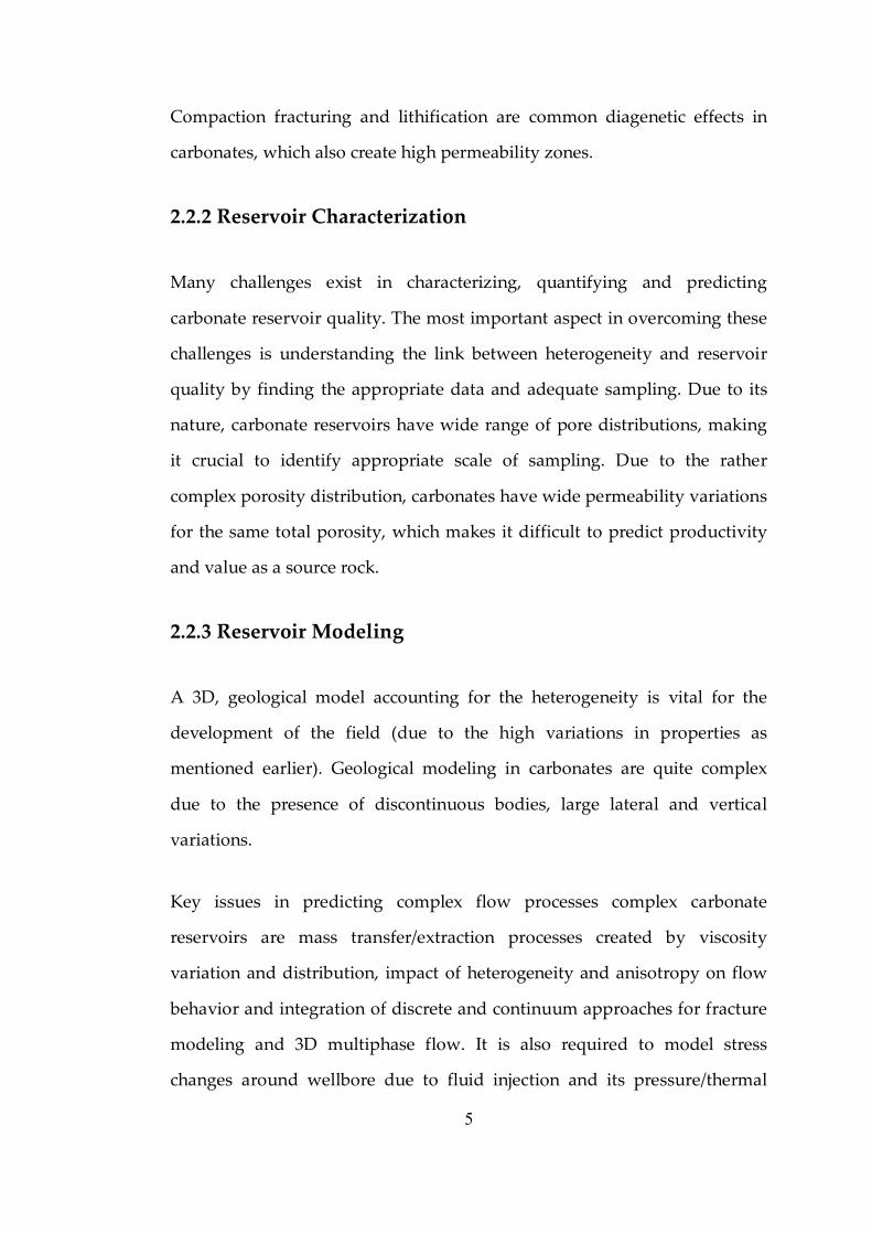
Compaction fracturing and lithification are common diagenetic effects in
carbonates, which also create high permeability zones.
2.2.2 Reservoir Characterization
Many challenges exist in characterizing, quantifying and predicting
carbonate reservoir quality. The most important aspect in overcoming these
challenges is understanding the link between heterogeneity and reservoir
quality by finding the appropriate data and adequate sampling. Due to its
nature, carbonate reservoirs have wide range of pore distributions, making
it crucial to identify appropriate scale of sampling. Due to the rather
complex porosity distribution, carbonates have wide permeability variations
for the same total porosity, which makes it difficult to predict productivity
and value as a source rock.
2.2.3 Reservoir Modeling
A 3D, geological model accounting for the heterogeneity is vital for the
development of the field (due to the high variations in properties as
mentioned earlier). Geological modeling in carbonates are quite complex
due to the presence of discontinuous bodies, large lateral and vertical
variations.
Key issues in predicting complex flow processes complex carbonate
reservoirs are mass transfer/extraction processes created by viscosity
variation and distribution, impact of heterogeneity and anisotropy on flow
behavior and integration of discrete and continuum approaches for fracture
modeling and 3D multiphase flow. It is also required to model stress
changes around wellbore due to fluid injection and its pressure/thermal
6
effects and the resulting sensitivity of the properties like permeability (Al‑
Hanai et al, 2000). Complex rock texture in carbonates produces complex
interrelationships between porosity, permeability, water and hydrocarbon
saturation and capillary. Established understanding of reservoir
connectivity issues like orientation of flow‑barriers, high permeability
streaks, vertical interconnection of layers to determine migration paths,
cross flow of fluids and gravity effects are very important. A detailed,
consistent geological model is therefore the fundamental issue in successful
reservoir management.
The prediction of permeability in heterogeneous carbonates from well‑log
data represents a difficult and complex problem. Generally, a simple
correlation between permeability and porosity cannot be developed, and
other well‑log parameters need to be embedded into the correlation.
Rahman et al (1991) studied the performance of a complex carbonate
reservoir under peripheral water injection. Study illustrated the importance
of good surveillance data for characterizing reservoirs. The available data in
that study, including well performance, geochemical analysis, cased and
openhole logs were utilized to determine water encroachment patterns,
areal and vertical sweep of the injection. Study concluded that peripheral
injection is a viable and significant option which has achieved its objective of
maintaining the reservoir pressure and sweeping the oil in the permeable
zones of the case study. With good vertical communication and favorable
mobility ratio, it is possible to achieve better flooding process.
Suryanarayana and Lahiri (1996) studied a case field in India for exploring the
issues in characterization of a complex carbonate reservoir. The field had
major hydrocarbon accumulation in the middle and lower Miocene layered
7
carbonates with shale intercalations and many wells of the field have
become underproductive due to high water cut. Characterization was
carried out by integrating petrophysical, geological, reservoir and seismic
data. Study concluded that subtle faults are the probable source for
movement of fluids in the reservoir. Further observations indicated that the
presence of cross trends of very minor faults can not be ruled out as oil
water contact within each fault block is controlled by local heterogeneities.
2.3 Geothermal Reservoirs
During the oil crisis of 1973, world suddenly became aware that fossil fiel
resources are limited and will be exhausted soon if new alternatives are not
put into use immediately. Conservation measures and extensive research on
new sources of energy has eased the demand on fossil fuelds, especially
crude oil (Okandan, 1988). Geothermal reservoir engineering emerged as an
important field in the assessment of geothermal resources.
Geothermal energy is the heat extracted from earth’s crust. When extracted
(usually in the form of hot water or steam), this energy can be utilized by
transforming heat energy to electric energy, or in local use. Different types
of resources classified according to their temperatures, will require different
energy extraction methods and uses. Reservoir engineering assessment
starts with exploration stage and continue with more importance after
power plant operation (where heat is transferred to electricity).
2.3.1 Occurrence of Geothermal Sources
There are four main requirements for a geothermal resource to be
considered as viable:

8
1) A heat source, magma body or hot dry rock at depth
2) A fluid migration which carries hot water
3) Permeable bed which will permit transmition and production of the fluid
4) A cap rock to seal the fluid migration paths and form a trap
Location of geothermal areas on the crust is dicated by global plate tectonics
and there exists six geothermal belts where most of the geothermal fields
exist (Okandan, 1988).
The biggest differentiating factor between geothermal energy and fossil
fuels is the way they are utilized. Fossil fuels are processed in plants and are
transferred through pipe lines or other means, where as geothermal energy
is utilized where it is produced.
2.3.2 Re‑injection
There are two types of geothermal reservoirs. One is the hot‑water (liquid
dominated) which produces saturated steam accompanied by large
quantities of hot water or brine; and the other is the steam, (vapor‑
dominated) system which produces steam as opposed to water.
The energy recovered from the fluids produced from geothermal systems
can be used for different purposes, mainly for electric generation. Electric
generating plants which use condensing turbines generate an excess of spent
hot liquid and condensed steam which must be discarded. Water producing
fields yield large volumes of waste water which goes through turbines and
release energy. Disposal of this waste water is generally a problem due to its
9
chemical contents and temperature. One significant solution is to reinject
waste water back into the reservoir. The term “reinjection” is often used to
describe a process where waste water is injected to the reservoir for the first
time. Reinjection is also important for optimization of a geothermal field.
(Ramey, 1981). Reinjection process serves following purposes:
Thermal energy extraction – Recovering additional heat from the system is
possible by injecting cold water to the system so that heat is extracted from
source rock.
Pressure support – As natural recharge rarely replaces the large mass of
fluid produced for power generation, injecting water in to the reservoir
compensates for the pressure decrease caused by removal of hot water for
energy generation. Especially in liquid‑dominated reservoirs this is an
important issue (Einarsson et al, 1975).
Reinjection also may affect ground subsidence in a production area. The
effect of reinjection on subsidence has been discussed by Milora and Tester
(1976).
2.3.3 Reinjection Process
The biggest consideration on reinjection is where to locate the well. The
answer to this question lies in the evaluation of the reservoir rock and fluid
properties. For a given field, both the location and flow rates of the injection
wells are important parameters effecting future performance of the field.
Here are some considerations in location selection:
10
Channeling and early breakthrough of cold liquid should be avoided. When
a high permeable channel is injected with cold water, fluid bypasses the rest
of the lower permeability zones thus reaching to producing wells faster with
minimal sweep of the area. In a study on Ahuachapan geothermal field in El
Salvador, Bodvarsson (1970) suggested that the lateral distance between two
wells shall be at least 1.1 km and the water be injected a few hundred meters
below the principal production horizons. In alignment with Chasteen (1975)
also suggested the use of an injection interval shall be deeper than the
producing interval in the adjacent producing wells.
As breakthrough of cold injected water at a discharging well causes the
produced water temperature to decrease, it is very important to forecast the
temperature at the discharging wells as a function of time to figure out the
anticipated arrival time of the cold water front.
Various theoretical studies have been carried out to investigate the effects of
reinjection on pressure maintenance in geothermal reservoirs (Lippmann et
al, 1977, Bodvarsson et al., 1985, Calore at al., 1986). These studies have shown
that injection has different effects on the reservoir response depending on
the initial thermodynamic state of the reservoir. In the case of a liquid water
reservoir the pressure effects of reinjection can readily be evaluated using
conventional analytical and numerical techniques. In cases involving two
phase liquid or vapor‑dominated reservoirs the effects of reinjection on
pressures and energy recovery are more difficult to quantify because of the
more complex physics involved (Bodvarsson and Stefansson et al, 1988).
Further complications are introduced when vapor‑only systems , where
gravity effects become dominant are investigated (Calore et al, 1986).
11
Bodvarsson et al (1985) examined the effects of reinjection in two‑phase liquid
dominated systems. They found that fluid reinjecition can cause very
pronounced increases in production rates and decreases in enthalpy.
Although injection and the associated mobility effects do not increase the
steam rate significantly in the short term, it will greatly help in maintaining
the steam rate over long periods of time. It was also pointed out that
maintaining high pressure support with acceptable low level of cooling of
the source, enthalpy recovered from the field (thus the total energy recover)
could be maximized.
Aforementioned benefits of reinjection put great emphasis on field
development stage of geothermal fields. Careful investigation of injection
location and rate plays important role in the future field performance and
therefore should be studied carefully. Reinjection of used water into the
reservoir has become increasingly common in recent years (Goyal, 1999;
Axelsson and Dong, 1998). Cost and environmental considerations are also
important factors that need to be considered for successful reinjection
process (Stefansson, 1997).
Reinjection location is arguably the most important parameter in a
successful geothermal field reinjection project. It is possible to inject water
from an outside location of the field (Einarsson et al, 1975) . A different
strategy is to inject from a location which is near the center of the field
(Bodvarsson et al, 1988) , enabling the injected water migrate towards
producing wells at a slower speed (due to a radial behavior) thus pushing
hot water to the reservoir and extracting heat from the rock. James, in 1979
suggested usage of production wells as interchangeably between production
and injection, thus reducing the cost of field development and enabling a
wider aerial sweep by spreading the injection process across the field.
12
There are also numerous studies carried on Kizildere Geothermal field (The
field used as a case study) in recent years. Arkan et al (2002) and Serpen and
Onur (2001) studied the effect of calcite scaling on pressure transient , using
Kizildere field as case study. Yeltekin et al (2002) discussed the modeling of
Kizildere geothermal reservoir. Serpen in 2002 investigated the reinjection
strategies for Kizildere geothermal field, using both in‑site and off‑site
injection strategies. They suggested producing form deeper zones and
injection to shallower parts, basing on the fact that deeper regions have
higher CO2 content. Study concluded that the most important point in
reinjection to Kizildere field is downward cooling effect of injected water
due to gravitational forces.
2.4 Optimization
As discussed briefly, petroleum engineering problems are not straight
forward, as of many real world problems. Modern reservoir models try to
combine many different types of information which are gathered from
numerous sources. Like in any problem, as the number of constraints and
parameters increase, reaching to the most feasible solution becomes more
difficult. The existence of non‑optimum solutions within the solution space
drives us to use stochastic optimization techniques.
By nature, stochastic techniques are very suitable for algorithmic
approaches. They are also effective in avoiding local solutions. The
“randomness” element of these methods provides an exit route to move
away from the local zones.
Prior to advancements in stochastic methods, more straight forward
algorithms were used to tackle optimization problems. So called “greedy”
13
algorithms like “hill climbing” were preferred for non‑linear spaces. The
chances of these algorithms to reach the global optimum are very slim.
Although they are fully “structured” searches, they do not incorporate a
way to the problem of getting stuck with local solutions.
Another batch of algorithms could be grouped as “randomized searches”.
As the name implies, in some problem specific cases (generally not too
complex), it may be possible to move towards the optimum solution by
applying a random search. This approach is not feasible for complex
problems as they do not provide a “direction” or “structure” for the search.
Stochastic methods incorporate strengths of both approaches. Although they
provide a structured search route, by combining an element of randomness,
they provide a better solution that is more likely to move towards the global
optimum. A balance between “randomness” and “structure” is deliberate.
Neural Networks (Anderson, 1995) are used as the main algorithm to
generate a proxy of the field. Usage of Neural Networks has gained
considerable popularity in the last decade. They first gained popularity as a
powerful interpolation technique and recently research is shifted towards
cognitive science. Tolerance to not exactly certain (i.e. noisy) data, ability to
respond to complex result sets are very useful for many “fuzzy” or “not
exactly defined” systems. In petroleum industry, recent research focuses on
using Neural Networks as approximate replacements for Simulations.
2.4.1 Neural Networks , Optimization and Well Placement
There are various applicatons of neural networks in the petroleum and
natural gas engineering industry. Ali in 1994 gave a synopsis of applications

14
of neural network in petroleum industry. In his study, he outlined five main
areas where neural networks are used:
1) Pattern / cluster analysis
2) Signal processing
3) Control applications
4) Predicition correlation
5) Optimization
He also points out that despite some advances on the design of optimal
network structures, it is still largely an art to determine the best paradigm.
In our study, neural networks are used for prediction correlation as a
subsystem for a supervising optimization algorithm thus combining items
four and five with the help of other techniques. His study argues the
necessity of adopting neural networks in to field of petroleum, being
influenced by the advancements and latest research that has proved the use
of neural networks as a viable tool on different aspects of industry needs.
This study incorporates neural networks as an helper algorithm to
optimization of well placement. As also pointed out by the study of Ali,
1994; this is a viable application scenario considering its main virtues:
1) Learning
2) Association ability
3) Real‑time capability
15
4) Self‑organization
5) Robustness against noise
6) Ability to generalize
(Capabilities of neural networks are described in detail in following sections
of this chapter).
There has been various studies that incorporate neural networks as a
replacement to numerical simulators or as a tool for predicting field
performance.
In 1994, Neural Networks are used as proxy of the numerical simulator in a
study to optimize groundwater remediation (Rogers and Dowla, 1994). They
used previously simulated results to train the Neural Network and there
after used it to generate decision spaces.
Also in 1994, Kumoluyi and Daltaban discussed the genereal application of
higher order neural networks inspecting various issues and application
areas. Discussing the difference between conventional neural networks
which have activation functions that are linear correlations of their inputs
and higher order networks which have a non‑linear correlation of their
inputs. Discussion was presented to be a background source for application
of networks, investigating general overview of pattern recognition,
properties of neural networks, definition of higher order neural networks
and applications of them in petroleum engineering.
In 1995 Aanonsen et al used different well configurations to train Neural
Network and used the trained system to generate decision surfaces. Those
16
surfaces are then used to estimate the well location. It was demonstrated
that Neural Networks proved successful in simple cases and the estimated
response surface was accurate enough to be used for proper location.
Following the study of Aanonsen et al, Pan and Horne (1998) used Neural
Networks along with kriging to reduce the number of simulations. Study
proposed to use some refinement areas that are of higher interest for
evaluation.
Also in 1998, Doraisamy et al studied key parameters controlling the
performance of neuro‑simulation applications in field development. They
described the use of artificial neural networks in exploring field
development strategies in conjunction with various recovery schemes. Study
focused on important neural network parameters with relevance to recovery
scenarios which have an overall objective to increase the rate of oil recovery
under specified GOR and WOR constraints. As efficiency and accuracy of an
artificial neural network are controlled by various parameters that are
specific to a given network topology, it was argued that having a robust
knowledge on those parameters are crucial for succesfull network design
and implementation.
Study was carried on three cases: In‑fill drilling where over‑training of the
neural network was investigated, Gas injection where effect of the number
of middle layer neurons on the training process was discussed and water
injection where again effect of number of middle layer neurons and the
learning constant on the training process was examined.
Study concluded that two of the more important parameters in a neural
network that control its overall performance are the learning constant and
the number of middle layer neurons. It was suggested that for studies
17
involving little or no noise, using the least possible number of middle layer
neurons resulted in a well trained network. However, in the case of wide
disparity between different scenarios, using higher number of middle layer
neurons was found to be necessary.
Farshad et al (1999) studied the “prediction” cababilities of neural networks
for tempereature profiles in producing oil wells. In the study , neural
networks were used for replacing theoretical principals such as energy,mass
and momentum balances (through regression). Study presented a novel
approach of using neural networks for predicting temperature profiles of
flowing fluid at any depth in oil wells. Farshad et al tested networks using
temperature profiles from seventeen wells in the Gulf Coast area.
In their study Farshad et al concluded that the neural network models
successfully mapped the general temperature‑profile trends of naturally
flowing oil wells. Among the tested networks, the better of the two model
predicted the fluid temperature with a mean absolute relative percentage
error of 6% where all of the networks used backpropagation algorithm for
training.
Stoisits et al (1999) used combination of Neural Networks and Genetic
Algorithms in a study for production optimization. Neural Networks were
used to represent the components of the production system.
Again in 1999, a study carried out by Centilmen et al on nonlinear effects of
well configurations used Neural Networks as a replacement for simulators.
Study demonstrated the implementation of a neuro‑simulation technique
that forms a bridge between a mathematically rigorous reservoir simulator
and neural network that uses the simulator outputs as training data sets.
18
The numerical model was replaced by the neural network which is used to
output production profiles of the wells. Centilmen et al selected various
production scenarios to generate training sets. Trained with these data sets,
neural networks are then used to predict other scenarios that were not
present in the training numerical models. All used neural networks had 1
hidden layer (details on neural networks are presented in next chapter) and
numbers of neurons for each layer were determined by the complexity of the
case. Centilmen et al grouped the input of networks into two categories;
stationary and case dependent variables. Stationary parameters were the
ones used for similar problems, such as training well locations and time.
Non‑stationary parameters were case‑specific such as distance between two
training wells, distance between existing wells and training wells, functional
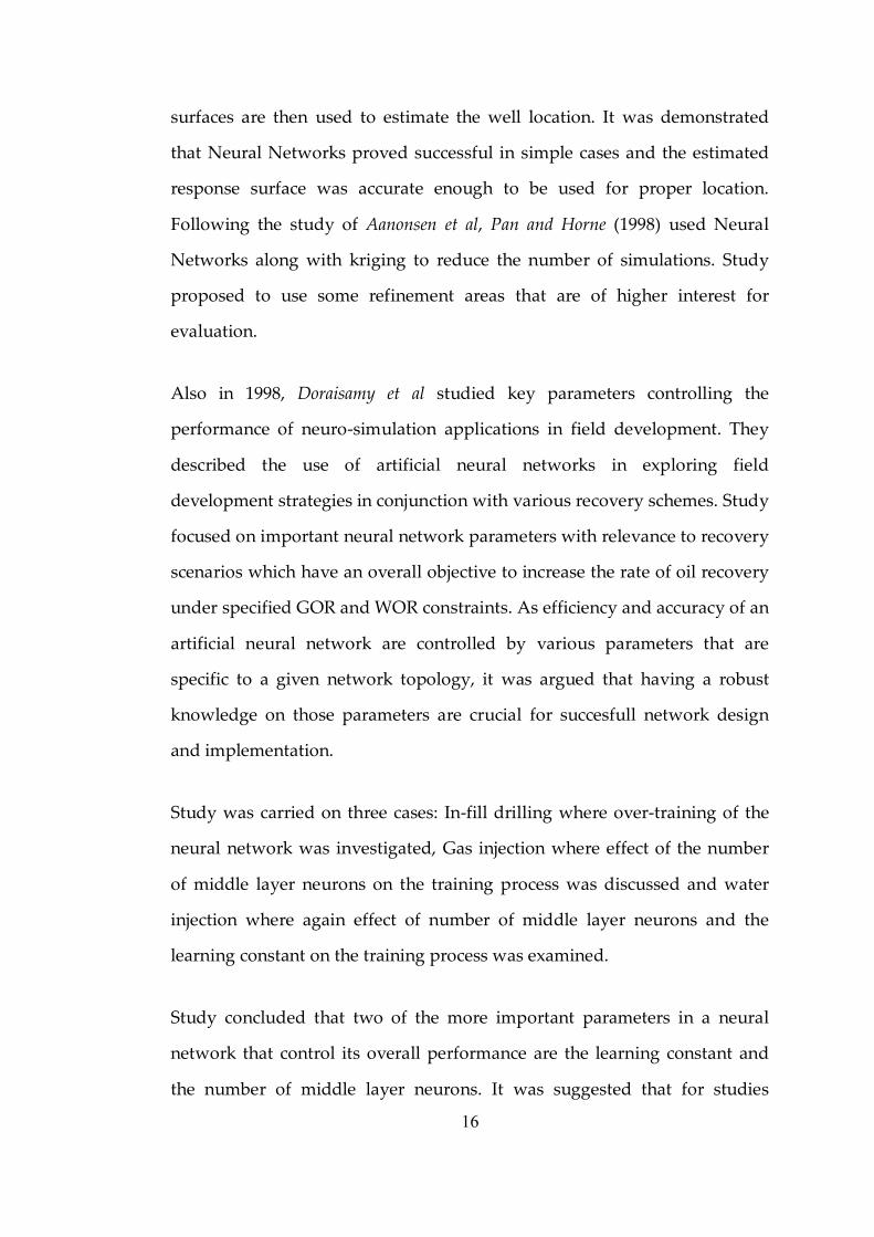
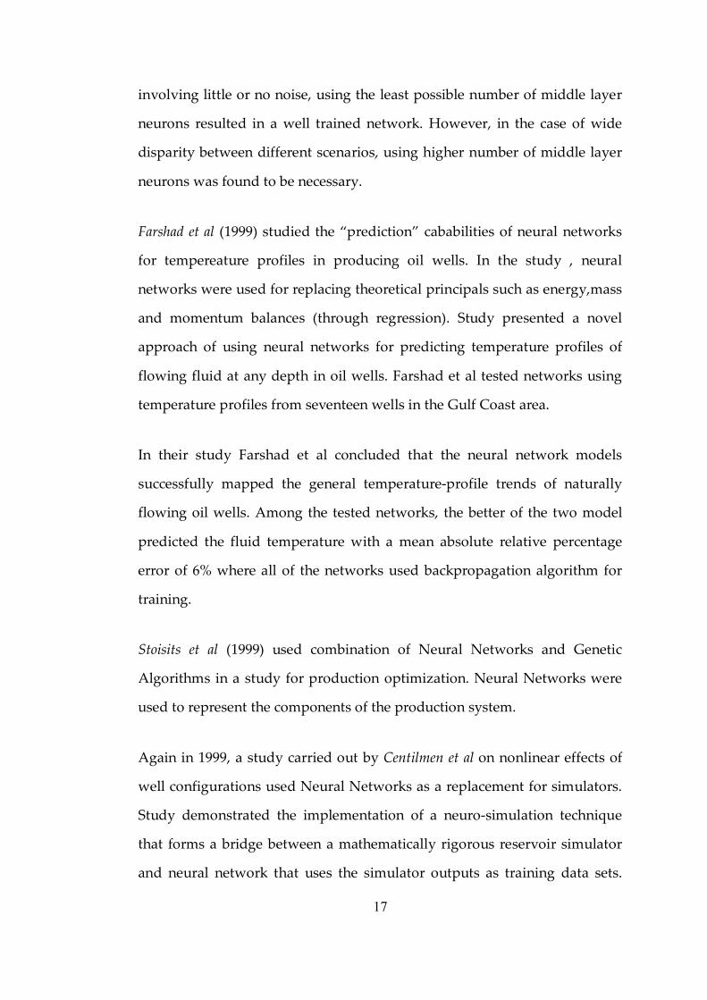
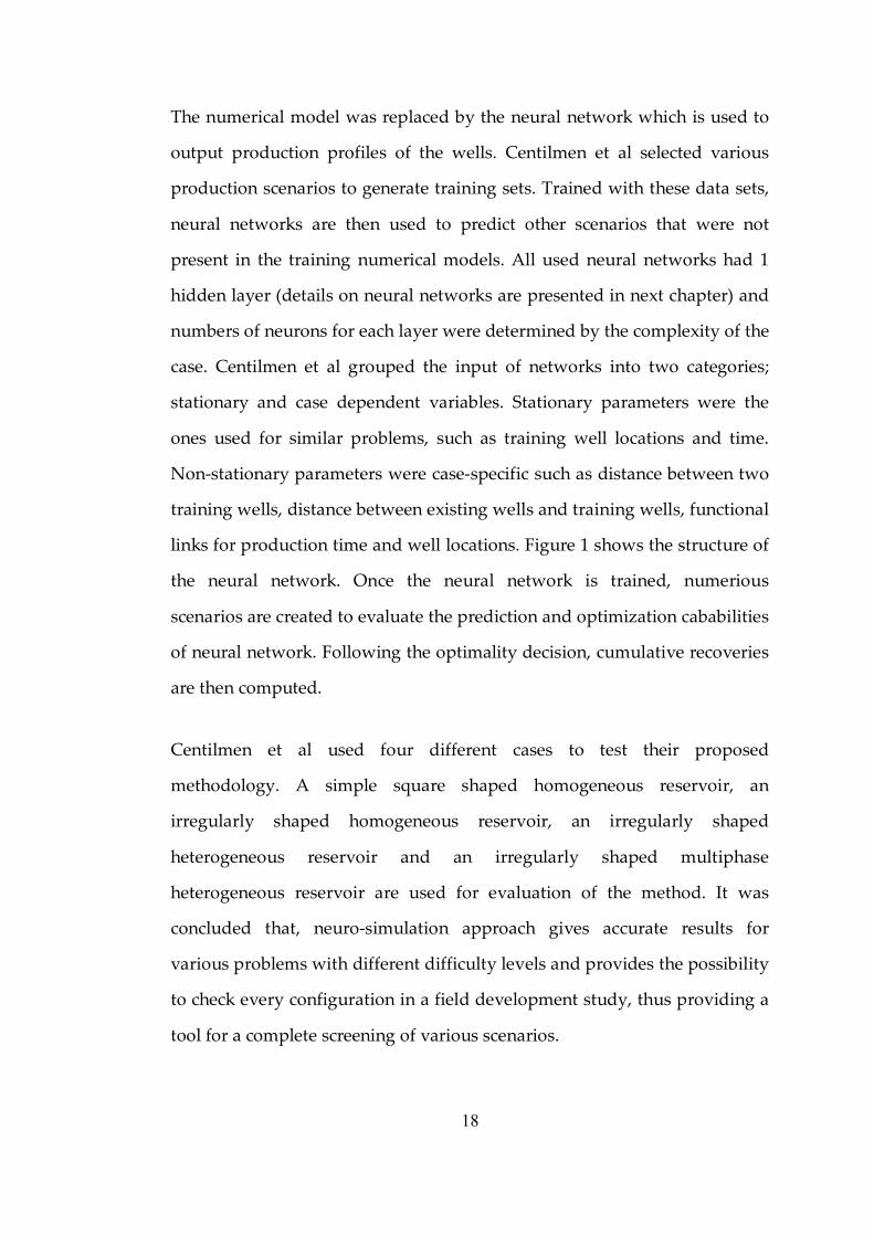
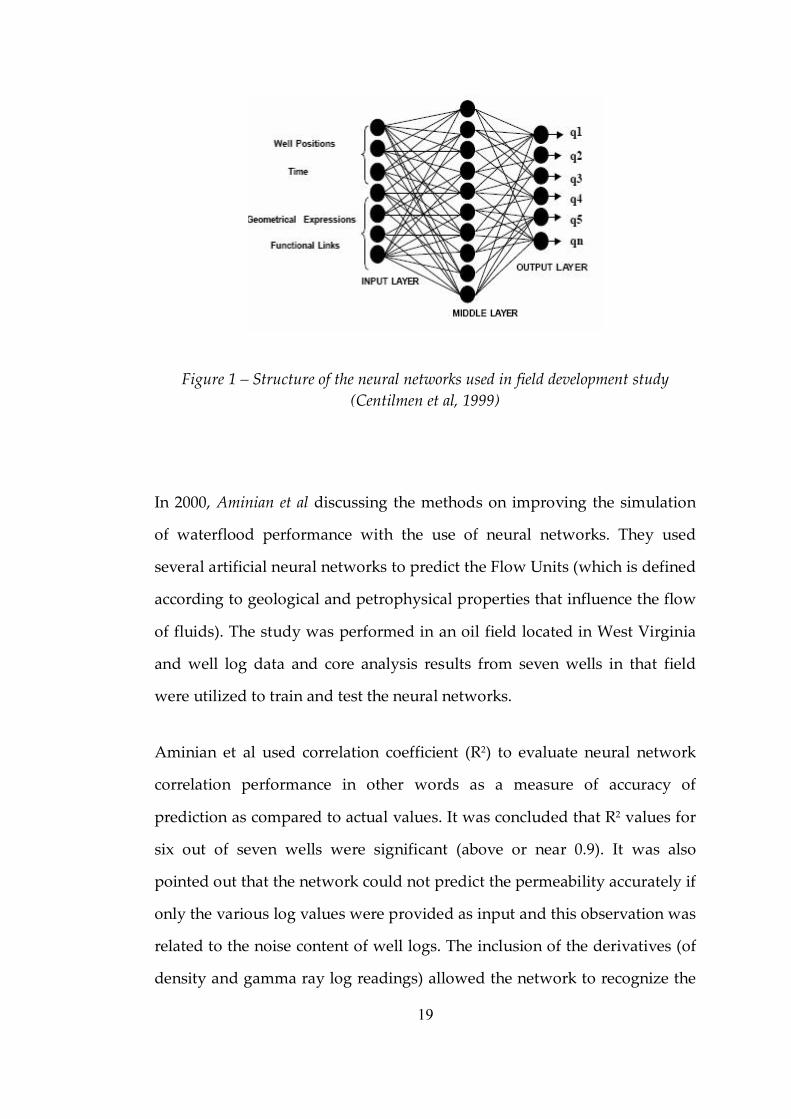
links for production time and well locations. Figure 1 shows the structure of
the neural network. Once the neural network is trained, numerious
scenarios are created to evaluate the prediction and optimization cababilities
of neural network. Following the optimality decision, cumulative recoveries
are then computed.
Centilmen et al used four different cases to test their proposed
methodology. A simple square shaped homogeneous reservoir, an
irregularly shaped homogeneous reservoir, an irregularly shaped
heterogeneous reservoir and an irregularly shaped multiphase
heterogeneous reservoir are used for evaluation of the method. It was
concluded that, neuro‑simulation approach gives accurate results for
various problems with different difficulty levels and provides the possibility
to check every configuration in a field development study, thus providing a
tool for a complete screening of various scenarios.
19
Figure 1 – Structure of the neural networks used in field development study (Centilmen et al, 1999)
In 2000, Aminian et al discussing the methods on improving the simulation
of waterflood performance with the use of neural networks. They used
several artificial neural networks to predict the Flow Units (which is defined
according to geological and petrophysical properties that influence the flow
of fluids). The study was performed in an oil field located in West Virginia
and well log data and core analysis results from seven wells in that field
were utilized to train and test the neural networks.
Aminian et al used correlation coefficient (R 2 ) to evaluate neural network
correlation performance in other words as a measure of accuracy of
prediction as compared to actual values. It was concluded that R 2 values for
six out of seven wells were significant (above or near 0.9). It was also
pointed out that the network could not predict the permeability accurately if
only the various log values were provided as input and this observation was
related to the noise content of well logs. The inclusion of the derivatives (of
density and gamma ray log readings) allowed the network to recognize the
20
changes in the shape of the various log responses, which led to a successful
neural network development. Study concluded that the neural network
predictions significantly improved the simulation of the secondary recovery
performance.
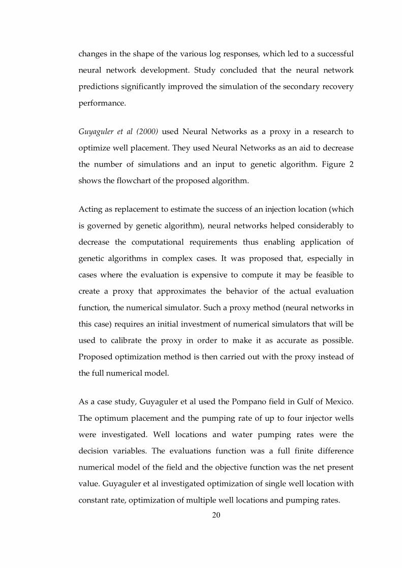
Guyaguler et al (2000) used Neural Networks as a proxy in a research to
optimize well placement. They used Neural Networks as an aid to decrease
the number of simulations and an input to genetic algorithm. Figure 2
shows the flowchart of the proposed algorithm.
Acting as replacement to estimate the success of an injection location (which
is governed by genetic algorithm), neural networks helped considerably to
decrease the computational requirements thus enabling application of
genetic algorithms in complex cases. It was proposed that, especially in
cases where the evaluation is expensive to compute it may be feasible to
create a proxy that approximates the behavior of the actual evaluation
function, the numerical simulator. Such a proxy method (neural networks in
this case) requires an initial investment of numerical simulators that will be
used to calibrate the proxy in order to make it as accurate as possible.
Proposed optimization method is then carried out with the proxy instead of
the full numerical model.
As a case study, Guyaguler et al used the Pompano field in Gulf of Mexico.
The optimum placement and the pumping rate of up to four injector wells
were investigated. Well locations and water pumping rates were the
decision variables. The evaluations function was a full finite difference
numerical model of the field and the objective function was the net present
value. Guyaguler et al investigated optimization of single well location with
constant rate, optimization of multiple well locations and pumping rates.
21
Figure 2 ‑ Flowchart of the algorithm proposed by Guyaguler et al (2002).
As conclusion, study pointed out that neural networks acting as proxy has
issues to be addressed. Most significant issue with neural networks was the
unpredictable behavior of the trained network in some cases. It was also
discussed that the benefit of using optimization algorithms, different from a
human beings, the optimization procedure is able to evaluate all the effects
of hundreds of factors in a straightforward and precise manner.
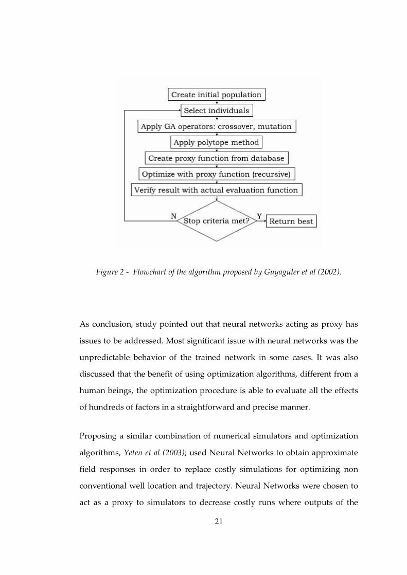
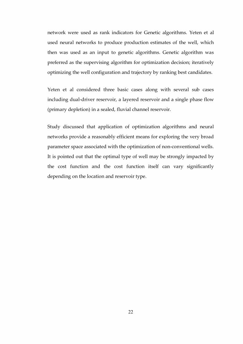
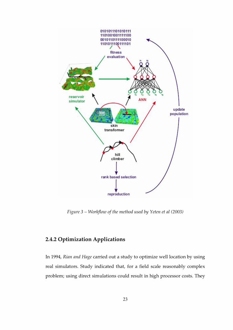
Proposing a similar combination of numerical simulators and optimization
algorithms, Yeten et al (2003); used Neural Networks to obtain approximate
field responses in order to replace costly simulations for optimizing non
conventional well location and trajectory. Neural Networks were chosen to
act as a proxy to simulators to decrease costly runs where outputs of the
22
network were used as rank indicators for Genetic algorithms. Yeten et al
used neural networks to produce production estimates of the well, which
then was used as an input to genetic algorithms. Genetic algorithm was
preferred as the supervising algorithm for optimization decision; iteratively
optimizing the well configuration and trajectory by ranking best candidates.
Yeten et al considered three basic cases along with several sub cases
including dual‑driver reservoir, a layered reservoir and a single phase flow
(primary depletion) in a sealed, fluvial channel reservoir.
Study discussed that application of optimization algorithms and neural
networks provide a reasonably efficient means for exploring the very broad
parameter space associated with the optimization of non‑conventional wells.
It is pointed out that the optimal type of well may be strongly impacted by
the cost function and the cost function itself can vary significantly
depending on the location and reservoir type.
23
Figure 3 – Workflow of the method used by Yeten et al (2003)
2.4.2 Optimization Applications
In 1994, Rian and Hage carried out a study to optimize well location by using
real simulators. Study indicated that, for a field scale reasonably complex
problem; using direct simulations could result in high processor costs. They
24
proposed a faster but limited front‑tracking simulator that is used as the
objective evaluation tool.
Simulated annealing, an optimization technique inspired from the physical
annealing process was used by Beckner and Song (1995) study. The famous
traveling salesman problem has been the basis of their approach. Beckner
and Song focused on the problem set up rather than the optimization itself.
Study concluded that optimization algorithms and numerical models could
evaluate the effects of the parameters. Their study also indicated that
optimization algorithms coupled with the numerical model has the potential
to evaluate the nonlinear effects of the optimized parameters.
In 1997, Bittencourt and Horne used a combination of Genetic algorithms and
polytope method to investigate optimization of a well placement. This
hybridized approach was used to estimate the optimum locations for 33
wells. Bittencourt and Horne proposed to use “active cells” only, pointing
out that of not used, optimization algorithm can place wells in inactive
regions. In present study, extended flow rate study somehow utilizes the
approach of active cells, focusing optimizaiton to a particular area.
Guyaguler and Gumrah (1999) studied optimization of a gas storage field by
using Genetic Algorithms to reach the optimum parameter set. Study
compared linear programming and approximate solutions and pointed
some limitations of approximate models.

25
2.5 Artificial Intelligence
2.5.1 Intelligence
Most often Artificial Intelligence (AI) is defined as the study of intelligent
behavior. This study, being mostly based on mimicking the working
principles of human brain, has been widely motivated by the the
investigation of the learning process of humans. All throughout the history,
human behavior and learning process has been a mysterious field to delve
into and many scientists have investigated the “mechanics” of human brain.
2.5.2 Artificial Intelligence
The term “Artificial Intelligence” which was mostly used in science fiction
novels during the early 20th century, has always been a dream of mankind
in one or another way. The curiosity genes of mankind coupled with the
ever improving intellectual capacity; had always asked the very same
question: “How do we learn? How do we infer?”. These two questions, in
the quest of searching the fundamentals of human intelligence, has been the
main motivation for centuries.
With the improvement of science and technology, blended with fiction,
raised another question, or challenge: “How do we imitate human
intelligence?”. This question, being the motivation in search for artificial
intelligence, even leaded to establishment of a science discipline on its own:
“Cognitive Science”. The term “Artificial” perfectly suits to its place, as the
outcome is merely the imitation of something natural (which is the basic and
vocabulary definition of the term Artificial).

26
The concept of “learning machines” has always been an interesting topic
that was well received by community as a direction of advancement.
Therefore, research towards these concepts emerged eventually.
With the significant improvement of science during past centuries, studies
on human brain have been improved and the technological advancement
enabled scientists to come with new discoveries regarding the working
principles of human brain.
2.5.3 Nero Computing
Nero computing represents general computation with the use of artificial
neural networks. An artificial neural network is a computational model that
attempts to mimic simple biological learning processes and simulate specific
functions of human nervous system. It is an adaptive, parallel information
processing system which is able to develop associations, transformations, or
mappings between objects or data. It is also the most popular machine
learning technique for pattern recognition to date. The basic elements of a
neural network are the neurons and their connection strengths (weights).
Given a topology of the network structure expressing how the neurons (the
processing elements) are connected, a learning algorithm takes an initial
model with some “prior” connection weights (usually random numbers)
and produces a final model by numerical iterations. Hence “learning”
implies the derivation of the “posterior” connection weights when a
performance criterion is matched (e.g. the mean square error is below a
certain tolerance value). Learning can be performed by “supervised” or
“unsupervised” algorithm. The former requires a set of known input‑output

27
data patterns (or training patterns), while the latter requires only the input
patterns (Russel and Norvig, 1995).
2.5.4 Human Brain
As stated before, the motivation and inspiration behind “Artificial
Intelligence” and its derivatives is human brain itself. Human brain consists
of “neurons”, which are, simply stated, electric circuit switches. Tens,
thousands of those switches come together to form “functions” of brain. All
processes from controlling our body movements to learning a new word, is
merely a process of adjustment of the setting of a particular neuron network.
Here are some facts about human brain (Mitchell, 1999)
‑ Neuron switching time ~.001 second
‑ Number of neurons ~10 10
‑ Connections per neuron ~10 4‑5
‑ Highly complex networks
‑ Parallel computation is necessary
Human brain is a massive system which has a very complex nature and is
very advanced by all means. Therefore, it is not very easy to simply create
an “artificial brain”, but it is possible to imitate at least some of the subsets
of the behaviors. This is where the use of artificial neural networks are valid.
(Mitchell,1999)

28
2. 6 Artificial Neural Networks
2.6.1 Introduction
Unlike the “organic” neural networks, which are part of a very complex
living structure; artificial neural networks are far simpler structures. Being
relatively simple mathematical structures, artificial neurons are relatively
simple concepts in the domain of mathematics. As it will be discussed
further on, although they are simple in their nature and theory, when
connected to each other (just like the real neurons in human brain) they form
a really powerful tool for wide range of applications in many different
fields. Although being different in its nature, both neural networks share the
same philosophy and analogy.
Being already explained, the “organic” neural network structure is like part
a. Part b is a model of an artificial neuron (which is connected to some other
neurons). The mathematical model (which will be discussed further on) is a
fairly simple yet powerful representation of the same functionality of
human neurons. An artificial neural network, ANN, is a structure of
interconnected neurons, forming an intelligent body on its own.
0
n
i i i
net w x =
= ∑ 1 ( )
1 net o net e
σ − = = +
Figure 4 An Artificial Neuron (formulation shall be introduced further on) (Mitchell, 1999)

29
Here are some basic properties of neural nets (ANN’s):
1) Many neuron‑like threshold switching units
2) Many weighted interconnections among units
3) Highly parallel, distributed process
4) Emphasis on tuning weights automatically
2.6.2 When to Consider Neural Networks
In recent years, neural networks have been a very important tool in various
research in very wide range of disciplines. The nature of the neural
networks enables applications if:
1) Input is high‑dimensional discrete or real‑valued
2) Output is discrete and real valued
3) Output is vector of values
4) Data is noisy
5) Form of target function is unknown
6) Human readability of results are unimportant
One of the most important features of neural networks is its ability to
“figure out” a solution even from noisy data sets. This is a very important

30
property, especially in the domain of earth sciences, where there is always
noise and imprecision.
2.6.3 An Alternative Approach to Neural Networks – Statistics
Till now, neural networks are described as replicates of human brain
functionality. This point of view, which is mainly the approach taken by
cognitive and computer scientists, tends to approach problems as “learning
processes”, similar to human learning. This definition and approach of
neural networks mostly yield to application of ANN’s in cases where human
brain functionality is imitated (like character / voice recognition, man less
car driving etc.) (Mitchell, 1999).
Although this approach is generally the “idea” behind ANN’s , in some
cases, a different explanation of neural networks seems to expand the
possible applications of ANN’s. Statistical approach to neural networks
tends to describe the behavior as parameter estimation, classification or
simple estimation problem. Neural networks are seen as perfect function
estimators, which is very useful in various difficult problems where it is
very difficult to tackle with other estimation methods.
In the statistical approach to Neural Networks, instead of approaching the
tool as a human brain replacement, the NN’s are considered to be a perfect
function estimator or classifier. In most of the statistics book that covers
neural network to some extend, it is possible to see the clear difference in
approach. Statistical approach sees neural networks as perfect function
estimators. Thus, it is true that, a two layer network is theoretically capable
of estimating any function.
31
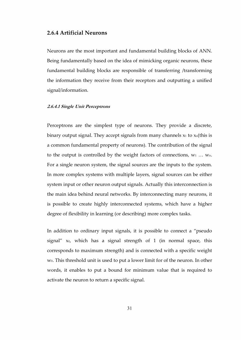
2.6.4 Artificial Neurons
Neurons are the most important and fundamental building blocks of ANN.
Being fundamentally based on the idea of mimicking organic neurons, these
fundamental building blocks are responsible of transferring /transforming
the information they receive from their receptors and outputting a unified
signal/information.
2.6.4.1 Single Unit Perceptrons
Perceptrons are the simplest type of neurons. They provide a discrete,
binary output signal. They accept signals from many channels x1 to xn(this is
a common fundamental property of neurons). The contribution of the signal
to the output is controlled by the weight factors of connections, w1 … wn.
For a single neuron system, the signal sources are the inputs to the system.
In more complex systems with multiple layers, signal sources can be either
system input or other neuron output signals. Actually this interconnection is
the main idea behind neural networks. By interconnecting many neurons, it
is possible to create highly interconnected systems, which have a higher
degree of flexibility in learning (or describing) more complex tasks.
In addition to ordinary input signals, it is possible to connect a “pseudo
signal” x0, which has a signal strength of 1 (in normal space, this
corresponds to maximum strength) and is connected with a specific weight
w0. This threshold unit is used to put a lower limit for of the neuron. In other
words, it enables to put a bound for minimum value that is required to
activate the neuron to return a specific signal.
32
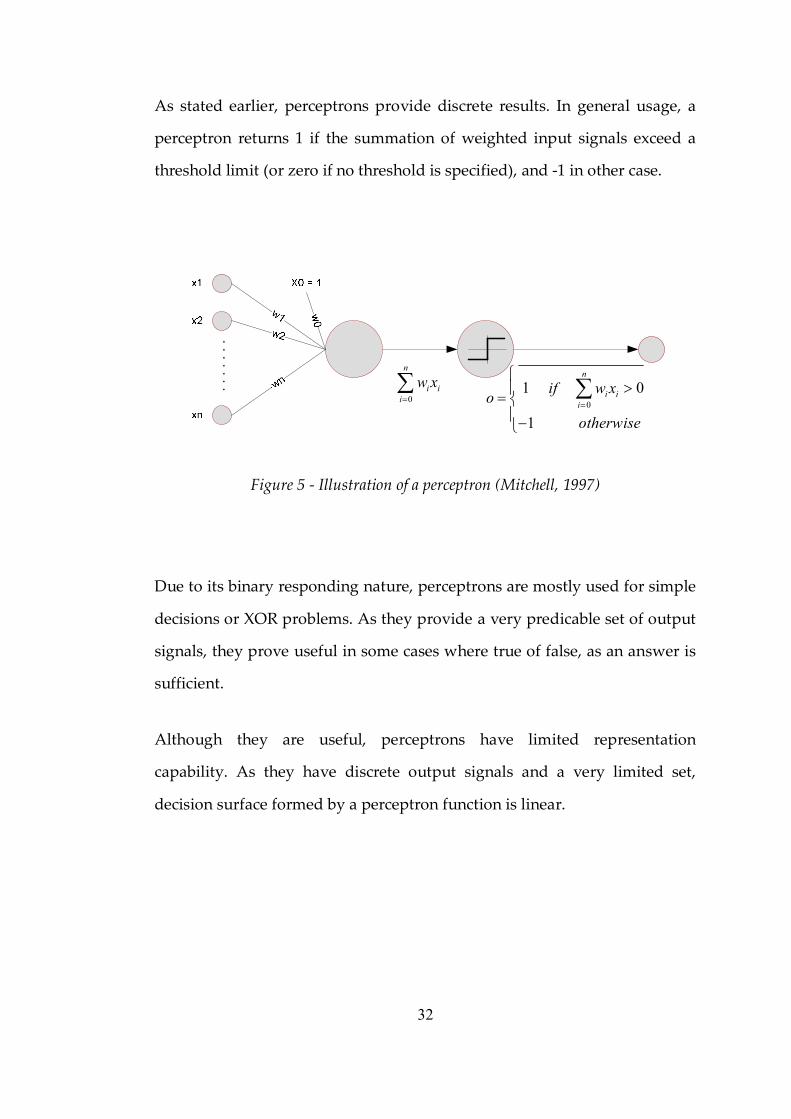
As stated earlier, perceptrons provide discrete results. In general usage, a
perceptron returns 1 if the summation of weighted input signals exceed a
threshold limit (or zero if no threshold is specified), and ‑1 in other case.
0
n
i i i
w x = ∑
0
1 0
1
n
i i i
if w x o otherwise =
> =
−
∑
Figure 5 ‑ Illustration of a perceptron (Mitchell, 1997)
Due to its binary responding nature, perceptrons are mostly used for simple
decisions or XOR problems. As they provide a very predicable set of output
signals, they prove useful in some cases where true of false, as an answer is
sufficient.
Although they are useful, perceptrons have limited representation
capability. As they have discrete output signals and a very limited set,
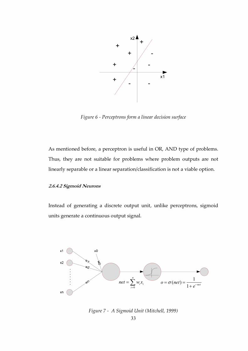
decision surface formed by a perceptron function is linear.
33
x1
x2
+
+
+
+
+
Figure 6 ‑ Perceptrons form a linear decision surface
As mentioned before, a perceptron is useful in OR, AND type of problems.
Thus, they are not suitable for problems where problem outputs are not
linearly separable or a linear separation/classification is not a viable option.
2.6.4.2 Sigmoid Neurons
Instead of generating a discrete output unit, unlike perceptrons, sigmoid
units generate a continuous output signal.
0
n
i i i
net w x =
= ∑ 1 ( )
1 net o net e
σ − = = +
Figure 7 ‑ A Sigmoid Unit (Mitchell, 1999)
34
Basic principle being the same, sigmoid units differs with their activation
function. The activation function is a transformation function that has the
net summation of all weighted signals connected to the neuron as
parameter, and a single signal as output. The important property of the
activation function is that, it has a wide mapping space, i.e. given a different
net value, it generates a unique mapping.
Although there are various activation functions, the most widely used one is
(Mitchell, 1997):
net e net
− + = 1
1 ) ( σ [1]
This activation function, which is used for our study as well, is both
computationally efficient and has an important feature such that:
)) ( 1 )( ( ) ( x x dx x d σ σ σ
− = [2]
The first order derivative is particularly important as it is used in
optimization algorithm. As having a simple, computationally efficient first
order derivative, this activation function σ(x) is advantageous in huge
networks with big training sets (which is our case). Details regarding the
usage of the first derivative will be discussed later.
2.6.4.3 Interconnected neurons – Neural Networks
The main strength of using neurons is unleashed when they are used to
create bigger systems. This is done by connecting multiple networks in
layers.

35
Inputs Outputs
Figure 8 ‑ A simple neural network with 5 inputs, one hidden layer with 2 neurons and 5 output neurons.
As illustrated in Figure 8, constructing a neural net is merely about
interconnecting the neurons. Input values then propagate in the network,
and desired number of outputs is generated by network.
Although forming a network sounds simple, design and layout of it is the
key factor for the success of the ANN. Actually the network layout is the
most important parameter that should be worked on for any ANN
application. Number of neurons in a network, the way they are connected,
number of layers they form and other similar design issues should be
successfully addressed for any successful ANN application. These issues
will be discussed in detail.
2.6.5 Learning in Neural Networks
As mentioned earlier, the fundamental concept of neural networks and
neuro computing is the learning process. Networks are used for making the
computers learn and after successfully learning the given task, applying the
gained knowledge in other samples, just like humans do.
36
Learning in neural networks is done via adjusting the contribution of signals
for each neural unit. This means that, the learning takes place with adjusting
the weights for each connection. A well trained neural network is the one
which has proper weights, which enable the network produce expected
results.
The term “learning” for a neural network actually implies the adjustment of
weights and takes place in small scale. There is no supervisor algorithm in
adjusting the weights. Each neuron is responsible for adjusting its own
weights, according to a given “training rule.
2.6.5.1 Training rule in Perceptrons
Perceptron training rule is as follows:
For each weight,
i i i w w w ∆ + ← [3]
Where
i i x o t w ) ( − = ∆ η [4]
Here, t is the target value; o is the perceptron output and η is the learning
rate (a small constant like 0.2). The learning rate one of the few parameters
that one can modify for a given network. It is used to adjust the “pace” of
the learning (Mitchell, 1999).
37
This learning rule will converge if training data is linearly separable and η is
small enough to let the training converge without over passing the best
weight update.
2.6.6 ANN Training: Search for the Best Fit
Aforementioned goal in training a Neural Net is finding the best weights
that will produce the desired outputs of the network. So the question is:
“How do we find the best weights?”. This question itself implies that we
actually have an optimization problem. We need to find the best fit (the
instance of weights that produce the most successful results over the
training set) by estimating parameters (weights). This task can be done with
different optimization methods. In our study, we choose to use Gradient
descent algorithm in training the neural network. Throughout the study, the
networks that are studied are built with sigmoid units. By doing so, we are
turning learning into an optimization problem on a continuous function (as
sigmoid units form continuous signals).
There are two steps in solving this optimization problem. The first one is
creating a continuous function (sigmoid units) and the second step is to
introduce a measure of the performance of the network which is a
continuous function of the weights and thresholds (biases). This function,
called “objective function” sets the goal for the optimization algorithm.
Although will be discussed later, it is important to mention that, in any type
of optimization, the objective function is the key element in reaching the
solution. During this study, various optimization algorithms are used in
different layers. For now, our discussion is bound with the scope of Neural
Network training.
38
The objective function used for the training for the neural network is the
sum of squared error between the target output and the produced output of
the network (Gill, Murray, Wright, 1981).
∑ ∑ − = patternp outputi
p i
p i o t E 2 ) ( [5]
So, the goal is minimizing the sum of errors between the target and
produced results. This is actually the exact approach that humans do during
a learning process. We try to get the necessary information and evaluate
ourselves according to the match of our inference with the given one.
2.6.6.1 Gradient Descent
Since the transfer function is continuous, the sum‑squared error, E, is a
continuously varying function of the weights. One way to find the “best”
weights is to find the weights which minimize the error E(W), where W
denotes the weights and biases of all of the neurons in the network. The
weights which minimize E(W) will get the network outputs as close as
possible to the desired outputs on as many patterns as possible.
Gradient descent is a general method for looking for optima of a continuous
function iteratively. The gradient of a function is a vector which points in a
direction in which that function is most increasing (most uphill). The
magnitude of the vector is related to the steepness of the slope. At optima,
the gradient is zero. If the error is a function of n weights E(w1,w2, …,wn),
then the gradient of E is a vector with n components.
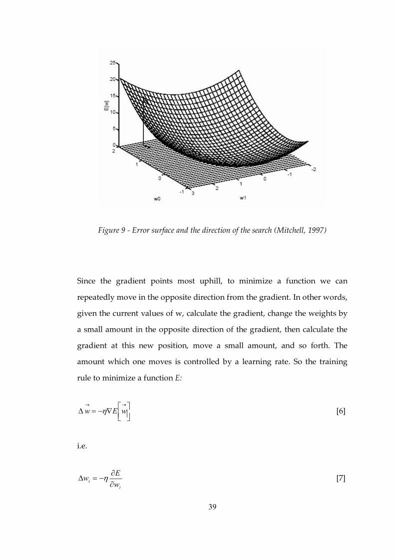
39
Figure 9 ‑ Error surface and the direction of the search (Mitchell, 1997)
Since the gradient points most uphill, to minimize a function we can
repeatedly move in the opposite direction from the gradient. In other words,
given the current values of w, calculate the gradient, change the weights by
a small amount in the opposite direction of the gradient, then calculate the
gradient at this new position, move a small amount, and so forth. The
amount which one moves is controlled by a learning rate. So the training
rule to minimize a function E:
∇ − = ∆
→ → w E w η [6]
i.e.
i i w
E w ∂ ∂
− = ∆ η [7]
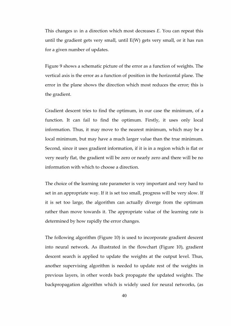
40
This changes wi in a direction which most decreases E. You can repeat this
until the gradient gets very small, until E(W) gets very small, or it has run
for a given number of updates.
Figure 9 shows a schematic picture of the error as a function of weights. The
vertical axis is the error as a function of position in the horizontal plane. The
error in the plane shows the direction which most reduces the error; this is
the gradient.
Gradient descent tries to find the optimum, in our case the minimum, of a
function. It can fail to find the optimum. Firstly, it uses only local
information. Thus, it may move to the nearest minimum, which may be a
local minimum, but may have a much larger value than the true minimum.
Second, since it uses gradient information, if it is in a region which is flat or
very nearly flat, the gradient will be zero or nearly zero and there will be no
information with which to choose a direction.
The choice of the learning rate parameter is very important and very hard to
set in an appropriate way. If it is set too small, progress will be very slow. If
it is set too large, the algorithm can actually diverge from the optimum
rather than move towards it. The appropriate value of the learning rate is
determined by how rapidly the error changes.
The following algorithm (Figure 10) is used to incorporate gradient descent
into neural network. As illustrated in the flowchart (Figure 10), gradient
descent search is applied to update the weights at the output level. Thus,
another supervising algorithm is needed to update rest of the weights in
previous layers, in other words back propagate the updated weights. The
backpropagation algorithm which is widely used for neural networks, (as
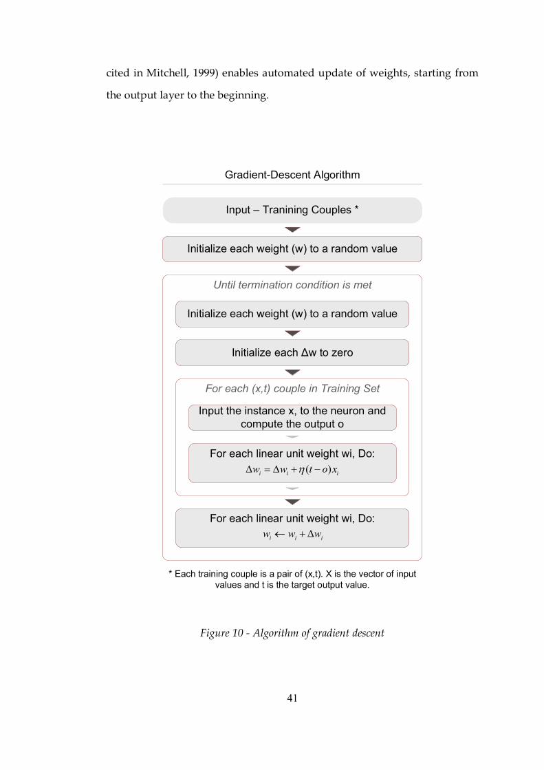
41
cited in Mitchell, 1999) enables automated update of weights, starting from
the output layer to the beginning.
Initialize each weight (w) to a random value
Input – Tranining Couples *
Until termination condition is met
Initialize each weight (w) to a random value
Initialize each Δw to zero
For each (x,t) couple in Training Set
Input the instance x, to the neuron and compute the output o
For each linear unit weight wi, Do:
For each linear unit weight wi, Do:
( ) i i i w w t o x η ∆ = ∆ + −
i i i w w w ← + ∆
GradientDescent Algorithm
* Each training couple is a pair of (x,t). X is the vector of input values and t is the target output value.
Figure 10 ‑ Algorithm of gradient descent
42
2.6.7 Backpropagation Algorithm
Being one of the most widely used algorithms for neural network training,
backpropagation algorithm (Rumelhart et al, 1986)enables a low cost weight
update scheme over complex network. The following algorithm (Figure 11)
propagates the new weight information that has been updated by gradient
descent back to the first input connections.
(1 )( ) k k k k k o o t o δ ← − −
, ,
(1 ) h h h h k k k outputs
o o w δ δ ← − ∑
, , , i j i j i j w w w ← + ∆
Figure 11 ‑ Backpropagation algorithm

43
2.6.8 Overall Training Algorithm
Following is the final algorithm for training a neural network.
1) Initialize a network with user specified number of inputs, neurons in
specified layers and outputs.
2) Initialize weights connecting the neurons (initialization is mostly done
with random weights between 0 and 1).
3) Given a set of training input, calculate the outputs.
4) Use gradient descent to retrieve new weights for output layer.
5) Use backpropagation algorithm to update rest of the weights.
6) Use the same set of inputs with the updated weights and do the steps 3‑5
recursively.
7) Stop training when the stopping criteria is met.
2.6.9 Training Sets
Neural networks need a training data set to learn. Actually, ANN’s are
mostly used to interpolate information, that is, given a set of samples, ANN
is used to act as a proxy and approximate results given another set of input
for the same problem.
Neural networks are powerful tools for replacing forward models,
especially of those which are known to be governed according to consistent

44
equations (Caers, 2004). A wide usage of ANN’s in scientific problems is as
follows:
Given a problem, and a known solution (mostly with CPU demanding and
sometimes difficult to calculate analytical solution) a set of results are
calculated or if applicable, experimental results are collected.
Then, a Neural Network is trained to learn the behavior that is governed
with the equations. As using a trained ANN is far less costly than doing
equation calculations, or say running simulators, afterwards, Neural
Network is used in replacement.
The above mentioned methodology indicates a critical point: The training
set is the only bridge between the real case and the neural network and
therefore it should be as healthy as possible.
As mentioned earlier, ANN’s are not very sensitive to noises and are very
good at inferring results from noisy data (Mitchell, 1997; Caers 2004). This
property is probably that makes a neural network a good option in
deducing results from “observation” type of problems (like experiment
results). The term “healthy” used in the previous paragraph does not refer
to the “precision” of the training set, but rather the way it is subdivided.
For training a neural network, it is required to have 3 groups of data sets
which are gathered from exactly the same source in same conditions. In
other words, when we are given a data set, we will need to divide it into
three sub groups. The reason we use three groups and their usage is as
follows:

45
The first group, training set, is the one that will be used to train the neural
network. It is be used in the aforementioned iterative training process.
Second set, the evaluation set, is be used to evaluate the network during the
training. In other words, after each training iteration, the exact network
snapshot is used to calculate the error of that particular shot and recorded. It
should be noted that, the calculation of weights and backpropagation of
updated values are done for the training set, evaluation set is only used for
the forward pass. Same evaluation set may be used to evaluate the trained
network (or this set may be sub divided into two to keep some part of it for
post evaluation).
The third set is the one that is never shown to the network before it gets past
the training stage. This set is used to make sure that the trained Neural
Network acts as expected even for data sets it has never seen.
2.6.10 Stopping Criteria in Neural Network Training
2.6.10.1 Stopping Criteria in Optimization
In any optimization problem, one needs to define a stopping criterion to end
the iterative process for searching the “best fit”. One might argue about the
reason why it would be viable to stop before reaching the ultimate target,
the exact match. The simple reason is that, in most of the cases, the exact
match is impossible to reach. More importantly, it may be very costly to
reach the fit, whereas we can obtain a “good enough” fit with far less
iterations. In most of the iterative optimization algorithms and specially in
derivative using methods like Gradient Descent or Newton’s method and its
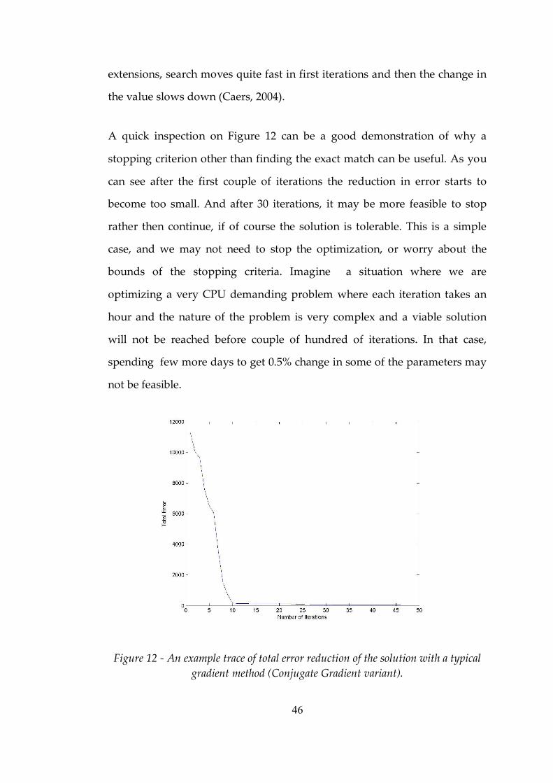
46
extensions, search moves quite fast in first iterations and then the change in
the value slows down (Caers, 2004).
A quick inspection on Figure 12 can be a good demonstration of why a
stopping criterion other than finding the exact match can be useful. As you
can see after the first couple of iterations the reduction in error starts to
become too small. And after 30 iterations, it may be more feasible to stop
rather then continue, if of course the solution is tolerable. This is a simple
case, and we may not need to stop the optimization, or worry about the
bounds of the stopping criteria. Imagine a situation where we are
optimizing a very CPU demanding problem where each iteration takes an
hour and the nature of the problem is very complex and a viable solution
will not be reached before couple of hundred of iterations. In that case,
spending few more days to get 0.5% change in some of the parameters may
not be feasible.
Figure 12 ‑ An example trace of total error reduction of the solution with a typical gradient method (Conjugate Gradient variant).

47
2.6.10.2 Overfitting (Memorization) Problem in Neural Networks
As mentioned earlier, training a neural network can be seen as an
optimization problem. We have to deal with the same issue of finding the
best cut off criteria. In neural network training, this cut off point has even
more importance than an ordinary optimization problem (Mitchell, 1997).
2.6.11 Design Issues in Neural Networks
As mentioned before, it is possible to create infinite number of different
network designs that may address the very same problem. Although there
are no “mathematically exact” tools to calculate the success of a particular
network design for a specific problem, some general guidelines exists to
assist in finding a reasonable network design for a problem.
2.6.11.1 Effect of Number of Neurons and Layers
The number of layers of a network does have a calculateable impact on the
representation power of the neural networks.
Recalling from the statistical approach to ANN’s, if networks are treated as
classifiers or discriminating boundaries, it is visually possible to explain the
impact of having different number of layers and nodes.

48
Figure 13 ‑ Discriminants made by Multi‑layer neurons with different number of layers (Caers, J., 2004)
As you can see, a one layer neuron makes linear discriminants, a two‑layer
network can form discriminants with a convex region and a three‑layer
network can form arbitrary discriminants.
One should note that, although increasing the number of layers do increase
the representation power of the network, same does not always hold for the
number of neurons in a layers. To give an example, in a 1 hidden layer
network, increasing the number of hidden nodes from 5 to 15 does not mean
that the later network will be more successful. This optimality should be
carried with trial and error approach.
49
2.8 Optimization
2.8.1 Introduction
Optimization theory has applications in may fields. Every decision is based
on a somehow optimized decision in any case. In petroleum engineering
practice, optimum solutions are even more important. Generally, decisions
are bound to multi million or billion results and can influence the success of
the project dramatically (Gill, Murray, Wright, 1981).
Each optimization problem has a set of goals, i.e. “the optimum target” that
is desired solution. In numerical problems generally the result is a “surface”
of solutions that represents the results obtained with different values of the
set of parameters that are being optimized. This surface can have multiple
dimensions and vary in complexity in correlation with the number of
parameters.
There are numerous algorithms to locate the optimum location over that
surface. In this study, Simplex (polytope) algorithm is used. It is a well
known algorithm, especially for its fast convergence to the maxima.
2.8.2 Simplex Algorithm
2.8.2.1 Introduction
Generally, in most of the optimization problems, the domain of interest and
the task of optimization is usually very sparse or not very well defined.
Also, in most cases, the optimization problem itself is quite complex and
speed is a constraint. Polytope (Simplex) algorithm, having its root taken
50
from graph theory, is based on a simple but very powerful algorithm. Being
a downhill algorithm just like descent ones, it is far more intelligent and
with the help of geometric approach, more efficient. (Caers, 2004, Nelder &
Mead, 1965)
2.8.2.2 The Algorithm
The polytope algorithm is as follows.
Initially, 3 points are guessed and evaluated with the objective function.
Then, they are ranked according to the value of the objective function.
Centroid of the formed triangle is calculated. (xc)
A reflection of the best point so far is taken , xc being the reflection point.
The new location, xcandid is then evaluated. According to evaluation, one of
the four possible actions are taken:
If xcandid has a better evaluation value than the worst point but less than the
best, then replace the worst point with the new one and essentially form a
new triangle which has better areal coverage of “more probable candidates”.
If xcandid has a better evaluation value than the best ranked point, then this is
very good, it means that we are in the right direction. As we prefer to move
in this direction, we actually try to expand our candidate point:
We expand the new point according to the formula:
xe: c + B(xcandid – c) where B is the expansion coefficient , c is the centroid

51
If the new expanded point is better than our candidate point, then xr
replaces the worst point.
If the new expanded point is worse than the candidate point, than the
expansion process fails and candidate point replaces the worst point in our
triangle.
If xcandid has worse evaluation value than the some of the point in our
triangle, then it means that actually our polytope is large and we want to
make it smaller so that we can approach to the solution. For that reason, we
do a contraction operation.
If xcandid is better than the worst point, then contraction point is found with:
xc=c + A(xworst – c), where A is the contraction coefficient and c is the centroid
If xcandid is worse than the worst point, then the contraction is done as: xc=c
+ A(xcandid – c).
52
CHAPTER 3
PROBLEM STATEMENT
This study focuses on development of a modern framework to optimize
injection well location in complex carbonate reservoirs. Introduced
framework utilizes neural networks and exhaustive search with stepping to
locate injection wells in a given complex carbonate reservoir.
Location of injection well is a dominant parameter in application of recovery
technique for a given field. By nature, most carbonate reservoirs have
complex structures that influence production and recovery from the field
significantly. When considering injection of waste water to a geothermal
field or injection of water in to an oil field residing in a complex carbonate
sutructure, choice of injection location plays an important role in
determining future recovery from the field.
When considering well placement for a reservoir, choices are virtually
limitless. With limited engineering and processing power, it is generally not
possible to try every option and alternative to choose the best possible
location. Engineering intuition plays an important role in eliminating
fraction of the possible choices, yet most of the alternatives are eliminated
due to lack of time and processing power. Development of a modern
approach that automates the process and reduces the processing demand is
therefore very important. This study focuses on introduction and
deployment of a framework that automates the optimization process
meanwhile keeping processing needs minimal.
53
CHAPTER 4
MOTIVATION
To provide a robust optimization solution, a general framework should be
delivered. The framework should successfully address:
Capability to avoid local optimums In any optimization problem, the most
challenging task is to overcome the problem of local solutions (Caers, 2004).
A relatively complex decision surface has more than one local solutions
which may be difficult to avoid. If algorithm is not capable of avoiding these
“local” solutions, it may be impossible to obtain the global optimum, the
ultimate solution that is desired. A capable framework should provide
necessary algorithms to overcome this.
Not being an overburden itself One of the biggest problems in
development of new numerical / algorithmic solutions to modern
engineering problems is the cost of the approach itself. In other words, if the
developed framework does not provide a far superior benefit in decreasing
the processing cost when compared to the base approaches; then it will not
be practical to use it.
Not being problem specific By definition, a “framework” should be a set of
operation, a methodology to reach a solution. Framework should be general,
so that it is problem specific and can be applied to reasonably different
problems as well.
Main motivation for this study has been to develop and study a
“framework” that is capable of addressing a well defined engineering

54
problem and provide a set of tools that can be used in different problems of
same type. Tools that are chosen as the building blocks for this framework
will be discussed in following chapters.
4.2 Basis of the Approach
Prior to the years of rapid advancement in computer technologies; reservoir
management was mostly based on intuitive decisions and expertise of
decision makers. The fact of not having enough data and the inability of
representing it accurately or lack in tools to handle it; the models developed
and used in early days lacked the resolution of detail for successfully
dealing with complex problems. With the introduction of Reservoir
Simulators and the parallel advancement in computers; resulted more
advanced predictive tools and well defined reservoir models emerged.
Increasing the accuracy and value of fields, increase in detail also resulted in
more “structured” solution models as input data exceed the limits of
“intuitive inference”.
As reservoir models incorporate more data, simulation complexity and
CPU demand increases exponentially. As of today; with the help of
supercomputers that has hundreds of processing units, companies are able
to simulate, rarely, topping approximately million grid blocks. The real cost
of running simulations are therefore important. Ideally; it would be the
ultimate goal to run hundreds of simulations to get a better understanding
of different development strategies; but this is merely impossible to tackle,
as the number of variables and the produced space of uncertainty is not
possible to define even with many simulations. The main bottle necks in
looking for the “most valuable” decision are:
55
Time constraints. Running simulations is costly and time demanding. It is
not possible to afford exhaustive run for each different possibility as
deadlines are always “too soon”.
Excessive amount of information generation. Even it is possible to run
exhaustive simulations to study the effect in change in variables, generated
set of results may be difficult to interpret and time consuming as well.
During the rather short history of modern computers, being inspired by
science fiction novels, constant research efforts has been put on building
“intelligent” systems that can deduce like a normal human. Efforts of
computer scientists resulted in various established methodologies like
neural networks, genetic algorithms, fuzzy systems, expert systems etc. and
the research is forging. Current research is based on improvement on these
fundamental theories, their applications and “fresh ideas” in the world of
artificial intelligence.
This study focuses on the application of those fresh ideas in the domain of
reservoir engineering. The developed concept and the software package,
which will be introduced briefly, aims to couple some latest advancements
in computer science over the solutions in the field of earth
science/petroleum engineering discipline.
56
CHAPTER 5
SOFTWARE IMPLEMENTATION
5.1 Software Implementation
Software implementation is an important aspect of this study as there is no
tool that is capable of handling such different algorithms to run as
integrated.
This study uses numerous advanced algorithms to tackle a specific problem
in earth sciences domain. As it will be introduced later on, development of
specific software that should integrate with other tools and use numerous
algorithms automatically, it was necessary to approach the problem as a
software development task.
5.2 Artificial Intelligence Workbench
Following chapter introduces the reader to the developed software package,
named “Artificial Intelligence Workbench” and supportive tools such as text
processors and converter modules used for retrieving high volumes of data
from simulators. Executable of the software is provided on a Compact disk
media enclosed to this thesis. Appendix A covers the necessary steps to
install the software package.
5.2.1 Overview
The tool named Artificial Intelligence Workbench is full of some attractive
features:

57
It is developed for Java 2 platform, enabling deployment to any platform.
1) Uses advanced graphical user interface
2) Uses platform independent property file format
3) Incorporates some of the recent elements of user interface tools
4) Installable via web / digital media
Figure 14 ‑ The welcome screen of Artificial Intelligence Workbench
When launched an empty workbench the welcome screen (Figure 14) is
displayed . Workbench consists of two views:
‑ Training Perspective

58
‑ Execution Perspective
5.2.2 Training Perspective
Training perspective is used for launching windows for creating new neural
network design (backpropagation for time being) and Automated Nero
Fuzzy Inference System. A separate input file creation dialog is presented as
well.
Figure 15 ‑ Network Design Window
After the design of the network, a training window is launched (Figure 15).

59
Figure 16 ‑ Training session is run with different learning rates and momentum
Training window (Figure 16) enables setting the learning rate, number of
epochs, momentum, input file and already designed network layout. The
training is initiated with the “Start” button. When a snapshot of the current
network situation is desired, “Snapshot” button can be used. Program saves
the current state of the network to a permanent file. This may be particularly
useful in altering the learning rate and momentum during the training
process.
After the training is finished (reached the desired number of iterations or
error percentage), the network state is saved.

60
5.2.3 Execution Perspective
Execution perspective is used for loading the trained network and feeding
with input data.
5.3 Software Validation
Prior to actually using the software, each module is validated so to make
sure the actual results are reliable and free of software malfunction.
5.3.1 Neural Network
For testing purposes, a sample network is designed with design window, for
simple number recognition. A matrix of size 5x5 is used for placing 0 and 1
that form a number. Figure 17 shows an example training input of number
“0”. The network had 25 input values, 5 hidden nodes in 1 hidden layer and
9 outputs and it was trained for 1000 iterations.
1 1 1 1 1 1 0 0 0 1 1 0 0 0 1 1 0 0 0 1 1 1 1 1 1
Figure 17 ‑ Binary bitmap example
The trained network responded just like expected. Numbers like “1” were
identified with a %95 success. When an input of number “8” is fed to the
trained network, outputs for “0”, “6” and “9” also gave some signal. This is
due to the similarity of those numbers when written to a 5x5 matrix.
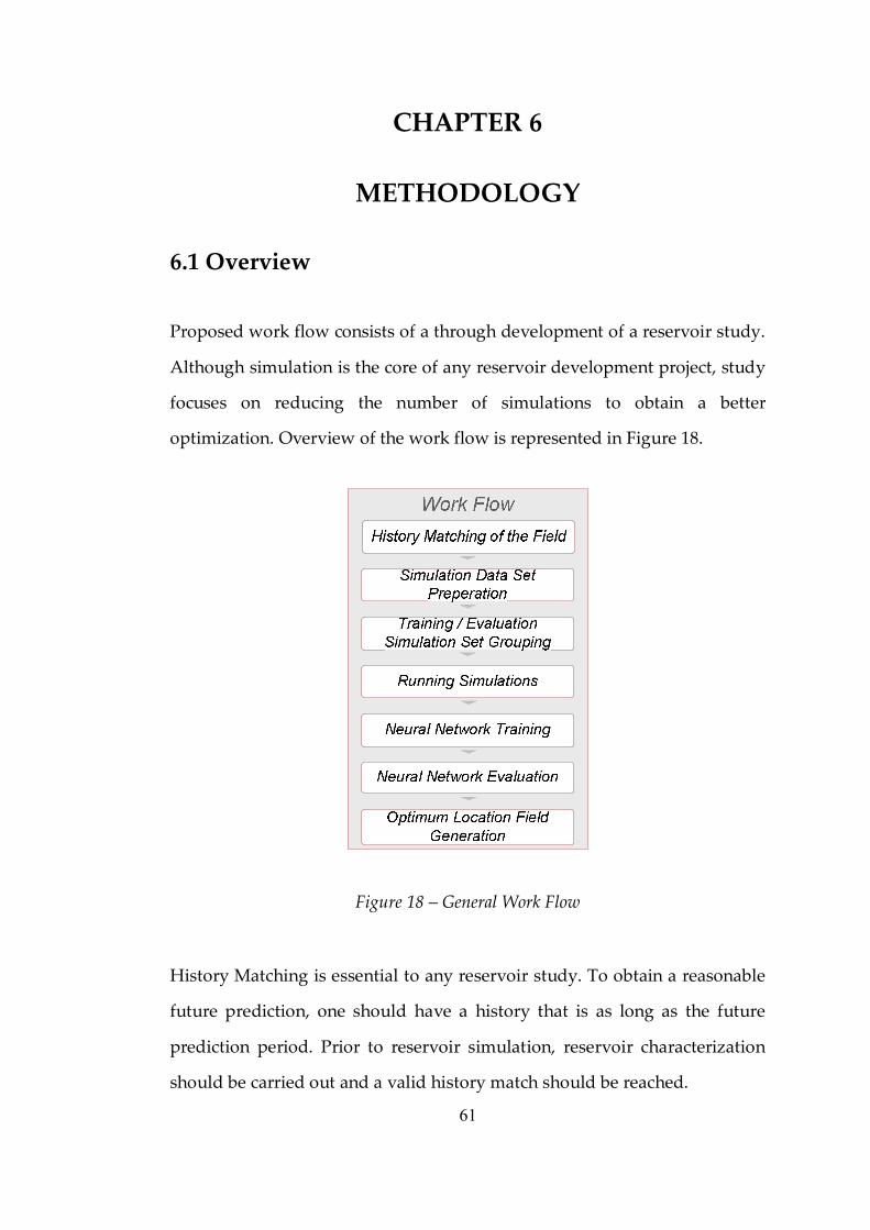
61
CHAPTER 6
METHODOLOGY
6.1 Overview
Proposed work flow consists of a through development of a reservoir study.
Although simulation is the core of any reservoir development project, study
focuses on reducing the number of simulations to obtain a better
optimization. Overview of the work flow is represented in Figure 18.
Figure 18 – General Work Flow
History Matching is essential to any reservoir study. To obtain a reasonable
future prediction, one should have a history that is as long as the future
prediction period. Prior to reservoir simulation, reservoir characterization
should be carried out and a valid history match should be reached.

62
6.2 Data Generation
A considerable time of the study is devoted to the preparation of data sets
that shall be used in the software. The process consisted of several steps:
1) Valid data collection from a real field
2) History matching of available data with simulation software
3) Creation of initial data files
4) Running the simulations
5) Collecting and modifying the result sets
6) Creating the training files
6.2.1 Valid Data Collection from the Field
As a case study, a geothermal field in Turkey, Kızıldere field, is chosen.
Figure 16 shows the top view of the field. There are 11 operational wells
drilled in various positions. (Yeltekin et al, 2002)
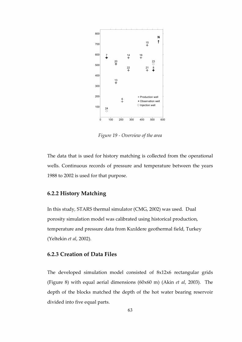
63
13
14
15
16
20
21 22
23
24
6
7
8
0 100 200 300 400 500 600
100
200
300
400
500
600
700
800
+ Production well + Observation well Injection well
N
Figure 19 ‑ Overview of the area
The data that is used for history matching is collected from the operational
wells. Continuous records of pressure and temperature between the years
1988 to 2002 is used for that purpose.
6.2.2 History Matching
In this study, STARS thermal simulator (CMG, 2002) was used. Dual
porosity simulation model was calibrated using historical production,
temperature and pressure data from Kızıldere geothermal field, Turkey
(Yeltekin et al, 2002).
6.2.3 Creation of Data Files
The developed simulation model consisted of 8x12x6 rectangular grids
(Figure 8) with equal aerial dimensions (60x60 m) (Akin et al, 2003). The
depth of the blocks matched the depth of the hot water bearing reservoir
divided into five equal parts.
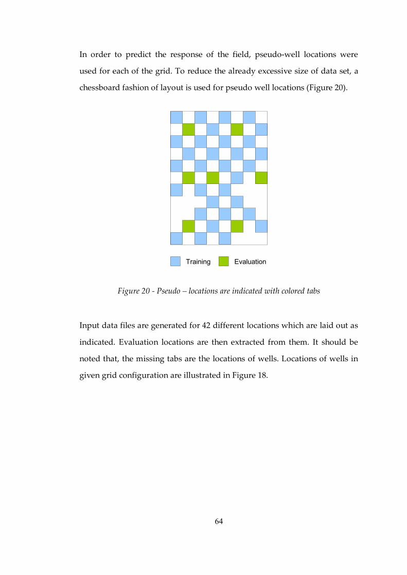
64
In order to predict the response of the field, pseudo‑well locations were
used for each of the grid. To reduce the already excessive size of data set, a
chessboard fashion of layout is used for pseudo well locations (Figure 20).
Evaluation Training
Figure 20 ‑ Pseudo – locations are indicated with colored tabs
Input data files are generated for 42 different locations which are laid out as
indicated. Evaluation locations are then extracted from them. It should be
noted that, the missing tabs are the locations of wells. Locations of wells in
given grid configuration are illustrated in Figure 18.

65
Figure 21‑ Locations of Current Wells in the Field of Study
6.2.3.1 Running the Simulations
As a CPU intensive process, each simulation run took considerable time to
finish. It took approximately 10‑20 minute to get the results for a single
simulation. As total of 42 runs were done, some important time is spent on
this phase. Resulting data set was approximately 4 Gigabytes in size, with
more than 100000 lines of data regarding the pressure and temperature
values of 11 wells. Considering the relatively small size of the field, these
figures indicate the necessity of finding reliable methods to reduce the
amount of data to be processed.
6.2.3.2 Exporting the Pressure & Temperature Values
CMG Simulation suite uses 2 different components to export Temperature &
Pressure values. Interestingly, exporting from these two different tools
results in completely incompatible files. To tackle this problem an
intermediate program, CMGConverter, is developed. This tool searches the
66
Temperature file (in which the Temperature of each grid is grouped in time
basis) and Pressure file (Pressure for each well is recorded against location)
and finds the matching time labels. When appropriate match is found, it
collects the temperature and pressure values from the files and writes to a
new file which is Excel compatible.
6.2.4 Creating Training Input Files
To decrease the size of the data sets and prepare for time unfolding
approach which requires constant time intervals, the exported and
combined files needed to be further refined. For that purpose, 3 Excel
macros have been written. These macros initially select the equal time step
values (data record line for 5 th of each month) and create separate files
containing only these lines. This processing decreased the data record lines
from 3500+ to 119. As the change in time and pressure values are
continuous and non‑fluctuating, this refinement in not expected to produce
any loss of information.
67
CHAPTER 7
RESULTS AND DISCUSSION
Afore mentioned algorithms and developed software package is studied in a
real life case study. This chapter introduces the nature of the discussion and
the observations regarding the application of theory.
7.1 Field of Study
7.1.1 Introduction
A Geothermal field located in Kızıldere, Turkey is chosen as the field of
study. Although there are some different constraints by nature of the
problem; algorithmically theory is applicable to any simulation tailed
problem regarding underground fluid flow. The only difference between
different types of fluid flow is the “objective function” used to evaluate what
is “good” and “bad” regarding field performance.
7.1.2 Simulation Model
In this study, STARS thermal simulator (CMG, 2002) was used. Dual
porosity simulation model was calibrated using historical production,
temperature and pressure data from Kızıldere geothermal field, Turkey
(Yeltekin et al, 2002). The simulation model (Akin et al, 2003) (Table 1)
consisted of 8x12x6 rectangular grids with equal areal dimensions (60x60
m). The depth of the blocks matched the depth of the producing reservoir
(Igdecik formation) divided into five equal parts. Figure 22 shows the grid
tops of the producing layer. The last z block was thick (5000 m) and was
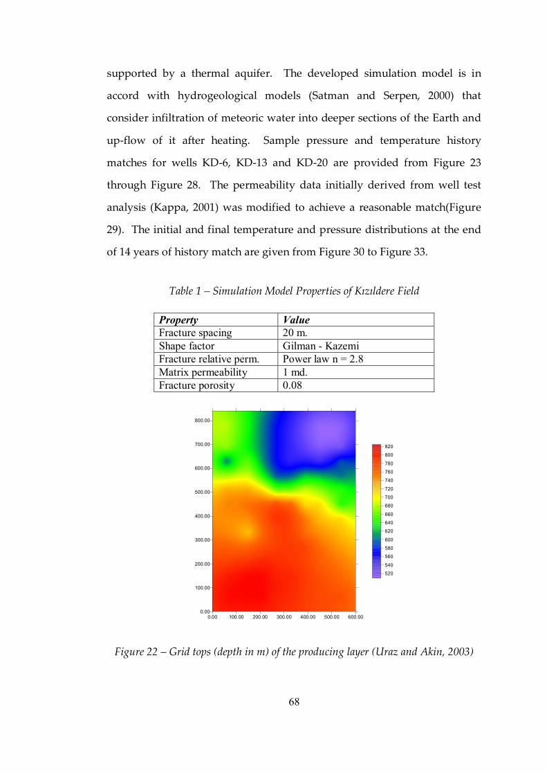
68
supported by a thermal aquifer. The developed simulation model is in
accord with hydrogeological models (Satman and Serpen, 2000) that
consider infiltration of meteoric water into deeper sections of the Earth and
up‑flow of it after heating. Sample pressure and temperature history
matches for wells KD‑6, KD‑13 and KD‑20 are provided from Figure 23
through Figure 28. The permeability data initially derived from well test
analysis (Kappa, 2001) was modified to achieve a reasonable match(Figure
29). The initial and final temperature and pressure distributions at the end
of 14 years of history match are given from Figure 30 to Figure 33.
Table 1 – Simulation Model Properties of Kızıldere Field
Property Value Fracture spacing 20 m. Shape factor Gilman Kazemi Fracture relative perm. Power law n = 2.8 Matrix permeability 1 md. Fracture porosity 0.08
0.00 100.00 200.00 300.00 400.00 500.00 600.00 0.00
100.00
200.00
300.00
400.00
500.00
600.00
700.00
800.00
520
540
560
580
600
620
640
660
680
700
720
740
760
780
800
820
Figure 22 – Grid tops (depth in m) of the producing layer (Uraz and Akin, 2003)
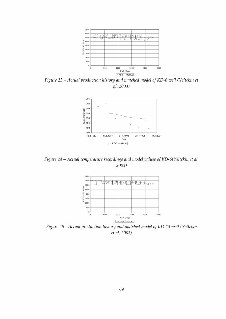
69
0
1000
2000
3000
4000
5000
6000
7000
8000
9000
0 1000 2000 3000 4000 5000
TIME (Day)
PRESSURE (kPa)
KD6 MODEL
Figure 23 – Actual production history and matched model of KD‑6 well (Yeltekin et al, 2003)
190
192
194
196
198
200
202
204
18.2.1982 11.8.1987 31.1.1993 24.7.1998 14.1.2004
Date
Temperature (C
)
KD6 Model
Figure 24 – Actual temperature recordings and model values of KD‑6(Yeltekin et al, 2003)
0
1000
2000
3000
4000
5000
6000
7000
8000
0 1000 2000 3000 4000 5000
TIME (Day)
PRESSURE (kPa)
KD13 MODEL
Figure 25 ‑ Actual production history and matched model of KD‑13 well (Yeltekin et al, 2003)
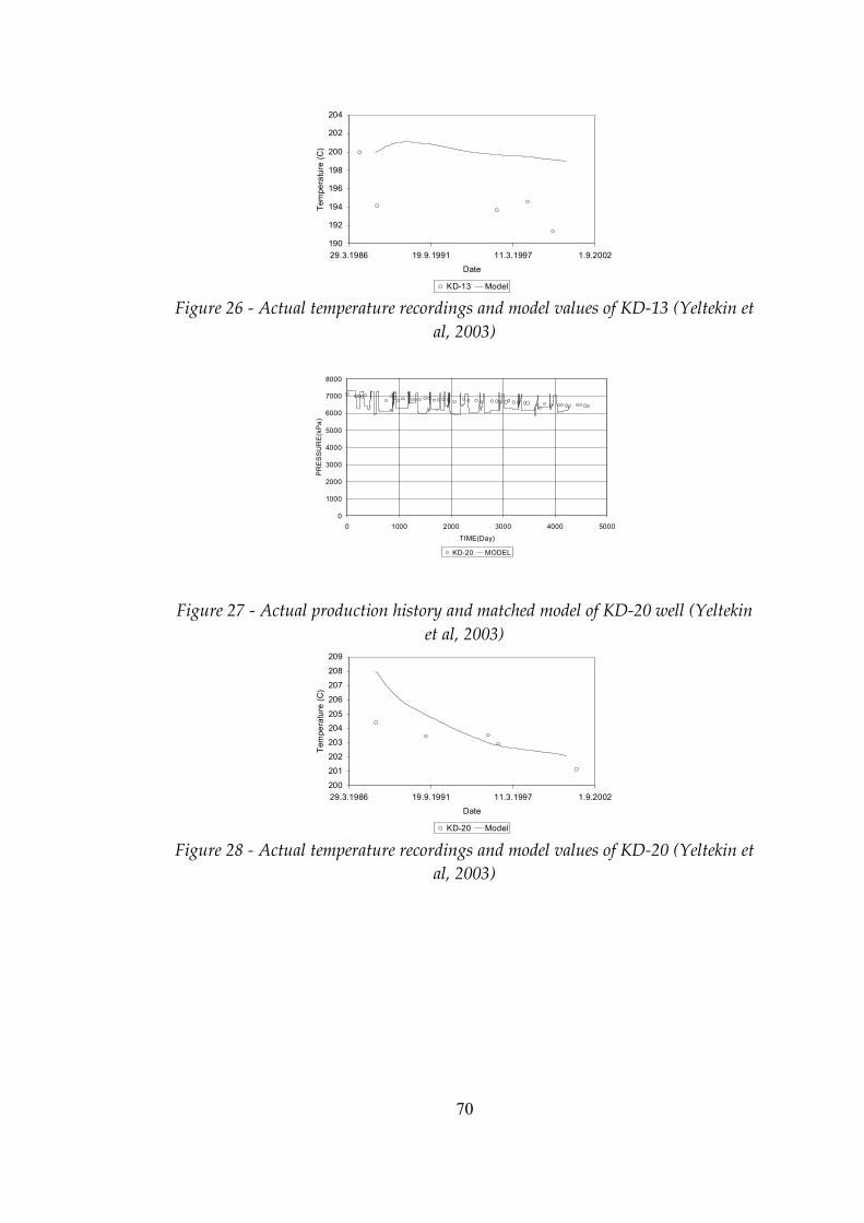
70
190
192
194
196
198
200
202
204
29.3.1986 19.9.1991 11.3.1997 1.9.2002
Date
Temperature (C
)
KD13 Model
Figure 26 ‑ Actual temperature recordings and model values of KD‑13 (Yeltekin et al, 2003)
0
1000
2000
3000
4000
5000
6000
7000
8000
0 1000 2000 3000 4000 5000
TIME(Day)
PRESSURE(kPa)
KD20 MODEL
Figure 27 ‑ Actual production history and matched model of KD‑20 well (Yeltekin et al, 2003)
200
201
202
203
204
205
206
207
208
209
29.3.1986 19.9.1991 11.3.1997 1.9.2002
Date
Temperature (C
)
KD20 Model
Figure 28 ‑ Actual temperature recordings and model values of KD‑20 (Yeltekin et al, 2003)
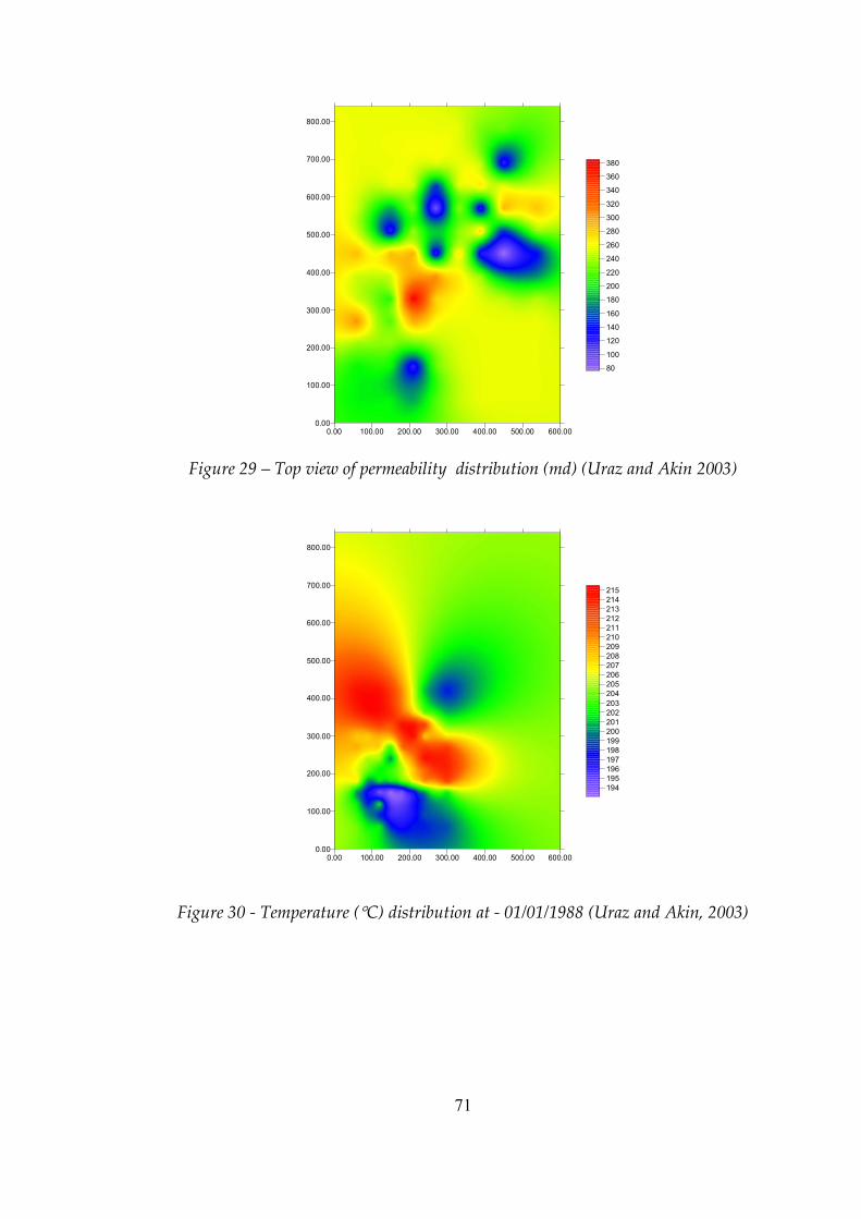
71
0.00 100.00 200.00 300.00 400.00 500.00 600.00 0.00
100.00
200.00
300.00
400.00
500.00
600.00
700.00
800.00
80
100
120
140
160
180
200
220
240
260
280
300
320
340
360
380
Figure 29 – Top view of permeability distribution (md) (Uraz and Akin 2003)
0.00 100.00 200.00 300.00 400.00 500.00 600.00 0.00
100.00
200.00
300.00
400.00
500.00
600.00
700.00
800.00
194 195 196 197 198 199 200 201 202 203 204 205 206 207 208 209 210 211 212 213 214 215
Figure 30 ‑ Temperature (°C) distribution at ‑ 01/01/1988 (Uraz and Akin, 2003)
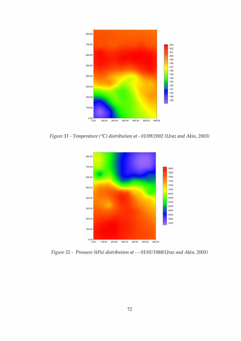
72
0.00 100.00 200.00 300.00 400.00 500.00 600.00 0.00
100.00
200.00
300.00
400.00
500.00
600.00
700.00
800.00
188
189
190
191
192
193
194
195
196
197
198
199
200
201
202
203
Figure 31 ‑ Temperature (°C) distribution at ‑ 01/09/2002 (Uraz and Akin, 2003)
0.00 100.00 200.00 300.00 400.00 500.00 600.00 0.00
100.00
200.00
300.00
400.00
500.00
600.00
700.00
800.00
5400
5600
5800
6000
6200
6400
6600
6800
7000
7200
7400
7600
7800
8000
Figure 32 ‑ Pressure (kPa) distribution at ‑ ‑ 01/01/1988(Uraz and Akin, 2003)
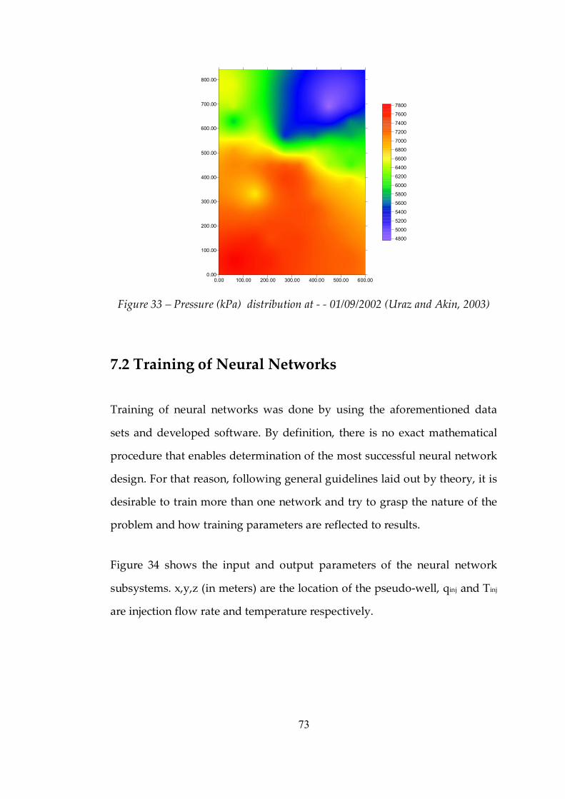
73
0.00 100.00 200.00 300.00 400.00 500.00 600.00 0.00
100.00
200.00
300.00
400.00
500.00
600.00
700.00
800.00
4800
5000
5200
5400
5600
5800
6000
6200
6400
6600
6800
7000
7200
7400
7600
7800
Figure 33 – Pressure (kPa) distribution at ‑ ‑ 01/09/2002 (Uraz and Akin, 2003)
7.2 Training of Neural Networks
Training of neural networks was done by using the aforementioned data
sets and developed software. By definition, there is no exact mathematical
procedure that enables determination of the most successful neural network
design. For that reason, following general guidelines laid out by theory, it is
desirable to train more than one network and try to grasp the nature of the
problem and how training parameters are reflected to results.
Figure 34 shows the input and output parameters of the neural network
subsystems. x,y,z (in meters) are the location of the pseudo‑well, qinj and Tinj
are injection flow rate and temperature respectively.

74
Figure 34 – Input and output parameter configuration of the neural networks
In this study, three different network layouts were used (Table 2).
Table 2 – Summary of Network Layouts
Network 1 Network 2 Network 3 Number of Hidden Layers
1 1 2
Number of Nodes Per Layer
5 20 Layer 1: 10 Layer 2: 5
All of the networks are full connected and have fixed momentum of 0.8. This
fixed value is found appropriate after inspecting various networks with
different parameters. Table 3 shows average training times of all three
networks. The significant difference between single and dual layer networks
is expected. In fully connected networks number of connection increases
non‑linearly when number of layers increase, which is reflected to
calculation time per iteration. Therefore, although Network 3 has less
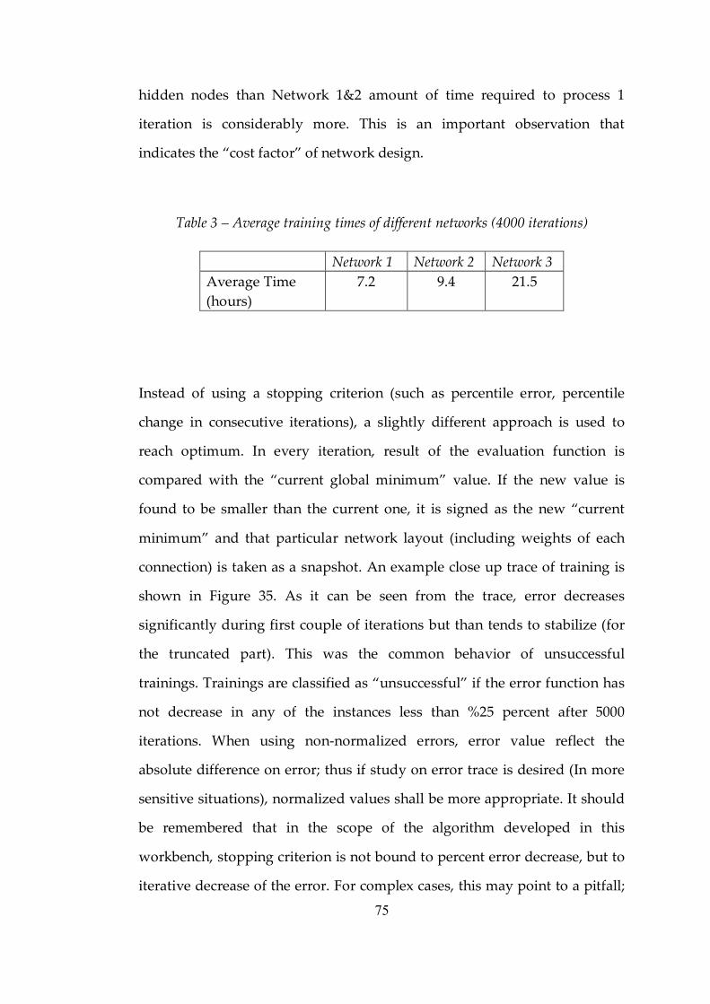
75
hidden nodes than Network 1&2 amount of time required to process 1
iteration is considerably more. This is an important observation that
indicates the “cost factor” of network design.
Table 3 – Average training times of different networks (4000 iterations)
Network 1 Network 2 Network 3 Average Time (hours)
7.2 9.4 21.5
Instead of using a stopping criterion (such as percentile error, percentile
change in consecutive iterations), a slightly different approach is used to
reach optimum. In every iteration, result of the evaluation function is
compared with the “current global minimum” value. If the new value is
found to be smaller than the current one, it is signed as the new “current
minimum” and that particular network layout (including weights of each
connection) is taken as a snapshot. An example close up trace of training is
shown in Figure 35. As it can be seen from the trace, error decreases
significantly during first couple of iterations but than tends to stabilize (for
the truncated part). This was the common behavior of unsuccessful
trainings. Trainings are classified as “unsuccessful” if the error function has
not decrease in any of the instances less than %25 percent after 5000
iterations. When using non‑normalized errors, error value reflect the
absolute difference on error; thus if study on error trace is desired (In more
sensitive situations), normalized values shall be more appropriate. It should
be remembered that in the scope of the algorithm developed in this
workbench, stopping criterion is not bound to percent error decrease, but to
iterative decrease of the error. For complex cases, this may point to a pitfall;
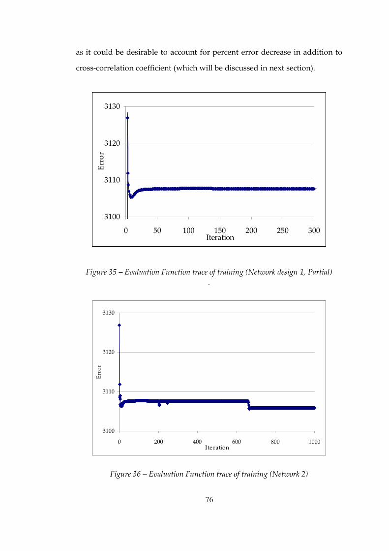
76
as it could be desirable to account for percent error decrease in addition to
cross‑correlation coefficient (which will be discussed in next section).
3100
3110
3120
3130
0 50 100 150 200 250 300 Iteration
Error
Figure 35 – Evaluation Function trace of training (Network design 1, Partial) .
3100
3110
3120
3130
0 200 400 600 800 1000 Iteration
Error
Figure 36 – Evaluation Function trace of training (Network 2)
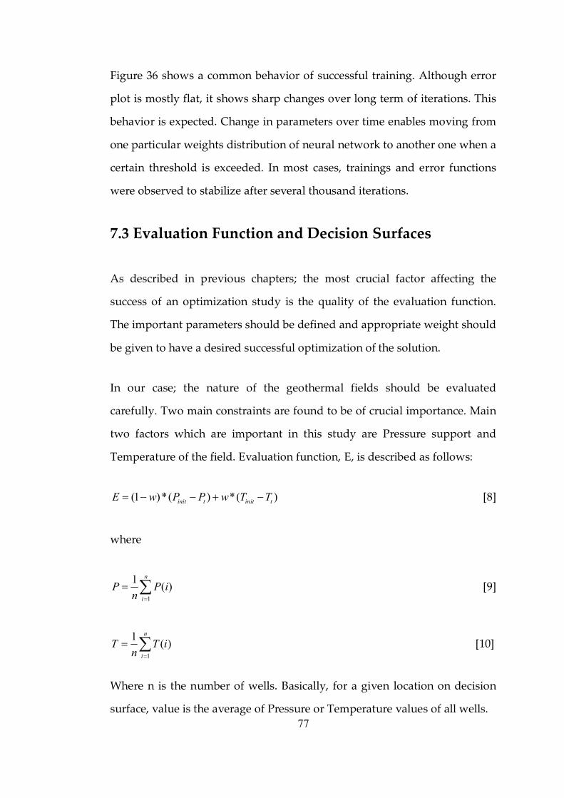
77
Figure 36 shows a common behavior of successful training. Although error
plot is mostly flat, it shows sharp changes over long term of iterations. This
behavior is expected. Change in parameters over time enables moving from
one particular weights distribution of neural network to another one when a
certain threshold is exceeded. In most cases, trainings and error functions
were observed to stabilize after several thousand iterations.
7.3 Evaluation Function and Decision Surfaces
As described in previous chapters; the most crucial factor affecting the
success of an optimization study is the quality of the evaluation function.
The important parameters should be defined and appropriate weight should
be given to have a desired successful optimization of the solution.
In our case; the nature of the geothermal fields should be evaluated
carefully. Two main constraints are found to be of crucial importance. Main
two factors which are important in this study are Pressure support and
Temperature of the field. Evaluation function, E, is described as follows:
(1 )*( ) *( ) init t init t E w P P w T T = − − + − [8]
where
1
1 ( ) n
i
P P i n =
= ∑ [9]
1
1 ( ) n
i
T T i n =
= ∑ [10]
Where n is the number of wells. Basically, for a given location on decision
surface, value is the average of Pressure or Temperature values of all wells.
78
7.3.1 Evaluation Function Properties
Best way to obtain the evaluation function is to ask the question of; “what is
the ultimate goal that is to be improved/optimized”. In our case the answer
is “To locate injection well such that; in the long run, reservoir keeps the
pressure support (so that we can produce more) while injected fluid does
not cool down the field (as maximum enthalpy means more energy).
Designed algorithm handles pressure and temperature separately. Output of
the neural network values are separated in two sets, so that the distribution
of Temperature and Pressure are trained/executed separately. Evaluation
function uses weighted averaging to combine temperature and pressure
values at a given location. This gives a flexibility to put more weight to
different parameters.
Choosing an evaluation function is a process of decision. In our study, it
would be possible to define numerous different evaluation functions;
depending on the optimization target. For instance, it is possible to focus on
Net Present Value (NPV) of the field production (for example as in the case
of Yeten et al, 2003). Our choice for Temperature and Pressure support over
NPV is due to the desire to study change in the basic parameters such as
Temperature and Pressure. As net present value is also a function of
Temperature and Pressure, study carried on the basic parameters and
testing the reliability on those is believed to be more informative in
comparing proposed workflow over numerical methods.
79
7.4 Search Method – Finding Optimum Location
Designed framework enables deployment of various search algorithms such
as exhaustive search, polytope algorithm or simulated annealing. Design
goal is to provide a modular approach to enable problem specific algorithms
to be deployed.
For the case study and to test results of neural network in more detail,
exhaustive search is used. In bigger data sets, exhaustive search would yield
higher CPU cost, there fore more streamlined search algorithms should be
preferred.
Search algorithm uses six parameters:
Discritization interval in X direction (West – East): xd
Discritization interval in Y direction (North – South): yd
Injection temperature of the pseudo‑well: Tinj
Injection flow rate of the pseudo‑well: qinj
Weight of Temperature (in range of 0‑1)
Weight of Pressure (in range of 0‑1 and if no other constraints are
introduced 1 – weight of temperature)
Search algorithm is as follows:
1) Start from North – West corner of the search area. (x0 , y0)
80
2) Place the pseudo well to xi=xo+xd , yi = y0
3) Input neural network the parameter set: qinj , Tinj , xi , yi
4) Record the Pressure and Temperature output of Neural Network nodes
5) Calculate and record the field temperature & pressure response using
equation 9,10 and values of P & T from step 4
6) Calculate the evaluation function result (Equation 8) and record.
7) Proceed to next iteration where: xi+1 = xi+xd , yi = y0
8) Repeat steps 2 ‑ 7 until xi+n >= x (West – East size of the field)
9) Iterate yi= y0 + yd and reset xi = x0
10) Repeat steps 2 – 9 until xi+n+k >= x and yI+k >= y (North – South size of the
field)
Output the minimum E value location (Where E is the evaluation function
result calculated at given location (calculated at Step 6).
Combination of neural network and search algorithms gives a finer
resolution of results than simulation grid size. If xd < Simulation Grid Size ,
discritization in X direction is narrowed allowing a smoother decision
surface than the numerical model (Simulator). It is possible to decrease the
discritization interval as low as desired, although very small intervals will
result with higher CPU cost.

81
In general application, it may not be desirable to record evaluation result of
the whole field. Instead, more cost effective search algorithms that can
march to the result faster should be preferred.
7.6 Comparison of Neural Network results to
Simulation Results
Aforementioned three neural network designs are used to evaluate the
sensitivity of the outputs to layouts. Values obtained from trained networks
are compared to reference simulation results.
For comparison of the results, validation set (described in Chapter 4) is used.
As validation locations are excluded from the training set, they form as a
valid test for neural network performance.
Table 4 and Table 5 shows the Temperature and Pressure values obtained
from Neural Network runs tabulated alongside with reference Simulation
results.
Figure 37 shows the evaluation locations (previously introduced in
Introduced in page 61) that are used for this study.
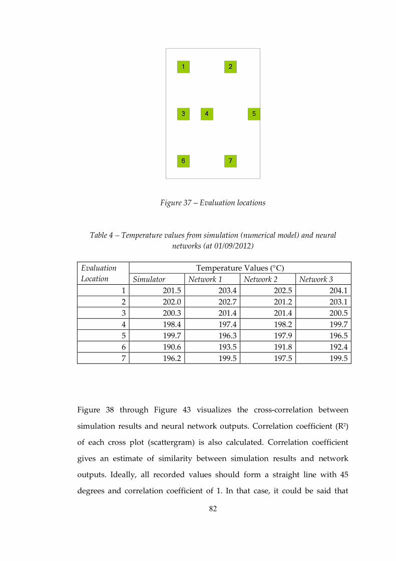
82
Figure 37 – Evaluation locations
Table 4 – Temperature values from simulation (numerical model) and neural networks (at 01/09/2012)
Temperature Values (°C) Evaluation Location Simulator Network 1 Network 2 Network 3
1 201.5 203.4 202.5 204.1 2 202.0 202.7 201.2 203.1 3 200.3 201.4 201.4 200.5 4 198.4 197.4 198.2 199.7 5 199.7 196.3 197.9 196.5 6 190.6 193.5 191.8 192.4 7 196.2 199.5 197.5 199.5
Figure 38 through Figure 43 visualizes the cross‑correlation between
simulation results and neural network outputs. Correlation coefficient (R 2 )
of each cross plot (scattergram) is also calculated. Correlation coefficient
gives an estimate of similarity between simulation results and network
outputs. Ideally, all recorded values should form a straight line with 45
degrees and correlation coefficient of 1. In that case, it could be said that
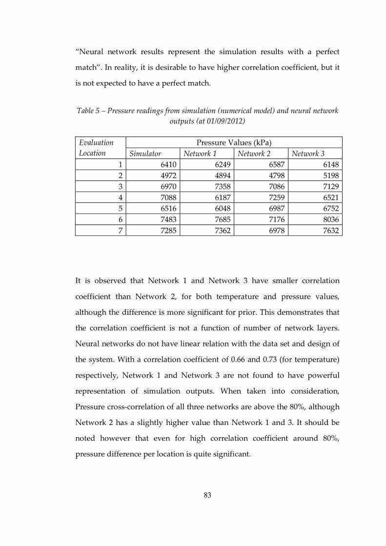
83
“Neural network results represent the simulation results with a perfect
match”. In reality, it is desirable to have higher correlation coefficient, but it
is not expected to have a perfect match.
Table 5 – Pressure readings from simulation (numerical model) and neural network outputs (at 01/09/2012)
Pressure Values (kPa) Evaluation Location Simulator Network 1 Network 2 Network 3
1 6410 6249 6587 6148 2 4972 4894 4798 5198 3 6970 7358 7086 7129 4 7088 6187 7259 6521 5 6516 6048 6987 6752 6 7483 7685 7176 8036 7 7285 7362 6978 7632
It is observed that Network 1 and Network 3 have smaller correlation
coefficient than Network 2, for both temperature and pressure values,
although the difference is more significant for prior. This demonstrates that
the correlation coefficient is not a function of number of network layers.
Neural networks do not have linear relation with the data set and design of
the system. With a correlation coefficient of 0.66 and 0.73 (for temperature)
respectively, Network 1 and Network 3 are not found to have powerful
representation of simulation outputs. When taken into consideration,
Pressure cross‑correlation of all three networks are above the 80%, although
Network 2 has a slightly higher value than Network 1 and 3. It should be
noted however that even for high correlation coefficient around 80%,
pressure difference per location is quite significant.

84
It is observed that Network 2 has the highest correlation coefficient for both
parameters, 0.9076 for temperature and 0.887 for pressure with accurate
representation of reference simulation results. Following this analysis
indicates that Network 2 is preferred for further calculations and location
estimation, as it acts as a better proxy to simulator. It was also observed that
the large errors recorded in the positions that reside in the middle of the
field are somehow consistent through networks. This is accounted for the
lack of capability in capturing transient effects that are dominant in middle
region of the field due to large number of producing wells.
Ideally, this selection process can be automated; picking the network with
highest correlation at a given time. If processing time and power is not a
constraint, it is possible to expand the number of networks trained thus
exploring a wider space of cross correlation. It should be noted that, time
requirement of the framework increases non‑linearly with introduction of
more neural networks. Nevertheless, framework provides flexibility on
number of trials (new network designs to be trained).
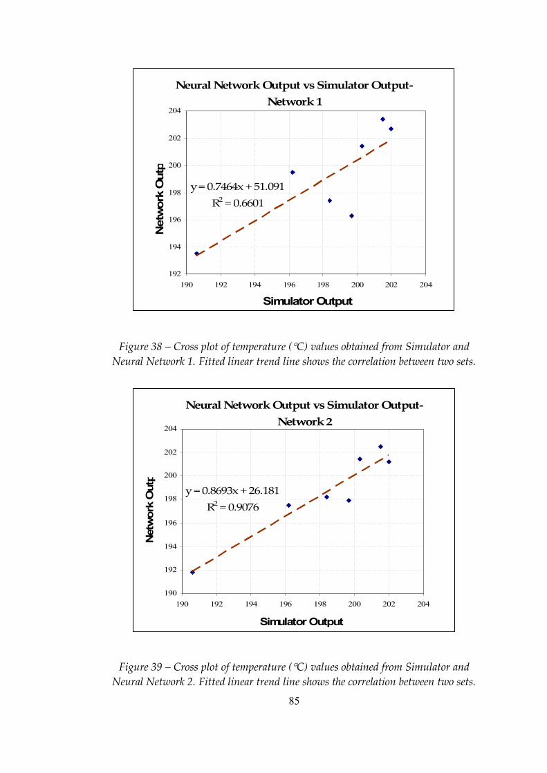
85
Neural Network Output vs Simulator Output‑ Network 1
y = 0.7464x + 51.091 R 2 = 0.6601
192
194
196
198
200
202
204
190 192 194 196 198 200 202 204
Simulator Output
Network Output
Figure 38 – Cross plot of temperature (°C) values obtained from Simulator and Neural Network 1. Fitted linear trend line shows the correlation between two sets.
Neural Network Output vs Simulator Output‑ Network 2
y = 0.8693x + 26.181 R 2 = 0.9076
190
192
194
196
198
200
202
204
190 192 194 196 198 200 202 204
Simulator Output
Network Output
Figure 39 – Cross plot of temperature (°C) values obtained from Simulator and Neural Network 2. Fitted linear trend line shows the correlation between two sets.
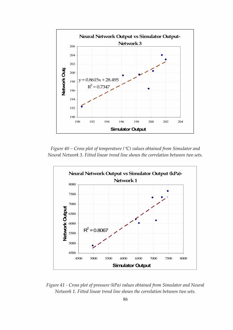
86
Neural Network Output vs Simulator Output‑ Network 3
y = 0.8615x + 28.495 R 2 = 0.7347
190
192
194
196
198
200
202
204
206
190 192 194 196 198 200 202 204
Simulator Output
Network Output
Figure 40 – Cross plot of temperature (°C) values obtained from Simulator and Neural Network 3. Fitted linear trend line shows the correlation between two sets.
Neural Network Output vs Simulator Output (kPa)‑ Network 1
R 2 = 0.8067
4500
5000
5500
6000
6500
7000
7500
8000
4500 5000 5500 6000 6500 7000 7500 8000
Simulator Output
Network Output .
Figure 41 ‑ Cross plot of pressure (kPa) values obtained from Simulator and Neural Network 1. Fitted linear trend line shows the correlation between two sets.
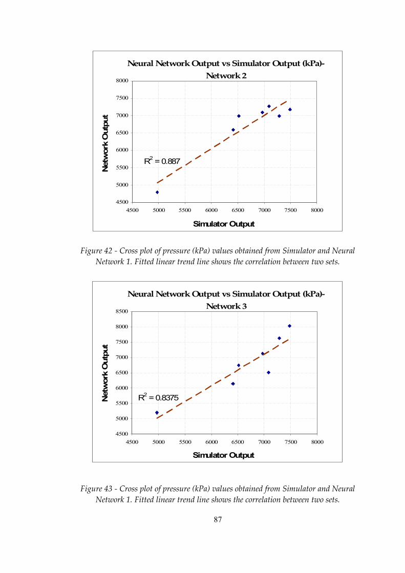
87
Neural Network Output vs Simulator Output (kPa)‑ Network 2
R 2 = 0.887
4500
5000
5500
6000
6500
7000
7500
8000
4500 5000 5500 6000 6500 7000 7500 8000
Simulator Output
Network Output .
Figure 42 ‑ Cross plot of pressure (kPa) values obtained from Simulator and Neural Network 1. Fitted linear trend line shows the correlation between two sets.
Neural Network Output vs Simulator Output (kPa)‑ Network 3
R 2 = 0.8375
4500
5000
5500
6000
6500
7000
7500
8000
8500
4500 5000 5500 6000 6500 7000 7500 8000
Simulator Output
Network Output .
Figure 43 ‑ Cross plot of pressure (kPa) values obtained from Simulator and Neural Network 1. Fitted linear trend line shows the correlation between two sets.
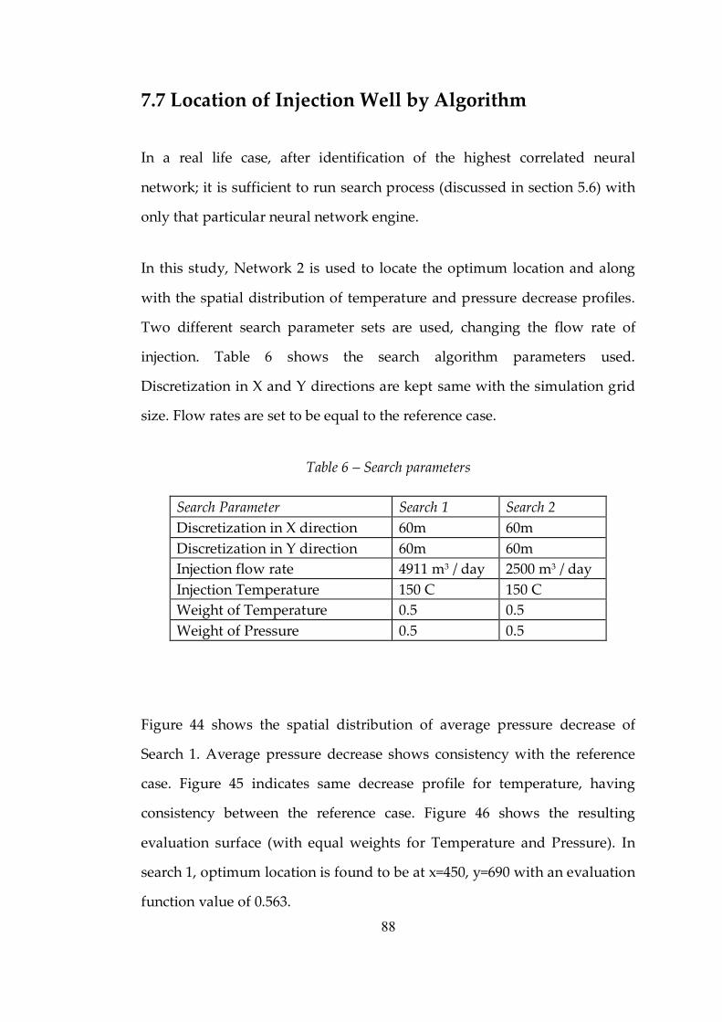
88
7.7 Location of Injection Well by Algorithm
In a real life case, after identification of the highest correlated neural
network; it is sufficient to run search process (discussed in section 5.6) with
only that particular neural network engine.
In this study, Network 2 is used to locate the optimum location and along
with the spatial distribution of temperature and pressure decrease profiles.
Two different search parameter sets are used, changing the flow rate of
injection. Table 6 shows the search algorithm parameters used.
Discretization in X and Y directions are kept same with the simulation grid
size. Flow rates are set to be equal to the reference case.
Table 6 – Search parameters
Search Parameter Search 1 Search 2 Discretization in X direction 60m 60m Discretization in Y direction 60m 60m Injection flow rate 4911 m 3 / day 2500 m 3 / day Injection Temperature 150 C 150 C Weight of Temperature 0.5 0.5 Weight of Pressure 0.5 0.5
Figure 44 shows the spatial distribution of average pressure decrease of
Search 1. Average pressure decrease shows consistency with the reference
case. Figure 45 indicates same decrease profile for temperature, having
consistency between the reference case. Figure 46 shows the resulting
evaluation surface (with equal weights for Temperature and Pressure). In
search 1, optimum location is found to be at x=450, y=690 with an evaluation
function value of 0.563.

89
2 4 6 8
2
4
6
8
10
12 0.7
0.71
0.72
0.73
0.74
0.75
0.76
0.77
0.78
0.79
0.8
Figure 44 – Spatial distribution of average pressure decrease (Search 1).
2 4 6 8
2
4
6
8
10
12
0.2
0.22
0.24
0.26
0.28
0.3
0.32
Figure 45 ‑ Spatial distribution of average temperature decrease (Search 1)
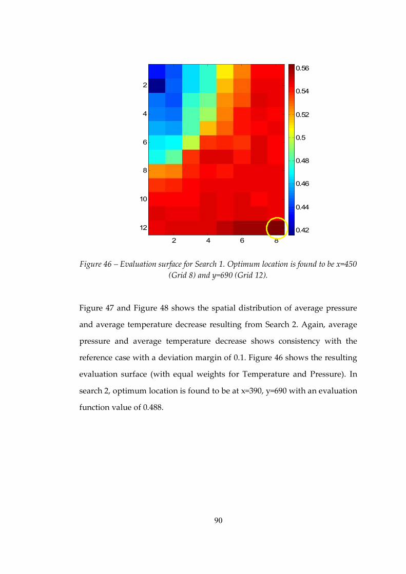
90
2 4 6 8
2
4
6
8
10
12 0.42
0.44
0.46
0.48
0.5
0.52
0.54
0.56
Figure 46 – Evaluation surface for Search 1. Optimum location is found to be x=450 (Grid 8) and y=690 (Grid 12).
Figure 47 and Figure 48 shows the spatial distribution of average pressure
and average temperature decrease resulting from Search 2. Again, average
pressure and average temperature decrease shows consistency with the
reference case with a deviation margin of 0.1. Figure 46 shows the resulting
evaluation surface (with equal weights for Temperature and Pressure). In
search 2, optimum location is found to be at x=390, y=690 with an evaluation
function value of 0.488.

91
2 4 6 8
2
4
6
8
10
12 0.3
0.31
0.32
0.33
0.34
0.35
0.36
0.37
0.38
0.39
0.4
Figure 47 ‑ Spatial distribution of average pressure decrease (Search 2).
2 4 6 8
2
4
6
8
10
12 0.44
0.46
0.48
0.5
0.52
0.54
0.56
Figure 48 ‑ Spatial distribution of average temperature decrease (Search 2)
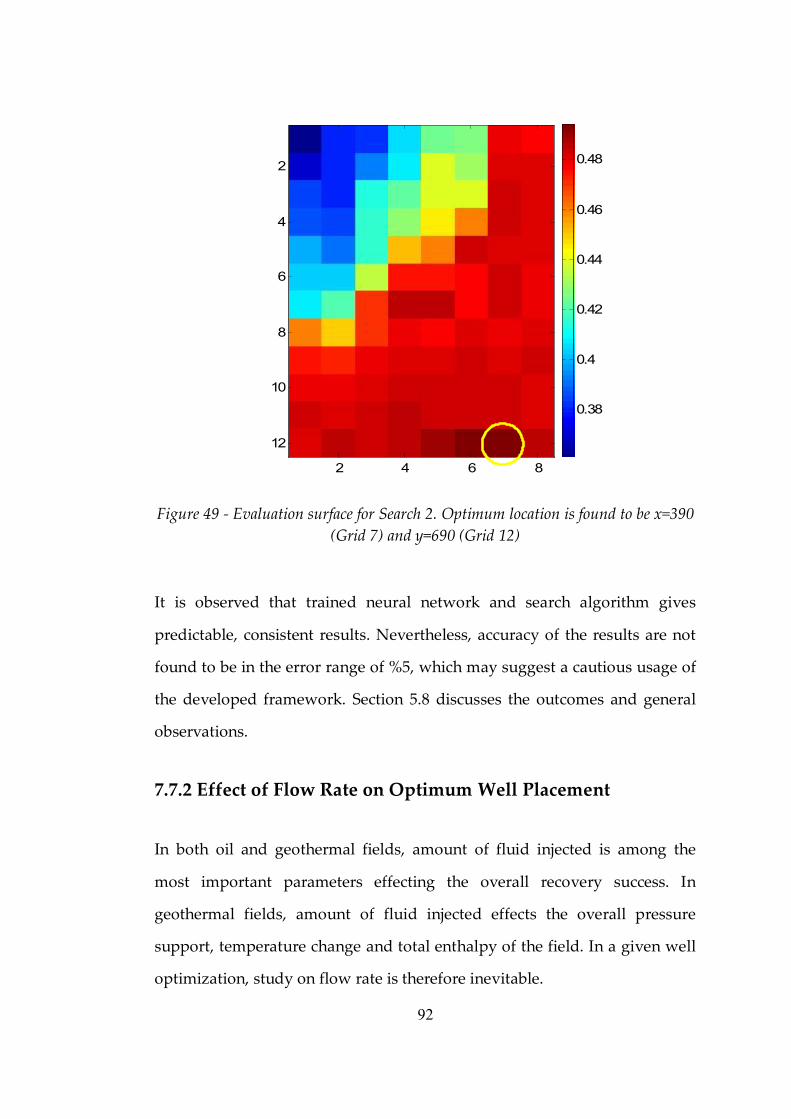
92
2 4 6 8
2
4
6
8
10
12
0.38
0.4
0.42
0.44
0.46
0.48
Figure 49 ‑ Evaluation surface for Search 2. Optimum location is found to be x=390 (Grid 7) and y=690 (Grid 12)
It is observed that trained neural network and search algorithm gives
predictable, consistent results. Nevertheless, accuracy of the results are not
found to be in the error range of %5, which may suggest a cautious usage of
the developed framework. Section 5.8 discusses the outcomes and general
observations.
7.7.2 Effect of Flow Rate on Optimum Well Placement
In both oil and geothermal fields, amount of fluid injected is among the
most important parameters effecting the overall recovery success. In
geothermal fields, amount of fluid injected effects the overall pressure
support, temperature change and total enthalpy of the field. In a given well
optimization, study on flow rate is therefore inevitable.
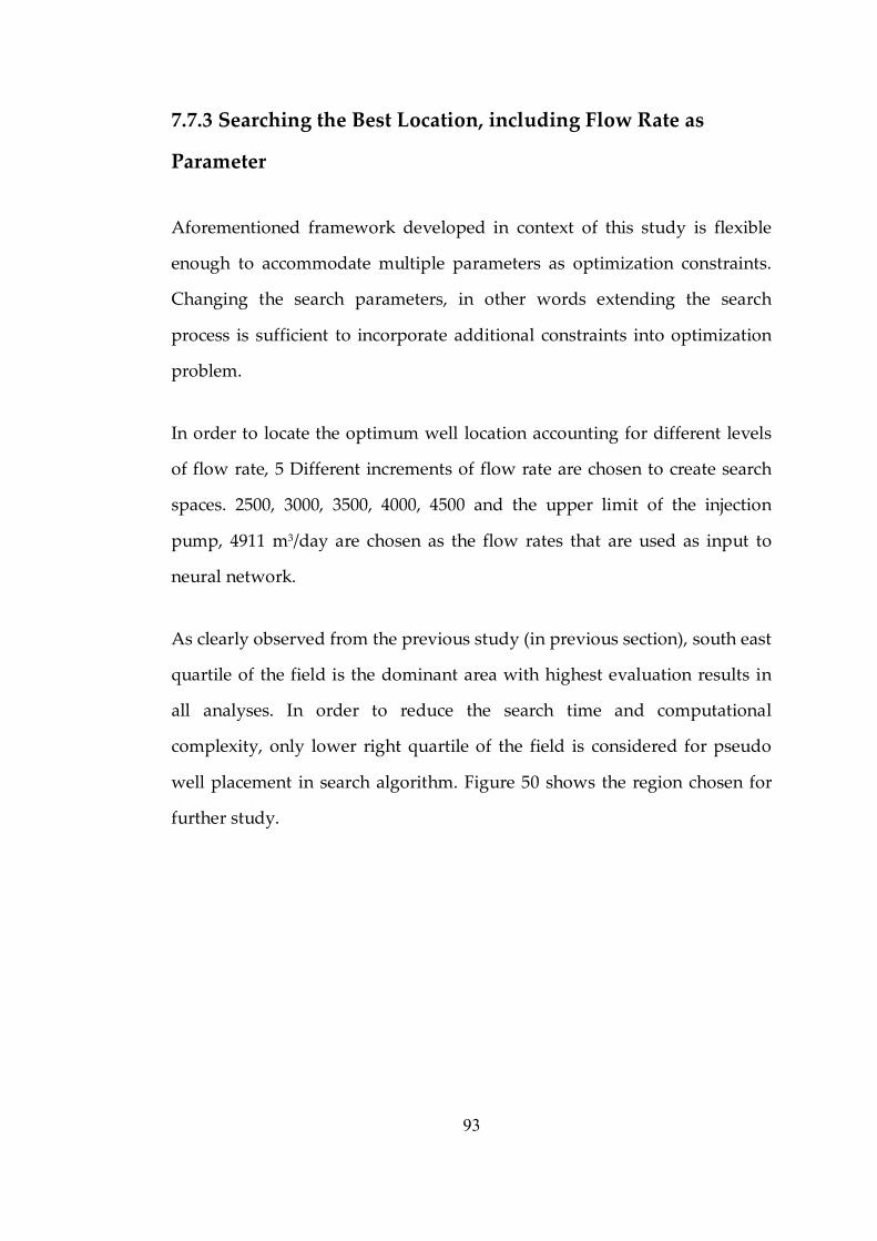
93
7.7.3 Searching the Best Location, including Flow Rate as
Parameter
Aforementioned framework developed in context of this study is flexible
enough to accommodate multiple parameters as optimization constraints.
Changing the search parameters, in other words extending the search
process is sufficient to incorporate additional constraints into optimization
problem.
In order to locate the optimum well location accounting for different levels
of flow rate, 5 Different increments of flow rate are chosen to create search
spaces. 2500, 3000, 3500, 4000, 4500 and the upper limit of the injection
pump, 4911 m 3 /day are chosen as the flow rates that are used as input to
neural network.
As clearly observed from the previous study (in previous section), south east
quartile of the field is the dominant area with highest evaluation results in
all analyses. In order to reduce the search time and computational
complexity, only lower right quartile of the field is considered for pseudo
well placement in search algorithm. Figure 50 shows the region chosen for
further study.
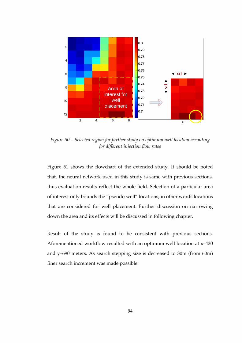
94
2 4 6 8
2
4
6
8
10
12 0.7
0.71
0.72
0.73
0.74
0.75
0.76
0.77
0.78
0.79
0.8
6 8
Figure 50 – Selected region for further study on optimum well location accouting for different injection flow rates
Figure 51 shows the flowchart of the extended study. It should be noted
that, the neural network used in this study is same with previous sections,
thus evaluation results reflect the whole field. Selection of a particular area
of interest only bounds the “pseudo well” locations; in other words locations
that are considered for well placement. Further discussion on narrowing
down the area and its effects will be discussed in following chapter.
Result of the study is found to be consistent with previous sections.
Aforementioned workflow resulted with an optimum well location at x=420
and y=690 meters. As search stepping size is decreased to 30m (from 60m)
finer search increment was made possible.
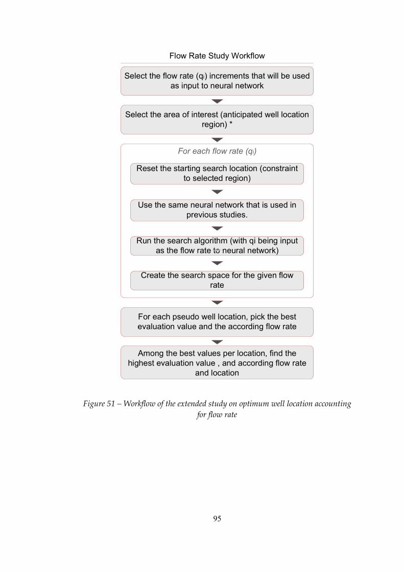
95
Select the area of interest (anticipated well location region) *
For each flow rate (qi)
Reset the starting search location (constraint to selected region)
Run the search algorithm (with qi being input as the flow rate to neural network)
Among the best values per location, find the highest evaluation value , and according flow rate
and location
Flow Rate Study Workflow
Select the flow rate (qi) increments that will be used as input to neural network
Use the same neural network that is used in previous studies.
Create the search space for the given flow rate
For each pseudo well location, pick the best evaluation value and the according flow rate
Figure 51 – Workflow of the extended study on optimum well location accounting for flow rate

96
Flow Rate vs. Evaluation
0 0.1 0.2 0.3 0.4 0.5
0.6
2000 3000 4000 5000 Flow Rate (m3 / day)
Evaluation Fu
nctio
n .
Eval Func Val
Reversed Eval Func
Figure 52 – Evaluation function values at the optimum location with respect to different flow rates
Figure 52 shows the evaluation function results in this particular location
with respect to different injection flow rates. It is observed that, highest
evaluation value was recorded with an injection flow rate of 4000 m 3 / day.
The fact that equal weights are used for temperature and pressure seems to
be the source of a balanced flow rate being favorable.
7.8 Comparison with Previous Studies
Results obtained from this study is compared to previous studies on
Kizildere geothermal field.
Yeltekin et al (2003) studied 5 different injection scenarios on the same field
for same time period (ending in 2012). In first two cases, KD‑7 was used as
reinjection well with constant injection rate of 2500 m 3 /day or 900o kPa fixed
bottom hole pressure. For the third and forth cases, KD‑22 was used with
constant injection rate of 4500 m 3 /day or 9000 kPa fixed bottom hole

97
pressure. Last two cases used KD‑24 as injection location again with 4500
m 3 /day or 9000 kPa.
Using KD‑22 as reinjection location (located in middle of the field) did not
increase production considerably but resulted with maximum pressure
support. In comparison with our methodology, re‑inection to central part of
the field seemed to be in contradiction to some extend, though can be
argued due to the lack of exact locations for comparison. Nevertheless, by
the help of introduced framework, as more possibilities were tested, location
of well was spotted in south‑east region is an option that has not been
investigated in the study. Serpen and Satman , in their study suggested
injection from northern part of the region, where permeability is higher,
thus yielding to higher sweep ratio of the region.
7.9 Summary of Results
Following are the final remarks on the results obtained from the study.
Design parameters of the network do not provide a measure of success of
estimation. Study on different networks indicates that there is no direct
relation between the design parameters and the output of the network.
Having different number of nodes and layers, all three networks resulted
with different correlation coefficients ranging from 0.60 to 0.90 with no
particular relation to design parameters.
As different network designs can yield to considerably different correlation
coefficients between simulation and neural network values for a successful
prediction of simulation results, a neural network design with at least %90
98
cross correlation should be used. If possible, study of different layouts
should be extended to improve the correlation.
Study on correlation coefficients for pressure and temperature indicate that
for the case study, Temperature correlation coefficients vary more than the
pressure correlation coefficients. This indicates the necessity of special
attention that should be paid for choosing the governing parameters for
network selection.
For the field of study (Kızıldere Geothermal field), optimum injection well
location is found to be in the south‑eastern part of the field. Having higher
evaluation function values in that particular region, specific locations
resulting from the workflow indicated a consistent search space.
When studied with fixed flow rates (2500 and 4911 m 3 /day), search run
through the whole field located two locations which are in the same region;
thus resulting with consistent predictions.
Study accounting for flow rate indicated that injection flow rate is an
important factor and should be considered in such optimization problem.
When included in the input parameter set and search constraints, it was
observed that having different flow rates altered the optimum location;
though remaining consistent with previous calculations.

99
CHAPTER 8
CONCLUSION
Results indicate that usage of neural networks provide a convenient way of
reducing processing demand. Especially in large fields, cost of doing an
exhaustive search is beyond feasible limits and proposed framework could
be deployed in such cases. Although results obtained from the case study
indicate a favorable and acceptable correlation between simulation results
and neural network results; it is found that neural networks shall not be
used as a replacement for simulators due to high error margins and design
issues. Study indicated following observations:
Introduction of neural networks provide a convenient way of reducing
simulations costs. Inference capability of ANN is suitable to replicate the
response of earth given a set of limited parameters.
Design of the Neural Network is an important factor determining the
success of the decision. Through study of cross correlation between
simulation and neural network results, it was observed that different
network layouts result with considerably different correlation factors.
It is suggested that, although proposed framework can produce acceptable
results (given a well trained network) for narrowing down the search area or
incorporating various parameters without increasing data redundancy, it
shall not be used as a replacement for numerical simulator. This conclusion
is drawn from the fact that correlation of the results are more than the
acceptable %5 limit and vary considerably depending on the network. The
cost effective nature of the framework provides a convenient way of
100
exploring wider space of parameters, eliminating need for exhaustive
simulation runs but results are not accepted to be accurate enough to replace
numerical/analytical models.
It should be noted that the “optimum well locations” picked by the
framework incorporate a specific set of parameters on evaluation function;
for real life deployment it is suggested to use different evaluation functions
or a combination of additional constraints for future refinement of location
selection. Location of the well is a function of Evaluation function.
Flexibility of the framework enabled extending the study by considering
only a particular area of interest (see study on flow rate). After training a
neural network that incorporates the whole field, narrowing down the
search area or the area of consideration for well placement can be achieved
by only narrowing the search area. This feature is also found intuitively
parallel to real life cases, as it is a common practice to narrow down the area
of interest after certain studies; when it is concluded that there exists a
particular area of the field that the most feasible location lies.
A further study could incorporate more parameters as variable; such as dept
of injection, different temperatures of injection and changing injection rates
over time.

101
REFERENCES
Aanonsen, S. I., Eide, A. L., Holden, L., and Aasen, J. O. (1995). Optimizing
Reservoir Performance Under Uncertainty with Application toWell Location, paper
SPE 30710 presented at the SPE Annual Technical Conference & Exhibition,
Dallas, Texas, October 22‑25.
Akın, S., Yeltekin K. and Parlaktuna M. (2003). “Numerical Modeling of
Kızıldere Geothermal Field, Turkey” European Geothermal Conference ‑ 25‑30,
Szeged, Hungary.
Al‑Hanai, W., Russell, S. D., Vissapragada, B. (2000). An Article on Carbonate
Rocks, compiled by Al‑Hanai et al.
Ali, J. K. (1994). Neural Networks: A New Tool for the Petroleum Industry. Paper
SPE 27561 presented at the 1994 European Petroleum Computer Conference,
Aberdeen, U.K., March 15‑17.
Aminian, K., Bilgesu, H.I., Ameri, S. (2000). Improving the simulation of
waterflood performance with the use of neural networks, paper SPE 65630
presented at the 2000 SPE Regional Meeting, West Virginia, 17‑19 October.
Anderson, J. A. (1995). An Introduction to Neural Networks. MIT Press,
Cambridge, MA.
Arkan, S., Akin, S., Parlaktuna, M. (2002). Effect of Calcite Scaling on
PressureTransient Analysis of Geothermal Wells, Proceedings of Twenthy‑
Seventh Workshop on Geothermal Reservoir Engineering, Stanford,
California, January 28‑30.

102
Axelsson, G., Dong, Z. (1998). The Tanggu Geothermal Reservoir (Tianjin,
China). Geothermics, 27 (3), 271‑294.
Beckner, B. L. and Song, X. (1995). Field Development Planning Using
Simulated Annealing ‑ Optimal Economic Well Scheduling and Placement, paper
SPE 30650 presented at the SPE Annual Technical Conference & Exhibition,
Dallas, Texas, October 22‑25.
Bodvarsson, G. (1970). Report on an Investigation Concerning the Subsurface
Disposal of Effluent Thermal Waters from a 30MW Geothermal Power Plant at
Ahuachapan. UN Development Program Survey of Geothermal Resources, El
Salvador, Project Report.
Bodvarsson, G., Pruess, K., OʹSullivan, M. J. (1985). Injection and energy
recovery in fractured geothermal reservoirs. Paper, SPE 15344, Society of
Petroleum Engineers Journal, volume 25, pp 303‑312.
Bodvarsson, G., Stefansson, V. (1988). Reinjection into Geothermal Reservoirs.
Geothermal Reservoir Engineering, Edited Okandan, E, pp 103‑120, Kluwer
Academic, Dordrecht.
Calore, C., Pruess, K., Celati, R. (1986). Modeling Studies of Cold Water
Injection into Fluid‑Depleted Vapor‑Dominated Geothermal reservoirs.
Proceedings 11 th Workshop on Geothermal Reservoir Engineering, Stanford
University, California, USA, pp 161‑168.
Caers, J. (2004). Lecture notes on Optimization, Stanford University, USA.
Centilmen, A., Ertekin, T., and Grader, A. S. (1999). Applications of Neural
Networks in Multiwell Field Development, paper SPE 56433 presented at the

103
SPE Annual Technical Conference & Exhibition, Houston, Texas, October 3‑
6.
CMG, (2002). Computer Modelling Group Ltd. Alberta, Canada
(www.cmgroup.com)
DeGroot, M. (1970). Optimal Statistical Decisions. McGraw‑Hill, New York,
USA.
Dominco, E., (1974) “Geothermal Energy Survey of Western Anatolia‑Project
Findings and Recommendations”, Report to United Nations Development
Programme.
Doraisamy, H., Ertekin, T., Grader, A.S. (1998). Key Parameters Controlling the
Performance of Neuro‑Simulation Development, paper SPE 51079.
Einarsson, S.S., Vides, A., Cuellar, G. (1975). Disposal of Geothermal Waste
Water by Reinjection, 2 nd United Nations Symposium on Development of
Geothermal Resources, 2, pp 1349‑1363.
Erdogan, M., Mudford, B., Chenoweth, G., Holeywell, R., and Jakubson, J.
(2001). Optimization of Decision Tree and Simulation Portfolios: A Comparison,
paper SPE 68575 presented at the SPE Hydrocarbon Economics and
Evaluation Symbosium, Dallas, Texas, April 2‑3.
Farshad, F., Garber, J.D., Lorde, J.N. (1999). Predicting Temperature Profiles in
Producing Oil Wells Using Artificial Neural Networks, paper SPE 53738.
Gill, P. E., Murray, W., and Wright, M. H. (1981). Practical Optimization.
Academic Press, London, UK.
104
Goyal, K. P., (1999). Injection Related Cooling in the Unit 13 Area of the
Southeast Geysers, California, USA. Geothermics, 28, pp 3‑19.
Guyaguler, B. and Gumrah, F. (1999). Comparison of Genetic Algorithm with
Linear Programming for the Optimization of an Underground Storage Field. IN
SITU, 23(2), pp 131–150.
Guyaguler, B., Horne, R. N., Rogers, L., and Rosenzweig, J. J. (2000).
Optimization of Well Placement in a Gulf of Mexico Waterflooding Project, paper
SPE 63221 presented at the SPE Annual Technical Conference and
Exhibition, Dallas, Texas, October 1‑4. to appear in SPEREE 2002.
Guyaguler, (2003), Optimization of Well Placement and Assessment of
Uncertainty, PhD Thesis, Stanford University, California, USA.
Holland, J. H. (1975). Adaptation in Natural and Artificial Systems. The
University of Michigan Press, Ann Harbor.
James, R., (1979). Reinjection Strategy. Proceedings 5 th Workshop on
Geothermal Reservoir Engineering, Stanford University, Stanford,
California, USA, pp 355‑359.
Kappa, (2001). Kappa Software package by Kappa Engineering
(www.kappaeng.com)
Kumoluyi, A,O., Daltaban, T.S. (1994). Higher‑Order Neural Networks in
Petroleum Engineering, paper SPE 27905 presented at the Western Regional
Meeting in Long Beach, California, U.S.A. 23‑25 March 1994.
105
Lippman, M. J., Tsang, C.F., Witherspoon, P.A., (1977). Analysis of the
response of geothermal reservoirs under injection and production procedures. Paper
SPE 6537, presented at the 47 th Annual California Regional Meeting of
SPE_AIME, Bakersfield, California.
Mitchell, T. (1999),Machine Learning, McGraw Hill Press, New Jersey.
Milora, S., and Tester, J. W. (1976). Geothermal Energy as a Source of Electric
Power. Cambridge, Mass., MIT Press, 1976.
Nelder, J. and Mead, R. (1965). A Simplex Method for Function
Minimization.Computer Journal, 7, pp 308–313.
Okandan, E. (1988). Geothermal Reservoir Engineering, NATO ASI Series,
Series E: Applied Sciences – Vol 150, 1988, Kluwer Academic Publishers
Dordrecht.
Okandan, E. (1988). Importance of Geothermal Reservoir Engineering in the
Assesment of Geothermal Sources, Middle East Technical University, Turkey.
Published in book Geothermal Reservoir Engineering (Okandan, 1988), pp
1‑6.
Pan, Y. and Horne, R. N. (1998). Improved Methods for Multivariate
Optimization of Field Development Scheduling and Well Placement Design, paper
SPE 49055 presented at the SPE Annual Technical Conference & Exhibition,
New Orleans, Texas, September 27‑30. (Also JPT, December 1998).
Rahman, M., Sunbul, M.B., McGuire, M. D. (1991). Case Study: Performance of
a Complex Carbonate Reservoir Under Peripheral Water Injection. Paper SPE
106
21370 presentat at the SPE Middle East Oil Show at Bahrain, 18‑19
November, 1991.
Rian, D. T. and Hage, A. (1994). Automatic Optimization of Well Locations in a
North Sea Fractured Chalk Reservoir Using a Front Tracking Reservoir Simulator,
SPE 28716 presented at the SPE International Petroleum & Exhibition of
Mexico, Veracruz, Mexico, October 10‑13, 1994.
Rogers, L. L. and Dowla, F. U. (1994). “Optimal Groundwater Remediation
Using Artificial Neural Networks with Parallel Solute Transport”. Water
Resources Research, 30(2), pp 457–481.
Russell, S. J. and Norvig, P. (1995). Artificial Intelligence, A Modern Approach.
Prentice Hall, New Jersey.
Serpen, Ü., Satman, A., (2000). Reassessment of the Kızıldere Geothermal
Reservoir, Proceedings World Geothermal Congress 2000, Kyushu‑Tohuku,
Japan, May 28‑June 10, 2869‑2874.
Serpen, Ü., Onur, M., (2001). Analysis of Pressure Transient Tests in Kizildere
Geothermal Field. Proceedings of Twenty‑Sixth Workshop on Geothermal
Reservoir Engineering, Stanford University, Stanford, California, January
29‑31.
Serpen, Ü. (2002). Reinjection Strategy for Kızıldere Geothermal Field.
Proceedings of Twenty‑Seventh Workshop on Geothermal Reservoir
Engineering, Stanford University, Stanford, California, January 28‑30.
Stefansson, V., (1997). Geothermal Reinjection Experience. Geothermics, 26 (1),
pp 99‑139.
107
Stoisits, R. F., Crawford, K. D., MacAllister, D. J., Lawal, A. S., and Ogbe, D.
O. (1999). Production Optimization at the Kuparuk River Field Utilizing Neural
Networks and Genetic Algorithms, paper SPE 52177 presented at the Mid‑
Continent Operations Symposium, Oklahoma City, Oklahoma, March 28‑31.
Suryanarayana, K., Lahiri, G. Characterization of a Complex Carbonate
Reservoir: A Case Study from a Western Offshore Field of India. Paper, SPE 36193
presented at the 7 th Abu Dhabi International Petroleum Exhibition and
Conference, Abu Dhabi, U.A.E., 13‑16 October, 1996.
Şimşek, Ş., (1985) “Geothermal Model of Denizli, Sarayköy‑Buldan Area”
Geothermics, 14 , No.2/3 , 393‑417
Yeltekin K., Parlaktuna M., and Akın, S. (2002). Modeling of Kızıldere
Geothermal Reservoir, Turkey. Proceedings of the Twenty‑Seventh Workshop
on Geothermal Reservoir Engineering Stanford University, Stanford,
California, U.S.A.
Yeten, B., Durlofsky, L.J., Aziz, K. (2003). Optimization of nonconventional well
type, location, and trajectory. SPE Journal, 8, 200‑210 (also paper SPE 77565)
Uraz, I., Akin, S. (2003). “Optimization of Reinjection in Geothermal Reservoirs”,
Proceedings of the Twenty‑Eighth Workshop on Geothermal Reservoir
Engineering, Stanford University, Stanford, California, USA

108
APPENDIX A
SOFTWARE
Software Installation
Provided with this document, a CD including the source code and
executable of the Artificial Intelligence workbench is provided. To install the
executable version of the software:
1) Install Java Runtime Enviroment – Provided in the CD, you will find Sun
Microsystems Java Runtime Enviroment that is required by the AI
Workbench software. It can be installed by executing the Jre.exe file in
the home directory. (If Java Runtime Enviroment 1.4 or higher is already
installed, this step is not necessary).
2) Install Artificial Intelligence Workbench – To install the software, run the
AIWorkbench.exe file and follow the installation instructions when
prompted.
Source code can be accesed by unzipping the provided archive file in the
CD.
109
APPENDIX – B
KIZILDERE GEOTHERMAL FIELD
Located in the western Turkey, Kızıldere geothermal field was discovered in
1968 (Figure 53). The Menderes massif (where Kızıldere is locaed on the
western extreme) was uplifted during late Pliocene and Quaternary times,
and due to tensional forces, east‑est grabens are formed. Magma activity
increased and magma level raised under the massif and grabens where earth
crust is thinner then the rest of the region. The field lies on three main fault
blocks, generated by two‑step normal faults.
Kızıldere geothermal field consists of two producing reservoirs in the
intermediate block. İğdecik formation, the main reservoir formation, is sited
in the metamorphic basement and has very high fracture permeability due
to its crystalline limestone content. Sazak formation, which locally forms the
caprock lies above İğdecik, Kızılburun, Kolonkaya formations. Maximum
temperatures of Sazak and İğdecik formations are 198 °C and 209.1 °C,
respectively (Yeltekin et al, 2002).
Well configuration of Kızıldere Geothermal Field
With the discovery of the field in 1968, the first well; at a depth of 540m was
drilled in the same year and produced a mixture of water and steaam with a
reservoir temperature of 198 °C.
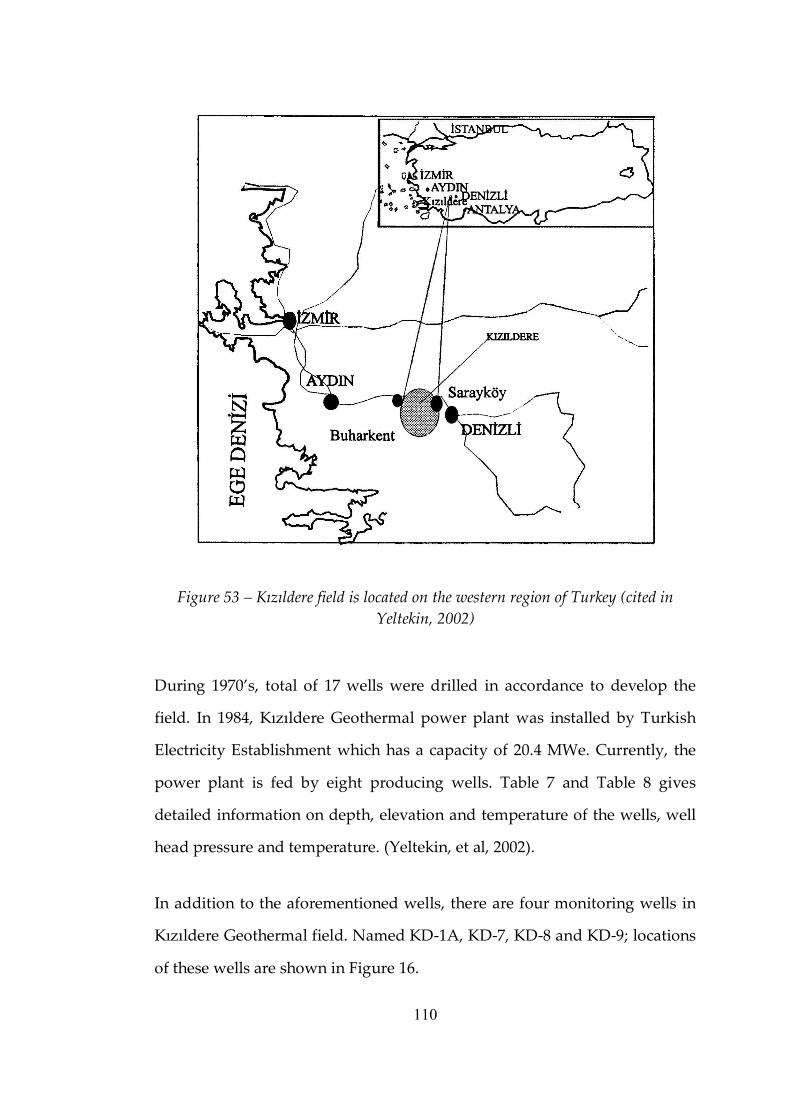
110
Figure 53 – Kızıldere field is located on the western region of Turkey (cited in Yeltekin, 2002)
During 1970’s, total of 17 wells were drilled in accordance to develop the
field. In 1984, Kızıldere Geothermal power plant was installed by Turkish
Electricity Establishment which has a capacity of 20.4 MWe. Currently, the
power plant is fed by eight producing wells. Table 7 and Table 8 gives
detailed information on depth, elevation and temperature of the wells, well
head pressure and temperature. (Yeltekin, et al, 2002).
In addition to the aforementioned wells, there are four monitoring wells in
Kızıldere Geothermal field. Named KD‑1A, KD‑7, KD‑8 and KD‑9; locations
of these wells are shown in Figure 16.
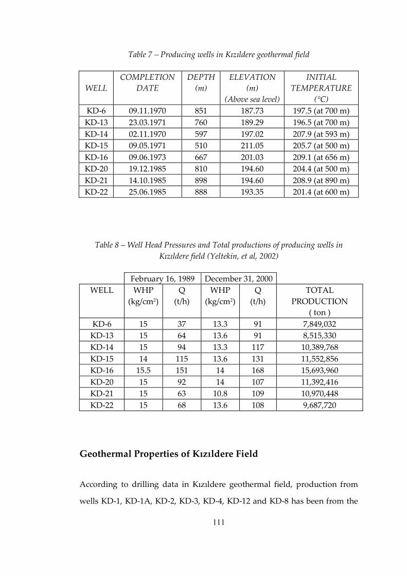
111
Table 7 – Producing wells in Kızıldere geothermal field
WELL COMPLETION
DATE DEPTH (m)
ELEVATION (m)
(Above sea level)
INITIAL TEMPERATURE
(°C) KD‑6 09.11.1970 851 187.73 197.5 (at 700 m) KD‑13 23.03.1971 760 189.29 196.5 (at 700 m) KD‑14 02.11.1970 597 197.02 207.9 (at 593 m) KD‑15 09.05.1971 510 211.05 205.7 (at 500 m) KD‑16 09.06.1973 667 201.03 209.1 (at 656 m) KD‑20 19.12.1985 810 194.60 204.4 (at 500 m) KD‑21 14.10.1985 898 194.60 208.9 (at 890 m) KD‑22 25.06.1985 888 193.35 201.4 (at 600 m)
Table 8 – Well Head Pressures and Total productions of producing wells in Kızıldere field (Yeltekin, et al, 2002)
February 16, 1989 December 31, 2000 WELL WHP
(kg/cm 2 ) Q (t/h)
WHP (kg/cm 2 )
Q (t/h)
TOTAL PRODUCTION
( ton ) KD‑6 15 37 13.3 91 7,849,032 KD‑13 15 64 13.6 91 8,515,330 KD‑14 15 94 13.3 117 10,389,768 KD‑15 14 115 13.6 131 11,552,856 KD‑16 15.5 151 14 168 15,693,960 KD‑20 15 92 14 107 11,392,416 KD‑21 15 63 10.8 109 10,970,448 KD‑22 15 68 13.6 108 9,687,720
Geothermal Properties of Kızıldere Field
According to drilling data in Kızıldere geothermal field, production from
wells KD‑1, KD‑1A, KD‑2, KD‑3, KD‑4, KD‑12 and KD‑8 has been from the

112
first reservoir rock of Pliocene limestones (Şimşek, 1985). KD‑6, KD‑7, KD‑9,
KD‑13, KD‑14, KD‑15, KD‑16, KD‑20, KD‑21, KD‑22 wells are bearing
second reservoir (İğdecik formation), cutting through sandstones instead of
limestones. The thickness of the second reservoir varies between 100 and 300
m. When compared to the first reservoir rock, the second has relatively high
secondary porosity and permeability combine with lateral continuity
making it suitable for secondary recovery techniques such as water injection.
Water Source
Water supply of the field is mainly from precipitiation and from surface and
underground water that flow into the basin through the major faults. After
being heated in greater depths, water travels upwards to the reservoir
through these bounding faults (Figure 54).
Figure 54 – Water migration paths of Kızıldere geothermal Field (Yeltekin, et al 2002)

113
Reservoir Pressure
In Kızıldere geothermal field aforementioned observation wells are used to
constantly monitor the reservoir pressure. Reinjection of waste water back to
the reservoir is the only solution to prevent the depletion of reservoir
pressure. A reinjection project was prepared for this purpose in 1995 and
MTA drilled 3 reinjection wells during the period 1996 and 2000. One of
these wells is in the Tekkehamam area 3 km away and the others are near
the Kızıldere Geothermal field. The well drilled in Tekkehamam (TH‑2) is
not suitable for reinjection because of low injectivity. The first reinjection
well drilled in Kızıldere area (R‑1) resulted with a high production capacity
but low injectivity. It has a temperature of 243 °C and it is the best producer
of Turkey. Its capacity is 6 Mwe. The second well drilled in Kızıldere area
(R‑2) showed good injectivity as well as good production capacity. It is
planned to start reinjection from R‑2 by the end of 2001. (Yeltekin, et al,
2002).


![International Journal of Engineering RESEARCH · carbonate oil reservoirs [15-17] is their natural fracture networks. Oil is mainly stored in these fractured carbonate reservoirs](https://img.pdfslide.net/doc/110x75/5f237153f145bd1f082637d4/international-journal-of-engineering-carbonate-oil-reservoirs-15-17-is-their-natural.jpg)