Embed Size (px)
Citation preview
Optimized Photogrammetric Network Design with Flight Path Planner
for UAV-Based Terrain Surveillance
Ivan Y. Rojas
A thesis submitted to the faculty ofBrigham Young University
in partial fulfillment of the requirements for the degree of
Master of Science
John D. Hedengren, ChairRyan M. FarrellWilliam G. Pitt
Department of Chemical Engineering
Brigham Young University
December 2014
Copyright © 2014 Ivan Y. Rojas
All Rights Reserved

ABSTRACT
Optimized Photogrammetric Network Design with Flight Path Plannerfor UAV-Based Terrain Surveillance
Ivan Y. RojasDepartment of Chemical Engineering, BYU
Master of Science
This work demonstrates the use of genetic algorithms as a stochastic optimizationtechnique for developing a camera network design and the flight path for photogrammetricapplications using Small Unmanned Aerial Vehicles. This study develops a Virtual Optimizerfor Aerial Routes (VOAR) as a new photogrammetric mapping tool for acquisition of imagesto be used in 3D reconstruction.
3D point cloud models provide detailed information on infrastructure from placeswhere human access may be difficult. This algorithm allows optimized flight paths to monitorinfrastructure using GPS coordinates and optimized camera poses ensuring that the set ofimages captured is improved for 3D point cloud development. Combining optimizationtechniques, autonomous aircraft and computer vision methods is a new contribution thatthis work provides.
This optimization framework is demonstrated in a real example that includes retriev-ing the coordinates of the analyzed area and generating autopilot coordinates to operate infully autonomous mode. These results and their implications are discussed for future workand directions in making optical techniques competitive with aerial or ground based LiDARsystems.
Keywords: UAV, flight planner, optimization, terrain surveillance, photogrammetry, remotesensing, Ivan Rojas

ACKNOWLEDGMENTS
To my parents, Eva and Guillermo Rojas, for their constant support, for always
encouraging me to give my very best, for motivating me to pursue higher education, and
for providing the means and resources to reach this point. My siblings deserve my whole-
hearted thanks as well. I also express my appreciation to my fiance for all her support, time,
comprehension and especially her love throughout the whole process.
I express deepest gratitude to my thesis advisor, Dr. John D. Hedengren, for trusting
me and permitting me to work as part of his team. From the very beginning, his support and
his technical guidance has led me to develop the scientific abilities necessary to accomplish
this project and gain meaningful experience by presenting at conferences in the NASA Lan-
gley Research Center, the University of Colorado Boulder, and Snowbird Utah. Likewise,
I appreciate Dr. Ryan M. Farrell for his contributions in Computer Vision, his dedication
in teaching me computer science and programing languages, but most importantly, for his
influence in my personal life through his righteous example of leading a balanced life. Fi-
nally, I would like to acknowledge Dr. William G. Pitt for always being aware of my progress
and offering his sincere help from the time I began the graduate program until the end of
this project; he helped me to recall important engineering principles from my undergraduate
studies that were essential in earning this degree.
Special thanks to all the team members involved in this project. Abraham Martin
formulated the original idea for this project and introduced me to it. Colter J. Lund con-
tributed civil engineering expertise and worked as an always-smiling friend; without him,
this project would not have been possible. Brandon L. Reimschiissel was always willing to
keep the fleet ready to fly and had excellent flying skills; his ability to integrate me into the
group was significant and his friendship was especially sincere.

Also, I thank my colleague, Edris Ebrahimzadeh, for sharing his outstanding abilities
in Matlab and being willing to explain difficult chemical engineering concepts. His help has
been invaluable. Hector D. Perez contributed the development of the fitness function, his
collaborative attitude, and his friendship. Lastly, I would like to recognize the members of
the UAV group in the PRISM lab, Zack Romero, Joshua Pulsipher and Joseph Clark for
their constant support.
In memory of Israel D. Worthington (1987-2014), a brilliant young scientist and my
greatest friend.
Table of Contents
List of Tables xi
List of Figures xiii
1 Introduction 1
2 Background 5
2.1 Infrastructure Spatial Sensing . . . . . . . . . . . . . . . . . . . . . . . . . . 5
2.2 Data Collection and Aerial Route Optimization . . . . . . . . . . . . . . . . 9
3 Multi-objective Optimization 13
3.1 UAV and Photogrammetry . . . . . . . . . . . . . . . . . . . . . . . . . . . . 14
3.2 Camera Location and Orientation . . . . . . . . . . . . . . . . . . . . . . . . 16
3.3 Fitness Function . . . . . . . . . . . . . . . . . . . . . . . . . . . . . . . . . 20
3.4 Flight Path Planning . . . . . . . . . . . . . . . . . . . . . . . . . . . . . . . 23
4 Laboratory Validation 29
4.1 Iterative Closest Point and Ray Tracing Algorithm . . . . . . . . . . . . . . 29
4.2 Methodology . . . . . . . . . . . . . . . . . . . . . . . . . . . . . . . . . . . 29
4.3 Results . . . . . . . . . . . . . . . . . . . . . . . . . . . . . . . . . . . . . . . 31
5 Field Trial Validation 37
5.1 Multi Objective Optimization . . . . . . . . . . . . . . . . . . . . . . . . . . 37
v

5.2 Qualitative Analysis . . . . . . . . . . . . . . . . . . . . . . . . . . . . . . . 38
5.3 Quantitative Analysis . . . . . . . . . . . . . . . . . . . . . . . . . . . . . . . 40
6 Optimization Under Different Scenarios 47
6.1 Privacy Assurance . . . . . . . . . . . . . . . . . . . . . . . . . . . . . . . . 47
6.2 Planning and Simulation . . . . . . . . . . . . . . . . . . . . . . . . . . . . . 48
6.3 Flight Test . . . . . . . . . . . . . . . . . . . . . . . . . . . . . . . . . . . . . 49
7 Conclusion and Future Considerations 53
Appendix A Genetic Algorithm Source Code 57
Bibliography 91
vi

List of Tables
3.1 Genetic Algorithm Parameters . . . . . . . . . . . . . . . . . . . . . . . . . . 24
4.1 95% Confidence Interval Quality Assessment Results . . . . . . . . . . . . . 33
5.1 95% Confidence Interval Quality Assessment Results . . . . . . . . . . . . . 43
6.1 Privacy Protection Results . . . . . . . . . . . . . . . . . . . . . . . . . . . . 50
vii
List of Figures
2.1 Camera locations in a 3D point cloud . . . . . . . . . . . . . . . . . . . . . . 7
2.2 Example of 3D triangulation. . . . . . . . . . . . . . . . . . . . . . . . . . . 8
2.3 Example of a 3D model developed with SfM . . . . . . . . . . . . . . . . . . 9
3.1 Dimensions of an image formed in the camera given a focal length . . . . . . 16
3.2 Flow chart of camera network and flight planning optimization . . . . . . . . 17
3.3 Resolution of 3 different sensors . . . . . . . . . . . . . . . . . . . . . . . . . 19
3.4 Frustum of camera surveying space . . . . . . . . . . . . . . . . . . . . . . . 19
3.5 Example of feature detection in the spatial and frequency domain. . . . . . . 21
3.6 Example of SIFT features extraction . . . . . . . . . . . . . . . . . . . . . . 22
3.7 Generation improvement over the time . . . . . . . . . . . . . . . . . . . . . 24
3.8 Comparison in elevation standard grid and optimized waypoints . . . . . . . 25
3.9 Representation of an optimized flight path . . . . . . . . . . . . . . . . . . . 27
4.1 Diagram of the ray tracing technique . . . . . . . . . . . . . . . . . . . . . . 30
4.2 Iterative closest point measurements . . . . . . . . . . . . . . . . . . . . . . 31
4.3 Laboratory validation . . . . . . . . . . . . . . . . . . . . . . . . . . . . . . 32
4.5 95% Confidence interval accuracy using Nikon DSLR . . . . . . . . . . . . . 33
4.4 Computer generated 3D models for laboratory validation . . . . . . . . . . . 34
5.1 Aerial view of the study case area . . . . . . . . . . . . . . . . . . . . . . . . 37
viii

5.2 First and last generation of the camera location optimization . . . . . . . . 39
5.3 Generation improvement over the time . . . . . . . . . . . . . . . . . . . . . 40
5.4 Field validation results using standard grid planning . . . . . . . . . . . . . . 41
5.5 Field validation results using VOAR . . . . . . . . . . . . . . . . . . . . . . 42
5.6 95% confidence interval of the field test . . . . . . . . . . . . . . . . . . . . . 43
5.7 Flight path resulting from the optimization . . . . . . . . . . . . . . . . . . . 44
5.8 Optimized way points . . . . . . . . . . . . . . . . . . . . . . . . . . . . . . . 45
6.1 Representation of a reward and penalty map in a privacy approach . . . . . 48
6.2 Test area and privacy areas . . . . . . . . . . . . . . . . . . . . . . . . . . . 49
6.3 Planned flight path . . . . . . . . . . . . . . . . . . . . . . . . . . . . . . . . 50
6.4 Quadcopter used for this study . . . . . . . . . . . . . . . . . . . . . . . . . 51
6.5 Private sectors . . . . . . . . . . . . . . . . . . . . . . . . . . . . . . . . . . . 51
6.6 Actual flight path . . . . . . . . . . . . . . . . . . . . . . . . . . . . . . . . . 52
ix

Chapter 1
Introduction
Unmanned Aerial Vehicles (UAVs), commonly known as “drones” [1] provide promis-
ing applications in many fields and are providing increasingly valuable services to industry.
Although historically UAVs have been used largely in military applications, new industrial
opportunities [2] may utilize UAVs as remote sensing tools in areas such as infrastructure
monitoring due to their autonomous nature and non-intrusive capabilities.
UAVs development has been rising in recent years. Coupled with parallel technologies
like camera capabilities (such as size, quality, sensitivity or GPS precision) and new computer
vision techniques [3], the breakthroughs offer a number of high-impact use cases [4].
One of the recent applications in which new capabilities are being explored [5] is
maintaining functionality of facilities or public infrastructure. According to the National
Science Foundation, restoring and improving urban infrastructure was included as one of the
21st century’s grand Engineering challenges [6].
In this way, one of the recent applications in which UAVs have demonstrated ad-
vantages over traditional methods is in performing photogrammetry surveillance. Current
available information obtained from satellites is limited to 10 cm resolution [7]. In con-
trast, UAV based surveillance methods can provide 1-5 cm resolution compared with ground
sample distance (GSD) [8] [9] [10].
Tools such as the Scale Invariant Feature Transform (SIFT) feature detector and
Structure from Motion (SfM) algorithms [11] make it possible to use a series of overlapping
photographs to create three dimensional models of any terrain or scene. These models provide
detailed information of places that may be difficult to survey or monitor by conventional
terrestrial methods. Whether for orthophoto reconstruction [12], accurate 3D infrastructure
1

monitoring [13] or any other application in which centimeter resolution is preferred, UAV
based collection may enhance the productivity of the resulting models.
Common methods [14] for UAV image capture are through manual or arbitrary cap-
ture methodologies. Photogrammetric capture is facilitated by ground station software that
may generate a grid flight pattern that includes image overlap. These methods may yield in-
complete or inferior models. In spite of the cost efficient image acquisition, one of the biggest
constraints that this technique is facing is the limited flight time of the UAV. Currently the
average flight time of a small UAV multicopter is in the range of ten to thirty minutes for
battery powered platforms. This work optimizes both the location and flight path of the
UAV to maximize the information content of the acquired photographs.
Chapter 2 provides a review of spatial sensing including characteristics of different
sensors and the techniques for 3D reconstruction. Prior work in optimizing UAV flight paths
to achieve improved models is also discussed.
Chapter 3 presents an outline of optimization and different techniques used in en-
gineering to solve multi-objective problems and applications of aerial photogrammetry, in-
troduces computer vision principles for the development of 3D models and applies such
principles in a mathematical system to plan an optimized flight path in order to meet the
objective of a detailed 3D point cloud.
Chapter 4 discusses a ray tracing technique and an iterative closest point algorithm as
a foundation to develop a preliminary laboratory experiment. In this experiment, an object
is placed in the middle of a grid to obtain an optimized network camera and develop a 3D
model and perform a quality assessment.
Chapter 5 sketches a field evaluation in a representative site that shares similar fea-
tures to chemical plants and representative structures used in the industry. This field eval-
uation shows the efficiency of the methods and the applicability as a general solution. The
results and accuracy are quantified in demonstrating improved performance with optimiza-
tion.
2

Chapter 6 introduces a novel approach for terrain surveillance under a different sce-
nario in which public privacy is taken into account as a primarily consideration. A reward
map is develop for the areas of importance and a penalty map for areas which should be
avoided.
In summary, this study introduces a system that maximizes the photographic coverage
and minimizes the number of locations in which pictures need to be taken in order to find
the shortest, most efficient aerial route that best utilizes flight time.
3

Chapter 2
Background
2.1 Infrastructure Spatial Sensing
Using remote optical sensing for maintaining the functionality of facilities and public
infrastructure has been increasingly embraced due to the host of benefits that it offers, such
as the detailed qualitative and quantitative information it provides. This data facilitates the
ability to analyze the condition of such infrastructure and implement critical preventive or
corrective maintenance. The often smalls sensors can reach places that would otherwise be
dangerous or inaccessible with traditional methods.
In practice, optical-based sensors can be classified as either active or passive, de-
pending on whether the sensor transmits or receives energy [15], While passive sensors only
receive the light reflected by an external source, active sensors emit a light or other source
to interrogate the structure.
Terrestrial laser scanners work under the principle of time-of-flight (TOF) in which
the distance between the instrument and the object or landscape is measured by the time
that takes for a pulse or laser beam to hit the surface and bounce back to the instrument.
Light Detection and Ranging (LiDAR) sensors send out pulses, record measurements and
build up the shape of the terrain or landscape with millimeter level resolution [16]. It is not
affected by natural light and offers the advantage that it can be used both during the day
or night.
Nevertheless, LiDAR has downsides such as the mixed-pixel effect [17] in which the
reflected beam is separated by long distances. This usually happens with points close to
4

edges onto sufaces with diferent distances from the sensor. Known as the Multipath effect
[18], the target distance falsely increases due to reflection on surrounding objects.
Another disadvantage of LiDAR is that data is typically collected from multiple loca-
tions along the landscape, using fixed controls as references. Several point clouds are merged
to create the whole scene. The main disadvantages of LiDAR techniques are the high cost of
the equipment, model processing, and information extraction from large point cloud models.
In contrast to active sensors such as LiDAR, passive sensors are less expensive, depend
on an external source of light, and offer faster surveying. However the quality of the results
relies largely on the resolution of the sensor and on the post-processing algorithms used to
develop the 3D model. One of the most common is Structure from Motion (SfM) which is
defined by Szeliski [19] as:
“Estimating the locations of 3D points from multiple images given only a sparse set
of correspondences between image features. While this process often involves simultaneously
estimating both 3D geometry (structure) and camera pose (motion), it is commonly known
as structure from motion”.
The idea of a flip book was one of the first principles that lead to the current SfM
algorithm. In a flip book, pages are flipped for a set interval enabling a perception of move-
ment to the human eye. In 1979, Ullman [20] used this idea to define the rigidity assumption
as any set of elements undergoing a two dimensional transformation which, having a unique
interpretation as a rigid body moving in space should be interpreted as a body in motion.
These assumptions, combined with the Johansson’s observation [21] in 1964 that rigid-
ity plays a special role in motion perception, produced the Structure from Motion theorem
[20]:
“Given three distinct orthographic views of four non-coplanar points in a rigid config-
uration, the structure and motion compatible with the three views are uniquely determined.”
5

Having these three views, the pose of a given set of cameras can be estimated. This
process is often known as alignment or the perspective-3-point-problem (P3P) [22] and relies
on the observation that the visual angles and distances between a pair of 2D points must be
the same as the angle between their corresponding 3D points.
Once these distances and angles are computed, the structure can be generated as a
3D point cloud with respective point directions and orientation from different techniques
[23]. An example of a set of camera locations and the generated point cloud can be seen in
Figure 2.1.
(a) 2D and 3D view of a given camera andthe location in the 3D point cloud
(b) View of a set camera locations in a 3Dpoint cloud
Figure 2.1: A photogrammetry software called RealityCapture [24] provided by companyCapturing Reality s.r.o. was used to compute camera calibrations and a sparse point cloud.
When these views are obtained via orthographic projection, the 3D structure can be
recovered from as few as four points in three views. This is the minimal requirement to
obtain a unique representation of all points in a 3D projection [25].
Figure 2.2 illustrates the process of determining a point 3D position from correspon-
dences in camera locations. This process is known as triangulation; the positions of multiple
points are located from three pictures taken from different locations at possibly different
times and by matching the 2D feature locations.
6

Figure 2.2: Example of 3D triangulation. Images: Ryan Farrell CC - jdegenhardt, BobSnyder, Jacques van Nierkerk, Kyle Wagaman, (Flickr)
A method for reconstruction that is used in this work is an open source program
called CMPMVS [26], which is a platform for reconstructing outdoor surfaces or landscapes
where the background may be out of focus and hence blurry (weakly supported). It starts
the 3D reconstruction process by generating a 3D point cloud from depth-maps followed by
a Delaunay tetrahedralization and labeling the tetrehedra as occupied. Such modification
allows the reconstruction of weakly supported surfaces.
LiDAR or Photogrammetry offer advantages and disadvantages, depending on the
scope of the analysis, the use of the data obtained, and the budget involved. Both are
widely used for collecting spatial information. This study is intended to show that with
the use of optimization and computer vision techniques, the accuracy of computer vision
techniques can approach the accuracy of LiDAR and exceed terrestrial LiDAR for overall
surface coverage.
7

(a) Aerial view of a cliff (b) View of the 3D model
(c) Aerial view of a geological formation (d) Close up to the 3D model
Figure 2.3: Example of a 3D model developed with SfM
2.2 Data Collection and Aerial Route Optimization
Another variable that plays an important role in the development of 3D models is the
quality of the set of pictures. In this particular case it refers to the number of points that
are seen at least three times to satisfy the SfM theorem. Manual or arbitrary image capture
methods may yield incomplete models of poor quality. Optimization of the UAV flight path
improves both the accuracy and resolution of the 3D model. This is accomplished by se-
lectively choosing location and pose information for the image capture to maximize metrics
that are desirable for 3D model construction, resolution and accuracy.
To tackle this problem, a multi-objective optimization approach is used. Among the
variety of optimization techniques, there is a special group known as Heuristic methods.
Heuristics [27] are a custom procedure to search for a solution; even when the optimal
solution is not guaranteed, the result is often close enough to the global optimum.
8

A special kind of Heuristic technique is the Metaheuristic which is defined [28] as:
“Methods that can be applied to a wide set of different problems. In other words, a meta-
heuristic can be seen as a general algorithmic framework which can be applied to different
optimization problems with relatively few modifications to make them adapted to a specific
problem. ”
The metaheuristic search strategies are subdivided according to functionality into:
� Population evolutionary
� Intelligence gradual construction
� Neighbourhood search
� Relaxation
Heinonen and Pukkala [29] compared multi-objective optimization using heuristic
optimization techniques, and concluded that Genetic Algorithms perform best as applied to
spatial problems. While Genetic Algorithms have been used previously on spatial problems,
including UAV flight planning, there are no prior photogrammetric applications. The typical
ten to thirty minute flight time of the battery-powered UAV limits the picture capture
process. The limited flight time leads to another problem to solve: the optimal flight path.
With camera path optimization, the UAV has a set of coordinates that are visited to
meet the objective of data collection for the 3D model rendering. This situation can be seen
as an instance of the traveling salesman problem (TSP), a classic combinatorial optimization
problem which has been widely studied for over 30 years [30].
There exist multiple methods which can be applied to produce approximate solutions
to this non-deterministic polynomial-time hard (NP-hard) problem. Olafsson [31] gives some
examples that are the most commonly used to address complex optimization problems: sim-
ulated annealing (SA), tabu search (TS), iterated local search (ILS), evolutionary algorithms
(EA), and ant colony optimization (ACO).
9

Tabu search is a technique that solves optimization problems based on managing
a multilevel exploration and memory. It uses the concept of a neighborhood to try solu-
tions constraining the system to break up the last movements. This forces the search in
environments that otherwise wouldn’t be explored. In spite of being a good approach, this
research is intended to use other metaheuristic algorithms, such a genetic algorithms and
its variations, to find a suitable solution. One of the most useful characteristics of Genetic
Algorithms is the mutation probability which combines the current best solution with the
exploration of new search space, this being a combination of stochastic and directed search
[32]. For instance Qu, Pan and Yung [33] used a genetic algorithm for UAV flight planning
showing that they are one of the most suitable optimization methods for this application.
A few previous applications [34] of aerial route optimization have been considered.
For instance, the first use of Aerial photography of a village close to Paris by Tournachon
[35] was in 1958 with a hot-air balloon. The first attempts at using UAVs took place in
1979 when Przybilla and Wester-Ebbinghaus [36] did the first experiments with a small Hegi
airplane in Germany. Later on, in 2004 Eisenbeiss [13] used a helicopter with a flight planner
and autopilot to fly over a mining terrain of 200×300 m in Peru, also with the future intend
to develop a 3D model and compare it with a laser-based model, and more recently in 2012
with aerial triangulation [37]. Nevertheless, none of those previous approaches have the
current objective of minimizing camera locations and maximizing coverage for optimal 3D
models. This work is the first known study to develop optimized photogrammetric methods
for maximizing final model quality with minimized flight time.
10

Chapter 3
Multi-objective Optimization
When solving engineering problems, one frequently encounters comparative words
such as maximum, minimum, more, or less. These words seek to pinpoint the optimal
solution to a problem. Pursuing the best solution or, in other words, finding the most
cost-effective [38] solution for a problem can be defined as optimization. However, in an
engineering context, the costs are not necessarily monetary, but can also come in the form
of time, materials, length, distance, and many other factors. Combining multiple factors in
one optimization problem creates a multi-objective problem that trades-off between the best
combination of desirable outcomes.
Several optimization techniques have been developed for different purposes. Certain
techniques may apply in some instances, but may not apply in others. For instance, it is
necessary to maximize resistance and minimize weight when designing a civil structure such
as a bridge. A particular technique may identify a way to optimize both constraints with a
particular design, while another technique may develop a distinct design that also satisfies
the requirements. The optimal design among all those possible solutions is known as the
global optimum, whereas the set of possible solutions represents the feasible space.
Exact methods (gradient based) are meant to find a good approximation to the global
optimum by not only satisfying the given constraints, but also verifying that result after-
wards [38]. The heuristic search method starts with a previously given solution and examines
the surrounding for a better solution. These methods perform well in multi-objective opti-
mization and encompass another subdivision of methods called Metaheuristics.
11

The following diagram provides a classification [38] of the global optimization meth-
ods:
Global methods
Exact methods Heuristic search methods
Metaheuristics
Scatter search Tabu search Simulated annealing Genetic and evolutionary
Metaheuristics utilize the advantages of heuristics by examining a nearly global ap-
proximation of the surroundings. However, in order to avoid settling for local optimum
results, these methods offer the advantage of honing this search by changing the parameters
in the algorithm and exploring other neighborhoods. This is by far one of the most suitable
techniques for situations in which multiple criteria have to be met simultaneously, and which
have a risk of finding local optima.
This study uses Metaheuristics to find the global optimal solution. Genetic algo-
rithms are named after the biological likeliness of optimizing biological processes where a
pair of chromosomes can mutate and cross over in order to improve the next generation.
Since heuristic techniques start the search for the optimum with a given solution, a first
generation should be provided. Further detail regarding genetic algorithms and the require-
ments for this case study will be discussed in the following sections.
3.1 UAV and Photogrammetry
Unmanned Aerial Vehicles (UAVs) trace their roots as far back as 1916 for military
operations [39]. The decreasing cost and increasing reliability of these versatile aircrafts have
12

opened up new possibilities for several domestic uses, such as geological surveying [40], nat-
ural disaster monitoring [41], fighting forest fires, monitoring wildlife populations, assisting
in rescue operations following disasters [42], or spreading fertilizer. For instance, in Japan,
at least 10 percent of all sprayed paddy fields are sprayed by unmanned helicopters [39].
In the field of chemical engineering, UAVs have been used for an increasingly wide
array of purposes, such as monitoring gas pipelines. Although this particular application
is still in its early stages, UAVs have great potential when used to monitor pipelines for
potential leaks [43] and to prevent disasters.
Many studies [44] have combined the versatility of UAVs and the advantages of pho-
togrammetry. Relatively few, however, have included computer vision techniques and 3D
model development for surveying terrain and monitoring infrastructure. Combining these
three branches of science provides a useful alternative to the classic remote sensing approach.
For example, it is available at a lower cost and offers faster information acquisition without
sacrificing the accuracy of the final results. In fact, this particular combination of techniques
can approach the precision of laser-based sensors.
Because UAVs are able to capture images from a distance, one of the main advantages
of remote UAV-based sensing is the capability to reach places that would otherwise be
inaccessible to terrestrial scanning devices. Equation 3.1 is used to calculate the distance at
which a UAV camera sensor should be positioned from the target.
h = Hf
d(3.1)
In this equation, f is the focal length, h is the camera sensor height,d is the distance
from the sensor to the far plane and H is the height of the far plane of the frustum. To
illustrate this important equation, an example of a camera taking an aerial picture of a ge-
ological formation is shown in Figure 3.1.
13

Figure 3.1: Dimensions of an image formed in the camera given a focal length
One main element in the image acquisition is the distance from the sensor to the
object of interest because this distance determines the resolution of the final model. The
purpose of this study is that each pixel on a picture corresponds to a 0.5 cm of geological
structures or infrastructure such as pipelines and levees. This condition is also affected by
the number and density of camera locations (pictures) in the chosen area; A synthetic ex-
periment is developed in Chapter 4 to further illustrate this principle.
After defining the optimal number and location of waypoints as well as the orienta-
tion of each camera, the next step is to determine the order of the waypoints. This study
is intended to optimize the order in which these waypoints are visited in order to conduct
a completely autonomous UAV mission and collect images that are ultimately used to pro-
cess the final 3D point cloud model. Figure 3.2 represents the workflow that guides this study.
3.2 Camera Location and Orientation
Several variables and sets of constraints are applied simultaneously in the process
of adjusting each camera to find the optimal coordinates (latitude and longitude), position
(tilt, pitch, roll), distance to the ground (altitude), and optimal flight path. Given the na-
ture of the problem, it is difficult, or even impossible, to develop an equation and combined
constraints (model) as is required for the use of an exact method.
14

Figure 3.2: Flow chart of camera network and flight planning optimization
Genetic algorithms are considered a robust technique since they offer a global opti-
mum by utilizing different objectives and boundary conditions concurrently, directing this
search out of the feasible space. This outstanding method is also known as an “adaptative”
[45] or “evolutionary” genetic algorithm [46] technique. This proposed general solution has
proven to be efficient for various kind of infrastructure or terrain surveillance in this type of
spatial optimization problem [47].
Without loss of generality, the area (polygon) of interest is selected and converted
into a Keyhole Markup Language, which is a tag-based format developed in XML to display
geographic data in an Earth Browser [48]. This particular format includes the longitude and
latitude information of such a polygon. Nevertheless, the mode in which the information is
gathered ignores the altitude value (clamp to ground); therefore, this missing information
needs to be obtained from a secondary source.
One of the public sources from which this information can be obtained is the fed-
eral agency in charge of providing geography and geology information, the United States
Geological Survey (USGS). Other entities, such as the National Aeronautics and Space Ad-
ministration (NASA), is another source of this data. The purpose of this granular elevation
data is to optimize the location and pose information of the camera. As the model is refined,
the optimization solution is improved.
15

The computational platform in which this research is developed is Matlab. After
selecting the area of interest, the algorithm looks for the edges of the polygon, and based on
these coordinates (latitude and longitude) the altitude is extracted.
Based on a previous approach introduced by Niedfeldt et al. [49], the algorithm loads
the latitude, longitude and elevation of the terrain and plots them into a point cloud. Next,
the trial points (population) are selected by setting random camera locations in the space
above the terrain point cloud. Because a resolution of 0.5 cm per pixel is expected, the
distance from the camera locations to the terrain is also considered.
Various sensors (cameras) are utilized in this study. Consequently, the maximum
distance for a given camera was computed using Equation 3.1 in order to achieve the desired
resolution, and the results are shown below in Figure 3.3. Points beyond this distance are
considered invisible to the camera. This set of camera locations and poses yields information
with positions and orientations, which are adjusted to maximize the quality of the image
mapping during the UAV surveying flight.
The functional coverage is defined as the ratio of the area covered by the set of cameras
to the area to be reconstructed. In order to determine the area covered by a given set of
cameras, a viewing space (frustum) for each camera is defined according to geographical
position and the distance from the camera to the far plane, as seen in Figure 3.4
.
The model determines which points are in the frustum threshold by using Equa-
tion 3.1 and provides the dot product between the normal of the frustum and the terrain
points. The terrain points that are visible to each individual camera are determined by an
occlusion test developed by Katz [50]. This test involves reflecting the point cloud in the
frustum onto a spherical surface away from the camera. Any points that are not reflected
are not included in the frustum; However, the entire set of visible points is included, as
seen in Figure 3.4(a). After simulating real conditions, the real-valued genetic algorithm
16

0 5 10 15 20 25 30 35 40 45 500
20
40
60
80
100
120
140
160
180
200
Resolution per pixel(mm)
Dis
tanc
e to
the
goru
nd (m
)
Go Pro 2 MpGo Pro 12 MpNikon 24 Mp
Figure 3.3: Comparison in resolution for 3 sensors, Gopro Hero 3 black edition in cameraand video mode and a DSLR Nikon D7100
(a) Frustum of camera surveying space (b) Example of reflecting points on a surfacefor occlusion testing
Figure 3.4: Example of Frustum and occlusion test on camera surveying space
finds the camera collocation that maximizes the quality of the image mapping. Once this
camera location and orientation is established, an initial population is randomly generated
and scored. The criteria for which the first solution is evaluated is called the fitness function.
17

3.3 Fitness Function
The fitness function is based upon the SfM algorithm that generates 3-dimensional
structures from a 2 dimensional set of images. One of the main functions of this computer
vision technique is the use of features and object recognition. The method utilized by CMP-
MVS is the Scale Invariant Feature transform (SIFT), which identifies the key features in
each image by looking for the maximum and minima of differences within a Gaussian func-
tion [51].
These key features are then converted into vectors that portray the region sampled
and saved in a database. The key features are invariant to scaling and rotation, and only
partially variant to brightness and angles, in both the spatial and frequency domains. As a
result, when another picture is analyzed, every key feature is compared to the information
saved in the database, resulting in virtually no disruption [52]. The low degree of disruption
allows for the reconstruction of the exact 3D position [25]. Figure 3.6 illustrates the extrac-
tion of a sample of the key features by SIFT.
When a set of pictures overlaps poorly [53], the SIFT extraction has a lower proba-
bility of finding the exact 3D position of each point. Therefore, a pairwise overlap of 50%
[54] to 80% [55] between images is desirable [56]. Each point should not only be imaged by
several cameras, but also from different angles [57].
To accomplish this, and in order to provide diversity, the space is divided into five
sections based on the azimuth sectors of 72 degrees each, giving priority to designs with
camera positions in at least three of the five regions. This requirement meets the objective
of having each terrain point appear in at least three cameras and allows images to be captured
from diverse angles. The maximum distance from the camera to the terrain is also counted
towards the score of the final evaluation of the proposed solution, as seen in Equation 3.2
f =n∑
i=1
(Ni − 2) +n∑
i=1
5∑j=1
Tij (3.2)
18

(a) Initial position of the box (b) Box rotated
(c) Key features (Corners) in the spatial do-main
(d) Features detection in the object rotated
(e) Box in the frequency domain (f) Main features in the frequency domain
Figure 3.5: Example of feature detection in the spatial and frequency domain.
In this equation, N is the number of cameras capturing the point i at n points of the
terrain, and T is the score given for the presence of at least one camera in each j region. The
first term evaluates the number of cameras capturing the given point, and the second term
19

(a) Image of a mountain
(b) SIFT features extraction
Figure 3.6: Example of SIFT features extraction
evaluates the point being seen from different angles. The score assigned is used to encourage
design improvement after each generation.
Position and orientation data (population) is randomly generated and scored by the
fitness function for an initial set of cameras. Following the principles of the survival of the
fittest, the highest scores from each generation are meant to compete. This process is known
as tournament, and the best scores are chosen as the “mother” and, similarly, the “father”.
In order to ensure an improved new generation over the time, a tournament selection size of
four is selected throughout the iteration of generations. These parents are mixed to create
two children using blend crossover. Crossover is an operator of the genetic algorithm that
combines the two parents in order to improve them so the evolution process can continue.
Blend crossover takes into account Equations 3.3a and 3.3b, where C1 and C2 are children
and P1 and P2 are parents, the weighted average of the positions along the 3 axes (x,y,z ),
and the camera orientation (tilt and roll).
20

In these equations, a is a random number between 0 and 1. This process is carried
out as often as determined by the crossover probability. Because a high [7] rate of crossover
probability is desirable when solving NP-complete problems, a rate of 90% has been selected.
C1 = P1 + a(P1 − P2) (3.3a)
C2 = P2 − a(P1 − P2) (3.3b)
Another operator used in genetic algorithms is mutation, which helps the algorithm to
overcome local maxima by introducing new individuals into the population, providing diver-
sity to future generations. Although mutation helps in the early stages of optimization, this
probability should decrease as new generations are created in order to refine the search and
save computational effort. This process is called dynamic mutation and randomly changes
the genes of the children. This mutation rate was applied to the three axis positions and
to the camera orientation. Furthermore, some parameters were initially modified randomly
within the variable bounds and this magnitude decreased throughout the optimization.
After studying different schemes [58] and by conducting repeated simulations, the
parameters shown in Table 3.1 were implemented in the genetic algorithm. As would be
expected, the increased number of cameras locations led to a better solution at the cost of
additional computation time.
Through empirical observation and the use of the previously mentioned parameters,
Figure 3.7 shows that around 20% of the population achieved an improvement in each gen-
eration. See Appendix A for full Model.
3.4 Flight Path Planning
Despite the many benefits of aerial photogrammetry and computer vision techniques,
some factors, such as battery life, ought to be taken into consideration since the camera
locations are located at different altitudes. Figure 3.8(b) illustrates the fact that some extra
power is required to travel through all of the locations due to elevation changes. Addition-
21
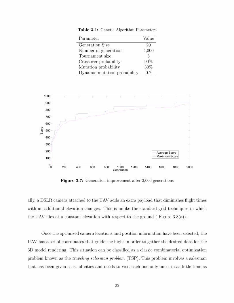
Table 3.1: Genetic Algorithm Parameters
Parameter Value
Generation Size 20Number of generations 4,000Tournament size 3Crossover probability 90%Mutation probability 30%Dynamic mutation probability 0.2
0 200 400 600 800 1000 1200 1400 1600 1800 20000
100
200
300
400
500
600
700
800
900
1000
Generation
Scor
e
Average ScoreMaximum Score
Figure 3.7: Generation improvement after 2,000 generations
ally, a DSLR camera attached to the UAV adds an extra payload that diminishes flight times
with an additional elevation changes. This is unlike the standard grid techniques in which
the UAV flies at a constant elevation with respect to the ground ( Figure 3.8(a)).
Once the optimized camera locations and position information have been selected, the
UAV has a set of coordinates that guide the flight in order to gather the desired data for the
3D model rendering. This situation can be classified as a classic combinatorial optimization
problem known as the traveling salesman problem (TSP). This problem involves a salesman
that has been given a list of cities and needs to visit each one only once, in as little time as
22
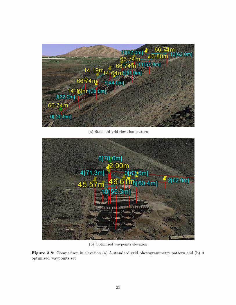
(a) Standard grid elevation pattern
(b) Optimized waypoints elevation
Figure 3.8: Comparison in elevation (a) A standard grid photogrammetry pattern and (b) Aoptimized waypoints set
23

possible. TSP has been widely studied for over 30 years [30], and different methods can be
applied to efficiently to solve this problem.
Unlike on-board path planning for time constraint reasons, which usually relies on
a suboptimal search such as a graph search, the offline optimal path planning uses time-
consuming genetic algorithms that are computed before implementation. This same ap-
proach is used to optimize the camera locations and orientation when solving a TSP type
of problem. A genetic algorithm is applied in such a manner so that each waypoint (city) is
used as the node to be visited.
Previous applications [33] of genetic algorithms to the study of UAVs show that these
algorithms are a flexible optimization method because they can be applied to optimization
problems without continuous first or second derivatives. On the contrary, such algorithms
naturally handle multiple objectives and can incorporate mixed-integer solutions. Genetic
algorithms combine an exploration of the best solution with the new solutions presented by
mutation probability. This is a combination of stochastic and directed search [32].
A measurement of every possibility of a given city for n cities would require n! evalu-
ations. In the case of the 80 waypoints, 80! is 7.1569× 10118 possibilities. Nevertheless, the
use of genetic algorithms decreases this time by evaluating only a small fraction of the total
possible routes. The first step is measuring the distance between all the nodes. Two nodes,
with each node being composed of two cities, are selected at points (x, y) and (a, b), followed
by an attempt to connect these four cities in a different way with a shorter distance. This
measurement can be represented with Equations 3.4a and 3.4b. Where Dij is the distance
from point i to point j. In this case, the four cities are a,b,x and y.
Dxy + Dab < Dxa + Dyb (3.4a)
Dxy + Dab < Dxb + Dya (3.4b)
24

After measuring all distances between each of the cities, the shortest two are selected
as the parents, and then two offspring (tours) are created. If the distance of the new proposed
configuration is shorter than the any of the previous configurations, the same step is repeated
until the shortest global distance is optimal (see Figure 3.9). In order to avoid local minima,
the system introduces diversity in the initial population by using genetic operators such
crossover and mutation.
4.2695 4.27 4.2705 4.271
x 105
4.4239 4.4239 4.4239 4.4239 4.424 4.424 4.424 4.424 4.424
x 106
1405
1410
1415
1420
1425
1430
1435
1440
1445Total Distance = 997.8914, Generation = 42,101
Figure 3.9: Real simulation of a optimized flight path after 42,101 generations
Several [59] combinations of these operators have been devised, and a best set is found
with a mutation procedure. This mutation procedure involves flipping, swapping, and slid-
ing. In this case, the best tournament size is determined to be two. This algorithm provides
suitable solutions for this specific TSP problem and can be adapted to other similar problems.
These functional characteristics of genetic algorithms allows flexibility when finding
the solution to multi-objective problems. Including computer vision principles into the fitness
function optimizes area coverage, and shows an efficient and unique approach for improving
current solutions for photogrammetry problems where detail information is required. This
25

novel design is named Virtual Optimizer for Aerial Routes (VOAR) and is a technique for
optimizing both the flight path and the camera network design.
26

Chapter 4
Laboratory Validation
4.1 Iterative Closest Point and Ray Tracing Algorithm
Ray tracing is a technique that helps to create an image by estimating the positions
[60] that intersect a beam of light that is generated in each of the cameras with a specific
field of view and the distance from the object. Using ray tracing allows computation of
position, orientation and size of objects. Some advanced algorithms also compute reflection,
refraction or dispersion.
Figure 4.1 shows the process in which an object in the far plane is positioned and a
source of light is generated by the algorithm. A camera sends out beams of light that hit
the object and are traced through the scene. The material properties are used to compute
the color of a specific pixel of the object.
Iterative Closest Point [61] (ICP) is selected to assess the quality of a 3D point cloud.
ICP is an algorithm that aligns a partially overlapping set of 3D point clouds by fitting the
data to the points in a reference model. This is done by minimizing the sum of square errors
with the closest model points and data points. The results are presented as a 95% confidence
interval. Figure 4.2 shows the coordinates of a selected point cloud to be compared with a
second point cloud in a ICP test.
4.2 Methodology
A preliminary experiment was selected to test the functionality of the optimization
in which a cube is placed in the center of a bounding box. The image of the cube is rendered
using the ray tracing approach of Chumerin [62]. In the chosen problem formulation a
27

Figure 4.1: Diagram of the ray tracing technique
candidate solution is defined as a set of cameras with corresponding positions and angles
looking towards the center of the scene where the cube is located. To locate the globally
optimal solution, a genetic algorithm is used to lead the search through the fitness function.
The fitness function is defined as the fraction of rays hitting the face of the cube
relative to the total surface. The fitness function of the potential solution is evaluated and
used to generate a new set of solutions through crossover and mutation operators. Crossover
is the main operator that improves the current solution by the exchange of genetic material
between solutions. This operation occurs as often as a given probability. To converge faster
to the global optimal solution, the selected probability is set at 80%. See Appendix A for
the complete source code.
A laboratory test is devised to test the algorithm and evaluate the resulting resolution
of a 3D model. The resulting optimal capture locations are used to guide placement of a
camera in a real cardboard quadrant (1m× 1m× 1m) with an internal grid of 5 cm.
28

Figure 4.2: Iterative closest point measurements
There are cubes of different sizes(5, 10, 15 and 20 cm) placed successively at the
center of the quadrant. A cube of 20 cm is shown in Figure 4.3.
4.3 Results
The optimization algorithm is performed using 18 and 24 camera locations, with 3
types of cameras, a Nikon D7100 DSLR with 35 mm lens, a Panasonic Lumix ZS30 with a
24 mm lens and a GoPro Hero 3 black edition with a 5.4 mm flat lens. After the optimiza-
tion and the image capture the images are processed using CMPMVS, an open source SfM
algorithm[26] (See Figure 4.4).
A quality assessment is performed by the Iterative Closest Point (ICP) [61] in Cloud
Compare, an open source program released under the GNU General Public License. The
four vertical sides of the cube are measured with four separate measurements each. The 95%
confidence interval of the distance measurements is computed.
29

(a) Simulated Bounding Box
(b) Real Coordinate System
Figure 4.3: Simulated and Real Bounding Box
30

Results are shown in Table 4.1. Given the nature of the scaled experiment and the
field of view of the sensors used, some models couldn’t be developed or analyzed properly
and are omitted.
Table 4.1: 95% Confidence Interval Quality Assessment Results
Camera 5 10 15 20(Pictures) (cm) (cm) (cm) (cm)
Nikon (24) 5.0085 − 5.1432 9.8117 −10.0742 15.0002− 15.2123 19.6559−19.8679Nikon (18) 5.0539 − 5.1441 9.6818 −10.0458 14.4786− 14.6990 19.6635−19.8602LumiX (18) 4.6382 − 5.0428 − − −GoPro (24) 4.4230 − 4.7730 − − −
These results plotted in Figure 4.5 show the upper and lower limits of the confidence
intervals of the models using 18 and 24 pictures. The number of pictures used to produce
the model did not have a significant impact on the final resolution of the generated point
cloud, the model that includes 24 pictures has similar tolerances to the models created with
only 18 pictures.
4 6 8 10 12 14 16 18 20−1
−0.8
−0.6
−0.4
−0.2
0
0.2
0.4
0.6
0.8
1
Distance (cm)
Con
fiden
ce In
terv
al (c
m)
Measured DistanceNikon 24 PhotosNikon 18 Photos
Figure 4.5: 95% Confidence Interval Accuracy using Nikon DSLR
31

(a) Lateral view of the box in the 3D model
(b) Upside view of the box using 18 pictures with Nikon DSLR
Figure 4.4: 3D models used for the quality assessment
32

There is a point of diminishing returns in which including more pictures doesn’t have
a significant impact in the final outcome. This information is used to determine the number
of pictures required per survey area depending on the desired accuracy.
The ability to take fewer pictures while covering the same amount of area and produce
a model with greater resolution has a great effect on the flight time of the UAV. This allows
for a larger area to be covered in one flight and the ability to produce larger single models.
The optimal number of photos is not calculated in this work. In each case, a fixed number
of photos is arbitrarily selected. This optimization problem is left for future work.
The factor that makes the greatest difference in the resolution of the point cloud
models is the resolution of the sensor. The Nikon D7100 DSLR camera has the highest
resolution of the cameras tested and is capable of producing models for all box sizes because
of the sufficient field of view. The other camera were only capable of producing viable models
with a 5 cm cube. As seen in Table 4.1 the accuracy of these point clouds is much greater
in the models produced by the Nikon sensor for the 5 cm cube and is expected to be higher
for other sizes as well.
33

Chapter 5
Field Trial Validation
5.1 Multi Objective Optimization
This experiment was developed in a remote area of what used to be the Tintic Stan-
dard Reduction Mill near Goshen, Utah, USA, built in 1920 to process metals like copper,
gold and silver. There now remains the ruins of tanks and foundations of cylindrical struc-
tures (see Figure 5.1). The unique building structure and remoteness of the mill offers a
unique location to measure efficiency and accuracy of the algorithm. This field evaluation
site is representative of some structures of interest for 3D modeling and infrastructure mon-
itoring. Chemical plants, refineries, offshore oil platforms, pipeline terminals, dams, bridges
and other structures share similar size and feature characteristics to this particular location.
Figure 5.1: Aerial view of the standard reduction mill
34

The images were acquired by a GoPro Hero 3 Black Edition camera which was carried
by a multi-rotor DJI phantom 2 and mounted in a 2-axis gimbal. The 2-axis gimbal stabilizes
the camera in tilt (pitch) and roll. Even though the algorithm has the capability of working
with the camera with up to 3 degrees of freedom (roll, tilt and pan), for the purposes of
this research the camera was fixed facing down at 90°during the flights. This restriction was
imposed because of the difficulty in synchronizing image capture and multirotor communi-
cation. Future work will address the automation challenge of synchronizing the multi rotor
platform, the automated camera 3 axis gimbal as well as the camera shutter.
Two flight test were conducted at the mill. Each was controlled autonomously via
waypoint control through a 2.4 GHz datalink between the multi-rotor and a laptop. An
evenly spaced set of lines over an area of interest in which images needs to be captured is
commonly known as a grid. A grid planning tool was used to plan the first flight path. The
Virtual Optimizer for Aerial Routes (VOAR) selected locations for the second test flight.
The outcome of the first one resulted in a flight path with 14 waypoints and 80 camera lo-
cations from which the 3D model was reconstructed. The same number of camera locations
were used in the optimization algorithm.
As shown in Figure 5.2. With initial camera locations, the functional coverage is 4%.
The functional coverage of the last configuration after 4,000 generations(see Figure 5.3) is
64%. The diversity of configurations given in the parameters of the genetic algorithm allows
the final network design to spread the waypoints over the terrain maximizing the coverage
while diversity constraints within the fitness function ensure multiple angle views of each
point.
5.2 Qualitative Analysis
After the flights, both set of pictures are processed using CMPMVS and the qualita-
tive results are summarized in Figures 5.4 and 5.5. Because the non optimized grid path is
limited to capture images along the fixed parallel lines inside the selected polygon (Figure
5.4(a)), the final point cloud lacks of sufficient information between these lines, as seen in Fig-
35

4.26884.269
4.26924.2694
4.26964.2698
4.274.2702
4.27044.2706
x 105
4.42334.4233
4.42344.4234
4.42344.4234
4.42344.4235
4.42354.4235
x 106
1380
1400
1420
1440
1460
1480
1500
(a) First generation of camera locations, blue dots represents the 4% functional coverage
4.2694.2692
4.26944.2696
4.26984.27
x 1054.4234
4.4234
4.4234
4.4234
4.4234
4.4235
4.4235
x 106
1400
1410
1420
1430
1440
1450
1460
1470
1480
(b) Last generation of camera locations, blue dots represents the 64% functional coverage
Figure 5.2: First and last generation of the camera location optimization
ure 5.4(b). While having adequate resolution in the covered areas, the lack of information in
the middle decreases the overall quality of the model as further discussed in the next section.
Optimizing the camera locations has the effect of spreading the camera image collec-
tion points to satisfy the fitness function and at the same time maximize the coverage of the
80 camera locations as seen in Figure5.5(a). Not only is the coverage increased partially by
36

0 500 1000 1500 2000 2500 3000 3500 40000
100
200
300
400
500
600
700
800
900
Average Max
Figure 5.3: Generation improvement over the time
the altitude change of every point of the network, but also the quality of the whole model
is improved by the constant overlapping of the images. The resulting model shows an even
better 3D reconstruction of the scene with fairly even resolution as shown in Figure5.5(b).
5.3 Quantitative Analysis
The models are analyzed using the same approach as in the laboratory validation.
For the mill, seven different elements of the factory are selected from different locations. The
ICP analysis is performed and the results are summarized in Table 5.1.
Whereas the standard grid gives a 95% confidence interval between 6 and 8% relative
to the ground truth, the optimized network presented a 2 to 5% difference from ground truth
(See Figure 5.6). This significant difference is attributed to the requirement of the fitness
function of pairwise overlap of 50% and 80% and the priority to designs where camera poses
are in at least 3 of the 5 regions in which the terrain is divided.
There are other factors such the altitude variation (see Figure 5.7). This variation
allows the field of view to increase and to cover more area. This explains that the first model
is strictly of the area of the square grid. The second model includes this same area but the
37

(a) Standard grid planning
(b) 3D model using grid planning
Figure 5.4: Field validation results using standard grid planning
38

(a) VOAR coordinate system
(b) 3D model using VOAR
Figure 5.5: Field validation results using VOAR
39

200 300 400 500 600 700 800 900 1000−100
−50
0
50
100
Distance (cm)
Con
fiden
ce In
terv
al (c
m)
Measured DistanceStandard GridVOAR
Figure 5.6: 95% confidence interval of the field test
Table 5.1: 95% Confidence Interval Quality Assessment Results
Element Ground Truth Standard Grid V OAR(cm) (cm) (cm)
Wall 1 574.54 571.77−619.81 527.31−565.06Wall 2 521.51 530.69−557.01 498.43−534.70Wall 3 216.25 198.42−229.11 228.55−256.41Vessels 888.49 863.04−938.96 885.43−953.73Stem Wall 1 953.26 864.83−971.62 894.56−958.95Stem Wall 2 992.73 892.84−968.64 972.38− 1031.03Stem Wall 3 206.95 191.18−243.29 202.86−223.96
algorithm and the constraints provide better coverage with higher resolution. The coverage
improved 35% in the width and 22% in the length, also there is not blurry or empty sections
in the final model.
40

Figure 5.7: Flight path resulting from the optimization
The average altitude is 15.2 m with a highest altitude of 22 m and a lowest altitude
of 11 m with respect to the ground. The velocity from point to point is fixed at 4 m/s with
4 s of hold time to allow the camera to take the picture. A wind speed of 5-7 mph influenced
the flight time.
One drawback of the altitude variation (see Figure 5.8) for the optimized solution
is that there is a higher battery consumption when compared with a non-optimized grid
pattern. After 100,850 generations of the genetic algorithm the distance is reduced from an
initial guess of 625.9 m to 450.7 m for the optimized flight path. That represents a 28%
decrease from an initial guess.
The standard grid design (non-optimized) flight path has 9.5 minutes of flight time
compared to 17 minutes for the optimized camera location flight path. Future work will
address the coupling and trade off between camera location diversity and other factors such
as minimized flight time.
41

Figure 5.8: View of the DJI groundstation for 15 of the optimized waypoints
42
Chapter 6
Optimization Under Different Scenarios
6.1 Privacy Assurance
Because UAV surveillance cameras are mobile and airborne, anything that is above
ground is potentially under surveillance from the UAV sensor. However, many citizens,
companies, organizations, and government agencies have expressed a strong desire to avoid
surveillance by an airborne sensors such as a UAV surveillance camera [63]. On the other
hand, the forecast of productive and non-invasive economic activity related to commercial
UAV is significant.
Privacy assurance is needed in parallel with the development of infrastructure moni-
toring. When performing remote sensing there may be regions of the terrain that are more
important to observe than others, along with private areas that should not be observed. The
objective of privacy assurance is to view regions of interest while avoiding observation of
private areas.
Privacy assurance is enabled by creating a reward and penalty map, adapted from
the previous work of Niedfeldt et al. [49]. The reward map displays potential desirible areas
available to the system if it observes the terrain point z. The reward map is denoted as r(t,
z, x), which indicates the available reward at the terrain point z at time t. The reward map
is updated using sensor measurements according to the current state vector x with a two
dimensional Gaussian distribution centered on the nearest point in the region of interest to
the terrain point z.
43

Figure 6.1: Representation of a reward and penalty map
6.2 Planning and Simulation
The purpose of the privacy protection path planner is to reduce the effort needed to
prepare for and fly a surveillance mission near private areas by autonomously computing
both a flight path and a sensor schedule. The planning algorithm is implemented with a set
of z discrete terrain points defining the region of interest obtained from the US Geological
Survey online database.
For the purposes of this study, a fixed camera is used in the path planner, pointing
directly downward relative to the aircraft body. Because a multi-rotor platform is used,
the sensor path is planned first, and the UAV path is defined using the same latitude and
longitude coordinates at a fixed elevation above the sensor path.
In order to evaluate the privacy protection planner, a performance metric is defined.
The private areas are divided into 5 × 5 meter sectors, and the center point of each sec-
tor is calculated. The total number of privacy sectors is recorded. The flight path is then
simulated, and it is determined how many privacy sectors are violated over the course of
the flight, based on the number of sector center points seen. The privacy areas defined
44

for the flight tests are shown in Figure 6.2. The desired region of observation is shown in
green. The private areas are marked in white. The planned flight path is shown in Figure 6.3.
Figure 6.2: Test area and privacy areas
6.3 Flight Test
The goal of the flight demonstration is to fly the planned path shown in Figure 6.3
and compare the predicted privacy violation to what is actually observed. A DJI Phantom
quadcopter was selected since it is a widely used consumer platform, and a GoPro Hero3
Black Edition color camera. Video is captured in 1920 × 1080 resolution at 50 frames per
second. The camera is set to use the narrow field of view (FOV) setting and mounted to
point below the body of the UAS, as shown in Figure 6.4 The DJI Groundstation software
is used to control the UAS during the flight.
45

Figure 6.3: Planned flight path
To asses the performance of the simulator in actual flight tests, the center points of
the test area privacy sectors are marked using brightly colored marking cones located using
GPS coordinates. The flights are performed, and the resulting video are closely examined
to determine the number of cones seen throughout the flight. Two flights were performed
using the same flight path. Figure 6.5 shows the locations of the marking cones. The results
of the simulation are compared with the results of the flight tests in Table 6.1.
Table 6.1: Privacy Protection Results
Test Penalty Sectors Violated
Simulated 11Flight one 2Flight two 4
46

Figure 6.4: DJI phantom quadcopter used for this study
Figure 6.5: Simulation of the aerial view of the private sectors
The increase in penalty areas violated during the second flight as compared to the first
flight is due to an increase in wind. This made it more difficult for the autopilot to control
the flight, and led to increased deviations from the ideal straight down camera direction.
However, both flights produced satisfactory results. Surprisingly, the simulation predicted
that a higher number of privacy sectors would be violated than were actually violated during
the test flights.
47

Figure 6.6: Actual flight path
Possible explanations may include a failure to completely capture the camera pa-
rameters and settings in simulation, and inaccuracy in the GPS positioning of the marking
cones.
48

Chapter 7
Conclusion and Future Considerations
Numerous use cases are developed for the application of UAV-based remote sensing.
Each of these use cases involves different implications for the capabilities needed on-board the
UAV. For test purposes a commercial sensor is used. However each case study is basis for the
development of the concept of remote sensing, including DSLR, thermal, or infrared cameras.
Genetic algorithms solve a camera positioning problem with multiple objectives. As
part of this study, a genetic algorithm is developed and tested to maximize the image cov-
erage of 80 cameras across the remains of an abandoned factory in Goshen, Utah. After
4,000 generations, the functional coverage required for SfM increased from 2% to 64%. The
optimized flight path of the UAV for capturing these images is further optimized by using the
Traveling Salesman Problem approach, reducing the flight distance by 28% from the initial
estimation. However, the optimized solution does sacrifice efficiency in data collection rela-
tive to a standard grid pattern that is commonly used in photogrammetric autopilot software.
This new algorithm optimizes flight paths to monitor infrastructure using GPS co-
ordinates and optimized camera positions ensuring maximized information content of the
captured images. As a result, the images provide detailed information from places where
human or manned aircraft access may be difficult. Combining optimization techniques, au-
tonomous aircraft, and computer vision methods presents a novel approach for infrastructure
monitoring. Specific contributions involved in this work can be summarized as:
� Development of an optimized camera network
49

� Optimization of camera orientation
� Flight path planning to visit optimized camera network locations
The final output of a three-dimensional digital model from civil and chemical infras-
tructure is of great interest, especially in fields where routine maintenance is needed. This
study demonstrates the advantages of aerial photogrammetry. The quality of the laboratory
results demonstrate sub centimeter (≤ ±1 cm compared to the ground truth) resolution can
be reached .
These results show that there is a promising field in applying optimization techniques
to improve the performance and efficiency of high resolution UAV monitoring. Optimization
techniques build upon aerospace and computer science innovations to increase the effective-
ness of UAV technologies in a wide variety of applications.
Pipelines and power lines are currently inspected by manned aircrafts to detect po-
tential leakage. These inspections are generally conducted by a small aircraft or helicopter
with a pilot and an additional observer or sensor operator. Using UAVs to perform remote
sensing can significantly reduce the cost of the operation and will allow operators to perform
inspections more frequently for pipeline monitoring, power line inspection, or civil infras-
tructure assessment. As with search and rescue operations, the lower altitudes and slower
speeds provide benefits for infrastructure inspections as well.
Some inspections may involve UAV flights and the collection of image data in less pop-
ulated areas. Nevertheless, other inspections may be in close proximity to areas that present
privacy and safety issues. It is important to ensure that a UAV is not used to perform inap-
propriate surveillance of a privacy zone near the area of interest during a required inspection.
Future work should consider the use of an inertial measurement unit (IMU) for mea-
suring velocity, orientation, and gravitational forces or Real Time Kinematic GPS coupled
to the sensor for improved geotagging and faster computer processing. Having five degrees of
50

freedom in the gimbal will allow greater diversity of location with respect to where pictures
can be taken. Furthermore, the use of reward and penalty maps in the development of the
flight paths will be beneficial for monitoring civil and chemical infrastructures and avoiding
privacy issues.
In conclusion, UAV-based platforms can be used for regular, programmed inspections
by creating 3D models that provide detailed analysis. The use of these tools will undoubtedly
lead to a greater preventive approach to monitoring and managing infrastructure.
51

Appendix
Appendix A Genetic Algorithm Source Code
This script finds the optimal camera positions and the optimal flight path for SFM
reconstruction of a 3D scene using raytracing and a genetic optimization algorithm.
clear all
close all
clc
warning(’off’,’all’)
warning
global childBest
%set(gcf, ’NumberTitle’, ’off’)
tic
% Parameters
%Algorithm
generationSize = 20
numberOfGenerations = 40
tournamentSize = 4
crossoverProbability = .9
mutationProbability = .3
dynamicMutationParameter = .2
numberOfCameras = 75
52

%Load terrain
disp(’Loading Terrain’)
mapName = ’azu1’terrain, Xmin, Xmax, Ymin, Ymax, Zmin, Zmax, terrainHeight, terrainWidth, mapZone
= loadTerrain(mapName)
%Camera Parameters
disp(’Initializing Camera’)
focalLength = .014
imageWidth = 4000
imageHeight = 3000
nearPlane = 2
farPlane = 45
viewingAngle = 5*pi/180
camera.focal length0 = focalLength
camera.dmin = nearPlane
camera.dmax = farPlane
camera.alpha = viewingAngle*imageHeight/imageWidth
camera.beta = viewingAngle
camera.resX = imageWidth
% pixels camera.resY = imageHeight
% pixels camera.focal length = focalLength
camera.fovVert = getFovVert(camera.alpha, camera.beta, camera.dmin, camera.dmax)
%Bounding box xmin = Xmin-45
xmax = Xmax+45
ymin = Ymin-45
ymax = Ymax+45
zmin = Zmax
53

zmax = Zmax+45
%Camera rotation range
phiMin = 0
% phiMax = 359
phiMax = 0
% uncomment this if using phanthom looking down
% thetaMin = -180
thetaMin = -90
% uncomment this if using phanthom looking down
thetaMax=-90
% Initialize genetic algorithm
parent = newPopulation(generationSize,numberOfCameras,xmax,ymax,zmax,xmin,
ymin,zmin,phiMin,phiMax,thetaMin,thetaMax)
% scoring parameters
parentCandidateScores(:,1) = linspace(1,generationSize,generationSize)
childCandidateScores(:,1) = linspace(1,generationSize,generationSize)
% Optimization
for n = 1:numberOfGenerations
n
if n == 1
%Score Parent
for c = 1:generationSize
candidateScore = 0
54

candidate = parent(parent(:,4)==c,:)
candidateScore = scoreCandidate( candidate, terrain, numberOfCameras,
terrainHeight, terrainWidth, camera, mapZone)
parentCandidateScores(c,2) = candidateScore
end firstGenerationAverage = mean(parentCandidateScores(:,2))
firstGenerationMax = max(parentCandidateScores(:,2))
generationScores(1,1) = 0
generationScores(1,2) = firstGenerationAverage
generationScores(1,3) = firstGenerationMax
firstBestNumber = parentCandidateScores(parentCandidateScores(:,2)==firstGenerationMax,1)
firstBest = parent(parent(:,4)==firstBestNumber(1),:)
end
%Create Child
p = 1
while p ¡= generationSize candidateNumber = p
%Tournament [mother father] = tournament(parentCandidateScores,tournamentSize,generationSize)
%Crossover
r = randi(10,1)/10
if r < crossoverProbability
[childA childB] = crossover( mother, father, parent, numberOfCameras, candidateNumber)
else
childA = parent(parent(:,4)==mother,:)
childA(:,4) = candidateNumber
childB = parent(parent(:,4)==father,:)
childB(:,4) = candidateNumber+1
end
%Mutation
55

childA = mutate(childA,dynamicMutationParameter,mutationProbability,
numberOfCameras,n,numberOfGenerations,xmin,xmax,ymin,ymax,zmin,zmax,
phiMin,phiMax,thetaMin,thetaMax)
childB = mutate(childB,dynamicMutationParameter,mutationProbability,
numberOfCameras,n,numberOfGenerations,xmin,xmax,ymin,ymax,zmin,zmax,
phiMin,phiMax,thetaMin,thetaMax)
%Append to child
if p == 1
child = childA
child = vertcat(child,childB)
else child = vertcat(child,childA)
child = vertcat(child,childB)
end p = p + 2
end
%Score Child for c = 1:generationSize candidateScore = 0
candidate = child(child(:,4)==c,:)
candidateScore = scoreCandidate( candidate, terrain, numberOfCameras,
terrainHeight, terrainWidth, camera, mapZone)
childCandidateScores(c,2) = candidateScore
end childCandidateScores(:,1) = linspace(1,generationSize,generationSize)
%Elitism childCandidateScores(:,1) = childCandidateScores(:,1) + generationSize
combinedPopulationScores = vertcat(parentCandidateScores,childCandidateScores)
combinedPopulationScores = sortrows(combinedPopulationScores,-2)
childCandidateScores = combinedPopulationScores(1:generationSize,:)
child(:,4) = child(:,4) + generationSize
56
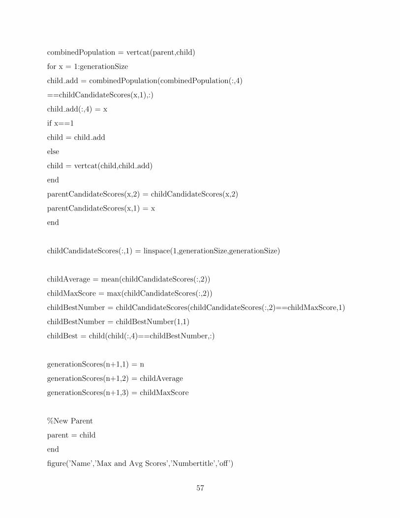
combinedPopulation = vertcat(parent,child)
for x = 1:generationSize
child add = combinedPopulation(combinedPopulation(:,4)
==childCandidateScores(x,1),:)
child add(:,4) = x
if x==1
child = child add
else
child = vertcat(child,child add)
end
parentCandidateScores(x,2) = childCandidateScores(x,2)
parentCandidateScores(x,1) = x
end
childCandidateScores(:,1) = linspace(1,generationSize,generationSize)
childAverage = mean(childCandidateScores(:,2))
childMaxScore = max(childCandidateScores(:,2))
childBestNumber = childCandidateScores(childCandidateScores(:,2)==childMaxScore,1)
childBestNumber = childBestNumber(1,1)
childBest = child(child(:,4)==childBestNumber,:)
generationScores(n+1,1) = n
generationScores(n+1,2) = childAverage
generationScores(n+1,3) = childMaxScore
%New Parent
parent = child
end
figure(’Name’,’Max and Avg Scores’,’Numbertitle’,’off’)
57
plot(generationScores(:,1),generationScores(:,2))
hold on
plot(generationScores(:,1),generationScores(:,3),’m’)
legend(’Average’,’ Max’,’Location’,’southeast’)
% figure
% scatter3(childBest(:,1),childBest(:,2),childBest(:,3),’r’)
% hold on
% scatter3(firstBest(:,1),firstBest(:,2),firstBest(:,3))
% hold on
%Plot First and Last
plotCandidate(firstBest, terrain, numberOfCameras, terrainHeight, terrainWidth, camera,
mapZone)
% title(’First Generation Max’)
plotCandidate(childBest, terrain, numberOfCameras, terrainHeight, terrainWidth, camera,
mapZone)
%break %title(’Last Generation Max’)
%Final Scores
[score1, coverage1, functionalCoverage1] = scoreCandidate(firstBest, terrain,
numberOfCameras, terrainHeight, terrainWidth, camera, mapZone)
[score2, coverage2, functionalCoverage2]= scoreCandidate(childBest, terrain,
numberOfCameras, terrainHeight, terrainWidth, camera, mapZone)
%Plot Terrain
% x = reshape(terrain(:,:,2),1,[ ])
% y = reshape(terrain(:,:,1),1,[ ])
% z = reshape(terrain(:,:,3),1,[ ])
58
% scatter3(x,y,z,’b’)
%plotcube([100 100 100],[-50 -50 -50],.8,[1 0 0])
%hold on
axis equal
% resize matrix
% %
%————–> Next Stage
% utmzone=12
% childBest(:,6)=[ ]
% childBest(:,5)=[ ]
% childBest(:,4)=[ ]
% childBest(:,3)=[utmzone]
% utmzone=12
% xx=childBest(:,1)
% yy=childBest(:,2)
% % [Lat,Lon] = utm2deg(xx,yy,utmzone)
%initialize path planner
%break
disp(’initializing Optimizer ...’)
pause(3)
VOAR()
% toc
<————– End main script
59

SCRIP FOR THE FUNCTION “LOAD TERRAIN”
function [terrain,Xmin,Xmax, Y min, Y max, Zmin, Zmax, imageHeight, imageWidth,mapZone]
= loadTerrain( mapName )
%loadTerrain: Given map name, loads terrain points from kml file
format long
% mapName=(’azu1’)
%Import kml file named mapName.kml from /maps/mapName/
filePath = strcat(’maps/’,mapName,’/’,mapName,’.kml’)
struct = kml2struct(filePath)
%%Extract reward area, penalty area, and launch point from struct
numberReward = nnz(strcmp(struct.Name,mapName))
rewardElements = find(strcmp(struct.Name,mapName))
for i = 1:numberReward
rewardPolygonLon(1:numel(struct(rewardElements(i)).Lon),i) =
struct(rewardElements(i)).Lon
rewardPolygonLat(1:numel(struct(rewardElements(i)).Lat),i) =
struct(rewardElements(i)).Lat
end
%Remove NaN from loop
rewardPolygonLon(isnan(rewardPolygonLon))=0
rewardPolygonLat(isnan(rewardPolygonLat))=0
%Calculate Map Limits
maxLat = max(rewardPolygonLat(rewardPolygonLat =0))
60

minLat = min(rewardPolygonLat(rewardPolygonLat =0))
maxLon = max(rewardPolygonLon(rewardPolygonLon =0))
minLon = min(rewardPolygonLon(rewardPolygonLon =0))
%Convert limits to UTM for image sizing - 5m sections
[x min, y min,mapZone] = deg2utm(minLat,minLon)
[x max, y max] = deg2utm(maxLat,maxLon)
imageHeight = round((y max-y min)/3)
imageWidth = round((x max-x min)/3)
Xmin = round(x min)
Xmax = round(x max)
Ymin = round(y min)
Ymax = round(y max)
%%Get Map
ortho = wmsfind(’SDDS Imagery’, ’SearchField’, ’serverurl’)
% ortho = wmsfind(’elevation’, ’SearchField’, ’serverurl’)
ortho = refine(ortho, ’Orthoimagery’, ...
’SearchField’, ’serverurl’)
layers = wmsfind(’nasa.network’, ’SearchField’, ’serverurl’)
% layers = wmsfind( ’elevation’)
us ned = layers.refine(’usgs ned 10’)
% us ned = layers.refine(’SRTM3-World’)
latlim = [minLat maxLat]
lonlim = [minLon maxLon]
% A = wmsread(ortho, ’Latlim’, latlim, ’Lonlim’, lonlim, ...
% ’ImageHeight’, imageHeight*5, ’ImageWidth’, imageWidth*5)
61

[Z,R] = wmsread(us ned, ’ImageFormat’, ’image/bil’, ...
’Latlim’, latlim, ’Lonlim’, lonlim, ...
’ImageHeight’, imageHeight, ’ImageWidth’, imageWidth)
[latlon] = findm(Z,R)
[XY ] = deg2utm(lat, lon)
Y = reshape(Y,imageHeight,imageWidth)
X = reshape(X,imageHeight,imageWidth)
Zmin = min(Z(:))
Zmax = max(Z(:))
terrain(:,:,1) = Y
terrain(:,:,2) = X
terrain(:,:,3) = Z
% %Render Map Image (Optional)
% figure(’Renderer’,’opengl’)
% usamap(latlim, lonlim)
% axesm utm
% zone = utmzone([minLat minLon])
% setm(gca,’mapprojection’,’utm’,’zone’,zone,’maplatlimit’,latlim,’maplonlimit’,lonlim)
% framem off
mlabel off
plabel off
gridm off
% geoshow(double(Z), R, ’DisplayType’, ’surface’, ’CData’, A)
% daspectm(’m’,1)
% title(mapName, ...
62

% ’FontSize’,8)
% axis vis3d
%Graph Terrain Points
x = reshape(X,1,[ ])
y = reshape(Y,1,[ ])
z = reshape(Z,1,[ ])
%scatter3(x,y,z)
end
<—————————– End fucntion “load terrain”
63

SCRIPT FOR THE FUNCTION “CROSSOVER”
function [ childAchildB] = crossover( mother, father, parent,
numberOfCameras, candidateNumber)
%Crossover: Mixes two parent candidates to create two children using Blend
%crossover.
motherCandidate = parent(parent(:,4)==mother,:)
fatherCandidate = parent(parent(:,4)==father,:)
for i=1:numberOfCameras
r = randi(10,1)/10
for j=1:3
childA(i,j) = r*motherCandidate(i,j) + (1-r)*fatherCandidate(i,j)
childB(i,j) = (1-r)*motherCandidate(i,j) + r*fatherCandidate(i,j)
end
for j=5:6
childA(i,j) = r*motherCandidate(i,j) + (1-r)*fatherCandidate(i,j)
childB(i,j) = (1-r)*motherCandidate(i,j) + r*fatherCandidate(i,j)
end
childA(i,4) = candidateNumber
childB(i,4) = candidateNumber+1
end
end
64

SCRIPT FOR FUNCTION “MUTATE”
function candidate = mutate( candidate, mutationParameter, mutationProbability,
numberOfCameras, generation, numberOfGenerations, xmin, xmax, ymin, ymax, zmin,
zmax,phiMin,phiMax,thetaMin,thetaMax)
%Introduces diversity by randomly changing child genes.
%Utilizes dynamic mutation parameter beta to decrease mutation as
%generations go on.
a = (1-(generation-1)/numberOfGenerations) ˆ mutationParameter
zmin = double(zmin)
zmax = double(zmax)
for i=1:numberOfCameras
r = randi([110 ],1)/10
if r < mutationProbability
%Mutate x
rx = randi([xminxmax ],1)
x = candidate(i,1)
if rx <= x
candidate(i,1) = xmin + (rx-xmin) ˆ a *(x-xmin)(1-a)
else
candidate(i,1) = xmax - (xmax-rx) ˆ a*(xmax-x) ˆ (1-a)
end
%Mutate y
ry = randi([yminymax ],1)
y = candidate(i,2)
if ry <= y
65

candidate(i,2) = ymin + (ry-ymin) ˆ a*(y-ymin) ˆ (1-a)
else
candidate(i,2) = ymax - (ymax-ry) ˆ a*(ymax-y) ˆ (1-a)
end
%Mutate z
rz = randi([zminzmax ],1)
z = candidate(i,3)
if rz <= z
candidate(i,3) = zmin + (rz-zmin) ˆ a*(z-zmin) ˆ (1-a)
else
candidate(i,3) = zmax - (zmax-rz) ˆ a*(zmax-z) ˆ (1-a)
end
%Mutate phi
rp = randi([phiMinphiMax ],1)
p = candidate(i,5)
if rp ¡= p
candidate(i,5) = phiMin + (rp-phiMin) ˆ a*(p-phiMin) ˆ (1-a)
else
candidate(i,5) = phiMax - (phiMax-rp) ˆ a*(phiMax-p) ˆ (1-a) end
%Mutate theta
rt = randi([thetaMinthetaMax ],1)
t = candidate(i,6)
if rt <= t
candidate(i,6) = thetaMin + (rt-thetaMin) ˆ a*(t-thetaMin) ˆ (1-a)
else
candidate(i,6) = thetaMax - (thetaMax-rt) ˆ a*(thetaMax-t) ˆ (1-a)
end end end end
66

SCRIP FOR THE FUNCTION “SCORE CANDIDATE”
function [ score, coverage, functionalCoverage] =
scoreCandidate( candidate, terrain, numberOfCameras, terrainHeight,
terrainWidth, camera, mapZone)
%candidateScore returns a score for a set of cameras.
%Min and Max indices
areaIndices(1,1) = 1
areaIndices(1,2) = 1
areaIndices(2,1) = terrainHeight
areaIndices(2,2) = terrainWidth
%Terrain Center
x center = mean(mean(terrain(:,:,2)))
y center = mean(mean(terrain(:,:,1)))
z center = mean(mean(terrain(:,:,3)))
allIndexes = [ ]
numVisiblePoints = 0
visibilityMatrix = zeros(numel(terrain(:,:,1)),numberOfCameras)
%Which cameras can see which points
for j=1:numberOfCameras
camera position = [ candidate(j, 1)candidate(j, 2)candidate(j, 3)]
zone = mapZone
67

[ cameraLat, cameraLon] = utm2deg(candidate(j,1),candidate(j,2),zone)
[ centerLat, centerLon] = utm2deg(x center,y center,zone)
%plotCamera( terrain,candidate(j,1),candidate(j,2),candidate(j,3),x center,y center,z center)
%Frustum Cull visibility = frustumCull fast3(terrain,candidate(j,1),candidate(j,2),candidate(j,3),
candidate(j,5), candidate(j,6),0)
%[ pointsInFrustrum pointsInFrustrum grid] = frustumCull new(candidate(j,
2), candidate(j,1), -candidate(j,3), 0, 0, 0, terrain, camera, areaIndices)
%Points in Frustum
indexes = find(visibility == 1)
x = reshape(terrain(:,:,2),1,[ ])
y = reshape(terrain(:,:,1),1,[ ])
z = reshape(terrain(:,:,3),1,[ ])
x sub = x(indexes)
y sub = y(indexes)
z sub = z(indexes)
%Plot Seen Points %scatter3(x sub,y sub,z sub,’filled’)
if(numel(indexes>2))
%Hidden Point Removal
p = [ x sub′ y sub′ z sub′]
r = 90
try
visiblePtInds = HPR(p,camera position,r)
indexes = indexes(visiblePtInds)
catch
%disp(’Strange Error’)
68

indexes = indexes
end
%indexes = indexes(visiblePtInds)
visibilityMatrix(indexes,j) = 1
else
visibilityMatrix(indexes,j) = 1
end
allIndexes = vertcat(allIndexes,indexes)
numVisiblePoints = numel(unique(allIndexes))
%score = numVisiblePoints
end
%Score each point
pointScores = zeros(numel(x),1)
distanceLimit = 45
covered = 0
coveredFunctional = 0
for i=1:numel(x)
camInd = find(visibilityMatrix(i,:)>0)
if(numel(camInd)>0)
%Cameras that see each point
camerasThatSeePoint = numel(camInd)
%Coverage Calc
covered = covered + 1
if(numel(camInd)>2)
69

coveredFunctional = coveredFunctional + 1
%Angle they see them from
numX = numel(candidate(camInd,1))
Zones = {}
for j=1:numX
Zones{j,1} = zone
end camerasLat = [ ]
camerasLon = [ ]
for j=1:numX
[ camLat, camLon] = utm2deg(candidate
(camInd(j),1),candidate(camInd(j),2),Zones{j,1})
camerasLat = vertcat(camerasLat, camLat)
camerasLon = vertcat(camerasLon, camLon)
end
[ pointLat, pointLon] = utm2deg(x(i),y(i),zone)
[ angle, range, az] =
elevation(pointLat,pointLon,z(i),camerasLat,camerasLon,candidate(camInd,3))
%Cameras in each third of the hemisphere
tri1 = az(az > 0 az <= 120)
tri1 = numel(tri1)
if(tri1>0)
tri1=1
end
tri2 = az(az > 120 az <= 240)
tri2 = numel(tri2)
if(tri2>0)
tri2=1
70
end
tri3 = az(az > 240 az < 360)
tri3 = numel(tri3)
if(tri3>0)
tri3=1
end
%Max camera distance
maxCamDist = max(range)
%Score for this point
%pointScores(i) = (camerasThatSeePoint - 2) - (maxCamDist/distanceLimit)
+ (tri1+tri2+tri3)
%distMult = min([ (maxCamDist/distanceLimit)1])
pointScores(i) = ((camerasThatSeePoint - 2) + (tri1+tri2+tri3))
end
end
%Sum point scores
score = sum(pointScores)
%Coverage
coverage = covered/numel(x)
functionalCoverage = coveredFunctional/numel(x)
end
71

SCRIPT FOR FUNCTION “VOAR”
% VOAR (Virtual Optimizer for Aerial Routes) takes all the points in which % pictures need
to be taken and plans the shortest path just as the % TSP using a GA.
%coor=coordenates to be visited
%cdis= distances between cordinates
%psize= population size
%gen= generations
%cstate= current state
%res= Result
function varargout = VOAR(coor,cdis,psize,gen,cstate,res)
global childBest r yr
%close all
outs = 6
% Coordenates and Initialize Defaults
yr= childBest
disp(’Finding shortest way ...’)
for s = nargin:outs-1
switch s
case 0
coor = yr
case 1
N = size(coor,1)
a = meshgrid(1:N)
cdis = reshape(sqrt(sum((coor(a,:)-coor(a’,:)).ˆ 2,2)),N,N)
case 2
psize = 20
72

case 3
gen = 1e9 case 4
cstate = 1
case 5
res = 1
otherwise
end
end
% Check up
gen = max(1,round(real(gen(1))))
cstate = logical(cstate(1))
res = logical(res(1))
% Initialize the Population
n = N
pop = zeros(psize,n)
pop(1,:) = (1:n)
for s = 1:psize
pop(s,:) = randperm(n)
end
% Starting the algorithm
gmin = Inf
Tdist = zeros(1,psize)
olddistance = zeros(1,gen)
oldPop = zeros(4,n)
newPop = zeros(psize,n)
if cstate pfig = figure(’Name’,’VOAR — Current State’,’Numbertitle’,’off’)
73

end
% Computing distance
for it = 1:gen
for p = 1:psize
dis = cdis(pop(p,n),pop(p,1))
for s = 2:n
dis = dis + cdis(pop(p,s-1),pop(p,s))
end
Tdist(p) = dis
end
% Shortest distance of the generation
[ mindist, index] = min(Tdist)
olddistance(it) = mindist
if mindist < gmin
gmin = mindist
optimalRoute = pop(index,:)
% Plot the Best Route
figure(pfig)
rte = optimalRoute([ 1 : n1])
% Plot the current state
plot3(coor(rte,1),coor(rte,2),coor(rte,3),’b’, ’LineWidth’,1)
grid on
% grid minor
title(sprintf(’Total Distance = %1.4f, Generation = %d’,mindist,it))
end
74

% GAO randomOrder = randperm(psize)
for p = 4:4:psize % with tournament size 4
rtes = pop(randomOrder(p-3:p),:)
dists = Tdist(randomOrder(p-3:p))
[ ignore, idx] = min(dists)
%ok
bestOf4Route = rtes(idx,:)
routeInsertionPoints = sort(ceil(n*rand(1,2)))
I = routeInsertionPoints(1)
J = routeInsertionPoints(2)
% Mutate the Best to get 3 New Routes for s = 1:4 oldPop(s,:) = bestOf4Route
switch s case 2 % Flip oldPop(s,I:J) = oldPop(s,J:-1:I)
case 3 % Swap oldPop(s,[ IJ ]) = oldPop(s,[ JI])
case 4 % Slide oldPop(s,I:J) = oldPop(s,[ I + 1 : JI])
otherwise % Do Nothing
end
end
newPop(p-3:p,:) = oldPop
end
pop = newPop
end
% Final Plot
disp(’Shortest path found, Preparing final report, please wait...’)
pause(2)
figure(’Name’,’Final Result — Optimum Route’,’Numbertitle’,’off’)
75

plot3(coor(rte,1),coor(rte,2),coor(rte,3),’r.-’)
title(sprintf(’Total Distance = %1.4f, Generation = %d’,mindist,it))
% disp(’The best way to cover this area is visiting in this order:’)
r=rte
Shortestdistance= mindist
%return
disp(’Preparing autopilot file for ground station’)
woodpecker()
disp(’Dividing in batches of 15 waypoints’)
pause( 3 )
disp(’writing mission files...’)
Tesla()
pause( 3 )
disp(’Time consumed to plan the optimal route:’)
t=vpa(tic,6)
disp(’Process completed!’)
tic
76
SCRIPT FOR FUNCTION “ WOODPECKER”
% woodpecker writes the coordinates of the points to be visited before
% and after the optimization, the first are found in the sheet called
% ”points” and the last as ” Opt. Order”, you can also get the information
% of Tilt(Pitch),Roll and Pan (yaw)for the camera
syms x1 x2 y a b x T q
format longG
global childBest r yr
disp(’Hold on, processing the output file... ’)
pause(5)
% quattro= xlsread(’results’,’Opt. Order’)
q= length(yr)
n max = 15
for i=1:q
%e=[ i, yr(i, 1), yr(i, 2), yr(i, 3)]
. e(i,1)=[ i]
e(i,2)=yr(i,1)
e(i,3)=yr(i,2)
e(i,4)=yr(i,3)
e(i,5)=yr(i,4)
e(i,6)=yr(i,5)
e(i,7)=yr(i,6)
end
n r = numel(r)
n c = 7
77

M = zeros(n r - 1,n c)
for i = 1: n r-1,
j = r(i)
M(i,:) = e(j,:)
end
M(n r,:) = M(1,:)
kv = 0
% break
% M mod = zeros(n ceil(n r/n max),n r, n c )
% size(M mod)
% break
for i = 1:n r,
remm = rem(i,n max)
quott = fix(deconv(i,n max))
if remm == 0
quott = quott - 1
end
if remm == 1
kv = kv + 1
M mod(i-quott*n max, :,kv) = M(i,:)
else
M mod(i-quott*n max, :,kv) = M(i,:)
78

end
end
for i = 1:n r - (kv-1)*n max,
N mod(i,:) = M mod(i,:,kv)
end
N mod
% break
M1 = M mod(:,:,1)
M2 = M mod(:,:,2)
M3 = M mod(:,:,3)
M4 = M mod(:,:,4)
M5 = M mod(:,:,5)
M6 = N mod
% % if i ¡= n max
% Nm(i ,:, k) = M(i,:)
% % elseif RM == 1
% % k = k + 1
% Nm(i ,:, k) = M(i,:)
% else
% % Nm(i ,:, k) = M(i,:)
% end
% % end
% % % RM = rem(i,n max)
% % if i == 1
% k = 1
79

% % elseif RM == 1 & i = 1
% k = k + 1
% elseif RM == 0
% k = deconv(i,n max)
% % end
% % M mod(i,:, k) = M(i,:)
% end
% % for i = 1: k
% if i == 1
% N1 = M mod(:,:, i)
% for
% break
xlswrite(’results’, e, ’points’)
xlswrite(’results’, M, ’Opt. Order’)
xlswrite(’results’, M1, ’F1’)
xlswrite(’results’, M2, ’F2’)
xlswrite(’results’, M3, ’F3’)
xlswrite(’results’, M4, ’F4’)
xlswrite(’results’, M5, ’F5’)
xlswrite(’results’, M6, ’F6’)
disp(’done! you need to open the file called ”results” in the current
folder for the excel file’)
% % % disp(’Max Altitude in metres & feet ’)
% max(e(:,4))
% max(e(:,4))/ 3.28084
% disp(’Min Altitude in metres & feet’)
% min(e(:,4))
% min(e(:,4))/ 3.28084
80

% disp(’Average Altitude in metres & feet’)
% mean(e(:,4))
% mean(e(:,4))/3.28084
81

SCRIPT FOR FUNCTION “ TESLA”
%Tesla converts the ”results” excel file containing the coordinates
%to be flown into a AWM file to be uploaded into the DJI ground station
format long
filename = ’results.xls’
% c1 = xlsread(filename,’Opt. Order’)
c1 = xlsread(filename,’F1’)
lati = c1(:,2)
long = c1(:,3)
altitude = c1(:,4)
vel= 17
% UAV velocity
points = length(lati)
utmzone = repmat(’12 T’,points,1)
% converting UTM to decimal degrees
[ lat, lon]=utm2deg((lati),(long),utmzone)
vel=vel*ones(points,1)
% creates the txt file with the dec. degrees coordinates to be read
%for the XML creator
file 1 = fopen(’apilotfile.txt’,’w’)
for i=1:points
fprintf(file 1, [ num2str(lat(i), 18)′′num2str(lon(i), 18)′′])
end
82

fclose(’all’)
%%Write XML file for groundstation % for questions about how to create the XML go to:
%http://blogs.mathworks.com/community/2010/09/13/simple-xml-node-creation/
% you can also use java to do it. In this same folder is the
%file named: awmexample.awm which is the one that comes as an example in
%the ground station, this format was used to create this script.
docNode = com.mathworks.xml.XMLUtils.createDocument(’Mission’)
mission = docNode.getDocumentElement
mission.setAttribute(’MissionTimeLmt’,’65535’)
mission.setAttribute(’IsPatrol’,’Continuous’)
mission.setAttribute(’StartWayPointIndex’,’0’)
mission.setAttribute(’VerticalSpeedLimit’,’1.5’)
for i=1:points
waypoint = docNode.createElement(’WayPoint’)
waypoint.setAttribute(’id’,num2str(i-1))
mission.appendChild(waypoint)
curr node = docNode.createElement(’Latitude’)
node lat = num2str(lat(i),18)
curr node.appendChild(docNode.createTextNode(node lat))
waypoint.appendChild(curr node)
curr node = docNode.createElement(’Longitude’)
node lat = num2str(lon(i),18)
curr node.appendChild(docNode.createTextNode(node lat))
waypoint.appendChild(curr node)
curr node = docNode.createElement(’Altitude’)
node lat = num2str(altitude(i),8)
curr node.appendChild(docNode.createTextNode(node lat))
waypoint.appendChild(curr node)
83

curr node = docNode.createElement(’Speed’)
curr node.appendChild(docNode.createTextNode(sprintf(’4’)))
waypoint.appendChild(curr node)
curr node = docNode.createElement(’TimeLimit’)
curr node.appendChild(docNode.createTextNode(sprintf(’120’)))
waypoint.appendChild(curr node)
curr node = docNode.createElement(’YawDegree’)
curr node.appendChild(docNode.createTextNode(sprintf(’360’)))
waypoint.appendChild(curr node)
curr node = docNode.createElement(’HoldTime’)
curr node.appendChild(docNode.createTextNode(sprintf(’5’)))
waypoint.appendChild(curr node)
curr node = docNode.createElement(’StartDelay’)
curr node.appendChild(docNode.createTextNode(sprintf(’0’)))
waypoint.appendChild(curr node)
curr node = docNode.createElement(’Period’)
curr node.appendChild(docNode.createTextNode(sprintf(’0’)))
waypoint.appendChild(curr node)
curr node = docNode.createElement(’RepeatTime’)
curr node.appendChild(docNode.createTextNode(sprintf(’0’)))
waypoint.appendChild(curr node)
curr node = docNode.createElement(’RepeatDistance’)
curr node.appendChild(docNode.createTextNode(sprintf(’0’)))
waypoint.appendChild(curr node)
curr node = docNode.createElement(’TurnMode’)
curr node.appendChild(docNode.createTextNode(sprintf(’StopAndTurn’)))
waypoint.appendChild(curr node)
end
84

xmlwrite(’apilotfile.awm’,docNode)
% Name of the file in honor of Nikola Tesla
85

Bibliography
[1] R. Zardashti, A. A. Nikkhah, and M. J. Yazdanpanah, “Constrained optimal terrain fol-lowing/threat avoidance trajectory planning using network flow,” Aeronautical Journal,vol. 118, no. 1203, pp. 523–539, 2014. 1
[2] U. Niethammer, M. R. James, S. Rothmund, J. Travelletti, and M. Joswig, “UAV-based remote sensing of the super-sauze landslide: Evaluation and results,” EngineeringGeology, vol. 128, pp. 2–11, 2012. 1
[3] A. Wendel, M. Maurer, G. Graber, T. Pock, and H. Bischof, “Dense reconstruction on-the-fly,” in Computer Vision and Pattern Recognition (CVPR), 2012 IEEE Conferenceon. IEEE, pp. 1450–1457. 1
[4] F. Remondino, L. Barazzetti, F. Nex, M. Scaioni, and D. Sarazzi, “UAV photogramme-try for mapping and 3D modelingcurrent status and future perspectives,” InternationalArchives of the Photogrammetry, Remote Sensing and Spatial Information Sciences,vol. 38, p. 1, 2011. 1
[5] D. Roca, S. Laguela, L. Diaz-Vilarino, J. Armesto, and P. Arias, “Low-cost aerial unitfor outdoor inspection of building facades,” Automation in Construction, vol. 36, pp.128–135, 2013. 1
[6] N. S. Foundation, “Leading engineers and scientists identify advances that could improvequality of life around the world,” 2008. 1
[7] V. De Laet and K. Lambers, “Archaeological prospecting using high-resolution digitalsatellite imagery: recent advances and future prospects-a session held at the computerapplications and quantitative methods in archaeology (CAA) conference, williamsburg,usa, march 2009,” AARGnews, vol. 39, pp. 9–17, 2009. 1, 23
[8] G. Verhoeven, “Beyond conventional boundaries: new technologies, methodologies, andprocedures for the benefit of aerial archaeological data acquisition and analysis,” Ph.D.dissertation, 2009. 1
[9] F. Nex and F. Remondino, “UAV for 3D mapping applications: a review,” AppliedGeomatics, vol. 6, no. 1, pp. 1–15, 2014. 1
[10] D. Turner, A. Lucieer, and C. Watson, “An automated technique for generating geo-rectified mosaics from ultra-high resolution unmanned aerial vehicle (UAV) imagery,based on structure from motion (SfM) point clouds,” Remote Sensing, vol. 4, no. 5, pp.1392–1410, 2012. 1
86

[11] C. Tomasi and T. Kanade, “Shape and motion from image streams under orthography:a factorization method,” International Journal of Computer Vision, vol. 9, no. 2, pp.137–154, 1992. 1
[12] C. Wu, C. Hsiao, and P. Hsieh, “Using UAV and VBS-RTK for rapid reconstructionof en-vironmental 3D elevation data of the typhoon morakot disaster area and disasterscale assessment,” Journal of Chinese Soil and Water Conservation, vol. 44, no. 1, pp.23–33, 2013. 1
[13] H. Eisenbeiss, “A mini unmanned aerial vehicle (UAV): System overview and imageacquisition,” International Workshop on ”PROCESSING AND VISUALIZATION US-ING HIGH-RESOLUTION IMAGERY”, 2004,. 2, 11
[14] Y. Lin and G. Medioni, “Map-enhanced uav image sequence registration and synchro-nization of multiple image sequences,” in Computer Vision and Pattern Recognition,2007. CVPR’07. IEEE Conference on. IEEE, pp. 1–7. 2
[15] H. Fathi and I. Brilakis, “Automated sparse 3D point cloud generation of infrastructureusing its distinctive visual features,” Advanced Engineering Informatics, vol. 25, no. 4,pp. 760–770, 2011. 5
[16] P. Tang, B. Akinci, and D. Huber, “Quantification of edge loss of laser scanned dataat spatial discontinuities,” Automation in Construction, vol. 18, no. 8, pp. 1070–1083,2009. 5
[17] M. Hebert and E. Krotkov, “3-D measurements from imaging laser radars: How goodare they?” in Intelligent Robots and Systems’ 91.’Intelligence for Mechanical Systems,Proceedings IROS’91. IEEE/RSJ International Workshop on. IEEE, pp. 359–364. 5
[18] J. Mills and D. Barber, “Geomatics techniques for structural surveying,” Journal ofSurveying Engineering, vol. 130, no. 2, pp. 56–64, 2004. 6
[19] R. Szeliski, Computer vision: algorithms and applications. Springer, 2010. 6
[20] S. Ullman, The interpretation of visual motion. Massachusetts Inst of Technology Pr,1979. 6
[21] G. Johansson, “Perception of motion and changing form: A study of visual perceptionfrom continuous transformations of a solid angle of light at the eye,” ScandinavianJournal of Psychology, vol. 5, no. 1, pp. 181–208, 1964. 6
[22] B. M. Haralick, C. Lee, K. Ottenberg, and M. Nlle, “Review and analysis of solutionsof the three point perspective pose estimation problem,” International Journal of Com-puter Vision, vol. 13, no. 3, pp. 331–356, 1994. 7
[23] F. Moreno-Noguer, V. Lepetit, and P. Fua, “Accurate non-iterative o (n) solution tothe PNP problem,” in Computer Vision, 2007. ICCV 2007. IEEE 11th InternationalConference on. IEEE, pp. 1–8. 7
87
[24] “Capturing Reality s.r.o. : http://www.capturingreality.com.” 7
[25] J. J. Koenderink and A. J. Van Doorn, “Affine structure from motion,” JOSA A, vol. 8,no. 2, pp. 377–385, 1991. 7, 20
[26] M. Jancosek and T. Pajdla, “Multi-view reconstruction preserving weakly-supportedsurfaces,” in Computer Vision and Pattern Recognition (CVPR), 2011 IEEE Conferenceon. IEEE, pp. 3121–3128. 8, 31
[27] Z. W. Geem, J. H. Kim, and G. Loganathan, “A new heuristic optimization algorithm:harmony search,” Simulation, vol. 76, no. 2, pp. 60–68, 2001. 9
[28] I. R. Sucupira, “Metodos heuristicos genericos,” 2004. 10
[29] T. Heinonen and T. Pukkala, “A comparison of one-and two-compartment neighbour-hoods in heuristic search with spatial forest management goals,” Silva Fennica, vol. 38,no. 3, pp. 319–332, 2004. 10
[30] J. Knox, “Tabu search performance on the symmetric traveling salesman problem,”Computers Operations Research, vol. 21, no. 8, pp. 867–876, 1994. 10, 26
[31] S. Olafsson, “Metaheuristics,” Handbooks in operations research and management sci-ence, vol. 13, pp. 633–654, 2006. 10
[32] I. K. Nikolos, K. P. Valavanis, N. C. Tsourveloudis, and A. N. Kostaras, “Evolutionaryalgorithm based offline/online path planner for UAV navigation,” Systems, Man, andCybernetics, Part B: Cybernetics, IEEE Transactions on, vol. 33, no. 6, pp. 898–912,2003. 11, 26
[33] Y. Qu, Q. Pan, and J. Yan, “Flight path planning of UAV based on heuristically searchand genetic algorithms,” in Industrial Electronics Society, 2005. IECON 2005. 31stAnnual Conference of IEEE. IEEE, p. 5 pp. 11, 26
[34] W. Jizhou, L. Zongjian, and L. Chengming, “Reconstruction of buildings from a singleUAV image,” in Proc. International Society for Photogrammetry and Remote SensingCongress, pp. 100–103. 11
[35] G. J. J. Verhoeven, “Providing an archaeological bird’s-eye view of an overall pictureof ground-based means to execute low-altitude aerial photography (LAAP) in archae-ology,” Archaeological Prospection, vol. 16, no. 4, pp. 233–249, 2009. 11
[36] W. Przybilla, H., “Bildflug mit ferngelenktem kleinflugzeug. bildmessung und luftbild-wesen,” 1979. 11
[37] P. M. T. P. Arnold Irscharaa, Markus Rumplerb and H. Bischof, “Efficient and glob-ally optimal multi view dense matching for aerial images,” International Archives ofthe Photogrammetry, Remote Sensing and Spatial Information Sciences (ISPRS) Mel-bourne, 2012. 11
88

[38] T. F. Edgar and D. M. Himmelblau, Optimization of chemical processes. McGraw-Hill,1989. 13, 14
[39] K. Nonami, “Prospect and recent research development for civil use autonomous un-manned aircraft as UAV and MAV,” Journal of system Design and Dynamics, vol. 1,no. 2, pp. 120–128, 2007. 14, 15
[40] M. Patterson, A. Mulligan, J. Douglas, J. Robinson, L. Wardell, and J. Pallister, “Vol-cano surveillance by acr silver fox,” Infotech@ Aerospace, pp. 26–29, 2005. 15
[41] J. R. Jensen and D. C. Cowen, “Remote sensing of urban/suburban infrastructure andsocio-economic attributes,” Photogrammetric engineering and remote sensing, vol. 65,pp. 611–622, 1999. 15
[42] D. G. Bell, F. Kuehnel, C. Maxwell, R. Kim, K. Kasraie, T. Gaskins, P. Hogan, andJ. Coughlan, “NASA world wind: Opensource GIS for mission operations,” in AerospaceConference, 2007 IEEE. IEEE, pp. 1–9. 15
[43] W. E. Roper and S. Dutta, “Remote sensing and GIS applications for pipeline securityassessment,” in 2005 ESRI User Conference Proceedings. 15
[44] A. Kaab, W. Haeberli, and G. H. Gudmundsson, “Analysing the creep of mountainpermafrost using high precision aerial photogrammetry: 25 years of monitoring grubenrock glacier, Swiss Alps,” Permafrost and Periglacial Processes, vol. 8, pp. 409–426,1997. 15
[45] K. A. De Jong, “Analysis of the behavior of a class of genetic adaptive systems,” 1975.17
[46] L. Davis, Handbook of genetic algorithms. Van Nostrand Reinhold New York, 1991,vol. 115. 17
[47] T. Shima, S. J. Rasmussen, A. G. Sparks, and K. M. Passino, “Multiple task assign-ments for cooperating uninhabited aerial vehicles using genetic algorithms,” ComputersOperations Research, vol. 33, no. 11, pp. 3252–3269, 2006. 17
[48] G. Developers, “Keyhole markup language, KML tutorial.” 17
[49] P. C. Niedfeldt, B. T. Carroll, J. A. Howard, R. W. Beard, B. S. Morse, and S. Pledgie,“Enhanced UAS surveillance using a video utility metric,” Unmanned Systems, vol. 1,no. 02, pp. 277–296, 2013. 18, 47
[50] S. Katz, A. Tal, and R. Basri, “Direct visibility of point sets,” in ACM Transactions onGraphics (TOG), vol. 26. ACM, p. 24. 18
[51] D. G. Lowe, “Object recognition from local scale-invariant features,” in Computer vi-sion, 1999. The proceedings of the seventh IEEE international conference on, vol. 2.Ieee, pp. 1150–1157. 20
89

[52] D. Lowe, “Distinctive image features from scale-invariant keypoints,” International jour-nal of computer vision, vol. 60, no. 2, pp. 91–110, 2004. 20
[53] C. Wu, B. Clipp, X. Li, J.-M. Frahm, and M. Pollefeys, “3D model matching withviewpoint-invariant patches (vip),” in Computer Vision and Pattern Recognition, 2008.CVPR 2008. IEEE Conference on. IEEE, pp. 1–8. 20
[54] P. Support, “PIX4D selecting the flight plan type,” 2013. 20
[55] A. LLC, “Agisoft photoscan user manual,” 2013. 20
[56] C. Hoppe, A. Wendel, S. Zollmann, K. Pirker, A. Irschara, H. Bischof, and S. Kluckner,“Photogrammetric camera network design for micro aerial vehicles,” in Computer visionwinter workshop (CVWW). 20
[57] D. J. Crandall, A. Owens, N. Snavely, and D. P. Huttenlocher, “Sfm with mrfs: Discrete-continuous optimization for large-scale structure from motion,” Pattern Analysis andMachine Intelligence, IEEE Transactions on, vol. 35, no. 12, pp. 2841–2853, 2013. 20
[58] D. E. Goldberg and K. Deb, “A comparative analysis of selection schemes used in geneticalgorithms,” Urbana, vol. 51, pp. 61 801–2996, 1991. 23
[59] M. Srinivas and L. M. Patnaik, “Adaptive probabilities of crossover and mutation ingenetic algorithms,” Systems, Man and Cybernetics, IEEE Transactions on, vol. 24,no. 4, pp. 656–667, 1994. 27
[60] R. L. Cook, T. Porter, and L. Carpenter, “Distributed ray tracing,” in ACM SIG-GRAPH Computer Graphics, vol. 18. ACM, pp. 137–145. 29
[61] P. J. Besl and N. D. McKay, “Method for registration of 3-D shapes,” in Robotics-DLtentative. International Society for Optics and Photonics, pp. 586–606. 29, 31
[62] N. Chumerin, “Simple ray-tracing engine for Matlab.” 29
[63] R. M. Thompson, “Drones in domestic surveillance operations: Fourth amendmentimplications and legislative responses.” Congressional Research Service, Library ofCongress. 47
90