Optimizing Harvest Control Rules In the Presence of

124

Optimizing Harvest Control RulesIn the Presence of Natural Variability and Parameter Uncertainty

Grant G. ThompsonNMFS, Alaska Fisheries Science Center, 7600 Sand Point Way NE., Seattle, WA 98115-0070.

E-mail address: [email protected]

Abstract.- Classical one-parameter harvest policies (such as those based on maintaining a constant optimal catch, constant optimalfishing mortality rate, or constant optimal escapement) and full optimal control solutions (such as those generated through stochas-tic dynamic programming) represent two ends of a spectrum of possible harvest control rules. The classical one-parameter policieshave little flexibility and may be substantially sub-optimal, but are easy to describe. True optimal control policies, on the otherhand, are completely flexible and fully optimal, but they can be inaccessible. As a compromise between the classical one-parameterpolicies and a full optimal control solution, several authors have suggested that fisheries be managed by specifying the functionalform of a control rule a priori and then choosing values for one or more of the parameters so as to maximize a management objectivefunction. The purpose of this paper is to gain an increased understanding of how such harvest control rules can be used to addressthe problem of optimal fishery management. This is undertaken in three stages, proceeding in order of increasing complexity. InStage 1, the analysis assumes that population dynamics are completely deterministic and that the values of all biological parametersare known with certainty. Here, the focus of optimization is on maximum sustainable yield (MSY). In Stage 2, the analysis isgeneralized to the case in which natural (stochastic) variability is present but the values of all biological parameters are still knownwith certainty. Here, the focus of optimization is on a stochastic analogue of MSY, with attention paid also to tradeoffs betweenlong-term average yield and the level of variability around that average. In Stage 3, the analysis is further generalized to the case inwhich natural variability is present and the values of biological parameters are uncertain. Here, the focus of optimization is ondecision-theoretic analogues of MSY, with attention paid to the various features desired under a precautionary approach. At eachstage of development, a general treatment of the problem is attempted, followed by a specific example. Some implications ofalternative control rules with respect to the special problem of rebuilding a depleted stock are also given for the first two stages.

Introduction

Background

Development of the Theory

Design of optimal harvest strategies has been amajor emphasis of fisheries science throughout most ofthis century. Early on (e.g., Russell 1931, Hjort et al.1933), efforts focused on identification of a “constantcatch” policy; that is, a single, time-invariant catch whichcould be taken year after year. Soon, though, investiga-tors (e.g., Thompson and Bell 1934, Graham 1935) be-gan focusing on identification of a “constant fishingmortality” policy; that is, a single, time-invariant fish-ing mortality rate which could be applied year after year.Some twenty years later, Ricker (1958) focused on useof a “constant escapement” policy; that is, a single, time-invariant escapement which would remain in the stockfollowing each year’s harvest. Each of these strategieswas developed in the hope of obtaining the maximumsustainable yield (MSY) from the fishery, although thedefinitions of this term have sometimes been unclear orinconsistent. Since these early investigations, many stud-ies have compared the policies of constant catch, con-stant fishing mortality, and constant escapement. Oneof the earliest and most thorough comparative evalua-tions of these three policies was conducted by Reed

(1978). Other comparisons of two or more of these poli-cies have been made by Tautz et al. (1969), Gatto andRinaldi (1976), Beddington and May (1977), May et al.(1978), Hilborn (1979), Deriso (1985), Hilborn andWalters (1992), Frederick and Peterman (1995), andSteinshamn (1998).

Although the focus of each of the above policies isdistinct from the others, they share the characteristic thateach distills the optimal harvest problem into a single(albeit different) parameter. More complicated policieshave also been explored. At about the same time thatRicker was considering the merits of a constant escape-ment policy, Scott (1955) noted that a truly optimalmanagement strategy would not necessarily be describ-able in terms of a single parameter. Rather, Scott ar-gued that the optimal harvest should be conceptualizedas an entire time series of future catches, each of whichis chosen in the context of all the others so that the over-all benefits from the fishery are maximized. It was notuntil the 1970s, however, that formal analyses of such apolicy were successfully undertaken. These analysestypically involved application of the Pontryagin maxi-mum principle (Pontryagin et al. 1962). Such treatmentsinclude those given by Quirk and Smith (1970), Plourde(1970, 1971), and Cliff and Vincent (1973), but Clark’s

The views expressed herein are those of the author, not necessarily NMFS’

125

Proceedings, 5th NMFS NSAW. 1999. NOAA Tech. Memo. NMFS-F/SPO-40.

(1973, 1976) solution of the simple, deterministic modelattributed to Gordon (1954) and Schaefer (1954) is prob-ably the best remembered of this group of studies. Some-what ironically, it turned out that the strategy which re-sulted in full optimization of the Gordon-Schaefer modelwas simply a particular type of constant escapementpolicy.

While Clark’s (1973, 1976) use of the Pontryaginmaximum principle in solving simple fishery modelswas instrumental in bringing an “optimal control” per-spective to the design of harvest strategies, applicationof the maximum principle to more complicated modelsinvolving natural variability or parameter uncertaintyhas not been particularly successful (for an exception,see Gleit 1978). Instead, other techniques such as sto-chastic dynamic programming have been employed toidentify optimal control strategies. Examples are givenby Reed (1974, 1979), Walters (1975), Hilborn (1976),Getz (1979), Dudley and Waugh (1980), Mendelssohn(1980, 1982), Charles (1983), Mangel (1985), Hightowerand Grossman (1987), Horwood et al. (1990), andHorwood (1991, 1993).

Unfortunately, full optimal control solutions are atbest computationally intensive, and at worst completelyopaque. Describing such solutions, Horwood (1993, p.341) states,

“For deterministic problems they are costly intime, but more importantly do not allow theconstruction of a general management control.The stochastic laws cannot be derived.”

The classical one-parameter policies and the fulloptimal control solutions thus represent two ends of aspectrum of possible harvest control rules (“feedbackcontrol laws” in the terminology of Clark 1976): Theclassical one-parameter policies have little flexibility andmay be substantially sub-optimal, but they are easy todescribe. True optimal control policies, on the otherhand, are completely flexible and fully optimal, but theycan be inaccessible. As a compromise between the clas-sical one-parameter policies and a full optimal controlsolution, several authors have suggested that fisheriesbe managed by specifying the functional form of a con-trol rule a priori and then choosing values for one ormore of the parameters so as to maximize a manage-ment objective function. Walters and Hilborn (1978)called this approach “fixed form optimization,” and de-scribed it as follows (p. 167):

“There are two basic steps in the developmentof a fixed-form optimization. The first is tofind an algebraic form of the control function.Intuition, common sense, etc. can often be usedto guess at a reasonable form.... The second

step in fixed-form optimization is to find theoptimal values of the control parameters.”

Larkin and Ricker (1964) were among the first tosuggest such an approach. Specifically, their sugges-tion was to prohibit fishing whenever escapement failedto reach a specified level but to allow fishing at a con-stant rate whenever escapement exceeded the specifiedlevel. This 2-parameter policy has also been exploredby Aron (1979), Quinn et al. (1990), and Zheng et al.(1993). Other multi-parameter forms for possible con-trol rules were subsequently suggested or evaluated byAllen (1973), Walters and Hilborn (1978), Shepherd(1981), Ruppert et al. (1984, 1985), Hilborn (1985), Getzet al. (1987), Hightower and Lenarz (1989), Hightower(1990), and Engen et al. (1997).

Implementation of the Theory

As is often the case when moving from “theory” to“application” in fisheries management, it has proveneasier to evaluate harvest control rules in the literaturethan to implement them in practice. However, signifi-cant progress has been made in the past decade. In theUnited States, a 2-parameter control rule (based on thefunctional form suggested by Shepherd 1981) wasadopted for management of groundfish off Alaska in1990. In an official review of overfishing definitionsused in the United States, Rosenberg et al. (1994) rec-ommended that a control rule approach be used “when-ever it is practical,” and suggested a possible functionalform. Based in part on this suggestion, the Alaskagroundfish control rule was later modified to a 3-pa-rameter form (U.S. National Marine Fisheries Service1996). More recently, the Northwest Atlantic FisheryOrganization (Serchuk et al. 1997) and the InternationalCouncil for the Exploration of the Sea (1997) have ex-plored the use of harvest control rules. Finally, the U.S.Government issued a set of “National Standard Guide-lines” in 1998 which assigned a fundamental role toharvest control rules (U.S. Department of Commerce,1998).

Harvest Control Rules and the Precautionary Ap-proach

Much of the current interest in harvest control rulesstems from a perception that they can play an importantrole in implementing a “precautionary approach” to fish-eries management. At the international level, calls foradoption of such an approach have been featured in sev-eral agreements developed under the auspices of theUnited Nations, including the Code of Conduct for Re-sponsible Fisheries prepared by the United Nations Foodand Agriculture Organization (FAO), the FAO Techni-cal Consultation on the Precautionary Approach to Cap-ture Fisheries, the Rio Declaration of the United Na-

126

tions Conference on Environment and Development, andthe United Nations Convention on the Law of the SeaRelating to the Conservation and Management of Strad-dling Stocks and Highly Migratory Fish Stocks (the“Straddling Stocks Agreement”). For example, AnnexII of the Straddling Stocks Agreement (United Nations1995) includes the following provisions:

“Two types of precautionary reference pointsshould be used: conservation, or limit, refer-ence points and management, or target, refer-ence points”;

“fishery management strategies shall ensurethat the risk of exceeding limit reference pointsis very low”; and

“the fishing mortality rate which generatesmaximum sustainable yield should be regardedas a minimum standard for limit referencepoints.”

In the U.S., the National Standard Guidelines (U.S.Department of Commerce 1998) also encourage the useof a precautionary approach with the following features:

“Target reference points ... should be set safelybelow limit reference points...”;

“a stock ... that is below the size that wouldproduce MSY should be harvested at a lowerrate or level of fishing mortality than if the stock... were above the size that would produceMSY”; and

“criteria used to set target catch levels shouldbe explicitly risk averse, so that greater uncer-tainty regarding the status or productive capac-ity of a stock or stock complex corresponds togreater caution in setting target catch levels.”

A more detailed description of the historical devel-opment of the precautionary approach has been givenby Thompson and Mace (1997).

Purpose and Outline

The purpose of this paper is to gain an increasedunderstanding of how harvest control rules can be usedto address the problem of optimal fishery management.This will be undertaken in three stages, proceeding inorder of increasing complexity. In Stage 1, the analysiswill assume that population dynamics are completelydeterministic and that the values of all biological pa-rameters are known with certainty. Here, the focus ofoptimization will be on MSY. In Stage 2, the analysiswill be generalized to the case in which natural (sto-

chastic) variability is present but the values of all bio-logical parameters are still known with certainty. Here,the focus of optimization will be on a stochastic ana-logue of MSY, with attention paid also to tradeoffs be-tween long-term average yield and the level of variabil-ity around that average. In Stage 3, the analysis will befurther generalized to the case in which natural vari-ability is present and the values of biological param-eters are uncertain. Here, the focus of optimization willbe on decision-theoretic analogues of MSY, with atten-tion paid to the various features desired under a precau-tionary approach (U.S. Department of Commerce 1998).At each stage of development, a general treatment ofthe problem will be attempted, followed by a specificexample. Some implications of alternative control ruleswith respect to the special problem of rebuilding a de-pleted stock will also be given for the first two stages.

The outline of the remainder of the paper is thus asfollows:

Stage 1: Determinism Under Known Parameter ValuesDynamicsSolutionRebuildingOptimization

Stage 2: Incorporating Natural VariabilityDynamicsSolutionRebuildingOptimization

Stage 3: Incorporating Parameter UncertaintyDiscussion

Table 1 lists the symbols used in the remainder ofthe paper. A definitional change regarding one param-eter will prove helpful in moving from Stage 2 to Stage3. This is addressed in the text.

Stage 1: Determinism Under Known ParameterValues

Dynamics

In General

In the absence of both natural variability (“processerror”) and fishing, let the dynamics of stock size x bemodeled in continuous time t as the ordinary differen-tial equation

xft

x)|( =

d

d χ , (1)

where f is a function and χχχχχ is a parameter vector of lengthm.

127


Next, consider a function which uses a parametervector ωωωωω to map stock size x into an instantaneous har-vest (fishing) mortality rate h. Such a function consti-tutes a “harvest control rule.” The purpose of a harvestcontrol rule is to associate a reference fishing mortalityrate (either a target or a limit) with each possible stocksize. For any harvest control rule, yield y at time t willbe the product of x at time t and h, where h itself is afunction of x. The time derivative of stock size thenbecomes

x )|h(x - ) xft

x ωχ|( = d

d. (2)

For Example

When fishing is absent, the Gompertz (1825) bio-mass dynamic model can be viewed as an example ofEquation (1), with χχχχχ=(a,b)T:

ln - 1 = d

d

b

xx a

t

x, (3)

where a is a growth rate and b is a scale parameter.

The simplest case of a harvest control rule occurswhen ωωωωω is a scalar c and h is a constant (i.e., c = (x) h ).When this control rule is assumed, the Gompertz modelbecomes the Gompertz-Fox model (Fox 1970):

x cb

xx a

t

x - ln - 1 =

d

d

.

More complicated rules can be imagined as the di-mension of ωωωωω increases. For example, if ωωωωω consists of apair of control parameters c and d, some possible har-vest control rules include the hyperbolic form h(x) = c -d/x, the square-root form x d + c = h(x) , the linearform x d + c = h(x) , and the logarithmic form

(x) d + c = h(x) ln . In any of these examples, settingd=0 gives the one-parameter control rule c = h(x) . Thehyperbolic form was considered (after translating to(x,y)-space; that is, d - x c = y(x) ) by Hilborn (1985),Hightower and Lenarz (1989), and Engen et al. (1997).In addition, it conforms to a special case of the three-parameter control rule considered by Ruppert et al.(1984, 1985) and Hightower and Lenarz (1989). (Thesquare-root and linear forms, both with c=0, also corre-spond to special cases of this three-parameter controlrule.) The linear form was considered by Hightower(1990). If the underlying stock dynamics are governedby a model of the form suggested by Graham (1935)and Schaefer (1954), a linear control rule would be anatural choice in that such a control rule would notchange the stock dynamics in any qualitative way. Givenstock dynamics of the form suggested by Gompertz(1825), however, the logarithmic form is the naturalchoice, as shown below. Assuming Gompertz dynam-

Table 1.- Symbols used in this paper.

Variables Means of a Random Variablet time A arithmetic meanx stock size G geometric meany yield H harmonic mean

Elementary Parameters Parameters of Statistical Distributionsa Gompertz growth parameter α first beta shape parameterb Gompertz scale parameter β second beta shape parameterc control rule intercept parameter η inverse Gaussian scale parameterd control rule slope parameter θ inverse Gaussian shape parameters process error scale parameter µ ln(lognormal scale parameter)z objective function weight parameter σ lognormal shape parameter

Functions of Stock Size Only Parameter Vectorsf function describing deterministic dynamics χχχχχ vector of parameters used in fg function describing process error scale ψψψψψ vector of parameters used in gh function describing harvest control rule ωωωωω vector of parameters used in h

Functions of Stock Size or Other Variables Constantsp probability density function e Napier’s constant (2.7183...)q objective function m dimension of χχχχχr normalized process error function n dimension of ψψψψψ

Composite Parameters Functions of Meansu ratio of a to a+d k

afunction of H

a /A

a and w

v ratio of s2 to 2a kb

function of Hb /A

b and A

u

w ratio of d to a (Stage 2) or d to Aa (Stage 3) k

vfunction of H

v /A

v, A

u, and A

v

128

ics and a logarithmic control rule, the time derivative ofstock size becomes

( )

)ln( - +

- ))ln( +(1 ) + ( =

)ln( + - ln - 1 =

)( - ln - 1 = d

d

xda

c baxda

xxdcb

xx a

xxhb

xx a

t

x

(4)

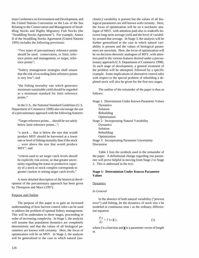
Comparing the above with Equation (3) shows thatuse of a logarithmic control rule does not alter the un-derlying stock dynamics in any qualitative way. TheGompertz-Fox model corresponds to the special case ofthe above in which d=0. Examples of logarithmic con-trol rules are shown in Figure 1.

Solution

In General

The time trajectory of stock size will generally be

of the form t ,x , ,x )( 0ωχ , where x0 represents an initial

condition and t is measured with respect to an initialtime t

0=0. In the limit as t approaches infinity, the tra-

jectory will converge to the equilibrium value ,x )(* ωχ ,assuming such an equilibrium exists.

For Example

The equilibrium stock size implied by Equation (4)is given by

e = d ,c ,b ,axd + a

c - b + a ))(ln(1

)(*

and the time trajectory is given by

d ,c ,b ,ax

x d ,c ,b ,ax

= t ,x ,d ,c ,b ,ax

e t d + a -

)(

)(

)(

*0*

0

)(

. (5)

For the special case c=d=0 (i.e., no fishing), theequilibrium stock size is simply be.

Figure 1. Example control rules. In each of the upper panels, the slope of the control rule increases directlywith d. In each of the bottom panels, the height of the control rule increases directly with c.

0

0.1

0.2

0.3

0 0.5 1 1.5 2

Stock Size

Fis

hing

Mor

talit

y R

ate

c = 0.05

0

0.1

0.2

0.3

0 0.5 1 1.5 2

Stock Size

Fis

hing

Mor

talit

y R

ate

c = 0.15

0

0.1

0.2

0.3

0 0.5 1 1.5 2

Stock Size

Fis

hing

Mor

talit

y R

ate

d = 0.05

0

0.1

0.2

0.3

0 0.5 1 1.5 2

Stock Size

Fis

hing

Mor

talit

y R

ate

d = 0.15

129


Rebuilding

In General

In practice, fish stocks are often observed to be atlevels of abundance well below those considered to beoptimal, or even safe. In such situations, fisheries sci-entists are frequently asked to estimate how much timewill elapse before the stock rebuilds to some referencelevel, contingent upon implementation of a specifiedharvest policy in the interim. More proactively, the “re-building” question may be phrased this way: How lowcan a stock’s level of abundance fall and still rebuild toa size x

reb within a time period t

reb under a specified har-

vest policy? This is not the only issue which a rebuild-ing plan might logically address (e.g., Powers 1996),but it is a central one (e.g., as implied by U.S. Depart-ment of Commerce 1998). The answer is obtained bysolving the equation rebrebthr x = tx , ,x ),( ωχ for the“threshold” stock size x

thr.

For Example

Setting Equation (5) equal to xreb

, setting t=treb

, andsolving for x

0 (relabeled x

thr) gives

) d ,c ,b ,(ax

x d ,c ,b ,ax = x reb

thr

e treb d + a

*

*

)(

)( .

In the special case where xreb

=b, the above simpli-fies to

- e d + a

b d - c - a - b = x

treb d + athr

1

)(lnexp

)(

(6)

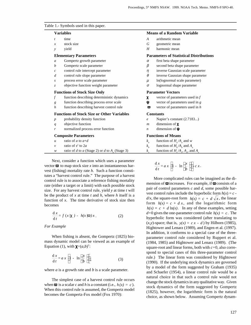
Examples of logarithmic harvest control rules andtheir corresponding stock size thresholds for parametervalues a=0.2, b=10, x

reb=10, and t

reb=10 are shown in

Figure 2. In each of Figure 2’s four panels, the upper-most control rule passes through the point (b,a), indi-cated by the intersection of the horizontal dotted lineand the rightmost vertical dotted line. Whenever x

reb=b,

any harvest control rule passing through the point (b,a),meaning any control rule in which h(b)=a, will alwayshave a threshold stock size equal to b. Furthermore,control rules in which h(b)<a will always have a thresh-old stock size less than b in such cases (i.e., wheneverx

reb=b).

Figure 2. Example control rules (solid curves) and associated thresholds (vertical dotted lines). In each panel,as c decreases, the control rule moves down and the threshold moves left.

0

0.1

0.2

0.3

0 5 10 15 20

Stock Size

Fis

hing

Mor

talit

y R

ate

d = 0

0

0.1

0.2

0.3

0 5 10 15 20

Stock Size

Fis

hing

Mor

talit

y R

ate

d = 0.05

0

0.1

0.2

0.3

0 5 10 15 20

Stock Size

Fis

hing

Mor

talit

y R

ate

d = 0.10

0

0.1

0.2

0.3

0 5 10 15 20

Stock SizeF

ishi

ng M

orta

lity

Rat

e

d = 0.15

130

Optimization

In General

Sustainable (equilibrium) yield can be viewed as afunction of the parameter vectors χχχχχ and ωωωωω. To keepthings relatively simple throughout the remainder of thepaper, let the control parameter c correspond to the ithelement of ωωωωω and let ωωωωω( i )

denote the vector ωωωωω with theith element (i.e., c) removed, and let sustainable yieldbe written ) , ( ) (ωχ i

* | cy to emphasize the dependence ofsustainable yield on c. Then, MSY is achieved condi-tionally on χχχχχ and ωωωωω( i )

by finding the value ) , () (MSY

ωχi

csuch that the following equation is satisfied:

0 = | d

) , | ( d) , ( = ) (MSY

) (*

ωχωχ

i

i

ccc

cy.

For Example

The sustainable yield corresponding to Equation (4)is given by substituting ) , , , (* dcbax into the loga-rithmic control rule, giving

( )

d + a

c - b + a

d + a

c - b + a d + c =

d ,c ,b ,ax d ,c ,b ,(ax d + c = d ,b ,a | cy

))(ln(1exp

))(ln(1

)())(ln)( ***

.

Given a value of either of the control parameters cand d, it is possible to solve for the value of the other sothat sustainable yield is maximized. For example, if thesolution is conditioned on control parameter d, MSY isobtained by setting

)(ln)(MSY

b d - a = d ,b ,a c .

Thus, an “MSY control rule” for this model is anyrule of the form

)(ln)()( MSY x d + d ,b ,a c = d ,b ,a|xh

(cf. U.S. Department of Commerce 1998). In Figure 2,for example, the uppermost curve in each panel is anMSY control rule. The Gompertz-Fox model corre-sponds to the special case where d=0, giving

a = ,b ,a c 0)(MSY . Changing the value of d allows theMSY control rule to be viewed as a continuum extend-ing from a constant fishing mortality policy at one end(d=0) to a constant escapement policy at the other end(in the limit as d approaches infinity).

For any MSY control rule of the above form, equi-librium stock size is equal to b. MSY itself is equal tothe product ab, and is thus independent of d.

Stage 2: Incorporating Natural Variability

Dynamics

In General

Equation (2) can be generalized to a stochastic dif-ferential equation incorporating random natural variabil-ity as follows:

)|( - )( )|( + )|( = d

dxxhtrxgxf

t

x ωψχ , (7)

where r(t) is a standard white noise process and g is afunction of x, with parameter vector ψψψψψ of length n, thatscales the intensity of the noise. It should be noted thatthe interpretation of stochastic differential equationsgiven by Stratonovich (1963) is used here (e.g., Ricciardi1977).

For Example

Natural variability can be added to the determinis-tic Gompertz model with a logarithmic harvest control

rule by setting ψψψψψ=s, sx|xg =) ( ψ and recasting the timederivative as a stochastic differential equation of the form

( )x x d + c - tr x s+ b

x - x a =

t

x )ln()(ln1

d

d

. (8)

Solution

In General

Broadly speaking, stock size at time t could poten-tially range anywhere from zero to arbitrarily large,though some stock sizes are more probable than others.Given an initial condition x

0, this fact can be modeled as

a pdf with parameter vector (χχχχχT, ψψψψψT, ωωωωωT, x0, t)T. More

precisely, the probability that stock size falls between x1

and x2 at time t may be written in terms of the “transi-

tion distribution” )( 0 t ,x , , , | xpx ωψχ as follows:

x t ,x , , , | xp = x tx xPr xxx d)())(( 02121 ωψχ∫≤≤ .

In the limit as t approaches infinity, px (if it still

exists) describes the “stationary distribution” of x. Thestationary distribution can be written )(* ωψχ , , | xpx .

For Example

Using a different parametrization, the solution toEquation (8) was considered for the special case c=d=0(i.e., no harvesting) by Capocelli and Ricciardi (1974).The less restricted case d=0 (with c arbitrary) was con-sidered by Thompson (1998). When no restrictions areplaced on either c or d, the stationary distribution of

131


stock size is lognormal, specifically,

d , s ,a

d c, ,b ,a - x -

x d , s ,a

=d ,c , s ,b ,a | xp

x

x

x

x

×

)(

)()(ln

2

1exp

)(

1

2

1

)(

*

* 2

*

*

σµ

σπ

,

where

( ))(ln))(ln(1

)( ** d ,c ,b ,ax = d + a

c - b + a = d c, ,b ,axµ

and

) d + (a

s = d , s ,ax

2)(*σ .

Similarly, the transition distribution of stock size attime t is also lognormal, specifically,

×

t ,d , s ,a

t ,x ,d ,c ,b ,a - x-

x t ,d , s ,a

= t ,x ,d ,c , s ,b ,a | xp

x

x

x

x

)(

)()(ln

2

1exp

)(

1

2

1

)(

0

2

0

σµ

σπ

(9)

where

( ) ) , , , ( e - 1

+ )ln( e = ), , , , , (*

00*

) + ( -

) + ( -

dcba

x txdcba

x

x

tda

tda

µ

µ

and

d , s ,a e - = t ,d , s ,a xxt d + a- )(1)( *)2( σσ .

Rebuilding

In General

In the presence of natural variability, discussion ofrebuilding trajectories can become much more compli-cated than in the deterministic case. Because an infinitenumber of rebuilding trajectories is possible in the sto-chastic case, rebuilding is typically described using somesort of summary statistic. For example, the followingequation could be solved for x

thr after substituting some

desired probability of successful rebuilding (e.g., 50%)for the left-hand side:

xtx | xp = tx x rebthrxrebrebreb xd ) , , , , ())((Pr ωψχ∫∞≤≤ ∞

.

Alternatively, the solution could be expressed interms of expected values of x (or some transformationthereof) at time t=t

reb , for example, by equating x

reb with

the arithmetic mean or geometric mean of x at time t=treb

.

For Example

Unlike the general case, a fortunate property of themodel used here is that consideration of rebuildingschedules in the presence of natural variability need notbe any more complicated than in the deterministic situ-ation described in Stage 1, depending on the choice ofsummary statistic. Because the geometric mean of thetransition distribution [Equation (9)] is identical to thedeterministic solution of the time trajectory [Equation(5)], and because the lognormal form of the transitiondistribution implies that the geometric mean is equal tothe median, using either the geometric mean or a 50%probability of exceeding x

reb to compute the threshold

stock size xthr

gives the same result as in the determinis-tic case [Equation (6)].

Optimization

In General

The conditional arithmetic mean of the stationarydistribution of yield is defined as

xxpxyA *xy d ) , , | ( ) | ( = ) , , ( 0 ωψχωωψχ ∫

∞ .

The dependence of the conditional arithmetic meanon a particular control parameter can be emphasized byrewriting ) , , ( ωψχyA as ) , , ( )(iy | cA ωψχ , followingthe Stage 1 convention in which control parameter ccorresponds to the ith element of ωωωωω. Then, this quantitycan be maximized with respect to control parameter cby differentiating, setting the resulting expression equalto zero, and solving with respect to c. Maximizing

), , ( )(iy | cA ωψχ with respect to c gives the control pa-rameter value associated with maximum expected sta-tionary yield (MESY):

0 = | d

) , , | ( d) , , ( ~ = )(MESY

)(

iccc

cA iyωψχ

ωψχ,

where use of the “~” symbol is intended to denote thatthe maximization is conducted with respect to the con-ditional mean (alternative maximizations will be de-scribed later).

Much of the literature concerning optimal harveststrategies in the presence of natural variability deals withtradeoffs between the magnitude of yield on averageand the variability about that average. In the context ofcomparisons between the classical one-parameter har-vest policies, such tradeoffs have been considered byRicker (1958), Larkin and Ricker (1964), Gatto andRinaldi (1976), Beddington and May (1977), May et al.(1978), Reed (1978), Hilborn (1979), Hilborn and

132

Walters (1992), Frederick and Peterman (1997), andSteinshamn (1998). In the context of optimal controlpolicies, they have been considered by Walters (1975),Mendelssohn (1980), and Horwood et al. (1990). In thecontext of fixed-form control rules, they have been con-sidered by Allen (1973), Aron (1979), Hilborn (1985),Ruppert et al. (1985), Getz et al. (1987), Hightower andLenarz (1989), Hightower (1990), Quinn et al. (1990),Zheng et al. (1993), and Engen et al. (1997).

One way to characterize the variability of yield ona scale equivalent to that of the arithmetic mean is bythe standard deviation. If c is set equal to

, ) , , (~) (MESY ωψχ ic both the arithmetic mean and standard

deviation of the stationary distribution of y will be func-tions of χχχχχ, ψψψψψ, and ωωωωω( i )

, meaning that tradeoffs betweenthe arithmetic mean and standard deviation can beviewed as a function of the control parameter sub-vec-tor ωωωωω( i )

for given values of χχχχχ and ψψψψψ.

For Example

By defining a natural variability level

a s = ,s ,a v

x 2)0(

22*σ≡

(i.e., by defining v as the variance of the stationary dis-tribution of log stock size when d=0), the equations formany quantities of interest in the example model can besimplified considerably. Thus, wherever s appears as aparameter in a particular equation, it can be replacedwith the quantity 2av, and whenever s appears as afunction argument in a particular equation, it can be re-placed with the parameter v. Similarly, by defining ascaled control parameter

a

d w≡

(i.e., by viewing the control parameter d relative to arather than in absolute terms) and reparametrizing ac-cordingly, it turns out that a appears only as a constantof proportionality in many (but not all) quantities of in-terest in this model. Thus, wherever d appears as a pa-rameter in a particular equation, it can be replaced withthe quantity wa, and wherever d appears as a functionargument in a particular equation, it can be replaced withthe parameter w.

With these composite parameters, the conditionalarithmetic mean of the stationary distribution of stocksize x can be written as

∫∞

wa

cvb

wa

c

w

x w ,c ,v ,b ,a | xp x = w ,c ,v ,b ,aA xx

- 2

+ )ln( + 1 + + 1

1 exp =

d)()( *0

,

and the conditional arithmetic mean of the stationarydistribution of yield y can be written as

( )

×

∫∞

wa

cvb

wa

c

w

vbwa

c

wwa

wcvbaAvbwa

c

wwa

x wc, v, b, a, | xp x x d + c = wc, v, b, a,A

x

xy

-2

+ )ln( +1 + +1

1exp

+ )ln( +1 + +1

1 =

) , , , ,( + )ln( +1 + +1

1 =

d)()(ln)( *0

(10)

Given w, the value of c that maximizes expectedstationary yield is

( )a wv + b - = w ,v ,b ,a c ))(ln(1 )(~MESY . (11)

Note that )(~MESY w ,v ,b ,a c approaches

)(MSY w ,b ,a c as v approaches zero. Also, in the specialcase where w=0, the solution simplifies to

a = ,b ,ac = ,v ,b ,ac 0)(0)(~MSYMESY regardless of the

value of v. Generally, then, the stochastic equivalent ofan MSY control rule (without considering parameteruncertainty) is given by the MESY control rule

)(ln)(~)(~

MESYMESY x wa+ w ,v ,b ,a c = w ,v ,b ,a | x h .

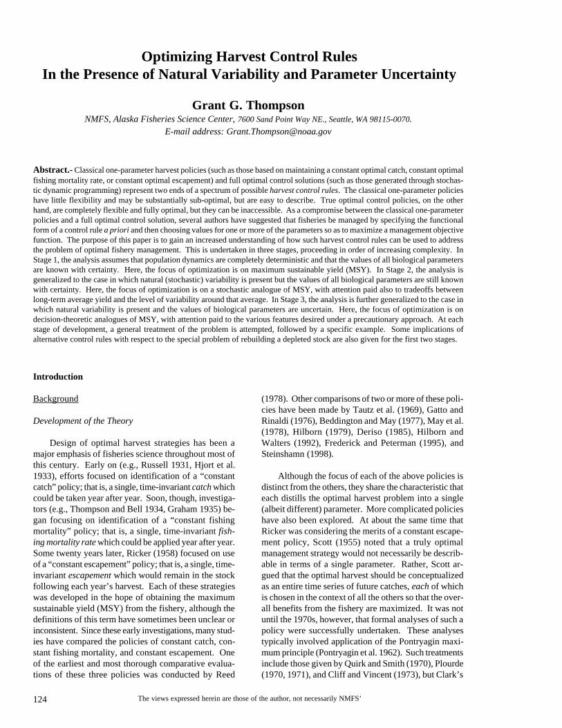
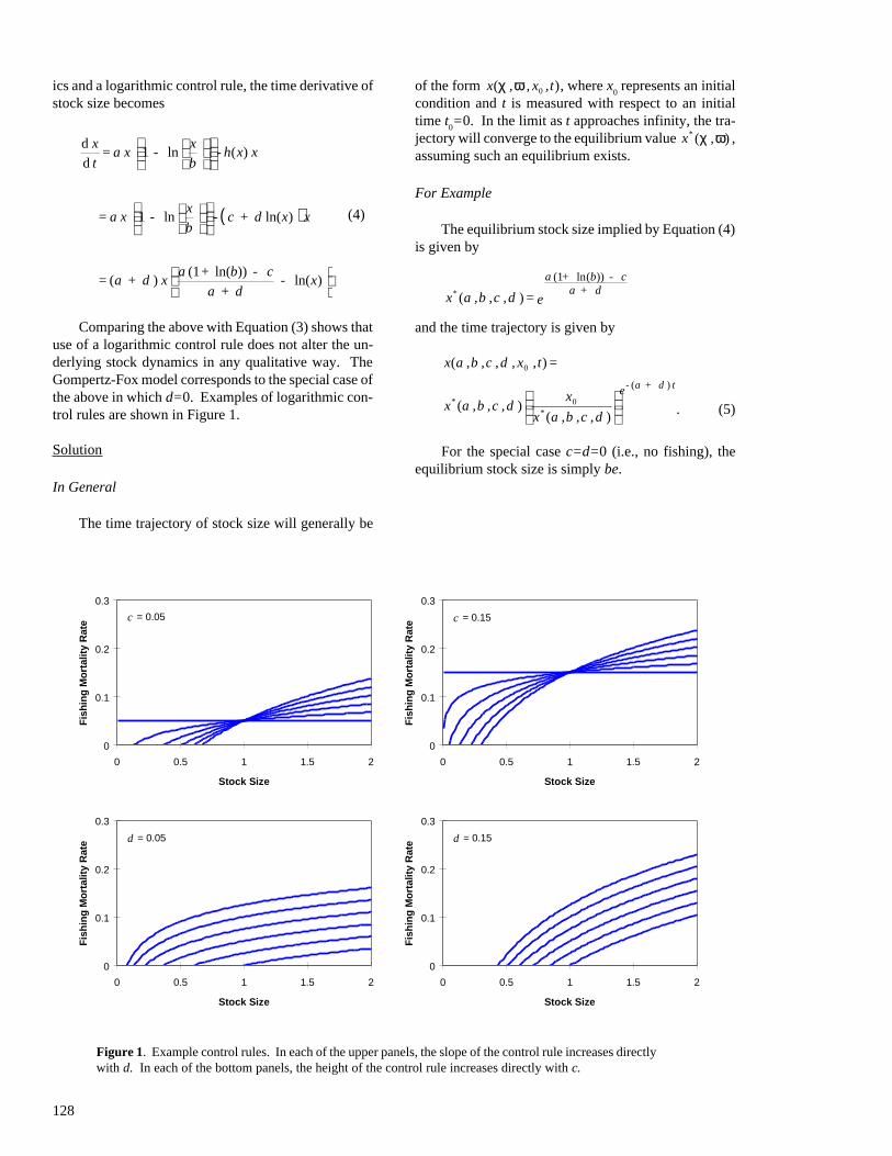
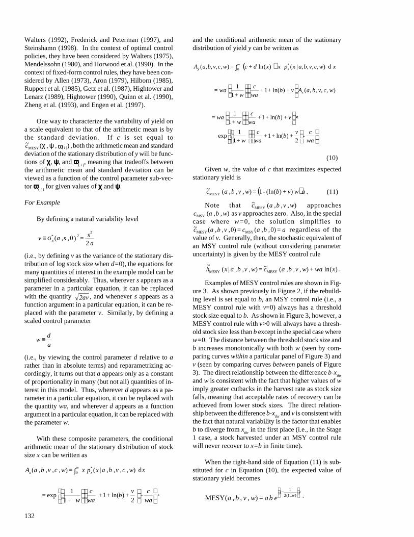
Examples of MESY control rules are shown in Fig-ure 3. As shown previously in Figure 2, if the rebuild-ing level is set equal to b, an MSY control rule (i.e., aMESY control rule with v=0) always has a thresholdstock size equal to b. As shown in Figure 3, however, aMESY control rule with v>0 will always have a thresh-old stock size less than b except in the special case wherew=0. The distance between the threshold stock size andb increases monotonically with both w (seen by com-paring curves within a particular panel of Figure 3) andv (seen by comparing curves between panels of Figure3). The direct relationship between the difference b-x

thr

and w is consistent with the fact that higher values of wimply greater cutbacks in the harvest rate as stock sizefalls, meaning that acceptable rates of recovery can beachieved from lower stock sizes. The direct relation-ship between the difference b-x

thr and v is consistent with

the fact that natural variability is the factor that enablesb to diverge from x

thr in the first place (i.e., in the Stage

1 case, a stock harvested under an MSY control rulewill never recover to x=b in finite time).

When the right-hand side of Equation (11) is sub-stituted for c in Equation (10), the expected value ofstationary yield becomes

vwebawvba

+

−)1(2

11

= ) , , , (MESY .

133


Figure 3. Example MESY control rules (solid curves) and associated thresholds (vertical dotted lines). In eachpanel, as w increases (with c implicit), the slope of the control rule increases and the threshold moves left.

0

0.1

0.2

0.3

0 5 10 15 20

Stock Size

Fis

hing

Mor

talit

y R

ate

v = 0.1

0

0.1

0.2

0.3

0 5 10 15 20

Stock Size

Fis

hing

Mor

talit

y R

ate

v = 0.2

0

0.1

0.2

0.3

0 5 10 15 20

Stock Size

Fis

hing

Mor

talit

y R

ate

v = 0.3

0

0.1

0.2

0.3

0 5 10 15 20

Stock Size

Fis

hing

Mor

talit

y R

ate

v = 0.4

Unlike the deterministic case where MSY was in-dependent of the control parameter d, MESY does de-pend on the value of d, through the latter’s dependenceon w. The exponent in the above equation reaches aminimum of v/2 when w=0 and a maximum of v as wapproaches infinity.

When )(~MESY w ,v ,b ,a c = c , the standard deviation

of stationary yield can be written

wv

v evw

ww v

w

wbea

wvba

+−

1 -

+ 1 +

+ 1

+ 2 + 1

= ) , , , (SDSY

2

2

.

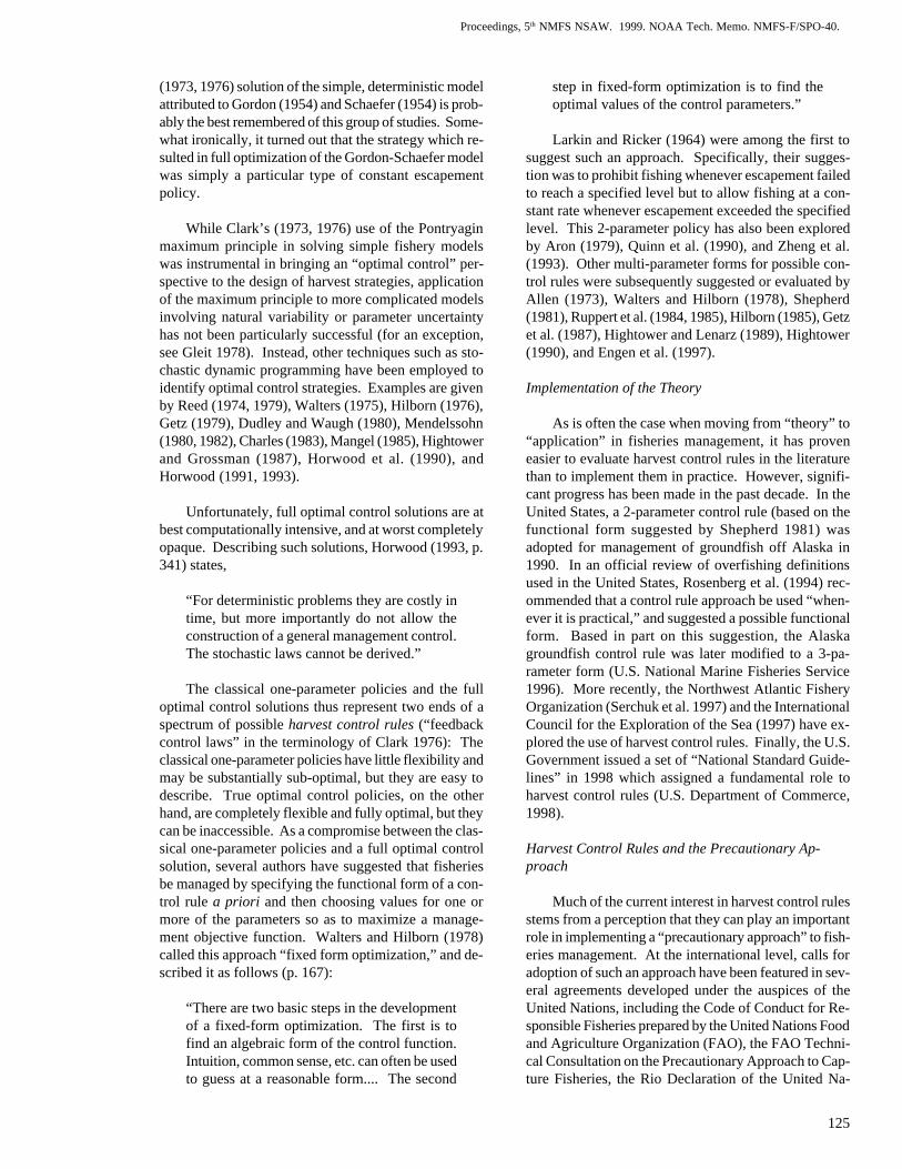
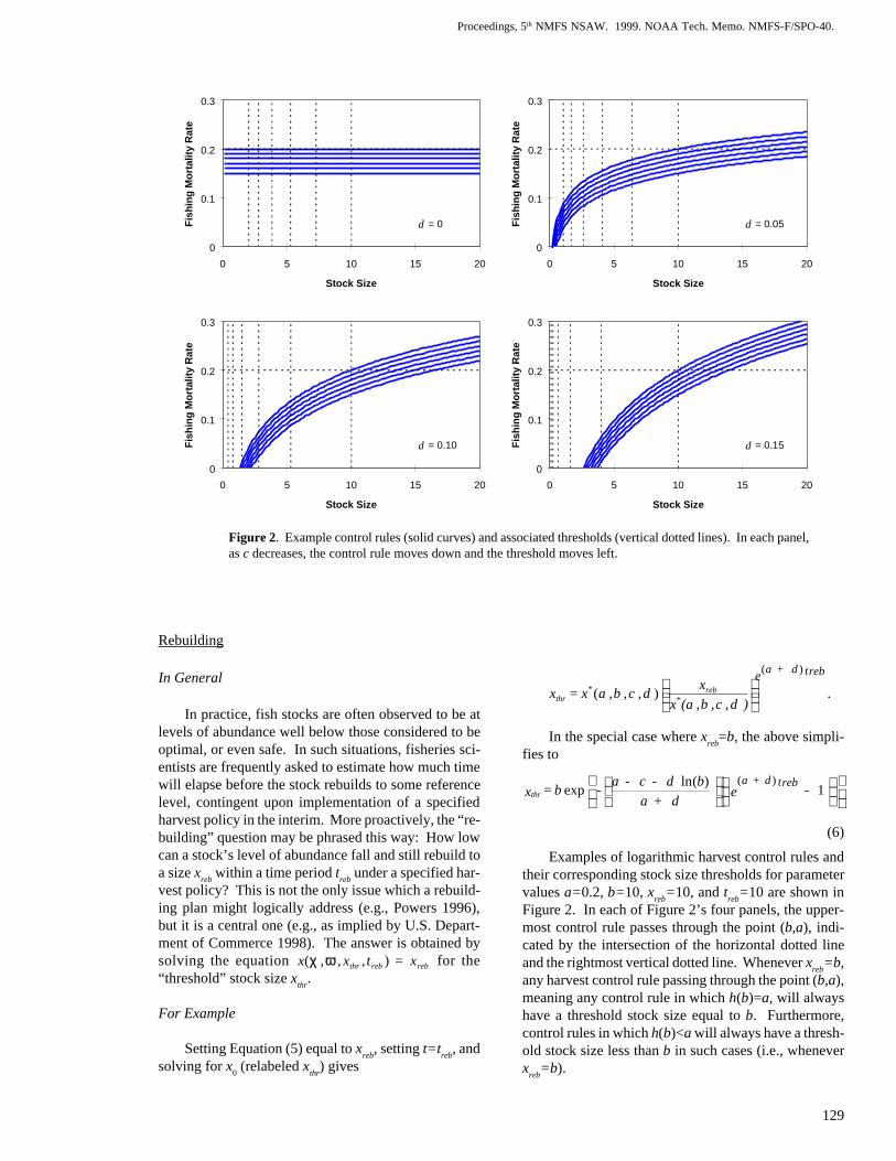
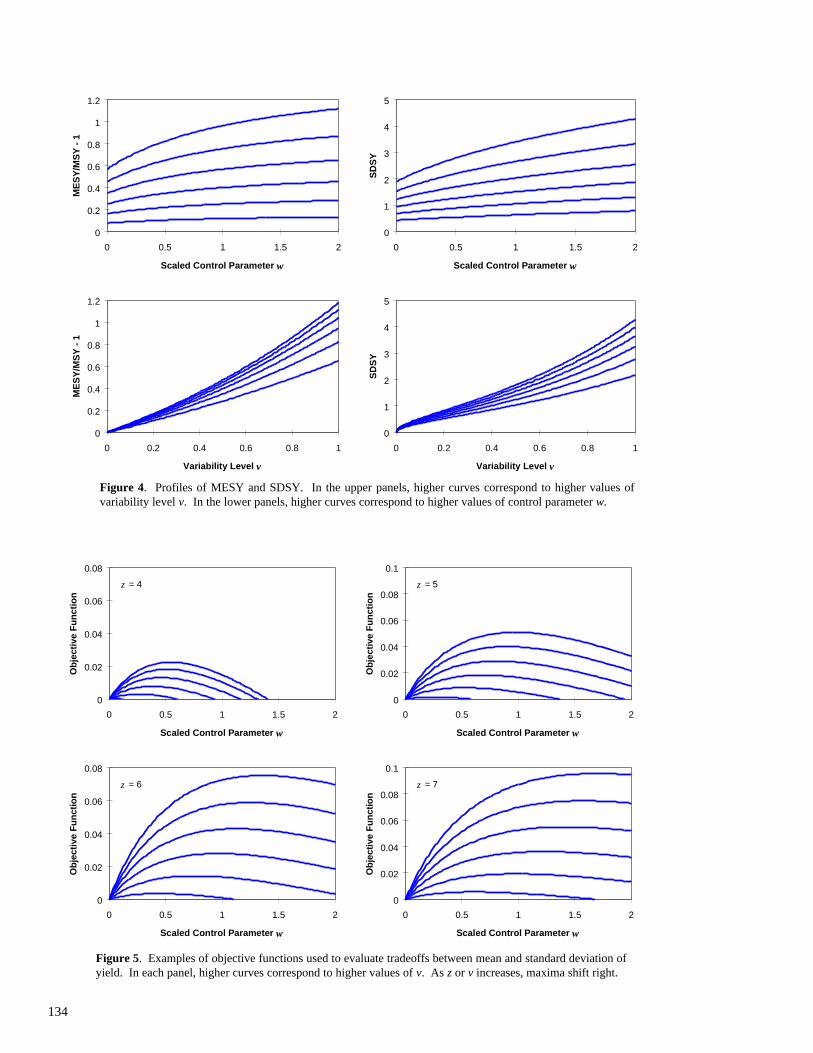
The term under the square root symbol reaches aminimum of 1-e-v when w=0 and increases without limitas w approaches infinity. MESY (expressed as a pro-portionate increase over MSY) and SDSY are plottedfor a=b=1 and several values of v and w in Figure 4.

In managing a fishery, suppose that any increase inMESY were viewed as a desirable result (all other thingsbeing equal), and that likewise any decrease in SDSYwere viewed as a desirable result (all other things beingequal). Because both MESY and SDSY increase mono-tonically but nonlinearly with w, it may be possible tofind an optimal value for w depending on the prefer-

ence associated with a unit increase in MESY relativeto the preference associated with a unit decrease inSDSY. For example, suppose that the goal was to choosethe value of the control parameter w so as to maximizethe following objective function, which uses the param-eter z to form a linear combination of MESY and (nega-tive) SDSY:

1 - -1 -

- +1

+ +1

+ 2 +1 - e

=

1 - 0) , , , (SDSY - 0) , , , (MESY

) , , , (SDSY - ) , , , (MESY

- -

2

2 + 1

- + 1

-

eez

evw

wvw

w

wz

vbavbaz

wvbawvbaz = w) ,q(v

vv

wv

wv

The above equation is scaled so that q(v,0)=0. Theparameter z represents the amount by which a unit in-crease in MESY is preferred relative to a unit decreasein SDSY. This objective function is plotted for severalvalues of v and z in Figure 5.

While it is not possible to obtain a closed-form so-lution for the value of w that maximizes q, it is possibleto derive the value of z for which a particular value of wwould be optimal, given v:

134

Figure 4. Profiles of MESY and SDSY. In the upper panels, higher curves correspond to higher values ofvariability level v. In the lower panels, higher curves correspond to higher values of control parameter w.

0

0.2

0.4

0.6

0.8

1

1.2

0 0.5 1 1.5 2

Scaled Control Parameter w

ME

SY

/MS

Y -

1

0

1

2

3

4

5

0 0.5 1 1.5 2


SD

SY

0

0.2

0.4

0.6

0.8

1

1.2

0 0.2 0.4 0.6 0.8 1

Variability Level v

ME

SY

/MS

Y -

1

0

1

2

3

4

5

0 0.2 0.4 0.6 0.8 1

Variability Level v

SD

SY

Figure 5. Examples of objective functions used to evaluate tradeoffs between mean and standard deviation ofyield. In each panel, higher curves correspond to higher values of v. As z or v increases, maxima shift right.

0

0.02

0.04

0.06

0.08

0 0.5 1 1.5 2


Obj

ectiv

e F

unct

ion

z = 4

0

0.02

0.04

0.06

0.08

0.1

0 0.5 1 1.5 2


Obj

ectiv

e F

unct

ion

z = 5

0

0.02

0.04

0.06

0.08

0 0.5 1 1.5 2


Obj

ectiv

e F

unct

ion

z = 6

0

0.02

0.04

0.06

0.08

0.1

0 0.5 1 1.5 2


Obj

ectiv

e F

unct

ion

z = 7

135


( )

( )

1)(12)(3

)(122(43

opt2opt

opt

optopt2opt

opt

opt

opt2opt

3opt

opt

11

1

- e w+ + e vw + wv + + w

w+ - e + wv) + + w + w

= v)|z(w

w+ v

w+ v

w+ v

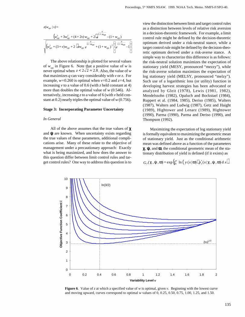
The above relationship is plotted for several valuesof w

opt in Figure 6. Note that a positive value of w is

never optimal when 8.222 ≈<z . Also, the value of wthat maximizes q can vary considerably with v or z. Forexample, w=0.260 is optimal when v=0.2 and z=4, butincreasing v to a value of 0.6 (with z held constant at 4)more than doubles the optimal value of w (0.546). Al-ternatively, increasing z to a value of 6 (with v held con-stant at 0.2) nearly triples the optimal value of w (0.756).

Stage 3: Incorporating Parameter Uncertainty

In General

All of the above assumes that the true values of χχχχχand ψψψψψ are known. When uncertainty exists regardingthe true values of these parameters, additional compli-cations arise. Many of these relate to the objective ofmanagement under a precautionary approach: Exactlywhat is being maximized, and how does the answer tothis question differ between limit control rules and tar-get control rules? One way to address this question is to

view the distinction between limit and target control rulesas a distinction between levels of relative risk aversionin a decision-theoretic framework. For example, a limitcontrol rule might be defined by the decision-theoreticoptimum derived under a risk-neutral stance, while atarget control rule might be defined by the decision-theo-retic optimum derived under a risk-averse stance. Asimple way to characterize this difference is as follows:the risk-neutral solution maximizes the expectation ofstationary yield (MESY, pronounced “mezzy”), whilethe risk-averse solution maximizes the expectation oflog stationary yield (MELSY, pronounced “melzy”).Such use of a logarithmic loss (or utility) function indeveloping harvest strategies has been advocated oranalyzed by Gleit (1978), Lewis (1981, 1982),Mendelssohn (1982), Opaluch and Bockstael (1984),Ruppert et al. (1984, 1985), Deriso (1985), Walters(1987), Walters and Ludwig (1987), Getz and Haight(1989), Hightower and Lenarz (1989), Hightower(1990), Parma (1990), Parma and Deriso (1990), andThompson (1992).

Maximizing the expectation of log stationary yieldis formally equivalent to maximizing the geometric meanof stationary yield. Just as the conditional arithmeticmean was defined above as a function of the parametersχχχχχ, ψψψψψ, and ωωωωω, the conditional geometric mean of the sta-tionary distribution of yield is defined (if it exists) as

( )( )xxpxy(G*xy d ) , , | ( ) | ( ln exp = ) , , 0 ωψχωωψχ ∫∞ .

Figure 6. Value of z at which a specified value of w is optimal, given v. Beginning with the lowest curveand moving upward, curves correspond to optimal w values of 0, 0.25, 0.50, 0.75, 1.00, 1.25, and 1.50.

0

1

2

3

4

5

6

7

8

9

10

0 0.2 0.4 0.6 0.8 1 1.2 1.4 1.6 1.8 2

Variability Level v

Obj

ectiv

e F

unct

ion

Coe

ffici

ent

z

2x21/2

ln(3/2)

136

Likewise, in a manner analogous to that used todevelop the conditional MESY solution, ) , , ωψχ(Gy

can be rewritten as ) , , )(ωψχ i y | (cG and then maxi-mized with respect to c, giving the control parametervalue associated with the maximum expected log sta-tionary yield, conditional on χχχχχ, ψψψψψ, and ωωωωω( i )

:

0 = | d

) , , |( d),,(~

)(

) (

MELSY i

iy

ccc

c Gωψχ

ωψχ= .

However, when the values of χχχχχ and ωωωωω are uncer-tain, maximization of the mean (either arithmetic or geo-metric) of the conditional pdf is not particularly helpfulby itself, as the solution is a function of parameters whosevalues are unknown. Rather, it is the moments of themarginal pdf that are of interest. For example, the arith-metic mean of the marginal pdf is defined as

... ...

A

A

nm

y

y

ψψχχ dddd

) , (p ) , , (

... ... = )(

11

,

----

ψχωψχ

ω

ψχ

∫∫∫∫ ∞∞

∞∞

∞∞

∞∞

.

Rewriting the above as )( )(iy |cA ω and maximiz-ing with respect to c gives )( )(MESY i c ω ; that is,

0 = | d

)|( d)(

)(

)(

MESY i

iy

ccc

cAω

ω= .

The above derivation involves two operations: in-tegration and differentiation. The order in which thesetwo are performed can make a difference (though per-haps not always). In the above, integration precedesdifferentiation. In other words, the arithmetic mean ofthe marginal distribution of stationary yield is computedconditionally on c, then c is chosen so as to maximizethis expectation. An alternative approach would be tochoose the value of c that maximizes expected station-ary yield conditional on χχχχχ, ψψψψψ, and ωωωωω( i )

, and then com-pute the expectation of this value. This is accomplished

by multiplying ) , , (~)(MESY i c ωψχ by ) , (, ψχψχp and in-

tegrating over the elements of χχχχχ and ψψψψψ, giving

... ...

pc

c

nm

i

i

ψψχχ dddd

) , ( ) , , ( ~

... ... = )(

11

,)(MESY

----)(MESY

ψχωψχ

ω

ψχ

∫∫∫∫ ∞∞

∞∞

∞∞

∞∞

.

The same procedure can be followed for the geo-metric mean. The geometric mean of the marginal pdfis defined as

( )

∫∫∫∫∞∞

∞∞

∞∞

∞∞

... ...

pGG

nm

yy

ψψχχ dddd

) , ( ) , , (ln

... ...

exp = )(

11

,

----

ψχωψχω ψχ .

Rewriting the above as )( )(iy |cG ω and maximizing

with respect to c gives ; )( )(MELSY i c ω that is,

0 =| d

) | ( d)(

)(

)(

MELSY i

iy

ccc

cGω

ω= ,

while multiplying ) , , (~)(MELSY i c ωψχ by ) , (, ψχψχp and

integrating over the elements of of χχχχχ and ψ ψ ψ ψ ψ gives

... ...

pc

c

nm

i

i

ψψχχ dddd

) , ( ) , , ( ~

... ... = )(

11

,)(MELSY

----)(MELSY

ψχωψχ

ω

ψχ

∫∫∫∫ ∞∞

∞∞

∞∞

∞∞

.

Thus, there are a number of alternative ways to pro-ceed. In either the MESY case or the MELSY case, atleast three solutions can be envisioned: 1) consideringuncertainty due to natural variability only, solve for theoptimum value of c as a function of the parameters χχχχχ, ψψψψψ,ωωωωω( i )

, then evaluate that solution at the “best” estimate ofthose parameters (the “solve-then-evaluate” method); 2)considering uncertainty due to natural variability only,solve for the optimum value of c as a function of theparameters χχχχχ, ψψψψψ, ωωωωω( i )

, then take the expectation of thatsolution over the parameters χχχχχ and ψψψψψ (the “solve-then-integrate” method); and 3) considering both natural vari-ability and parameter uncertainty, solve for the optimumvalue of c (the “integrate-then-solve” method). Thesethree solutions are summarized in the table below:

Attitude Solutiontoward risk Solution technique notationrisk neutral solve-then-evaluate ) , , ( ~

)(MESY ic ωψχrisk neutral solve-then-integrate )( )(MESY ic ωrisk neutral integrate-then-solve )( )(MESY ic ωrisk averse solve-then-evaluate ) , , (~

)(MELSY ic ωψχrisk averse solve-then-integrate )( )(MELSY ic ωrisk averse integrate-then-solve )( )(MELSY i c ω

For Example

In Stage 2, the quantity w (defined as w≡d/a) was aconstant. To retain the interpretation of w as a constantin Stage 3, it will prove convenient at this point to rede-fine w≡d/A

a and to reparametrize the model accordingly.

Thus, wherever w appears as a parameter in a previousequation, it can be replaced with the quantity A

aw/a. Use

of the redefined parameter w renders many quantities ofinterest in this model proportional to A

a.

A general solution for cMESY

(w)cannot be obtained,because any particular solution will depend on the formof the joint pdf of a, b, and v. However, because

)( ~MESY w ,v ,b ,ac is linear in a, ln(b), and v [Equation

(11)], the following solution for )(MESY w c will be inde-pendent of the form of the joint pdf of a, b, and v:

( )( ) avb A w A + G - = w c )(ln1)(MESY (12)

137


Obtaining general solutions for MELSY is evenmore difficult than in the MESY case. For one thing,the fact that the logarithmic control rule forces yield toequal zero at x=exp(-c/d) means that )( w ,c ,v ,b ,aGy

does not exist except when w=0. For purposes of illus-tration, however, an exact solution for a quantity closelyrelated to c

MELSY(w) can be obtained if a, b, and v are

assumed to be independent and if particular functionalforms are chosen for their respective pdfs. Specifically,let p

a(a) follow a 3-parameter F distribution with scale

parameter d, let pb(b) follow a lognormal distribution,

and let pv(v) follow an inverse Gaussian distribution (Ap-

pendix).

For any positive random variable, the ratio of theharmonic mean to the arithmetic mean may be viewedas a measure of the degree of certainty surrounding thevalue of that variable. This ratio ranges from a lowerbound no less than zero, representing complete uncer-tainty, to an upper bound no greater than unity, repre-senting complete certainty (e.g., Mitrinovi� et al. 1993).For the particular distributional forms assumed here, theratios of harmonic to arithmetic means may be expressedin terms of the coefficient of variation (CV) as follows(the harmonic and arithmetic means are also given asfunctions of their respective distributional parametersin the Appendix):

. +

= A

H

, +

= A

H

, + w+

w- + w+ =

A

H

vv

v

bb

b

a

a

a

a

2

2

2

2

CV1

1

CV1

1

CV21

CV )(1 1

Given the assumption that a follows an F distribu-tion with scale parameter d, the quantity u≡a/(a+d) isbeta-distributed with arithmetic mean

w + w + A

H

w+ A

H

= A

a

a

a

a

u22.

Then, a quantity closely related to cMELSY

(w) can bewritten (Appendix) as

( )( ) avvbba A w kA + kG - k = w c )(ln)(ˆMELSY , (13)

where

, A

H =k

, w+

w+ A

H = k

b

bb

a

aa

A - u

1

1

A -

A

H A - = k u

v

v

-

v

-

v 111 2

1

.

For all practical purposes, the adjustment factorsk

a, k

b, and k

v vary directly with the ratios H

a/A

a, H

b/A

b,

and Hv/A

v, respectively, so that an increase in uncertainty

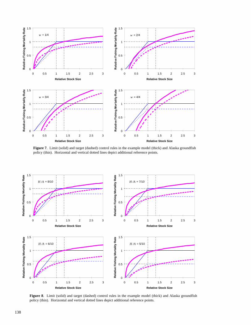
regarding any of the parameters results in a downwardshift in the control rule. Examples of limit control rules(using Equation (12)) and target control rules (usingEquation (13)) are shown in Figure 7 for four values ofw, in Figure 8 for four values of H

a/A

a = H

b/A

b = H

v/A

v,

and in Figure 9 for four values of Av (because the axes

in Figures 7-9 are scaled relative to Aa and G

b, the curves

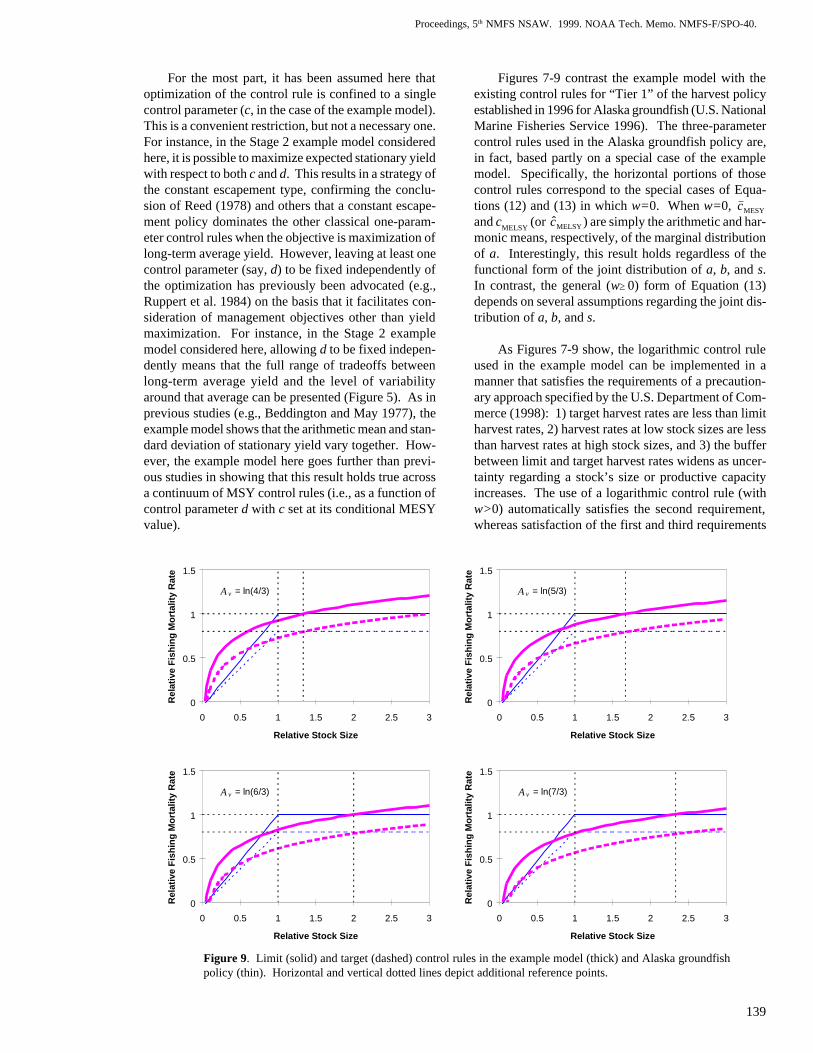
are independent of these two parameters). The upperleft panels of Figures 7-9 are all identical, giving a com-mon point of reference against which to contrast resultsassociated with different parameter values. In each ofthese figures, the control rules developed under thismodel are contrasted with the existing control rules for“Tier 1” of the harvest policy established in 1996 forAlaska groundfish (U.S. National Marine Fisheries Ser-vice 1996).

Discussion

Harvest control rules provide a tractable and heu-ristic means of comparing alternative fishery manage-ment strategies. They can be analyzed in the context ofa wide variety of models, ranging from simple deter-ministic models with known parameter values to com-plex stochastic models with uncertain parameter values.Moving from the classical one-parameter control rules(e.g., constant fishing mortality, constant escapement)to a two-parameter control rule such as the logarithmicform considered in the example model here can some-times render comparisons between the former moremeaningful by framing them as special cases along acontinuum of possible strategies rather than as concep-tually unrelated policies. More elaborate functionalforms, in which various two-parameter control rulesmight emerge as special cases, can also be imagined.Generally, the ideal level of complexity to build into aharvest control rule, as well as the appropriate numberof parameters to be left free therein, remain open ques-tions. Relative to a full optimal control solution, somedegree of optimality may be sacrificed whenever thefunctional form of the control rule is constrained a priori.However, the sacrifice may be slight. For example, inthe deterministic Gordon-Schaefer model considered byClark (1976), the optimal control solution consisted ofa one-parameter constant escapement policy. Even whenmore complicated stochastic models are used, the dif-ference between a full optimal control solution and afixed-form optimization can be negligible (e.g.,Mendelssohn 1980, Horwood 1993).

138

Figure 8. Limit (solid) and target (dashed) control rules in the example model (thick) and Alaska groundfishpolicy (thin). Horizontal and vertical dotted lines depict additional reference points.


0

0.5

1

1.5

0 0.5 1 1.5 2 2.5 3

Relative Stock Size

Re

lati

ve

Fis

hin

g M

ort

ali

ty R

ate

w = 1/4

0

0.5

1

1.5

0 0.5 1 1.5 2 2.5 3

Relative Stock Size

Re

lati

ve

Fis

hin

g M

ort

ali

ty R

ate

w = 2/4

0

0.5

1

1.5

0 0.5 1 1.5 2 2.5 3

Relative Stock Size

Re

lati

ve

Fis

hin

g M

ort

ali

ty R

ate

w = 3/4

0

0.5

1

1.5

0 0.5 1 1.5 2 2.5 3

Relative Stock Size

Re

lati

ve

Fis

hin

g M

ort

ali

ty R

ate

w = 4/4

0

0.5

1

1.5

0 0.5 1 1.5 2 2.5 3

Relative Stock Size

Rel

ativ

e F

ishi

ng M

orta

lity

Rat

e

H /A = 8/10

0

0.5

1

1.5

0 0.5 1 1.5 2 2.5 3

Relative Stock Size

Rel

ativ

e F

ishi

ng M

orta

lity

Rat

e

H /A = 7/10

0

0.5

1

1.5

0 0.5 1 1.5 2 2.5 3

Relative Stock Size

Rel

ativ

e F

ishi

ng M

orta

lity

Rat

e

H /A = 6/10

0

0.5

1

1.5

0 0.5 1 1.5 2 2.5 3

Relative Stock Size

Rel

ativ

e F

ishi

ng M

orta

lity

Rat

e

H /A = 5/10

139


For the most part, it has been assumed here thatoptimization of the control rule is confined to a singlecontrol parameter (c, in the case of the example model).This is a convenient restriction, but not a necessary one.For instance, in the Stage 2 example model consideredhere, it is possible to maximize expected stationary yieldwith respect to both c and d. This results in a strategy ofthe constant escapement type, confirming the conclu-sion of Reed (1978) and others that a constant escape-ment policy dominates the other classical one-param-eter control rules when the objective is maximization oflong-term average yield. However, leaving at least onecontrol parameter (say, d) to be fixed independently ofthe optimization has previously been advocated (e.g.,Ruppert et al. 1984) on the basis that it facilitates con-sideration of management objectives other than yieldmaximization. For instance, in the Stage 2 examplemodel considered here, allowing d to be fixed indepen-dently means that the full range of tradeoffs betweenlong-term average yield and the level of variabilityaround that average can be presented (Figure 5). As inprevious studies (e.g., Beddington and May 1977), theexample model shows that the arithmetic mean and stan-dard deviation of stationary yield vary together. How-ever, the example model here goes further than previ-ous studies in showing that this result holds true acrossa continuum of MSY control rules (i.e., as a function ofcontrol parameter d with c set at its conditional MESYvalue).

Figures 7-9 contrast the example model with theexisting control rules for “Tier 1” of the harvest policyestablished in 1996 for Alaska groundfish (U.S. NationalMarine Fisheries Service 1996). The three-parametercontrol rules used in the Alaska groundfish policy are,in fact, based partly on a special case of the examplemodel. Specifically, the horizontal portions of thosecontrol rules correspond to the special cases of Equa-tions (12) and (13) in which w=0. When w=0, MESYcand c

MELSY (or MELSYc ) are simply the arithmetic and har-

monic means, respectively, of the marginal distributionof a. Interestingly, this result holds regardless of thefunctional form of the joint distribution of a, b, and s.In contrast, the general (w$0) form of Equation (13)depends on several assumptions regarding the joint dis-tribution of a, b, and s.

As Figures 7-9 show, the logarithmic control ruleused in the example model can be implemented in amanner that satisfies the requirements of a precaution-ary approach specified by the U.S. Department of Com-merce (1998): 1) target harvest rates are less than limitharvest rates, 2) harvest rates at low stock sizes are lessthan harvest rates at high stock sizes, and 3) the bufferbetween limit and target harvest rates widens as uncer-tainty regarding a stock’s size or productive capacityincreases. The use of a logarithmic control rule (withw>0) automatically satisfies the second requirement,whereas satisfaction of the first and third requirements


0

0.5

1

1.5

0 0.5 1 1.5 2 2.5 3

Relative Stock Size

Rel

ativ

e F

ishi

ng M

orta

lity

Rat

e

Av = ln(4/3)

0

0.5

1

1.5

0 0.5 1 1.5 2 2.5 3

Relative Stock Size

Rel

ativ

e F

ishi

ng M

orta

lity

Rat

e

Av = ln(5/3)

0

0.5

1

1.5

0 0.5 1 1.5 2 2.5 3

Relative Stock Size

Rel

ativ

e F

ishi

ng M

orta

lity

Rat

e

Av = ln(6/3)

0

0.5

1

1.5

0 0.5 1 1.5 2 2.5 3

Relative Stock Size

Rel

ativ

e F

ishi

ng M

orta

lity

Rat

e

Av = ln(7/3)

140

is achieved by basing the limit control rule on a risk-neutral optimization and the target control rule on a risk-averse optimization. The Alaska groundfish policy alsosatisfies these three requirements, with the exception thatthe size of the buffer increases directly with uncertaintyregarding productive capacity only (not stock size).

It may also be noted that the limit control rule shownfor the example model in Figures 7-9 qualifies as anMSY control rule, whereas the limit control rule used inthe Alaska groundfish policy does not. The failure ofthe limit control rule used in the Alaska groundfish policyto qualify as an MSY control rule is due to the fact thatthe presence of the descending limb was not consideredin the process of setting the height of the horizontal limb.That is, in setting the height of the horizontal limb, theoptimization was conditional on the assumption that aconstant fishing mortality policy would apply, whereasin fact such a policy applies only when the stock is aboveits MSY level.

In Stages 1 and 2, it was assumed that estimates ofthe biological parameters a, b, and s (or v) are obtain-able. In Stage 3, it was assumed that pdfs of these pa-rameters are obtainable. In practice, obtaining theseestimates or distributions will typically be a non-trivialexercise. However, the functional form of the examplemodel described here is particularly amenable to thistask. Thompson (1998) showed how a log transforma-tion of this model satisfies the assumptions of the Kalmanfilter (e.g., Harvey 1990) exactly, meaning that eithermaximum likelihood or Bayesian methods can be usedin a straightforward manner to obtain parameter esti-mates or posterior distributions of parameters (if maxi-mum likelihood is used, distributions could be obtainedby appealing to the asymptotic normality of the param-eter estimates). The model is sufficiently simple, in fact,that the maximum likelihood estimate of the determin-istic carrying capacity (=be) can be written in closedform.

The subject of rebuilding depleted stocks was con-sidered for the Stage 1 and Stage 2 cases, but not for theStage 3 case. A Stage 3 treatment should not prove tooproblematic, however, insofar as computing the geomet-ric or arithmetic mean of Equation (6) for the case wherethe values of a and b are uncertain does not appear topose any special difficulty (note that the natural vari-ability parameter s does not enter into Equation (6)).Despite the omission of a Stage 3 treatment of rebuild-ing, the results obtained under Stages 1 and 2 in the ex-ample model offer some interesting insights on their own.For example, suppose that the goal of a rebuilding pro-gram is to return a depleted stock to its deterministicMSY stock size b. In this case, the Stage 1 examplemodel indicates that the threshold stock size prescribedby any MSY control rule will also be equal to b regard-

less of the allowable time frame for rebuilding. Thus,under Stage 1 conditions, anytime a stock falls belowits deterministic MSY stock size, it will be impossibleto rebuild to the deterministic MSY level in finite timewhile fishing according to any MSY control rule. In theStage 2 example model, however, the conclusions aredifferent. Specifically, if the geometric mean of the tran-sition distribution is used to define the threshold stocksize, the threshold stock size prescribed by any MESYcontrol rule with d>0 and s>0 will always be less than bregardless of the allowable time frame for rebuilding.Thus, under Stage 2 conditions, it is possible for a stockto fall below its deterministic MSY stock size to someextent and still rebuild to the deterministic MSY levelwithin an allowable time frame while fishing accordingto a given MESY control rule. The difference in con-clusions reached under Stages 1 and 2 in this regard isdue to the fact that a Stage 1 MSY control rule evalu-ated at the point x=b always gives a harvest rate equalto a, whereas a Stage 2 MESY control rule evaluated atthe same point always gives a harvest rate less than a solong as d>0 and s>0. However, under a MESY controlrule with d=0 (i.e., a constant fishing mortality policy),even the Stage 2 example model prescribes a thresholdstock size equal to b.

Another aspect of rebuilding that was not addressedhere is the question of whether rebuilding should beviewed primarily in terms of stock size x or in terms ofrebuilding time t. In other words, is it more importantto consider the probability that the stock size will ex-ceed x

reb at time t

reb, or the probability that the time needed

for the stock size to exceed xreb

will be greater than treb

?The two approaches are not equivalent (e.g., Dennis etal. 1991).

In conclusion, some caveats are probably appropri-ate. First, the logarithmic control rule used in the ex-ample model exhibits some features that may requiregetting used to. For example, one must either interpretthe control rule as exhibiting a discontinuity at the pointwhere it crosses the x axis (making the mathematics morecomplicated), or be prepared to accept (as an approxi-mation, at least) the idea of a small negative “yield” atsufficiently low stock sizes. Also, the fact that the con-trol rule has no finite upper bound may not be appealingto some. Second, the results pertaining to the examplemodel may not extend to other models. For instance, adiscrete rather than a continuous representation of stockdynamics, other functional forms for Equation (1), orother interpretations of the stochastic differential (Equa-tion (7); for example, Ricciardi 1977) could alter theconclusions either quantitatively or qualitatively. Fi-nally, the derivation of the MELSY solution presentedin Equation (13) requires some strong assumptions. Forinstance, the assumption that the parameters a and v areindependent is problematic unless a and s happen to vary

141


together in a particular manner. Also, the form assumedfor the pdf of a implies that, for given values of H

a and

Aa, the coefficient of variation changes with the choice

of w, which is probably an undesirable property.

Acknowledgments

Jeff Breiwick, Dan Kimura, and Terry Quinn pro-vided very helpful comments on an earlier draft of thispaper.

References

Allen, K. R. 1973. The influence of random fluctuations inthe stock-recruitment relationship on the economic returnfrom salmon fisheries. Rapports et Proces-Verbaux desReunions, Conseil International pour l’Exploration de laMer 164:350-359.

Aron, J. L. 1979. Harvesting a protected population in anuncertain environment. Mathematical Biosciences 47:197-205.

Beddington, J. R., and R. M. May. 1977. Harvesting naturalpopulations in a randomly fluctuating environment. Sci-ence 197:463-465.

Capocelli, R. M., and Ricciardi, L. M. 1974. Growth withregulation in random environment. Kybernetik 15:147-157.

Charles, A. T. 1983. Optimal fisheries investment under un-certainty. Canadian Journal of Fisheries and Aquatic Sci-ences 40:2080-2091.

Clark, C. W. 1973. The economics of overexploitation. Sci-ence 181:630-634.

Clark, C. W. 1976. Mathematical Bioeconomics: The Opti-mal Management of Renewable Resources. John Wileyand Sons, New York. 352 p.

Cliff, E. M., and T. L. Vincent. 1973. An optimal policy fora fish harvest. Journal of Optimization Theory and Appli-cations 12:485-496.

Dennis, B., P. L. Munholland, and J. M. Scott. 1991. Estima-tion of growth and extinction parameters for endangeredspecies. Ecological Monographs 61:115-143.

Deriso, R. 1985. Risk adverse harvesting strategies. In:Resource Management, M. Mangel (ed), 65-73. LectureNotes in Biomathematics No. 61. Springer-Verlag, NewYork.

Dudley, N., and G. Waugh. 1980. Exploitation of a single-cohort fishery under risk: a simulation-optimization ap-proach. Journal of Environmental Economics and Man-agement 7:234-255.

Engen, S., R. Lande, and B.-E. Sæther. 1997. Harvestingstrategies for fluctuating populations based on uncertainpopulation estimates. Journal of Theoretical Biology186:201-212.

Fox, W. W. 1970. An exponential surplus-yield model foroptimizing exploited fish populations. Transactions of theAmerican Fisheries Society 99:80-88.

Frederick, S. W., and R. M. Peterman. 1995. Choosing fish-eries harvest policies: When does uncertainty matter?Canadian Journal of Fisheries and Aquatic Sciences52:291-306.

Gatto, M., and S. Rinaldi. 1976. Mean value and variabilityof fish catches in fluctuating environments. Journal of theFisheries Research Board of Canada 33:189-193.

Getz, W. M. 1979. Optimal harvesting of structured popula-tions. Mathematical Biosciences 44:269-291.

Getz, W. M., R. C. Francis, and G. L. Swartzman. 1987. Onmanaging variable marine fisheries. Canadian Journal ofFisheries and Aquatic Sciences 44:1370-1375.

Getz, W. M., and R. G. Haight. 1989. Population Harvest-ing: Demographic Models of Fish, Forest, and AnimalResources. Princeton University Press, Princeton, NJ. 391p.

Gleit, A. 1978. Optimal harvesting in continuous time withstochastic growth. Mathematical Biosciences 41:111-123.

Gompertz, B. 1825. On the nature of the function expressiveof the law of human mortality. Philosophical Transac-tions of the Royal Society of London 36:513-585.

Gordon, H. S. 1954. The economic theory of a commonproperty resource: the fishery. Journal of PoliticalEconomy 62:124-142.

Graham, M. 1935. Modern theory of exploiting a fishery,and application to North Sea trawling. Journal du Conseil,Conseil International pour l’Exploration de la Mer 10:264-274.

Harvey, A. C. 1990. Forecasting, Structural Time SeriesModels, and the Kalman Filter. Cambridge UniversityPress, Cambridge.

Hightower, J. E. 1990. Multispecies harvesting policies forWashington-Oregon-California rockfish trawl fisheries.Fishery Bulletin, U.S. 88:645-656.

Hightower, J. E., and G. D. Grossman. 1987. Optimal poli-cies for rehabilitation of overexploited fish stocks using adeterministic model. Canadian Journal of Fisheries andAquatic Sciences 44:803-810.

Hightower, J. E., and W. H. Lenarz. 1989. Optimal harvest-ing policies for the widow rockfish fishery. American Fish-eries Society Symposium 6:83-91.

Hilborn, R. 1976. Optimal exploitation of multiple stocks bya common fishery: A new methodology. Journal of theFisheries Research Board of Canada 33:1-5.

Hilborn, R. 1979. Comparison of fisheries control systemsthat utilize catch and effort data. Journal of the FisheriesResearch Board of Canada 36:1477-1489.

Hilborn, R. 1985. A comparison of harvest policies for mixedstock fisheries. In: Resource Management, M. Mangel(ed), 75-87. Lecture Notes in Biomathematics No. 61.Springer-Verlag, New York.

Hilborn, R., and C. J. Walters. 1992. Quantitative FisheriesStock Assessment: Choice, Dynamics, and Uncertainty.Chapman and Hall, New York. 570 p.

142

Hjort, J., G. Jahn, and P. Ottestad. 1933. The optimum catch.Hvalrådets Skrifter 7:92-127.

Horwood, J. 1991. An approach to better management: theNorth Sea haddock. Journal du Conseil, Conseil Interna-tional pour l’Exploration de la Mer 47:318-332.

Horwood, J. 1993. Stochastic locally-optimal harvesting. In:Risk evaluation and biological reference points for fisher-ies management, S. J. Smith, J. J. Hunt, and D. Rivard(eds), 333-343. Canadian Special Publications in Fisher-ies and Aquatic Sciences 120.

Horwood, J. W., O. L. R. Jacobs, and D. J. Ballance. 1990. Afeed-back control law to stabilize fisheries. Journal duConseil, Conseil International pour l’Exploration de la Mer47:57-64.

International Council for the Exploration of the Sea. 1997.Report of the study group on the precautionary approachto fisheries management. ICES CM 1997/Assess:7. 37p.

Larkin, P. A., and W. E. Ricker. 1964. Further informationon sustained yields from fluctuating environments. Jour-nal of the Fisheries Research Board of Canada 21:1-7.

Lewis, T. R. 1981. Exploitation of a renewable resource un-der uncertainty. Canadian Journal of Economics 14:422-439.

Lewis, T. R. 1982. Stochastic Modeling of Ocean FisheriesResource Management. University of Washington Press,Seattle, WA. 109 p.

Mangel, M. 1985. Decision and control in uncertain resourcesystems. Academic Press, New York.

May, R. M., J. R. Beddington, J. W. Horwood, and J. G. Shep-herd. 1978. Exploiting natural populations in an uncer-tain world. Mathematical Biosciences 42:219-252.

Mendelssohn, R. 1980. Using Markov decision models andrelated techniques for purposes other than simple optimi-zation: Analyzing the consequences of policy alternativeson the management of salmon runs. Fishery Bulletin, U.S.78:35-50.

Mendelssohn, R. 1982. Discount factors and risk aversion inmanaging random fish populations. Canadian Journal ofFisheries and Aquatic Sciences 39:1252-1257.

Mitrinovi�, D. S., J. E. Pe�ari�, and A. M. Fink. 1993. Clas-sical and New Inequalities in Analysis. Kluwer AcademicPublishers, Boston.

Opaluch, J. J., and N. E. Bockstael. 1984. Behavioral model-ing and fisheries management. Marine Resource Econom-ics 1:105-115.

Parma, A. M. 1990. Optimal harvesting of fish populationswith non-stationary stock-recruitment relationships. Natu-ral Resource Modeling 4:39-76.

Parma, A. M., and R. B. Deriso. 1990. Experimental harvest-ing of cyclic stocks in the face of alternative recruitmenthypotheses. Canadian Journal of Fisheries and AquaticSciences 47:595-610.

Plourde, C. G. 1970. A simple model of replenishable re-source exploitation. American Economic Review 60:518-522.

Plourde, C. G. 1971. Exploitation of common-propertyreplenishable resources. Western Economic Journal 9:256-266.

Pontryagin, L. S., V. S. Boltyanskii, R. V. Gamkrelidze, andE. F. Mischenko. 1962. The Mathematical Theory ofOptimal Processes. Wiley-Interscience, New York.

Powers, J. E. 1996. Benchmark requirements for recoveringfish stocks. North American Journal of Fisheries Man-agement 16:495-504.

Quinn, T. J. II, R. Fagen, and J. Zheng. 1990. Thresholdmanagement policies for exploited populations. CanadianJournal of Fisheries and Aquatic Sciences 47:2016-2029.

Quirk, J. P., and V. L. Smith. 1970. Dynamic economicmodels of fishing. In: Economics of Fisheries Manage-ment, A. D. Scott (ed), 3-32. University of British Colum-bia, Vancouver.

Reed, W. J. 1974. A stochastic model for the economic man-agement of a renewable animal resource. MathematicalBiosciences 22:313-337.

Reed, W. J. 1978. The steady state of a stochastic harvestingmodel. Mathematical Biosciences 41:273-307.

Reed, W. J. 1979. Optimal escapement levels in stochasticand deterministic harvesting models. Journal of Environ-mental Economics and Management 6:350-363.

Ricciardi, L. M. 1977. Diffusion Processes and Related Top-ics in Biology. Lecture Notes in Biomathematics No. 14.Springer-Verlag, New York. 200 p.

Ricker, W. E. 1958. Maximum sustained yields from fluctu-ating environments and mixed stocks. Journal of the Fish-eries Research Board of Canada 15:991-1006.

Rosenberg, A., P. Mace, G. Thompson, G. Darcy, W. Clark,J. Collie, W. Gabriel, A. MacCall, R. Methot, J. Powers,V. Restrepo, T. Wainwright, L. Botsford, J. Hoenig, andK. Stokes. 1994. Scientific review of definitions of over-fishing in U.S. Fishery Management Plans. U.S. Dep.Commer., NOAA Tech. Memo. NMFS-F/SPO-17. 205 p.

Ruppert, D., R. L. Reish, R. B. Deriso, and R. J. Carroll. 1984.Optimization using stochastic approximation and MonteCarlo simulation (with application to harvesting of Atlan-tic menhaden). Biometrics 40:535-545.

Ruppert, D., R. L. Reish, R. B. Deriso, and R. J. Carroll. 1985.A stochastic population model for managing the Atlanticmenhaden (Brevoortia tyrannus) fishery and assessingmanagerial risks. Canadian Journal of Fisheries andAquatic Sciences 42:1371-1379.

Russell, E. S. 1931. Some theoretical considerations on the‘overfishing’ problem. Journal du Conseil, Conseil Inter-national pour l’Exploration de la Mer 6:3-20.

Schaefer, M. B. 1954. Some aspects of the dynamics of popu-lations important to the management of the commercialmarine fisheries. Bulletin of the Inter-American TropicalTuna Commission 1:27-56.

Scott, A. D. 1955. The fishery: the objectives of sole owner-ship. Journal of Political Economy 63:116-124.

Serchuk, F., D. Rivard, J. Casey and R. Mayo. 1997. Report

143


of the ad hoc working group of the NAFO Scientific Coun-cil on the precautionary approach. NAFO SCS Document97/12.

Shepherd, J. G. 1981. Cautious management of marine re-sources. Mathematical Biosciences 55:179-187.

Steinshamn, S. I. 1998. Implications of harvesting strategieson population and profitability in fisheries. Marine Re-source Economics 13:23-36.

Stratonovich, R. 1963. Topics in the Theory of Random Noise.Gordon and Breach, New York.

Tautz, A., P. A. Larkin, and W. E. Ricker. 1969. Some ef-fects of simulated long-term environmental fluctuations onmaximum sustained yield. Journal of the Fisheries Re-search Board of Canada 26:2715-2726.

Thompson, G. G. 1992. A Bayesian approach to manage-ment advice when stock-recruitment parameters are uncer-tain. Fishery Bulletin, U.S. 90:561-573.

Thompson, G. G. 1998. Application of the Kalman filter to astochastic differential equation model of population dy-namics. In: Statistics in Ecology and Environmental Mod-eling 2: Decision Making and Risk Assessment in Biol-ogy, D. J. Fletcher, L. Kavalieris, and B. J. Manly (eds),181-203. Otago Conference Series No. 6. University ofOtago Press, Dunedin, New Zealand.

Thompson, G. G., and P. M. Mace. 1997. The evolution ofprecautionary approaches to fisheries management, withfocus on the United States. NAFO SCR Doc. 97/26.

Thompson, W. F., and F. H. Bell. 1934. Biological statisticsof the Pacific halibut fishery: 2. Effects of changes in in-tensity upon total yield and yield per unit of gear. Reportof the International Fisheries Commission 8.

United Nations. 1995. Agreement for the implementation ofthe provisions of the United Nations convention on thelaw of the sea of 10 December 1982 relating to the conser-vation and management of straddling fish stocks and highlymigratory fish stocks. United Nations Conference on Strad-dling Fish Stocks and Highly Migratory Fish Stocks. Sixthsession. New York, 24 July - 4 August 1995. A/CONF.164/37 8 September 1995.

U.S. Department of Commerce. 1998. Magnuson-StevensAct provisions; national standard guidelines; final rule.Federal Register 63(84):24211-24237.

U.S. National Marine Fisheries Service. 1996. Environmen-tal Assessment/Regulatory Impact Review for Amendment44 to the Fishery Management Plan for the GroundfishFishery of the Bering Sea and Aleutian Islands Area andAmendment 44 to the Fishery Management Plan for theGroundfish Fishery of the Gulf of Alaska to Redefine Ac-ceptable Biological Catch and Overfishing. Available fromAFSC, NMFS, 7600 Sand Point Way NE., Seattle, WA98115-0070.

Walters, C. J. 1975. Optimal harvest strategies for salmon inrelation to environmental variability and uncertain produc-tion parameters. Journal of the Fisheries Research Boardof Canada 32:1777-1784.

Walters, C. J. 1987. Approaches to adaptive policy designfor harvest management. In: Modeling and Management

of Resources Under Uncertainty, T. L. Vincent, Y. Cohen,W. J. Grantham, G. P. Kirkwood, and J. M. Skowronski(eds), 114-122. Lecture Notes in Biomathematics No. 72.Springer-Verlag, New York.

Walters, C. J., and R. Hilborn. 1978. Ecological optimiza-tion and adaptive management. Annual Review of Ecol-ogy and Systematics 9:157-188.

Walters, C. J., and D. Ludwig. 1987. Adaptive managementof harvest rates in the presence of a risk averse utility func-tion. Natural Resource Modeling 1:321-337.

Zheng, J., F. C. Funk, G. H. Kruse, and R. Fagen. 1993.Evaluation of threshold management strategies for Pacificherring in Alaska. In: Management Strategies for Ex-ploited Fish Populations, G. H. Kruse, D. M. Eggers, R. J.Marasco, C. Pautzke, and T. J. Quinn II (eds), 141-165.Alaska Sea Grant College Program, University of Alaska,Fairbanks.

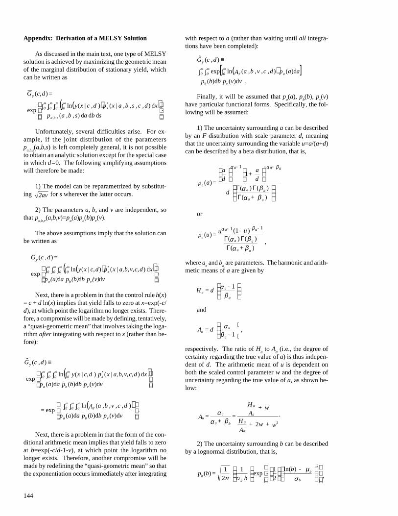
144

Appendix: Derivation of a MELSY Solution

As discussed in the main text, one type of MELSYsolution is achieved by maximizing the geometric meanof the marginal distribution of stationary yield, whichcan be written as

( )( )

∫∫∫∫ ∞∞∞∞

s b a s ,b ,ap

x d ,c , s ,b ,a|xp d ,c|xy

= d c,G

sba

x0000

y

ddd)(

d)()(lnexp

)(

,,

*

.

Unfortunately, several difficulties arise. For ex-ample, if the joint distribution of the parametersp

a,b,s(a,b,s) is left completely general, it is not possible

to obtain an analytic solution except for the special casein which d=0. The following simplifying assumptionswill therefore be made:

1) The model can be reparametrized by substitut-ing 2av for s wherever the latter occurs.

2) The parameters a, b, and v are independent, sothat p

a,b,v(a,b,v)=p

a(a)p

b(b)p

v(v).

The above assumptions imply that the solution canbe written as

( )( )

∫∫∫∫ ∞∞∞∞

v(v)p b(b)p a(a)p

xd c, v, b, a,|xpd c,|xy

=d ,cG

vba

x0000

y

ddd

d )()(lnexp

)(

*

.

Next, there is a problem in that the control rule h(x)= c + d ln(x) implies that yield falls to zero at x=exp(-c/d), at which point the logarithm no longer exists. There-fore, a compromise will be made by defining, tentatively,a “quasi-geometric mean” that involves taking the loga-rithm after integrating with respect to x (rather than be-fore):

( )

( ).

vvp bbp aap

d ,c ,v ,b ,aA =

vvp bbp aap

x d c, v, b, a,|xp d c,|xy

d ,cG

vba

y000

vba

x0000

y

∫∫∫

∫∫∫∫

≡

∞∞∞

∞∞∞∞

)d()d()d(

)(lnexp

)d()d()d(

d)()(lnexp

)(ˆ

*

Next, there is a problem in that the form of the con-ditional arithmetic mean implies that yield falls to zeroat b=exp(-c/d-1-v), at which point the logarithm nolonger exists. Therefore, another compromise will bemade by redefining the “quasi-geometric mean” so thatthe exponentiation occurs immediately after integrating

with respect to a (rather than waiting until all integra-tions have been completed):

( )[ ]. vvp bbp

aap d ,c ,v ,b ,aA

d ,cG

vb

ay000

y

)d()d(

)d()(lnexp

)(ˆ

∫∫∫

≡∞∞∞

Finally, it will be assumed that pa(a), p

b(b), p

v(v)

have particular functional forms. Specifically, the fol-lowing will be assumed:

1) The uncertainty surrounding a can be describedby an F distribution with scale parameter d, meaningthat the uncertainty surrounding the variable u=a/(a+d)can be described by a beta distribution, that is,

Γ

ΓΓ

+

d

d

a +

d

a

= ap

aa

aaa

aaa - - -

)(

)()(

1)(

1

βαβα

βαα

or

)(

)()()(1

)(1 1

+

u - u = up

aa

aa

u

- - aa

βαβα

βα

ΓΓΓ ,

where aa and b

a are parameters. The harmonic and arith-

metic means of a are given by

- d = H

a

aa β

α 1

and

-

d =Aa

aa

1 β

α ,

respectively. The ratio of Ha to A

a (i.e., the degree of

certainty regarding the true value of a) is thus indepen-dent of d. The arithmetic mean of u is dependent onboth the scaled control parameter w and the degree ofuncertainty regarding the true value of a, as shown be-low:

w + w + A

H

w+ A

H

= +

= A

a

a

a

a

ba

au

22βαα .

2) The uncertainty surrounding b can be describedby a lognormal distribution, that is,

- b

- b

= bpb

b

bb

σ

µσπ

)(ln

2

1exp

1

2

1)(

2

,

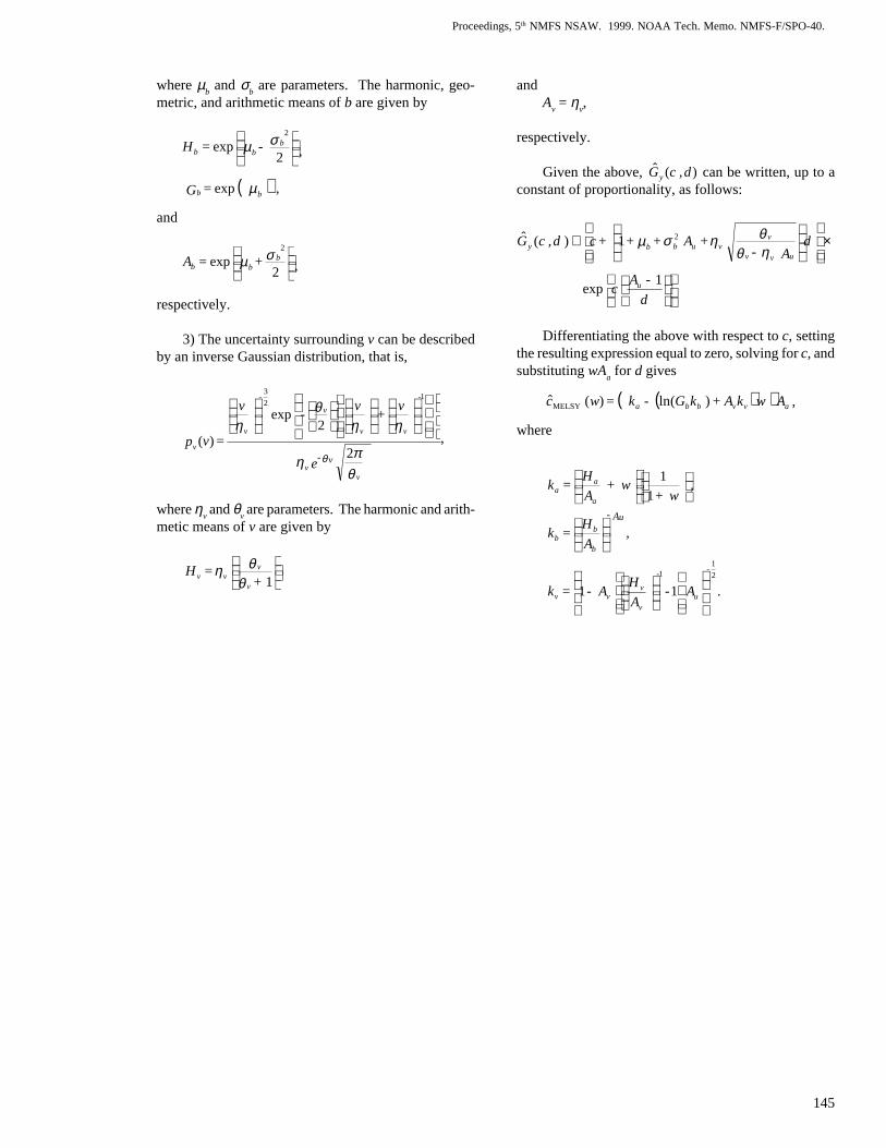
145


where µb and σ

b are parameters. The harmonic, geo-

metric, and arithmetic means of b are given by

2

exp2σµ b

bb - = H ,

( ) , = G bb µexp

and

+ = A bbb

2

exp2

σµ ,

respectively.

3) The uncertainty surrounding v can be describedby an inverse Gaussian distribution, that is,

e

v

+ v

- v

= vp

vv

v

-

v

v

v

v

v -

θπη

ηηθ

η

θ 2

2exp

)(

12

3 -

,

where ηv and θ

v are parameters. The harmonic and arith-

metic means of v are given by

1 +

= Hv

vvv θ

θη

andA

v = η

v,

respectively.

Given the above, )(ˆ d ,cGy can be written, up to aconstant of proportionality, as follows:

d

- A c

dA -

+ A + + + c d ,cG

u

uvv

vvubby

×

∝

1exp

1)(ˆ 2

ηθθησµ

Differentiating the above with respect to c, settingthe resulting expression equal to zero, solving for c, andsubstituting wA

a for d gives

( )( ) avvbba A wkA +kG - k = w c ) (ln)(ˆMELSY ,

where

.A - A

H A - = k

,A

H = k

, w+

w+ A

H = k

uv

v

-

vv

b

bb

a

aa

A - u

11

1

1

1 2

1 -

Documents

Optimizing Harvest Control Rules In the Presence of