OTDR VISA - xbest.pl - fibre optic cables & accessories€¦ · · 2011-10-12OTDR VISA . OPTICAL REFLECTOMETER (OTDR) OPTICAL POWER METER . ... Principle of instrument operation

OTDR VISA

OPTICAL REFLECTOMETER (OTDR)

OPTICAL POWER METER

User’s Guide

© 2011

2

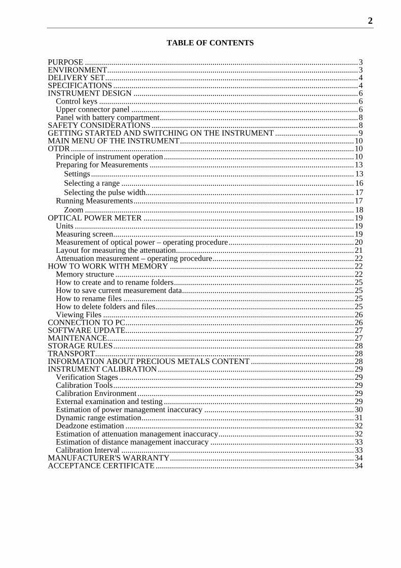
TABLE OF CONTENTS

PURPOSE .......................................................................................................................................3 ENVIRONMENT............................................................................................................................3 DELIVERY SET.............................................................................................................................4 SPECIFICATIONS .........................................................................................................................4 INSTRUMENT DESIGN ...............................................................................................................6

Control keys ................................................................................................................................6 Upper connector panel ................................................................................................................6 Panel with battery compartment..................................................................................................8

SAFETY CONSIDERATIONS ......................................................................................................8 GETTING STARTED AND SWITCHING ON THE INSTRUMENT .........................................9 MAIN MENU OF THE INSTRUMENT......................................................................................10 OTDR............................................................................................................................................10

Principle of instrument operation..............................................................................................10 Preparing for Measurements .....................................................................................................13

Settings .................................................................................................................................. 13 Selecting a range ................................................................................................................... 16 Selecting the pulse width....................................................................................................... 17

Running Measurements.............................................................................................................17 Zoom ..................................................................................................................................... 18

OPTICAL POWER METER ........................................................................................................19 Units ..........................................................................................................................................19 Measuring screen.......................................................................................................................19 Measurement of optical power – operating procedure..............................................................20 Layout for measuring the attenuation........................................................................................21 Attenuation measurement – operating procedure......................................................................22

HOW TO WORK WITH MEMORY ...........................................................................................22 Memory structure ......................................................................................................................22 How to create and to rename folders.........................................................................................25 How to save current measurement data.....................................................................................25 How to rename files ..................................................................................................................25 How to delete folders and files..................................................................................................25 Viewing Files ............................................................................................................................26

CONNECTION TO PC.................................................................................................................26 SOFTWARE UPDATE.................................................................................................................27 MAINTENANCE..........................................................................................................................27 STORAGE RULES.......................................................................................................................28 TRANSPORT................................................................................................................................28 INFORMATION ABOUT PRECIOUS METALS CONTENT ...................................................28 INSTRUMENT CALIBRATION.................................................................................................29

Verification Stages ....................................................................................................................29 Calibration Tools.......................................................................................................................29 Calibration Environment ...........................................................................................................29 External examination and testing ..............................................................................................29 Estimation of power management inaccuracy ..........................................................................30 Dynamic range estimation.........................................................................................................31 Deadzone estimation .................................................................................................................32 Estimation of attenuation management inaccuracy...................................................................32 Estimation of distance management inaccuracy .......................................................................33 Calibration Interval ...................................................................................................................33

MANUFACTURER'S WARRANTY...........................................................................................34 ACCEPTANCE CERTIFICATE ..................................................................................................34

3

PURPOSE

OTDR VISA is an optical reflectometer (hereinafter OTDR) for two wavelengths: 1310 and 1550 nm.

As additional options can be installed:

an optical power meter of the radiation with wavelengths: 1310 / 1550 nm;

a laser light source at a wavelength of 650 nm for visual detection of optical fiber (OF) damage.

Certificate of measuring device type approval No 42479. Public register RF No. ГР 46680-11.

The instrument makes it possible:

to determine the distribution of losses along the fiber-optic communication line (FOCL), to identify defective parts or elements of the communication line,

to determine the exact location of the breaks or damaged spans of the FOCL,

to estimate total losses in a fiber-optic communication line by the acceptance of the line and by periodic testing,

to measure the average losses of optical fiber on spools, the uniformity of losses distribution in the fiber and to detect the presence of local defects in fiber production,

to measure the losses in mechanical and welded joints,

to detect gradual or sudden deterioration of fiber quality by comparing its performance with earlier measurements,

to measure the average optical power (in units of dBm and mW) when operating with an external laser light source at wavelengths of 1310 nm and 1550 nm,

to store measurements (OTDR measurements and power measurements) in nonvolatile memory with the possibility of their review or subsequent transfer to a PC.

Range of application of the instrument OTDR VISA - manufacture of optical fiber and cable, construction of a fiber-optic communication lines (FOCL), diagnostics and maintenance of the status of fibers, cables and fiber-optic communication lines.

ENVIRONMENT

Ambient air temperature from plus 5 C to plus 50 С; Relative air humidity max. 90 % by 25 С; Atmospheric pressure from 86 to 106,7 kPa.

4

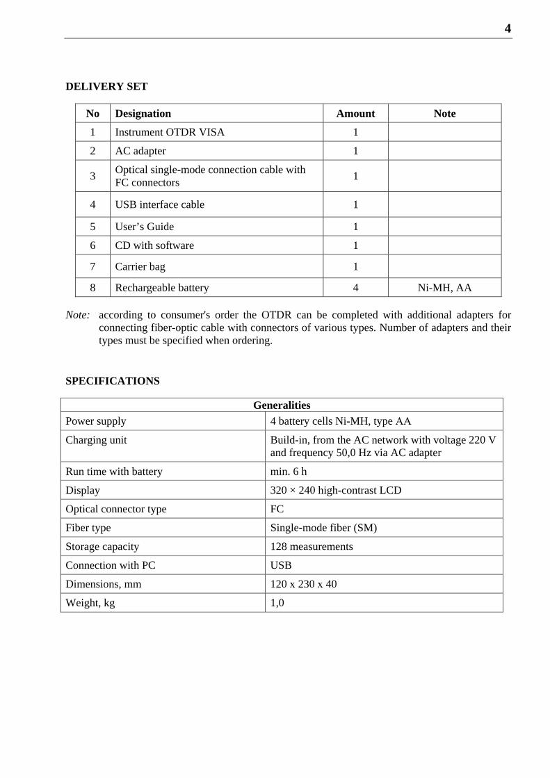
DELIVERY SET

No Designation Amount Note

1 Instrument OTDR VISA 1

2 AC adapter 1

3 Optical single-mode connection cable with FC connectors

1

4 USB interface cable 1

5 User’s Guide 1

6 CD with software 1

7 Carrier bag 1

8 Rechargeable battery 4 Ni-MH, AA

Note: according to consumer's order the OTDR can be completed with additional adapters for connecting fiber-optic cable with connectors of various types. Number of adapters and their types must be specified when ordering.

SPECIFICATIONS

Generalities

Power supply 4 battery cells Ni-MH, type АА

Charging unit Build-in, from the AC network with voltage 220 V and frequency 50,0 Hz via AC adapter

Run time with battery min. 6 h

Display 320 × 240 high-contrast LCD

Optical connector type FC

Fiber type Single-mode fiber (SM)

Storage capacity 128 measurements

Connection with PC USB

Dimensions, mm 120 х 230 х 40

Weight, kg 1,0

5

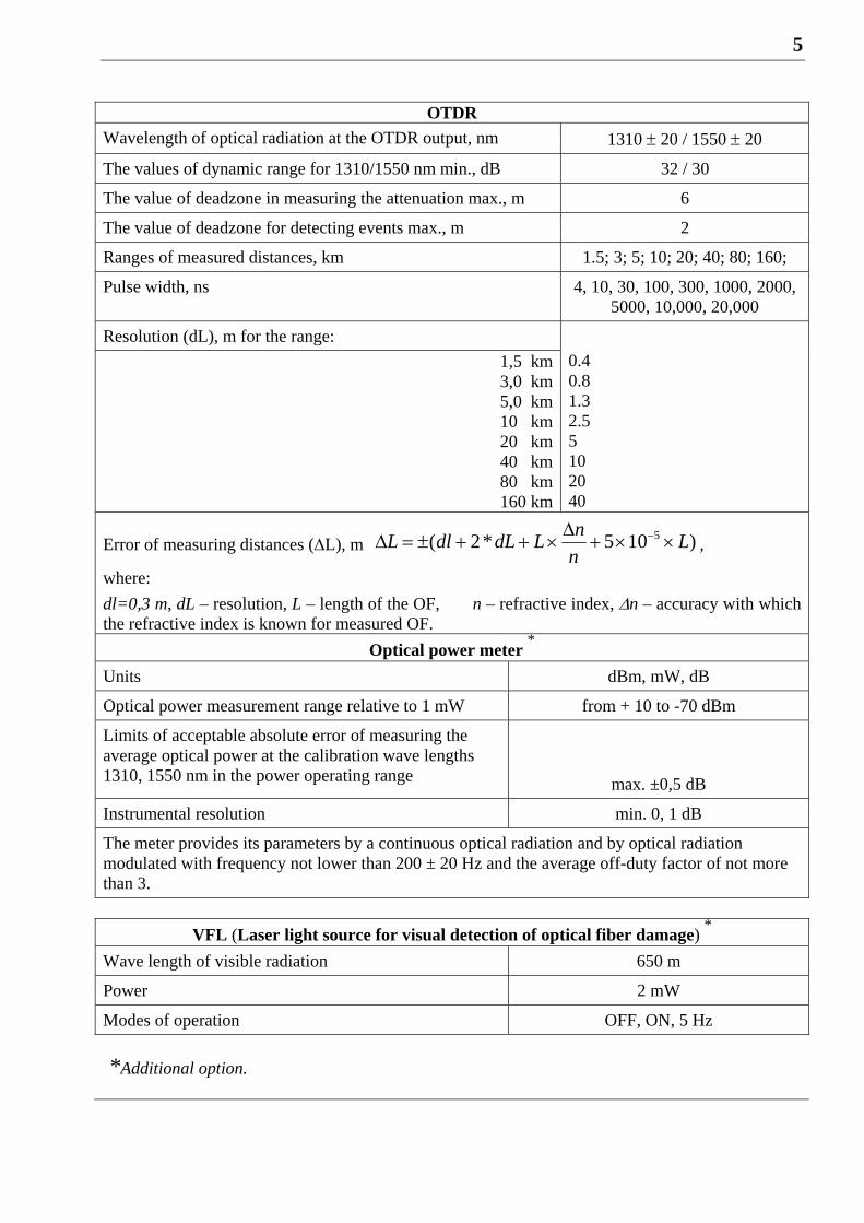
OTDR

Wavelength of optical radiation at the OTDR output, nm 1310 20 / 1550 20

The values of dynamic range for 1310/1550 nm min., dB 32 / 30

The value of deadzone in measuring the attenuation max., m 6

The value of deadzone for detecting events max., m 2

Ranges of measured distances, km 1.5; 3; 5; 10; 20; 40; 80; 160;

Pulse width, ns 4, 10, 30, 100, 300, 1000, 2000, 5000, 10,000, 20,000

Resolution (dL), m for the range:

1,5 km3,0 km5,0 km10 km20 km40 km80 km160 km

0.4 0.8 1.3 2.5 5 10 20 40

Error of measuring distances (L), m )105*2( 5 Ln

nLdLdlL

,

where:

dl=0,3 m, dL – resolution, L – length of the OF, n – refractive index, n – accuracy with which the refractive index is known for measured OF.

Optical power meter *

Units dBm, mW, dB

Optical power measurement range relative to 1 mW from + 10 to -70 dBm

Limits of acceptable absolute error of measuring the average optical power at the calibration wave lengths 1310, 1550 nm in the power operating range

max. ±0,5 dB

Instrumental resolution min. 0, 1 dB

The meter provides its parameters by a continuous optical radiation and by optical radiation modulated with frequency not lower than 200 ± 20 Hz and the average off-duty factor of not more than 3.

VFL (Laser light source for visual detection of optical fiber damage) *

Wave length of visible radiation 650 m

Power 2 mW

Modes of operation OFF, ON, 5 Hz

*Additional option.

6

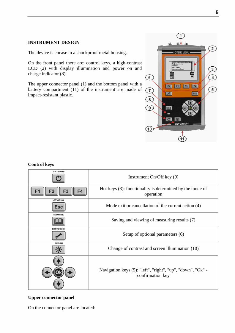
INSTRUMENT DESIGN

The device is encase in a shockproof metal housing.

On the front panel there are: control keys, a high-contrast LCD (2) with display illumination and power on and charge indicator (8).

The upper connector panel (1) and the bottom panel with a battery compartment (11) of the instrument are made of impact-resistant plastic.

Control keys

Instrument On/Off key (9)

Hot keys (3): functionality is determined by the mode of

operation

Mode exit or cancellation of the current action (4)

Saving and viewing of measuring results (7)

Setup of optional parameters (6)

Change of contrast and screen illumination (10)

Navigation keys (5): "left", "right", "up", "down", "Ok" - confirmation key

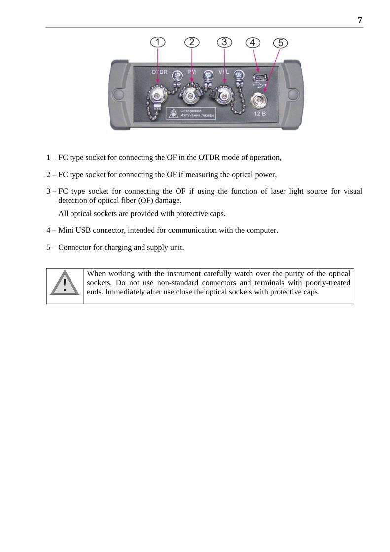
Upper connector panel

On the connector panel are located:

7

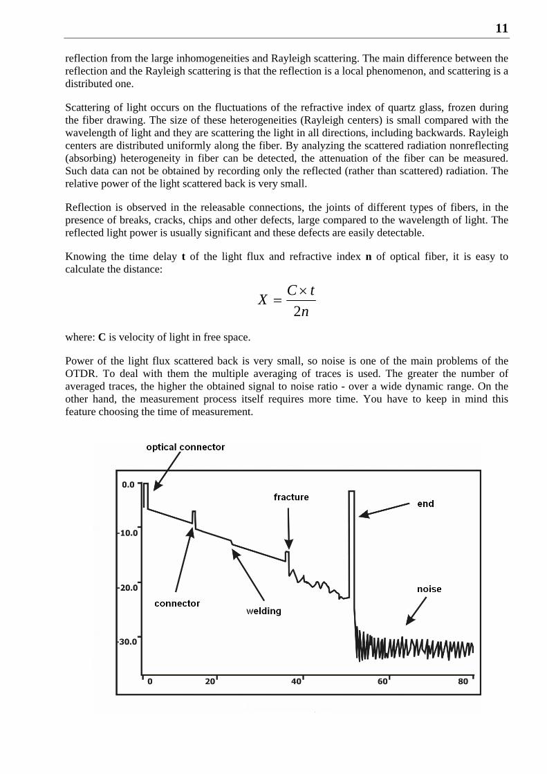
1 – FC type socket for connecting the OF in the OTDR mode of operation,

2 – FC type socket for connecting the OF if measuring the optical power,

3 – FC type socket for connecting the OF if using the function of laser light source for visual detection of optical fiber (OF) damage.

All optical sockets are provided with protective caps.

4 – Mini USB connector, intended for communication with the computer.

5 – Connector for charging and supply unit.

When working with the instrument carefully watch over the purity of the optical sockets. Do not use non-standard connectors and terminals with poorly-treated ends. Immediately after use close the optical sockets with protective caps.

8

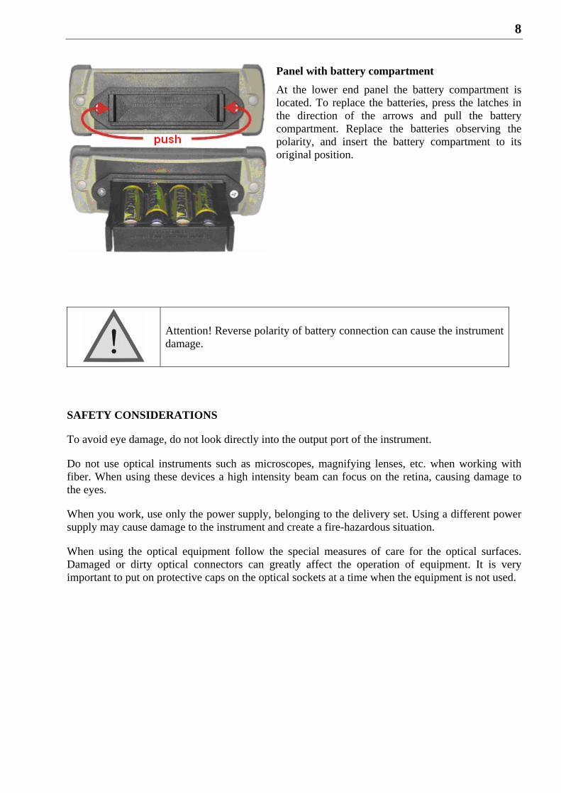
Panel with battery compartment

At the lower end panel the battery compartment is located. To replace the batteries, press the latches in the direction of the arrows and pull the battery compartment. Replace the batteries observing the polarity, and insert the battery compartment to its original position.

Attention! Reverse polarity of battery connection can cause the instrument damage.

SAFETY CONSIDERATIONS

To avoid eye damage, do not look directly into the output port of the instrument.

Do not use optical instruments such as microscopes, magnifying lenses, etc. when working with fiber. When using these devices a high intensity beam can focus on the retina, causing damage to the eyes.

When you work, use only the power supply, belonging to the delivery set. Using a different power supply may cause damage to the instrument and create a fire-hazardous situation.

When using the optical equipment follow the special measures of care for the optical surfaces. Damaged or dirty optical connectors can greatly affect the operation of equipment. It is very important to put on protective caps on the optical sockets at a time when the equipment is not used.

9

GETTING STARTED AND SWITCHING ON THE INSTRUMENT

Perform an external inspection of the instrument. Make sure there are no mechanical damages to the housing and the elements located on the front panel. If the instrument is kept at high humidity or low temperatures, allow it to dry for 24 hours under normal conditions.

Switch the instrument on pressing the "Instrument On/Off key". If the device is working properly and the battery is charged the following static picture appears on the screen:

To protect against accidental activation, after appearing the static picture within 3 seconds, press the "Ok", confirming the switching on.

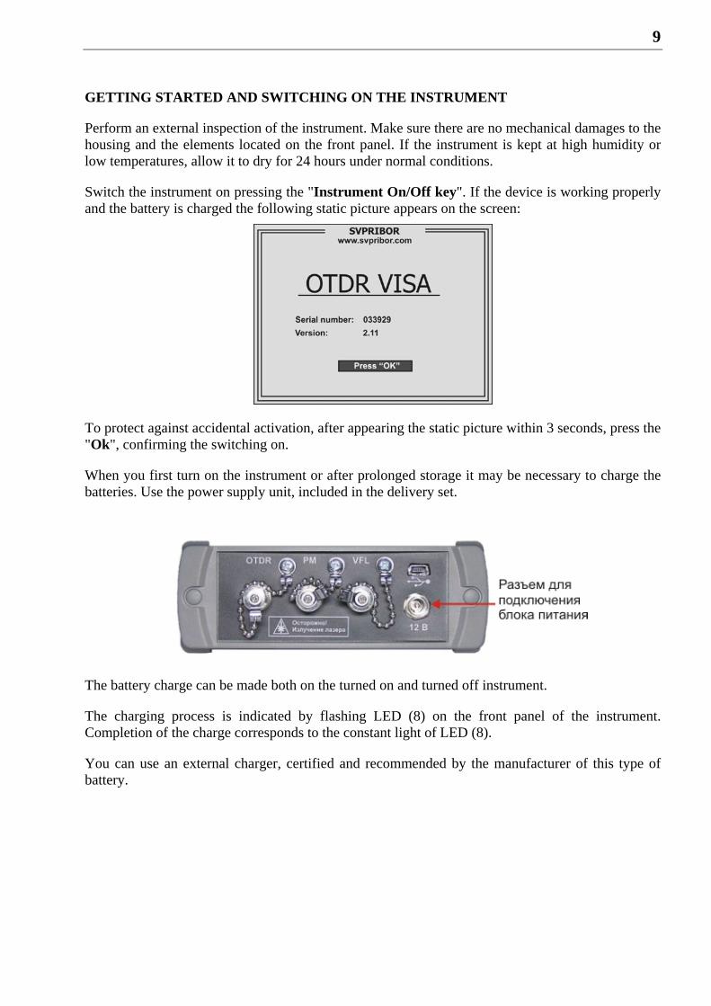
When you first turn on the instrument or after prolonged storage it may be necessary to charge the batteries. Use the power supply unit, included in the delivery set.

The battery charge can be made both on the turned on and turned off instrument.

The charging process is indicated by flashing LED (8) on the front panel of the instrument. Completion of the charge corresponds to the constant light of LED (8).

You can use an external charger, certified and recommended by the manufacturer of this type of battery.

10

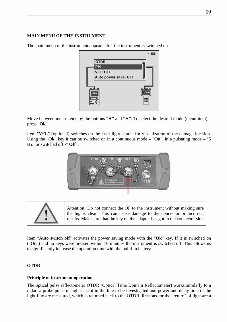
MAIN MENU OF THE INSTRUMENT

The main menu of the instrument appears after the instrument is switched on

Move between menu items by the buttons “” and “”. To select the desired mode (menu item) – press "Ok".

Item "VFL" (optional) switches on the laser light source for visualization of the damage location. Using the "Ok" key it can be switched on in a continuous mode – "On", in a pulsating mode – "5 Hz" or switched off -" Off".

Attention! Do not connect the OF to the instrument without making sure the lug is clean. This can cause damage to the connector or incorrect results. Make sure that the key on the adapter has got in the connector slot.

Item "Auto switch off" activates the power saving mode with the "Ok" key. If it is switched on ("On") and no keys were pressed within 10 minutes the instrument is switched off. This allows us to significantly increase the operation time with the build-in battery.

OTDR

Principle of instrument operation

The optical pulse reflectometer OTDR (Optical Time Domain Reflectometer) works similarly to a radar: a probe pulse of light is sent in the line to be investigated and power and delay time of the light flux are measured, which is returned back to the OTDR. Reasons for the "return" of light are a

11

reflection from the large inhomogeneities and Rayleigh scattering. The main difference between the reflection and the Rayleigh scattering is that the reflection is a local phenomenon, and scattering is a distributed one.

Scattering of light occurs on the fluctuations of the refractive index of quartz glass, frozen during the fiber drawing. The size of these heterogeneities (Rayleigh centers) is small compared with the wavelength of light and they are scattering the light in all directions, including backwards. Rayleigh centers are distributed uniformly along the fiber. By analyzing the scattered radiation nonreflecting (absorbing) heterogeneity in fiber can be detected, the attenuation of the fiber can be measured. Such data can not be obtained by recording only the reflected (rather than scattered) radiation. The relative power of the light scattered back is very small.

Reflection is observed in the releasable connections, the joints of different types of fibers, in the presence of breaks, cracks, chips and other defects, large compared to the wavelength of light. The reflected light power is usually significant and these defects are easily detectable.

Knowing the time delay t of the light flux and refractive index n of optical fiber, it is easy to calculate the distance:

n

tCX

2

where: C is velocity of light in free space.

Power of the light flux scattered back is very small, so noise is one of the main problems of the OTDR. To deal with them the multiple averaging of traces is used. The greater the number of averaged traces, the higher the obtained signal to noise ratio - over a wide dynamic range. On the other hand, the measurement process itself requires more time. You have to keep in mind this feature choosing the time of measurement.

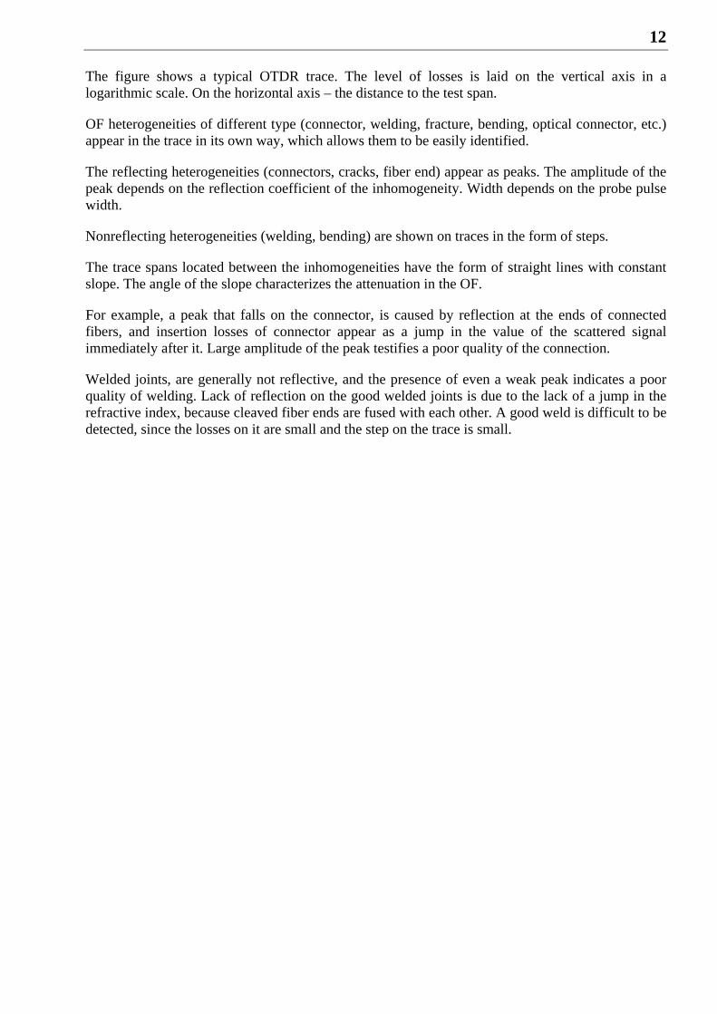
12

The figure shows a typical OTDR trace. The level of losses is laid on the vertical axis in a logarithmic scale. On the horizontal axis – the distance to the test span.

OF heterogeneities of different type (connector, welding, fracture, bending, optical connector, etc.) appear in the trace in its own way, which allows them to be easily identified.

The reflecting heterogeneities (connectors, cracks, fiber end) appear as peaks. The amplitude of the peak depends on the reflection coefficient of the inhomogeneity. Width depends on the probe pulse width.

Nonreflecting heterogeneities (welding, bending) are shown on traces in the form of steps.

The trace spans located between the inhomogeneities have the form of straight lines with constant slope. The angle of the slope characterizes the attenuation in the OF.

For example, a peak that falls on the connector, is caused by reflection at the ends of connected fibers, and insertion losses of connector appear as a jump in the value of the scattered signal immediately after it. Large amplitude of the peak testifies a poor quality of the connection.

Welded joints, are generally not reflective, and the presence of even a weak peak indicates a poor quality of welding. Lack of reflection on the good welded joints is due to the lack of a jump in the refractive index, because cleaved fiber ends are fused with each other. A good weld is difficult to be detected, since the losses on it are small and the step on the trace is small.

13

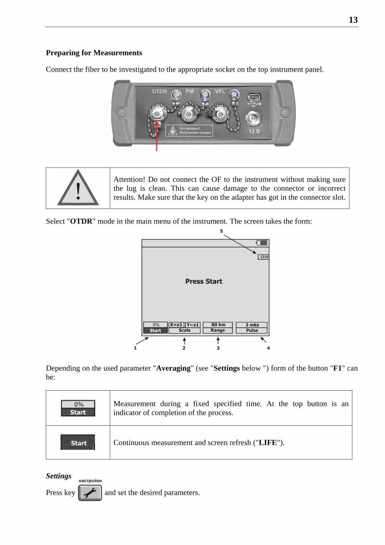
Preparing for Measurements

Connect the fiber to be investigated to the appropriate socket on the top instrument panel.


Select "OTDR" mode in the main menu of the instrument. The screen takes the form:

Depending on the used parameter "Averaging" (see "Settings below ") form of the button "F1" can be:

Measurement during a fixed specified time. At the top button is an indicator of completion of the process.

Continuous measurement and screen refresh ("LIFE").

Settings

Press key and set the desired parameters.

14

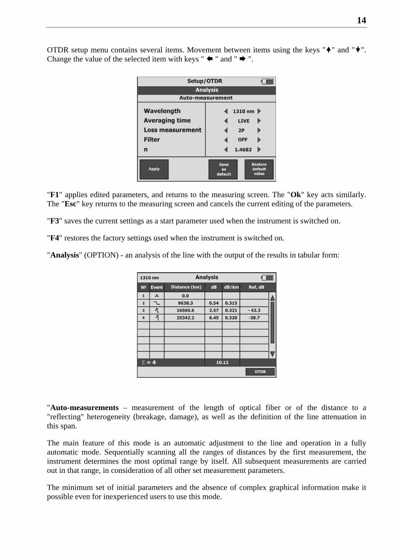
OTDR setup menu contains several items. Movement between items using the keys "" and "". Change the value of the selected item with keys " " and " ".

"F1" applies edited parameters, and returns to the measuring screen. The "Ok" key acts similarly. The "Esc" key returns to the measuring screen and cancels the current editing of the parameters.

"F3" saves the current settings as a start parameter used when the instrument is switched on.

"F4" restores the factory settings used when the instrument is switched on.

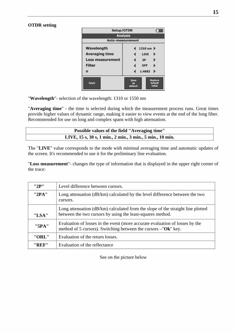
"Analysis" (OPTION) - an analysis of the line with the output of the results in tabular form:

"Auto-measurements – measurement of the length of optical fiber or of the distance to a "reflecting" heterogeneity (breakage, damage), as well as the definition of the line attenuation in this span.

The main feature of this mode is an automatic adjustment to the line and operation in a fully automatic mode. Sequentially scanning all the ranges of distances by the first measurement, the instrument determines the most optimal range by itself. All subsequent measurements are carried out in that range, in consideration of all other set measurement parameters.

The minimum set of initial parameters and the absence of complex graphical information make it possible even for inexperienced users to use this mode.

15

OTDR setting

"Wavelength"- selection of the wavelength: 1310 or 1550 nm

"Averaging time" - the time is selected during which the measurement process runs. Great times provide higher values of dynamic range, making it easier to view events at the end of the long fiber. Recommended for use on long and complex spans with high attenuation.

Possible values of the field "Averaging time" LIVE, 15 s, 30 s, 1 min., 2 min., 3 min., 5 min., 10 min.

The "LIVE" value corresponds to the mode with minimal averaging time and automatic updates of the screen. It's recommended to use it for the preliminary line evaluation.

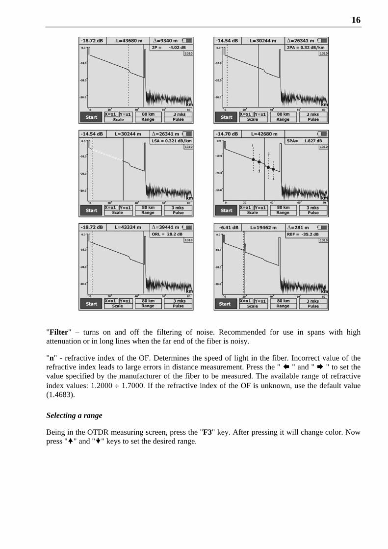
"Loss measurement"- changes the type of information that is displayed in the upper right corner of the trace:

"2P" Level difference between cursors.

"2PA" Long attenuation (dB/km) calculated by the level difference between the two cursors.

"LSA"

Long attenuation (dB/km) calculated from the slope of the straight line plotted between the two cursors by using the least-squares method.

"5PA" Evaluation of losses in the event (more accurate evaluation of losses by the method of 5 cursors). Switching between the cursors –"Ok" key.

"ORL" Evaluation of the return losses.

"REF" Evaluation of the reflectance

See on the picture below

16

"Filter" – turns on and off the filtering of noise. Recommended for use in spans with high attenuation or in long lines when the far end of the fiber is noisy.

"n" - refractive index of the OF. Determines the speed of light in the fiber. Incorrect value of the refractive index leads to large errors in distance measurement. Press the " " and " " to set the value specified by the manufacturer of the fiber to be measured. The available range of refractive index values: 1.2000 1.7000. If the refractive index of the OF is unknown, use the default value (1.4683).

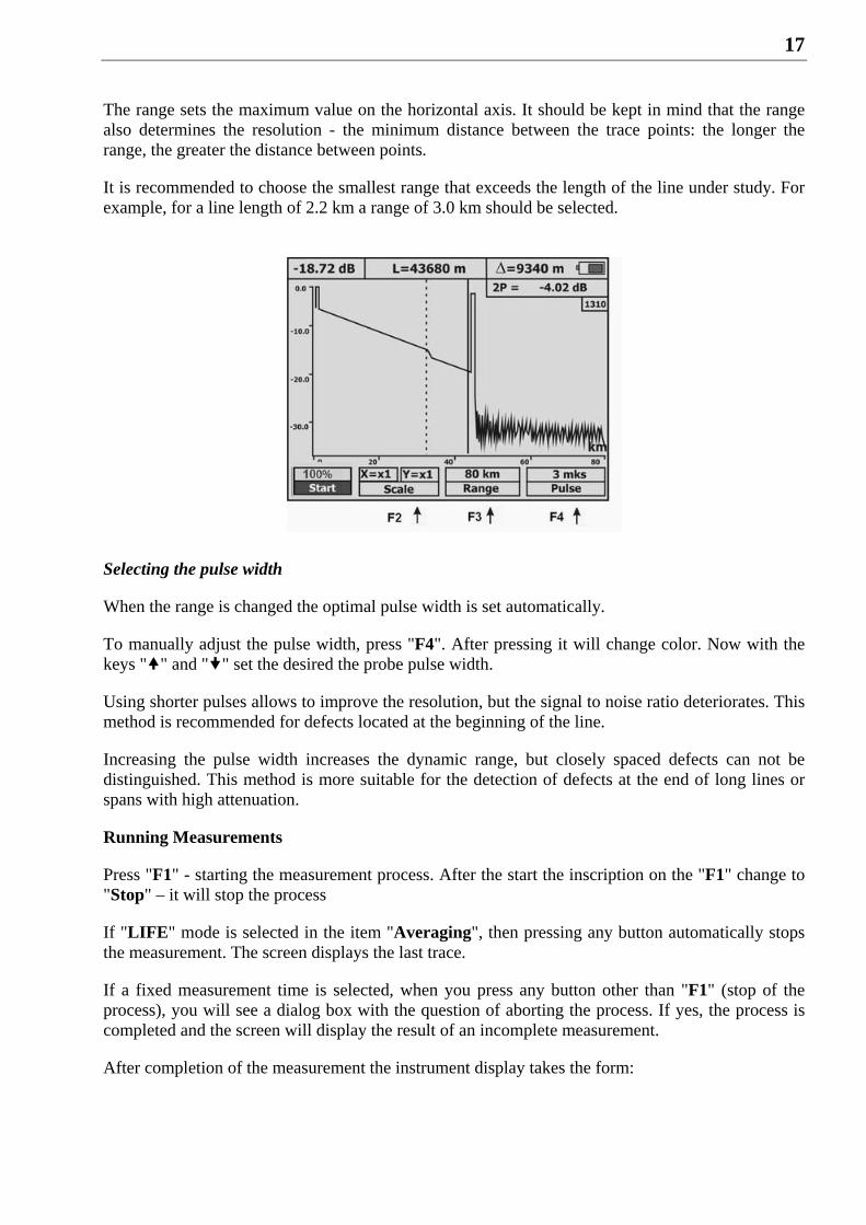
Selecting a range

Being in the OTDR measuring screen, press the "F3" key. After pressing it will change color. Now press "" and "" keys to set the desired range.

17

The range sets the maximum value on the horizontal axis. It should be kept in mind that the range also determines the resolution - the minimum distance between the trace points: the longer the range, the greater the distance between points.

It is recommended to choose the smallest range that exceeds the length of the line under study. For example, for a line length of 2.2 km a range of 3.0 km should be selected.

Selecting the pulse width

When the range is changed the optimal pulse width is set automatically.

To manually adjust the pulse width, press "F4". After pressing it will change color. Now with the keys "" and "" set the desired the probe pulse width.

Using shorter pulses allows to improve the resolution, but the signal to noise ratio deteriorates. This method is recommended for defects located at the beginning of the line.

Increasing the pulse width increases the dynamic range, but closely spaced defects can not be distinguished. This method is more suitable for the detection of defects at the end of long lines or spans with high attenuation.

Running Measurements

Press "F1" - starting the measurement process. After the start the inscription on the "F1" change to "Stop" – it will stop the process

If "LIFE" mode is selected in the item "Averaging", then pressing any button automatically stops the measurement. The screen displays the last trace.

If a fixed measurement time is selected, when you press any button other than "F1" (stop of the process), you will see a dialog box with the question of aborting the process. If yes, the process is completed and the screen will display the result of an incomplete measurement.

After completion of the measurement the instrument display takes the form:

18

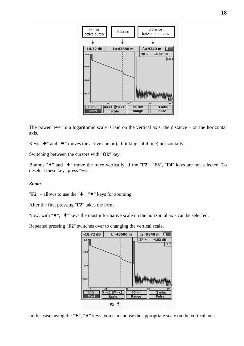
The power level in a logarithmic scale is laid on the vertical axis, the distance – on the horizontal axis.

Keys "" and "" moves the active cursor (a blinking solid line) horizontally.

Switching between the cursors with "Ok" key.

Buttons "" and "" move the trace vertically, if the "F2", "F3", "F4" keys are not selected. To deselect these keys press "Esc".

Zoom

"F2" – allows to use the "", "" keys for zooming.

After the first pressing "F2" takes the form.

Now, with "", "" keys the most informative scale on the horizontal axis can be selected.

Repeated pressing "F2" switches over to changing the vertical scale.

In this case, using the "", "" keys, you can choose the appropriate scale on the vertical axis.

19

OPTICAL POWER METER

Optical power meter can measure:

average optical power at wavelengths of 1310 nm and 1550 nm in the linear and logarithmic scale,

attenuation in the OF at wavelengths of 1310 and 1550 nm - using a remote light source.

Units

Units of measure optical power:

linear units– mW (milliwatt)

logarithmic units – dBm (decibel of power)

Power in dBm is a logarithmic ratio of P power relative to the reference power P0 of one milliwatt:

P(dBm) = 10 lg (P/P0).

Accordingly, the same power in dBm and in mW is expressed by the ratio:

P(dBm) = 10 lg P(mW).

Logarithmic units are suitable for simultaneous use of power and attenuation. Attenuation in decibels is the difference between power in dBm - reference P0 - at the input of optical path and the measured P at the outlet of the path: Attenuation (dB) = P0 - P (dBm).

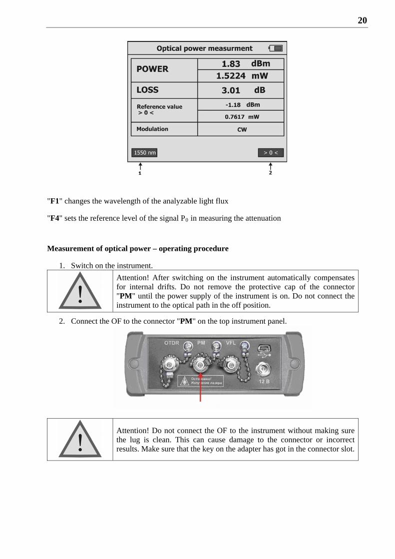
Measuring screen

In the "Power meter" mode the instrument carries out continuous measurements of average optical power and of attenuation with respect to the reference signal (see Fig.).

As auxiliary information the information about the magnitude of the reference signal level and its frequency (modulation line) is displayed. If the pulse-modulated signal is present on the input, then the magnitude of frequency modulation appears on the screen in the appropriate box. In the case of constant signal – "CW".

20

"F1" changes the wavelength of the analyzable light flux

"F4" sets the reference level of the signal P0 in measuring the attenuation

Measurement of optical power – operating procedure

1. Switch on the instrument.

Attention! After switching on the instrument automatically compensates for internal drifts. Do not remove the protective cap of the connector "PM" until the power supply of the instrument is on. Do not connect the instrument to the optical path in the off position.

2. Connect the OF to the connector "PM" on the top instrument panel.


21

3. In the main menu, select "Power Meter".

4. Using the "F1", select the desired wavelength.

Attention! If you select a wrong wavelength of the analyzable optical radiation, measurements will be incorrect.

5. Read optical power in the "Level" window.

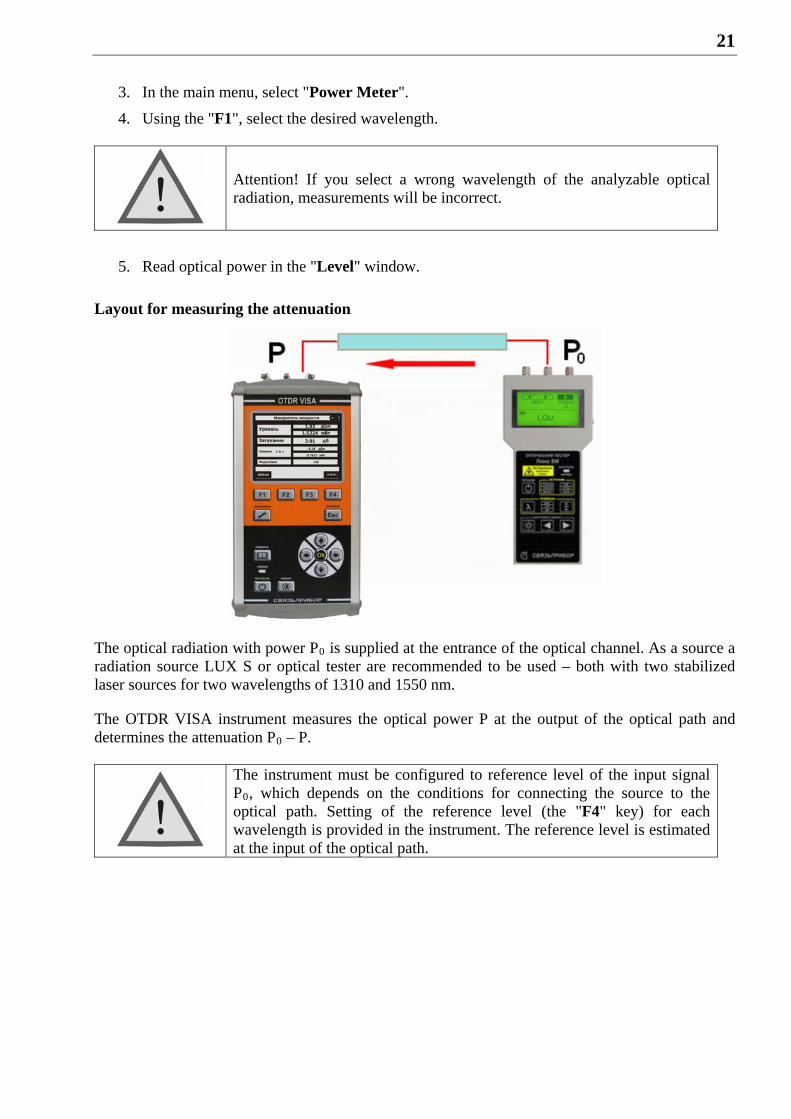
Layout for measuring the attenuation

The optical radiation with power P0 is supplied at the entrance of the optical channel. As a source a radiation source LUX S or optical tester are recommended to be used – both with two stabilized laser sources for two wavelengths of 1310 and 1550 nm.

The OTDR VISA instrument measures the optical power P at the output of the optical path and determines the attenuation P0 – P.

The instrument must be configured to reference level of the input signal P0, which depends on the conditions for connecting the source to the optical path. Setting of the reference level (the "F4" key) for each wavelength is provided in the instrument. The reference level is estimated at the input of the optical path.

22

Attenuation measurement – operating procedure

1. Switch to the power measurements mode. 2. At the input of the optical path the optical connecting cord of the source (to be connected to

the path input) first plug into a working power meter.

3. Select the desired wavelength using the "F1".

4. Wait till readings begin to be stable.

5. Press the "F4". The instrument is automatically configured to source level P0 and shows attenuation of 0.00 dB. The level of P0 and the wavelength are stored in nonvolatile memory of the instrument.

6. Connect the switched on instrument to the output of the optical path. If the reference level is adjusted for two wavelengths, then press "F1" to select the desired wavelength.

7. Measure the attenuation.

HOW TO WORK WITH MEMORY

Memory structure

In order to organize the results of measurements they are stored as files in specific folders.

Reflectometry results are saved in the BELLCORE SR-4731 format. This format allows:

to compare the results obtained with OTDRs from different manufacturers,

to save all the accumulated history of the fiber in an active base.

The files have the extension .sor and can be analyzed on a PC both using the standard software and using third-party applications.

The power measurement results are stored in the form of csv-files. On a PC, they are viewed using the standard software or any text editor.

To save the results of current measurements, or to view previously saved data, press the "memory" key.

If until this moment nothing has been stored, then the screen will display a list of available folders:

23

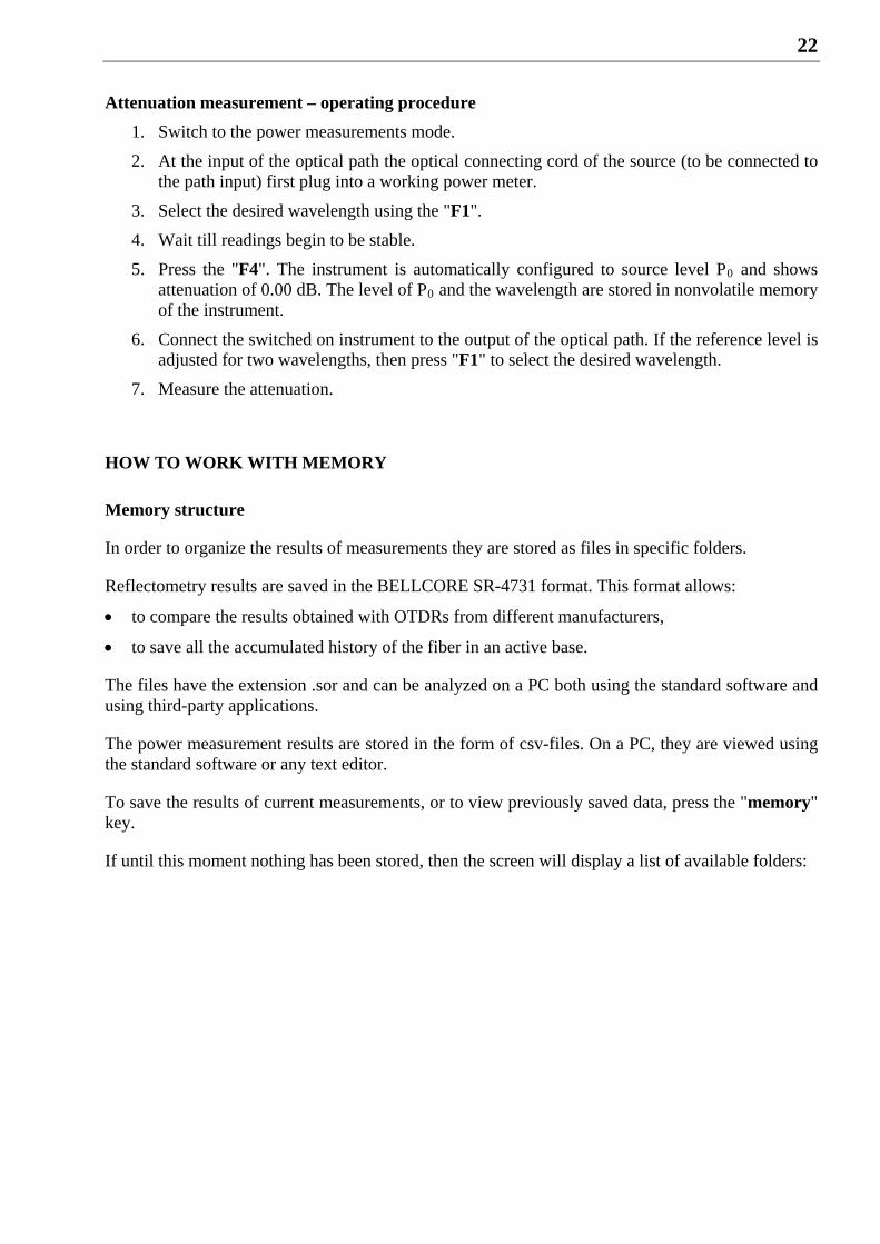
Navigating between folders is carried out with keys “” and “”. To enter the folder press "Ok". The "Esc" key returns to the current measurements.

"F1" allows to create a new folder. The results of the current measurements can only be saved in folders. Maximum number of folders - 32. The folder names of more than 8 characters are displayed on the screen of the instrument in an shortened format, with the addition of the symbol ~ and the order number. At the bottom of the screen an information line is located that contains the full name of the folder. Maximum number of characters in a name - 30. By default, there are two folders: "PM" and "OTDR". Properties of all the folders are identical.

"F2" allows to rename the selected folder.

"F3" deletes the selected folder.

"F4" - setting (correction) of the time and date for the current session of measurements. The instrument automatically stores the values of recent changes of these parameters and puts them by the next start. Count of the real-time occurs only during instrument operation.

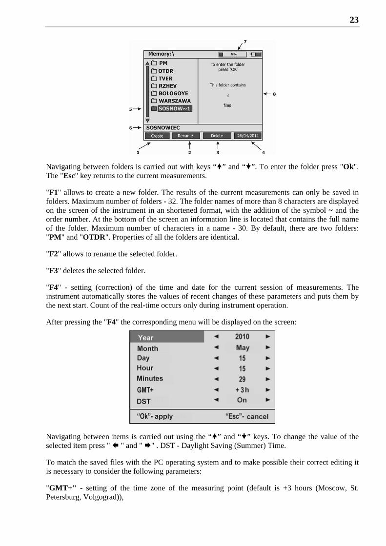
After pressing the "F4" the corresponding menu will be displayed on the screen:

Navigating between items is carried out using the “” and “” keys. To change the value of the selected item press " " and " " . DST - Daylight Saving (Summer) Time.

To match the saved files with the PC operating system and to make possible their correct editing it is necessary to consider the following parameters:

"GMT+" - setting of the time zone of the measuring point (default is +3 hours (Moscow, St. Petersburg, Volgograd)),

24

"OO/BB"- activation of an automatic changeover between winter and summer time.

"Ok" confirms the use of the edited parameters and returns to the measuring screen. "Esc" returns to the measuring screen and cancels the current editing of the parameters.

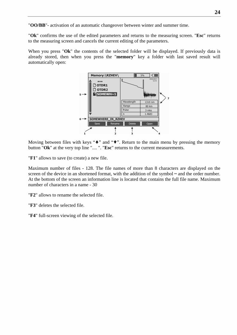
When you press "Ok" the contents of the selected folder will be displayed. If previously data is already stored, then when you press the "memory" key a folder with last saved result will automatically open:

Moving between files with keys “” and “”. Return to the main menu by pressing the memory button "Ok" at the very top line ".... ". "Esc" returns to the current measurements.

"F1" allows to save (to create) a new file.

Maximum number of files - 128. The file names of more than 8 characters are displayed on the screen of the device in an shortened format, with the addition of the symbol ~ and the order number. At the bottom of the screen an information line is located that contains the full file name. Maximum number of characters in a name - 30

"F2" allows to rename the selected file.

"F3" deletes the selected file.

"F4" full-screen viewing of the selected file.

25

How to create and to rename folders

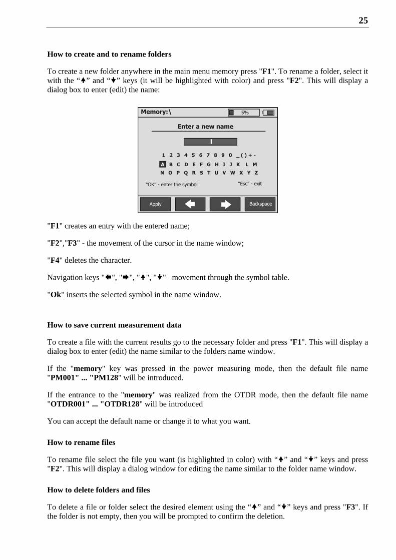
To create a new folder anywhere in the main menu memory press "F1". To rename a folder, select it with the “” and “” keys (it will be highlighted with color) and press "F2". This will display a dialog box to enter (edit) the name:

"F1" creates an entry with the entered name;

"F2","F3" - the movement of the cursor in the name window;

"F4" deletes the character.

Navigation keys "", "", "", ""– movement through the symbol table.

"Ok" inserts the selected symbol in the name window.

How to save current measurement data

To create a file with the current results go to the necessary folder and press "F1". This will display a dialog box to enter (edit) the name similar to the folders name window.

If the "memory" key was pressed in the power measuring mode, then the default file name "PM001" ... "PM128" will be introduced.

If the entrance to the "memory" was realized from the OTDR mode, then the default file name "OTDR001" ... "OTDR128" will be introduced

You can accept the default name or change it to what you want.

How to rename files

To rename file select the file you want (is highlighted in color) with “” and “” keys and press "F2". This will display a dialog window for editing the name similar to the folder name window.

How to delete folders and files

To delete a file or folder select the desired element using the “” and “” keys and press "F3". If the folder is not empty, then you will be prompted to confirm the deletion.

26

Viewing Files

To view select the desired file (is highlighted in color) using the “” and “” keys and press"F4". After that the full-screen mode will be entered with the stored measurement results.

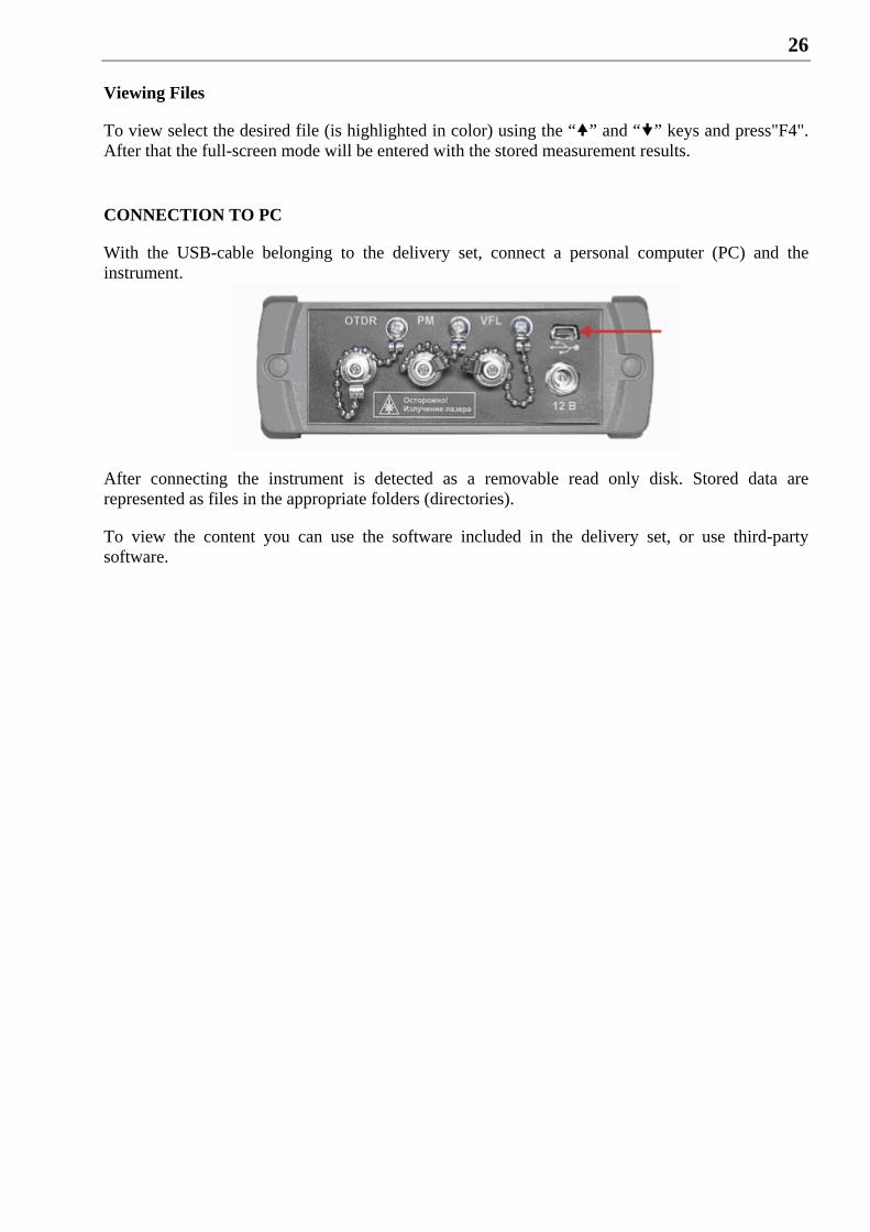
CONNECTION TO PC

With the USB-cable belonging to the delivery set, connect a personal computer (PC) and the instrument.

After connecting the instrument is detected as a removable read only disk. Stored data are represented as files in the appropriate folders (directories).

To view the content you can use the software included in the delivery set, or use third-party software.

27

SOFTWARE UPDATE

The instrument allows you to independently update the internal software.

Attention! Incorrect actions when updating software may cause damage to the instrument. While the process it is necessary to ensure undisturbed operation of the PC and of the instrument (fully charge the battery or connect the power adapter).

Turn on the instrument by holding pressed both the "Power" key and the "F2" key until the service menu is displayed.

Select the "Software update" and confirm your choice with the "Ok" key (to cancel press "Esc"). When you confirm you will move to the program update mode.

Only then connect the instrument to the PC via USB-cable, belonging to the delivery set.

PC will automatically detect the instrument as a removable disk and it will download the file with current software version.

Using PC delete the file with current software version.

Copy on its place the file with an updated software version.

Attention! It is forbidden to rename the software file

The copying process is displayed on the PC screen. After a successful copying the instrument will notify and offer to turn off the power. In case of failure, the instrument displays an error message and the update process must be repeated.

Turn off the instrument and disconnect the USB-cable.

The software upgrade process is completed.

MAINTENANCE

Maintenance includes control inspection, during which are verified:

completeness of the instrument;

absence of mechanical damage to the housing, front panel, connection elements.

28

When working with the instrument carefully watch over the purity of the optical connectors. Immediately after use, protect the adapters with protective caps. Clean the connectors as follows:

1. Make dense wick out of cloth, intended for use with optical connectors, for example Kimwipes, so that its thickness is slightly less than the inner diameter of the optical connector bush.

2. Moisten it with pure alcohol (isopropyl or ethyl alcohol).

3. Carefully and gently wipe the connector inside the bush. After wiping let alcohol dry inside the connector bush, then you can measure.

STORAGE RULES

Until commissioning the OTDR should be stored in a warehouse under the following conditions:

Ambient air temperature from 5 C to 50 С;

Relative air humidity up to 90 % by 25 С.

The repository should be free of dust, acid and alkali vapors, aggressive gases and other hazardous substance that cause corrosion.

To avoid damages during long-term storage remove the battery from the battery compartment.

TRANSPORT

Transportation of the OTDR must be carried out in closed vehicles of any kind (by rail, road and river (in holds) transport).

During transportation by air the OTDR must be placed in a heated sealed compartment.

The parameters of climatic impacts on the OTDR in packages during transportation should be the following:

ambient air temperature from minus 20 to plus 50 C,

relative air humidity not more than 98 % by 35 С.

If the instrument was transported at temperatures below 0 C, it must be kept under normal conditions for 2 hours.

INFORMATION ABOUT PRECIOUS METALS CONTENT

The instrument doesn't contain precious metals.

29

INSTRUMENT CALIBRATION

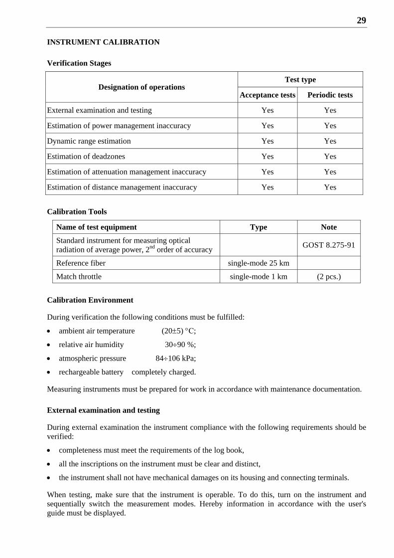
Verification Stages

Test type Designation of operations

Acceptance tests Periodic tests

External examination and testing Yes Yes

Estimation of power management inaccuracy Yes Yes

Dynamic range estimation Yes Yes

Estimation of deadzones Yes Yes

Estimation of attenuation management inaccuracy Yes Yes

Estimation of distance management inaccuracy Yes Yes

Calibration Tools

Name of test equipment Type Note

Standard instrument for measuring optical radiation of average power, 2nd order of accuracy

GOST 8.275-91

Reference fiber single-mode 25 km

Match throttle single-mode 1 km (2 pcs.)

Calibration Environment

During verification the following conditions must be fulfilled:

ambient air temperature (205) С;

relative air humidity 3090 %;

atmospheric pressure 84106 kPa;

rechargeable battery completely charged.

Measuring instruments must be prepared for work in accordance with maintenance documentation.

External examination and testing

During external examination the instrument compliance with the following requirements should be verified:

completeness must meet the requirements of the log book,

all the inscriptions on the instrument must be clear and distinct,

the instrument shall not have mechanical damages on its housing and connecting terminals.

When testing, make sure that the instrument is operable. To do this, turn on the instrument and sequentially switch the measurement modes. Hereby information in accordance with the user's guide must be displayed.

30

Attention!

The optical components of devices used for verification, must be cleaned of dust and wiped with a wad dipped in alcohol.

Estimation of power management inaccuracy

Verification operations to conform to the declared specifications are carried out according to the instruction MI 2505 - 98.

Here and below, the working standard for medium power of 2nd order of accuracy will be named in accordance with the measurement chain GOST 8.275-91 as standard instrument for measuring average power with 2nd order of accuracy (SI AP).

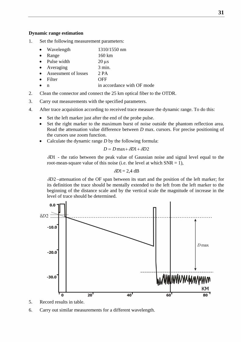
1. Assemble the facility shown in Figure

1. Stabilized radiation source 2. Optical attenuator 3. Standard wattmeter. 4. Instrument to be calibrated 5. Fiber-optic cable 6. SI AP, 2nd order of accuracy

2. Prepare instruments for work according to their operating manuals.

3. Set wavelength 1310 nm on all instruments.

4. Connect the output of optical attenuator 2 to the input of the standard wattmeter 3 and using the attenuator adjustment set its power output equal to the maximum power measured by the instrument to be calibrated.

5. Consistently carry out three power measurements with the standard wattmeter 3 and with the instrument to be calibrated 4.

6. Repeat the steps as claim 4, consistently reducing power (in increments of 5 ... 10 dB), reaching the minimum power, measurable with instrument to be calibrated.

7. Record results in table.

8. Repeat the measurement for wavelength 1550 nm.

31

Dynamic range estimation

1. Set the following measurement parameters:

Wavelength 1310/1550 nm Range 160 km Pulse width 20 s Averaging 3 min. Assessment of losses 2 PA Filter OFF n in accordance with OF mode

2. Clean the connector and connect the 25 km optical fiber to the OTDR.

3. Carry out measurements with the specified parameters.

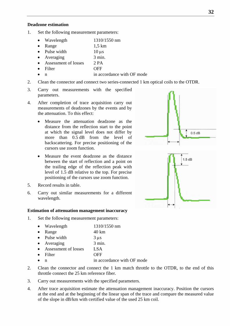
4. After trace acquisition according to received trace measure the dynamic range. To do this:

Set the left marker just after the end of the probe pulse. Set the right marker to the maximum burst of noise outside the phantom reflection area.

Read the attenuation value difference between D max. cursors. For precise positioning of the cursors use zoom function.

Calculate the dynamic range D by the following formula:

21max DDDD

1D - the ratio between the peak value of Gaussian noise and signal level equal to the root-mean-square value of this noise (i.e. the level at which SNR = 1),

1D = 2,4 dB

2D –attenuation of the OF span between its start and the position of the left marker; for its definition the trace should be mentally extended to the left from the left marker to the beginning of the distance scale and by the vertical scale the magnitude of increase in the level of trace should be determined.


6. Carry out similar measurements for a different wavelength.

32

Deadzone estimation


Wavelength 1310/1550 nm Range 1,5 km Pulse width 10 s Averaging 3 min. Assessment of losses 2 PA Filter OFF n in accordance with OF mode

2. Clean the connector and connect two series-connected 1 km optical coils to the OTDR.


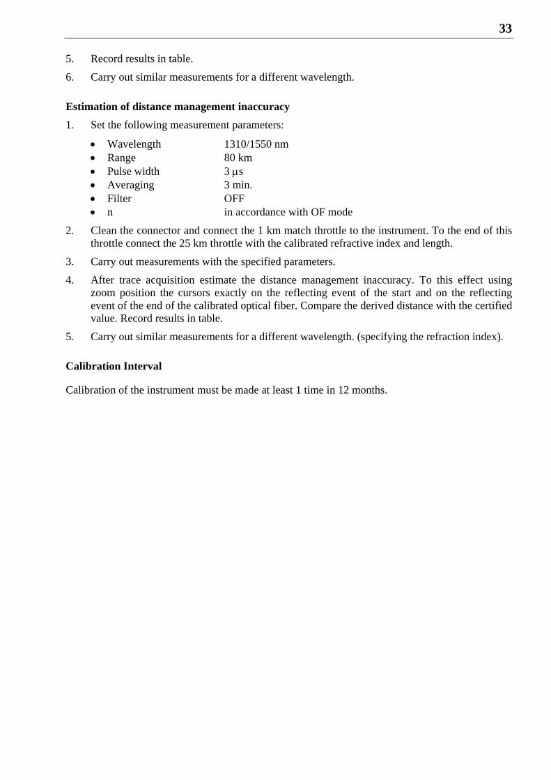
4. After completion of trace acquisition carry out measurements of deadzones by the events and by the attenuation. To this effect:

Measure the attenuation deadzone as the distance from the reflection start to the point at which the signal level does not differ by more than 0.5 dB from the level of backscattering. For precise positioning of the cursors use zoom function.

Measure the event deadzone as the distance between the start of reflection and a point on the trailing edge of the reflection peak with level of 1.5 dB relative to the top. For precise positioning of the cursors use zoom function.



Estimation of attenuation management inaccuracy


Wavelength 1310/1550 nm Range 40 km Pulse width 3 s Averaging 3 min. Assessment of losses LSA Filter OFF n in accordance with OF mode

2. Clean the connector and connect the 1 km match throttle to the OTDR, to the end of this throttle connect the 25 km reference fiber.


4. After trace acquisition estimate the attenuation management inaccuracy. Position the cursors at the end and at the beginning of the linear span of the trace and compare the measured value of the slope in dB/km with certified value of the used 25 km coil.

33



Estimation of distance management inaccuracy


Wavelength 1310/1550 nm Range 80 km Pulse width 3 s Averaging 3 min. Filter OFF n in accordance with OF mode

2. Clean the connector and connect the 1 km match throttle to the instrument. To the end of this throttle connect the 25 km throttle with the calibrated refractive index and length.


4. After trace acquisition estimate the distance management inaccuracy. To this effect using zoom position the cursors exactly on the reflecting event of the start and on the reflecting event of the end of the calibrated optical fiber. Compare the derived distance with the certified value. Record results in table.

5. Carry out similar measurements for a different wavelength. (specifying the refraction index).

Calibration Interval

Calibration of the instrument must be made at least 1 time in 12 months.

34

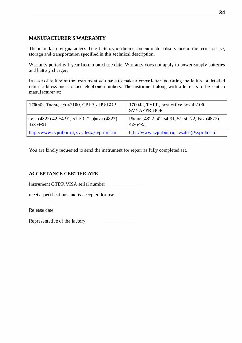
MANUFACTURER'S WARRANTY

The manufacturer guarantees the efficiency of the instrument under observance of the terms of use, storage and transportation specified in this technical description.

Warranty period is 1 year from a purchase date. Warranty does not apply to power supply batteries and battery charger.

In case of failure of the instrument you have to make a cover letter indicating the failure, a detailed return address and contact telephone numbers. The instrument along with a letter is to be sent to manufacturer at:

170043, Тверь, а/я 43100, СВЯЗЬПРИБОР 170043, TVER, post office box 43100 SVYAZPRIBOR

тел. (4822) 42-54-91, 51-50-72, факс (4822) 42-54-91

Phone (4822) 42-54-91, 51-50-72, Fax (4822) 42-54-91

http://www.svpribor.ru, [email protected] http://www.svpribor.ru, [email protected]

You are kindly requested to send the instrument for repair as fully completed set.

ACCEPTANCE CERTIFICATE

Instrument OTDR VISA serial number _______________

meets specifications and is accepted for use.

Release date __________________

Representative of the factory __________________

http://www.svpribor.ru/

mailto:[email protected]

http://www.svpribor.ru/

mailto:[email protected]

35

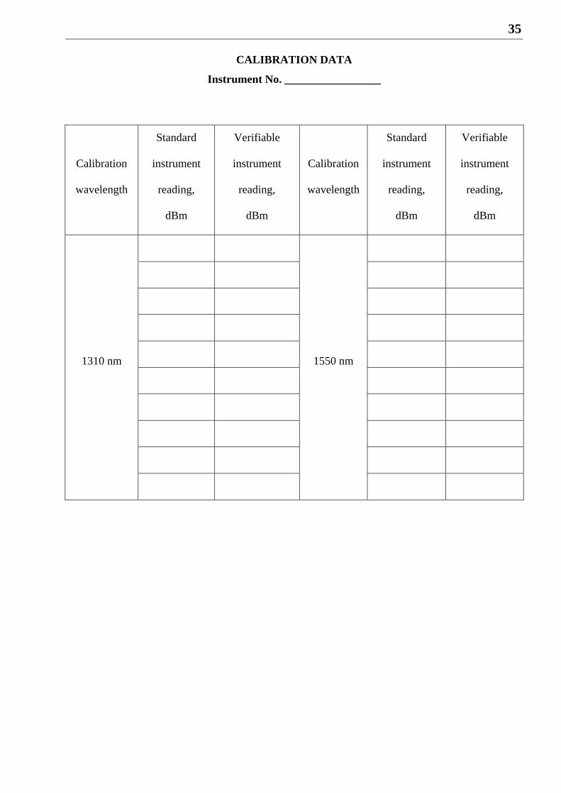
CALIBRATION DATA

Instrument No. _________________

Calibration

wavelength

Standard

instrument

reading,

dBm

Verifiable

instrument

reading,

dBm

Calibration

wavelength

Standard

instrument

reading,

dBm

Verifiable

instrument

reading,

dBm

1310 nm

1550 nm

36

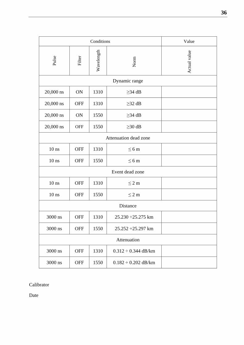
Conditions Value

Pul

se

Fil

ter

Wav

elen

gth

Nor

m

Act

ual v

alue

Dynamic range

20,000 ns ON 1310 ≥34 dB

20,000 ns OFF 1310 ≥32 dB

20,000 ns ON 1550 ≥34 dB

20,000 ns OFF 1550 ≥30 dB

Attenuation dead zone

10 ns OFF 1310 ≤ 6 m

10 ns OFF 1550 ≤ 6 m

Event dead zone

10 ns OFF 1310 ≤ 2 m

10 ns OFF 1550 ≤ 2 m

Distance

3000 ns OFF 1310 25.230 ÷25.275 km

3000 ns OFF 1550 25.252 ÷25.297 km

Attenuation

3000 ns OFF 1310 0.312 ÷ 0.344 dB/km

3000 ns OFF 1550 0.182 ÷ 0.202 dB/km

Calibrator

Date

Documents

OTDR VISA - xbest.pl - fibre optic cables & accessories€¦ · · 2011-10-12OTDR VISA . OPTICAL REFLECTOMETER (OTDR) OPTICAL POWER METER . ... Principle of instrument operation