Multiple Proxy Estimates of Atmospheric CO2 From an EarlyPaleocene RainforestJennifer B. Kowalczyk1,2 , Dana L. Royer1 , Ian M. Miller3, Clive W. Anderson4, David J. Beerling5,Peter J. Franks6, Michaela Grein7, Wilfried Konrad8, Anita Roth-Nebelsick9, Samuel A. Bowring10,Kirk R. Johnson11 , and Jahandar Ramezani10

1Department of Earth and Environmental Sciences, Wesleyan University, Middletown, CT, USA, 2Department of Earth,Environmental and Planetary Sciences, Brown University, Providence, RI, USA, 3Earth Sciences Department, DenverMuseum of Nature and Science, Denver, CO, USA, 4School of Mathematics and Statistics, University of Sheffield, Sheffield,UK, 5Department of Animal and Plant Sciences, University of Sheffield, Sheffield, UK, 6School of Life and EnvironmentalSciences, University of Sydney, Sydney, New South Wales, Australia, 7Übersee-Museum Bremen, Bremen, Germany,8Institute for Geosciences, University of Tübingen, Tübingen, Germany, 9State Museum of Natural History, Stuttgart,Germany, 10Department of Earth, Atmospheric and Planetary Sciences, Massachusetts Institute of Technology, Cambridge,MA, USA, 11National Museum of Natural History, Smithsonian Institution, Washington, DC, USA

Abstract Proxy estimates of atmospheric CO2 are necessary to reconstruct Earth’s climate history.Confidence in paleo-CO2 estimates can be increased by comparing results from multiple proxies at asingle site, but so far this strategy has been implemented only for marine-based techniques. Here we presentCO2 estimates for the well-studied early Paleocene Castle Rock site in Colorado using four paleobotanicalproxies. Median estimates range from 470 to 813 ppm, demonstrating fair correspondence. The synthesisyields a median of 616 ppm (352–1110 ppm at 95% confidence), considerably higher than previous earlyPaleocene CO2 estimates (~300 ppm). Ash bed geochronology by the high-precision U-Pbmethod places theCastle Rock assemblage at 63.844 ± 0.097 Ma (fully propagated 2σ error). When these results are placed intothe broader context of other Cenozoic CO2 estimates from plant-gas-exchange approaches and coevalestimates of global mean surface temperature, a pattern emerges of an Earth system sensitivity around 3 °Cper CO2 doubling during the Paleocene and Eocene, a time with little land ice, then steepening to>7 °C afterthe Eocene once land ice was present on Antarctica.

Plain Language Summary As atmospheric CO2 continues to increase, we enter a climate statewhose analog in terms of CO2 concentration is found millions of years ago. Information about climatefrom such distant times is only available to us via proxy methods (i.e., indicators of climate recorded inancient rocks and fossils); increasing confidence in proxy results is therefore a high priority. Here we comparefour different CO2 proxy methods using plant fossils from an exceptionally diverse rainforest that existed nearpresent-day Denver, Colorado, 63.8 million years ago. Estimates are largely congruent and higher thanpreviously thought (~600 ppm). The higher CO2 levels during this warm period are in better agreement withthe current understanding of long-term Earth system climate sensitivity, and results from the newergas-exchange proxy methods paint a coherent picture of Earth system sensitivity evolution over the Cenozoic.

1. Introduction

Long-term surface temperature is primarily controlled by the abundance of the greenhouse gas carbon diox-ide (Lacis et al., 2010). Atmospheric CO2 varied between ~180 to ~280 ppm over the past 800 kyr before theIndustrial Revolution (Luthi et al., 2008), but accelerating anthropogenic carbon emissions since then havepushed it to ~400 ppm. Projections show concentrations reaching >720 ppm by the end of the centuryunless emission rates are lowered (Intergovernmental Panel on Climate Change, 2014), a level perhaps notseen in over 30 million years (Beerling & Royer, 2011). To understand the response of climate to our currentincrease in atmospheric CO2 and to predict what climatic conditions future generations may face, reconstruc-tions of Earth’s pre-Pleistocene paleoclimate history—accessible only via proxy—are critical (Montañezet al., 2011).

Proxies for estimating a climate variable such as CO2 are based on responses of natural systems to the vari-able in a way that is preserved in the geologic record (Beerling & Royer, 2011). A compilation of CO2 estimates

KOWALCZYK ET AL. 1427

Paleoceanography and Paleoclimatology

RESEARCH ARTICLE10.1029/2018PA003356

Special Section:Climatic and Biotic Events ofthe Paleogene: Earth Systemsand Planetary Boundaries in aGreenhouse World

Key Points:• Multiproxy studies increase

confidence in paleoclimatereconstructions; we present the firstsuch study for land-based CO2

proxies• Our study highlights relatively new,

more widely applicable proxymethods based on robust models ofgas exchange in C3 photosynthesis

• Our CO2 estimates are morecongruent with the currentunderstanding of Earth systemsensitivity than are previous lowerestimates

Supporting Information:• Supporting Information S1• Data Set S1• Data Set S2• Data Set S3• Data Set S4• Data Set S5• Data Set S6• Data Set S7• Data Set S8• Data Set S9• Data Set S10• Data Set S11• Data Set S12• Data Set S13• Data Set S14

Correspondence to:J. B. Kowalczyk,jennifer_kowalczyk@brown.edu

Citation:Kowalczyk, J. B., Royer, D. L., Miller, I. M.,Anderson, C. W., Beerling, D. J., Franks,P. J., et al. (2018). Multiple proxy estimatesof atmospheric CO2 from an earlyPaleocene rainforest. Paleoceanographyand Paleoclimatology, 33, 1427–1438.https://doi.org/10.1029/2018PA003356

Received 4 MAR 2018Accepted 17 OCT 2018Accepted article online 24 OCT 2018Published online 21 DEC 2018

©2018. American Geophysical Union.All Rights Reserved.

over the Cenozoic from multiple methods shows considerable scatter (>2-fold) for most time intervals(Beerling & Royer, 2011). The best way to distinguish whether this scatter represents real, short-term CO2

variation or limitations of particular methods is to generate CO2 estimates from multiple methods at singlesites (Montañez et al., 2011).

Previous multiproxy studies have been limited to the marine alkenone and boron methods for the low-CO2 world (<400 ppm) of the Miocene (Badger et al., 2013) and Pliocene (Seki et al., 2010). Here weestimate CO2 for the exceptional early Paleocene fossil plant site Castle Rock (Ellis et al., 2003) with fourdifferent paleobotanical proxies. The Castle Rock section is located on the western edge of the DenverBasin in Colorado (Figure 1) with a direct radioisotopic age of 63.844 ± 0.060 Ma (±0.097 including allsources of uncertainty), ~2.2 (±0.06) Myr after the Cretaceous-Paleogene boundary (KPB) mass extinctionevent (see Text S1 for more information about the site and Text S3.11 for details of U-Pb isotopic analyses).Castle Rock contains the abundant remains of a rainforest preserved in situ over a short time period (<3 min stratigraphic section) by successive overbank flooding (Ellis et al., 2003). The species richness at CastleRock is several times higher than other post-KPB extinction sites in North America (Ellis et al., 2003;Johnson et al., 2003; Johnson & Ellis, 2002). The diversity of taxa, morphology of fossil leaves, and esti-mates of temperature and rainfall indicate that Castle Rock was similar to present-day tropical or para-tropical rainforests (Ellis et al., 2003). Despite being well studied, no estimates of atmospheric CO2 haveyet been published from the site.

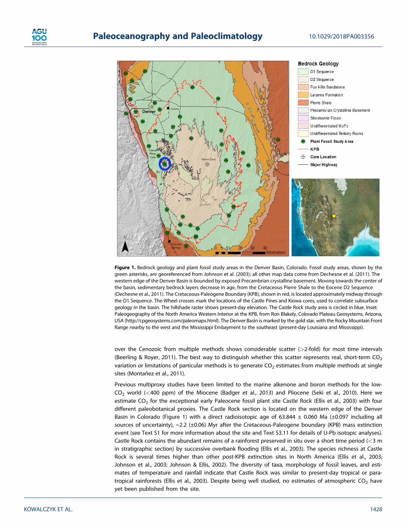
Figure 1. Bedrock geology and plant fossil study areas in the Denver Basin, Colorado. Fossil study areas, shown by thegreen asterisks, are georeferenced from Johnson et al. (2003); all other map data come from Dechesne et al. (2011). Thewestern edge of the Denver Basin is bounded by exposed Precambrian crystalline basement. Moving towards the center ofthe basin, sedimentary bedrock layers decrease in age, from the Cretaceous Pierre Shale to the Eocene D2 Sequence(Dechesne et al., 2011). The Cretaceous-Paleogene Boundary (KPB), shown in red, is located approximately midway throughthe D1 Sequence. The Wheel crosses mark the locations of the Castle Pines and Kiowa cores, used to correlate subsurfacegeology in the basin. The hillshade raster shows present-day elevation. The Castle Rock study area is circled in blue. Inset:Paleogeography of the North America Western Interior at the KPB, from Ron Blakely, Colorado Plateau Geosystems, Arizona,USA (http://cpgeosystems.com/paleomaps.html). The Denver Basin is marked by the gold star, with the Rocky Mountain FrontRange nearby to the west and the Mississippi Embayment to the southeast (present-day Louisiana and Mississippi).

10.1029/2018PA003356Paleoceanography and Paleoclimatology

KOWALCZYK ET AL. 1428

The four proxies applied here are the stomatal index (SI) and three newer methods based on C3 photosynth-esis: the BRYOCARB model for the astomatal nonvascular liverworts (Fletcher et al., 2006) and two others forstomatal-bearing plants, which we refer to here as the Franks (Franks et al., 2014) and Konrad (Konrad et al.,2008) models. The widely used (e.g., Barclay et al., 2010; Doria et al., 2011; Kürschner et al., 2008; Royer et al.,2001) SI method (Salisbury, 1927) derives from the inverse relation between atmospheric CO2 and the frac-tion of leaf epidermal cells that are stomata, the pores on the leaf surface that allow for gas exchange withthe atmosphere (Royer, 2001; Woodward, 1987). A drawback of this proxy is that the quantitative SI-CO2 rela-tionship is empirical and species-dependent, limiting its use to fossil taxa with very close living relatives(Beerling & Royer, 2002b; Royer, 2001). The newer, more complex gas-exchange models minimize this short-coming. Nonetheless, all of the described plant-based proxy methods have produced reliable estimates ofatmospheric CO2 concentration in different settings. Our goals here were (i) to estimate atmospheric CO2

concentration for the early Paleocene with greater confidence by applying multiple plant-based proxies toa single fossil site and (ii) to use this information to gain greater insight into long-term Earth systemclimate sensitivity.

2. Methods2.1. Proxy Models

The gas-exchange models (Franks, Konrad, and BRYOCARB) are based on a simple, well-validated model forC3 photosynthesis, where the rate of carbon assimilation is equal to the product of total leaf conductance toCO2 and the atmospheric-to-leaf-internal CO2 concentration gradient (Farquhar & Sharkey, 1982); we refer tothis as the Farquhar model. Additionally, in each of these models the carbon isotope discrimination duringphotosynthesis (Δ13C) is used to reconstruct the ratio of leaf-internal-to-atmospheric CO2 concentration(ci/ca). This fractionation, which occurs due to discrimination against 13C during CO2 diffusion into leaf (orthallose) intercellular spaces (4.4‰) and during carbon fixation by Rubisco (20–27‰), can be determinedfrom measurements of plant tissue carbon isotope composition (δ13C; corrected for diagenesis) and an esti-mate of paleo-atmospheric CO2 δ13C (corrected for soil respiration in the case of the BRYOCARB model).Although photorespiration may affect the relationship between leaf δ13C and ci/ca (Schubert & Jahren,2018), including this effect would increase our CO2 estimates from the Franks model by <50 ppm. A briefdescription of each gas-exchange model is given below; full details of these models and our methods aregiven in Texts S2 and S3.

For each proxy method, 95% confidence intervals for estimated CO2 were determined using 10,000 MonteCarlo simulations (Data Set S5) to propagate uncertainties in all input parameters.2.1.1. Franks ModelThe Franks model for stomatal-bearing vascular plants (Franks et al., 2014) consists of two main equationsthat are iteratively solved for two unknowns: paleo-photosynthetic rate and paleo-atmospheric CO2 concen-tration. Key input parameters come from stomatal morphology and carbon isotopic composition measure-ments on fossil leaf tissue and from gas-exchange measurements on present-day relatives. The first of theiteratively solved equations is the Farquhar model, where total leaf conductance to CO2 is determined largelyby stomatal density and morphology. The second equation, derived from an expression for Ru-BPregeneration-limited photosynthesis (Farquhar et al., 1980), describes the long-term change in photosyn-thetic rate due to changing atmospheric CO2 concentration relative to known values in a nearest living rela-tive. We updated the equation presented by Franks et al. (2014) by incorporating the present-day ci/ca (seeData Sets S1 and S2); this change improves the accuracy of the estimated photosynthetic rate (see TextS2.2). An updated version of the model (v2) is available as R code in the supporting information.2.1.2. Konrad ModelThe Konrad model (Konrad et al., 2008) is also appropriate for stomatal-bearing vascular plants and is basedon iteratively solving two main equations, the first of which is the Farquhar model. The Konrad model differsfrom the Franks model in the second main equation: here, paleo-photosynthetic rate is estimated based onthe assumption that it is optimized with respect to water loss under given environmental conditions (Konradet al., 2008). Thus, the model requires estimates of paleo-environmental parameters such as temperature andrelative humidity and estimates of photosynthetic parameters for the given taxon such as the maximumRuBP-saturated rate of carboxylation at 25 °C (Vc_max25) (Konrad et al., 2008). The code is available in Maple

10.1029/2018PA003356Paleoceanography and Paleoclimatology

KOWALCZYK ET AL. 1429

and Mathematica in the supporting information; also available is an updated Mathematica version includingMonte Carlo error propagation (used for this study).2.1.3. BRYOCARB ModelThe BRYOCARB model (Fletcher et al., 2006) is for nonvascular liverworts, which lack stomata. Thus, thallusconductance to CO2 either scales with atmospheric CO2 (for liverworts with fixed pores, such asMarchantia spp.; Green & Snelgar, 1982; Raven, 1993) or is fixed (for liverworts without pores). TheBRYOCARB model works by inverting the dependence of Δ13C on atmospheric CO2 (ca; Fletcher et al.,2006). The model first calculates Δ13C values for a range of ca values (Fletcher et al., 2006). This calculationincludes an estimate of the corresponding photosynthetic rate based on environmental parameters suchas temperature, irradiance, and ca, and physiological parameters such as dark respiration rate, maximum rateof carboxylation by Rubisco, and maximum rate of electron transport (Fletcher et al., 2006). A smooth inter-polation is then fit to the (Δ13C, ca) pairs. Finally, this function is used to find the ca value corresponding to themeasured Δ13C (Fletcher et al., 2006).

In the supporting information we present updated R code for the BRYOCARB model (v2), modified fromFletcher et al. (2008) to include the calculation of Δ13C and paleo-irradiance (based on latitude, age, cloudcover, and leaf area index); these calculations were made off-line in the original model.

2.2. Fossil Analysis

The stomatal-bearing fossil species used in this study were Ginkgo sp. (CR 125; N = 15), cf. Sassafras sp. (CR 10;N = 4), and a Lauraceae morphotype (CR 20; N = 10). Cuticle from the latter two taxa was separated from therock matrix with polyester overlays then treated in HCl and HF to remove mineral debris (Kouwenberg et al.,2007). The Ginkgo cuticle required no pretreatment because it was already separated from the rock matrix.

Morphological measurements were made under epifluorescence microscopy. Stomatal density (and SI forGinkgo) was measured in three fields-of-view on each leaf fragment, and pore length was measured on8–15 stomata per fragment. Guard cell width was estimated from pore length using scalings derived frommeasurements on extant relatives (see Data Sets S3 and S4). Photographs documenting each measurementare available on Figshare (Kowalczyk, 2018).

Carbon isotope compositions (δ13C) for Sassafras and Marchantia were measured at the UC Davis StableIsotope Facility. Castle Rock Ginkgo and Lauraceae morphotype CR 20 δ13C measurements were providedby A. Hope Jahren. Fossil cuticle δ13C values for the stomatal-bearing taxa were corrected for diagenesis toreconstruct bulk leaf δ13C based on the isotopic difference between bulk leaf and cuticle that we measuredon extant relatives; the equivalent offset for liverwort fossil tissue was taken from Fletcher et al. (2008).

2.3. Paleo-environmental Estimates

The Konrad model (Konrad et al., 2008) requires estimates of paleo-temperature, relative humidity, and aver-age wind speed. Mean annual temperature for Castle Rock (21.8 ± 1.5 °C) was estimated using leaf-marginanalysis (Wilf, 1997) by Ellis et al. (2003). Relative humidity (77 ± 5%) and wind speed (2.5 ± 0.5 m/s) were esti-mated from typical values in extant rainforests (Richards, 1996).

BRYOCARB model parameters include paleo-temperature and irradiance. We calculate tree-top irradianceusing solar luminosity at 63.8 Ma (Gough, 1981) and the paleolatitude of Castle Rock (44 °N; vanHinsbergen et al., 2015). The irradiance at ground level (the presumed habitat of the nonepiphyticMarchantia) is reduced as an exponential function of leaf area index (LAI) according to the Lambert-Beerextinction law (Larcher, 1995). In a review of global literature, Asner et al. (2003) find a mean and standarddeviation LAI of 4.8 ± 1.7 for evergreen broadleaf forests. Because extant tropicalMarchantia species are typi-cally found in semishaded to open spaces in rainforests such as river banks or roadsides (Bischler & Boisselier-Dubayle, 1993; Das & Sharma, 2012; Fuselier & McLetchie, 2004; Siregar et al., 2013), we adopt the lower endof the Asner et al. (2003) range (mean LAI = 3.95) for the Castle Rock Marchantia sp. Irradiance uncertainty isestimated as 12.5% of the mean value, following Fletcher et al. (2008).

All proxy models except SI require an estimate of paleo-atmospheric CO2 carbon isotopic composition(δ13Catm) to calculate discrimination (Δ13C). We adopt a value of �5.0 ± 0.32‰ from the Tipple et al.(2010) record. For the BRYOCARB model, we apply a correction of �1.5‰ to account for a more negativeδ13Catm near ground level due to soil respiration (see Text S3.10.3).

10.1029/2018PA003356Paleoceanography and Paleoclimatology

KOWALCZYK ET AL. 1430

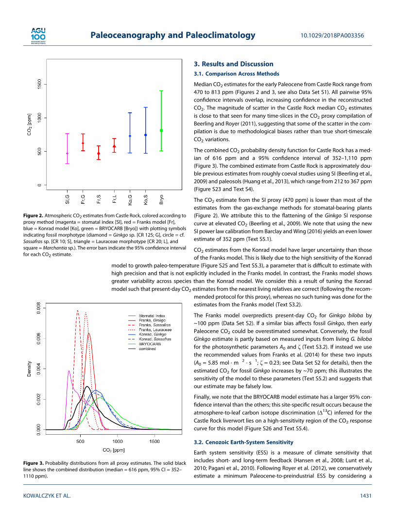
3. Results and Discussion3.1. Comparison Across Methods

Median CO2 estimates for the early Paleocene from Castle Rock range from470 to 813 ppm (Figures 2 and 3, see also Data Set S1). All pairwise 95%confidence intervals overlap, increasing confidence in the reconstructedCO2. The magnitude of scatter in the Castle Rock median CO2 estimatesis close to that seen for many time-slices in the CO2 proxy compilation ofBeerling and Royer (2011), suggesting that some of the scatter in the com-pilation is due to methodological biases rather than true short-timescaleCO2 variations.

The combined CO2 probability density function for Castle Rock has a med-ian of 616 ppm and a 95% confidence interval of 352–1,110 ppm(Figure 3). The combined estimate from Castle Rock is approximately dou-ble previous estimates from roughly coeval studies using SI (Beerling et al.,2009) and paleosols (Huang et al., 2013), which range from 212 to 367 ppm(Figure S23 and Text S4).

The CO2 estimate from the SI proxy (470 ppm) is lower than most of theestimates from the gas-exchange methods for stomatal-bearing plants(Figure 2). We attribute this to the flattening of the Ginkgo SI responsecurve at elevated CO2 (Beerling et al., 2009). We note that using the newSI power law calibration from Barclay andWing (2016) yields an even lowerestimate of 352 ppm (Text S5.1).

CO2 estimates from the Konrad model have larger uncertainty than thoseof the Franks model. This is likely due to the high sensitivity of the Konrad

model to growth paleo-temperature (Figure S25 and Text S5.3), a parameter that is difficult to estimate withhigh precision and that is not explicitly included in the Franks model. In contrast, the Franks model showsgreater variability across species than the Konrad model. We consider this a result of tuning the Konradmodel such that present-day CO2 estimates from the nearest living relatives are correct (following the recom-

mended protocol for this proxy), whereas no such tuning was done for theestimates from the Franks model (Text S3.2).

The Franks model overpredicts present-day CO2 for Ginkgo biloba by~100 ppm (Data Set S2). If a similar bias affects fossil Ginkgo, then earlyPaleocene CO2 could be overestimated somewhat. Conversely, the fossilGinkgo estimate is partly based on measured inputs from living G. bilobafor the photosynthetic parameters A0 and ζ (Text S3.2). If instead we usethe recommended values from Franks et al. (2014) for these two inputs(A0 = 5.85 mol · m�2 · s�1; ζ = 0.23; see Data Set S2 for details), then theestimated CO2 for fossil Ginkgo increases by ~70 ppm; this illustrates thesensitivity of the model to these parameters (Text S5.2) and suggests thatour estimate may be falsely low.

Finally, we note that the BRYOCARB model estimate has a larger 95% con-fidence interval than the others; this site-specific result occurs because theatmosphere-to-leaf carbon isotope discrimination (Δ13C) inferred for theCastle Rock liverwort lies on a high-sensitivity region of the CO2 responsecurve for this model (Figure S26 and Text S5.4).

3.2. Cenozoic Earth-System Sensitivity

Earth system sensitivity (ESS) is a measure of climate sensitivity thatincludes short- and long-term feedback (Hansen et al., 2008; Lunt et al.,2010; Pagani et al., 2010). Following Royer et al. (2012), we conservativelyestimate a minimum Paleocene-to-preindustrial ESS by considering a

Figure 2. Atmospheric CO2 estimates from Castle Rock, colored according toproxy method (magenta = stomatal index [SI], red = Franks model [Fr],blue = Konrad model [Ko], green = BRYOCARB [Bryo]) with plotting symbolsindicating fossil morphotype (diamond = Ginkgo sp. [CR 125; G], circle = cf.Sassafras sp. [CR 10; S], triangle = Lauraceae morphotype [CR 20; L], andsquare =Marchantia sp.). The error bars indicate the 95% confidence intervalfor each CO2 estimate.

Figure 3. Probability distributions from all proxy estimates. The solid blackline shows the combined distribution (median = 616 ppm, 95% CI = 352–1110 ppm).

10.1029/2018PA003356Paleoceanography and Paleoclimatology

KOWALCZYK ET AL. 1431

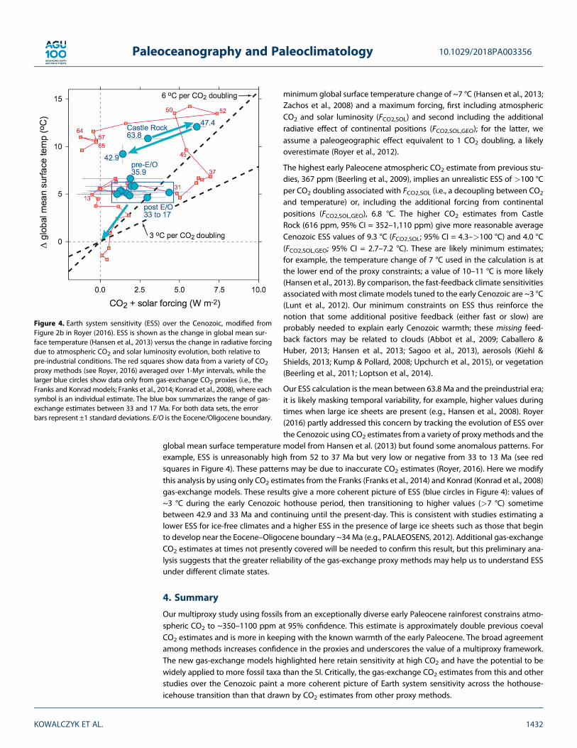
minimum global surface temperature change of ~7 °C (Hansen et al., 2013;Zachos et al., 2008) and a maximum forcing, first including atmosphericCO2 and solar luminosity (FCO2,SOL) and second including the additionalradiative effect of continental positions (FCO2,SOL,GEO); for the latter, weassume a paleogeographic effect equivalent to 1 CO2 doubling, a likelyoverestimate (Royer et al., 2012).

The highest early Paleocene atmospheric CO2 estimate from previous stu-dies, 367 ppm (Beerling et al., 2009), implies an unrealistic ESS of >100 °Cper CO2 doubling associated with FCO2,SOL (i.e., a decoupling between CO2

and temperature) or, including the additional forcing from continentalpositions (FCO2,SOL,GEO), 6.8 °C. The higher CO2 estimates from CastleRock (616 ppm, 95% CI = 352–1,110 ppm) give more reasonable averageCenozoic ESS values of 9.3 °C (FCO2,SOL; 95% CI = 4.3–>100 °C) and 4.0 °C(FCO2,SOL,GEO; 95% CI = 2.7–7.2 °C). These are likely minimum estimates;for example, the temperature change of 7 °C used in the calculation is atthe lower end of the proxy constraints; a value of 10–11 °C is more likely(Hansen et al., 2013). By comparison, the fast-feedback climate sensitivitiesassociated with most climate models tuned to the early Cenozoic are ~3 °C(Lunt et al., 2012). Our minimum constraints on ESS thus reinforce thenotion that some additional positive feedback (either fast or slow) areprobably needed to explain early Cenozoic warmth; these missing feed-back factors may be related to clouds (Abbot et al., 2009; Caballero &Huber, 2013; Hansen et al., 2013; Sagoo et al., 2013), aerosols (Kiehl &Shields, 2013; Kump & Pollard, 2008; Upchurch et al., 2015), or vegetation(Beerling et al., 2011; Loptson et al., 2014).

Our ESS calculation is the mean between 63.8 Ma and the preindustrial era;it is likely masking temporal variability, for example, higher values duringtimes when large ice sheets are present (e.g., Hansen et al., 2008). Royer(2016) partly addressed this concern by tracking the evolution of ESS overthe Cenozoic using CO2 estimates from a variety of proxy methods and the

global mean surface temperature model from Hansen et al. (2013) but found some anomalous patterns. Forexample, ESS is unreasonably high from 52 to 37 Ma but very low or negative from 33 to 13 Ma (see redsquares in Figure 4). These patterns may be due to inaccurate CO2 estimates (Royer, 2016). Here we modifythis analysis by using only CO2 estimates from the Franks (Franks et al., 2014) and Konrad (Konrad et al., 2008)gas-exchange models. These results give a more coherent picture of ESS (blue circles in Figure 4): values of~3 °C during the early Cenozoic hothouse period, then transitioning to higher values (>7 °C) sometimebetween 42.9 and 33 Ma and continuing until the present-day. This is consistent with studies estimating alower ESS for ice-free climates and a higher ESS in the presence of large ice sheets such as those that beginto develop near the Eocene–Oligocene boundary ~34 Ma (e.g., PALAEOSENS, 2012). Additional gas-exchangeCO2 estimates at times not presently covered will be needed to confirm this result, but this preliminary ana-lysis suggests that the greater reliability of the gas-exchange proxy methods may help us to understand ESSunder different climate states.

4. Summary

Our multiproxy study using fossils from an exceptionally diverse early Paleocene rainforest constrains atmo-spheric CO2 to ~350–1100 ppm at 95% confidence. This estimate is approximately double previous coevalCO2 estimates and is more in keeping with the known warmth of the early Paleocene. The broad agreementamong methods increases confidence in the proxies and underscores the value of a multiproxy framework.The new gas-exchange models highlighted here retain sensitivity at high CO2 and have the potential to bewidely applied to more fossil taxa than the SI. Critically, the gas-exchange CO2 estimates from this and otherstudies over the Cenozoic paint a more coherent picture of Earth system sensitivity across the hothouse-icehouse transition than that drawn by CO2 estimates from other proxy methods.

Figure 4. Earth system sensitivity (ESS) over the Cenozoic, modified fromFigure 2b in Royer (2016). ESS is shown as the change in global mean sur-face temperature (Hansen et al., 2013) versus the change in radiative forcingdue to atmospheric CO2 and solar luminosity evolution, both relative topre-industrial conditions. The red squares show data from a variety of CO2proxy methods (see Royer, 2016) averaged over 1-Myr intervals, while thelarger blue circles show data only from gas-exchange CO2 proxies (i.e., theFranks and Konrad models; Franks et al., 2014; Konrad et al., 2008), where eachsymbol is an individual estimate. The blue box summarizes the range of gas-exchange estimates between 33 and 17 Ma. For both data sets, the errorbars represent ±1 standard deviations. E/O is the Eocene/Oligocene boundary.

10.1029/2018PA003356Paleoceanography and Paleoclimatology

KOWALCZYK ET AL. 1432

References in Supporting Information

These references contributed to the supporting files: Arnott (1959), Bahcall et al. (2001), Barclay et al. (2003),Barclay andWing (2016), Beerling et al. (1998), Beerling et al. (2002), Beerling and Royer (2002a), Beerling et al.(2009), Beerling and Royer (2002b), Benner et al. (1987), Bowring et al. (2011), Boyce (2009), Breecker andRetallack (2014), Broadmeadow et al. (1992), Buchmann et al. (1997), Burnham and Johnson (2004),Burnham et al. (2001), Burnham et al. (1992), Carpenter et al. (2007), Chater et al. (2011), Chen et al. (2001),Clyde et al. (2016), Collister et al. (1994), Condon et al. (2015), Crifò et al. (2014), Critchfield (1970),Dechesne et al. (2011), Diefendorf et al. (2010), Dilcher (1973), Dinarès-Turell et al. (2014), Dow et al. (2014),Dunn et al. (2015), Edwards et al. (1998), Edwards (1990), Ellis et al. (2003), Ellis et al. (2004), English andJohnston (2004), Evans and Von Caemmerer (1996), Farquhar and Von Caemmerer (1982), Farquhar et al.(1980), Farquhar et al. (1989), Farquhar et al. (1982), Farquhar and Sharkey (1982), Ferguson (1985),Fletcher et al. (2005), Fletcher et al. (2004), Fletcher et al. (2008), Fletcher et al. (2006), Francey et al. (1985),Franks and Farquhar (1999), Franks et al. (2013), Franks and Beerling (2009a), Franks and Beerling (2009b),Franks et al. (2001), Franks and Farquhar (2007), Franks et al. (2014), Gardner (1975), Givnish (1988),Gradstein et al. (2012), Graham et al. (2014), Green and Snelgar (1982), Greenwood (1992), Grein et al.(2011), Haworth et al. (2011), Haworth et al. (2013), Hicks et al. (2003), Hoke et al. (2014), Holtum andWinter (2001), Huang et al. (2013), Jaffey et al. (1971), Jahren and Sternberg (2003), Johnson and Ellis(2002), Johnson et al. (2003), Kao et al. (2000), Konrad et al. (2008), Kouwenberg et al. (2007), Kürschner(1997), Larcher (1995), Leigh et al. (2011), LI-COR (2011), Lockheart et al. (1997), Long and Bernacchi (2003),Mattinson (2005), Maxbauer et al. (2014), McElwain and Chaloner (1996), McElwain et al. (2016), McLeanet al. (2011), McLean et al. (2015), Medina et al. (1986), Niinemets et al. (2009), Pagani et al. (2005),Peppe et al. (2011), Ramezani et al. (2011), Raschke and Dickerson (1973), Raven (1993, 2002), Raynolds(2002), Raynolds and Johnson (2002), Richardson et al. (2009), Roth-Nebelsick (2007), Royer (2001, 2003),Royer and Hren (2017), Royer et al. (2001), Rudall et al. (2012), Sack et al. (2006), Sack and Scoffoni(2013), Salisbury (1927), Sewall and Sloan (2006), Sharkey et al. (2007), Shobe and Lersten (1967), Smithet al. (2010), Spicer (1980), Sprain et al. (2015), Sternberg et al. (1989), Sun et al. (2003), Taylor (1999),Uhl and Mosbrugger (1999), Vanderpoorten and Goffinet (2009), Vitousek and Howarth (1991), Warrenand Adams (2006), Wilf and Johnson (2004), Woodward (1987), Wullschleger (1993), Zaiss et al. (2014),and Zeiger et al. (1987).

ReferencesAbbot, D. S., Huber, M., Bousquet, G., & Walker, C. C. (2009). High-CO2 cloud radiative forcing feedback over both land and ocean in a global

climate model. Geophysical Research Letters, 36, L05702. https://doi.org/10.1029/2008GL036703Arnott, H. J. (1959). Anastomoses in the venation of Ginkgo biloba. American Journal of Botany, 46(6), 405–411. https://doi.org/10.1002/j.1537-

2197.1959.tb07030.xAsner, G. P., Scurlock, J. M., & A Hicke, J. (2003). Global synthesis of leaf area index observations: Implications for ecological and remote

sensing studies. Global Ecology and Biogeography, 12(3), 191–205. https://doi.org/10.1046/j.1466-822X.2003.00026.xBadger, M. P., Lear, C. H., Pancost, R. D., Foster, G. L., Bailey, T. R., Leng, M. J., & Abels, H. A. (2013). CO2 drawdown following the middle

Miocene expansion of the Antarctic Ice Sheet. Paleoceanography, 28, 42–53. https://doi.org/10.1002/palo.20015Bahcall, J. N., Pinsonneault, M., & Basu, S. (2001). Solar models: Current epoch and time dependences, neutrinos, and helioseismological

properties. The Astrophysical Journal, 555, 990.Barclay, R. S., Johnson, K. R., Betterton, W. J., & Dilcher, D. L. (2003). Stratigraphy and megaflora of a K-T boundary section in the eastern

Denver Basin, Colorado. Rocky Mountain Geology, 38(1), 45–71. https://doi.org/10.2113/gsrocky.38.1.45Barclay, R. S., McElwain, J. C., & Sageman, B. B. (2010). Carbon sequestration activated by a volcanic CO2 pulse during Ocean Anoxic Event 2.

Nature Geoscience, 3(3), 205–208. https://doi.org/10.1038/ngeo757Barclay, R. S., & Wing, S. L. (2016). Improving the Ginkgo CO2 barometer: Implications for the early Cenozoic atmosphere. Earth and Planetary

Science Letters, 439, 158–171. https://doi.org/10.1016/j.epsl.2016.01.012Beerling, D., McElwain, J., & Osborne, C. (1998). Stomatal responses of the ‘living fossil’ Ginkgo biloba L. to changes in atmospheric CO2

concentrations. Journal of Experimental Botany, 49, 1603–1607.Beerling, D., & Royer, D. (2002a). Reading a CO2 signal from fossil stomata. New Phytologist, 153(3), 387–397. https://doi.org/10.1046/j.0028-

646X.2001.00335.xBeerling, D. J., Fox, A., & Anderson, C. W. (2009). Quantitative uncertainty analyses of ancient atmospheric CO2 estimates from fossil leaves.

American Journal of Science, 309(9), 775–787. https://doi.org/10.2475/09.2009.01Beerling, D. J., Fox, A., Stevenson, D. S., & Valdes, P. J. (2011). Enhanced chemistry-climate feedbacks in past greenhouse worlds. Proceedings

of the National Academy of Sciences of the United States of America, 108(24), 9770–9775. https://doi.org/10.1073/pnas.1102409108Beerling, D. J., Lomax, B. H., Royer, D. L., Upchurch, G. R. Jr., & Kump, L. R. (2002). An atmospheric pCO2 reconstruction across the Cretaceous-

Tertiary boundary from leaf megafossils. Proceedings of the National Academy of Sciences of the United States of America, 99(12), 7836–7840.https://doi.org/10.1073/pnas.122573099

Beerling, D. J., & Royer, D. L. (2002b). Fossil plants as indicators of the Phanerozoic global carbon cycle. Annual Review of Earth and PlanetarySciences, 30(1), 527–556. https://doi.org/10.1146/annurev.earth.30.091201.141413

10.1029/2018PA003356Paleoceanography and Paleoclimatology

KOWALCZYK ET AL. 1433

AcknowledgmentsWe thank R. Dunn and B. Ellis for helpfuldiscussions, A. H. Jahren for isotopicdata, S. Sultan for use of her LI-COR gas-exchange analyzer, and T. Ku forproviding laboratory space. Data andproxy model codes used in this studyare available in the SupplementaryInformation and in Kowalczyk (2018).The authors declare no conflict ofinterest.

Beerling, D. J., & Royer, D. L. (2011). Convergent Cenozoic CO2 history. Nature Geoscience, 4(7), 418–420. https://doi.org/10.1038/ngeo1186Benner, R., Fogel, M. L., Sprague, E. K., & Hodson, R. E. (1987). Depletion of

13C in lignin and its implications for stable carbon isotope studies.

Nature, 329(6141), 708–710. https://doi.org/10.1038/329708a0Bischler, H., & Boisselier-Dubayle, M. (1993). Variation in a polyploid, dioicous liverwort, Marchantia globosa. American Journal of Botany,

80(8), 953–958. https://doi.org/10.1002/j.1537-2197.1993.tb15317.xBowring, J. F., McLean, N. M., & Bowring, S. A. (2011). Engineering cyber infrastructure for U-Pb geochronology: Tripoli and U-Pb_Redux.

Geochemistry, Geophysics, Geosystems, 12, Q0AA19. https://doi.org/10.1029/2010GC003479Boyce, C. K. (2009). Seeing the forest with the leaves—Clues to canopy placement from leaf fossil size and venation characteristics.

Geobiology, 7(2), 192–199. https://doi.org/10.1111/j.1472-4669.2008.00176.xBreecker, D. O., & Retallack, G. J. (2014). Refining the pedogenic carbonate atmospheric CO2 proxy and application to Miocene CO2.

Palaeogeography, Palaeoclimatology, Palaeoecology, 406, 1–8. https://doi.org/10.1016/j.palaeo.2014.04.012Broadmeadow, M., Griffiths, H., Maxwell, C., & Borland, A. (1992). The carbon isotope ratio of plant organic material reflects temporal

and spatial variations in CO2 within tropical forest formations in Trinidad. Oecologia, 89(3), 435–441. https://doi.org/10.1007/BF00317423

Buchmann, N., Guehl, J.-M., Barigah, T., & Ehleringer, J. (1997). Interseasonal comparison of CO2 concentrations, isotopic composition,and carbon dynamics in an Amazonian rainforest (French Guiana). Oecologia, 110(1), 120–131. https://doi.org/10.1007/s004420050140

Burnham, R. J., & Johnson, K. R. (2004). South American palaeobotany and the origins of neotropical rainforests. Philosophical Transactions ofthe Royal Society B, 359(1450), 1595–1610. https://doi.org/10.1098/rstb.2004.1531

Burnham, R. J., Pitman, N. C., Johnson, K. R., & Wilf, P. (2001). Habitat-related error in estimating temperatures from leaf margins in a humidtropical forest. American Journal of Botany, 88(6), 1096–1102. https://doi.org/10.2307/2657093

Burnham, R. J., Wing, S. L., & Parker, G. G. (1992). The reflection of deciduous forest communities in leaf litter: Implications for autochthonouslitter assemblages from the fossil record. Paleobiology, 18(01), 30–49. https://doi.org/10.1017/S0094837300012203

Caballero, R., & Huber, M. (2013). State-dependent climate sensitivity in past warm climates and its implications for future climate projec-tions. Proceedings of the National Academy of Sciences of the United States of America, 110(35), 14,162–14,167. https://doi.org/10.1073/pnas.1303365110

Carpenter, R. J., Jordan, G. J., & Hill, R. S. (2007). A toothed Lauraceae leaf from the Early Eocene of Tasmania, Australia. International Journal ofPlant Sciences, 168(8), 1191–1198. https://doi.org/10.1086/520721

Chater, C., Kamisugi, Y., Movahedi, M., Fleming, A., Cuming, A. C., Gray, J. E., & Beerling, D. J. (2011). Regulatory mechanism controlling sto-matal behavior conserved across 400 million years of land plant evolution. Current Biology, 21(12), 1025–1029. https://doi.org/10.1016/j.cub.2011.04.032

Chen, L.-Q., Li, C.-S., Chaloner, W. G., Beerling, D. J., Sun, Q.-G., Collinson, M. E., & Mitchell, P. L. (2001). Assessing the potential for the stomatalcharacters of extant and fossil Ginkgo leaves to signal atmospheric CO2 change. American Journal of Botany, 88(7), 1309–1315. https://doi.org/10.2307/3558342

Clyde, W. C., Ramezani, J., Johnson, K. R., Bowring, S. A., & Jones, M. M. (2016). Direct high-precision U–Pb geochronology of the end-Cretaceous extinction and calibration of Paleocene astronomical timescales. Earth and Planetary Science Letters, 452, 272–280. https://doi.org/10.1016/j.epsl.2016.07.041

Collister, J. W., Rieley, G., Stern, B., Eglinton, G., & Fry, B. (1994). Compound-specific δ13C analyses of leaf lipids from plants with differing

carbon dioxide metabolisms. Organic Geochemistry, 21(6-7), 619–627. https://doi.org/10.1016/0146-6380(94)90008-6Condon, D. J., Schoene, B., McLean, N. M., Bowring, S. A., & Parrish, R. R. (2015). Metrology and traceability of U-Pb isotope dilution geo-

chronology (EARTHTIME Tracer Calibration Part I). Geochimica et Cosmochimica Acta, 164, 464–480. https://doi.org/10.1016/j.gca.2015.05.026

Crifò, C., Currano, E. D., Baresch, A., & Jaramillo, C. (2014). Variations in angiosperm leaf vein density have implications for interpreting lifeform in the fossil record. Geology, 42(10), 919–922. https://doi.org/10.1130/G35828.1

Critchfield, W. B. (1970). Shoot growth and heterophylly in Ginkgo biloba. Botanical Gazette, 131(2), 150–162. https://doi.org/10.1086/336526Das, S., & Sharma, G. D. (2012). Habitats of Marchantiophyta (Bryophyta) in Barail Wildlife Sanctuary, Assam: A preliminary field observation.

Assam University Journal of Science & Technology: Biological and Environmental Sciences, 9, 208–210.Dechesne, M., Raynolds, R., Barkmann, P., & Johnson, K. (2011). Denver Basin geologic maps: Bedrock Geology, Structure and isopach maps

of the Upper Cretaceous through Paleogene Strata between Greeley and Colorado Springs, Colorado. Denver, CO: Colorado GeologicalSurvey.

Diefendorf, A. F., Mueller, K. E., Wing, S. L., Koch, P. L., & Freeman, K. H. (2010). Global patterns in leaf13C discrimination and implications for

studies of past and future climate. Proceedings of the National Academy of Sciences of the United States of America, 107(13), 5738–5743.https://doi.org/10.1073/pnas.0910513107

Dilcher, D. L. (1973). A paleoclimatic interpretation of the Eocene floras of southeastern North America. In A. Graham (Ed.), Vegetation andVegetational History of Northern Latin America (pp. 39–53). Amsterdam: Elsevier.

Dinarès-Turell, J., Westerhold, T., Pujalte, V., Rohl, U., & Kroon, D. (2014). Astronomical calibration of the Danian stage (Early Paleocene)revisited: Settling chronologies of sedimentary records across the Atlantic and Pacific Oceans. Earth and Planetary Science Letters, 405,119–131. https://doi.org/10.1016/j.epsl.2014.08.027

Doria, G., Royer, D. L., Wolfe, A. P., Fox, A., Westgate, J. A., & Beerling, D. J. (2011). Declining atmospheric CO2 during the late Middle Eoceneclimate transition. American Journal of Science, 311(1), 63–75. https://doi.org/10.2475/01.2011.03

Dow, G. J., Bergmann, D. C., & Berry, J. A. (2014). An integrated model of stomatal development and leaf physiology. New Phytologist, 201(4),1218–1226. https://doi.org/10.1111/nph.12608

Dunn, R. E., Strömberg, C. A. E., Madden, R. H., Kohn, M. J., & Carlini, A. A. (2015). Linked canopy, climate, and faunal change in the Cenozoic ofPatagonia. Science, 347(6219), 258–261. https://doi.org/10.1126/science.1260947

Edwards, D., Kerp, H., & Hass, H. (1998). Stomata in early land plants: An anatomical and ecophysiological approach. Journal of ExperimentalBotany, 49(Special), 255–278. https://doi.org/10.1093/jxb/49.Special_Issue.255

Edwards, H. H. (1990). The stomatal complex of Persea borbonia. Canadian Journal of Botany, 68(12), 2543–2547. https://doi.org/10.1139/b90-320

Ellis, B., Johnson, K. R., & Dunn, R. E. (2003). Evidence for an in situ early Paleocene rainforest from Castle Rock, Colorado. Rocky MountainGeology, 38(1), 73–100. https://doi.org/10.2113/gsrocky.38.1.173

Ellis, B., Johnson, K. R., Dunn, R. E., & Reynolds, M. R. (2004). The Castle Rock Rainforest: Denver Museum of Nature & Science Technical Report2004–2.

10.1029/2018PA003356Paleoceanography and Paleoclimatology

KOWALCZYK ET AL. 1434

English, J. M., & Johnston, S. T. (2004). The Laramide orogeny: What were the driving forces? International Geology Review, 46(9), 833–838.https://doi.org/10.2747/0020-6814.46.9.833

Evans, J. R., & Von Caemmerer, S. (1996). Carbon dioxide diffusion inside leaves. Plant Physiology, 110(2), 339–346. https://doi.org/10.1104/pp.110.2.339

Farquhar, G., & Von Caemmerer, S. (1982). Modelling of photosynthetic response to environmental conditions. In O. L. Lange, P. S. Nobel, C. B.Osmond, & H. Ziegler (Eds.), Physical plant ecology II. Water relations and carbon assimilation (Vol. 2, pp. 550–587). Berlin: Springer Verlag.

Farquhar, G., von Caemmerer, S., & Berry, J. (1980). A biochemical model of photosynthetic CO2 assimilation in leaves of C3 species. Planta,149(1), 78–90. https://doi.org/10.1007/BF00386231

Farquhar, G. D., Ehleringer, J. R., & Hubick, K. T. (1989). Carbon isotope discrimination and photosynthesis. Annual Review of Plant Biology,40(1), 503–537. https://doi.org/10.1146/annurev.pp.40.060189.002443

Farquhar, G. D., O’leary, M., & Berry, J. (1982). On the relationship between carbon isotope discrimination and the intercellular carbon dioxideconcentration in leaves. Functional Plant Biology, 9, 121–137.

Farquhar, G. D., & Sharkey, T. D. (1982). Stomatal conductance and photosynthesis. Annual Review of Plant Physiology, 33(1), 317–345. https://doi.org/10.1146/annurev.pp.33.060182.001533

Ferguson, D. K. (1985). The origin of leaf-assemblages—New light on an old problem. Review of Palaeobotany and Palynology, 46(1-2),117–188. https://doi.org/10.1016/0034-6667(85)90041-7

Fletcher, B. J., Beerling, D. J., Brentnall, S. J., & Royer, D. L. (2005). Fossil bryophytes as recorders of ancient CO2 levels: Experimental evidenceand a Cretaceous case study. Global Biogeochemical Cycles, 19, GB3012. https://doi.org/10.1029/2005GB002495

Fletcher, B. J., Beerling, D. J., & Chaloner, W. (2004). Stable carbon isotopes and the metabolism of the terrestrial Devonian organismSpongiophyton. Geobiology, 2(2), 107–119. https://doi.org/10.1111/j.1472-4677.2004.00026.x

Fletcher, B. J., Brentnall, S. J., Anderson, C. W., Berner, R. A., & Beerling, D. J. (2008). Atmospheric carbon dioxide linked with Mesozoic andearly Cenozoic climate change. Nature Geoscience, 1(1), 43–48. https://doi.org/10.1038/ngeo.2007.29

Fletcher, B. J., Brentnall, S. J., Quick, W. P., & Beerling, D. J. (2006). BRYOCARB: A process-based model of thallose liverwort carbon isotopefractionation in response to CO2, O2, light and temperature. Geochimica et Cosmochimica Acta, 70(23), 5676–5691. https://doi.org/10.1016/j.gca.2006.01.031

Francey, R., Gifford, R., Sharkey, T., & Weir, B. (1985). Physiological influences on carbon isotope discrimination in huon pine (Lagarostrobosfranklinii). Oecologia, 66(2), 211–218. https://doi.org/10.1007/BF00379857

Franks, P., & Farquhar, G. (1999). A relationship between humidity response, growth form and photosynthetic operating point in C3 plants.Plant, Cell & Environment, 22(11), 1337–1349. https://doi.org/10.1046/j.1365-3040.1999.00494.x

Franks, P. J., Adams, M. A., Amthor, J. S., Barbour, M. M., Berry, J. A., Ellsworth, D. S., et al. (2013). Sensitivity of plants to changingatmospheric CO2 concentration: From the geological past to the next century. New Phytologist, 197(4), 1077–1094. https://doi.org/10.1111/nph.12104

Franks, P. J., & Beerling, D. J. (2009a). CO2-forced evolution of plant gas exchange capacity and water-use efficiency over the Phanerozoic.Geobiology, 7(2), 227–236. https://doi.org/10.1111/j.1472-4669.2009.00193.x

Franks, P. J., & Beerling, D. J. (2009b). Maximum leaf conductance driven by CO2 effects on stomatal size and density over geologic time.Proceedings of the National Academy of Sciences of the United States of America, 106(25), 10,343–10,347. https://doi.org/10.1073/pnas.0904209106

Franks, P. J., Buckley, T. N., Shope, J. C., & Mott, K. A. (2001). Guard cell volume and pressure measured concurrently by confocal microscopyand the cell pressure probe. Plant Physiology, 125(4), 1577–1584. https://doi.org/10.1104/pp.125.4.1577

Franks, P. J., & Farquhar, G. D. (2007). The mechanical diversity of stomata and its significance in gas-exchange control. Plant Physiology,143(1), 78–87. https://doi.org/10.1104/pp.106.089367

Franks, P. J., Royer, D. L., Beerling, D. J., Van de Water, P. K., Cantrill, D. J., Barbour, M. M., & Berry, J. A. (2014). New constraints on atmosphericCO2 concentration for the Phanerozoic. Geophysical Research Letters, 41, 4685–4694. https://doi.org/10.1002/2014GL060457

Fuselier, L., & McLetchie, D. N. (2004). Microhabitat and sex distribution in Marchantia inflexa, a dioicous liverwort. The Bryologist, 107(3),345–356. https://doi.org/10.1639/0007-2745(2004)107[0345:MASDIM]2.0.CO;2

Gardner, R. (1975). An overview of botanical clearing technique. Biotechnic & Histochemistry, 50, 99–105.Givnish, T. J. (1988). Adaptation to Sun and shade: A whole-plant perspective. Australian Journal of Plant Physiology, 15(2), 63–92. https://doi.

org/10.1071/PP9880063Gough, D. (1981). Solar interior structure and luminosity variations. In Physics of Solar Variations (Vol. 74, pp. 21–34). https://doi.org/10.1007/

978-94-010-9633-1_4Gradstein, F. M., Ogg, J. G., Schmitz, M., & Ogg, G. (2012). The Geologic Time Scale 2012 (Vol. 2). Amsterdam: Elsevier.Graham, H. V., Patzkowsky, M. E., Wing, S. L., Parker, G. G., Fogel, M. L., & Freeman, K. H. (2014). Isotopic characteristics of canopies in simulated

leaf assemblages. Geochimica et Cosmochimica Acta, 144, 82–95. https://doi.org/10.1016/j.gca.2014.08.032Green, T., & Snelgar, W. (1982). A comparison of photosynthesis in two thalloid liverworts. Oecologia, 54(2), 275–280. https://doi.org/10.1007/

BF00378404Greenwood, D. R. (1992). Taphonomic constraints on foliar physiognomic interpretations of Late Cretaceous and Tertiary palaeoclimates.

Review of Palaeobotany and Palynology, 71(1-4), 149–190. https://doi.org/10.1016/0034-6667(92)90161-9Grein, M., Konrad, W., Wilde, V., Utescher, T., & Roth-Nebelsick, A. (2011). Reconstruction of atmospheric CO2 during the early middle Eocene

by application of a gas exchange model to fossil plants from the Messel Formation, Germany. Palaeogeography, Palaeoclimatology,Palaeoecology, 309(3-4), 383–391. https://doi.org/10.1016/j.palaeo.2011.07.008

Hansen, J., Sato, M., Kharecha, P., Beerling, D., Berner, R., Masson-Delmotte, V., et al. (2008). Target atmospheric CO2: Where should humanityaim? Open Atmospheric Science Journal, 2(1), 217–231. https://doi.org/10.2174/1874282300802010217

Hansen, J., Sato, M., Russell, G., & Kharecha, P. (2013). Climate sensitivity, sea level and atmospheric carbon dioxide. Philosophical Transactionsof the Royal Society A, 371(2001), 20120294. https://doi.org/10.1098/rsta.2012.0294

Haworth, M., Elliott-Kingston, C., & McElwain, J. C. (2011). Stomatal control as a driver of plant evolution. Journal of Experimental Botany, 62(8),2419–2423. https://doi.org/10.1093/jxb/err086

Haworth, M., Elliott-Kingston, C., & McElwain, J. C. (2013). Co-ordination of physiological andmorphological responses of stomata to elevated[CO2] in vascular plants. Oecologia, 171(1), 71–82. https://doi.org/10.1007/s00442-012-2406-9

Hicks, J. F., Johnson, K. R., Obradovich, J. D., Miggins, D. P., & Tauxe, L. (2003). Magnetostratigraphy of upper Cretaceous (Maastrichtian) tolower Eocene strata of the Denver Basin, Colorado. Rocky Mountain Geology, 38(1), 1–27. https://doi.org/10.2113/gsrocky.38.1.1

Hoke, G. D., Schmitz, M. D., & Bowring, S. A. (2014). An ultrasonic method for isolating nonclay components from clay-rich material.Geochemistry, Geophysics, Geosystems, 15, 492–498. https://doi.org/10.1002/2013GC005125

10.1029/2018PA003356Paleoceanography and Paleoclimatology

KOWALCZYK ET AL. 1435

Holtum, J., & Winter, K. (2001). Are plants growing close to the floors of tropical forests exposed to markedly elevated concentrations ofcarbon dioxide? Australian Journal of Botany, 49(5), 629–636. https://doi.org/10.1071/BT00054

Huang, C., Retallack, G. J., Wang, C., & Huang, Q. (2013). Paleoatmospheric pCO2 fluctuations across the Cretaceous–Tertiary boundaryrecorded from paleosol carbonates in NE China. Palaeogeography, Palaeoclimatology, Palaeoecology, 385, 95–105. https://doi.org/10.1016/j.palaeo.2013.01.005

Intergovernmental Panel on Climate Change (2014). Climate change 2014: Synthesis report. Contribution of Working Groups I, II and III to theFifth Assessment Report of the Intergovernmental Panel on Climate Change. In R. K. Pachauri & L. A. Meyer (Eds.) (p. 151). Geneva,Switzerland: IPCC.

Jaffey, A. H., Flynn, K. F., Glendenin, L. E., Bentley, W. C., & Essling, A. M. (1971). Precision measurement of half-lives and specific activities of235

U and238

U. Physical Review C, 4(5), 1889–1906. https://doi.org/10.1103/PhysRevC.4.1889Jahren, A. H., & Sternberg, L. S. L. (2003). Humidity estimate for the middle Eocene Arctic rain forest. Geology, 31(5), 463–466. https://doi.org/

10.1130/0091-7613(2003)031<0463:HEFTME>2.0.CO;2Johnson, K. R., & Ellis, B. (2002). A tropical rainforest in Colorado 1.4 million years after the Cretaceous-Tertiary boundary. Science, 296(5577),

2379–2383. https://doi.org/10.1126/science.1072102Johnson, K. R., Reynolds, M. L., Werth, K. W., & Thomasson, J. R. (2003). Overview of the Late Cretaceous, early Paleocene, and early Eocene

megafloras of the Denver Basin, Colorado. Rocky Mountain Geology, 38(1), 101–120. https://doi.org/10.2113/gsrocky.38.1.101Kao, W.-Y., Chiu, Y.-S., & Chen, W.-H. (2000). Vertical profiles of CO2 concentration and δ

13C values in a subalpine forest of Taiwan. Botanical

Bulletin of Academia Sinica, 41, 213–218.Kiehl, J. T., & Shields, C. A. (2013). Sensitivity of the Palaeocene–Eocene Thermal Maximum climate to cloud properties. Philosophical

Transactions of the Royal Society A, 371(2001), 20130093. https://doi.org/10.1098/rsta.2013.0093Konrad, W., Roth-Nebelsick, A., & Grein, M. (2008). Modelling of stomatal density response to atmospheric CO2. Journal of Theoretical Biology,

253(4), 638–658. https://doi.org/10.1016/j.jtbi.2008.03.032Kouwenberg, L. L. R., Hines, R. R., & McElwain, J. C. (2007). A new transfer technique to extract and process thin and fragmented fossil cuticle

using polyester overlays. Review of Palaeobotany and Palynology, 145(3-4), 243–248. https://doi.org/10.1016/j.revpalbo.2006.11.002Kowalczyk, J. (2018). Castle Rock (Version 1). figshare. https://doi.org/10.6084/m9.figshare.c.4002252.v1Kump, L. R., & Pollard, D. (2008). Amplification of Cretaceous warmth by biological cloud feedbacks. Science, 320(5873), 195–195. https://doi.

org/10.1126/science.1153883Kürschner, W. M. (1997). The anatomical diversity of recent and fossil leaves of the durmast oak (Quercus petraea Lieblein/Q. pseudocastanea

Goeppert)-implications for their use as biosensors of palaeoatmospheric CO2 levels. Review of Palaeobotany and Palynology, 96(1-2), 1–30.https://doi.org/10.1016/S0034-6667(96)00051-6

Kürschner, W. M., Kvaček, Z., & Dilcher, D. L. (2008). The impact of Miocene atmospheric carbon dioxide fluctuations on climate and theevolution of terrestrial ecosystems. Proceedings of the National Academy of Sciences of the United States of America, 105(2), 449–453.https://doi.org/10.1073/pnas.0708588105

Lacis, A. A., Schmidt, G. A., Rind, D., & Ruedy, R. A. (2010). Atmospheric CO2: Principal control knob governing Earth’s temperature. Science,330(6002), 356–359. https://doi.org/10.1126/science.1190653

Larcher, W. (1995). Physiological Plant Ecology: Ecophysiology and Stress Physiology of Functional Groups, (3rd ed.). Berlin, New York: Springer-Verlag. https://doi.org/10.1007/978-3-642-87851-0

Leigh, A., Zwieniecki, M. A., Rockwell, F. E., Boyce, C. K., Nicotra, A. B., & Holbrook, N. M. (2011). Structural and hydraulic correlates of het-erophylly in Ginkgo biloba. New Phytologist, 189(2), 459–470. https://doi.org/10.1111/j.1469-8137.2010.03476.x

LI-COR (2011). Using the LI-6400/LI-6400XT portable photosynthesis system, Version 6.Lockheart, M. J., Van Bergen, P. F., & Evershed, R. P. (1997). Variations in the stable carbon isotope compositions of individual lipids from the

leaves of modern angiosperms: Implications for the study of higher land plant-derived sedimentary organic matter. Organic Geochemistry,26(1-2), 137–153. https://doi.org/10.1016/S0146-6380(96)00135-0

Long, S. P., & Bernacchi, C. J. (2003). Gas exchange measurements, what can they tell us about the underlying limitations to photo-synthesis? Procedures and sources of error. Journal of Experimental Botany, 54(392), 2393–2401. https://doi.org/10.1093/jxb/erg262

Loptson, C., Lunt, D., & Francis, J. (2014). Investigating vegetation–climate feedbacks during the early Eocene. Climate of the Past, 10(2),419–436. https://doi.org/10.5194/cp-10-419-2014

Lunt, D. J., Dunkley Jones, T., Heinemann, M., Huber, M., LeGrande, A., Winguth, A., et al. (2012). A model–data comparison for a multi-modelensemble of early Eocene atmosphere–ocean simulations: EoMIP. Climate of the Past, 8(5), 1717–1736. https://doi.org/10.5194/cp-8-1717-2012

Lunt, D. J., Haywood, A. M., Schmidt, G. A., Salzmann, U., Valdes, P. J., & Dowsett, H. J. (2010). Earth system sensitivity inferred from Pliocenemodelling and data. Nature Geoscience, 3(1), 60–64. https://doi.org/10.1038/ngeo706

Luthi, D., Le Floch, M., Bereiter, B., Blunier, T., Barnola, J. M., Siegenthaler, U., et al. (2008). High-resolution carbon dioxide concentration record650,000-800,000 years before present. Nature, 453(7193), 379–382. https://doi.org/10.1038/nature06949

Mattinson, J. M. (2005). Zircon U/Pb chemical abrasion (CA-TIMS) method; combined annealing and multi-step partial dissolutionanalysis for improved precision and accuracy of zircon ages. Chemical Geology, 220(1-2), 47–66. https://doi.org/10.1016/j.chemgeo.2005.03.011

Maxbauer, D. P., Royer, D. L., & LePage, B. A. (2014). High Arctic forests during the middle Eocene supported by moderate levels of atmo-spheric CO2. Geology, 42(12), 1027–1030. https://doi.org/10.1130/G36014.1

McElwain, J. C., & Chaloner, W. G. (1996). The fossil cuticle as a skeletal record of environmental change. PALAIOS, 11(4), 376–388. https://doi.org/10.2307/3515247

McElwain, J. C., Yiotis, C., & Lawson, T. (2016). Using modern plant trait relationships between observed and theoretical maximum stomatalconductance and vein density to examine patterns of plant macroevolution. New Phytologist, 209(1), 94–103. https://doi.org/10.1111/nph.13579

McLean, N. M., Bowring, J. F., & Bowring, S. A. (2011). An algorithm for U-Pb isotope dilution data reduction and uncertainty propagation.Geochemistry, Geophysics, Geosystems, 12, Q0AA18. https://doi.org/10.1029/2010GC003478

McLean, N. M., Condon, D. J., Schoene, B., & Bowring, S. A. (2015). Evaluating uncertainties in the calibration of isotopic reference materialsandmulti-element isotopic tracers (EARTHTIME Tracer Calibration Part II). Geochimica et Cosmochimica Acta, 164, 481–501. https://doi.org/10.1016/j.gca.2015.02.040

Medina, E., Montes, G., Cuevas, E., & Rokzandic, Z. (1986). Profiles of CO2 concentration and δ13C values in tropical rain forests of the upper Rio

Negro Basin, Venezuela. Journal of Tropical Ecology, 2(03), 207–217. https://doi.org/10.1017/S0266467400000821

10.1029/2018PA003356Paleoceanography and Paleoclimatology

KOWALCZYK ET AL. 1436

Montañez, I. P., Norris, R. D., Algeo, T., Chandler, M. A., Johnson, K. R., Kennedy, M. J., et al. (2011). Understanding Earth’s deep past: Lessons forour climate future. Washington, DC: National Academies Press.

Niinemets, Ü., Díaz-Espejo, A., Flexas, J., Galmés, J., & Warren, C. R. (2009). Role of mesophyll diffusion conductance in constrainingpotential photosynthetic productivity in the field. Journal of Experimental Botany, 60(8), 2249–2270. https://doi.org/10.1093/jxb/erp036

Pagani, M., Liu, Z., LaRiviere, J., & Ravelo, A. C. (2010). High Earth-system climate sensitivity determined from Pliocene carbon dioxide con-centrations. Nature Geoscience, 3(1), 27–30. https://doi.org/10.1038/ngeo724

Pagani, M., Zachos, J. C., Freeman, K. H., Tipple, B., & Bohaty, S. (2005). Marked decline in atmospheric carbon dioxide concentrations duringthe Paleogene. Science, 309(5734), 600–603. https://doi.org/10.1126/science.1110063

PALAEOSENS (2012). Making sense of palaeoclimate sensitivity. Nature, 491(7426), 683–691. https://doi.org/10.1038/nature11574Peppe, D. J., Royer, D. L., Cariglino, B., Oliver, S. Y., Newman, S., Leight, E., et al. (2011). Sensitivity of leaf size and shape to climate: Global

patterns and paleoclimatic applications. New Phytologist, 190(3), 724–739. https://doi.org/10.1111/j.1469-8137.2010.03615.xRamezani, J., Hoke, G. D., Fastovsky, D. E., Bowring, S. A., Therrien, F., Dworkin, S. I., et al. (2011). High-precision U-Pb zircon geochronology of

the Late Triassic Chinle Formation, Petrified Forest National Park (Arizona, USA): Temporal constraints on the early evolution of dinosaurs.Geological Society of America Bulletin, 123(11-12), 2142–2159. https://doi.org/10.1130/B30433.1

Raschke, K., & Dickerson, M. (1973). Changes in shape and volume of guard cells during stomatal movement. In Plant research. Report of theMSU/AEC Plant Research Laboratory (pp. 153–155). East Lansing: Michigan State University.

Raven, J. A. (1993). The evolution of vascular plants in relation to quantitative functioning of dead water-conducting cells and stomata.Biological Reviews, 68(3), 337–363. https://doi.org/10.1111/j.1469-185X.1993.tb00735.x

Raven, J. A. (2002). Selection pressures on stomatal evolution. New Phytologist, 153(3), 371–386. https://doi.org/10.1046/j.0028-646X.2001.00334.x

Raynolds, R. G. (2002). Upper Cretaceous and Tertiary stratigraphy of the Denver basin, Colorado. Rocky Mountain Geology, 37(2), 111–134.https://doi.org/10.2113/3

Raynolds, R. G., & Johnson, K. R. (2002). Drilling of the Kiowa Core, Elbert County, Colorado. Rocky Mountain Geology, 37(2), 105–109. https://doi.org/10.2113/2

Richards, P. W. (1996). The Tropical Rain Forest: An Ecological Study (2nd ed.). Cambridge, UK: Cambridge University Press.Richardson, A. D., Hollinger, D. Y., Dail, D. B., Lee, J. T., Munger, J. W., & O’Keefe, J. (2009). Influence of spring phenology on seasonal and

annual carbon balance in two contrasting New England forests. Tree Physiology, 29(3), 321–331. https://doi.org/10.1093/treephys/tpn040

Roth-Nebelsick, A. (2007). Computer-based studies of diffusion through stomata of different architecture. Annals of Botany, 100(1), 23–32.https://doi.org/10.1093/aob/mcm075

Royer, D. L. (2001). Stomatal density and stomatal index as indicators of paleoatmospheric CO2 concentration. Review of Palaeobotany andPalynology, 114(1-2), 1–28. https://doi.org/10.1016/S0034-6667(00)00074-9

Royer, D. L. (2003). Estimating latest Cretaceous and Tertiary atmospheric CO2 from stomatal indices. Geological Society of America SpecialPapers, 369, 79–94.

Royer, D. L. (2016). Climate sensitivity in the geologic past. Annual Review of Earth and Planetary Sciences, 44(1), 277–293. https://doi.org/10.1146/annurev-earth-100815-024150

Royer, D. L., & Hren, M. T. (2017). Carbon isotopic fractionation between whole leaves and cuticle. PALAIOS, 32(4), 199–205. https://doi.org/10.2110/palo.2016.073

Royer, D. L., Pagani, M., & Beerling, D. J. (2012). Geobiological constraints on Earth system sensitivity to CO2 during the Cretaceous andCenozoic. Geobiology, 10(4), 298–310. https://doi.org/10.1111/j.1472-4669.2012.00320.x

Royer, D. L., Wing, S. L., Beerling, D. J., Jolley, D. W., Koch, P. L., Hickey, L. J., & Berner, R. A. (2001). Paleobotanical evidence for nearpresent-day levels of atmospheric CO2 during part of the Tertiary. Science, 292(5525), 2310–2313. https://doi.org/10.1126/science.292.5525.2310

Rudall, P. J., Rowland, A., & Bateman, R. M. (2012). Ultrastructure of stomatal development in Ginkgo biloba. International Journal of PlantSciences, 173(8), 849–860. https://doi.org/10.1086/667230

Sack, L., Melcher, P. J., Liu, W. H., Middleton, E., & Pardee, T. (2006). How strong is intracanopy leaf plasticity in temperate deciduous trees?American Journal of Botany, 93(6), 829–839. https://doi.org/10.3732/ajb.93.6.829

Sack, L., & Scoffoni, C. (2013). Leaf venation: Structure, function, development, evolution, ecology and applications in the past, present andfuture. New Phytologist, 198(4), 983–1000. https://doi.org/10.1111/nph.12253

Sagoo, N., Valdes, P., Flecker, R., & Gregoire, L. J. (2013). The Early Eocene equable climate problem: Can perturbations of climate modelparameters identify possible solutions? Philosophical Transactions of the Royal Society A, 371, 20130123. https://doi.org/10.1098/rsta.2013.0123

Salisbury, E. J. (1927). On the causes and ecological significance of stomatal frequency, with special reference to the woodland flora.Philosophical Transactions of the Royal Society B, 216, 1–65.

Schubert, B. A., & Jahren, A. H. (2018). Incorporating the effects of photorespiration into terrestrial paleoclimate reconstruction. Earth-ScienceReviews, 177, 637–642. https://doi.org/10.1016/j.earscirev.2017.12.008

Seki, O., Foster, G. L., Schmidt, D. N., Mackensen, A., Kawamura, K., & Pancost, R. D. (2010). Alkenone and boron-based Pliocene pCO2 records.Earth and Planetary Science Letters, 292(1-2), 201–211. https://doi.org/10.1016/j.epsl.2010.01.037

Sewall, J. O., & Sloan, L. C. (2006). Come a little bit closer: A high-resolution climate study of the early Paleogene Laramide foreland. Geology,34(2), 81–84. https://doi.org/10.1130/G22177.1

Sharkey, T. D., Bernacchi, C. J., Farquhar, G. D., & Singsaas, E. L. (2007). Fitting photosynthetic carbon dioxide response curves for C3 leaves.Plant, Cell & Environment, 30(9), 1035–1040. https://doi.org/10.1111/j.1365-3040.2007.01710.x

Shobe, W. R., & Lersten, N. R. (1967). A technique for clearing and staining gymnosperm leaves. Botanical Gazette, 128(2), 150–152. https://doi.org/10.1086/336391

Siregar, E. S., Ariyanti, N. S., & Tjitrosoedirdjo, S. S. (2013). The liverwort genusMarchantia (Marchantiaceae) of mount Sibayak, North Sumatra,Indonesia. Biotropia, 20, 73–80.

Smith, R. Y., Greenwood, D. R., & Basinger, J. F. (2010). Estimating paleoatmospheric pCO2 during the Early Eocene Climatic Optimum fromstomatal frequency of Ginkgo, Okanagan Highlands, British Columbia, Canada. Palaeogeography, Palaeoclimatology, Palaeoecology,293(1-2), 120–131. https://doi.org/10.1016/j.palaeo.2010.05.006

Spicer, R. A. (1980). The importance of depositional sorting to the biostratigraphy of plant megafossils. In D. Dilcher & T. Taylor (Eds.),Biostratigraphy of fossil plants: Successional and paleoecological analyses (pp. 171–183). Stroudsburg, PA: Dowden, Hutchinson, and Ross.

10.1029/2018PA003356Paleoceanography and Paleoclimatology

KOWALCZYK ET AL. 1437

Sprain, C. J., Renne, P. R., Wilson, G. P., & Clemens, W. A. (2015). High-resolution chronostratigraphy of the terrestrial Cretaceous-Paleogenetransition and recovery interval in the Hell Creek region, Montana. Geological Society of America Bulletin, 127(3-4), 393–409. https://doi.org/10.1130/B31076.1

Sternberg, L. S. L., Mulkey, S. S., & Wright, S. J. (1989). Ecological interpretation of leaf carbon isotope ratios: Influence of respired carbondioxide. Ecology, 70, 1317–1324.

Sun, B., Dilcher, D. L., Beerling, D. J., Zhang, C., Yan, D., & Kowalski, E. (2003). Variation in Ginkgo biloba L. leaf characters across a climaticgradient in China. Proceedings of the National Academy of Sciences of the United States of America, 100(12), 7141–7146. https://doi.org/10.1073/pnas.1232419100

Taylor, T. (1999). The ultrastructure of fossil cuticle. In T. Jones & N. Rowe (Eds.), Fossil plants and spores: Modern techniques (pp. 113–115).Bath, UK: Geological Society of London.

Tipple, B. J., Meyers, S. R., & Pagani, M. (2010). Carbon isotope ratio of Cenozoic CO2: A comparative evaluation of available geochemicalproxies. Paleoceanography, 25, PA3202. https://doi.org/10.1029/2009PA001851

Uhl, D., & Mosbrugger, V. (1999). Leaf venation density as a climate and environmental proxy: A critical review and new data.Palaeogeography Palaeoclimatology Palaeoecology, 149(1-4), 15–26. https://doi.org/10.1016/S0031-0182(98)00189-8

Upchurch, G. R., Kiehl, J., Shields, C., Scherer, J., & Scotese, C. (2015). Latitudinal temperature gradients and high-latitude temperatures duringthe latest Cretaceous: Congruence of geologic data and climate models. Geology, 43(8), 683–686. https://doi.org/10.1130/G36802.1

van Hinsbergen, D. J., de Groot, L. V., van Schaik, S. J., Spakman, W., Bijl, P. K., Sluijs, A., et al. (2015). A paleolatitude calculator for paleoclimatestudies. PLoS One, 10(6), e0126946. https://doi.org/10.1371/journal.pone.0126946

Vanderpoorten, A., & Goffinet, B. (2009). Introduction to Bryophytes, Vol 1. Cambridge, UK: Cambridge University Press. https://doi.org/10.1017/CBO9780511626838

Vitousek, P. M., & Howarth, R. W. (1991). Nitrogen limitation on land and in the sea: How can it occur? Biogeochemistry, 13, 87–115.Warren, C. R., & Adams, M. A. (2006). Internal conductance does not scale with photosynthetic capacity: Implications for carbon isotope

discrimination and the economics of water and nitrogen use in photosynthesis. Plant, Cell & Environment, 29(2), 192–201. https://doi.org/10.1111/j.1365-3040.2005.01412.x

Wilf, P. (1997). When are leaves good thermometers? A new case for leaf margin analysis. Paleobiology, 23(03), 373–390. https://doi.org/10.1017/S0094837300019746

Wilf, P., & Johnson, K. R. (2004). Land plant extinction at the end of the Cretaceous: A quantitative analysis of the North Dakota megafloralrecord. Paleobiology, 30(3), 347–368. https://doi.org/10.1666/0094-8373(2004)030<0347:LPEATE>2.0.CO;2

Woodward, F. I. (1987). Stomatal numbers are sensitive to increases in CO2 from pre-industrial levels. Nature, 327(6123), 617–618. https://doi.org/10.1038/327617a0

Wullschleger, S. D. (1993). Biochemical limitations to carbon assimilation in C3 plants—A retrospective analysis of the A/Ci curves from 109species. Journal of Experimental Botany, 44(5), 907–920. https://doi.org/10.1093/jxb/44.5.907

Zachos, J. C., Dickens, G. R., & Zeebe, R. E. (2008). An early Cenozoic perspective on greenhouse warming and carbon-cycle dynamics. Nature,451(7176), 279–283. https://doi.org/10.1038/nature06588

Zaiss, J., Ravizza, G., Goderis, S., Sauvage, J., Claeys, P., & Johnson, K. (2014). A complete Os excursion across a terrestrial Cretaceous-Paleogene boundary at the West Bijou Site, Colorado, with evidence for recent open system behavior. Chemical Geology, 385, 7–16.https://doi.org/10.1016/j.chemgeo.2014.07.010

Zeiger, E., Farquhar, G. D., & Cowan, I. R. (1987). Stomatal Function. CA: Stanford University Press.

10.1029/2018PA003356Paleoceanography and Paleoclimatology

KOWALCZYK ET AL. 1438