Part 2: Analysis of Relationship Between Two Variablesyu/class/ess210b/lecture.3.regression.all.pdf · Part 2: Analysis of Relationship Between Two Variables ... After perform the

ESS210BESS210BProf. JinProf. Jin--Yi YuYi Yu

Part 2: Analysis of Relationship Part 2: Analysis of Relationship Between Two VariablesBetween Two Variables

Linear Regression

Linear correlation

Significance Tests

Multiple regression


Linear RegressionLinear Regression

Y = a X + b

• To find the relationship between Y and X which yields values of Y with the least error.

DependentVariable

IndependentVariable


Predictor and Predictor and PredictandPredictand

In meteorology, we want to use a variable x to predict another variable y. In this case, the independent variable xis called the “predictor”. The dependent variable y is called the “predictand”

Y = a + b X

the independent variablethe predictor

the dependent variablethe predictand


Linear RegressionLinear Regression

We have N paired data point (xi, yi)that we want to approximate their relationship with a linear regression:

The errors produced by this linear approximation can be estimated as:

The least square linear fit chooses coefficients a and b to produce a minimum value of the error Q.

a0 = intercepta1 = slope (b)


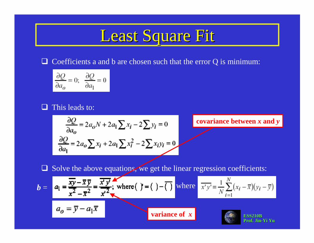
Least Square FitLeast Square FitCoefficients a and b are chosen such that the error Q is minimum:

This leads to:

Solve the above equations, we get the linear regression coefficients:

where

covariance between x and y

variance of x

b =


ExampleExample


RR22--valuevalue

R2-value measures the percentage of variation in the values of the dependent variable that can be explained by the variation in the independent variable.R2-value varies from 0 to 1.A value of 0.7654 means that 76.54% of the variance in y can be explained by the changes in X. The remaining 23.46% of the variation in y is presumed to be due to random variability.


Significance of the Regression CoefficientsSignificance of the Regression Coefficients

There are many ways to test the significance of the regression coefficient.

Some use t-test to test the hypothesis that b=0.

The most useful way for the test the significance of the regression is use the “analysis of variance” which separates the total variance of the dependent variable into two independent parts: variance accounted for by the linear regression and the error variance.


How Good Is the Fit?How Good Is the Fit?The quality of the linear regression can be analyzed using the “Analysis of Variance”.

The analysis separates the total variance of y (Sy

2) into the part that can be accounted for by the linear regression (b2Sx

2) and the part that can not be accounted for by the regression (Sε

2):

Sy2 = b2Sx

2 + Sε2

0


Variance AnalysisVariance Analysis

To calculate the total variance, we need to know the “mean” DOF=N-1If we know the mean and the regression slope (B), then the regression line is set The DOF of the regressed variance is only 1 (the slope).The error variance is determined from the difference between the total variance (with DOF = N-1) and the regressed variance (DOF=1) The DOF of the error variance = (N-1)-1=N-2.


Analysis of Variance (ANOVA)Analysis of Variance (ANOVA)

We then use F-statistics to test the ratio of the variance explained by the regression and the variance not explained by the regression:

F = (b2Sx2/1) / (Sε

2/(N-2))

Select a X% confidence level

H0: β = 0 (i.e., variation in y is not explained by the linear regression butrather by chance or fluctuations)

H1: β ≠ 0

Reject the null hypothesis at the α significance level if F>Fα(1, N-2)

regression slope in population


ExampleExample


ScatteringScatteringOne way to estimate the “badness of fit” is to calculate the scatter:

scatter Sscatter =

The relation between the scatter to the line of regression in the analysis of two variables is like the relation between the standard deviation to the mean in the analysis of one variable.

If lines are drawn parallel to the line of regression at distances equal to ± (Sscatter)0.5

above and below the line, measured in the y direction, about 68% of the observation should fall between the two lines.

0123456789

101112

0 2 4 6 8 10 12

X

Y

Sε


Correlation and RegressionCorrelation and RegressionLinear Regression: Y = a + bXA dimensional measurement of the linear relationship between X and Y.How does Y change with one unit of X?

Linear CorrelationA non-dimensional measurement of the linear relationship between X and Y.How does Y change (in standard deviation) with one standard deviation of X?


Linear CorrelationLinear Correlation

The linear regression coefficient (b) depends on the unit of measurement.

If we want to have a non-dimensional measurement of the association between two variables, we use the linear correlation coefficient (r):


Correlation and RegressionCorrelation and RegressionRecall in the linear regression, we show that:

We also know:

It turns out that

the fraction of the variance of yexplained by linear regression

The square of the correlation coefficient is equal to the fraction of variance explained by a linear least-squares fit between two variables.


An ExampleAn Example

Suppose that the correlation coefficient between sunspots and five-year mean global temperature is 0.5 ( r = 0.5 ).

The fraction of the variance of 5-year mean global temperature that is “explained” by sunspots is r2 = 0.25.

The fraction of unexplained variance is 0.75.


Significance Test of Correlation CoefficientSignificance Test of Correlation Coefficient

When the true correlation coefficient is zero (H0: ρ=0 and H1: ρ≠0)Use Student-t to test the significance of r

and ν = N-2 degree of freedom

When the true correlation coefficient is notis not expected to be zeroWe can not use a symmetric normal distribution for the test.

We must use Fisher’s Z transformation to convert the distribution of rto a normal distribution:

mean of Z std of Z


An ExampleAn ExampleSuppose N = 21 and r = 0.8. Find the 95% confidence limits on r.

Answer:(1) Use Fisher’s Z transformation:

(2) Find the 95% significance limits

(3) Convert Z back to r

(4) The 95% significance limits are: 0.56 < ρ < 0.92

a handy way toconvert Z back to r


Another ExampleAnother ExampleIn a study of the correlation between the amount of rainfall and the quality of air pollution removed, 9 observations were made. The sample correlation coefficient is –0.9786. Test the null hypothesis that there is no linear correlation between the variables. Use 0.05 level of significance.

Answer:1. Ho: ρ = 0; H1: ρ≠ 02. α = 0.053. Use Fisher’s Z

4. Z < Z 0.025 (= -1.96) Reject the null hypothesis


Test of the Difference Between Two Test of the Difference Between Two NonNon--Zero CoefficientsZero Coefficients

We first convert r to Fisher’s Z statistics:

We then assume a normal distribution for Z1-Z2 and use the z-statistic (not Fisher’s Z):


Multiple RegressionMultiple RegressionIf we want to regress y with more than one variables (x1, x2, x3,…..xn):

After perform the least-square fit and remove means from all variables:

Solve the following matrix to obtain the regression coefficients: a1, a2, a3, a4,….., an:


Fourier TransformFourier TransformFourier transform is an example of multiple regression. In this case, the independent (predictor) variables are:

These independent variables are orthogonal to each other. That means:

Therefore, all the off-diagonal terms are zero in the following matrix:

We can easily get:

This demonstrates Fourier analysis is optimal in least square sense.


How Many Predictors Are Needed?How Many Predictors Are Needed?Very often, one predictor is a function of the other predictors.

It becomes an important question: How many predictors do we need in order to make a good regression (or prediction)?

Does increasing the number of the predictor improve the regression (or prediction)?

If too many predictors are used, some large coefficients may be assigned to variables that are not really highly correlated to the predictant (y). These coefficients are generated to help the regression relation to fit y.

To answer this question, we have to figure out how fast (or slow) the “fraction of explained variance” increase with additional number of predictors.


Explained Variance for Multiple RegressionExplained Variance for Multiple Regression

As an example, we discuss the case of two predictors for the multiple regression.

We can repeat the derivation we perform for the simple linear regression to find that the fraction of variance explained by the 2-predictors regression (R) is:

here r is the correlation coefficient

We can show that if r2y is smaller than or equal to a “minimum useful correlation” value, it is not useful to include the second predictor in the regression.

The minimum useful correlation = r1y * r12This is the minimum correlation of x2 with y that is required to improve the R2 given that x2 is correlated with x1.

We want r2y > r1y * r12


An ExampleAn Example

For a 2-predictor case: r1y = r2y = r12 = 0.50If only include one predictor (x1) (r2y = r12 =0) R2=0.25By adding x2 in the regression (r2y = r12 =0.50) R2=0.33In this case, the 2nd predictor improve the regression.

For a 2-predictor case: r1y = r12 = 0.50 but r2y = 0.25If with only x1 R2=025Adding x2 R2=025 (still the same!!)In this case, the 2nd predictor is not useful. It is becauser2y ≤ r1y * r12 = 0.50*0.50 = 0.25


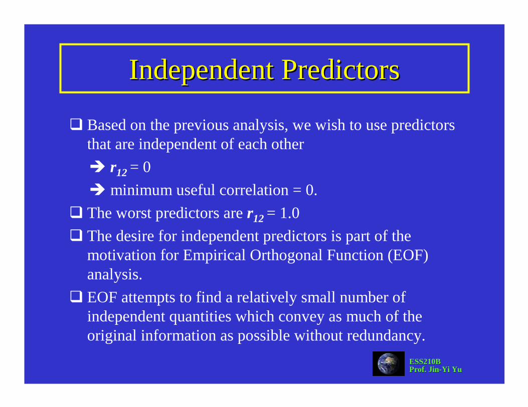
Independent PredictorsIndependent Predictors

Based on the previous analysis, we wish to use predictors that are independent of each other

r12 = 0 minimum useful correlation = 0.

The worst predictors are r12 = 1.0The desire for independent predictors is part of the motivation for Empirical Orthogonal Function (EOF) analysis.EOF attempts to find a relatively small number of independent quantities which convey as much of the original information as possible without redundancy.

Documents

Part 2: Analysis of Relationship Between Two Variablesyu/class/ess210b/lecture.3.regression.all.pdf · Part 2: Analysis of Relationship Between Two Variables ... After perform the