Embed Size (px)
Citation preview

Astronomische Waarneemtechnieken (Astronomical Observing Techniques)
6th Lecture: 8 October 2012
Based on “Astronomical Optics” by Daniel J. Schroeder, “Principles of
Reference” by William L. Wolfe, Lena book, and Wikipedia
1. Geometrical Optics Definitions Aberrations
2. Diffraction Optics Fraunhofer Diff. PSF, MTF SR & EE high contrast im.
Part I Geometrical Optics
Part II Diffraction Optics

Aperture stop: determines the diameter of the light cone from an axial point on the object. Field stop: determines the field of view of the system. Entrance pupil: image of the aperture stop in the object space Exit pupil: image of the aperture stop in the image space Marginal ray: ray from an object point on the optical axis that passes at the edge of the entrance pupil Chief ray: ray from an object point at the edge of the field, passing through the center of the aperture stop.
Aperture and Field Stops
camera telescope

The speed of an optical system is described by the numerical aperture NA and the F number, where:
NA)(21 and sinNA
DfFn
The Speed of the System f
D
Generally, fast optics (large NA) has a high light power, is compact, but has tight tolerances and is difficult to manufacture. Slow optics (small NA) is just the opposite.
Étendue and Ax The geometrical étendue (frz. ̀ extent is the product of area A of the source times the solid angle (of the system's entrance pupil as seen from the source). The étendue is the maximum beam size the instrument can accept. Hence, the étendue is also called acceptance, throughput, or Aproduct. The étendue never increases in any optical system. A perfect optical system produces an image with the same étendue as the source.
Area A=h2 ; Solid angle given by the marginal ray.
Shrinking the field size A makes the beam faster ( bigger).

Aberrations Generally, aberrations are departures of the performance of an optical system from the predictions of paraxial optics. Until photographic plates became available, only on-axis telescope performance was relevant. There are two categories of aberrations:
1. On-axis aberrations (defocus, spherical aberration)
2. Off-axis aberrations:
a) Aberrations that degrade the image: coma,
astigmatism b) Aberrations that alter the image position:
distortion, field curvature

Consider a reference sphere S of curvature R for a off-axis
aberrated wavefront W. An “aberrated” ray from the object intersects the image plane at P”.
The wave aberration is
rrW
nRr
ii
Relation between Wave and Ray Aberrations
For small FOVs and a radially symmetric aberrated wavefront W(r) we can approximate the intersection with the image plane:
Defocus means “out of focus”.
22
NA1
22 F
defocused image
The depth of focus usually refers to an optical path difference of /4.
Defocus
The amount of defocus can be characterized by the depth of focus:
focused image

Rays further from the optical axis have a different focal point than rays closer to the optical axis:
Spherical Aberration
is the wave aberration is the angle in the pupil plane is the radius in the pupil plane = sin ; = cos
Optical problem: HST primary mirror suffers from spherical aberration. Reason: the null corrector used to measure the mirror shape had been incorrectly assembled (one lens was misplaced by 1.3 mm). Management problem: The mirror manufacturer had analyzed its surface with other null correctors, which indicated the problem, but the test results were ignored because they were believed to be less accurate. A null corrector cancels the non-spherical portion of an aspheric mirror figure. When the correct mirror is viewed from point A the combination looks precisely spherical.
Side note: the HST mirror

Coma Coma appears as a variation in magnification across the entrance pupil. Point sources will show a cometary tail. Coma is an inherent property of telescopes using parabolic mirrors.
is the wave aberration is the angle in the pupil plane is the radius in the pupil plane = sin ; = cos
y0 = position of the object in the field
Consider an off-axis point A. The lens does not appear symmetrical from A but shortened in the plane of incidence, the tangential plane. The emergent wave will have a smaller radius of curvature for the tangential plane than for the plane normal to it (sagittal plane) and form an image closer to the lens.
Astigmatism
is the wave aberration is the angle in the pupil plane is the radius in the pupil plane = sin ; = cos
y0 = position of the object in the field

Field Curvature Only objects close to the optical axis will be in focus on a flat image plane. Close-to-axis and far off-axis objects will have different focal points due to the OPL difference.
is the wave aberration is the angle in the pupil plane is the radius in the pupil plane = sin ; = cos
y0 = position of the object in the field
Straight lines on the sky become curved lines in the focal plane. The transversal magnification depends on the distance from the optical axis.
Distortion (1)
Chief ray
undistorted
Chief ray
pincushion-distorted is the wave aberration
is the angle in the pupil plane is the radius in the pupil plane = sin ; = cos
y0 = position of the object in the field

Generally there are two cases:
1. Outer parts have smaller magnification barrel distortion
2. Outer parts have larger magnification pincushion distortion
Distortion (2)
Summary: Primary Wave Aberrations
Spherical aberration
Coma
Astigmatism
Field curvature
Distortion
Dependence on pupil size
Dependence on image size
~ 4
~ 3
~ 2
~ 2
~
~ 2 Defocus
const.
~y
const.
~y2
~y2
~y3

Chromatic Aberration Since the refractive index n = f( ), the focal length of a lens = f( ) and different wavelengths have different foci. (Mirrors are usually achromatic).
Mitigation: use two lenses of different material with different dispersion achromatic doublet
Part I Geometrical Optics
Part II Diffraction Optics

Fresnel diffraction = near-field diffraction When a wave passes through an aperture and diffracts in the near field it causes the observed diffraction pattern to differ in size and shape for different distances. For Fraunhofer diffraction at infinity (far-field) the wave becomes planar.
Fresnel and Fraunhofer Diffraction
1
1
2
2
drF
drFFresnel:
Fraunhofer: (where F = Fresnel number, r = aperture size and d = distance to screen). An example of an optical setup that displays Fresnel diffraction occurring in the
near-fieldthis point is moved further back, beyond the Fresnel threshold or in the far-field, Fraunhofer diffraction occurs.

2
2
1101 , drerG
AEtV
ri
screenA
Fraunhofer Diffraction at a Pupil Consider a circular pupil function G(r) of unity within A and zero outside.
Theorem: When a screen is illuminated by a source at infinity, the amplitude of the field diffracted in any direction is the Fourier transform of the pupil function characterizing the screen A. Mathematically, the amplitude of the diffracted field can be expressed as (see Lena book pp. 120ff for details):
V( 0), V( 1): complex field amplitudes of points in object and image plane K( 0; 1): “transmission” of the system
2
2
001001 where drerGKdKVVri
object
Imaging and Filtering
Then the image of an extended object can be described by: In Fourier space: rGVFTKFTVFTVFT 000001
The Fourier transform of the image equals the product of Fourier transform of the object and the pupil function G, which acts as a linear spatial filter.
convolution

When the circular pupil is illuminated by a point source then the resulting PSF is described by a 1st order Bessel function: This is also called the Airy function. The radius of the first dark ring (minimum) is at:
Point Spread Function (1)
2
0
011 / 2
/ 22r
rJI
DfrFr 22.1or 22.1 1
11
The PSF is often simply characterized by the half power beam width (HPBW) or full width half maximum (FWHM) in angular units.
c21
According to the Nyquist-Shannon sampling theorem I( ) (or its FWHM) shall be sampled with a rate of at least:
0I

Most “real” telescopes have a central obscuration, which modifies our simplistic pupil function The resulting PSF can be described by a modified Airy function: where is the fraction of central obscuration to total pupil area.
Point Spread Function (2)
2
0
012
0
01221 / 2
/ 22/ 2
/ 221
1r
rJr
rJI
Astronomical instruments sometimes use a phase mask to reduce the secondary lobes of the PSF (from diffraction at “hard edges”). Phase masks introduce a position dependent phase change. This is called apodisation.
02/ rrrG
Optical/Modulation Transfer Function Remember: so far we have used the Rayleigh criterion to describe resolution: two sources can be resolved if the peak of the second source is no closer than the 1st dark Airy ring of the first source.
A better measure of the resolution that the system is capable of is the optical transfer function (OTF):
D22.1sin
(a) Input (b) output
minmax
minmax
0
re whe,IIIIC
CfCfMTF

Optical/Modulation Transfer Function (2) The Optical Transfer Function (OTF) describes the spatial signal variation as a function of spatial frequency. With the spatial frequencies ( , ), the OTF can be written as…
…where the Modulation Transfer Function (MTF) describes its magnitude, and the Phase Transfer Function (PTF) the phase. Example:
,2,
,,,,,
iePTF
OTFMTFPTFMTFOTF

A convenient measure to assess the quality of an optical system is the Strehl ratio. The Strehl ratio (SR) is the ratio of the observed peak intensity of the PSF compared to the theoretical maximum peak intensity of a point source seen with a perfect imaging system working at the diffraction limit. Using the wave number k=2 / and the RMS wavefront error one can calculate that: Examples:
A SR > 80% is considered diffraction-limited average WFE ~ /14
A typical adaptive optics system delivers SR ~ 10-50% (depends on )
A seeing-limited PSF on an 8m telescope has a SR ~ 0.1-0.01%.
22122
keSR k
Strehl Ratio
The fraction of the total PSF intensity within a certain radius is given by the encircled energy (EE):
Encircled Energy
FrJ
FrJrEE 2
1201
Note that the EE depends strongly on the central obscuration of the telescope:
F is the f/# number
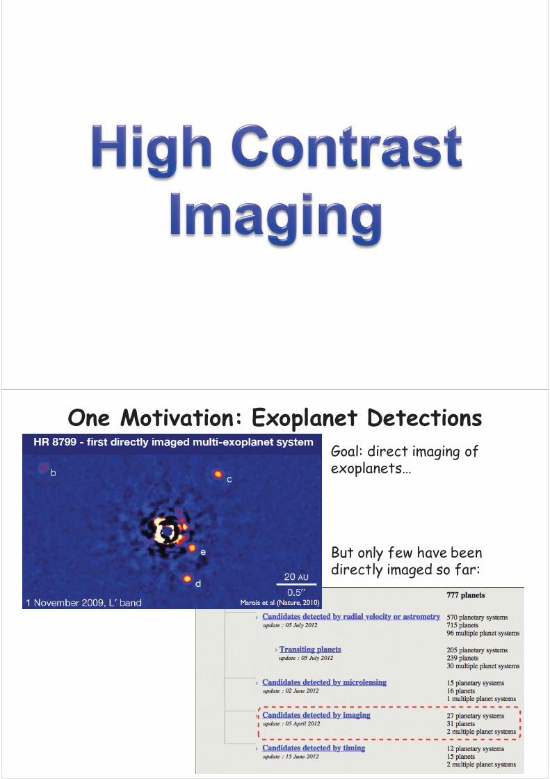
One Motivation: Exoplanet Detections Goal: direct imaging of exoplanets… But only few have been directly imaged so far:
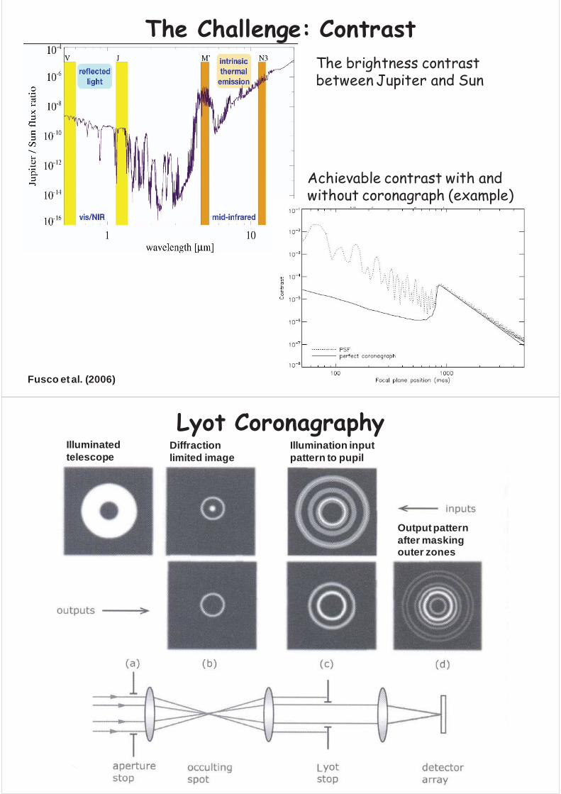
The Challenge: Contrast
Fusco et al. (2006)
The brightness contrast between Jupiter and Sun
Achievable contrast with and without coronagraph (example)
Lyot Coronagraphy Illuminated telescope
Diffraction limited image
Illumination input pattern to pupil
Output pattern after masking outer zones


![Astronomische Waarneemtechnieken (Astronomical ...brandl/OBSTECH/Handouts...Atmospheric Refraction 0 10 20 30 40 50 60 0 20406080 100 Atmospheric Refraction Zenith angle T [deg] Refraction](https://img.pdfslide.net/doc/110x75/5f21cfff831f4077a733bbd4/astronomische-waarneemtechnieken-astronomical-brandlobstechhandouts-atmospheric.jpg)