Approximate Dynamic Programming for Networks: Fluid Models

and Constraint Reduction

Michael H. Veatch

Department of Mathematics

Gordon College

mike.veatch@gordon.edu

August 19, 2009

Abstract

This paper demonstrates the feasibility of using approximate linear programming (ALP) to compute

nearly optimal average cost for multiclass queueing network control problems of moderate size. The

method requires only solving an LP and approximates the differential cost by a linear form. Quadratics,

certain exponential functions, piece-wise quadratic functions from fluid models, and other approximating

functions are used. The ALP is made more tractable for these three types of functions by algebraically

reducing the constraints to a smaller equivalent set. On examples with two to six buffers, bounds on

average cost were 12 to 40% below optimal using quadratic approximating functions; error was reduced

to 2 to 21% by using about twice as many approximating functions and can be reduced further by

systematically adding functions. Although the size of the LP is exponential in the number of buffers,

examples with up to 17 buffers and quadratic approximation are solved. For a given level of accuracy,

the method requries much less computation than standard value iteration. Policies are also constructed

from the ALP.

1 Introduction

The increasing size, complexity, and flexibility of manufacturing processes, supply chains, communications,

and computer systems have made them increasingly difficult to model and to operate efficiently. Recurrent

themes seen in many industries are a large number of interacting processes and significant randomness due

to customer demand which must be rapidly served, in addition to uncertainties in the service process. The

natural modeling framework for these systems is a multiclass queueing network (MQNET). Even under

the simplest assumptions of exponentially distributed service and interarrival times and linear holding costs,

MQNET control problems are NP-hard so that we cannot hope to solve large problems exactly [22]. Standard

policy iteration or value iteration are too computationally intensive to use even on moderate size problems,

particularly in heavy traffic, due to the well-known “curse of dimensionality.”

This paper demonstrates the feasibility of using approximate linear programming (ALP) to approximate

optimal average cost for MQNETs dramatically faster than exact dynamic programming (DP) methods.

1

A lower bound on optimal average cost could be very valuable for benchmarking the many heuristics for

controlling these systems. The justification of these heuristic policies has been less than satisfactory. Many

heuristic policies have been shown to be stable, but relatively little is known about suboptimality. Certain

policies have been shown to be asymptotically optimal for the limiting Brownian control problem in heavy

traffic or the fluid control problem, which essentially considers large buffer contents. However, asymptotic

optimality is generally too loose a criteria for designing near-optimal policies.

The main challenge in applying any approximate DP method, including ALP, is selecting a compact but

accurate class of approximating functions for the differential cost. The first contribution of this paper is

identifying new approximating functions that are shown numerically to improve accuracy. More specifically,

an improved trade-off between speed or size of the LP and accuracy is achieved. We begin with a quadratic

approximation, which has been used by several researchers, and test its speed and accuracy. A natural

refinement of the quadratic approximation is the “cost to drain” of the associated fluid model, which is

either quadratic or piece-wise quadratic. Fluid cost has been used to initialize the value iteration algorithm

[5]. In this paper we find and use these quadratic regions for a three-class example. We also use approximating

functions with certain exponential terms and indicator functions that aggregate states based on an estimate

of their importance to the approximation. These approximating functions are motivated by the problem

structure and numerical experience.

The second challenge in solving the ALP is that it contains one constraint for every state-action pair,

which is impractical for large networks. An open network with uncontrolled arrivals has an infinite state

space; truncating by limiting buffer sizes results in an ALP that is too large. Without some method of

reducing the number of constraints, the alternatives of approximate value iteration or approximate policy

iteration may be preferable. The second major contribution of this paper is to provide new constraint

reduction methods for piece-wise quadratic functions and certain exponential functions. We also use the

constraint reduction method in [20] for quadratic functions. For each type of function, the number of

constraints is still exponential in the number of buffers; however, the reduction extends considerably the size

of problem for which the ALP can be solved. The ALP approach also has the simplicity of just solving an

LP and the advantage of somewhat stronger theoretical results than for the other methods; see [7] and [25].

We also briefly addresses the policies associated with the differential cost approximations. The approx-

imation architectures are compact enough that one could implement these policies. However, testing has

shown that they do not always have good performance and may not even be stabilizing, as demonstrated

in [6] for a related control problem involving a single queue. We report some cases where the ALP gives

a useful policy. A final contribution involves upper bounds on average cost. An upper bound ALP for a

specific policy is given in [20]. We propose solving the lower bound ALP and using the associated policy in

the upper bound ALP. A second bound is derived that uses Bellman error.

Accuracy of the ALP bound was tested on networks with up to six buffers which could be solved using

value iteration. In general, accuracy improves as more basis functions are added to the approximation. The

quadratic approximation uses the smallest LP and gave an average cost 12 to 40% below optimal. When

exponential or piece-wise quadratic approximations were added, roughly doubling the number of variables,

accuracy improved to 2 to 21%. Adding indicator functions gradually achieved greater accuracy: for a two-

class series queue with traffic intensity of 0.8, an error of less than 1% was achieved using 113 functions,

including indicator functions for individual states. For a three-class reentrant line with a traffic intensity of

2

0.9, an error of 5% was achieved using 2309 functions. These LPs used dramatically fewer variables and less

time than is needed to achieve the same accuracy with value iteration. Speed of the ALP with quadratic

approximation was tested on larger examples, demonstrating that it can be solved on series lines with 17

buffers. Even larger multiclass networks could be solved, since they have fewer servers and control actions.

The ALP approach was originally proposed by [26]. It is applied to discounted network problems in [7]

using quadratic value function approximations. They provide an error bound for the ALP value function.

In particular, a suitable weighted norm of the error is bounded by the minimum of this error norm over all

functions in the approximating class, multiplied by a constant that does not depend on problem size. Similar

bounds are given on performance of the policy implied by the ALP value function. Instead of constraint

reduction, they use importance sampling of constraints, which is shown to be probabilistically accurate in [8].

For average cost problems, two modifications of the ALP approach are proposed in [6] and [9]. Although the

latter provides a performance bound, it is not clear how to apply it to networks. In [29], column generation

methods are used to solve average cost ALPs more efficiently. Approximate dynamic programming is applied

to a specific communication network—a crossbar switch—in [19] using “ridge” functions of a single variable

and to inventory problems in [1] and [28] using linear functions. We tested separable approximations, i.e.,

functions of a single buffer size, on several MQNETs and found that they were not as accurate as any of the

functions listed above—even quadratics. A major difference between our work and [19] is that we identify

different approximating functions which give a better trade-off between speed and accuracy for a test suite

of MQNETs.

The papers most closely related to ours are [20] and [21], which also consider average cost ALPs and

piece-wise quadratic approximations. Using a different quadratic on each set of states defined by which

buffers are empty, they reduce the constraints to a finite set. This set of approximating functions grows

exponentially with the number of buffers and is larger than the piece-wise quadratic approximation that

we propose. Our paper differs in that we use additional approximating functions, which are demonstrated

numerically to give tighter bounds, and the development of constraint reduction methods for more general

piece-wise quadratic and for certain exponential functions. Another difference is that they consider specific

controls, rather than bounding average cost for a class of controls.

Average cost bounds have also been obtained for queueing networks using the achievable region method

[4], [13] and Lyapunov functions [3]. These results are elegant but not very satisfactory from a numerical

viewpoint. For example, the achievable region bound is quite loose in balanced heavy traffic, i.e., when more

than one server has a traffic intensity near one. A duality relationship between the achievable region method

and certain ALPs with quadratic approximation is noted in [12]. This relationship leads to the result that

even the smallest, quadratic approximation ALP gives a tighter bound than the achievable region LP; see

[20, Appendix A] and [24].

The rest of this paper is organized as follows. Section 2 defines the MQNET sequencing problem and

the associated fluid control problem and Section 3 describes average cost ALPs. In Section 4 a variety of

approximations and their constraint reductions are presented, including detailed analysis of a series queue

and a reentrant line. Numerical results on the accuracy and speed of various ALPs are presented in Section

5. Some open questions are discussed in Section 6.

3

2 Open MQNET sequencing: Discrete and fluid models

In this section we describe the standard MQNET model and the fluid model associated with it. There are n

job classes and m resources, or stations, each of which serves one or more classes. Associated with each class

is a buffer in which jobs wait for processing. Let xi(t) be the number of class i jobs at time t, including any

that are being processed. Class i jobs are served by station σ(i). The topology of the network is described

by the routing matrix P = [pij], where pij is the probability that a job finishing service at class i will be

routed to class j, independent of all other history, and the m× n constituency matrix with entries Cji = 1

if station j serves class i and Cji = 0 otherwise. If routing is deterministic, then pi,s(i) = 1, where s(i) is the

successor of class i, and pp(i),i = 1,where p(i) as the predecessor of class i.

Exogenous arrivals occur at one or more classes according to independent Poisson processes with rate αi

in class i. Processing times are assumed to be independently exponentially distributed with mean mi = 1/µiin class i. To create an open MQNET, the routing matrix P is assumed to be transient, i.e., I+P +P 2+ . . .

is convergent. As a result, there will be a unique solution to the traffic equation

λ = α+ P ′λ

given by

λ = (I − P ′)−1α.

Here λi is the effective arrival rate to class i, including exogenous arrivals and routing from other classes,

and vectors are formed in the usual way. The traffic intensity is given by

ρ = C diag(m1, . . . ,mn)λ,

that is, ρj is the traffic intensity at station j. Stability requires that ρ < 1.

The network has sequencing control: each server must decide which job class to work on next, or possibly

to idle. Preemption is allowed. Let ui(t) = 1 if class i is served at time t and 0 otherwise. Admissible

controls are nonanticipating and have

Cu(t) ≤ 1

ui(t) ≤ xi(t).

The first constraint states that a server’s allocations cannot exceed one; the second prevents serving an

empty buffer.

The objective is to minimize long-run average cost

J(x, u) = lim supT→∞

1

TEx,u

∫ T

0

c′x(t)dt.

Here Ex,u denotes expectation given the initial state x(0) = x and policy u. Consider only stationary Markov

policies and write u(t) = u(x(t)). We use the uniformized, discrete-time Markov chain and assume that the

4

potential event rate is∑ni=1(αi + µi) = 1. Let Pu = [pu(x, y)] be the transition probability matrix under

policy u and use the notation

(Puh)(x) =∑

y

pu(x, y)h(y).

Due to the linearity of Pu with respect to u, only extreme points ui = 0 and ui = 1 need be considered. Let

A(x) be the set of feasible extreme point controls in state x and A be their union.

Under the condition ρ < 1, the control problem has several desirable properties:

1. An optimal policy exists and its average cost is constant, J∗ = minu J(x, u) for all x.

2. There is a solution J∗ and h∗ to the average cost optimality equation

J + h(x) = c′x+ minu∈A(x)

(Puh)(x). (1)

3. Under the additional condition that h is bounded below by a constant and above by a quadratic, there

is a unique solution J∗ and h∗ to (1) satisfying h∗(0) = 0. Furthermore, J∗ is the optimal average cost,

any policy

u∗(x) = arg minu∈A(x)

(Puh∗)(x)

is optimal, and h∗ is the differential cost of this policy,

h∗(x) = lim supT→∞

(Ex,u∗

∫ T

0

c′x(t)dt−E0,u∗

∫ T

0

c′x(t)dt

). (2)

Properties (1) and (2) can be established using general results for MDPs as in [27, Theorems 7.2.3 and 7.5.6].

For networks, properties (1) and (2) are shown in [15, Theorem 7]; (3) is obtained by applying standard

verification theorems to networks; see, e.g., [14, Theorem 2.1 and Section 7] and [16, Theorem 10.7].

A natural starting point in approximating the differential cost function is the associated fluid model. In

this model all transitions are replaced by their mean rates and a continuous state qi(t) ∈ R+ is used. In a

fluid control problem, for each initial state there is a time horizon T such that q(t) = 0 for all t ≥ T . The

fluid control problem corresponding to (1) is

(FCP) V (x) = min

∫ T

0

c′q(t)dt

q(t) = Bu(t) + α

Cu(t) ≤ 1

q(0) = x

q(t) ≥ 0, u(t) ≥ 0,

where α = (α1, . . . , αn)′and B = (P ′− I)diag(µ1, . . . .µn). An optimal u(t) can be chosen so that it is piece-

wise constant, making q(t) piece-wise linear with q(t) existing except on a set of zero measure. We will use

the fluid “cost to drain” V (x) to guide our approximation of h(x). The motivation for this approximation is

5

[15, Theorem 7(iv)], based on [14, Theorem 5.2]. It establishes the following connection between the discrete

and fluid cost functions:

limθ→∞

h∗(θx)

V (θx)= 1, (3)

i.e., the differential cost is dominated by the fluid cost as queue lengths increase; see [31] for discussion of

the policy implications.

The fluid cost V is also piece-wise quadratic and C1. The quadratic regions depend on the optimal fluid

policy u(x), which partitions Rn+ into a finite number of control switching sets where the control is constant.

Each switching set is a convex polyhedral cone emanating from the origin. In particular, if a switching set

contains x, it also contains θx, θ > 0. Switching sets can be subdivided according to the (finite) sequence of

switching sets that a trajectory enters next. In a region, say Sk, where a certain sequence of switching sets

will be visited, V is quadratic and we write

V (x) =1

2x′Qkx, x ∈ Sk. (4)

Thus, (3) implies that

h∗(x) =1

2x′Qkx+ o(|x|2), x ∈ Sk. (5)

Fundamentally, V is quadratic in these regions because q(t) is constant in a switching set, so that the

integrand in (FCP) is piece-wise linear.

3 Approximate LP: Average cost bounds

In this section we describe a general method for constructing a linear program in a small number of variables

that approximates the differential cost and places a lower bound on average cost. It is well-known that,

for finite state spaces, an inequality relaxation of Bellman’s equation gives an equivalent LP in the same

variables,

(LP) max J

s.t. J + h(x) ≤ c′x+ (Puh)(x) for all x ∈ Zn+, u ∈ A(x)

h(0) = 0.

An additional condition on h is needed because of the countable space: For some L1, L2 > 0,

−L1 ≤ h(x) ≤ L2(1 + |x|2). (6)

Appendix A shows that (1) is equivalent to (LP) and (6). This exact LP has one variable for every state.

To create a tractable LP, the differential cost can be approximated by a linear form

h∗(x) ≈K∑

k=1

rkφk(x) = (Φr)(x) (7)

using some small set of basis functions φk and variables rk. Assume that φk(0) = 0. The resulting approxi-

6

mate LP is

(ALP) J =max J

s.t. J + (Φr)(x) ≤ c′x+ (PuΦr)(x) for all x ∈ Zn+, u ∈ A(x)

− L1 ≤ (Φr)(x) ≤ L2(1 + |x|2) for all x ∈ Zn+.

The bounds L1 and L2 may depend on r; all that is needed is that the bound applies to each φk. Since

(ALP) is equivalent to the exact LP with the constraints (7) added, the exact LP is a relaxation. Hence,

(ALP) gives a lower bound, J∗ ≥ J . (ALP) is feasible, so it has an optimal solution, say r∗.

To compute an upper bound, one must identify a policy or set of policies. Of course, a policy u can be

simulated to estimate its average cost Ju. Alternatively, the following upper bound ALP can be used:

(ALPUB) J =min J

s.t. J + (Φr)(x) ≥ c′x+ (PuΦr)(x) for all x ∈ Zn+

− L1 ≤ (Φr)(x) ≤ L2(1 + |x|2) for all x ∈ Zn+.

Then J ≥ Ju ≥ J∗. Note that in addition to reversing the inequality in (ALP) and minimizing, (ALPUB)

considers a single policy. Including constraints for a class of policies, e.g., nonidling, is used to check stability.

Any differential cost approximation h defines an h-greedy policy

uh(x) = arg minu∈A(x)

(Puh)(x).

The approximation architecture Φ restricts the greedy policy to a certain class of policies. For example, a

quadratic approximation architecture implies linear boundaries between control regions. The greedy policy

from (ALP) may have poor performance or not even be stabilizing. However, in some cases it has good

performance, so we use it in (ALPUB) to construct an upper bound on average cost.

The numerical tests in Section 5 use (ALP) and (ALPUB). However, after solving (ALP) another approach

to an upper bound is to use Bellman error, defined for any J and h as

B(x) = minu∈A(x)

(Puh) (x)− h (x) + c′x− J

= (Puh) (x)− h (x) + c′x− J

= [(Pu − I)h](x) + c′x− J,

where u is an h-greedy policy. If J, h satisfy the constraints (ALP) then B(x) ≥ 0 is the minimum slack

of constraints for that x. Under the assumption that the h-greedy policy is stabilizing, we can bound the

average cost error J − J∗ using Bellman error.

Proposition 1 Let J, r be feasible for (ALP), h = Φr, and u be an h-greedy policy. Assume

A1. u is stabilizing. Let Eu denote expectation with respect to a stationary distribution for policy u.

A2. Ju <∞ and Eu(B) <∞.

7

Then

J∗ − J = (J∗ − Ju) +Eu(B) ≥ Eu(B). (8)

Proof. By the definition of B,

J + h(x) = c′x−B(x) + minu∈A(x)

(Puh)(x),

so J, h satisfy (1) for the perturbed problem with cost c′x−B(x). Since (ALP) includes the growth condition

(6), J is the average cost for this problem under policy u:

J = Eu[c′x−B(x)] = Ju −E

u(B)

which implies (8).

To compute the expectation in (8) one could simulate the policy u. The term in parentheses is the

suboptimality of policy u. ALP policies can be unstable or have large suboptimalities, so the bound will not

be useful in all examples. Other error bounds are proposed in [6] and [9] for variants of the ALP approach.

The quadratic bound on h (6) implies that, at least for sufficiently smooth h, Bellman error is bounded

by a linear function. The precise form of B for quadratic h is shown in Section 4.1. A linear bound also

holds for the other approximation architectures that we propose; the fundamental reason is that B depends

on h only through the differences h(x + ei) − h(x), where ei is a unit vector with ith component equal to

1. A linear bound on h has the advantage that the assumption Eu(B) <∞ in Proposition 1 is no stronger

than Ju <∞.

If the approximation architecture happens to include the exact differential cost, (ALP) will find it.

Proposition 2 If either h∗ = Φr for some r or (ALP) has a binding constraint for each state x then

(i) J∗ = J and h∗ = Φr∗.

(ii) If {φk} are linearly independent on Zn+, then (ALP) has a unique optimal solution.

Proof. Suppose h∗ = Φr. Then J∗ and Φr satisfy (1) and are optimal for (ALP). By assumption, (Φr∗)(0) =

0 and uniqueness of solutions to (1) implies that J∗ and r are the unique optimal solution to (ALP), i.e.,

r∗ = r and (i) holds.

Now suppose (ALP) has a binding constraint for each state. Then J and Φr∗ satisfy (1) for each x, with

the minimum achieved by the action u(x) with the binding constraint in (ALP), again implying (i). (ii)

follows easily from (i).

The approximate LP is still not a manageable size because it has one constraint for each state-action

pair. In Section 4, various constraint sets are algebraically reduced or approximated by a smaller set of

constraints.

4 Differential cost approximation and constraint reduction

This section considers several bases Φ to approximate the differential cost and demonstrates how the con-

straints of the resulting ALP can be algebraically reduced to a small, or at least more easily approximated,

8

set. In Section 4.1, constraint reduction is given for quadratic approximation. Section 4.2 introduces ex-

ponential approximating functions and a method of reducing the constraints, using a series queue as an

example. A method of reducing piece-wise quadratic approximations, which are suggested by fluid models,

is presented in Section 4.3. A larger class of indicator functions is proposed in Section 4.4.

4.1 Quadratic approximation

Consider the quadratic differential cost approximation

h(x) =1

2x′Qx+ px (9)

where Q = [qij ] is symmetric. This approximation is motivated by (5). It is also interesting to note that for

a single uncontrolled queue

h∗(x) =1

2(µ− α)(x2 + x). (10)

The quadratic term in (10) matches the fluid value function; the effect of randomness is to shift the fluid

value function 1/2 unit to the left.

The constraints (ALP) can be reduced to a finite set for quadratic h [20, Appendix A]. To simplify

notation, consider only deterministic routing. First, we write the constraints as

J ≤n∑

i=1

(cixi + αi[h(x+ ei)− h(x)] + uiµi[h(x− ei + es(i))− h(x)]) for all x ∈ Zn+, u ∈ A(x). (11)

Unlike a discounted model, only differences in h appear in these constraints, simplifying the analysis. It is

convenient to let x = z + u, so that a control u is feasible for all z ∈ Zn+. Substituting (9) into (11) yields

J ≤ du + cu′z for all z ∈ Zn+, u ∈ A (12)

where

cui = ci +n∑

j=1

[αjqij + ujµj(qi,s(j) − qij)]

du =n∑

i=1

[ui(cui + µi(

1

2qii +

1

2qs(i),s(i) − qi,s(i) + ps(i) − pi)) + αi(

1

2qii + pi)]

and cu = [cui ]. For (12) to hold for all z, the right hand side must be nondecreasing in zi. Hence, (12) is

equivalent to

J ≤ du (13)

cui ≥ 0 for i = 1, . . . , n, u ∈ A (14)

9

If the optimal policy is nonidling, then for a given control u, (14) is only needed for i in

N(u) =

i :

∑

j:σ(i)=σ(j)

uj = 1

,

i.e., the classes served by busy stations. Under nonidling there are only |N(u)| + 1 constraints for each u

instead of n+ 1.

The number of constraints in (13) and (14) is typically exponential in n because of the number of actions

|A|. Nevertheless, the reduced ALP is small enough to solve for moderate n.

For quadratic h, Bellman error has the form

B(x) = minu∈A(x)

du + (cu)′(x− u)− J,

which is the minimum of linear functions.

4.2 Exponential approximations and a series queue

Although quadratic approximation architectures are efficient, the error in average cost is often fairly large as

shown in Section 5. In this section we introduce exponential approximating functions for a general network.

A more detailed analysis, with constraint reduction, is given for a series queue.

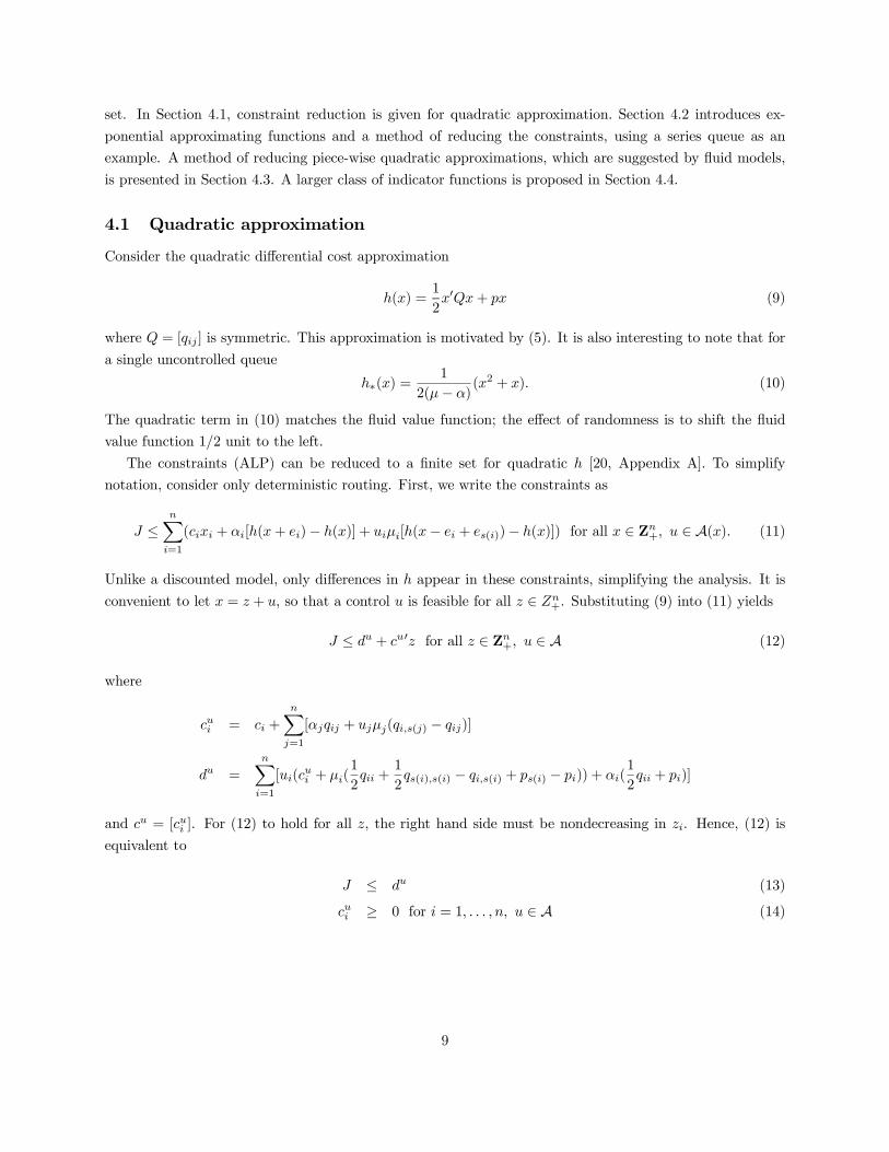
Numerical experience suggests that a quadratic approximation misses important features of h∗ in states

where certain queue lengths are small or zero. Figure 1 shows the residual when a quadratic is fit to h∗ over

the region graphed for the series queue with µ1 > µ2 of Section 5. The residuals, plotted on the z axis, are

small compared to h∗; the largest value of h∗ on this grid is over 500. The percent residual is larger when x is

small and particularly when x2 is small. The optimal stationary distribution also has larger probabilities in

these states. In fact, above a switching curve where server 1 idles the probabilities are zero. In this example,

the switching curve limits x2 ≤ 5 when x1 = 1 and x2 ≤ 9 when x1 = 10. Thus, additional functions to

approximate the complex shape of h∗ when x2 is small appear important.

For general networks, to emphasize states with small xi, we will use the function

φi (x) = βxii , (15)

where βi < 1. There is a natural choice of β for some classes. If class i has a predecessor class, no arrivals,

and µp(i) > µi set β = µi/µp(i). Then

[(Pu − I)φi] (x) =[(αi + up(i)µp(i))(βi − 1) + uiµi(1/βi − 1)

]φi(x)

=[up(i)µp(i))(µi/µp(i) − 1) + uiµi(µp(i)/µi − 1)

]φi(x) (16)

= (up(i) − ui)(µi − µp(i))φi(x).

Note that if the two classes have different servers, σ(p(i)) = σ(i), then in states where both are being served,

up(i) = ui = 1 and (16) is equal to 0, i.e., (16) is in the kernel of the generator Pu. This has two advantages.

First, as shown below, it allows constraint reduction. Second, it can influence Bellman error in states where

10

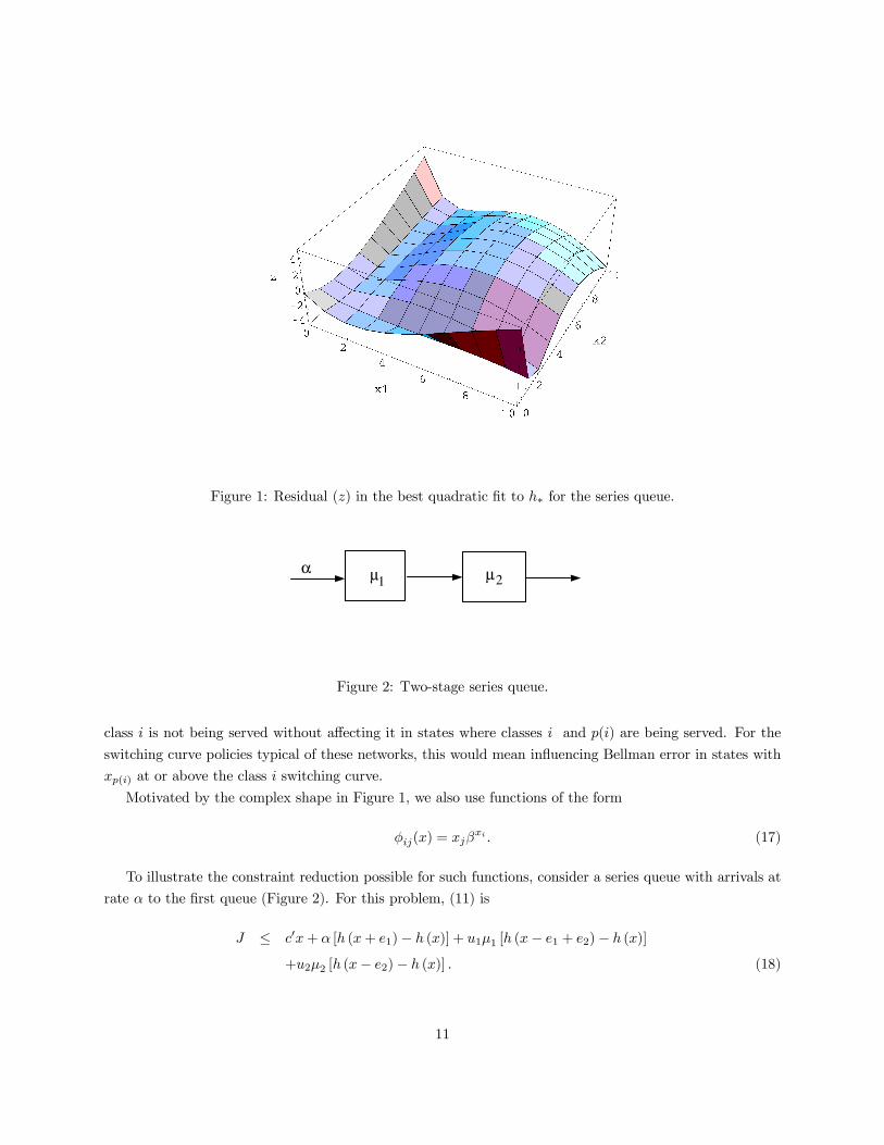
Figure 1: Residual (z) in the best quadratic fit to h∗ for the series queue.

α µ 1 µ 2

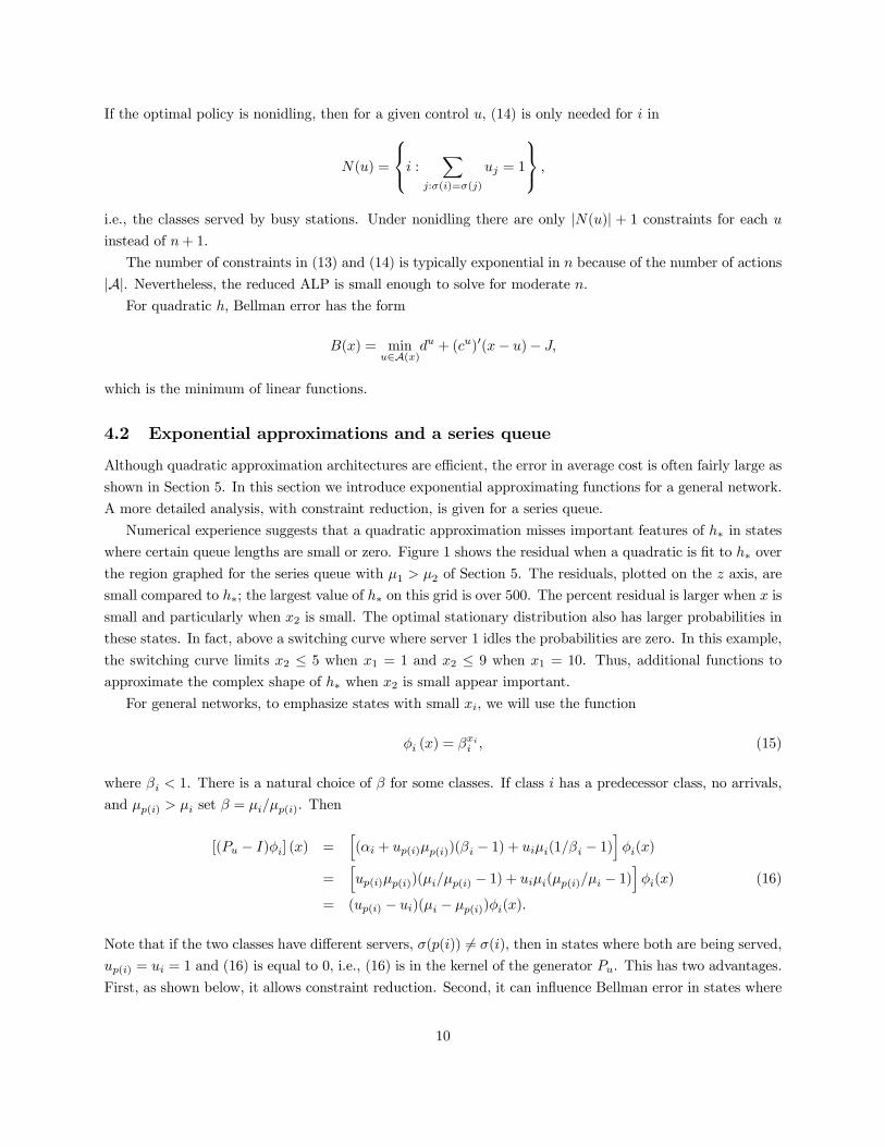
Figure 2: Two-stage series queue.

class i is not being served without affecting it in states where classes i and p(i) are being served. For the

switching curve policies typical of these networks, this would mean influencing Bellman error in states with

xp(i) at or above the class i switching curve.

Motivated by the complex shape in Figure 1, we also use functions of the form

φij(x) = xjβxi . (17)

To illustrate the constraint reduction possible for such functions, consider a series queue with arrivals at

rate α to the first queue (Figure 2). For this problem, (11) is

J ≤ c′x+ α [h (x+ e1)− h (x)] + u1µ1 [h (x− e1 + e2)− h (x)]

+u2µ2 [h (x− e2)− h (x)] . (18)

11

We consider the case c1 < c2, so that station 1 might idle (station 2 is always nonidling), and α < µ2 ≤ µ1,

so that the fluid policy is greedy: idle 1 when x2 > 0 [2]. Use the approximation

h(x) =1

2x′Qx+ px+ r1φ2(x) + r2φ21(x) + r3φ22(x) (19)

i.e., the functions (15) and (17) with i = 2 are added to the quadratic. Set β ≡ β2 = (µ2/µ1). Substituting

(19) into (18) and again using x = z + u, (18) has the form

J ≤ du + cu′z + (ζu + ξu′z)βz2+u2 (20)

for all z ∈ Z2+ and all u that are nonidling at station 2. Here du, cu, ζu and ξu are linear functions of the

variables p, Q, and r; see Appendix B. For u = (1, 1), ξ(1,1) = 0, so as zi →∞ we must have

c(1,1)i ≥ 0, i = 1, 2. (21)

Given (21), (20) is tightest at z1 = 0 for each z2. However, depending on the value of ζ((1,1) it could be

tightest at any z2. Thus, we will approximate (ALP) by including (20) at z1 = 0, z2 = 0, . . . , N − 1 for some

N . Now consider u = (0, 1). For each z2, the z1 coefficient must be nonnegative,

c(0,1)1 + βξ

(0,1)1 βz2 ≥ 0.

Because of the monotonicity in z2, this is equivalent to

c(0,1)1 + βξ

(0,1)1 ≥ 0 (22)

and c(0,1)1 ≥ 0. Letting z2 →∞ in (20) gives another constraint, so we have

c(0,1)i ≥ 0, i = 1, 2. (23)

Given (22) and (23), (20) is tightest at z1 = 0 but, depending on ζ(0,1) and ξ(0,1)2 , could be tightest at any

z2, so we include (20) at u = (0, 1), z1 = 0, and z2 = 0, . . . , N − 1. Next, for u = (1, 0) we must have z2 = 0.

For (20) to hold as z1 →∞, we must have

c(1,0)1 ≥ 0. (24)

In light of (24), (20) is tightest at z1 = 0, so we include (20) at u = (1, 0) and z = (0, 0). Finally, we include

(20) at u = z = (0, 0).

To summarize, the approximate reduced ALP contains the 2N +8 constraints (20) at u = (1, 1), z1 = 0,

z2 = 0, . . . , N − 1; u = (0, 1), z1 = 0, z2 = 0, . . . , N − 1; u = (1, 0), z = (0, 0); and u = z = 0; plus (21)-(24).

Call this relaxation ALP(N). The following proposition shows that ALP(N) is exact for some N . In practice,

a quite small N is usually sufficient.

Proposition 3 Let JN be the optimal value of ALP(N) for the series queue. For some M , JN = J for all

N ≥M .

The proposition follows from the fact that the limiting constraints as x2 → ∞, namely, (21)-(24), are

12

µ1

µ3

µ 2

α1

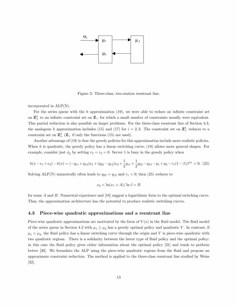
Figure 3: Three-class, two-station reentrant line.

incorporated in ALP(N).

For the series queue with the h approximation (19), we were able to reduce an infinite constraint set

on Z2+ to an infinite constraint set on Z+ for which a small number of constraints usually were equivalent.

This partial reduction is also possible on larger problems. For the three-class reentrant line of Section 4.3,

the analogous h approximation includes (15) and (17) for i = 2, 3. The constraint set on Z3+ reduces to a

constraint set on Z2+ (Z+ if only the functions (15) are used).

Another advantage of (19) is that the greedy policies for this approximation include more realistic policies.

When h is quadratic, the greedy policy has a linear switching curve; (19) allows more general shapes. For

example, consider just φ2 by setting r2 = r3 = 0. Server 1 is busy in the greedy policy when

h(x− e1+ e2)−h(x) = (−q11+q12)x1+(q22− q12)x2+1

2q11+

1

2q22− q12−p1+p2− r1(1−β)βx2 < 0. (25)

Solving ALP(N) numerically often leads to q22 = q12 and r1 < 0; then (25) reduces to

x2 < ln(x1 +A)/ lnβ +B

for some A and B. Numerical experience and [18] suggest a logarithmic form to the optimal switching curve.

Thus, the approximation architecture has the potential to produce realistic switching curves.

4.3 Piece-wise quadratic approximations and a reentrant line

Piece-wise quadratic approximations are motivated by the form of V (x) in the fluid model. The fluid model

of the series queue in Section 4.2 with µ1 ≥ µ2 has a greedy optimal policy and quadratic V . In contrast, if

µ1 < µ2, the fluid policy has a linear switching curve through the origin and V is piece-wise quadratic with

two quadratic regions. There is a solidarity between the latter type of fluid policy and the optimal policy:

in this case the fluid policy gives richer information about the optimal policy [31] and tends to perform

better [30]. We formulate the ALP using the piece-wise quadratic regions from the fluid and propose an

approximate constraint reduction. The method is applied to the three-class reentrant line studied by Weiss

[32].

13

Control region visited nextQuadratic region (x > 0) State Station 1 serves q

S1 : x3 > γx1 +αγ+µ

3−µ

2

µ2

x2 x2 = 0, x3 > γx1 3 (α, 0, µ2 − µ3)

S2 : x3 ≤ γx1 +αγ+µ

3−µ

2

µ2

x2 x2 = 0, x3 ≤ γx1 1 and 3 (α− µ2, 0, µ2 − µ3(1−µ2

µ1

))

and x3 >µ3−µ

2

µ2

x2

S3 : x3 ≤µ3−µ

2

µ2

x2 x2 > 0, x3 = 0 3 and idle (α,−µ2, 0)

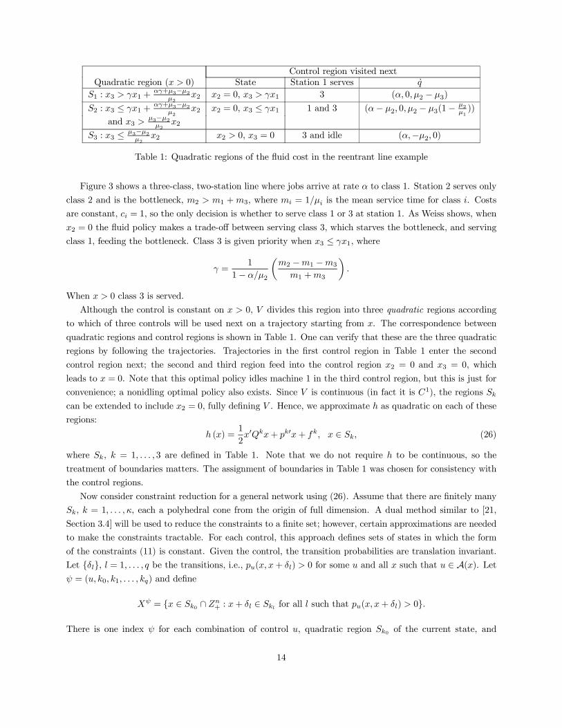
Table 1: Quadratic regions of the fluid cost in the reentrant line example

Figure 3 shows a three-class, two-station line where jobs arrive at rate α to class 1. Station 2 serves only

class 2 and is the bottleneck, m2 > m1 +m3, where mi = 1/µi is the mean service time for class i. Costs

are constant, ci = 1, so the only decision is whether to serve class 1 or 3 at station 1. As Weiss shows, when

x2 = 0 the fluid policy makes a trade-off between serving class 3, which starves the bottleneck, and serving

class 1, feeding the bottleneck. Class 3 is given priority when x3 ≤ γx1, where

γ =1

1− α/µ2

(m2 −m1 −m3

m1 +m3

).

When x > 0 class 3 is served.

Although the control is constant on x > 0, V divides this region into three quadratic regions according

to which of three controls will be used next on a trajectory starting from x. The correspondence between

quadratic regions and control regions is shown in Table 1. One can verify that these are the three quadratic

regions by following the trajectories. Trajectories in the first control region in Table 1 enter the second

control region next; the second and third region feed into the control region x2 = 0 and x3 = 0, which

leads to x = 0. Note that this optimal policy idles machine 1 in the third control region, but this is just for

convenience; a nonidling optimal policy also exists. Since V is continuous (in fact it is C1), the regions Sk

can be extended to include x2 = 0, fully defining V . Hence, we approximate h as quadratic on each of these

regions:

h (x) =1

2x′Qkx+ pk′x+ fk, x ∈ Sk, (26)

where Sk, k = 1, . . . , 3 are defined in Table 1. Note that we do not require h to be continuous, so the

treatment of boundaries matters. The assignment of boundaries in Table 1 was chosen for consistency with

the control regions.

Now consider constraint reduction for a general network using (26). Assume that there are finitely many

Sk, k = 1, . . . , κ, each a polyhedral cone from the origin of full dimension. A dual method similar to [21,

Section 3.4] will be used to reduce the constraints to a finite set; however, certain approximations are needed

to make the constraints tractable. For each control, this approach defines sets of states in which the form

of the constraints (11) is constant. Given the control, the transition probabilities are translation invariant.

Let {δl}, l = 1, . . . , q be the transitions, i.e., pu(x, x+ δl) > 0 for some u and all x such that u ∈ A(x). Let

ψ = (u, k0, k1, . . . , kq) and define

Xψ = {x ∈ Sk0 ∩ Zn+ : x+ δl ∈ Skl for all l such that pu(x, x+ δl) > 0}.

There is one index ψ for each combination of control u, quadratic region Sk0 of the current state, and

14

quadratic region Skl of possible next states. If transition δl does not occur under u, then kl = k0.

To illustrate these definitions in the reentrant line example, number the service transitions l = 1, 2, 3 and

the arrival transition l = 4. Consider, for example, u = (0, 1, 1) and k0 = 3, i.e., x ∈ S3 (see Table 1). Then

k1 = 3 because class 1 is not served and k3 = k4 = 3 because these transitions cannot leave S3. However, a

class 2 service completion could stay in S3 (k2 = 3), enter S2 (k2 = 2), or, for certain parameter values, enter

S1 (k2 = 1). Specifically, if µ3 ≥ 2µ2 and x = (0, 1, 1) then x ∈ S3 but x+ δ2 = (0, 0, 2) ∈ S1, i.e., x ∈ Xψ

where ψ = (u, 3, 3, 1, 3, 3). Because S1 and S3 only meet at the origin, Xψ can contain only states near the

origin. In general, if ψ contains kl = k0 then Xψ lies within one transition of the hyperplane separating Sk0and Skl .

Again using x = z + u, let Zψ = {z : z + u ∈ Xψ}. The constraints have the form

J ≤ dψ + cψ′z +1

2z′Mψz, z ∈ Zψ (27)

where dψ, cψ, and Mψ are linear functions of Qk, pk, and fk. The quadratic term Mψ is symmetric.

It appears because of transitions between regions Sk. The first approximation is to remove the integer

restriction by allowing z ∈ Zψ

, where Zψ

is a polyhedron, say {z ∈ Rn : Aψz ≥ bψ, z ≥ 0}, whose lattice

points are (nearly) the set Zψ. For simplicity, we allow lattice points on the boundary of Zψ

that are not in

Zψ. This overlap could be avoided by adding more cutting planes. Also, because Sk has full dimension and

the control u is feasible at all z ≥ 0, there is no need for equality constraints in Zψ

. If nonidling controls

are desired, constraints of the form zi = 0 can be enforced by removing these variables.

Checking (27) exactly for a given dψ, cψ, and Mψ is related to determining if Mψ is copositive; instead,

following [21], we impose the stronger, simpler conditions

Mψ ≥ 0 (28)

and

J ≤ dψ + cψ′z

Aψz ≥ bψ (29)

z ≥ 0.

The key observation is that these constraints are colinear in z and the ALP variables. A dual can be

constructed that separates z. Fixed values of J , Qk, pk, and fk satisfy (29) if and only if, for each ψ, the LP

min cψ′z

s.t. Aψz ≥ bψ

z ≥ 0

15

has optimal value wψ ≥ J − dψ, or equivalently, so does its dual

max bψ′yψ

s.t. Aψ′yψ ≤ cψ (30)

yψ ≥ 0.

Thus, (30) and wψ ≥ J − dψ for all ψ are equivalent to (29). Reintroducing J , Qk, pk, and fk as variables,

the dual form of (ALP) is

(ALPD) max J

s.t. Aψ′yψ ≤ cψ

bψ′yψ ≥ J − dψ

Mψ ≥ 0

yψ ≥ 0.

The two approximations made were restrictions of (ALP); hence, the optimal value JD of (ALPD) is also a

lower bound, JD ≤ J∗.

(ALPD) has roughly n2/2 constraints for each ψ. It contains the roughly κn2/2 variables in (26) (recall

that κ is the number of quadratic regions) plus one dual variable for each constraint used to define the

polyhedra Zψ

. Both κ and the number of dual variables are generally exponential in n, but the latter

grows much more quickly due to the large number of regions indexed by ψ. Hence, (ALPD) has many more

variables than (ALP). We propose two reductions. First, if nonidling is assumed, then zi = 0 for i /∈ N(u),

and these zi can be eliminated before forming the dual.

Second, (29) can be interpreted geometrically as checking J ≤ dψ + cψ′z for every extreme point z and

cψ′β ≥ 0 for every extreme direction β of Zψ

. Because the hyperplanes bounding each Sk pass through the

origin, the ones bounding Zψ

pass within roughly one transition of the origin (there are points in Zψ within

one transition of the Sk boundary). Thus, in a certain sense, the extreme points of Zψ

lie near the origin.

Also, finding the extreme directions is made easier by the fact that the extreme directions of Zψ

are a subset

of the extreme directions of Sk0 . In particular, Zψ

has the ones contained in the common boundary of Sk0and all Skl (because there are transitions into Skl from Z

ψ). The extreme directions for the example in this

section are listed in Table 2. Checking extreme directions in the linear constraints (29) is an exact method;

however, we will apply it as an approximate check of (27). Requiring (27) at z = tβ for all t ≥ 0 results in

quadratic constraints. For simplicity, we use the stronger conditions cψ′β ≥ 0 and β′Mψβ ≥ 0.

These observations suggest the following approximation to (27). Find the extreme directions {βψ,l} of

Zψ

. The relaxation ALP(N) contains the constraints

(27) for z ∈ Zψ and zi ≤ N − 1

cψ′βψ,l ≥ 0 (31)

(βψ,l)′Mψβψ,l ≥ 0 (32)

16

Region Extreme directionsS1 (0, 0, 1), (0, µ2, αγ + µ3 − µ2), (1, 0, γ)S2 (1, 0, 0), (0, µ2, αγ + µ3 − µ2), (1, 0, γ), (0, µ2, µ3 − µ2)S3 (1, 0, 0), (0, 1, 0) (0, µ2, αγ + µ3 − µ2)

Table 2: Edges of the quadratic regions in the reentrant line example

for all ψ and all directions βψ,l. The constraints (27) address the extreme points, while the limiting constraints

(31) and (32) in the extreme directions allow faster convergence over N . ALP(N) has two limiting constraints

for every extreme direction βψ,l, which is generally exponential in n, plus Nn constraints (27). However, it

avoids the dual variables yψ, making it potentially more tractable than (ALPD).

Notice that ALP(N) is based on the exact constraints, not the linearization (29), suggesting that ALP(N)

might give a tighter bound than (ALPD). However, because of the approximate treatment of limiting con-

straints ALP(N) may not converge to (ALP).

In this example, the fluid policy and quadratic regions were determined analytically. For larger problems,

finding the fluid policy becomes intractable. An alternative is to analyze the two-station fluid workload

relaxation in [17], for which an optimal policy can easily be found. A “greedy, workload constrained”

translation of this policy from the workload space to the original state space is also given in [17]. It appears

that the quadratic regions for this policy could be determined algorithmically by working backward from the

origin and determining all sequences of control regions that can be visited, though we have not done so.

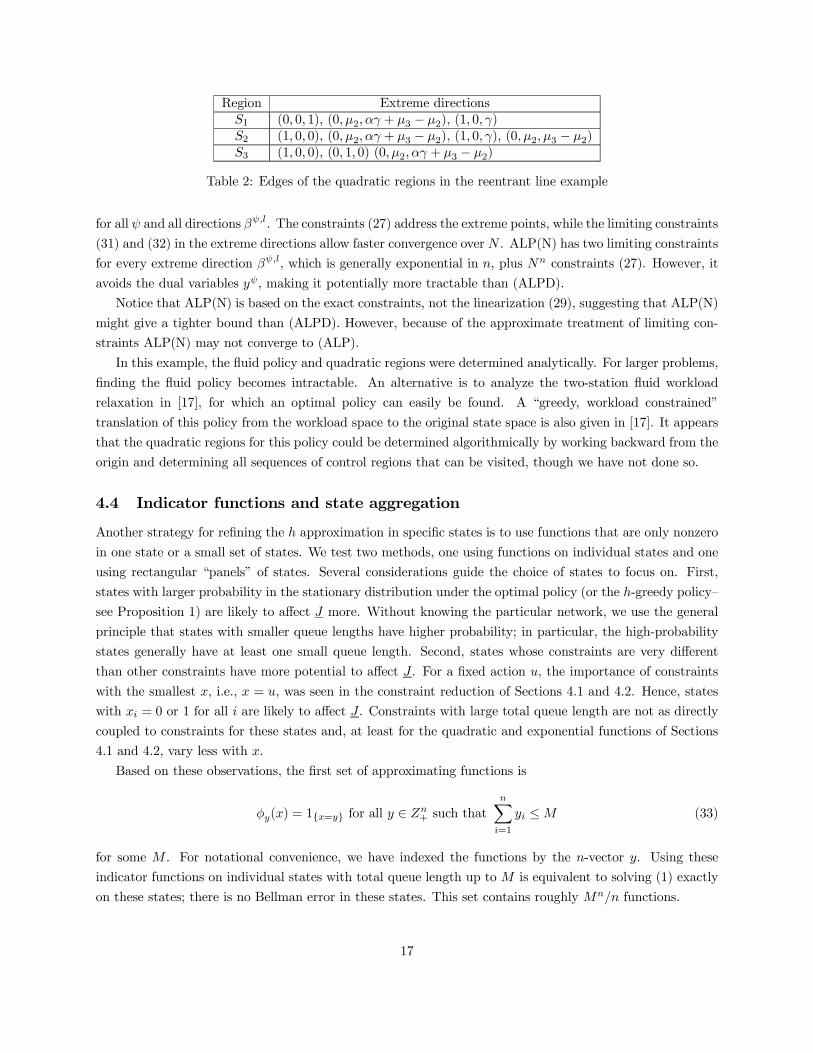
4.4 Indicator functions and state aggregation

Another strategy for refining the h approximation in specific states is to use functions that are only nonzero

in one state or a small set of states. We test two methods, one using functions on individual states and one

using rectangular “panels” of states. Several considerations guide the choice of states to focus on. First,

states with larger probability in the stationary distribution under the optimal policy (or the h-greedy policy—

see Proposition 1) are likely to affect J more. Without knowing the particular network, we use the general

principle that states with smaller queue lengths have higher probability; in particular, the high-probability

states generally have at least one small queue length. Second, states whose constraints are very different

than other constraints have more potential to affect J . For a fixed action u, the importance of constraints

with the smallest x, i.e., x = u, was seen in the constraint reduction of Sections 4.1 and 4.2. Hence, states

with xi = 0 or 1 for all i are likely to affect J . Constraints with large total queue length are not as directly

coupled to constraints for these states and, at least for the quadratic and exponential functions of Sections

4.1 and 4.2, vary less with x.

Based on these observations, the first set of approximating functions is

φy(x) = 1{x=y} for all y ∈ Zn+ such thatn∑

i=1

yi ≤M (33)

for some M . For notational convenience, we have indexed the functions by the n-vector y. Using these

indicator functions on individual states with total queue length up to M is equivalent to solving (1) exactly

on these states; there is no Bellman error in these states. This set contains roughly Mn/n functions.

17

µ1

µ4

µ 2

α1

α3 µ 3

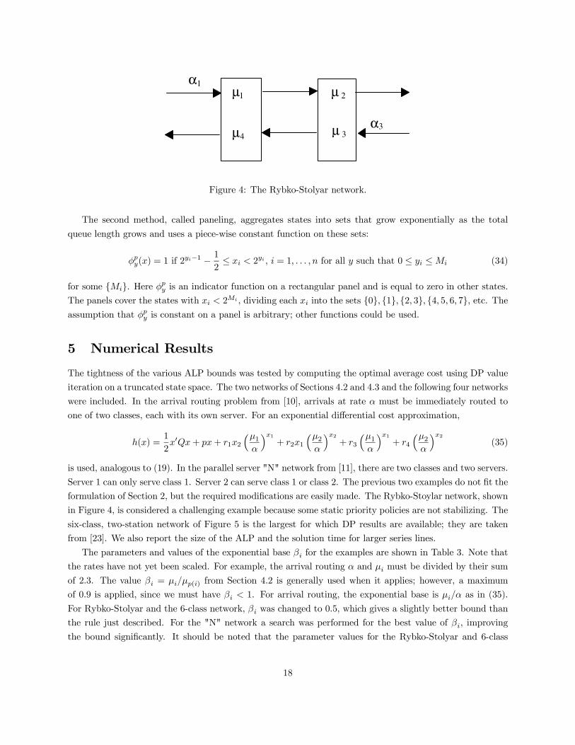
Figure 4: The Rybko-Stolyar network.

The second method, called paneling, aggregates states into sets that grow exponentially as the total

queue length grows and uses a piece-wise constant function on these sets:

φpy(x) = 1 if 2yi−1 −1

2≤ xi < 2

yi , i = 1, . . . , n for all y such that 0 ≤ yi ≤Mi (34)

for some {Mi}. Here φpy is an indicator function on a rectangular panel and is equal to zero in other states.

The panels cover the states with xi < 2Mi , dividing each xi into the sets {0}, {1}, {2, 3}, {4, 5, 6, 7}, etc. The

assumption that φpy is constant on a panel is arbitrary; other functions could be used.

5 Numerical Results

The tightness of the various ALP bounds was tested by computing the optimal average cost using DP value

iteration on a truncated state space. The two networks of Sections 4.2 and 4.3 and the following four networks

were included. In the arrival routing problem from [10], arrivals at rate α must be immediately routed to

one of two classes, each with its own server. For an exponential differential cost approximation,

h(x) =1

2x′Qx+ px+ r1x2

(µ1α

)x1+ r2x1

(µ2α

)x2+ r3

(µ1α

)x1+ r4

(µ2α

)x2(35)

is used, analogous to (19). In the parallel server "N" network from [11], there are two classes and two servers.

Server 1 can only serve class 1. Server 2 can serve class 1 or class 2. The previous two examples do not fit the

formulation of Section 2, but the required modifications are easily made. The Rybko-Stoylar network, shown

in Figure 4, is considered a challenging example because some static priority policies are not stabilizing. The

six-class, two-station network of Figure 5 is the largest for which DP results are available; they are taken

from [23]. We also report the size of the ALP and the solution time for larger series lines.

The parameters and values of the exponential base βi for the examples are shown in Table 3. Note that

the rates have not yet been scaled. For example, the arrival routing α and µi must be divided by their sum

of 2.3. The value βi = µi/µp(i) from Section 4.2 is generally used when it applies; however, a maximum

of 0.9 is applied, since we must have βi < 1. For arrival routing, the exponential base is µi/α as in (35).

For Rybko-Stolyar and the 6-class network, βi was changed to 0.5, which gives a slightly better bound than

the rule just described. For the "N" network a search was performed for the best value of βi, improving

the bound significantly. It should be noted that the parameter values for the Rybko-Stolyar and 6-class

18

µ 1 µ 2

µ 3 µ 4

µ 5 µ 6

α 3

α 1

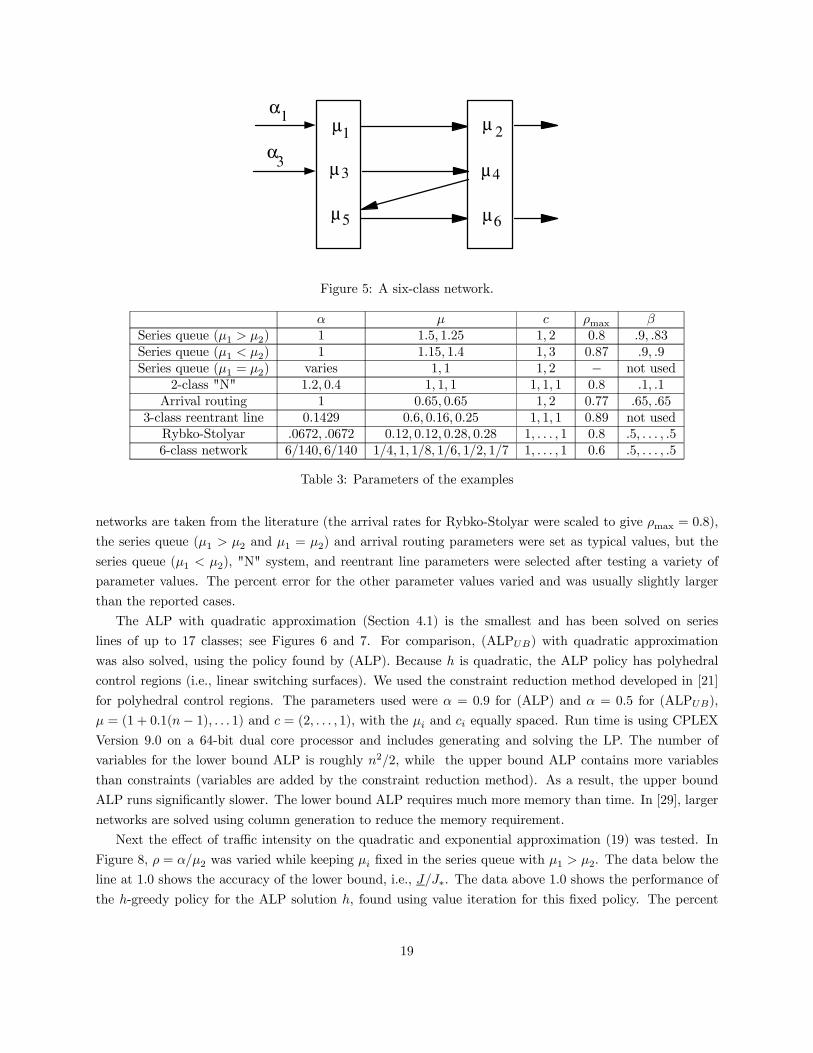
Figure 5: A six-class network.

α µ c ρmax βSeries queue (µ1 > µ2) 1 1.5, 1.25 1, 2 0.8 .9, .83Series queue (µ1 < µ2) 1 1.15, 1.4 1, 3 0.87 .9, .9Series queue (µ1 = µ2) varies 1, 1 1, 2 − not used

2-class "N" 1.2, 0.4 1, 1, 1 1, 1, 1 0.8 .1, .1Arrival routing 1 0.65, 0.65 1, 2 0.77 .65, .65

3-class reentrant line 0.1429 0.6, 0.16, 0.25 1, 1, 1 0.89 not usedRybko-Stolyar .0672, .0672 0.12, 0.12, 0.28, 0.28 1, . . . , 1 0.8 .5, . . . , .56-class network 6/140, 6/140 1/4, 1, 1/8, 1/6, 1/2, 1/7 1, . . . , 1 0.6 .5, . . . , .5

Table 3: Parameters of the examples

networks are taken from the literature (the arrival rates for Rybko-Stolyar were scaled to give ρmax = 0.8),

the series queue (µ1 > µ2 and µ1 = µ2) and arrival routing parameters were set as typical values, but the

series queue (µ1 < µ2), "N" system, and reentrant line parameters were selected after testing a variety of

parameter values. The percent error for the other parameter values varied and was usually slightly larger

than the reported cases.

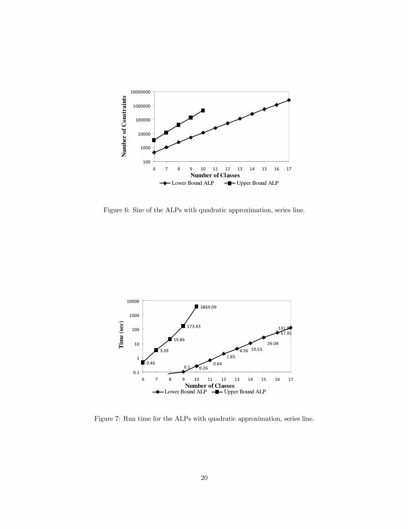
The ALP with quadratic approximation (Section 4.1) is the smallest and has been solved on series

lines of up to 17 classes; see Figures 6 and 7. For comparison, (ALPUB) with quadratic approximation

was also solved, using the policy found by (ALP). Because h is quadratic, the ALP policy has polyhedral

control regions (i.e., linear switching surfaces). We used the constraint reduction method developed in [21]

for polyhedral control regions. The parameters used were α = 0.9 for (ALP) and α = 0.5 for (ALPUB),

µ = (1 + 0.1(n− 1), . . . 1) and c = (2, . . . , 1), with the µi and ci equally spaced. Run time is using CPLEX

Version 9.0 on a 64-bit dual core processor and includes generating and solving the LP. The number of

variables for the lower bound ALP is roughly n2/2, while the upper bound ALP contains more variables

than constraints (variables are added by the constraint reduction method). As a result, the upper bound

ALP runs significantly slower. The lower bound ALP requires much more memory than time. In [29], larger

networks are solved using column generation to reduce the memory requirement.

Next the effect of traffic intensity on the quadratic and exponential approximation (19) was tested. In

Figure 8, ρ = α/µ2 was varied while keeping µi fixed in the series queue with µ1 > µ2. The data below the

line at 1.0 shows the accuracy of the lower bound, i.e., J/J∗. The data above 1.0 shows the performance of

the h-greedy policy for the ALP solution h, found using value iteration for this fixed policy. The percent

19

100

1000

10000

100000

1000000

10000000

6 7 8 9 10 11 12 13 14 15 16 17

Number of Classes

Nu

mb

er o

f C

on

stra

ints

Lower Bound ALP Upper Bound ALP

Figure 6: Size of the ALPs with quadratic approximation, series line.

57.95

131.85

0.46

3.39

19.86

173.43

3869.09

26.08

10.534.36

1.85

0.64

0.260.1

0.1

1

10

100

1000

10000

6 7 8 9 10 11 12 13 14 15 16 17

Number of Classes

Tim

e (

sec)

Lower Bound ALP Upper Bound ALP

Figure 7: Run time for the ALPs with quadratic approximation, series line.

20

0.5

0.6

0.7

0.8

0.9

1.0

1.1

1.2

1.3

0.0 0.1 0.2 0.3 0.4 0.5 0.6 0.7 0.8 0.9 1.0

Traffic intensity

J/J

*

Performance of ALP (Quad) ALP Bound (Quad)

Performance of ALP (EXP3) ALP Bound (EXP3)

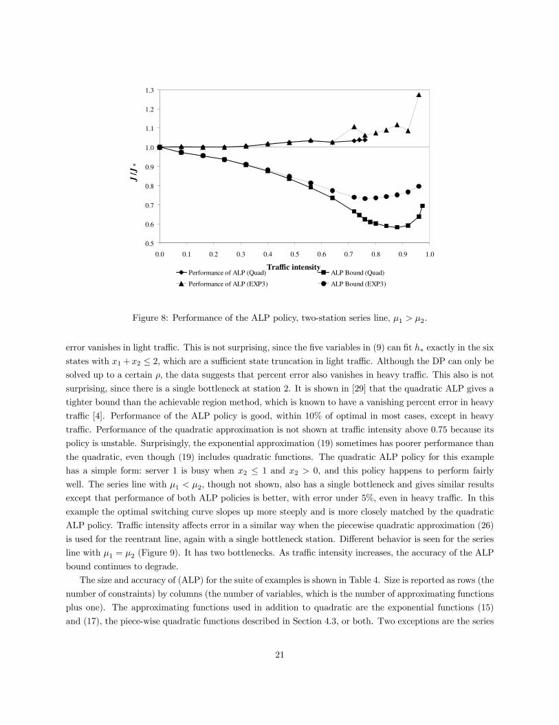
Figure 8: Performance of the ALP policy, two-station series line, µ1 > µ2.

error vanishes in light traffic. This is not surprising, since the five variables in (9) can fit h∗ exactly in the six

states with x1+x2 ≤ 2, which are a sufficient state truncation in light traffic. Although the DP can only be

solved up to a certain ρ, the data suggests that percent error also vanishes in heavy traffic. This also is not

surprising, since there is a single bottleneck at station 2. It is shown in [29] that the quadratic ALP gives a

tighter bound than the achievable region method, which is known to have a vanishing percent error in heavy

traffic [4]. Performance of the ALP policy is good, within 10% of optimal in most cases, except in heavy

traffic. Performance of the quadratic approximation is not shown at traffic intensity above 0.75 because its

policy is unstable. Surprisingly, the exponential approximation (19) sometimes has poorer performance than

the quadratic, even though (19) includes quadratic functions. The quadratic ALP policy for this example

has a simple form: server 1 is busy when x2 ≤ 1 and x2 > 0, and this policy happens to perform fairly

well. The series line with µ1 < µ2, though not shown, also has a single bottleneck and gives similar results

except that performance of both ALP policies is better, with error under 5%, even in heavy traffic. In this

example the optimal switching curve slopes up more steeply and is more closely matched by the quadratic

ALP policy. Traffic intensity affects error in a similar way when the piecewise quadratic approximation (26)

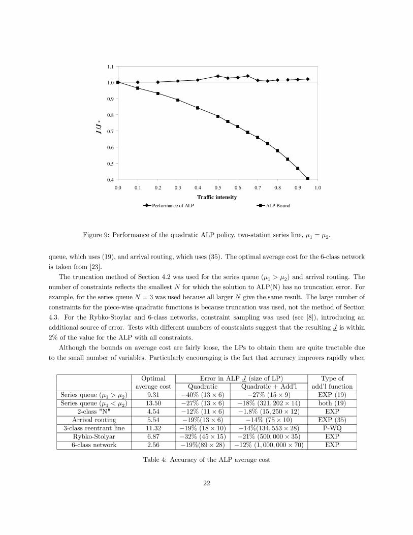
is used for the reentrant line, again with a single bottleneck station. Different behavior is seen for the series

line with µ1 = µ2 (Figure 9). It has two bottlenecks. As traffic intensity increases, the accuracy of the ALP

bound continues to degrade.

The size and accuracy of (ALP) for the suite of examples is shown in Table 4. Size is reported as rows (the

number of constraints) by columns (the number of variables, which is the number of approximating functions

plus one). The approximating functions used in addition to quadratic are the exponential functions (15)

and (17), the piece-wise quadratic functions described in Section 4.3, or both. Two exceptions are the series

21

0.4

0.5

0.6

0.7

0.8

0.9

1.0

1.1

0.0 0.1 0.2 0.3 0.4 0.5 0.6 0.7 0.8 0.9 1.0

Traffic intensity

J/J

*

Performance of ALP ALP Bound

Figure 9: Performance of the quadratic ALP policy, two-station series line, µ1 = µ2.

queue, which uses (19), and arrival routing, which uses (35). The optimal average cost for the 6-class network

is taken from [23].

The truncation method of Section 4.2 was used for the series queue (µ1 > µ2) and arrival routing. The

number of constraints reflects the smallest N for which the solution to ALP(N) has no truncation error. For

example, for the series queue N = 3 was used because all larger N give the same result. The large number of

constraints for the piece-wise quadratic functions is because truncation was used, not the method of Section

4.3. For the Rybko-Stoylar and 6-class networks, constraint sampling was used (see [8]), introducing an

additional source of error. Tests with different numbers of constraints suggest that the resulting J is within

2% of the value for the ALP with all constraints.

Although the bounds on average cost are fairly loose, the LPs to obtain them are quite tractable due

to the small number of variables. Particularly encouraging is the fact that accuracy improves rapidly when

Optimal Error in ALP J (size of LP) Type ofaverage cost Quadratic Quadratic + Add’l add’l function

Series queue (µ1 > µ2) 9.31 −40% (13× 6) −27% (15× 9) EXP (19)Series queue (µ1 < µ2) 13.50 −27% (13× 6) −18% (321, 202× 14) both (19)

2-class "N" 4.54 −12% (11× 6) −1.8% (15, 250× 12) EXPArrival routing 5.54 −19%(13× 6) −14% (75× 10) EXP (35)

3-class reentrant line 11.32 −19% (18× 10) −14%(134, 553× 28) P-WQRybko-Stolyar 6.87 −32% (45× 15) −21% (500, 000× 35) EXP6-class network 2.56 −19%(89× 28) −12% (1, 000, 000× 70) EXP

Table 4: Accuracy of the ALP average cost

22

more functions are added. Adding three exponential functions to the quadratic ALP for the series queue

with µ1 > µ2 cut the error from 40% to 27%. Adding three more exponential functions (15) and (17) reduced

the error to 18%. For the series queue with µ1 > µ2, these errors are 27%, 18%, and 12%. The piece-wise

quadratic functions were also fairly effective when added to the quadratic, reducing error from 19% to 14%

for the reentrant line. For the series queue with µ1 < µ2, the piece-wise quadratic approximation (not shown)

added 5 functions and reduced error from 27% to 21%. Based on Figure 8, these bounds should be tighter

in light traffic or single-bottleneck heavy traffic.

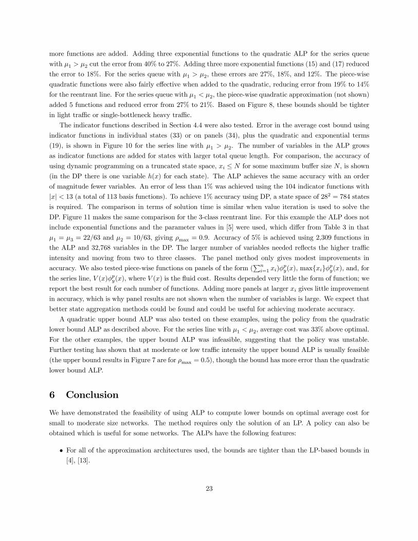
The indicator functions described in Section 4.4 were also tested. Error in the average cost bound using

indicator functions in individual states (33) or on panels (34), plus the quadratic and exponential terms

(19), is shown in Figure 10 for the series line with µ1 > µ2. The number of variables in the ALP grows

as indicator functions are added for states with larger total queue length. For comparison, the accuracy of

using dynamic programming on a truncated state space, xi ≤ N for some maximum buffer size N , is shown

(in the DP there is one variable h(x) for each state). The ALP achieves the same accuracy with an order

of magnitude fewer variables. An error of less than 1% was achieved using the 104 indicator functions with

|x| < 13 (a total of 113 basis functions). To achieve 1% accuracy using DP, a state space of 282 = 784 states

is required. The comparison in terms of solution time is similar when value iteration is used to solve the

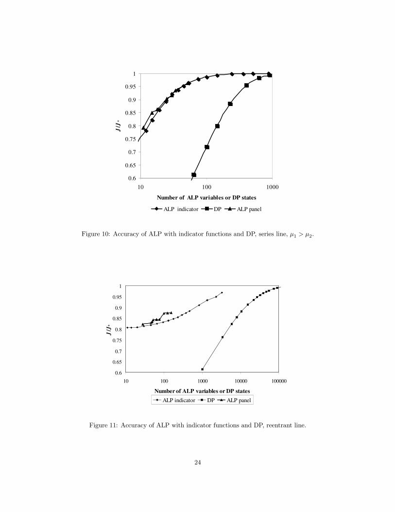
DP. Figure 11 makes the same comparison for the 3-class reentrant line. For this example the ALP does not

include exponential functions and the parameter values in [5] were used, which differ from Table 3 in that

µ1 = µ3 = 22/63 and µ2 = 10/63, giving ρmax = 0.9. Accuracy of 5% is achieved using 2,309 functions in

the ALP and 32,768 variables in the DP. The larger number of variables needed reflects the higher traffic

intensity and moving from two to three classes. The panel method only gives modest improvements in

accuracy. We also tested piece-wise functions on panels of the form (∑ni=1 xi)φ

py(x), max{xi}φ

py(x), and, for

the series line, V (x)φpy(x), where V (x) is the fluid cost. Results depended very little the form of function; we

report the best result for each number of functions. Adding more panels at larger xi gives little improvement

in accuracy, which is why panel results are not shown when the number of variables is large. We expect that

better state aggregation methods could be found and could be useful for achieving moderate accuracy.

A quadratic upper bound ALP was also tested on these examples, using the policy from the quadratic

lower bound ALP as described above. For the series line with µ1 < µ2, average cost was 33% above optimal.

For the other examples, the upper bound ALP was infeasible, suggesting that the policy was unstable.

Further testing has shown that at moderate or low traffic intensity the upper bound ALP is usually feasible

(the upper bound results in Figure 7 are for ρmax = 0.5), though the bound has more error than the quadratic

lower bound ALP.

6 Conclusion

We have demonstrated the feasibility of using ALP to compute lower bounds on optimal average cost for

small to moderate size networks. The method requires only the solution of an LP. A policy can also be

obtained which is useful for some networks. The ALPs have the following features:

• For all of the approximation architectures used, the bounds are tighter than the LP-based bounds in

[4], [13].

23

0.6

0.65

0.7

0.75

0.8

0.85

0.9

0.95

1

10 100 1000

Number of ALP variables or DP states

J/J

*

ALP indicator DP ALP panel

Figure 10: Accuracy of ALP with indicator functions and DP, series line, µ1 > µ2.

0.6

0.65

0.7

0.75

0.8

0.85

0.9

0.95

1

10 100 1000 10000 100000

Number of ALP variables or DP states

J/J

*

ALP indicator DP ALP panel

Figure 11: Accuracy of ALP with indicator functions and DP, reentrant line.

24

• The simplest, quadratic ALP has moderate accuracy and is fairly tractable. After constraint reduction,

the number of constraints in the LP grows linearly the number of control actions and the number of

buffers. Typically the number of actions is exponential in the number of buffers, but with a small base,

and the resulting LP can be solved for much larger networks than can be solved exactly by DP.

• Accuracy can be improved significantly by adding a set of roughly n2 exponential approximating

functions (where n is the number of buffers). New constraint reduction techniques were developed that

make ALPs with some of these exponential terms more tractable.

• Accuracy can also be improved by adding piece-wise quadratic approximating functions based on the

associated fluid model. The number of approximating functions depends on the complexity of the fluid

policy. General constraint reduction techniques were developed to help make these ALPs solvable.

• A sequence of ALPs with additional approximating functions that are indicators for individual states

or sets of states up to a maximum buffer size can be used to obtain more accurate bounds. On small

examples, the bounds require much less computation than using DP value iteration on a truncated

state space; however, this advantage diminishes when more accuracy is desired. This set of functions

is exponential in the number of buffers; the aggregation method reduces the base of the exponential

growth, making the method practical for somewhat larger networks.

In addition, two upper bounds on optimal average cost were proposed. The first, which involves solving a

second LP, gives fairly loose bounds, suggesting that simulation might be a better approach.

Several questions about the ALP approach remain open:

• More work is needed to determine larger sets of approximating functions that give tighter bounds. The

quadratic, exponential, and piece-wise quadratic functions consistently give moderate accuracy, but

accuracy improves more slowly as the indicator functions in Section 4.4 are added. We have begun

developing a larger set of rational functions that shows some promise.

• The piece-wise quadratic functions do not scale well to larger networks because computing the regions

Sk requires knowing the optimal policy for the fluid model. For larger networks, using the two-station

fluid relaxation in [17] might be a tractable alternative, as discussed in Section 4.3.

• The constraint reduction method for piece-wise quadratic functions in Section 4.3 has not been tested.

It would be interesting to test the speed and accuracy of ALP(N) compared to (ALPD).

• Performance of the policies recovered from the ALP remains a major open question. Numerical tests

show that the policies can have poor performance or be unstable. However, using different approxi-

mation architectures or combining the ALP policies with heuristics such as safety stocks might lead to

improved policies. It would be of interest to obtain bounds on their performance.

Appendix A Equivalence of LP form of the optimality equation

This appendix shows the equivalence of (1) to (LP) and (6). The argument is similar to, e.g., [20]. Using the

constraints for the optimal policy and letting xk denote the state after k transitions (including self-transitions

25

of the uniformized chain),

J ≤ c′xk +Eu∗ [h(xk+1)|xk]− h(xk).

After summing and telescoping, taking expectations yields

J ≤1

N

N−1∑

k=0

Ex,u∗c′xk +

1

NEx,u∗h(xN) +

1

Nh(x0).

We need to show that

limN→∞

1

NEx,u∗h(xN) = 0 (36)

so that taking the limit as N →∞ leaves J ≤ J∗ for any feasible h.. Then, since (J∗, h∗) are feasible, they

are optimal for (LP) and (6).

To show (36), use the fact that, for all policies u with finite J(x, u),

limN→∞

1

NEx,u |xN |

2 = 0 (37)

[12, Theorem 1]. Although they assume nonidling policies, (37) also holds for weakly nonidling policies where

u(t) = 0 if x(t) = 0, which includes u∗. Their result also assumes x is in the recurrent class, but for the

optimal policy this extends easily to all states. Combining (37) and (6) gives (36).

Appendix B ALP Constraints for the Series Queue

For the series queue of Section 4.2 and the differential cost approximation (19) this appendix gives the ALP

constraints in terms of z, where x = z + u. The terms in (18) are

h(x+ e1)− h(x) = q11x1 + q12x2 +1

2q11 + p1 + r2β

x2

h(x− e1 + e2)− h(x) = (−q11 + q12)x1 + (q22 − q12)x2 +1

2q11 +

1

2q22 − q12

− p1 + p2 − r1(1− β)βx2 − r2[(1− β)x1 + β]βx2 − r3[(1− β)x2 − β]βx2

h(x− e2)− h(x) = −q12x1 − q22x2 +1

2q22 − p2 + r1(

µ1µ2− 1)βx2

+ r2x1(µ1µ2− 1)βx2 + r3

[(µ1µ2− 1)x2 −

µ1µ2

]βx2 .

Using these, (18) can be written as (20), which we restate here

J ≤ du + cuT z + (ζu + ξuT z)βz2+u2 .

26

For the control u = (1, 1), ξ(1,1) = 0 and

c(1,1)1 = c1 − (µ1 − α)q11 + (µ1 − µ2)q12

c(1,1)2 = c2 − (µ1 − α)q12 + (µ1 − µ2)q22

d(1,1) = c(1,1)1 + c

(1,1)2 +

1

2(α+ µ1)q11 − µ1q12 +

1

2(µ1 + µ2)q22 − (µ1 − α)p1 + (µ1 − µ2)p2

ζ(1,1) = −r2(µ2 − α)− r3(µ1 − µ2).

For u = (0, 1),

c(0,1)1 = c1 + αq11 − µ2q12

c(0,1)2 = c2 + αq12 − µ2q22

d(0,1) = c(0,1)2 +

1

2αq11 +

1

2µ2q22 + αp1 − µ2p2

ξ(0,1)1 = r2(µ1 − µ2)

ξ(0,1)2 = r3(µ1 − µ2)

ζ(0,1) = ξ(0,1)2 + r1(µ1 − µ2) + r2α− r3µ1.

For u = (1, 0), we must have z2 = 0 and ξ(1,0)1 = 0, ζ(1,0) = 0,

c(1,0)1 = c1 − (µ1 − α)q11 + µ1q12 − r2(µ1 − µ2)

d(1,0) = c(1,0)1 +

1

2(α+ µ1)q11 − µ1q12 +

1

2µ1q22 − (µ1 − α)p1 + µ1p2

−r1(µ1 − µ2)− r2(µ2 − α) + r3µ2.

Finally, for u = x = (0, 0), ζ(0,0) = 0 and

d(0,0) =1

2αq11 + αp1 + αr2.

Acknowledgements

Much of the numerical work in this paper was done by Jonathan Senning and by my students Lauren

Berger, Taylor Carr, Lauren Carter, Jane Eisenhauer, Adam Elnagger, Jeff Fraser, Michael Frechette, Melissa

LeClair, Josh Nasman, Chris Pfohl, and Nathan Walker; Anna Moore and Daniel Stahl also assisted. I would

also like to thank Sean Meyn for his many suggestions. This work was supported in part by National Science

Foundation grant 0620787.

References

[1] D. Adelman. A price-directed approach to stochastic inventory/routing. Operations Research, 52(4):499—

514, 2004.

27

[2] F. Avram, D. Bertsimas, and M. Ricard. Fluid models of sequencing problems in open queueing

networks: An optimal control approach. In F.P. Kelly and R.J. Williams, editors, Stochastic Networks,

Vol. 71 of the IMA Volumes in Mathematics and its Applications, pages 199—234. Springer-Verlag, New

York, 1995.

[3] D. Bertsimas, D. Gamarnik, and J.N. Tsitsiklis. Performance of multiclass Markovian queueing networks

via piecewise linear lyapunov functions. Ann. Appl. Probab., 11:1384—1428, 2001.

[4] D. Bertsimas, I.Ch. Paschaladis, and J.N. Tsitsiklis. Optimization of multiclass queueing networks:

Polyhedral and nonlinear characterizations of achievable performance. Ann. Appl. Probab., 4:43—75,

1994.

[5] R-R. Chen and S.P. Meyn. Value iteration and optimization of multiclass queueing networks. Queueing

Systems Theory and Appl., 32(1-3):65—97, 1999.

[6] D.P. de Farias and B. Van Roy. Approximate linear programming for average-cost dynamic program-

ming. In Advances in Neural Information Processing Systems 15. MIT Press, 2003.

[7] D.P. de Farias and B. Van Roy. The linear programming approach to approximate dynamic program-

ming. Oper. Res., 51(6):850—865, 2003.

[8] D.P. de Farias and B. Van Roy. On constraint sampling for the linear programming approach to

approximate dynamic programming. Math. Oper. Res., 29(3):462—478, 2004.

[9] D.P. de Farias and B. Van Roy. A linear program for Bellman error minimization with performance

guarantees. In Advances in Neural Information Processing Systems 17. MIT Press, 2005.

[10] B. Hajek. Optimal control of two interacting service stations. IEEE Trans. Automat. Control, AC-

29:491—499, 1984.

[11] J.M Harrison. Heavy traffic analysis of a system with parallel servers: Asymptotic optimality of discrete-

review policies. Ann. Appl. Probab., 8(3):822—848, 1998.

[12] P.R. Kumar and S.P. Meyn. Duality and linear programs for stability and performance analysis of

queueing networks and scheduling policies. IEEE Trans. Automat. Control, 41(1):4—17, 1996.

[13] S. Kumar and P. R. Kumar. Performance bounds for queueing networks and scheduling policies. IEEE

Trans. Automat. Control, 39:1600—1611, 1994.

[14] S.P. Meyn. The policy iteration algorithm for Markov decision processes with general state space. IEEE

Trans. Automat. Control, AC-42:191—197, 1997.

[15] S.P. Meyn. Sequencing and routing in multiclass queueing networks. Part I: Feedback regulation. SIAM

J. Control Optim., 40:741—776, 2001.

[16] S.P. Meyn. Stability, performance evaluation and optimization. In E. Feinberg and A. Shwartz, editors,

Handbook of Markov Decision Processes: Methods and Applications. Kluwer, 2001.

28

[17] S.P. Meyn. Sequencing and routing in multiclass queueing networks. Part II: Workload relaxations.

SIAM J. Control Optim., 42(1):178—217, 2003.

[18] S.P. Meyn. Dynamic safety-stocks for asymptotic optimality in stochastic networks. Dept. of Electrical

and Computer Eng., University of Illinois at Urbana-Champaign, 2004.

[19] C.C. Moallemi, S. Kumar, and B. Van Roy. Approximate and data-driven dynamic programming for

queueing networks. Working paper, Graduate School of Business, Columbia University, 2006.

[20] J.R. Morrison and P.R. Kumar. New linear program performance bounds for queueing networks. J.

Optim. Theory Appl., 100(3):575—597, 1999.

[21] J.R. Morrison and P.R. Kumar. Computational performance bounds for Markov chains with ap-

plications. IEEE Trans. Autom. Control, 53:1306—1311, 2008. Full-length version available at

http://black.csl.uiuc.edu/∼prkumar.

[22] C.H. Papadimitriou and J.N. Tsitsiklis. The complexity of optimal queuing network control. Math.

Oper. Res., 24:293—305, 1999.

[23] I.C. Paschaladis, C. Su, and M.C. Caramanis. Target-pursuing scheduling and routing policies for

multiclass queueing networks. IEEE Trans. Automat. Control, 49(10):1709—1722, July 2004.

[24] M. C. Russell, J. Fraser, S. Rizzo, and M. H. Veatch. Comparing LP bounds for queueing networks. To

appear, IEEE Trans. Autom. Control, 2009.

[25] D. Schuurmans and R. Patrascu. Direct value-approximation for factored MDPs. In Advances in Neural

Information Processing Systems 14, pages 1579—1586. MIT Press, 2001.

[26] P. Schweitzer and A. Seidmann. Generalized polynomial approximations in Markovian decision

processes. J. of Mathematical Analysis and Applications, 110:568—582, 1985.

[27] L.I. Sennott. Stochastic Dynamic Programming and the Control of Queueing Systems. Wiley, New York,

1999.

[28] H. Topaloglu and S. Kunnumkal. Approximate dynamic programming methods for an inventory allo-

cation problem under uncertainty. Naval Research Logistics, 53:822—841, 2006.

[29] M. H. Veatch and N. Walker. Approximate linear programming for network control: Col-

umn generation and subproblems. Working paper, Gordon College, Dept. of Math. Available at

http://faculty.gordon.edu/ns/mc/mike-veatch, 2008.

[30] M.H. Veatch. Fluid analysis of arrival routing. IEEE Trans. Automat. Control, 46:1254—1257, 2001.

[31] M.H. Veatch. Using fluid solutions in dynamic scheduling. In S. B. Gershwin, Y. Dallery, C. T.

Papadopoulos, and J. M. Smith, editors, Analysis and Modeling of Manufacturing Systems, pages 399—

426, New York, 2002. Kluwer.

[32] G. Weiss. On optimal draining of fluid reentrant lines. In F.P. Kelly and R.J. Williams, editors,

Stochastic Networks, Vol. 71 of the IMA Volumes in Mathematics and its Applications, pages 93—105,

New York, 1995. Springer-Verlag.

29