Put-Call Parity

chris bemis

May 22, 2006

Recall that a replicating portfolio of a contin-

gent claim determines the claim’s price.

This was justified by the ”no arbitrage” prin-

ciple.

Using this idea, we obtain a relationship be-

tween a European call and a European put

option.

1

Consider the following portfolios:

Portfolio 1: A European call option, and cash

at time t equal to Ke−rT

Portfolio 2: A European put option, and one

share of the underlying, S

Here, K is the strike price for both the call

and the put, and T is the time to expiration

for both options.

2

At maturity, Portfolio 1 is worth

K + max(ST − K,0) = max(ST , K),

and Portfolio 2 is worth

ST + max(K − ST ,0) = max(K, ST ).

Since the options are European, the prices to-

day of these portfolios must be the same.

If the prices were different, there would be an

arbitrage opportunity (just like the gold exam-

ple).

3

We have now that

c0 + Ke−rT = p0 + S0 (1)

This relationship is put-call parity, and holds

for European options.

Notice that this relationship is not model dependent-

we only relied on the no arbitrage principle.

4

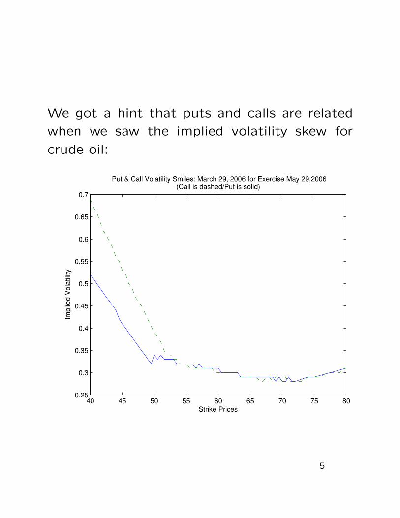
We got a hint that puts and calls are related

when we saw the implied volatility skew for

crude oil:

40 45 50 55 60 65 70 75 800.25

0.3

0.35

0.4

0.45

0.5

0.55

0.6

0.65

0.7

Put & Call Volatility Smiles: March 29, 2006 for Exercise May 29,2006(Call is dashed/Put is solid)

Strike Prices

Impl

ied

Vola

tility

5

Recall that the only unobservable quantity in

the Black-Scholes price of a European call or

put was the volatility.

Suppose that for a certain volatility, σ, we ob-

tain prices pB and cB for a put and call (resp.)

from the Black-Scholes model.

Since we assume the BS model is arbitrage

free, we must have

cB,0 + Ke−rT = pB,0 + S0.

Further, if the market is arbitrage free, we

must have a similar relationship for market prices,

pM and cM :

cM,0 + Ke−rT = pM,0 + S0.

This yields

cB,0 − cM,0 = pB,0 − pM,0

6

Now suppose the implied volatility for a call is

19%. When we use this volatilty,

cB,0 − cM,0 = 0

Hence, from the relation above, the market

price of the put must yield the same implied

volatility.

So we have:

The implied volatility for a European call op-

tion is the same as the implied volatility for a

European put option.

7

What about American options?

Recall an American option is the same as a Eu-

ropean option except that exercise may occur

any time up to and including the expiration of

the option.

We can’t use the same reasoning to obtain a

put-call parity result here since actions may be

taken at any time before maturity.

We will denote an American calls and puts by

C and P respectively.

8

Clearly, we must have

C ≥ c

since an American option has all of the prop-

erties of a European option and more.

Now consider the two portfolios:

Portfolio A’ : one European call option and

cash equal to Ke−rT

Portfolio B’ : one share

Assuming the cash is invested at the risk free

interest rate, Portfolio A’ is worth max(ST , K)

at maturity.

Portfolio B’ is worth ST .

So, we must have c ≥ S0 − Ke−rT

9

Because options have no downside risk, we

have

c ≥ max(S0 − Ke−rT ,0)

And hence

C ≥ max(S0 − Ke−rT ,0) > S0 − K.

But this implies that the option will never be

exercised early.

So an American call option (on a nondividend

paying stock) is the same as a European call

option.

10

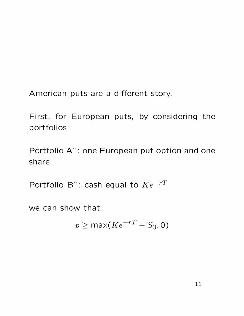
American puts are a different story.

First, for European puts, by considering the

portfolios

Portfolio A”: one European put option and one

share

Portfolio B”: cash equal to Ke−rT

we can show that

p ≥ max(Ke−rT − S0,0)

11

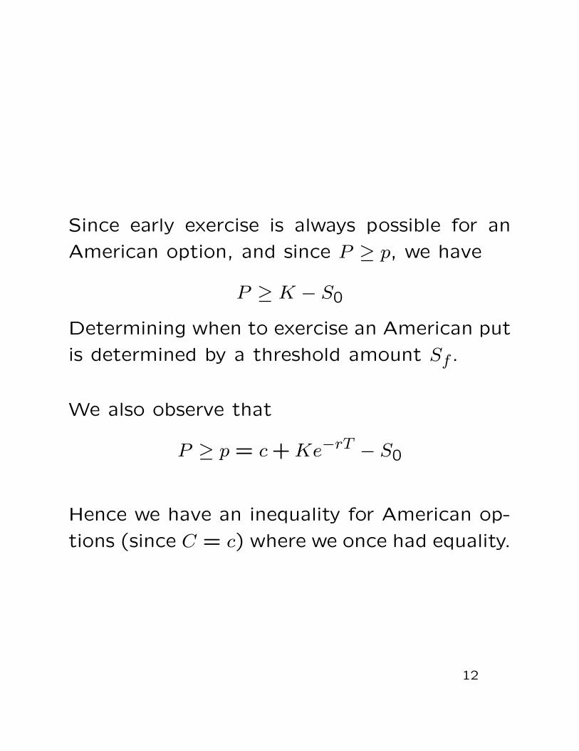
Since early exercise is always possible for an

American option, and since P ≥ p, we have

P ≥ K − S0

Determining when to exercise an American put

is determined by a threshold amount Sf .

We also observe that

P ≥ p = c + Ke−rT − S0

Hence we have an inequality for American op-

tions (since C = c) where we once had equality.

12

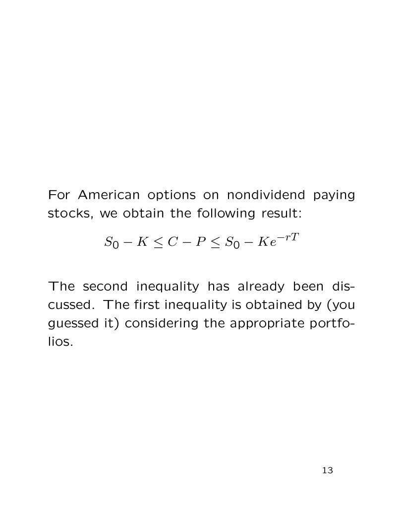
For American options on nondividend paying

stocks, we obtain the following result:

S0 − K ≤ C − P ≤ S0 − Ke−rT

The second inequality has already been dis-

cussed. The first inequality is obtained by (you

guessed it) considering the appropriate portfo-

lios.

13

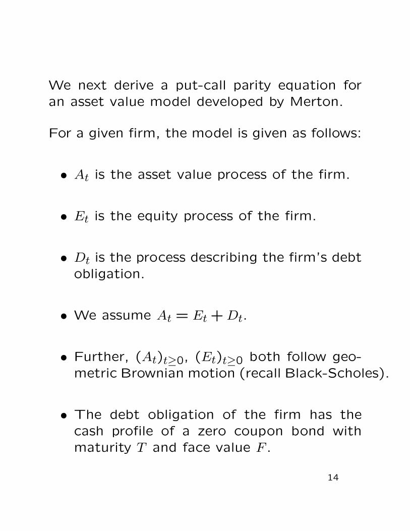
We next derive a put-call parity equation for

an asset value model developed by Merton.

For a given firm, the model is given as follows:

• At is the asset value process of the firm.

• Et is the equity process of the firm.

• Dt is the process describing the firm’s debt

obligation.

• We assume At = Et + Dt.

• Further, (At)t≥0, (Et)t≥0 both follow geo-

metric Brownian motion (recall Black-Scholes).

• The debt obligation of the firm has the

cash profile of a zero coupon bond with

maturity T and face value F .

14

Because of the last bullet, the cash profile of

debt is simple:

• At time t = 0, debt holders (think banks)

pay to the firm an amount of capital equal

to D0

• At time t = T , these debt holders receive

an amount of capital equal to F .

The debt holders have some risk if the value

of the firm’s assets at time T can be below F .

That is, riskiness is involved if

P[AT < F ] > 0,

in which case we must have D0 < Fe−rT .

15

If AT < F , the firm will default on its debt, and

the debt holders will only receive a fraction of

F .

The debt holders may want to neutralize this

risk. One way to do this is to go long a put

option on the asset, A, with strike price F , and

time to maturity T .

It is easy to show that the debt holder is now

gauranteed to receive F at time T

The debt holders are now completely hedged.

The hedged portfolio for the debt holders con-

sists of a loan and a put option, and has value

at time t = 0 of

D0 + PA,

where PA is the put as described above.

16

Because the hedged portfolio is worth F at

time T surely, we must have

D0 + PA = Fe−rT ,

or

D0 = Fe−rT − PA. (2)

We may also view equity in this option theo-

retic light. Suppose that at time T , the share-

holders decide to liquidate the firm. That is,

pay off all debts and receive capital for all as-

sets. We will consider two cases.

17

• If AT > F , the shareholders receive an amount

of capital equal to AT − F .

• If AT < F , the value of the assets of the

firm is not great enough to pay off the

debt. Hence there is nothing left over for

shareholders and their payoff is 0.

This sounds like a call option. In fact, we see

the payoff for equity holders is max(AT −F,0).

By no arbitrage arguments, we must have

E0 = CA, (3)

where CA is a call option with underlying A,

strike price F , and time to maturity T .

18

Putting this all together, we have

A0 = E0 + D0 = CA + Fe−rT − PA,

rearranging,

A0 + PA = CA + Fe−rT ,

which is just put-call parity with underlying A.

Before concluding, we note two results of the

model.

• Since E0 = CA, equity holders prefer assets

with more volatility.

• Because D0 = Fe−rT − PA, debt holders

(think banks) are naturally short a put and

therefore they prefer lower volatility.

19

There are some issues with the above model.

The biggest is that the asset value process is

not observable.

We may approximate the firm’s equity (shares

of stock) and its debt.

Abstracting the asset value process requires a

little more work, and can be tackled another

day.

20