Embed Size (px)
Citation preview

AEDC-TR-91-24
AD-A244 075
Asymptotic Theory of TransonicWind Tunnel Wall Interference
N. D. Malmuth, C. C. Wu, H. Jafroudi,R. Mclachlan, J. D. Cole, and R. Sahu
Rockwell International Science Center1049 Camino Dos Rios
Thousand Oaks, CA 91360
December 1991
Final Report for Period March 30, 1984 through July 30, 1990
DTICMaJAN 0 6 1992
0Approved for public release; distribution is unlimited.
92-00201
ARNOLD ENGINEERING DEVELOPMENT CENTERARNOLD AIR FORCE BASE, TENNESSEE
AIR FORCE SYSTEMS COMMANDUNITED STATES AIR FORCE

NOTICES
When U. S. Government drawings, specifications, or other data are used for any purposeother than a definitely related Government procurement operation, the Government therebyincurs no responsibility nor any obligation whatsoever, and the fact that the Governmentmay have formulated, furnished, or in any way supplied the said drawings, specifications,or other data, is not to be regarded by implication or otherwise, or in any manner licensingthe holder or any other person or corporation, or conveying any rights or permission tomanufacture, use, or sell any patented invention that may in any way be related thereto.
Qualified users may obtain copies of this report from the Defense Technical InformationCenter.
References to named commercial products in this report are not to be considered in anysense as an endorsement of the product by the United States Air Force or the Government.
This report has been reviewed by the Office of Public Affairs (PA) and is releasable tothe National Technical Information Service (NTIS). At NTIS, it will be available to thegeneral public, including foreign nations.
APPROVAL STATEMENT
This report has been reviewed and approved.
MARK S. BRISKI, Capt, USAFDirectorate of TechnologyDeputy for Operations
FOR THE COMMANDER
KEITH L. KUSHMANDirector of TechnologyDeputy for Operations

RACYU E PORTReebe 1991MFinAI-Form Approved
4. TITLE AODU MBTATLO P. UND IGMB No. 0704-0188
Public reporting burden for this collecion of information is e Wtimated to average I hour per response r including the time fo reviewing instructions, searching existing data ources,gatheringaandreviewigthecoectinofinfomatin Send comments regarding this burden estimate or any other aIt n i at of thiscollection of information. including suggestions fo, reducing this burden, to Washington Headquarters Services. Directorate for Information Operations and Reports. 12 15 Jefferson
Davis Hig hway. Svite 1 204, Arlington, VA 22202*4302, and to the Office of M anag ement and Bud jet, Paperwork Reduction Protect (0704-0158), WashingIton, DC 20503
1. AGENCY USE ONLY (Leave blank) 2. REPORT DATE 3. REPORT TYPE AND DATES COVEREDI December 1991 Final - Mar. 30, 1984 - July 30, 1990
4. TITLEANDSUBTITLE 5R FUNDING NUMBERS
Asymptotic Theory of Transonic Wind Tunnel Wall InterferenceStudy PE 65807F
6. AUTHOR(S)Malmuth, N. D., Wu, C. C., Jafroudi, H., Mclachlan, R., Cole, J. D.,and Sahu, R., Rockwell International Science Center
7 PERFORMING ORGANIZATION NAME (S) AND ADDRESS(ES) 8. PERFORMING ORGANIZATIONREPORT NUMBER
Rockwell International Science Center AEDC-TR-91-241049 Camino Dos RiosThousand Oaks, CA 91360
9. SPONSORING/MONITORING AGENCY NAMES(S) AND ADDRESS(ES) 10. SPONSORING/MONITORINGAGENCY REPORT NUMBER
Arnold Engineering Development Center/DOTAir Force Systems CommandArnold Air Force Base, TN 37389-5000
11 SUPPLEMENTARY NOTES
Available in Defense Technical Information Center (DTIC).
12a DISTRIBUTION/AVAILABILITY STATEMENT 12b. DISTRIBUTION CODE
Approved for public release; distribution is unlimited.
13 ABSTRACT (Maximum 200 words)
Two limiting cases are considered related to transonic wall interference. For the firstcorresponding to slender airplanes, an area rule for interference holds in which theinterference of the complete airplane can be obtained from that of its equivalent body ofrevolution. For large wall height, the slender case exhibits an asymptotic triple deckstructure consisting of a cross flow-dominated zone near the model, a weakly perturbedfree-field mid field which has a linear multipole far field for solid and free-jet wallconditions. Nonclassical, experimentally determined pressure conditions prescribed on acylindrical interface lead to a "tube vortex" far field. For a high aspect ratio second case, theinterference is driven by the imaging effect of the interface on the projection of the trailingvortex system in the Trefftz plane. This gives a downwash correction to a near-fieldnonlinear lifting line flow. Slightly subsonic free-stream conditions give a spike-likeinterference flow field due to the shock movement for both limiting cases. Computer codeswritten to treat these cases, as well as the underlying numerical methods, are described.Approaches integrating the asymptotics with measurement to augment Wall InterferenceAssessment/Correction (WIAC) procedures are outlined.
14 SUBJECT TERMS 15 NUMBEROFPAGEStransonic flow tunnels perturbation theory fluid dynamics 229asymptotic series numerical anaiysis 16 PRICE CODEtransonic flow aerodynamics
17 SECURITY CLASSIFICATION 18 SECURITY CLASSIFICATION 19 SECURITY CLASSIFICATION 20 LIMITATION OF ABSTRACTOF REPORT OF THIS PAGE OF ABSTRACTUNCLASSIFIED UNCLASSIFIED UNCLASSIFIED Same as Report
COMP'JTfR CNFRATED Standard Form 298 (Rev. 2-89)Prv' lbed by ANSI Sid 139 1929R-102

AEDC-TR-91-24
PREFACE
This report constitutes the final report of the Air Force contract F40600-84-COOIO,
Asymptotic Theory of Transonic Wind Tunnel Wall Interference Study. This effort was
conducted under the sponsorship of Arnold Engineering Development Center (AEDC), AirForce Systts Command (AFSC), Arnold Air Force Base, Tennessee 37389. Dr. Keith
Kushman and Captain Mark Briski, USAF, were the AEDC technical representatives for
the contract. The manuscript was submitted for publication on August 1, 1990. Editorial
comments were provided by J. Erickson and W. Sickles of Calspan. Reproducibles used inthe publication of this report were supplied by the authors. AEDC has neither edited nor
altered this manuscript.
2 .- i , r ,3
i, N\ K,: t -
- y
D , t

AEDC-TR-91-24
TABLE OF CONTENTS
Page
P reface . . . . . . . . . . . . . . . . . . . . . . . . . . . . . . . . . . iTable of Contents .......... .............................. . .iList of Illustrations ............ ............................. vList of Tables ............. ................................ x1. Introduction ............ .............................. 12. Confined Slender Configurations ......... ...................... 5
2.1 Treatment of Pressure Specified Interface Boundary Conditions ... ...... 52.1.1 KG Theory ........... ........................... 62.1.2 Problem Q: ........... ........................... 72.1.3 Large H Theory . . . . . . . . . . . . . . . . . . . . . . . . . 72.1.4 Cential Layer ........... .......................... 72.1.5 Free Field Approximation ....... .................... 72.1.6 Variational Equations ........ ....................... 72.1.7 Wall Layer ........... ............................ 92.1.8 Behavior of po near Origin ........ ..................... 92.1.9 Asymptotic Representation of (2 - 16) as R t --* 0 .... ........... 112.1.10 Matching .......... ............................ .122.1.11 Discussion ......... ........................... .15
2.2 Generalization to Angular and Unsymmetrical Variations ........... .162.2.1 Discussion .......... ............................ .20
2.3 Shock Jump Conditions .......... ........................ 202.4 Shock Conservation Laws for Wall Correction Flow ... ............ .242.5 Regularization of the Problem for the Correction Potential 1 ......... .262.6 Basic Code Modules ......... ......................... 272.7 Upstream and Downstream Far Fields ....... ................. 272.8 Difference Equations for the Wall Interference Correction Potential ....... 332.9 Finite Height Application of Zeroth Order Code ... ............. .. 352.10 Improved Accuracy Procedures for Numerical Treatment of Body Boundary
Conditions ............ ............................ 402.10.1 Results .......... ............................. 44
2.11 Shock Fitting Scheme for Wall Interference Correction Potential ........ 512.12 Determination of Second Term of Central Layer Large Height Expansion . . 552.13 Structural Aspects of Slender Body Code ..... ................ 562.14 Incompressible Validation of Interference Module RELAXV1 ......... .602.15 Transonic Application of Free Field and 0 th Order Code ........... .602.16 Fuither Remarks on Difference Schemes near Shock Notch .......... .68
2.16.1 Bidiagonal Approach ....... ....................... .682.16.2 Tridiagonal Methodology ........ ..................... 75
2.17 Definitions of Interference-Free Conditions in Wind Tunnels fromAsymptotic Slender Body Code ...... ................... .76
2.18 Determination of Interference-Free Flows ..... ................ 77
iii

AEDC-TR-91-.24
Page
2.19 Numerical Implementation. .. ....... ........ ..... 792.20 Results .. .. ...... ........ ........ ...... 82
3. Large Aspect Ratio Configurations. .... ........ ........ 933.1 Theory of Far Field Boundary Conditions. .. ...... ........ 93
3.1.1 Solid Wall and Free Jet Corrections .. .. ......... ..... 933.1.1.1 Discussion .. .... ......... ........ ... 933.1.1.2 Analysis .. .... ........ ........ ...... 94
3.1.2 Pressure Specified Boundary Conditions .. ... ........ .. 1043.2 Numerical Procedures and Outline of Code. ... ........ ... 109
3.2.1 Boundary Value Problem for 00 .. ........ ........ 1103.2.1.1 Analytic Formulation. ... ........ .......... 1103.2.1.2 Numerical Fom11ulatn. ..... .. .. ..... .. ..... .. .... 110
3.2.2 The Three-Dimensional and Wall Interference Correction 01 .. .. .. 1183.2.2.1 Analytic Formuletion. ... ........ .......... 1183.2.2.2 Numerical Formulation .. .. ....... ........ .. 1213.2.2.3 Program Operation and Flow Chart .. ... ........ .. 128
3.2.3 Convergence Acceleration. .. ...... .. .......... 1333.3 Results for Subcritical Interference Flows .. ..... .......... 1373.4 Supercritical Interference Flows .. ....... ........ ... 150
3.4.1 Refinements of Shock Fitting Procedures. .. .... ........ 1533.5 Computational Implementation of Pressure Specified Boundary
Conditions .. ..... ......... ........ .... 1603.6 Viscous Effects .. .. ....... ......... ........ 1653.7 Nonsimilar Section Wings and Lockheed Database. .. .......... 165
3.7.1 Swept Wing Comparison Database .. ...... ....... .. 1703.7.2 Code Generalization to Nonsimilar Section Wings. .. .... .... 1703.7.3 Results. .. ........ ......... .......... 1743.7.4 Discussion. .. ...... ........ ........ ... 174
3.8 Fuselage Effects .. ...... ........ ........ ... 1793.8.1 Discussion. .. .. ..... ........ ........ ... 185
4. Asymptotics Integrated with Measurement (AIM) Wall InterferenceMethods. .. ........ ......... .......... 186
4.1 Interference on Moderate and Low Aspect Ratio Configurations. .. ... 1864.2 High Aspect Ratio Configuration WIAC Method. .. ...... .... 192
4.2.1 Discussion. .. ...... ........ ........ ... 1965. Conclusions, Highlights and Summary of Findings .. ... .......... 1976. Recommendations. .. ..... ........ ........ .... 2037. References .. ..... ........ ........ ........ 206Nomenclature. .... ........ ........ ........ .. 210Appendix A - Models for Interference Flow Near Shocks. .. ......... 214Appendix B - Reexpansion. Singularity Details. .. .... ........ .. 216
iv

AEDC-TR-91-24
LIST OF ILLUSTRATIONS
Figure Page
1 Comparison of computational area rule with experiment .... ......... 32 Control surface in tunnel ......... ....................... 83 Matching of central and wall regions for axially symmetric
interface pressures ................................. .144 Spherical coordinates ........ ......................... .175 General case of matching of central region and wall layers ........... .. 196 Orientation of shock surfaces . . . . ..... ........... 21
7 Regions appropriate to shock conservation laws .... ............... 258 Flow chart for preprocessor and solver ..... ................. .289 Model confined by solid cylindrical w7.,alls and control volume ........... 32
10 Area distribution of blended wing fighter configuration .... .......... 3611 IsoMachs over blended wing configuration in free field, Mo, = .95 ..... .. 3712 Finite height solid wall interference effect at Moo = .95 on blended fighter
configuration equivalent body - Mach number distributionover body ..... ............. ............... 38
13 Finite height solid wall interference effect at Mo, = .95 on blended fighterconfiguration equivalent body - surface pressures .. ........... .. 39
14 Validation of RELAX1 code against Couch experiment, B- body, M = .99 . 4115 Nodes in vicinity of axis ........ ....................... .4216 Iterative convergence study of g ....... .................... .4617 Mesh convergence study of g (DASH2 legc,.d
is the dash-dot curve) .... ....................... 4718 Iterative convergence study of g'(x) ...... .................. .4819 Roundoff study of g'(x) ........ ........................ 4920 Roundoff study of g'(x) ........ ........................ 5021 Interference pressures on a confined parabolic arc body. H -. 1.1,
100 x 50 grid, 1200 iterations ........ .................... 5222 Schematic of shock fitting geometry for wall interference correction
potential ........... ............................. 5323 Comparison of exact and appre'-irmate integrands .... ............ .5724 Integrands used in evaluation of a0. . . . . . . . . . . . . . . . . . . .. . . . . . . 5825 Convergence study of ao integration ....... .................. 5926 Scheme for handling jumps in vertical velocities acioss shocks ........ .. 61
27a Sonic bubble over a parabolic arc body at Moo = 99, (A supersonicpoints, 0 subsonic points) ......... ...................... 62
27b Closeup of shock notch for configuration of Fig. 27a, (x signifies pointsfor which lM® - MAI > .01) ....... .................... .62
27c Typical overview of notch in relation to sonic line, Mc, = .99, NU = 0,ND = 2, JDEL = 0, NSPMAX = 66, NSPMIN = 59, JSMAX = 19. . .. 63
28 Logarithmic singularities associated with parabola of revolution ....... .64
VI

AEDC-TR-91-24
Figure Page
29 Comparison of analytical (approximate) and transonic variational codecomputation of interference pressures in subsonic flow ............ .65
30 Convergence study of incompressible free field solution, b = .178 ........ 6631 Grid used in solution ........ ......................... .6732 00, behavior near the body ........ ...................... 6733 Streamwise distribution, parabolic arc body, Moo = 0.99 ............ .6934 Formation of shock ........... .......................... 6935 isoMachs showing closeup of shock ....... ................... 7036 Perturbation velocity v0 over the parab :Iic body at Moo = 0.99 ......... 7037 Closeup of Fig. 36 v0 distribution near shock ...... .............. 7138 u0 distribution for M = 0.99 parabolic arc body .... ............ .7239 Closeup of Fig. 34 ito dist-ributir.. ..... ................... .7240 Three-dimensional relief of 00 field for Moo = 0.99 parabolic arc body . . 7341 Three-dimensional relief of 00. field for M = 0.99 parabolic arc body . 73
42a Schematic of ACD versus K 1 . . . . . . . . . . . . . . . . . . . .. . . . . . . . . 7842b Schematic of variation of interference-free KI with K 0 . . . . . . . . . 7 8
43 Interference drag versus interference similarity parameter ........... .. 8044 Shock jump geometry .......... ........................ 81
45a ERRMAX convergence history for 0 th order flow parabolic arc body,b = .1, A. = .99 ...... ......................... 83
45b CD convergence history for 0 th order flow, parabolic arc body,= .1, AL, = .99 ......... ......................... 83
46a Variational solver convergence history, parabolic arc body,MVI = .99, 6 = .1 ........ ......................... .84
46b Variational solver convergence history, parabolic arc body,Mo = .99, 6 = .1 ......... ......................... 84
47 Free field 0th order Cp for various Mach numbers, 6 = .1, parabolicarc body .......... ............................. .86
4S Normalized interference Cp, ACpH 3 /6 2 , parabolic arc body, forMw = .99, 6 = .1, (K = 1.99) ........ .................... 87
49 K dependence of reduced interference pressures - bidiagonal scheme forshock jumps .......... ............................ 88
50 Comparison of 0 th order and total CP unscaled H = 10+, parabolicbody, STINT25, 1oo = .99, b = .1, bidiagonal scheme,K = 1.99 .......... .. ............................. R9
51 Sensitivity of interference pressures to notch size parameters, parabolicarc body, 6 = .1, Mo = .99, (K = 1.99) ..... ................ 91
52 Normalized interference drag ACDH3 /62 as a function of transonicsimilarity parameter K = (1 - M2)/6 . . . . . . . . . . . . . . . . . . . . . . 92
53 Lifting line in rectangular cross section wind tunnel ..... ........... 9554 High aspect ratio wing within cylindrical pressure specified control
surface ............. .............................. 96
vi

AEDC-TR.91 24
Figure Page
55 Far field flow configuration showing lifting line and vortex sheet ....... .9756 Angular variables for Green's function associated with cylindrical
walls ........................................ 9857 Contour for inversion of the inner integral in Eq. (3 - 51) .......... ... 10858 Airfoil geometry .......... .......................... 11159 Computational grid .......... ........................ 11160 Flow chart for MAIN program computing €o .... ............. .. 11461 Flowchart of subroutine MKFOIL ........ .................. 11562 Angular relations for far field ....... .................... .. 11563 Flowchart for subroutine SOLVE ...... ................... .. 11664 Flowchart for subroutine SLOR ...... ................... .. 11765 Elliptic planform. .............................. 119
66 Front view of wing confined in circular wind tunnel ............. .. 12067 Arguments .Ised in Eq. (3 - 70) ......................... .. 12368 Orientation of shock notch ....... ..................... .. 12569 Linear extrapolation at shock ...... .................... ... 125
70a Wide shock notch ......................... 12770b One point shock notch ........ ....................... .. 12770c Three point shock notch ........ ...................... .. 127
71 Periodic extension of planfori ........................ 13172 Computational molecule used in SETUP ...... .............. 13173 Pre and post shock sides of shock notch ..... ................ .. 13174 Flowchart of postprocessing elements ..... ................. .. 13475 Flowchart of subroutine SLOR ....... .................... .. 13576 Effect of convergence acceleration on attainment of asymptotic value of
circulation " .......... .......................... .. 13877 Mean wing chordwise pressures, circular open jet test scction
wind tunnel, M,, =.63, a = 2', NACA 0012 airfoil, 100 x 60 grid,elliptic planform ........ ......................... .. 139
78 IsoMachs for zeroth order flow for wing of Fig. 77 ... ........... .. 14079 Perturbation (01) isoMachs for wing of Fig. 77 ...... ............ 141
80 Total (€0 + 1) isoMachs for wing of Fig. 77 ..... ............. 142
81 Variation of the chordwise pressure distribution along the span for wingof Fig. 77, M, = .63, a = 2 ........ ................... 144
82 Spanwise loading for wing of Fig. 77 ....... ................. 14583 Spanwise loading for nonelliptic wing. All other parameters identical to
those associated with Fig. 77 ...... ................... .. 14684 Pressure distributions over NACA 0012 airfoil, WMoo = .75, a = 2',
50 x 50 grid, Ay = .05, AJ = 1 ...... .................. .. 147
vii
AEDC-TR-91-24
Figure Page
85 Pressure distributions over NACA 0012 airfoil, Mo .75, a = 20,98 x 60 grid ........... ........................... 148
86 Variation of perturbation downwash with pressure in relation to shockhodograph, M,, = .75, a = 20, NACA 0012 airfoil ............. .. 149
87 IsoMachs for NACA 0012 airfoil, Moo = .8, a = 20, grid adapted toleading edge bluntness ........ ..................... 151
88 Chordwise pressures on elliptic planform wing inside open jet windtunnel, AR = 8.0, Moo = 0.7, a = 20, y = 1.05, NACA 0012 airfoil,100 x 60 grid ........ ... .......................... 152
89 Flow chart of OUTPUT module relevant to variational solver forinterference potential, repeated version of Fig. 74 for convenience . 154
9(, Circulation perturbation convergence, M,, = 0.75, a -= 20. elliptic
planform, NACA 0012 airfoil ..... ... ................... 15591 Free field isoMachs for Mo, = 0.75, a = 20, AR = 8, ellipti,
planform, NACA 0012 airfoil section ..... ................ ... 15692 Free field isoMachs for Moo = 0.75, a = 20, AR = 8, elliptic
planform, NACA 0012 airfoil section - close up . .... 15793 Free jet wind tunnel corrected isoMachs for Mo, = 0.75, a = 20,
AR = 8, t = 1.05, elliptic planform, NACA 0012 airfoil section . ... 15894 Chordwise pressures along span in free field, M,, = .75, a = 20,
elliptic planform, NACA 0012 airfoil section ... ............. .. 16195 Mean chordwise pressure in free jet, M, = .75, a = 20,
elliptic planform, NACA 0012 airfoil section ... ............. .. 16296 Chordwise pressures along span within free jet wall boundary,
,, = .75, a = 2', y = 1.05, elliptic planform, NACA 0012 airfoilsection ............ ............................. 163
97 Chordwise pressures at midspan with pressure boundary condition,elliptic planform wing NACA 0012 airfoil, Moo = 0.75, a = 20,p = 1.05, AR = 8, el = C2 = 0.2 ...... .................. ... 166
98 Comparison of predictions from viscous interacted full potentialequation solver and experiment ...... .................. ... 167
99 Density level lines for inviscid flow - shock at trailing edge, NACA 0012airfoil, M,, = 0.799, a = 2.260, 1650 iterations ............... ... 168
. 30 Density level lines for viscous interacted full potential code. Viscouseffect moves inviscid trailing edge shock to midchord,NACA 0012 airfoil, M. = 0.799, a = 2.26', 1650 iterations ... ...... 169
101 Planforms of tested wings (from Ref. 52) .... ............... .. 172102 Wing A airfoil sections (from Ref. 52) ..... ................ ... 173103 0 th and 1"' order chordwise pressure distributions on Wing A,
77= 0.45, M = .76, a = 00 . . . . . . . . . . . . . . . . . . . . . . . . . 175
viii

AEDC-TR-91-24
Figure Page
104 0 th and 1 t order pressure distributions on Wing A, 'q = 0.5, M = .76,a = 1° . . . . . . . . . . . . . . . . . . . . . . . . . . . . .. . . . . . . . . . .. 176
105 Comparison of theoretical and experimental chordwise pressures forWing A, q = 0.5, tested at M = 0.76, a = 2.95* .... ........... 177
106 Comparison of theoretical and experimental chordwise pressures forWing A 71 -: .5, tested at M = 0.82, a = 2.90 .... ............ 178
107 Confined high aspect ratio wing-body model ...... ............. 180108 Projection of dou.blet sheet in Trefftz plane ...... .............. 183109 Slender vehicl, confined inside cylindrical wind tunnel walls ......... ... 188110 Front view of wind tunnel model confined by cylindrical walls, showing
important regions ......... ........................ .. 189111 F-14 -c_._...giraticn.. .... ..................... ..... 191112 Isobars in F-14 cross-flow plane ...... ................... ... 19,1113 High aspect ratio wing model ....... .................... .. 195Al Detail of shock region ........ ........................ .214B1 Reynolds number effect on pressure distribution - example
of upstr-cam shock displacement ....... .................. 217B2 Reynolds number effect on pressure distribution - example
of change from single to double shock system .... ............ .. 217B3 Effect of a closed wind tuinel on .he pressure distribution over
an NACA-0012 airfoil ........ ...................... .. 218B4 Comparison of analytical reexpansion singularity with that
from numerical solutions ....... ..................... .. 218
ix

AEDC-TR-91-*24
LIST OF TABLES
Table Page
1 Type Sensitive Switches Employed by Oo Modules. ... ......... 1122 Wing Model Geometry (from Ref. 32) .. ........ ....... 171
x

AEDC-TR-91-24
1. INTRODUCTION
For the foreseeable future, the wind tunnel will continue to be a vital tool in thedevelopment of atmospheric vehicles. In the application of data from such facilities toobtain aircraft performance predictions, wall effects must be accounted for. Proceduresto treat subsonic wall interference have received considerable attention, A view of exist-ing technology for this speed regime can be obtained from Refs. 1-3. By contrast, themethodology for the transonic case is much less developed since it gives rise to a par-ticularly difficult environment. Some problem areas that contribute to the inaccuracy oftransonic wall interference assessment have been summarized by Kemp in Ref. 4. Theseare:
1. Nonlinearity of the governing equation at supercritical flow conditions.
2. Nonlinearity'of ventilated wall cross flow boundary conditions and difficulties in pre-dicting or measuring them.
3. Wind tunnel geometry features, such as finite ventilated wall length, diffuser entry,and presence of a wake survey rake and its support.
4. Boundary layer on tunnel side walls, which causes the flow to deviate from two-dimensional test conditions when they are desired.
In addition to these, other viscous effects such as shock-boundary layer interactions arerelevant to interference assessment considerations. Regarding Items 1-4, sidewall boundarylayers have received attention by Barnwell in Ref. 5. Crossflow boundary conditions andwall boundary condition simulations have been treated in Refs. 6 and 7.
To deal with the nonlinear effects, computational procedures have to be utilized totreat the interaction of the test article with the walls. Some of these are applied to "clas-sical" boundary conditions simulating the latter. As a concurrent approach, techniquesincorporating measurements on control surfaces of flow quantities such as the pressure andvelocity components are gaining acceptance. Refs. 8-14 illustrate different concepts usingthis approach for subsonic and transonic ranges. Discussions of related issues are containedin Refs. 15 and 16.
In addition to the utility of purely numerical large-scale computationally intensivemethods for transonic wall correction prediction, there is a need for approaches that canreduce the number of input parameters necessary to compute the correction, shed lighton the physics of the wall interference phenomena, simplify the necessary computations,and be generalized in three dimensions, as well as unsteady flows. Asymptotic proceduressuch as those described in Refs. 17-20 provide such advantages. Furthermore, they canstimulate valuable interactions with the other methods previously mentioned to suggestpossible improvements, as well as deriving beneficial features from them.
The crucial importance of understanding transonic wall interference and developingsimplified computationally non-intensive models has also occurred in developing drag esti-mates based on a computational nonlinear area rule algorithm developed at the Rockwell
I

AEDC-TR-91-24
Science Center. Figure 1 from Ref. 21 shows the sizeable impact of wall interference char-acterization in accurately predicting the drag rise of wing-body combinations. In thefigure, various classical models for the wall interaction are compared to approximation ofthe slotted wall condition corresponding to a slot parameter of approximately .It is seenthat a dramatic improvement in the agreement of' theory and experiment can be obtainedwith the proper wall simulation.
Because of the importance of obtaining simplified prowedures for transonic wall inter-ference predictions for three-dimensional models and adaptive wall applications such asthose described in Refs. 22-28, the Rockwell International Science Center team conductedan effort for Arnold Engineering Development Center (AEDC) under Air Force ContractNo. F40600-82-C0005 to develop three-dimensional extensions of its two-dimensionalasymptotic theory of transonic wall interference, described in Ref. 20. Out of this pro-grain, Rockwell developed theories for low and high aspect ratio configurations. From theeffort summarized in Ref. 29, which was restricted to an analytical investigation, a formu-lation for the numerical treatment of the low aspect ratio case was obtained. A partialdevelopment of the high aspect ratio theory was also obtained and is described in Ref. 29.
On the basis of this study, a follow-on program has been conducted under the con-tract, "-Asymptotic Theory of Transonic Wind Tunnel Wall Interference". This effort wassponsored by AEDC under Contract F40600-84-C0010. One objective of the program wasto fully develop the high aspect ratio theoretical wall interference model for solid wall andpiessure specified boundary conditions (Task 2.0). Another was to numerically implementboth the slender and high aspect ratio theories in the form of computer codes, (Tasks 1.0and 3.0, respectively).
Based on discussions with AEDC and Calspan personnel during the program, the con-tract was modified to perform additional studies regarding the application of the asymp-totic methocis to Wind Tunnel Interference/Assessment Correction (WIAC) procedures inwhich computational and analytical techniques for interference prediction are augmentedwith the use of appropriate experimental measurements (Task 4.0). The original thrustof this effort was to combine the asymptotic theory with momentum theorems to obtainmore information on the nature of the interference. However, on the basis of the resultsobtained in the theoretical and computational phases of the work, it became evident thatthe information from the momentum theorems were naturally present in the asymptoticdevelopments and that the emphasis should be on exploiting the latter to develop new andimproved WIAC techniques. This motivated the formulation of two Asymptotic Integratedwith Measurement (AIM) techniques in the contract. They are in line with the high aspectratio and slender configuration models developed. For the slender case typifying compactfighter and missile test articles, additional theoretical analyses beyond the original State-ment of Work were performed to devise asymptotic models of the wall interference whenpressure boundary conditions are prescribed on a wall or interface. This led to a new tripledeck model of the interference flow field.
This report summarizes the work conducted under Tasks 1.0-4.0. Section 2 describesthe theoretical and computational studies conducted under Task 1.0 as well as the supple-mentary activity related to the pressure interface condition for slender bodies. In Section 3,
2

AEDC-TR-9 1-24
SC83 24478
WING-BODY TESTEDZERO LIFT 0.020C rWAVE DRAGCOEFFICIENT
0.016- EXPERIMENT-(NACA TN 3872)O WING A NONLINEAR AREA RULE CODE
O CORRECTED FOR FREE AIR
0.1-INTERFERENCE HARD WALL
CDSLOTTED WALL....10 10 + co=0). c 1/4
00.6 0.7 0.8 0.9 1.0 1.1 1.2 1.3 1.4
MACH NUMBER, M
Fig. 1. ('omxpzrison of computational Area Rule with experimecnt.
3
AEDC-TR-91-24
the investigations conducted under Tasks 2.0 and 3.0 are discussed. The AIM concepts aredetailed in Section 4. Numerical procedures as well as structure of the codes are outlinedin Sections 2 and 3. This information will complement User's Guides for both confinedslender and high aspect ratio configuration codes which will be released in the near future.Results for both slender and high aspect ratio limiting cases are presented. In Sections 5and 6, conclusioins and recommendations for future work are provided.
4

AEDC-TR-91-24
2. CONFINED SLENDER CONFIGURATIONS
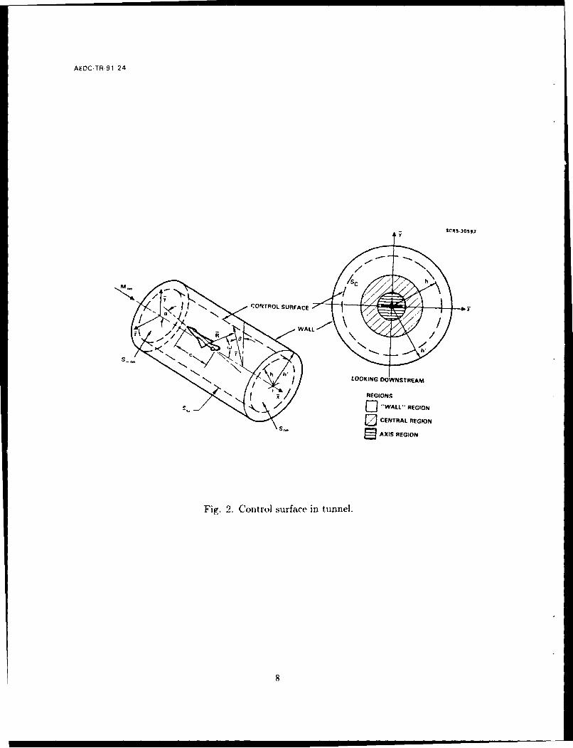
In what follows, the flow over a slender airplane model in a circular wind tunnel testsection will be considered. The main contractual activity in this phase was to computa-tionally solve the wall interference problem (P1) derived in Ref. 29. A schematic of thearrangement is shown in Fig. 2. The interference problem derived in Ref. 29 is associatedwith free jet and solid wall boundary conditions imposed on an interface control surface(shown in phantom in Fig. 2). For this purpose, a secondary limit of a large test sectionradius within the primary Karman Guderley transonic small disturbance limit was used.Only subsonic freestreams are considered in the analysis. In Ref. 29, the flow was shownto have a "triple deck" structure. These decks or zones are shown schematically in Fig. 2.
NTar the axis of symmetry of an equivalent body of revolution havifig the same stream-wise distribution of cross-sectional area as the complete airplane (axis layer), lateral gra-dients dominate. In Ref. 29, the equivalent body was shown to simulate the interferenceof the complete airplane (Area Rule for Interference). Within a "central layer", if a, theangle of attack, and the characteristic thickness, b, are such that a/S = 0(1), as 6 -+ 0, theflow is nearly axisymmetric and can be characterized as a nonlinear line source. Asymp-totic representations for the central and axis layers were derived in which the first orderterms are those associated with the unconfined flow. The second order corrections of theseregions are due to the wall effects. A third region denoted as the wall layer was identified,where the assumption uf small wall perturbations is invalid. Here, other simplificationsapply which represent the slender airplane as a multipole reflected in the walls.
It was shown that the effect of the walls on the flow field is deduced by solving thesecond order problem for the central layer. This consists of the equation of motion, here-inafter referred to as the "variational equation", subject to boundary conditions devisedfrom matching the wall and axis layers.
In the next section, prior to considering the computational solution of the problemP1, some extension of the concepts of Ref. 29 will be applied to a generalization of P1to handle pressure boundary conditions. The numerical solution of this problem was notattempted within the contractual effort.
2.1 Treatment of Pressure Specified Interface Boundary Conditions
In what follows, the flow structure in the region close to the interface, hereinaftercalled the wall layer, will be determined for pressure data specified on the interface. Thisprovides a modified far field for the variational problem from those appropriate to freejet and solid wall conditions. The wall layer as well as the other flow regions have beenidentified in Fig. 2 of Ref. 29 and the inset of Fig. 2. Although the pressure boundarycondition theory was called out as a contractual requirement in connection only withthe high aspect ratio code associated with Task 3.0, the contractor deemed it useful todevelop a corresponding theory for the slender body code written under Task 1.0 in theWork Statement of the contract. This software presently handles solid wall boundary
5

AEDC-TR-91-24
conditions. The formulation of the computational problem for pressure specified boundaryconditions will be given in which the free jet conditions are a special case. This discussionin this section will be restricted to axially symmetric pressure data on the interface. Thislimitation will be removed in a subsequent section.
Referring to Fig. 2, the orientation of a slender model as related to a cylindrical controlsurface delineated in the figure is shown. The set up is similar to that described in Ref. 29.However, a pressure boundary condition is to be -,pecified on the cylindrical interface Sc.These pressures are assumed to be obtained by suitable measurements such as from staticprobes and rails. The pressure distribution is also considered to be an arbitrary function ofthe streamwise coordinate x and in a later section the angle variable 0. Such distributionscar. be associated with the following effects:
" Wall boundary layers
" Noncircular cross section walls such as octagonal and rectangular test sections
o Yaw
" Asymmetric control surface deflections.
Moreover, the pressure specified formulation is relevant to the two variable method,adaptive wall applications, and our recently developed combined asymptotic and experi-mental interference prediction (AIM) method.
2.1.1 KG Theory
For a self-contained account, some of the analytical deveiopments which are commonto the solid wall analysis will be repeated here. The viewpoint will be similar to the solidwall case, i.e., a secondary approximation of large radius h of the control surface (shownschematically in Fig. 2) within the basic approximations of the Karman Guderley (KG)small disturbance model. Thus, the body is represented as the surface
r = Fkx, O) , (2- 1)
within the coordinate system indicated in Fig. 2, with 6 = the characteristic thicknessratio, and overbars representing dimensional quantities.
The asymptotic expansion of the velocity potential 4 in terms of the freestrearn speedU is
-- = +6 20(x, ,O;K,H,A)+... , (2-2)U
which holds for the KG outer limit,
x,r = br,0,K = (1 - M2 )/6 2,H h6/c,A = a/6 fixed as b -- 0, (2-3)
where Mo, = freestream Mach number, K KG similarity parameter, H = scaled heightof control surface, A = incidence parameter. For (2 - 3), the ideas of Ref. 29 and thepressure formula valid on the interface,
CP = -262€z (2-4)
give the following (primary) KG formulation:
6

AEDC TR-91 24
2.1.2 Problem Q:
1 1(K - (-I + + - ( ) i + -00= 0 (2 - 5a)
lim F€f = St (x) 0<X<1( b-O 27" ,0< (-b
¢ (x,0)=0 x> 1 (2-5c)CxH, 0) = f.(x, 0; H) = -Cp 1/26 2 (2 - 5d)
¢(x,gH,o) = .f(x,0; H) (2 - 5d')
Here, S(x) = strearnwise area progression of the test article, S( ) dimensional cross. ctional area, Y = dimensional coordinate in freestr-am dircc;icii, an I S(x) y )/2 ,
where L is the body length. Problem Q above -epresents a generalization of those discussedin Ref. 29 because of the fully three-dimensio,lal nature of the equation of motion (2 - 5a)and in accord with the previous remarks, the more general nature of the external conditions.The latter are given by either (2 - 5d) or (2 - 5d').
2.1.3 Large H Theory
The secondary expansions associated with H -+ o will now be considered. It isanticipated thac the structure of the various Iayers, i.e., Axis, Central, anc Wall layersshow,, ;n Fig. 2, will resemble those for solid walls. Accordingly, these repre-citations are:
2.1.4 Central Layer
0 = O(x,O: + tP1/2(H )01/2(X,r ,G) + yI(H )0i (x , :,) + - "(2 - 6a)
gK= K o + v,(H)K* +... (2 - 6b)
A =Ao + KI(H)AI +... (2- 6c)
which hold in the central limit
x,i fixed as H - oo
These lead to the following generalized hierarchy of approximate equations:
2.1.5 Free Field Approximation
1(1 - (Y + l+ (i 0,) = 0 (2 - 7a)
r
2.1.6 Variational Equations
(K,; - ('Y + 1)0o)OI,2,,. - (h + 1)o.0,/2 + (,;:,/2) + - 1/,, = 0 (2 - 7b)
7
AEDCTR 91 -24
CONTROL SURFACE
LOOKING DOWNSTREAM
REGIONS
WAL REGION
OCENTRAL REGION
ED AXIS REGION
Fig. 2. Control surface in tunnel.

AEDC TR-91 24
(K - ) - (-y + 1)0 0 1 , -, + 1)61,o. + + 0,, = -K1*o., (2 - 7c)7' r
where vi(H) = pI(H) to keep the forcing term in (2 - 7c), and to address the possibility ofadjusting Kj* as a Mach number correction to achieve interference-free flow. The significantcomplication of Eqs. (2 - 7b) and (2 - 7c) over their solid wall counterparts is the presenceof the terms involving 0 derivatives. On the other hand, a substantial simplification fromthe Problem Q is the allowability of factorization and superposition due to the linearity ofthese equations. As will be seen, the angular dependence of the far fields for these problemsinvolve simple factors such as cos 0, cos 20, etc. It is envisioned that this dependence can befactored out, e.g., by allowing 01 = (PI (x, i) cos 0, which gives a two-dimensional equationfor €1. Also to be confirmed by matching is the assertion that the far field for 00 has asimilar structure to that given in Ref. 29.
2.1.7 Wall Layer
The appropriate representation is assumed to be
=o(H),po(xt,rt,) + F1/ 2 (H)p 1 /2 + el'PI + , (2 - 8a)
for the wall layer limit,
xt = /H , rt = /H , fixed asH--oc . (2-8b)
Substitution of (2 - 8a) into the KG formulation giw%,s
O(co) : L[o] =0 (2-9a)
0(f 1 / 2 ) : L[ 1 / 21 (2 -9b)
0((,, f(/H) : L [pi] =(( + 1)vo, - K')po.,. , (2 - 9c)
where
L = * +At AT= a-- rt a 18920 -o x t ,T T- rt Ort rt + rt' 00O2
2.1.8 Behavior of po near Origin
As in the solid wall case, if Rt = y) + 2/H, the source-like behavior,
S0o- S) + 1 ,(2-10)
is anticipated.
From (2 - 5d'), the similarity form,
1f(x,0;H) =-f(xt,0) (2- 11)
H
9

AEDC TR 9124
is appropriate, and leads to the boundary conditions
00(xt, 1,) = f (xt, 0) = f (xf, 0 + 21r) (2 - 12a)
'PI/2,1 (X', 1, 0) = 0 (2 - 12b,)
IfAt = a + 1 a 1 a2
-- ~ ~ 4 )z - r--" + - - O- -
Xt = xt/-K;-
Then (2 - 10) implies
VAt K0 S 21r 6( t2 (2-13)
With the following exponential Fourier transform pair
;;5 = J00e-ikXt odXt
10 e_ eikXt od A
the boundary value problem for i0 corresponding to (2 - 10), (2 - 12a) and (2 - 13) is
V;50 At -k 2 2 -14a)
lim rtd -0 - 1 S(1) (2- 14b)rt -0 drt 27r vfifo
i;0 (1, 0) = 7(0, k) = 7(0 + 27r, k) (2 - 14c)
In contrast to the solid wall case, the decomposition of the solution into the fundamentalsolution M0 and a part M1 that is bounded at X = ±00 as indicated in Eqs. (12) of
Ref. 29 is not required since with the Dirichlet conditions, there can be mass flow throughthe interface to eliminate the solid wall source flow division at upstream and downstreaminfinity. The eigenfunction expansion solving (2 - 14) is
00
io = AoKo(krt) + BoIo(krt) + Z In(krt){1B, cosnO + C,,sinhO} (2-15)n=1
where Ko and I, are Bessel functions, the periodicity condition in (2 - 14c) has been usedto determine the eigenvalues A,, = n, n = 0,1,2,..., and (2- 14b) has been utilized toeliminate the K, for n > 0.
10

AEDC-TR-91-24
Application of (2 - 14c) and inversion gives finally,
I = coskXtdk{ S(1) [;) Ko(k)Ko(krt)]7 (r t)L2'r _- Iok
+ jo(k- f(0,k)dO (2-16)2-~ f o[ k (k,-,) 1 ,
+2; J coskX - )dk 7(', k)cosn(0-0')d0'
The integrals in (2 - 16) are convergent since the Bessel ratios decay exponentially ask ---+ 0 and are analytic as k --+ 0.
As indicated previously, for the analysis in this section, the 0 variation will be sup-pressed. This may be realistic for many practical appiications for nearly circular test sec-tions and interfaces in the intermediate region of slender body theory discussed in Ref. 30.For convenience, the f distribution has been assumed symmetric in X, i.e., f(X) = f(-X),to .btna (2 - 16).* Therein, the exponential transfoms have been expressed in termsof cosine integrals. The analysis can be readily generalized to handle unsymmetrical fdistributions.
2.1.9 Asymptotic Representation of (2 - 16) as R t - 0
To obtain the required representation, the following integrals are considered:
1= cos kX t i(k) dk 2(0, k)dO (2 - 17a)
L I°(krt)K °(k) kXd
12= { Io(k) - Ko(krt)J coskXtdk (2 - 17b)
13 E coskXt I_(k) dk -f(0',k)cosn(0-0')dO' (2- 17c)n=1 00 k 0
Consistent with the assumption of axisymmetric interface pressures, 13 will not b 'onsid-ered here. By approximating Io(krt) and cos kXt as Rt - 0, and term by term integrationof the series obtained, the following approximation for poo results:
S( 1) 2,
0- 47r/k)t + (A0 + B) + (Co + D0 )R P2(cosw)47r .1 1 0 R(2 - 18a)
+O(Rt")
* This restriction will be removed in Section 2.2.
I|

AEDC-TR-91 24
where
A_ = S(1) 0o Ko(k)dk (2-18b)rAo - ;/--o 7r2 10 Io(k)
/3=1 0 dk fo°Bo o(k) f(Xt)cos kX t dX (2- 18c)
Co = -I fo k2 J0 (X t)cos kXtdXt (2-18d)SJ0 Io(k) 0
D = -S(1) j k2Ko(k)dk (2- 18e)o- '-A Io(k)
Here, w is thte scaled analogue of the polar angle defined in Fig. 2 i.e., w cos -1 Xt/Rtand P2 (cosw) is a Legendre polynomial.
The constants given in (2 - 18b)-(2 - 18e) are all given by convergent integrals. Inparticular, 3,, converges if f(k) is bounded as IkI -- oc, and even under milder conditionson f. This results from the potent exponential decay of Io. No problem is encountered ask --* 0 since the integrand is analytic at that point.
The terms involving B0 and Co give the effect of the pressure boundary condition.
2.1.10 Matching
For purposes of matching, the following asymptotic approximations for the wall layerand central region are appropriate:
'TocentraI +62Ao B 0 cosw Co A P2(cosw)}-+ 2 R+ - 2 + (cos 3 w - cos w ) + PR3 (2
+ p/1 1 2 (H)¢I/ 2 + Al (aoR2 P2 (cosw) + aRcosw + a 2 ) +""
as R---* ooU 77i 1 ±(A4P al X + 2 S° - I - '- -- + ( A , + B ) + (C o° + °)R tP (C S L) + "
4 ~~wai1 0-1{fo 0- L 47rRt
+ fl/ 2Bo cosw + +(Co + Do) Rt
+ ,{C [ P2 (CoswL) +- Co + Do] + Co (Cos 3w - cos w)}
asRt --+0(2-20)
where A0 , B0 , C0 , and A are constants that have been previously defined in Ref. 29 with
a corrected value for Co being (-+1) S (I)108r 2
K'/ 1 2
12

AEDC-TR-91-24
Preliminary matching considerations govern the selection of the various elements com-prising (2 - 19) and (2 - 20). The ol coefficient of lil represents a harmonic solution of(2 - 7c). The response to the nonlinear forcing terms (-/ + 1)0o.01., and (-f + 1)01,0o,are (lecaying terms as R - o that are higher order to the order of the matching and canbe neglected. Regarding (2 - 20), 1/2 and ;, the coefficients of el/2 and cl, respectively,consist partially of Xt derivatives of ,0O, such that the multipole expansion has primarysingularities which are source, doublet, and quadrupole forms with their appropriate re-flections. Thus, the reflection of the doullet is an X derivative of the sources, and thequadrupole has the same relationship to the doublet.
For matching Eqs. (2 - 19) and (2 - 20) are written in the intermediate variable
RI . ... (2- 21)
which is held fixed as H -t co. The gauge function q is an order class intermediate between1 and H as H -- cc. This is expressed symbolically as
1 < < T(H) < < H (2-22)
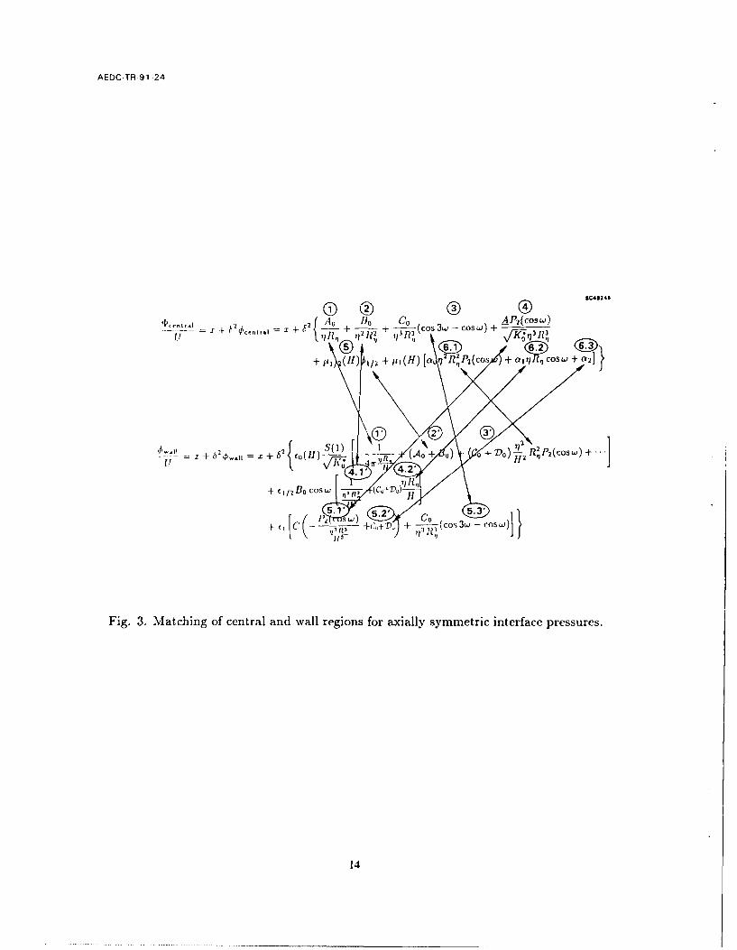
Thus, - 0 as H - cc, and -- -+ 0 as H - c. For axial symmetry of the interfacepressures, the matching process is almost identical to that discussed in Ref. 29. The onlydifference will be the redefinition of certain constants associated with the streamwise inte-grals of the specified pressure data as well as the switchback terms. For understanding ofbasic issues related to the extension to non-axisymmetric interface pressures, the matchingis diagrammed in Fig. 3.
Referring to the figure, the various labeled terms denoted by the circles give thefollowing matchings:
Ao=- o=
0 ('.3 matched
40 +-(0 =6 H3 C
50 0 /11/2 H 12=o+B
PI H3 C1 = o Co+ Do
KG.2 4 a,2' ='a Boao
As will be seen in the next section, the non-axially symmetric case requires additionalterms in the wall, central, and axis layers to deal with the effect of the higher harmonics.
13
AEDC-TR-91 .24
en 2 r. 2 0 1 A P2(cosu) 1434r 6 X +- O + CO (cs3 - cos w) + -
!iI,, (H) £ 2 + I,, { ~ (H) n- Ro + -+ I( Do)Th +~2 w a
4.V 4.2'
+ e(,o cosw R2 (ODO-I
Fig. 3. Matching of central and wall regions for axially symmetric interface pressures.
14

AEDC-TR-91-24
The matching of the central layer and the axis layer proceeds along similar lines tothat given in Ref. 29. All that is required is the essential result for the boundary condition,which is
€, (X, 0) = 0 (2-23)
The expression for the interference pressure remains the same as tlat given in Ref. 29.However, there is an implicit dependence on the interface pressure data through the farfield influence of the terms involving the constants 50 and Co defined in (2 - 18c) and(2 - 18d). Also, the flux of streamwise momentum of the interference field through theinterface must be considered in the calculatiou of the interference drag. The implicitdependence on the interface pressure data is s'iown in the following altered problem P1denoted P2 for the interference potential in the central region 01.
P2:
[Ko - (7 + 1)bo €). (-y + 1+ ' = -K" (2 - 24a)
-" = 0 (2 - 24b)
01 a oR 2 p 2(cosw) +alRcosw+a,, asR- oo (2 - 24c)
where
a0 = Co + Do (2 - 24d)
a, = Boa 0 (2 - 24e)8rboA_
a2 - a0c (2- 24f)
For the free jet case, Co = 0 in (2 - 24d) and B0 = 0 in Fig. 3. Solid wall conditions aremodeled by making ao = NO = boS(1)/V/Ko, with a, = 87rBobo, with b0 = .063409*.
2.1.11 Discussion
Because of the relationship of P1 to P2, the computational algorithm which has beendeveloped for the solid wall case can be used to solve P2 with corrections of the indicatedconstants and the post-processing subroutine DRAG 1 to account for the flux of streamwisemomentum through the interface. Note here that the effect of a2 in (2 - 24c) can beneglected.
* The determination of this value is discussed in Section 2.12.
15

AEDC-TR-91-24
2.2 Generalization to Angular and Unsymmetrical Variations
Summary
In this section, the pressure boundary condition asymptotic analysis given in Sec-tion 2.1 is extended to handle angular interface and unsymmetrical variations of measuredpressure.
Central Layer
With the generalized angular variation at the interface, (2 - 6a) is anticipated to bemodified as
0 = 0 (X,r)+ 112(H) 1, 2 (x,r,6)+P3 14 (H)¢ 3 14 (x,, 0)+pi(H)I (x,f,6)+... (2 - 25)
As compared to (2-6a), (2-25) contains an extra term (indicated by 3/4 subscripts). Thisinsertion is required by matching considerations associated with the more general class ofin~t'rfae Pressure distributions involving angular and asymmetric streamwise variations.
The analysis and results are such that Eqs. (2 - 3) to (2 - 6) remain unchanged.Reflecting the inore general interface distribution the expression for '0 becomes
V0 42(1) ( 01-2) + - + (Q. cosnO 4 Pn sinn8) (2- 26a)47r42 Vr/7- 2
0 47 27rn=1
where
Qi J o(k) e dk (2 - 26b)
Q2 ]Ko (krt)00 =~ In (k,,t)e ' x 27r2 2
Q [C e'~ y( k f 7(0, k) cos n~dO (2 - 26d)
-- I C i (k d)k 7(0, k) sinnOdO (2 - 26e)
Upon expanding the integrands in (2 - 26) for small R, and with considerable algebraicmanipulation, the asymptotic expansions of the integrals can be obtained. The methodol-ogy exemplified in Ref. 29 involves expansion of the Bessel functions for small rt and the
eikXt kernel for small X t and gives a series that can be integrated term by term. Theseintegrals are convergent for the ray limits (Rt -+ 0, 0 fixed) of interest.
16

AEDC-TR-91-24
Collecting results, the desired expansion of po is
.A00
+ .0 + B0 o + AojXto-Rt
+ Sort cos + Tort sin9 +Xt+)7o1rsi0) (2 - 27a)Lo I \ r Xt-o Xtz /
got i cos 20 +Hort sin 29
y 2--Z2 yz
(Co + Do) Rt2 P2 (cosw) +
where the termns shown under those in (2 - 27a) are listed to indicate their correspondence
with spherical 'ernionics and the spherical coordinates are as shown in Fig. 4.
SC50443
Fig. 4. Spherical coordinates.
From the asymptotic expansions, the constants in (2 - 27a) are:
A00 = -S(1)
4oo - K;1) (2 - 27b)
U°S(1) Ko(k) dk B 0 = 1 00 A T -(O, k)dO (2 - 27c)0 27r2 o0 Io(k) 47r _I
1 kdk r 27rAo- 4r2 f,(0,o(k) f 1 (9,k)dk (2 - 27d)
17
AEDCTR-91-24
2.fkrkf'w kdk r2 7r1 = Re 1dY(k) -cosOdO o= Re J_ 11(k) 1 sinOdO(2 - 27e)
Eoi 2 Re i-o k,(k , fcosOdO , = 2Re i (k) f sinOdO
(2 - 2 7 f)S(1) k2Ko(k) 1 0 k2dk I -C0 - 4r V - - I - ok dk , :Do = - 8 - - Io ) TJo( - 2 g
47r2\/-70- iIo( k) 8i2 l ()1
go = 1Re k I(k) 1 Ifcos2OdO , ?io -- Re] -oy f sin2OdO
(2 - 27h)
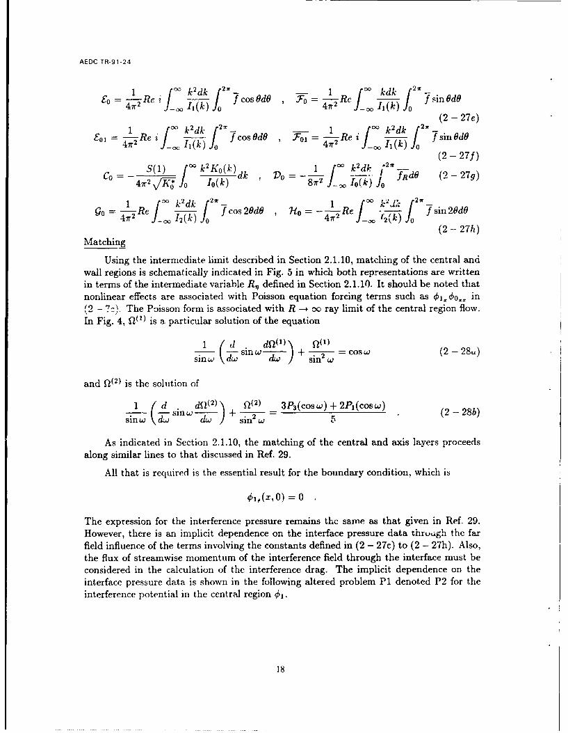
Matching
Using the intermediate limit described in Section 2.1.10, matching of the central andwall regions is schematically indicated in Fig. 5 in which both representations are writtenin terms of the intermediate variable R,, defined in Section 2.1.10. It should be noted thatnonlinear effects are associated with Poisson equation forcing terms such as 01.0o., in(2 - ). The Poisson form is associated with R --* oc ray limit of the central region flow.In Fig. 4, fQ(') is a particular solution of the equation
1 d .&d2(0)' Q(1)sinw u;-cs (2 -28u)
sinw \dw +- + sin 2 W - CO( )
and Q( 2) is the solution of
1 (ds dQ ()\ Q(2) = 3P3 (cosw)+2P,(cos w)
sin + 2 - 5 (2-28b)
As indicated in Section 2.1.10, the matching of the central and axis layers proceedsalong similar lines to that discussed in Ref. 29.
All that is required is the essential result for the boundary condition, which is
€1,(z,0) = 0.
The expression for the interference pressure remains the same as that given in Ref. 29.However, there is an implicit dependence on the interface pressure data through the farfield influence of the terms involving the constants defined in (2 - 27c) to (2 - 27h). Also,the flux of streamwise momentum of the interference field through the interface must beconsidered in the calculation of the interference drag. The implicit dependence on theinterface pressure data is shown in the following altered problem P1 denoted P2 for theinterference potential in the central region 01.
18

AEDC-TR-91 -24
PRES-URES SPECIFIED ON INTERFACE:
+ A-I RP iZIv: S 0- .Tr d~h~lO4U + P2 (CosW)1
,I-I=~l S( +A + Vo-4+ Cos + (CO-i )711 ' COSW)
+ "snw Cos 0+Y .l1O 2 sin' Ocos2V -4-2 osin29)
+ _iB + ( 00(0 + +~ Qi i(E co 6 + 2Y 0 sin 6 ) + +Ad,~
Fig. 5. General case of matching of central region and wall layers.
19

AEDC-TR-91-24
P2:
[Kos - (-I + 1)0o,]9~ -Pi, + ±)Qo 61, + (roi. = -K" 0 , (2 29a)
,,0) = 0 (2 - 29b)
4 _- 2 o (cLs.) + Cos Sill: I1c FoS0 20Sing22
" 2 (il W 3Cos 20 +A4sin 20)(2 - 29c)
"+R{ COS W+ sin iw (A5 sin 0:Acrcos) }+A 2 +" asR--c.
where by Fig. 5, with B and C defiled in Ref. 29
Co + Do t2 - 29d)
41 - 2BAo (2 - 29e)
,2 =2CCI 2B (Co + Do) (2 - 29f)
3 - (2 - 29g)
xi Ro (2 - 29h)
A5 - 7, (2 - 29i)
A6 = E01 (2 - 29i)
2.2.1 Discussion
The problem (2 - 29a)-(2 - 29c) is the generalization of the Problem P2 given in Sec-tion 2.1.10 accounting for asymmetries in the streamwise distribution of the interface pres-sures as well as angular 0 variations. These effects are given by the terms marked as (1)
- (3) in (2 - 29c). They represent averages of the early harmonics which to this order isall that the far field is sensitive to. The specialization to the free jet case is obtained bysetting Do = go = 7"o = Cl = Fo01 = 0 in Eqs. (2 - 29).
2.3 Shock Jump Conditions
An important element to be considered in the numerical solution of the Problem P1
referred to in the previous sections is the satisfaction of the shock jump conditions. For
20

AEDC-TR-91-24
the free field case, these relations are satisfied by the divergence or conservation formof the Karman Guderley small disturbance equation. These give the Rankine Hugoniotjump conditions. They are satisfied using type sensitive shock capturing schemes such asthose originally developed by Murman and Cole in Ref. 31. On the other hand, the wallinterference corrections related to the Problem P1 have to be satisfied by use of explicitrel.tions. These have been derived for the high aspect ratio transonic lifting line theoryfcmulated in Ref. 32. These relations will be derived for axisymnietric 3ow in this section.
Referri:g to Fig. 6, conditions across the shock front denotea as S will be discussed.!1i., surface is given by
S=x-g(F)=0 , (2-30)
where = 6r, and consistent with the Problem P1 delineated in Ref. 29, axial symmetry isassumed. The Problem P1 describes the wall interference flow away from the walls on thei.xis of symmetry of a cylindrical test section. The velocity potential in this zone, denotcdby $ , is given by the asymptotic expansion SC84-29502
n
-(r) SHOCK
U
SHOCK SURFACEX
Fig. 6. Orientation of shock surfaces.
X+ 200(X, F) + L + 1--1(X,,) + ••• ,(2-31)
where U is he freestream speed, the Oi are perturbation potentials, a is a constant, H isthe wall height in units of the body length, and b is the confined body's thickness ratio.The secondary expansion in the braces in (2 - 31) is an approximation for the perturba-tion potential 0 which is governed by the Karman Guderley transonic small disturbanceequation (2 - 5a), with -2 assumed zero.
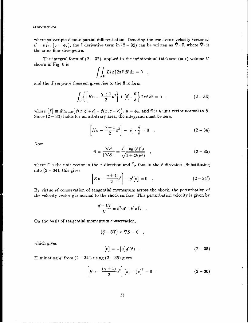
Equation (2 - 5a) can be written in the divergence form,
L{¢}=t +¢ +102} 12j K - + ( ) = 0 ,(2-32)
21
AEDC-TR-91-24
where subscripts denote partial differentiation. Denoting the transverse velocity vector asv = vl , (v = 4€t), the i derivative term in (2 - 32) can be written as V i, where V. isthe cross flow divergence.
The integral form of (2 - 32), applied to the infinitesimal thickness (= f) volume Vshown in Fig. 6 is
I JvL{}2rd&dx=O
and the d;veigence theorem gives rise to the flux form
L[Ku -+u2] +]+ [ ] " 2rf d=0 , (2-33)
where [f] -n,-o{f(x,g + ,) - f(x,g -,E)}, u = 0, and i is a unit vector normal to S.
Since (2 - 33) holds for an arbitrary area, the integrand must be zero,
[Ku -+u2] + [ ] " =0 (2-34)
Now VS _ - 6 g'(i)1i.ii - , (2-35)IVSI V/1 + 0(62)
where F is the unit vector in the x direction and fl that in the f direction. Substitutinginto (2 - 34), this gives
Ku - --+1u2] _ g'[v] = 0 (2 - 34')
By virtue of conservation of tangential momentum across the shock, the perturbation ofthe velocity vector is normal to the shock surface. This perturbation velocity is given by
_ i-62ur+ 63VfU
On the basis of taingential momentum conservation,
ur) x VS = 0
which gives[v] = -[u]g'(, ) (2-35)
Eliminating g' from (2 - 34') using (2 - 35) gives
LKu + +1) 2][u] + [v]2 =0 (2-36)
22

AEDC-TR 91-24
Since tangential momentum is conserved, the tangential velocity component to theshock is continuous across it. Upon tangential integration, and disposing of an unessentialconstant, the following relation is obtained
[] =0 (2-37)
Equations (2 - 36) and (2 - 37) lead upon substitution of the asymptotics into the jumprelations for the approximate quantities appearing in (2 - 31). To obtain a determinateset of quantities, the shock's representation is assumed to be in the same form as that for€, i.e.,
g -: go( ) + I g1 1 2() + 1g +" (2-38)
Denoting f as a quantity of interest which has the same asymptotic form as €, on the basisof (9 - 38) And Taylor's expanbiukn,
f(x,g) =fo(x,go) + 1 (f1 1 2 (x, go) + g11 2fo(x,go))
H2g 2 1 (- 39)/2 fo..(X, go) + - Y(lX,9go) + g A. (X, go)) (
H2 .,,
By virtue of (2 - 39), substitution of the expansion (2 - 31) into (2 - 36) gives the approx-imate shock relations which are:
0(1) (K- -t + luo uo + [Vo1 2 = 0 (2 -40a)
]Kuo- 2 [u + [(K - (- + 1)uo)ul]
+ 2 [vo] v = -gi{ [Iuo] [(k - (-y + 1)uo)uo] (2-40b)
+[Kuo - + 1Ul[uo ]
L 2 ]0
+ 2[vo] [vo] }
where uj - Oi. and vi = O where i is equal to 0,1. The quantity 91/ 2 can be shown tovanish on the basis of (2 - 37) which with (2 - 39) leads to the additional set of relations:
0(1) : [0] =0 (2 -41a)
o(H- 3) : [01] = -g [00 ] (2 - 41b)
It should be noted that the O(H - 1 ), O(H - 2 ) equations obtained in the process leading toEqs. (2 - 40) are vacuous.
23
AEDC TR.91-24
Equations (2 - 40) and a vorticity relationship to be derived in the next section
complete the formulation necessary for the computational solution.
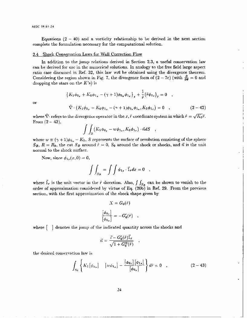
2.4 Shock Conservation Laws for Wall Correction Flow
In addition to the jump relations derived in Section 2.3, a useful conservation law
can be derived for use in the numerical solutions. In analogy to the free field large aspectratio case discussed in Ref. 32, this law wJlI be obtained using the divergence theorem.Considering the region shown in Fig. 7, the divergence form of (2 - 7c) (with o = 0 and
dropping the stars on the K's) is
1
{K,710o + K 0p 1 . - ( + 1)0p0.,1} + = 0r
orV" (K 1 0 -i- I¢, - (- + i)Oo,0.,K01,) = 0 (2- 42)
where V. refers to the divergence operator in the x, i coordinate system in which f = !X/10f.
From (2 - 42),f (Kl Oo,- w 0., Ko, 0,)'n dS,
where w ('y + 1)0o, - K 0 , S represents the surface of revolution consisting of the sphere
SR, R = R 0 , the cut SB around i = 0, So around the shock or shocks, and il is the unitnormal to the shock surface.
Now, since (x, 0) = 0,
I LSB IJff0,. jdwhere 1f is the unit vector in the direction. Also, f fsR can be shown to vanish to the
order of approximation considered by virtue of Eq. (20b) in Ref. 29. From the previous
section, with the first approximation of the shock shape given by
X Go(i)
[€0,] _ -
where denotes the junip of the indicated quantity across the shocks and
V 6 + -G (02
the desired conservation law is
[{' [ UJ [11,0iJ - 0o[] =d 0 , (2-43)
24

AEDC-TR-91-24
A SC8S.30608
SR R
/1 S
L - jb x
Fig. 7. Regions appropriate to shock conservation laws.
25

AEDC-TR-91-24
where So is the shock surface.
2.5 Regularization of the Problem for the Correction Potential 01
To avoid the singularity at oc, the problem P1 in Ref. 29 is transformed by subtractingoff the far field for 01. Accordingly, the variable ki is introduced in P1, where
1= - OFF (2-44)
.dfere,1
M[01] - (Ko -(^t + 1)0oo. = -t + 1o.€, + ( ,)=-K,Oo,. (2 - 45a)
r
andlim 01, =0 (2 - 45b)
Noting that (for solid walls)
€1 - OFF = bO'oR2P2(cosw) - 87rbnBoR cosw (2 - 45c)
as
f= 2 + f2 .- oC
and
wFF 0 (X - 2) + 87rboBoX (2-46)
where
1' =S(1)bb"C 0000
47rB 0 = -S(1) + S(x)dx + 7r(-y + 1) dx 20d&0 -00 JO
w = polar angle defined in Fig. 1
S(x) = model cross sectional area
R = polar radius defined in Fig. 1
From (2 - 44) and (2 - 46), (2 - 45a) and (2 - 45b) become
Mr[:1 2(-y + 1)0ob M( +(0.. 4ox + 87rbOBO K,1 (2 -4a
lim 0 0 (2 - 47b)
-*0 as R - oo (2 - 47c)
26

AEDC-TR-91 -24
where R =-bR.
The slender body interference code will use the regularized form represented by Equa-tions (2 - 47).
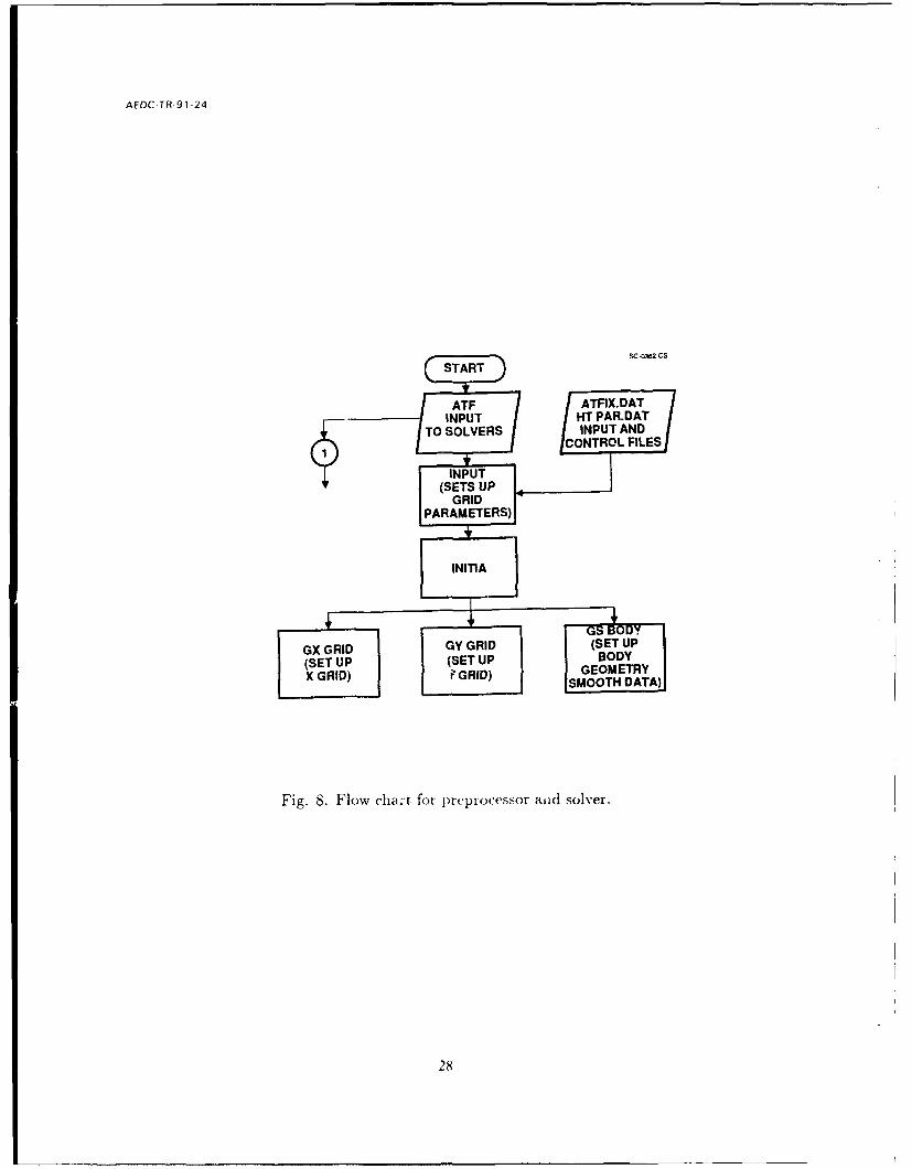
2.6 Basic Code Modules
Figures 8 show flow charts which give an overview of the interaction of the functionalmodules to be used in the design of the wall interference code under Task 1.0. Thepreprocessor ATF sets up the grid and inputs other parameters through the subroutinesINITIA, INPUT. The input georaetry data is read in from the disk file. The solver STINT25has primary subprograms denoted as RELAX1, OUTFNL, SONIC, DRAGI used to solvethe zeroth order flow problem and RELAXV1, OUTFNL1, and DRAG1 for the variationalproblem for q 1. RELAX1 and RELAXV1 are modules which respectively are the principalsuccessive line overrelaxation routines which serve the purpose of solving the tridiagonalsystem for the free field and the interference problems. The tridiagonal solver is denoted asTRID. RELAX1 and RELAXV1 include special treatment of far field, internal, boundary,and shock points with appropriate type sensitive switches. SONIC determines subsonicand supersonic zones, and OUTFNL and OUTFNL1 provide the basic flow and interferencepressure fields as well as the quantities gi defined in Ref. 29 necessary to compute free fieldand interference drags. These are computed in DRAG and DRAG1, respectively. Therelationship of the flow solving modules is shown in Figs. 8.
2.7 Upstream and Downstream Far Fields
For slender test articles that are sting mounted inside solid walls, the flow at greatdistances from the model behaves as a confined source in accord with the analyses given inthe previous sections. Referring to the cylindrical coordinate system indicated in Fig. 9,far field behaviors were worked out in certain "ray limits" in which if R = v/T _+r andcosw = z/R, R --+ 0 for 8 fixed. The case w = 0, or 7r, i.e., x - +oo however is degenerateand requires special treatment and had not been analyzed.
For a properly posed numerical simulation of the finite height case, the structure ofthis flow must be properly modeled. This can be achieved using the Divergence Theorem.
If x is the usual dimensionless coordinate in the freestream direction depicted in Fig. 9,then the transonic small disturbance formulation gives the following equation of motion
1 (7+AO -- dxx + Z (oi:) = lxOxx (2-48)r VKg
where K = (1- M')/ 2 , Al, = freestream Mach number, 0 is the perturbation potential,and X = x/v/K-. The slender body boundary condition is
im 0 S'(x)lim = - (2-49)F-o r 27r '
where S(x) is the cross sectional area distribution for 0 < x < 1, and S'(x) is withoutgreat loss of generality assumed zero for 1 < x < co, (constant diameter sting).
27
AEDC TR 91-24
G D sc-aw-csP O' D
ATF A FIX AINPUT T i DATH T I
TO SOLVERS N UT ANDCONTROL FILES
INPUT(SETS UP
GRIDPARAMETERS)
INITIA
7 GS HO
GX GRID GY GRID (SET Up
(SET UP (SET UP BODY
X GRID) FGRID) GEOMETRYSMOOTH DATA)
Fig. 8. Flow cha:-t for preprocessor aiid solver.
28

AEDC-TR-91-24
SC 0360-CS
S SOLINP. DATATFBOPT. DAT
ATFBOPI"V. DATx, 1 VECTORS, DX,GAMM1, GAM,
PI, IMAX, JMAX, PHI, PLS, SBODY,
PLS1, TAU, ETC.
STINT25MAIN DRIVER
RELAXI, RELAXV1(SOLVE DIFFERENCE
EQS) FOR 0th ANDPERTURBATION FLOW
COMPUTECOEFFICIENTS
Fig. 8. Flow chart for preprocessor and solver (continued). N in the notation STINTN denotesthe Nth version of the main driver.
29

AEDC-TR 91-24
-,C 0361 CS
(SONILVEGORG
Fig.~~~~1 8.Fo hrtfrprIAoesran ove cncue)
30TE

AEDC-TR-91-24
A control cylinder is considered consisting of the walls (SH), an internal surface bound-ing the model near the axis, (S,), and the inflow and outflow faces (S-,,) and So., respec-tively. Accounting for the impermeability of the walls expressed as
OfI 0 (2-50)
the divrg-nce theorem when applied to (2 - 48) gives
jJp cV = JLI HSOS0 f LdS =27r jH Fd ) ; X,s.+s+_ a o0 2W- b X •
(2 - 51)where V denotes the volume of the control cylinder. Evaluating the terms in (2 - 51),
[ adS = lim] dO 00 ad 2r] ''dX = S(1) (2-152).I, dn .0 -o d" 2,"
From (2 - 50),
f dS=O (2-53)JSflan f= H
For a slender configuration, we assert that as in the subsonic case, the lift effect producesa Trefftz plane (x = oo) flow component that can be represented as an infinitesimal spanvortex pair reflected in the walls. This pair is the Trefftz plane projection of the trailingvortex system from the body. Superposed on this flow is an outflow due to the sourceeffect. A similar outflow occurs at x = -00. Accordingly, we are led to the asymptoticinflow and outflow conditions
qS-CFFx +f(,,) as x - oo (2 - 54a)
( = i sino'z= cos a)
h -CFFX as x - -oo (2 -54b)
where f( , z) is related to the lift, and the constant factor CFF appears in the mannerindicated in order to preserve the anticipated symmetry of the apparent source flow fromthe sting-mounted, finte base area model. In this connection, it is important to note thatEqs. (2 - 54) are exact solutions to the nonlinear small disturbance equation (2 - 48). Thisis true even for f(g, i), since it satisfies cross flow Laplace's equation. It should be notedthat the inflow and outflow conditions to be specified at x = ±00 are independent of theform of f.
Fcom (2 - 54), it is clear then that
+s_ dS = 2rCFFH2 (2-55)
31

AEDC-TR-91-24
/ H
Fig. 9. Model confined by solid cylindrical walls and control volume.
The last term to be evaluated in (2 - 51) is the right hand side, which isL 2VKdX (p2) dX = (; ~ JH {€ (oo, )- €3c(-oo,i )} d
which vanishes by virtue of (2 - 54), as a milder condition of symmetry of the axialcomponent of the far upstream and downstream flow. From this, as well as (2 - 51)to (2 - 55), it follows that the inflow and outflow conditions are,
S( 1)
6 " S-2 as x-4+oo , (2 -56)
i.e., the apparent source strength is proportional to the body base area. Equation (2 - 56)is used in the numerical simulation of the flow field.
A complete asymptotic expansion based on the eigenfunction expansion for a confinedpoint source given in Ref. 29 can be used to obtain refinement of (2 - 56) and treat thetransonic case. From Green's theorem and the properties of the Green's function G, theperturbation potential in the confined incompressible solid wall circular cross section
case is
=- 2 2 Ixz- S'( )d + 2xH S'() - (2-(A5)6
22rr 2
i~. teapa Jn oucsteghiprotonlote boybaeoxa Eqato (2 -A 56)
is sedin he umeica smultio oftheflo fil2

AEDC-TR-91-24
where the summation is over the eigenvalues A. which solve the following secular equation
J(AH) = 0
Thus,A1H = 3.8317
A2H - 10.1734A3 H = 13.3237
From these eigenvalues, it is clear that for moderate H, the confined flow decays muchmore rapidly upstream and downstream than the free field, with the former demonstratingexponential relaxation to the freestream and the latter, algebraic behavior.
Based on these considerations, and extension to compressible flow which introducesa nonlinear volume source the expression for the asymptotic upstream and downstreambehavior is
2rH2 K K K d 0 0. (2-56')
+ TST as x -*±oo
where TST = exponentially small terms which are
0 (e-% I l ) as IxI -oo
V =j S()dz
The last term in (2 - 56') represents the average kinetic energy of the horizontal pertur-bation of the flow.
2.8 Difference Equations for the Wall Interference Correction Potential
A successive line overrelaxation (SLOR) algorithm for the large height correctionpotential has been coded. The initial approach is to use modifications of type sensi-tive switches developed by Murman and Cole3 1 , and pseudo-time operators devised byJameson 33 as well as generalizations of the procedures developed in Ref. 34. Results to bediscussed for the full nonlinear finite height theory algorithm show good convergence fortransonic Mach numbers.
The basic code modules to treat this problem have been flow charted in Fig. 8. Prin-cipal modules are RELAX1 and RELAXV1 which are used to solve the discretized formof Eqs. (2 - 47) by nonlinear iteration and SLOR. Some highlights of our approach willnow be outlined.
33
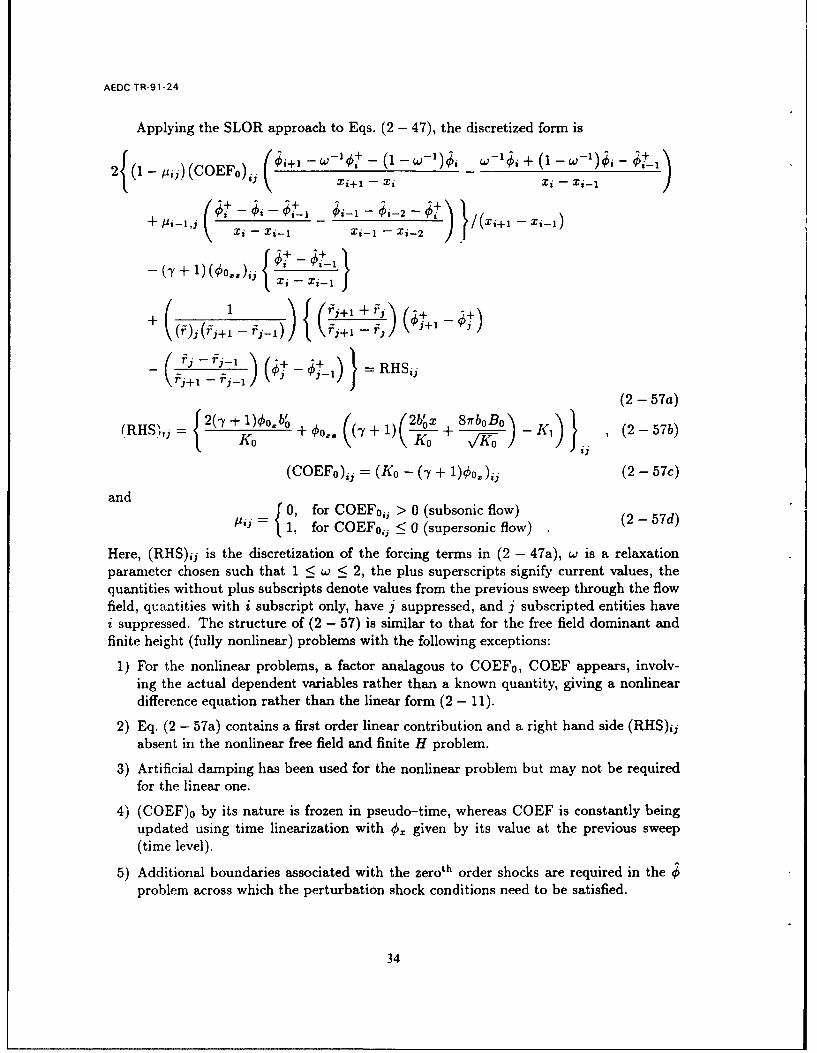
AEDC-TR-91-24
Applying the SLOR approach to Eqs. (2 - 47), the discretized form is
2\(1r-)-')+, woj + ( 1-,
(2 - 57a)
+ I K0 I€0)= (+l+ I)\ + + 0 81rbOBO) (257b)
(COEF0),, (K - (7 + 1)¢0,) 1 (2 - 57c)
and 0, for COEF0,, > 0 (subsonic flow) (2 - 57d)/ =1, for COEF0.j < 0 (supersonic flow) 2
Here, (RHS)ii is the discretization of the forcing terms in (2 - 47a), w is a relaxationparameter chosen such that 1 < w < 2, the plus superscripts signify current values, thequantities without plus subscripts denote values from the previous sweep through the flowfield, qucatities with i subscript only, have j suppressed, and j subscripted entities havei suppressed. The structure of (2 - 57) is similar to that for the free field dominant andfinite height (fully nonlinear) problems with the following exceptions:
1) For the nonlinear problems, a factor analagous to COEF0 , COEF appears, involv-ing the actual dependent variables rather than a known quantity, giving a nonlineardifference equation rather than the linear form (2 - 11).
2) Eq. (2 - 57a) contains a first order linear contribution and a right hand side (RHS)iiabsent in the nonlinear free field and finite H problem.
3) Artificial damping has been used for the nonlinear problem but may not be requiredfor the linear one.
4) (COEF)o by its nature is frozen in pseudo-time, whereas COEF is constantly beingupdated using time linearization with 0. given by its value at the previous sweep(time level).
5) Additional boundaries associated with the zeroth order shocks are required in theproblem across which the perturbation shock conditions need to be satisfied.
34

AEDC-TR-91-24
Note, for bodies with pointed tails, Eq. (2 - 57b) specializes to
(RHS)ii = 8irboBo(y + 1)(qo,),, (2 - 57Y)
The tridiagonal system for €k is then
Bjj + Dj( j + A¢j~+j = C), j = 2,3,.. ,JMAX- 1 (2-58a)
D=- 2{(10 .Pj)(COEFo) +I )ij (Xi+l - xi Xi - Xi-i
- i-lj (COEFo)i-l, 1 G i - xi- 1 + Xi-1 Xi-2 }/(xi+1 - x- 1 ) (2 - 58b)
(7 + l) ~~ ij+i +iz +j f + F-ZL}
xi - Xi-1 -i (fi+ - -) (+8+ j + r - ri_)
A, = 1 Fj+ fi' (2 - 58c)
fj(Fl -Fj1)G -', (i- w),-Aj= 1 F1+j + fj) (2 - 58d)
Cj =-2 (1 - J 1 ) (COEFo)ij /+ (1 - - ) - (1
- .. - ( ii i i + --
(2 - 58e)
At the body, j = 2, and the previously indicated boundary condition, €1, = 0 implies
D2 = D > 2 + 1 (2-59a)r2r3
B 2 = . (2 - 59b)
Also, A 2 and C2 take their specialized values at F = F2 (with j = 0).
In (2 - 58) and (2 - 59), the /pj are designed to provide the necessary type sensitiveswitching and implementation of Murman's shock point operator defined in Ref. 35. Thisbehavior is essential not only for the zeroth order solution but the variational one as well.
Subsequent sections will describe the scheme of shock fitting that interacts with thedifference equations (2 - 58) and (2 - 59).
2.9 Finite Height Application of Zeroth Order Code
As indication of an application of the zeroth order part of STINT25 calculated byRELAXI, an equivalent body of revolution representative of a transonic/supersonic
35
AEDC-TR-91-24
blended wing fighter configuration was computed in a solid wall wind tunnel. The cross sec-tional area progression of the model is indicated in Fig. 10 which shows curvature changesassociated with such geometrical features as wing-body intersections, canopies, and inlets.One purpose of this study was to explore aspects of the application of the code to realisticairplane geometries.
0.12 x 10 5 -
0.9 x 10 4
NC
0.6 x 10 4
x
U)
0.3 x 10 4 -
0.0 I ! I I I
-200 0 200 400 600 800 1000
x (in.)
Fig. 10. Area distribution of blended wing fighter configuration.
As an indication of the flow environment for subsequent wall interference studies,Fig. 11 shows the pattern of isoMachs over the configuration associated with Fig. 10 in afree field at M.. = .95. These results could be practically obtained using the nonlinearanalogue of the difference method associated with Eqs. (2-57)-(2-59) on a VAX computerin a CPU limited Fast Batch or interactive environment. The grid utilized 194 points inthe x direction with uniform spacing over the body and logarithmic stretching aheadahid behind. In the f direction, a similar geometric progression spacing was used with
36

AEDC-TR-91-24
50 points. Nominal convergence* typically was achieved between 500 to 1500 sweeps, withmore sweeps required at the higher transonic Mach numbers.
2/15
r 1/15 r
-4/3 -2/3 0 2/3 4/3X
Fig. 11. IsoMachs over blended wing configuration in free field, M"f = .95.
The complexity of the flow structure evident in Fig. 11 is to be associated with themultiple inflection points of the area progression and the possibility for envelopes to formin the steeply inclined wave system. In Fig. 11, a shock is formed near about 2 of the
3body length from such an envelope process.
Figures 12 and 13 illustrate the Mach number and surface pressure distributions atthe same freestrean Mach number for the free field environment and a solid wall confinedcase. To obtain a nominal simulation of the free field, the upper computational boundaryj = JMAX was placed at H 1.3 and homogeneous Dirichlet conditions were imposedthere. Homogeneous Neumann inflow and outflow conditions at x = -oo were also pre-scribed. For the solid wall simulation, H m 0.66 was utilized. Homogeneous Neumannconditions were used at j = JMAX and Eq. (2 - 9) applied at x = ±0o.
* Defined as max I<i<IMAX - 1i= 10-.
I( 3 <JMAX
37

AEDC-TR-91-24
1.4-01.4H = 1.32 "'FREE FIELD"
1.2- (NO FREESTREAM
PERTURBATIONERRMAX - 0.00004
w" 1500 ITERATIONS)""1.0-1.0 -HOMOGENEOUS DIRICHLET
C CONDITION AT UPPERU 0 COMPUTATIONAL BOUNDARY
S0.8
J 0 H = 0.66 "CONFINED":<:0 030 FREESTREAM PERTURBED
00.6- 0 ERRMAX 0.00008
1300 ITERATIONS
0.4 /X/ I///=X///////// __
0.4
0.2 1I I I0 0.2 0,4 0.6 0.8 1.0
X/L
Fig. 12. Finite height solid wall interference effect at Af = .95 on blended fighter con-figuration equivalent body - Mach number distribution over body.
38

AEDC-TR-91-24
0.6- 06H = 1.32 "FREE FIELD"(NO FREESTREAM Y)PERTURBATION)ERRMAX = 0.00004
0.4- 1500 ITERATIONS)
0 H = 0.66 "CONFINED":FREESTREAM PERTURBED (9ERRMAX t 0.00008
0.2 1300 ITERATIONS
0 0
// 0 00
0
L
-0.61 I I0 0.2 0.4 0.6 0.8 1.0
x/L
Fig. 13. Finite height solid wall interference effect at Moo = .95 on blended fighter con-figuration equivalent body - surface pressures.
39
AEDC-TR-91 24
From the figures and in accord with simple one-dimensional gasdynamic reasoning,the constrictive effect of the solid walls is to exaggerate the effect of stream tube areachanges associated with body area changes.
An experimental validation was performed of the 0th order solver RELAX1 basedon one of the variable blockage ratio tests of a blunt nosed model (B-3) in the Langley8 and 16 foot tunnels, reported in Ref. 36. The test section was slotted and slatted aswell as uctagonal in shape. For such a blunt body which locally violates small disturbancetheory. fhe agrreerpnt with the data is surprisingly excellent as shown in Fig. 14. For thiscorriuaL'ion, the special improved accuracy boundary discretization proced-ii: describcdin tht. next section was used. The quality of the comparison is believed to be partiallyattributable to this improvement.
2.1A Improved Accuracy Procedures for Numerical Treatment of lqody BoundaryConditions
In the finite wall height application of the code, the interference pressures are com-puted as the difference between the confined and free field pressures. The numerical trun-cation error is a larger percentage of this difference than of either of the former quantities.This fact puts a greater demand on numerical accuracy than has been stressed in state ofthe art codes. Accordingly, all error sources were evaluated. Some items considered withinan incompressible and subsonic framework were:
1. Accurate treatment of boundary conditions on axis of equivalent body.
2. Proper application of upstream and downstream far fields.
3. Need for double precision on shorter word length computers such as the VAX to handlehigh frequency errors propagating on fine grids for large iteration counts.
4. Treatment of nose and tail singularities.
The techniques apply directly to the transonic case. Moreover, study of subsonic flowsis particularly useful because of the availability of closed form analytical solutions to checkthe numerics.
The second of Figs. 8 shows the subroutine RELAX1, which solves the tridiagonalsystem representing a discretized approximation of the transonic small disturbance partialdifferential equation of motion (TSDE) (2 - 5a). It contains a special procedure whichdeals vith the boundary conditions. These are satisfied by incorporating the conditionof flow tangency at the body into the discretization of the vertical perturbation velocityflux gradient. In the nonlinear difference equation for the free field flow (2 - 57a), thiscorresponds to an approximation fulfilling the role of the terms in the braces on the lefthand side near the equivalent body of revolution (EBR) line of symmetry, (x axis). Onescheme employed is associated with Eqs. (2 - 59a) and (2 - 59b).
Figure 15 is a schematic representation of the nodes relevant to the boundary points.In the finite height case, this treatment is made more difficult because the perturbationpotential is logarithmically singular as the scaled radial coordinate tends to zero. Existing
40

AEDC-TR-91-24
0).2 r . . .. ... _ __ _ __ __ _ __ _ __ _
0----0--0 0 0 0
/
o COUCH: LANGLEY 16' SLOTTED TUNNEL
-0.3 -CODE (SOLID WALL B.C.)
-0.55 -
00
-0.8 -
0 0.25 0.5 0.75 1
Fig. 14. Validation of RELAXI code against Couch experiment, B-3 body, M = .99.
41
.AEDC-TR-91-24
free field codes familiar to us do not properly deal with this singularity. Whereas thislimitation may be of moderate consequence to the prediction of free and confined nr-:. ,'cs,in accord with the previous remarks, it is absolutely crucial to the treat:.., • of interferencepressures and testing of the variational equation solver. Accordingly, attention was given tothe development of a scheme that accounts for the singularity in the boundary treatment.
r
j= 3
5
22 0
3
0 x.-x
Fig. 15. Nodes in vicinity of axis.
Referring to Fig. 15, the discretization of the third term,
1T : -OO (2-60)
r
in the TSDE will now be discussed. This is the vertical flux gradient previously indicated.Shown in the figure are the first 3 (j) vertical node points as well as 1 node points. IfFi,j = 1,2,.-, JMAX represent the j mesh points,
rj+1/ 2 = (rj+l + ri)/2, (2-61)
we consider (dropping the subscript zero on . and the tildes on r), the discretized versionof T - T,, given by
T2{! (r1r)r} (2-62)
Using the half node points in the vicinity of the x axis
T2 1 (rOr) 5 /2 - (r€r) 3 /,2 (2 - 63)r 2 r5 / 2 - r3/2
42

AEDC-TR-91-24
The essential new idea is that a "regularized" version 4 of the perturbation velocity po-tential 4 is introduced, where
= SX) Inr
2r (2-64)S'(x) = streamwise (x) derivative of the EBR area progression.
The logarithmic sing-ilarity is represented by the second term in (2 - 64). Numerical differentiation of 6 in the r direction is then accomplished by differentiating 4 as the suiof a numerical approximation of its regular part and an analytical evaluation of the loge-rithmically singular coniponent. The truncation error which would have normally becomelarge due to the infinity on the axis will be substantially reduced using the differentiatior.of the linear polynomial representing the bounded quantity 4.
In accord with these ideas, the terms in (2 - 63) can be evaluated as follows:
(r4r)5/2 (r3 -t-r2) r3 -r2 + 2 ((3+2)/2 2 ( ) 2 +
2 r, 3 - r2 - r +. ln2/2 22 r3 - r2 27rs(=2_(r 3 + r2) 03a-042 - S( In r3/r 2
s'w +, S4 ,- 2 r3 -r2 27 r(2 - 65a)
(r4)r) 3,, 2 =r 3 /2 r13/2 + 2wI(X) J r323/2 /2 27r
(- -1 ( r2-g(x) +( _. (2-65b)2 - r 27r
where the fact thatS'(x) + r -() In (2-66)
T2 - 22has been used in (2 - 65b). Noting that r1 = 0, and collecting results,
r2( r3 - r2 (2-67)
I[ S'(x) Inr X
r3 2 27r
Accordingly, the tridiagonal system discretizing TSDE
Bii-..+D 1 4i)+Aq$i + i =C , j=1,2,..,JMAX
at j = 2, has in accord with (2 - 67),
B2 = 0 (2 - 68a)
Aj> 2 (2 - 68b)
D2 = D j > 2 1 = 2 (2 - 68c)
C2 = Sj )=2 + [r3 + r2 -Inr2 g(X) (2-68d)21rr 2 r3 21r r3 -r2 r 2
43

AEDC-TR-91-24
In the computational implementation, g(x) is initialized as zero and then updated eachiteration using (2- 66). For (2- 68d), g(x) is "time linearized" from the previous iterationwithout relaxation. As an additional refinement, it is useful to note that the three dotsin (2 - 66)
_ S"'(x)4(r 4nr r2)
in incompressible and subsonic Prandtl Glauert flow, and is an O(S.'(x)r2 In2 r) expressionat transonic Mach numbers. The updated g is computed using linear extrapolation as
(2-69)r3 r2\ ]
Numerical experiments show that this produces results equally acceptable to those from anasymptotic approximation based on previously mentioned higher order terms proportionalto S"'(x) when S..(x) is known analytically. For tabular S(x) input, the linear form (2-69)is preferred due to significant errors possible in obtaining S.'(x).
This scheme was applied to treat incompressible flow over a parabolic arc of revolutionbody, in the free field and confined by solid walls. The normalized radius F which is givenby
F(x) = 2x(1 -x) (0 < x <1) (2 - 70a)
gives the cross sectional area,
S(x) = 7rF 2 = 4rx 2(1 - 2x + X 2) (2 - 70b)
ThusS'(x) = 8ir(: - 3X2 + 2X3) (2 - 70c)
Now, in the free field,
g(x)= S'(X)In 1 - S'() -S'(x) d (2-71)
41r 4X(1 -X) 4irJ0 I C a ,
which for (2 - 70a) specializes to
g(x) 2x( -3x+2X2 )n44X3 - 22x2 + 8x - (2 - 72a)4x(1 - x) 3 3
g'(x) =2 (1 - 6x + 6x 2) {3 -ln4x(1 - x)} + 6 (1 - 6x + 6x 2) (2 - 72b)
The corresponding confined solution is given in Ref. 37.
2.10.1 Results
Figure 16 gives a comparison of VAX 11/780 application of the finite height code runin the free field to the exact solution represented by (2 - 70a). The vertical (Q) grid wasdeveloped with logarithmic clustering. The clustering parameter SA provides a uniform
44

AEDC-TR-91-24
grid when SA = 1 and progressively greater clustering near the x axis with increasing SA.For Fig. 16, SA = 1.0001 (almost a uniform grid) was used to compute g. (The functiong'(x) is an important term in the expression for surface pressures.) Reasonable agreementwith the exact solution of Eq. (2 - 72a) is indicated with this grid selection as well asiterative convergence.
Figure 17 demonstrates the effects of changing the clustering parameter SA to 1.1 andmesh convergence. Improved agreement with (2 - 72a) is demonstrated as well as goodconvergence with respect to the mesh size. In fact, it is clear that acceptable accuracyis obtained with an ;ntermediate 100 x 50 (100 points in the z direction and 50 in the rdirection) grid, as ..ompared to the fine 200 x 100 grid.
Turning to g'(x), Fig. 18 shows an iterative convergence study on the almost uniformvertical grid configuration considered in Fig. 16. Although excellent convergence (in themean) to the exact solution (2 - 72b) is indicated, oscillations are present. Two itemswere investigated in connection with this phenomenon. One involves the relatively shortword length available on the VAX and its interaction with roundoff propagation presentin the successive line overrelaxation (SLOR) method. If p indicates the "chopping" errorassociated with this word length restriction, there is an adverse effect of mesh refinement.Letting bx and 6r represent characteristic step sizes in the x and r direction, respectively,the roundoff error is O(p/6x6r) as bx,br --+ 0. Therefore, p was reduced by a doubleprecision modification of the finite height code. Returning to SA = 1.1, Figs. 19 and 20indicate the benefits of this change, where the single precision oscillations of Fig. 19 are allbut eliminated by the double precision algorithm as shown in Fig. 20. There is, however, alatent inaccuracy in the vicinity of the nose and tail stagnation points. From an asymptoticapproximation of (2 - 71) in the vicinity of the nose,
g 5' _S(x) Inrg(x) as , r --+ 0. (2-73)2r 2 [x + vx- r /
A similar formula with x replaced by 1 - x applies near the tail. The procedure asso-ciated with Eqs. (2 - 67) and (2 - 68) must be modified to handle the special x "boundarylayers" near x = 0 and 1. This not only involves subtracting off the associated logarith-mic singularities, but incorporating refinements in the interpolation procedure as well. Asmentioned previously, these improvements are important in obtaining an adequate predic-tion of the interference pressures. Computations of the latter without such measures areshown in Fig. 21 for a 100 x 50 grid. There, the streamwise distribution of the normalizedinterference pressure ACp with
2 - 2Agi , A( ) = ( )tunnel - ( )free field (2 - 74)
is plotted, where A signifies the difference between confined and free field distributions ata value of the reduced height parameter H (wall height in units of the body length) S_ 1.1,and b is the body thickness ratio. Although qualitative agreement with results of Ref. 37
45

AEDC-TR-91 -24
BC35243
STINTIO LINEAR EXTR. G, SA-1.eeelfIEGRID (20OX100)
05S SOLID:G (EXACT)DASH:G (APPROX 3000 ITER.)
C
"0
-3 11 IT
XO
Fig.~ ~~ "A 16 Itrtvecnerec suy o g
46: APRX600I .
AEDC-TR-91 -24
SC36242
IJITH STINT8M AND ATFA8MM 3000 ITER.,SA.1.1
DOT:APPROXIMA1TE-SeX25 GRID.~DASH:APPROXI'1ATE-IOOXSO GRID
DASH2:APPROXIMATE-2OX10G R1
G 0
O
0 0.25 0.5 0.7S
x
Fig. 17. Mesh convergence study of g (DASH2 legend is the dash-dot curve).
47
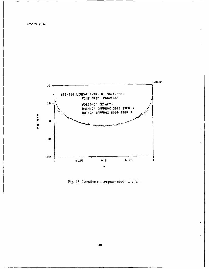
AEDC-TR-91-24
SC35241
20 -
STINT1O LINEAR EXTR. G, SA-1.0001
FINE GRID (200X100)
10- SOLID:G' (EXACT)
DASH:G' (APPROX 3000 ITER.)
G DOT:G' (APPROX 6000 ITER.)
pR 0
E
-10
0 0.25 0.5 0.75
X
Fig. 18. Iterative convergence study of g'(x).
48
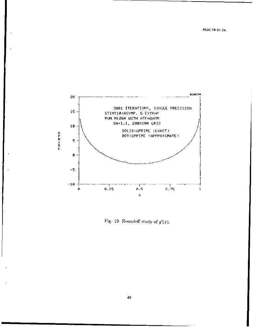
AEDC-TR-91 -24
SC352392 0 ... .... . . .... . . ..-
3001 ITERATIONS, SINGLE PRECISION15 STINT1O:ASYMP. G EXTRAP
RUN N126A WITH ATFH8Ar1M
SA-1.1, 20OX100 GRID
G. SOLID:GPRIME (EXACT)p DOT:GPRIME (APPPOXIMATE)RIm
E
-5
-10 .T- - ----o 0.25 0.5 3.75
Fig. 19. Rounidoff study of g'(x).
49

AEDC-TR-91-24
SC36240
30)01 ITERATIONS, DOUBLE PRECISION
STINTIO:ASYMP. G EXTRAPRUN N128A IITH ATFABAMM
10 SA-1.1, 200X1e0 GRID
G" SOLID:GPRIME (EXACT)p DOT:GPRIME (APPROXIMATEI
1 5m
E
-50
0 0.25 0.5 0.75
X
Fig. 20. Roundoff study of g'(x).
50

AEDC-TR-91-24
are indicated, it is speculated that the mild oscillations shown in Fig. 20 near x = 0 and 1are aggravated by the interaction of the close solid walls and the logarithmic singularitiesat these points given by Eq. (2 - 73).
2.11 Shock Fitting Scheme for Wall Interference Correction Potential
In Section 2.9, runs were discussed of the finite wall height code option associatedwith a realistic compact blended wing fighter configuration. This code has been designedto incorporate the proper source- like in-flow and cutflow boundary conditions associatedwith solid walls. In addition, d-fference 9ch2,nes were developed for the large height theoryformulated as the problem P1 in Ref. 29. The variational equation solver uses a specialprocedure to treat shock jumps in tbe solution for the wall interference correction potential€. The shock polar relating these jumps to the streamwise and transverse derivatives of 4are given as Eqs. (2 - 40) and (2 - 41).
Figure 22 shows the relationship of the geometry of a typical shock structure arisingin the 0 problem and the grid. As one choice among various options, also considered inconnection with the high aspect ratio code discussed in Section 3, the finite difference im-plementation will satisfy the shock relations across PO by surrounding it by the internalboundary condition carrying "notch" ABCD. The contour of this notch is composed oflines parallel to the F and x axes. It is presently felt that this selection provides substantialcoding simplifications as compared to another option involving a curved internal boundarynot parallel to the axes. A disadvantage of the notch scheme is that it can diffuse the shocksomewhat beyond the few mesh points necessary to capture it in the zeroth order approx-imation for the perturbation potential. However, this additional spreading is provisionallyassumed to be small, since the cases of primary concern will involve almost normal shocks.
Referring to Fig. 22, the strategy to be applied is to determine shock jumps in 4 atthe various j levels [¢] = (NSPMAX,j) - -O(NSPMIN,j) as a vector sequence
lim J,=J , (2-75)n-oo
where J, denotes the vector ([Al1, [ ]2, [ "", [)]JSMAX) at the nth successive line over-
relaxation (SLOR) sweep. The iterative sequence (2 - 75) is required since J is coupled tothe solution field €.
In the implementation, J is the solution of a bidiagonal or tridiagonal system whichis solved by recursion. The coupling of € is nonlinear through the coefficients appearingin the system. Accordingly, a linearization in pseudo-time involving the values of € at then - 1 level has been coded. The new values of J are then used for the tridiagonal systemalong x = x, lines to update the j row vectors along 4i along x = xi on the next sweep.The process is iterated until convergence is obtained.
Differencing the jump conditions (2 - 40) and (2 - 41) gives
a, [ul], + bj(ui) + c,[vi] +d1 [4b] = 0 (2 - 76a)
51

AEDC-TR-91-24
SC35237
0.6
0.4-
0.2ACp
-= _2Ag',62
0
-0.2- -
-0.41 1 1 1 00 . 0.4 0.6 1.0
x
Fig. 21. Interference pressures on a confined parabolic arc body. H 1.1, 100 x 50 grid,
1200 iterations.
52
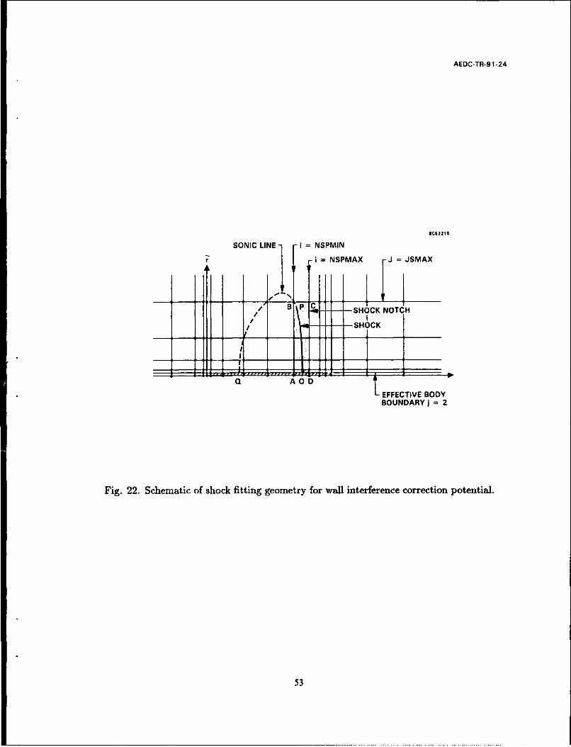
AEDC-TR-9 1-24
SCS2215
SONIC LINE - i NSPMIN
ri =NSPMAX J JSMAX
B' BPC SHOCK NOTCH __
SHOCK
Q AO oT
LFECTIVE BODYBOUNDARY] = 2
Fig. 22. Schematic of shock fitting geometry for wall interference correction potential.
53

AEOC-TR-91-24
where ( ) signifies an average across the unperturbed shock, and
a = (K -(- + 1)uo) [UO] 2 _ [va]2 (2- 76b)
b = [K - (- + 1)uol [uo]2 (2 - 76c)
cj = 2[vo] [uo (2 - 76d)
d- [v]N[°] 2[vo][vo(] - [(-( + 1)uo)uo.] [u0 ] (2 - 76e)• [ ok
Z
Using the shock iiotch idea and assuming without loss of generality, a single shock is iL theflow (fishtails for Mach numbers near unity and choking may require special treatments),denote the points in the shock notch as:
XNSPMIN, XNSPMIN+I, XNSPMIN+2, ", xNSPMAX , (2-77)
where XNSPMIN _ XHj and XNSPMAX ! XEj, and xHj, XEj denote the upstream anddownstream locations about the shock at each j, or the last hyperbolic and first ellipticpoints, re,,pectiveiy.
In more compact notation, let superscripts - and + denote the pre- and post-shocksides of the notch, respectively (NSPMIN and NSPMAX) and let s indicate the shock aswell as [€1], signify the jump of €1 at j. Then
(u +"= _ x-. - [€0].+1 -- X + OT- - - 1 (2-78)
where the i and j subscripts have been selectively suppressed.
Substitution of Eq. (2 - 78) into Eq. (2 - 76) gives the following bidiagonal system
of equations for noting that (fii) = (ui> - C, where C =
C, - B[]~
Dj 3<j<JSMAX (2-79a)
Dc =-d+ ai + b/2 (2 - 79b)A AXD
B C (2 - 79c)-Bj = j A U U
- Cj= XD AxU_ (-) (n) & () -(n
+ 2- D x o + UAO 1 + C (2 - 79d)
54

AEDC-TR-91-24
where A = j- - U signifies XNSPMIN, D signifies XNSPMAX, AXD = XD+i - XD,
AxU = xU - xU-1, n is the current time level and n - 1 the previous level.
In one version of the variational solver, central difference approximations are appliedto the discretization of the v components in (2 - 76), leading to the use of a tridiagonalThomas algorithm. The bidiagonal formulation results from one-sided differences. If therecursion proceeds downward from the top of the shock notch, it is unstable. At the top,1[ is determined from the fact that it is a body point. Section 2.16.1 provides more
information on the upward bidiagonal recursion scheme represented by (2 - 79a).
For a tridiagonal formulat;,n, there has been an issue regarding the appropriateboundary conditions at the foot of the shock, assumed located at j = 2. Since 0 (thefinite wall height perturbation potential) and Oo are logarithmically singular there, thereis a question regarding the behavior of [01]. This appears to be resolved by the fact that01,(x,U) = 0. Hence, [01,] 0 at j = 2. Moreover, in the finite wall (H) case, since
s'(x),€n If ras f -+ 0 , (2-80)
27r
then the limit F 1 0, x fixed x-, x+ , where - and + denote the upstream and downstreamsides of the shock, respectively, with S'(x) continuous at the shock gives
[] =o-oo=0 . (2-81)
Another approach is to multiply the jump equations by f and note that [4 J fr J]. Thisavoids the infinities in Eq. (2 - 81). The relation [€',] = 0 implies that
[0112 = [0113 (2-82)
Equation (2 - 82) is used to find the interference potential on the body.
A related problem was studied in Ref. 38 in regard to the invariance of the shockposition on a body of revolution in transonic flow. Some aspects of this question andconditions near the foot of the shock are discussed in the Appendix.
2.12 Determination of Second Term of Central Layer Large Height Expansion
For the numerical work, the asymptotic expansion of the velocity potential 41 in thenear field of the test article is given by (2 - 31). The constant a0 related to a' in thatexpression given by
ao - 5=(1) 1 dk (2-83)
has been numerically determined. This result gives an indication of the small H elasticity oflarge H theory, a small value being suggestive of extended validity, as in the incompressiblecase treated in Ref. 37.
55
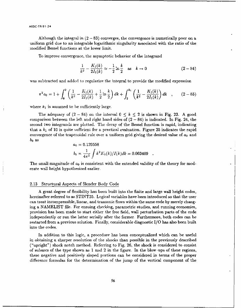
AEDC-TR-91-24
Although the integral in (2 - 83) converges, the convergence is numerically poor on auniform grid due to an integrable logarithmic singularity associated with the ratio of themodified Bessel functions at the lower limit.
To improve convergence, the asymptotic behavior of the integrand
I K,(k) 1, k-- as k--0 (2-84)k 2 21I(k) 2 2
was subtracted and added to regularize the integral to provide the modified expression
7r°= + (2(1 21,(k) +2 ) dk+ (1- K-k)- dk (2-85)
where k, is assumed to be sufficiently large.
The adequacy of (2 - 84) on the interval 0 < k < 2 is shown in Fig. 23. A goodcomparison between the left and right hand sides of (2 - 84) is indicated. In Fig. 24, thesecond two integrands are plotted. The decay of the Bessel function is rapid, indicatingthat a k1 of 10 is quite sufficient for a practical evaluation. Figure 25 indicates the rapidconvergence of the trapezoidal rule over a uniform grid giving the desired value of a0 andb0 as
a0 = 0.129558
bo _4 1 k2K,(k)/i(k)dk = 0.063409
The small magnitude of ao is consistent with the extended validity of the theory for mod-erate wall height hypothesized earlier.
2.13 Structural Aspects of Slender Body Code
A great degree of flexibility has been built into the finite and large wall height codes,hereinafter referred to as STINT25. Logical variables have been introduced so that the usercan treat incompressible, linear, and transonic flows within the same code by merely chang-ing a NAMELIST file. For ensuing checking, parametric studies, and running economies,provision has been made to start either the free field, wall perturbation parts of the codeindependently or run the latter serially after the former. Furthermore, both codes can berestarted from a previous solution. Finally, considerable diagnostic I/O has also been builtinto the codes.
In addition to this logic, a procedure has been conceptualized which can be usefulin obtaining a sharper resolution of the shocks than possible in the previously described("upright") shock notch method. Referring to Fig. 26, the shock is considered to consistof subarcs of the type shown as 1 and 2 in the figure. In the blow-ups of these regions,these negative and positively sloped portions can be considered in terms of the properdifference formulas for the determination of the jump of the vertical component of the
56

AEOC-TR-9 1-24
2.8 _
2.841 Kj K(k)
2.0 - k2 211(Wk)
___1 ____ -In-k1.6 2 2
~1.2 - T __
0.8
0.4,
0.0 7__0.0 0.2 0.4 0.6 0.8 1.0 1.2 1.4 1.6 1.8 2.0
k
Fig. 23. Comparison of exact and approximate integrands.
57

AEDC-TR-91-24
I _______.
0.-0- ___ 1L. kl (k) 1 k
- + - In-0.16 k2 21 (k) 2 2
K1 (k)
< 0.12 k2 211 (k)
0_ 1 2 3 4 5 6 71
I- I _______ I
0.0 ® I I ,
0 1 2 3 4 5 6 7 8 9 10
Fig. 24. Integrands used in evaluation of ao.
58

AEDC-TR-9 1-24
0.130
0.128 L_ __ _
0 100 200 300 400 500 600
N =NUMBER OF INTEGRATION POINTS
Fig. 25. Convergence study of a0 integration.
59

AEDC-TR-91-24
perturbation velocity [vi]. The actual relationship of the points is shown in Figs. 27a-27c which indicate a bubble over a parabolic arc body at Mach .99. The main idea isthat depending on whether range 1 and 2 is encountered, an upward/downward one sideddifference combination or the reverse is used for obtaining [vii. A tridiagonal systemfor the jump in the wall interference potential will be obtained in this scheme ratherthan the bidiagonal system associated with the shock notch method. However, this slightdisadvantage could be outweighed by thfre potential for improved accuracy.
2.14 Incompressible Validation of Interference Module RELAXV1
The large height interference (varational equation solver (RELAXV1)) code wastested to establish whether it could provide answers in agreement with the analytical onesgiven in Ref. 37 for incompressible interference pressures. As an illustration, the flow overa confined parabola of revolution ..aF considered. Here, the confining walls are solid andcylindrical. Figure 28 indicates the free field surface pressure distributions computed byan incompressible specialization of the finite height code. It is shown to indicate the stag-nation (logarithmic singularities) resolved by the SLOR method in 300 iterations. Furtherstudy is needed regarding how the numerics treat the interactions of these singularitieswith the walls.
For this case, the RELAXV1 portion of the code comparison with analytical resultsfrom Ref. 37 is shown in Fig. 29 indicating perfect agreement.
Of great interest is the convergence of both the free field (RELAX1) and RELAXVIparts of the code. During checkout, considerable study of factors influencing this per-formance aspect was made. Figure 30 illustrates one such investigation which shows theconvergence of the algorithm with number of iterations for free field pressures at differentpoints along the parabolic body of revolution in incompressible flow. It is evident that atthis speed condition, adequate convergence is achieved in about 500 iterations. A lessernumber of iterations may be needed if a "smarter" than zero initialization is used.
2.15 Transonic Application of Free Field (0th Order) Code
The numerical formulation indicated in previous sections has been applied to obtainan understanding of wall effects on slender bodies. Results will be discussed for a flow overa parabolic arc body of revolution as an illustration of the behavior of the wall interference€ field.
For the calculations to be discussed, a uniform x-grid over the body (in the interval0 < x < 1) and an exponentially stretched version off of it was employed. Exponentialstretching was also used in the direction. These variable grids are shown in Fig. 31.
Before discussion of the interference field, the structure of the free field base solutionwill be indicated. Figure 32 shows that the numerical solution tracks the analytic behavior
o, reasonably well. Considering that the mesh for this case had a large aspect ratio nearJ = 2, improvements could be obtained by configuring the grid to make the aspect ratioapproach unity.
60

AEDC-TR-91 -24
/ 61

AEDC-TR-91-~24
SC522010.4
0 0 00 00Z0:00C00Z00C00C00 0
0o o 0 00000o000000000000O0000C0~0
a0 0 CODO COo0000000000=00 0
0000000000z:0:00
0 0 000ooo~00000C000000~0~
0 c0 0 000 --------ooooooo O OO oo 000OO OZ
0 0 0 0 0000000000000000000000000
D 0 00o 000000000 000000:0z ;
0 0 0 0 0-0000000000000_
0 0 0 0 000- 00000000000 000000 000
O 0 0 0 00000000000000000000 ==-3003OO
0.0 1 1 a: I
x
Fig. 27th. Sonic bubble over a parabolic arc body at AIo,= .99, (A supersonic points, 0buI)soniC points).
0.16 SCS2202
0.12
A L
A A A A A
A A A A A A 0 -
0.0
0. A. A. 0.9A~ 0
j~~l'-., A AA A: .0 )
62

AEDC-TR-91 -24
0.205 ~ 63016

AEDC-rR-9 1 -24
SC85-341 16
3SURFACE PRESSURES
2
1P
0-
0 0.25 0.5 0.751x
Fig. 28. Logarithmic singularities associated with parabola of revolution.
64

AEDC-TR-91 -24
SCSS-341 19
01,X _VV 151Oi151
-0.01-0.020
-0.03
-0.4- EXACT, H =21' NUMERICAL, H = 2-0.5- APPROXIIH = 2
VEXACT, H = 1.4NUMERICAL, H = 1.4X
V APPROX, H = 4.
-0.10-EAT
-0.11-
0 0.1 0.2 0.3 0.4 0.5 0.6 0.7 0.8 0.9 1.0
Fig. 29. Comparison of analytical (approximate) and transonic variational code compu-tation of interference pressures in subsonic flow.
65

AEDC-TR-91-24
SCIS 34122
0.1
SYMBOL Cp (xi)
17 a 0 Cp (0)<6 0 A ,Cp (0.15)
So.. 0 Cp (0.509)
-0.1
2.3-
. 2.2-
2.1100 101 102 103 104
N = NUMBER OF ITERATIONS
Fig. 30. Convergence study of incompressible free field solution, 6 = .178.
66

AEDC-TR-91-24
------- -
x
Fig. 31. Grid used in solution.
SC38B84
40
SOLID: STINT 17I DASH: INNER SOLN
30!STINT 17, XGRID (35), PARABOLIC ARC BODY
20-
10"
0 L0 0.05 0.1 0.15 0.2
Fig. 32. .o,. behavior near the body.
67

AEDC-TR-91-24
As an illustration of the use of the code for high subsonic Mach numbers, Fig. 33shows the streamwise distribution of local Mach number at a freestream Mach numberM.o = .99 over a fore and aft symmetric parabolic arc of revolution of thickness ratiob- 0.1. In the interval 0 < x < 1, the highest curve corresponds to j = 2 and subsequentlower curves axe associated with upward j increments of 4. The dashed line denotes theposition of the sonic line and shock. The far field computational boundary for the free fieldwas at i - 5.5 in thes, calculations. It is clear from these results that the sonic line heightis approximately i - 0.2. Further results consistent with these are shown as the isoMachsin Fig. 34. A good, sharp shock formation is indicated in this figure. In Fig. 35, the shocklayer structure is indicated. This is of relevance to the use of the shock notch method.From these level lines, it is evident that the shock is almost normal. This is confirmedfrom the v0 distributions shown in Figs. 36 and 37, where it is clear that [v0] - 0. Thisleads to simplification of Eq. (2 - 40b) which is the perturbation form of Prandtl's normalsh-ck relations, i.e.,
<UO) K + *,, (2 - 86a)(2- 86b)
(uo.)
where uo is the critical value of the perturbation velocity uO. As a check,Eqs. (2 - 86) were computationally implemented and the results were close to those ob-tained from Eqs. (2 - 79). Figures 38 and 39 indicate the u0 distributions. Figure 39shows indeed that Eq. (2 - 86a) is closely satisfied by the computational solutions. Inrelated work, a hypothesis suggested by C.C. Wu concerning the invariance of the shockwave intersection with the body was analyzed in Ref. 38. Because of the structure of thenear field, this hypothesis asserts that the intersection occurs at a zero of S"(x). Numer-ical studies such as those discussed give partial but inconclusive evidence to support thisassertion*. More detailed fine grid studies are required to resolve the issue.
To appreciate the rate of decay of the solution and the subsonic nature of the farfield, Figs. 40 and 41 give three-dimensional reliefs of 0 and 0.. For pointed bodies,the forcing term of the wall interference (variational equation) is proportional to the latterquantity. The subsonic structure of the far field is consistent with the assumptions of theformulation given in Ref. 29.
2.16 Further Remarks on Difference Schemes near Shock Notch
2.16.1 Bidiagonal Approach
In connection with (2 - 40a), and flow tangency, if
[VO] =0 (2-87)
* Some aspects that relate to this are discussed in the Appendix.
68

AEDC-TR-91-24
MACH DIST. SONIC LINE SC-
r FOR SONIC LINE1.1--0.193
0.147 1
o 1.0 0.102
.056
0.00/,SHOCK NOTCH
-2 -1 0 1 2 3
Fig. 33. Streamwise distribution, parabolic arc body, M1 = 0.99.
0 .30 IC3 S843
0.994
,1.0.15 1
0.984
0.0- 09644-1.5 -0.5 0.5 1.5
Fig. 34. Formation of shock.
69

AEDC-TR-91-24
0.30 i M_ 0993 SC39432
0.15
0960
097.8 0 n
--- " 0HOCK 096 AY1063 0
0 106 ~ 09" -9
0.6 0.7J 0.8 0.9 1.0 1.1 1.2SHOCK NOTC x
YISHOCK LAYER
CRITICAL VELOCITY
Fig. 35. IoMachs showing closeup of shock.
29.3 , SC3642
r r '
v13.93
-1.56
-17.0,
-32.4 "0 0.2 0.4 0.6 08 1 0
Fig. 36. Perturbation velocity v0 over the parabolic body at M1,1 0.99.
70

AEDC-TR-9 1-24
SCIS839
10B -
-201 ,
-30-;
u SHOCK LAYER
0.6 0.7 0.8 0.9
Fi-. 37. Closeup of Fig. 36 vo distribution near shock.
71
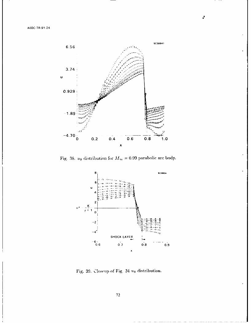
AEDC-TR-91 -24
SC3884 1
6.56
3.74 1-
o.929 .,-
-1.89~
-4.70 - -
0 0.2 0.4 0.6 0.8 1.0
x
Fig. 38. uo dlistribultion for Mf, 0.99 parabolic arc body.
8-, SC39434
U. Ky+ 1 0~
-4. i I
i SHOCK LAYER,
-6..-.0 6 0.7 0.8 0.9
x
Fig. 39. Closeup of Fig. 34 ua distribution.
72

AEDC-TR-91 -24
SC388 3 6
P)
O
x
r
Fig. 40. Three- dimensional relief of O field for Al = 0.99 parabolic arc body.
Fig. 41. Three-dimensional relief of field for M,,.. 0.99 parabolic arc body.
73

AEDC-TR-91-24
is assumed to hold beyond the weaker condition, then Prandtl's relation for normal shocksis obtained in which
(U[) = (2-88)[u0]where ( ) signifies an average across the unperturbed shock. Equation (2 - 88) can beused as a check on the numerical work.
In the bidiagonal scheme of treatinig (2 - 76a) embodied in Eqs. (2 - 79), one-sideddifferences were used to approximate the vertical perturbation velocities. This leads to therecursion relation in (2 - 79a). It is clear thal the solution of (2 - 76a) proceeds forwardfrom some initial condition associated w ih a specified j. Two options are available for thispurpose. Employing the tangency boundary conditions at the body constitutes Method 1,and utilizing the top of the shock reprcsents Method 2. Method 2 was first selected due tothe seeming inability of originally assuned Neumann data at j = 2 to provide the neededDirichlet data for the starting point. One problem with Method 2 is the possibility ofinaccuracy in prescribing the location of the tip of the shock. Method 1 can be modifiedto employ (2 - 88) instead of Neumann data at the node closest to F = 0, j = 2. This gives
2 AD + AXU (2-89)I.-] + (U0.)
A useful device in the implementation of the bidiagonal scheme (2 - 79) and (2 - 89) isthe relaxation
The quantity [v0,] 2 in (2 - 89) is obtained from the zeroth order solution.
The stability of the recursion scheme based on (2 - 79a), (2 - 88), and (2 - 89) hasbeen investigated. A tool employed is an analytic solution which has been obtained byvariation of parameters. Letting Xj = [ , this is
=_ -Ck ,(2-91)
where the products are unity when the tipper limit index is unity. A necessary conditionfor stability therefore is
Dk <1 (2-92)
We have achieved global convergence with the bidiagonal scheme with marching awayfrom the body using Method 1, providing that we use a stabilized converged free fieldsolution and a fresh start for the interference flow.
74

AEDC-TR-91-24
2.16.2 Tridiagonal Methodology
The thrust of this approach is to use second order accurate central difference approx-imations for the vertical differences rather than the first order one-sided differences of thepreviously described bidiagonal method. Employing half node points, the vertical velocityv, is given by
Vj = 1,/ = lj+ 1 / 2 + Vi,- 1 /2
201 + +1 -_ (2-93)
2
An additional benefit of this approach is consistency with the treatment of the interiornodes of the computational domain. Equation (2 - 93) leads to
10 1+ 1- [oil] [01]i_,2[vi]- [] 1~l [ll, + [ - (2-94)
-j - +j-
On the basis of (2 - 94) and (2 - 76a), it follows that
Ai(l]j+1 + Dj [,]j + B[], =C (2-95)
where
A = (2 - 96a)
2Aij+1
Di = d - -+ -AX-Daj + (2 - 96b)
-ci (2 - 96c)
-Cj = a / AxU )-___--____AXD Ax U
{,(n-l) 2(n) ^(n) 0(n)
+ 2- D+1 'U + -Uu ) +C (2 - 96d)
By (2 - 89)
A 2 =B 2 =0 (2-97a)
D2 = 1 (2 - 97b)
C2 =+ A (2 - 97c)C2= _[A1_ + (uo.)2Az7
75

AEDC-TR-91 24
At the top of the shock notch j = JSMAX, [4"] = [ 4 i],, where is
ONSPMAX - NSPMIN computing this difference as an interior point calculation. Then
DJSMA." = 1 (2 - 98a)
CJSMAY. = (2 - 98b)
Equations (2-95)-(2-98) constitute a tridiagonal system which can be A,'l,,ed by the sameThomas method employed for the interior nodes. The scheme has been computationallyiniperi'nted and its performance relative to the bidiagonal approach ib au open question.
2.17 Definitions of Interference-Free Conditions in Wind Tunnels from AsymptoticSlender Body Code
Rewriting (2 - 24a) slightly, the variational equadion foi Lhe interfei±e, c perturbationpotential 01 is
M [0i] = (Ko - (y + 1)Oo,)Oi,, + ( + (r,,,) -K1 F(x,F) (2- 99)r
with the boundary conditions
01,(X',0) = 0 (2 - 100a)
S- bR 2 P2 (cosw) + 8,rboBoRcosw +... (2 - 100b)
as R --+ oc, and the shock relations, where F = 0o, R and w are spherical coordinates, theconstants b , b0 have been defined previously and P 2 (cos w) denotes a Legendre Polynomial.In shorthand notation, Eqs. (2 - 99) and (2 - 100) can be represented as the problem P,in which
P:
M[01] = -KIF (2-99')B[0,] = G(x) (2 - 100')
where B is the boundary condition on the union of all boundaries including the free fieldshock traces. With the decomposition
01 = 0h + Op
the problems for qh and Op can be represented as
Ph:
M[Oh] =0
B[0h] = G(x)
76

AEDC-TR-91-24
M[Op] =KIF
B[0p] =0
Since M is a linear operator, qp K'I, where T is the solution of Pp with K, = 1. Thus,
O1= h + K, 4I,
Ifg, (x;K) = (Pi(x,O)
then
ADHS
so that for a specific shape, since the normalized interference drag ACD 21 "
fo' g' S'dx,
AJD - ACD K, 0) (KOI A) '(%P.xOd,X,.,C = 7(Ko, A) - I
where A = a/6 in the notation of Ref. 29 is the angle of attack parameter, and S is thenornalized cross sectional area.
With the universal relation above, the curves of ACD versus K, are linear, as schemat-
ically depicted in Fig. 42a, and can be determined once and for all for arbitrary K 1 fromthe solution of the Problen P for Ki = 1 for a given K 0 and A.
Because of the linearity with K 1 as indicated in the previous relations, the value of
K 1 = K, leading to an interference-free drag measurement can be determined explicitlyfrom the universal relation as
AG Q o(Ko, A) (2-101)f (Ko,A)
Plots of Kj* are shown schematically in Fig. 42b. Here, K represents the necessary
perturbation of the tunnel -imilarity parameter to simulate conditions leading to zerointerference drag.
2.18 Determination of Interference-Free Flows
In the preceding sections a formulation of the slender body wall interference prob-lem in which the tunnel similarity parameter is allowed to vary to achieve minimum tointerference-free flow is formulated. During the contractual effort, a computational so-
lution has been obtained representing a proof of the feasibility of this concept and also
validating the mathematical demonstrations of linearity of the interference drag ACD and
77

AEOC TR-91 24
K CDQ ;2
K1
Fig. 42a. Schemiatic of A.CD versus I.
K1
A2
A 0
Ko
Fig. 42b. Schematic of -variation of interference-free K, with Ko.
78

AEDC-TR-91-24
the tunnel similarity parameter K, given in Section 2.17. Figure 43 represents the resultof actual calculations corroborating the analysis of the previous section for the Mo, = .99flow over a parabolic arc of revolution body of thickness ratio = .1. The calculations andfigure demonstrate that interference-free drag conditions can be achieved in this case ata tunnel similarity parameter value K, = 0.14166. Additional studies concerning surfacepressure distributions can be performed in which K 1 can be optimized to achieve a min-imum, for example. in at least a mean square scise, of the interference pressure. To ourknowledge, these are the first results of this type to be obtained.
As an approximation of the numerical approach based on the bidiagonal and tridiag-onal shock jump conditions, a simplified scheme &,, been investigated. It is based on theapproximation that for slightly subsonic free stream Mach numbers the shock is normal tothe flow along its 1( _gth. This leads to the zeioth order Prandtl relations
(U1) (to(ga-,O + 40(go+.i) K (2- 102)
and Eq. (2 - 87).
For a transition occurring over zero me.sh points, the geometric interpretation of(2 - 87) is shown in Fig. 44.
2.19 Numerical Implementation
In accord with the previous formulation, a reduced interference perturbation potentialol is defined in which the far field is subtracted off. With tne notation given herein andassuming a closed body, this gives
01 = € + Cx (2 - 103a)C = 8rb0B0 1.594B0 2- 0b- 5 ;B (2 - 103b)
u, =i+C
where b0 = .063409 from nerical evaluation of the Bessel function integral (Sect. 2.1.2).
Denoting x grid points on the pre-shock side of the shock notch with s subscripts andthose on the post-shock side by p, (2 - 103) can be used to obtain a discretized form of(2 - 87) which is
I p+i ep + ._- +- C (uo.) =-gi (UO.) (2 -104)2 1Xp+ 1 xP X8 -- -I 1O
using (2 - 41b). The sum in the braces in (2 - 104) can be simplified using the definition
of [H] which leads to+ "-- + 2C
+79Zua X ) (2-105)
79

AEDC-TR-91 -24
SC471460.04 ..
0 .0 4 N Q = 0 .0
0.03 PARABOLIC BODY M =0. 990,7T= 0. 1jHXJ.AEDCJATFA8A33 AND STINT20 USED
A D0.01
0
-0.01
-0.02
-0.03 1_ _ _ _ _ _ _ _ _ _ __ _ _ _ _ _ _ _ _ _ _
-1.0 -0.5 0 0.5 1.0
K1
Fig. 43. Interference drag versus interference similarity parameter.
80
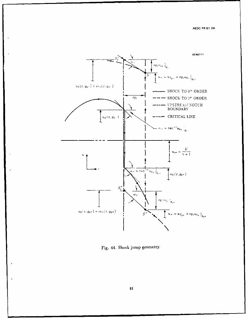
AEDC-TR-91 -24
SC48717
Y(J - ~SHOCKTO0ORESHOCK TO Is ORDER
I UPSTREAM NOTCH
t BOUNDARY
go-) CRITICAL LINE
6 tan-ito
lUcr
tan 1,
IO -T go.
Fig. 44. Shock jump geometry.
81

AEDC-TR-91-24
Equation (2 - 105) represents an explicit relationship in which points on the downstreamside of the notch can be updated in each relaxation sweep of the code. If the shock slope
is non-vanishing, [] is known only implicitly in the ridiagonal scheme of Section 2.16.2.
2.20 Results
The results to be described were computed using the bidiagonal scheme formulatedin Section 2.16.1. Others were obtained with the homogeneous Prandtl relation using theapproach outlined in the last section. These will not be shown here and give similar relativetrends but discrepancies in the actual levels. Bec.use the bidiagonal method contains the
effect of the shock shift as well as the variation of the interference vertical velocity v1 alongthe shock, it is more accurate than the homogeneous Prandtl method.
In the actual running of the solvers for the 0 th order free field basic flow and the 1 t
order interference component, convergence of both elements were monitored by studies ofthe maximum error ERRMAX over the computational domain. This error is defined asthe difference between the value of the perturbation potential at the current and previousrelaxation sweep. Figure 45a shows the behavior of this error as a function of iterationnumber for the Ot" order solution. The iteration number is a counter for the relaxationsweeps across the flow. Although the error decrease is rapid, a more reliable method ofestablishing the convergence of the solution is the drag level. This is shown in Fig. 45b.A pseudo-time asymptotic for the latter signifies stabilization of the shock location andother flow features. Convergence to the drag for the 0 th order solution usually followed the
monotonic pattern indicated with a zero initial iterate. The values of the relaxation andother parameters for such behavior will be discussed in the user's manuals. Convergenceof the 0 th order solver RELAX1 takes about 3000 iterations for the higher subsonic Machnumbers such as the .99 value of Fig. 45b. Approximately 1000 or less iterations are
required for supersonic or lower subsonic Mach numbers. Figures 46a and 46b demonstratethe convergence of the interference (variational) solver RELAXV1. In marked contrast toRELAXl, RELAXV1 is at least ten times faster. Both solvers have restart capability andthis can accelerate convergence from the performance indicated. One run strategy is to
march in Mach number space using solutions for a lower Mach number to initialize thesolution at a higher Mach number.
Both RELAX1 and RELAXV1 are scalar and unoptimized in keeping with their re-
search status. Further increases of performance can be achieved by vectorization and otheroptimizing techniques, which we anticipate will lead to seconds of run-time on CRAY ma-
chines. The order of magnitude speed increase of the 1"t order interference flow code fromthe 0 th order solver is associated with the frozen coefficients in the difference operators
during the sweeps. This is related to the linearization upon the basic flow embodied in thedescription of the perturbation interference field.
As a baseline, Fig. 47 gives pressure distributions along a parabolic arc body ofthickness ratio 6 = .1 for different Mach numbers related to the transonic similarity pa-rameter K = (1 - M) /2. Although there appears to be some upstream movement of
the shock as the Mach number is reduced from .99, this may be illusory due to the need
82

AEDC-TR-91-24
0.01 _ _ _
0.001
0.0001
0.00301 T I -- _ _ _0 500 1000 1500 2000 2500 300C
NUMBER OF ITERATIONS
Fig. 45a. ERRMAX convergence history for 01h order flow parabolic arc body 6 = .1,M = .99.
0.05
0.04 -
0.03 - /j //
0.02 1
0.01PARABOLIC ARC BODY. 5= ,1 M= .99
0 500 1000 1500 2000 2500 3000
NUMBER OF ITERATIONS
Fig. 45b. Cd convergence history for 0th order flow, parabolic arc body 6 = .1, M. = .99.
83
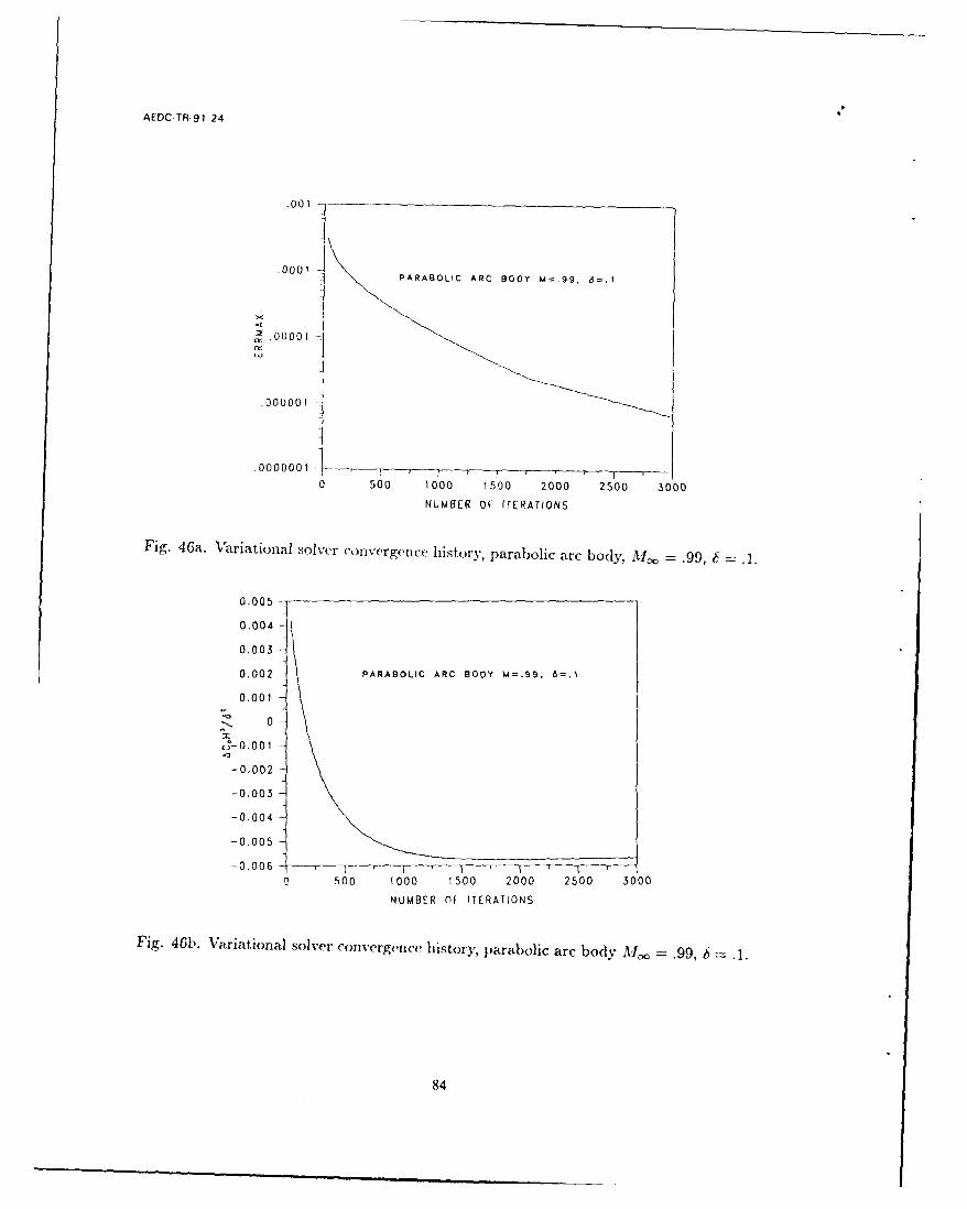
AEDCTR-9 1 -24
.001 -
0 PARABOLIC ARC BODY ,=.99, 6=.I
S.00001
.000001
.0 0 0 0 0 0 1 - -- -- -- , - -- - -- -- , - -
0 500 1000 1500 2000 2500 3000
NUMBER OF ITERATIONS
Fig. 46a. Variational solver convergence history, parabolic arc body, M0, .99, 6 .
0.005 -
0.004
0,003
0.002 PARABOLIC ARC BODY M=-99. 6=.1
0.001
J0. 0 0 1
-0,002
-0.003
-0,004
-0.005
- 0 .0 0 6 -
o 500 1000 1500 2000 2500 3000
NUMBER nF ITERATIONS
Fig. 46b. Variational solver convergence history, parabolic arc body AIf, .99, 6 .1.
84
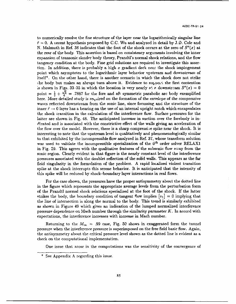
AEDC-TR-91-24
to numerically resolve the fine structure of the layer near the logarithmically singular line= 0. A tecent hypothesis proposed by C.C. Wu and analyzed in detail by J.D. Cole and
N. Malmuth in Ref. 38 indicates that the foot of the shock occurs at the zero of S"(x) atthe rear of the body. This assertion is based on consistency arguments involving the innerexpansion of transonic slender body theory, Prandtl's normal shock relations, and the flowtangency condition at the body. Fine grid solutions are required to investigate this asser-tion. In addition, there is probably a high x gradient deck neLr the shock impingementpoint which asymptotes to the logarithmic layer behavior upstream aud downstream ofitself*. On the other hand, there is another scenario in which the shock does not strike,he body but makes an abrupt turn above it. Evidence to suppo.: the first contentionis shown in Figs. 33-35 in which the location is very nearly at P dwnstrcam S"(x) = 0
point = + V3 - .7887 for the fore and aft symmetric parabolic arc body exemplifiedhere. More detailed study is required on the formation of the envelope of the compressivewaves reflected downstream from the sonic line, since focussing and the structure of theinner i -- 0 layer has a bearing on the use of an internal upright notch which encapsulatesthe shock transition in the calculation of the interference flow. Surface pressures for thelatter are shown in Fig. 48. The anticipated increase in suction over the forebody is in-(1-cated and is associated with the constrictive effect of the walls giving an acceleration ofthe flow over the model. However, there is a sharp compressi.e spike near the shock. It isinteresting to note that the upstream level is qualitatively and phenomenologically similarto that exhibited by the incompressible flow analyzed in Ref. 37, whose transform solutionwas used to validate the incompressible specialization of the 0 th order solver RELAX1
in Fig. 29. This agrees with the qualitative features of the subsonic flow a;ay from thesonic region. Clearly evident in that figure is the nearly constant level of the interference
pressures associated with the doublet reflection of the solid walls. This appears as the farfieid singularity in the formulation of the problem. A rapid localized violent transitionspike at the shock interrupts this serene behavior. It is anticipated that the intensity ofthis spike will be reduced by shock-boundary layer interactions in real flows.
For the case shown, the pressures have the proper antisymmetry about the dotted linein the figure which represents the appropriate average levels from the perturbation formof the Prandtl normal shock relations specialized at the foot of the shock. If the latterstrikes the body, the boundary condition of tangent flow implies Ivi] = 0 implying thatthe line of intersection is along the normal to the body. This trend is similarly exhibitedas shown in Figure 49 which gives an indication of the lumped normalized interferencepressure dependence on Mach number through the similarity parameter K. In accord withexpectations, the interference increases with increase in Mach number.
Returning to the Mo, = .99 case, Fig. 50 shows in exaggerated form the tunnelpressure when the interference pressure is superimposed on the free field basic flow. Again,the antisymmetry about the critical pressure level shown as the dotted line is evident as acheck on the computational implementation.
One issue that arose in the computations was the sensitivity of the convergence of
* See Appendix A regarding this issue.
85
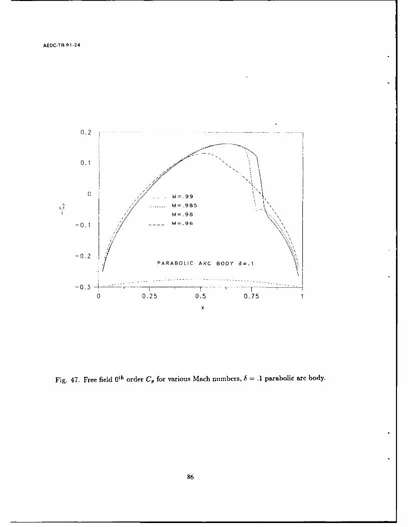
AEDC-TR-9 1-24
0.1N
-- --- - M . 8
M=.98
-0.1 ---- M=.96
-0.2PARABOLIC ARC BODY 6=. 1
-0.3-
o 0.25 0.5 0.751
x
Fig. 47. Free field 0 1h order Cp for various Mach numbers, b = .1 parabolic arc body.
86

AEDC-TR-91 -24
0.2 -
0.1
PRANDTL RELATION(g 0 ).
00
-0.1
---------------------------------------------------------- ~-------0.2 1 1 1 1
0 0.25 0.5 0.751
'C
Fig. 48. Noruiaiized interference C,, z\C,,1 3 /62 , parabolic arc body for W,,. .99, 65 =1,
(K =1.99).
87
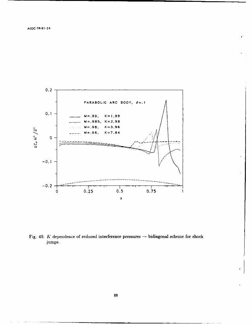
AEDC-TR-9 1-24
0.2 -_________________________
PARABOLIC ARC BODY. 6=.l
0.1 ___M=.99. K= 1.99
------ =.985, K=2.98
M=.98. K =3.9 6
00
-0.1
0 0.25 0.5 0.751
x
Fig. 49. K dependence of reduced interference pressures - bidiagonal scheme for shockjumps.
88

AEDC-TR-9 1-24
0.2 - _ _ _ _ _ _ _ _ _ _ _ _ _ _ _ _ _ _ _ _ _ _ _
0.1
-------------- ------------------
-0.3-2
0 0.25 0.5 0.75 1
x
Fig. 50. Comparison of 0 ,h order and total C,, unscaled H ]C1+, parabolic body,STINT25, M,, .99, b5 =1, bidiagonal schemne, K=I
89
AEDC-TR-91-24
interference flow to notch dimensions. This was pronounced for the bidiagonal recursion
scheme for computing [ ] at the shock but much less evident in the tridiagonal approach
described previously. Foc the calculations, the proper shock tip location and notch widthhad to be used. An approximation for the upstream and downstream legs of the notchwas obtained by a detection scheme implemented in RELAX1 in which the most upstreamand downstream location of the downstream part of the so-c line was determined. Theshock tip was defined as the subset of this locus for which the pressure gradient exceededa preassigned tolerance level. Some experimentation is required in adjusting the widthof the notch. This was accomplished most efficiently through the use in the cortrol fileLOGPARM'.RMS of indices NU, ND, JDEL which represent incremental chang-os in theupstream and downstream notch vertical boundaries at the x grid indices NSPMIN andNSPMAX respectively and the f grid index JSMAX. Some adjustment of these parameterswas necessary to prevent divergence. This inconvenience of the bidiagona! scheme overthe tridiagonal method was tolerated because it was felt that divergence was a desirablesensitive indicator of an inappropriate encapsulation of the shock. In particular, too narrowa notch allowed artificial numerical fluctuations in the 0th order shock layer to destabilizethe 1 st order interference flow. Moreover, too large or too small a value of JSMAX wasassociated with an improper location of the shock tip. In fact, for the Moc = 96 case,no shock occurs in this supercritical flow and a truly isentropic transition is obtained.Logic in the code was developed to handle this degenerate situation. At the higher Machnumbers, once a base level was obtained for convergence through proper selection of NU,ND and JDEL, rather substantial parametric elasticity was exhibited. The broad band ofthis tuning is indicated in Fig. 51 which shows that the main features of the interferencepressure distribution are retained with perturbations of these parameters. This tuning ismore delicate at the lower Moo due to the diffusion of the shock and its deviation fromnormality at its foot.
Corresponding to these pressures, Fig. 52 shows the Mach number dependence of theinterference drag. In spite of the generally increased test section Mach number due to theconstrictive effect of the walls, there appears to be an interference thrust at the highertunnel Mach numbers which increases with Mach number as the latter approaches unityfrom below. This is presumably due to the increasing net suction force on the forebody.A similar trend occurs for all the bodies tested in Ref. 36. The thrust also increases withblockage ratio, again in agreement with Ref. 29. However, before a quantitative com-parison with experiment is attempted, sting effects should be incorporated. In addition,the database of Ref. 36 is for slotted rather than solid walls. It also represents values ofH < 0.3 in contrast to the large H results given herein. The sting effect will add theadditional term to the far field given in Ref. 29.
90

AEDC-TR-91-24
0.2 - _ _ _ _ _ _ _ _ _ _ _ _ _ _ _ _ _ _ _ _ _ _ _ _1 NU=- 1 ND= I JDEL=O.AC.=-.00401 6- ------- NU=-2,ND=1 .JDEL= 0,&C.=-.005842 i'
N. 2 = - 2.N D=2.J DEL= 0ACO= -. 00567 3 1,
'01
0
-0.1
-0.2-0 0.25 0.5 0.751
x
Fig. 51. Sensitivity of interference pressures to notch size parameters, parabolic arc body,6 .1,M~ =.99, (K =1.99).
91

AEDC-TR-91-24
0.003PARABOLIC ARC BODY IN CYLINDRICAL TUNNEL
0.002
0.001
0
' 0. 001
u-0.002
-0.003
-0.004
(SOLID WALLS. M<1)
-0.005
-0.006 I i I1 2 3 4 5 6 7 8
K = (1 - M')16'
Fig. 52. Normalized interference drag ACDH'/2 as a function of transonic similarity
parameter KC (/2 9
92
AEDC-TR-91-24
3. LARGE ASPECT RATIO CONFIGURATIONS
In this section, transonic wall interference of configurations having high aspect ratiowings will be treated. The main emphasis of the theoretical and computational effort is thetreatment of wing-alone cases. There is evidence to support the belief that the wing inter-ference dominates many high aspect ratio wing-body shapes of practical importance. Inspite of this, some discussion will in fact be given to wing-body arrangements. Rather thanbeing concerned with the development of a production code, the exposition that followswill emphasize structural and mathematical features of the flow field and the descriptionof a research code that provides information on these aspects.
3.1 Theory of Far Field Boundary Conditions
A basic feature of the asymptotic theory of wind tunnel wall corrections on high as-pect ratio wings to be presented is that it systematically accounts for the influence ofthe wall modification of the far field induced downwash on the nearly two-dimensionalnear field flow over the wing. In Section 3.1.1, this coriection is obtained for free jet andsolid walls. For convenience and without great loss of generality and utility, the analysisis limited to circular test sections, although the initial setup had been made for rectan-gular test sections in Ref. 29. Section 3.1.2 generalizes the analysis of Section 3.1.1 toaccount for pressure distributions described on a cylindrical control surface. This part ofthe effort is motivated by wall interference-assessment-correction (WIAC) methods whichuse additional pressure measurements on such a control surface to account for factors notpresent in classical boundary condition simulations such as that of Section 3.1.1 and theusual perforated and slotted wall "radiation" and "oblique derivative" boundary condi-tions. The additional measurements combined with large-scale computational simulationssuch as that discussed in Ref. 39 can be used to determine if a wall correction is feasibleand evaluate it quantitatively.
3.1.1 Solid Wall and Free Jet Corrections
3.1.1.1 Discussion
An outline of the treatment of closed (solid wall) rectangular cross section test sectionsis given in Ref. 29. The treatment of pressure specified boundary condition has similaritiesto the solid wall case and important differences. For a large span wing in a tunnel ofcomparably large lateral dimensions* both the solid wall and pressure specified case havean asymptotic flow structure similar to an unconfined large aspect ratio case. The nearfield flow is essentially two dimensional at each span station (strip theory) but with anincidence field modified by downwash associated with the trailing vortex system related tothe large but finite aspect ratio. These ideas were the basis of Prandtl's lifting line theoryand have been formalized for transonic speeds as a systematic asymptotic approximationby Cook and Cole in Ref. 32. To our knowledge, no one has treated the confined case,even at incompressible speeds using matched asymptotic procedures.
* Other limits are possible such as the span tending to co at a slower rate than thetunnel's lateral dimensions.
93
AEDC-TR-91-24
Both the solid wall and pressure specified situations have nearly two-dimensional nearfields which in the asymptotic formulation reduce to the previously outlined strip theory.The finite aspect ratio downwash correction is evaluated from matching with a vortex sheetemanating from a lifting line modeling the far field (outer flow) behavior of the finite spanwing. What is different in the three cases is the nature of this downwash correction andthe structure of the far field flow. For the free field case, the near field incidence correctionis obtained from vortex and divortex representations of the lifting line. 'These can be alsoxd!ated to a doublet sheet representation as well as Biot Savart's law. For the confinedca.es, the vortex and divortex elements on the doublet sheet must be properly imaged inorder ., satisfy the wall conditions. This imaging is obviously different for the solid andp-essure specified cases and will thus produce differing incidence corrections in the near(inner flow) field.
In accord with the formulation of Ref. 29, the dominant order equation for the farfieid flow is the Prandtl-Glauert equation. This is true providing that the far field relaxesto subsonic flow, and is usually associated with high subsonic freestream Mach numbers.Slightly supersonic upstream flows which were not treated in the contract require a differentfar field treatment, involving the interaction of the characteristics or Mach waves with thecontrol surface or walls.
The Prandtl-Glauert outer flow problem can be rescaled by a stretching in the free-stream direction to give a problem mathematically equivalent to the incompressible prob-lem (Prandtl-Glauert/Goethert rules). This problem reduces to the determination of thenear field potential of a doublet sheet accounting for interactions with a control surfaceboundary on which pressures are specified. These features are shown schematically inFig. 53 for a rectangular cross section control surface Sv + SH enclosed within a rectan-gular cross section tunnel. According to the preceding discussion, pressure distributionsobtained from measurements are assumed given on the control surface. An integral rep-resentation for the perturbation potential 0 of the doublet sheet Sw can be obtained byusing Green's formula. Introducing the Green's function G corresponding to a point sourcesatisfying homogeneous Dirichlet conditions on the wall allows the wall effect to be char-acterized in terms of the control surface specified pressure distributions and removes aredundant term involving the normal velocity.
Since C. is proportional to 0x, where x is the streamwise coordinate, an integrationwith respect to x converts the problem of specifying 0. to one in which inhomogeneousDirichlet (0) data are given on the control surface.
3 1.1.2 Analysis
As has been indicated in Ref. 29, the appropriate asymptotic expansion for the velocitypotential 4 governing transonic small disturbance flow over the high aspect ratio wingshown in Fig. 54 is
- = X + 62 /3 O(X, , ; H, B, K) +... (3-1)U
94

AEDC-TR-91-24
//
/ ,, I/ SV/ I
//
----- i--4-- TUNNELI I WAL
3I BOUNDARYAND TEST
SECTION
Y FwLIFTING- |LINE
IS/ CONTROL VOLUME, \I _ _ _ _ _ _ _ _ _ _ _
Fig. 53. Lifting line in rectangular cross section wind tunnel.
where U is the freestream velocity, M. is the freestream Mach number, b is the span,
h is the tunnel dimensionless radius, 6 = wing thickness ratio, (x,y, z) are Cartesian
coordinates, r,O,x cylindrical coordinates shown in Fig. 54, b = 1/3y, = 0/3z, H =
6'/3 h, B = A.H 6"3 b, K - (1- M.) /62/3 are fixed as6 --+ 0, where A is a fixed span to
height parameter making the aspect ratio effect the same size as the wall interference. On
substitution of (3 - 1) into the exact equations, the following small disturbance equation
for the perturbation potential € results
(K- (-y+ 1)0.)0..+ + =0 ,(3-2)
or in cylindrical coordinates:
1 (3-2')
In the strained (tilde) coordinate system, the tunnel wall boundary is at f = H. Since the
pressure coefficient Cp is given by
CP = -2b'/30, (3-3)
prescribing the pressure at the wall is equivalent to specifying 4 there. In fact, measured
Cp's on the wall or some control surface can be regarded as a known left hand side of (3-3)
95

AEDC-TR-91-24
VORTEX SHEET
zx
' X
Fig. 54. High aspect ratio wing within cylindrical pressure specified control surface.
from whirh q can be obtained by an integration with respect to x from some convenientdownstream station such as -00 up tc the current x value. Anticipating the x scaling inan outer limit, the resulting Dirichlet boundary condition for 0 can be written as
O(xH,)= WQXpO) (3-4)
In accord with previous remarks, an outer expansion which gives a lifting line struct-:u, tothe high aspect ratio wing as H - oo is
p(x, p, i; H) = po(x',y',z-) - l l + 1 + "'"(3-5)
which holds in an outer limit
X .. z =- fixed asH---oo (3-6)
The transverse straining embodied in the starred variables keeps the walls fixed in thestarred coordinate system in the limit (3 - 6). The outer boundary value problem for the
96

AEDC-TR-91-24
dominant term po of the lifting line expansion is
1 1Ks,0.. + po,.... + 1 p0.. + 1(,, = 0 (3 - 7a)
p(x*, 1,0) = W(x*, 0) (3 - 7b)
Lpo]=F(z*) on the wakex* . 0,y* = 0, -A < z* < A (3-7c)
'r.here the ] signifies the jump across the vortex sheet shown in Fig. 55 and is propor-tional to the local circulation at the span station z".
i 'Y SW
Wx
/ LIFTING-' € . r - -x
t s~LIN
zF t~\-VORTEX S_
\/SEET Sc \)
Fig. 55. Far field flow configuration showing lifting line and vortex sheet.
The main result to be obtained in what follows will be the downwash at the loadedline, i.e., the value of o,. (x*, y*, z*) as x* , y* -+ 0, z* fixed.
If W(x*, 9) = 0 in (3 - 7b), then the boundary condition on the cylindrical controlsurface r* = 1 shown in Fig. 55 corresponds to a free jet. The corresponding solid wallcondition is
(*( ,1, 0) = 0 (3-8)
An integral representation for Vo can be obtained by scaling out the K factor in Eq. (3-7a)as in Refs. 30 and 32 with
) = y*/K, _ = '1K (3 - 9a)
andtan9 =/ij (3 - 9b)
2 = + 2 (3 - 9c)
97
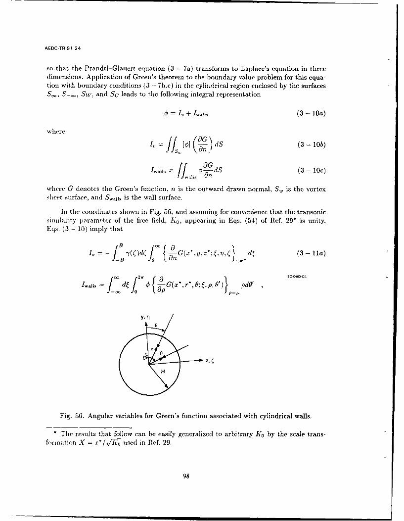
AEDC-TR-91-24
so that the Prandtl-Glauert equation (3 - 7a) transforms to Laplace's equation in threedimensions. Application of Green's theorem to the boundary value problem for this equa-tion with boundary conditions (3 - 7b,c) in the cylindrical region enclosed by the surfacesS,, S-o,, Sw, and Sc leads to the following integral representation
= lv + Iwa l.+ (3 - 10a)
where
I,= J €] ( dS (3 -10b)
Iwa,=/ 6- dS (3 - loc)
where G denotes the Green's function, n is the outward drawn normal, S,, is the vortexsheet surface, and Swan, is the wall surface.
In the coordinates shown in Fig. 56, and assuming for convenience that the transonicsimilarity parameter of the free field, Ko, appearing in Eqs. (54) of Ref. 29* is unity,Eqs. (3 - 10) imply that
I, -2 )(G(.,r*,y, *;,71,7 (idf (3 - Ila)
Iwalls _d o2, {O -G(xr 9 ; ,p, 6') odO'J70 O P=t.
Y,,
Fig. 56. Angular variables for Green's function associated with cylindrical walls.
* The results that follow can be easily generalized to arbitrary Ko by the scale trans-
formation X = x*/vPKo used in Ref. 29.
98

AFC-TR-91-24
where h = the tunnel radius in units of the root chord, b is the span in the same units,and B = 61/ 3 b, H 6 61/3 h, u = H/B = h/b. In addition, 7(() = spanwise loading= [01 = 0( ,0+, ()- 0(",0-,(), x" = x/B, y* = b113 y/B, z" = '/ 3 z/B, 6 = wingmaximum thickness, x, y, and z are the Cartesian coordinates normalized to the rootchord. In what follows, the star subscripts will be dropped.
As previously discussed, the open jet wind tunnel wall boundary condition
¢(x,/P, 0) = 0 (3--12)
corresponding to constan, pressure on the jet was assumed. For this case, G(x,p,O) ='walls = 0. The Green's f-r.rction for this problem is applicable to the generalization involvingpressure-specified boundary conditions on a control surface surrounding the test article.
The appropriate Green's function satisfying a homogeneous Dirichlet condition suchas Eq. (3 - 12) on the walls is
G - 1 os e (3-13)27np 2
E cos n-(0n- 0J) 1: )]j2
where)Ank L = Jnk
jnk are the zeros of the J,, Bessel function given by
Jn k) = 0 (3-14)and whereo(. co = 1 E
and ... -En=0 Cn('". "), where e0 1, e, = 2, n > 0.
An alternate representation for G is given by
-2--G 1 cosn(-0') cos(x - x')In( r') K.( r)- K,( H)In(Cr) d27r2 10 Jot I( H).=-oo .(n
(3- 15)Equation (3 - 15) is in a particularly advantageous form in which the free field com-
ponent can be separated out in the determination of the wall interference effect. In fact,the first term in the braces leads to the singular part of G, which is a point source in thefree field. When this is integrated from x = 0 to oo and across the span, it gives the freefield potential of a loaded line, that is, the dominant approximation of lifting line theory,which is
= j(0) 1+ _ + (z_4 r j_ 1 (2+(z )2 y + (Z-()2
This can be shown from the Addition Theorem for the modified Bessel functions
Z cosn(0 - 0')In ( r)KG(r') = Ko( R) (3 - 16a)
99

AEDC-TR-91 24
R 2 = r 2 + r'2 - 2rr' cos(O - 0') (3 - 16b)
and the cosine transform
1f 0 0 . 1Ko ( R)cos (x - x') = (3-17)4rrR 2 +(x-x') 2
Thus, the free field potential of a unit intensity isolated source is the right hand side of(3 - 17) which by Eqs. (3 - 16) is represented by the first integral in (3 - 15).
Returning to (3 - 11a). the inner integral represents the potential Oo of a line doubletparallel to the x-axis in the q = 0 plane and at the span location (. Performing the
indicated operations,
oc: aG I
1 2 ( 2 2 J, (Anr) J. (A\nk()- 2i2Cn= - n sinn k-2 Ak [Jn(Ank/L)] 2
> 0 (3- 18)
1 0 ~r)rE (2- e-AnkX) J ~k)J,(~~2riCS nsnn + 2 JL 2J.(V-J.An..=-oo An LJn(AnU)]
S< 0 -(3-19)
Of key interest is the behavior of €o and I, as x, y --+ 0. This is the essential result sought
in determining the downwash on the loaded line and matching with the inner solution. To
determine this behavior, 00 can be further decomposed as follows:
/B
00= S,-S 2 , Iv=j I (( )0d( (3-20)
where, without loss of generality, only ( > 0 will be considered*, and
01 0- 2J,(Ankr) Jn (Ak()
Y S7 n sin nO I:1- 2 ( > nsinno- - Jf(nkr) (Jn(Ank)'
2- -0 - Ak zJ (Akr tJ n(Ank) (3 -21b)
where 0 - 0 - 7r/2.
Two primary steps are employed to obtain the desired result. These are:
* Extension to ( < 0 is trivial.
100

AEDC-TR-91-24
1. Recognize that S represents a two-dimensional vortex in the Trefftz plane (and math-ematically prove it using the properties of Fourier-Bessel series).
2. Separate out the free field line doublet from S2 by using a process resembling Kum-mer's transformation to accelerate the convergence of the series. It consists of sub-tracting and adding the "tail" of the series which represents the singular part of theGreen's function associated with the free field.
Evaluation of SI
Consider the line source
G" f G(x, 0, z; , 77, ()d
then
G*(O,r,O;p,O') = - 1 cosn(O-') E J (A.kr) Jn(A7.kp)2 =.-2 Z r, 0 [0(A-kIL)] 2 (3- 22)
n= -00
G* (cc,r,O;p,0')2
From (3.13.4), p. 134 of Ref. 40, the inner sum can be evaluated as a limit of a Fourier
Bessel series. Noting that
-iZ J' )J (Jfl,) lim , (-r) {Jn-(r)Yn (P)-J. (P .("r)} (3-23)
k Ink [J. (jnk)] r-o 4 Js(,r)
and using the asymptotic properties of the Bessel functions as r -- 0, from Ref. 41, 9.17
and 9.19, Eq. (3 - 22) becomes
G*(O,r,O;p,O') = - lnp_- p-" - p-")cos n(O-0') ,n=1
0<r<p< 1 (3- 24a)
I Inr- { - - }cos n( - 0')
47r :n
O<_p<r< 1 (3- 24b)
where r _ r/pu and p - p//L. Introducing the complex variables Z = z + Zy, Z' = ( + ii7,
Eqs. (3 - 24) can be represented as a geometric series which can be summed. This gives
for It = 1,
G* (0, r, 0; r',0 ) -_ - - logZ- Z' l og Z - - -ln 0 (3-25)
101

AEDC-TR-91-24
Equations (3 - 22) and (3 - 25) demonstrate that the line source appears as a two-dimensional source reflected in the walls in the Trefftz or x = 0 plant. The first term ofEq. (3 - 25) is a free-field source at the point Z'. The second and third terms are theimage of this singularity in the walls using the inversion point 1/Z'. Equation (3 - 25)represents the classical formula for the Green's function of the first kind for a unit circle.
To evaluate S1, it can be shown that
S, G*
and therefore from Eq. (3 - 25), with Z' = on the reals,
Si- 1- /A(3-26)S 2r{(z -)2 + y + [(2) }
In accord with the previous discussion, the first term in Eq. (3 - 26) represents a two-dimensional doublet in a free field, and the second its image in the circular projection ofthe wails. The plus sign in (3 - 26) corresponds to a free jet, a negative sign is associatedwvithi solid walls.
Evaluation of S2
To implement Step 2, some preliminary processing of S2 is required. Accordingly, let
_052 1 O
2 = 2S22 1 nsinnO 1Z Okn(x,r;() (3 - 27a)5x 2ru(n=-OCI k
e-A" Jn (Ankr) J.n (nk() (3 - 27b)€}" =- Ank [J.(Ank/1) 2 ( -2 b
and
S 2 - S 2 (0)= S2 dx (3-28)
Also, letL2 (3-29)
Then, using Kummer's transformation
00 00
U=U+ Z cosn6E(-kn- 'Pk.) (3-30)n=-o k=1
I02

AEDC-TR-91-24
00 00
1: 1: P k(3-31)k=1 n=oo
Ik U e - 7ekw/ cosnOJ( Jn ( ) . (3- 32)
The %kn defined in Eq. (3 - 32) represent the asymptotic behavior of Okn in the limitk,- c+c as k --+ o. Also, the interchange of sums in Eq. (3 - 31) is assumed to belegitimate.
The quantity U is evaluated as follows: Noting from Eq. (3 - 31)
cc 00
U= E e-k' x1j >3 cos nJ,, (kr )_ (L) (3-33)k=1 -=00
from the Addition Theorem,
00 7k> cosnOJ (( = o (-R)
R = x2 + y 2 +(z - )
arid the Schldemilch series referred to in Refs. 40 and 41,+ + _[2n!]1 -B2R -P2, i , (3-34)
2-- 2 n1 }where
R=R/p-Y = nlP
B 2n = Bernoulli numberP. = Legendre polynomial
Noting that
52(0) = S ,2
and performing the integrations and differentiations of Eqs. (3 - 28) and (3 - 29), it followsthat
S2 {(Y2y + }yx (3-35)
4 7r [(z - ()2 + y2] RO(zy)00
+ x 2 Y : a11(Z - ()2(2n-~3)
n=2
103

AEDC-TR-91 24
where the O(.ry) terms arise from the second sum in Eq. (3- 30) and the term proportionalto x2 y comes froin the last sum in Eq. (3 - 34). Both of these are assumed to be negligibleregular functions conmpared to the ;ingular contributions shown. Because the singular part
has been subtracted off, tile convergence of the second sum is anticipated to be rapid. Thelast term in Eq. (3 - 35) is the dominant term of the suin in Eq. (3 - 34) evaluated by useof the expansion of P,,(v) as a finite series in v, and summing by rows instead of columns.
Discussion
From Eqs. (3 - 11), (3 - 20), (3 - 26), and (3 - 35)*, the desired expression for I,, is:
+ X
±•2( ,) 1 "CO] Y (3 -36)
4- V"Xd2 + y2 + )[(Z - +22 d ( + y
3 G
Equation (3 - 36) p)rovides the dominant inner behavior of the outer solution for theopen wall (free jet) case. It contains terms Q which correspond to the free field and Qwhich are associated with the wall effect. For a solid wall, the sign of ( is negative.
The implication of Eq. (3 - 36) on the matching of the transonic lifting line theoryof unconfined high aspect ratio wings given in Ref. 30 is that the horseshoe vortex systembecause of its imaging in the walls modifies the near field downwash by an amount asso-ciated with the term () . Structurally, the matching elements between the outer andinner solution are otherwise unchanged.
3.1.2 Pressure Specified Boundary Conditions
In the previous section, the modification of the downwash on the loaded line to freejet and solid wall boundary conditions for high aspect ratio wings was considered. In thissection, the effect of specification of arbitrary boundary conditions on a cylindrical controlsurface enclosing a high aspect ratio wing will be derived.
Referring to Eq. (3 - 7b), a decisive step in achieving this result is to split 0Po asfollow-"
Po = j + V (3 - 37)
In (3 - 37), yj is the potential associated with free jet boundary conditions, i.e.,
,,J (X, 1, O) = 0
• An alternate analysis was performed leading to the same results which used asymptotic
treatment of Fourier transform representations of the far field flow based on Tauberiantheorems.
104
AEDC-TR-91-24
The quantity ,j satisfies the jump condition (3 - 7c). Since the outer problem is linear,we can satisfy the remaining boundary condition by setting
pc(x*, 1, 9) = W(x*,9 ) (3- 38)
and [0] = 0 on the wake. Note also by linearity that pj and W, both satisfy (3 - 7a).
The problem for the correctiun potential can be solved by Fourier transforms andeigenfunction expansions. The appropriate exponential Fourier transform pair is
c - 0 eCkzc (kr*,O)dk (3 - 39a)
1 kj c-kx (*,r*,O)dx* (3- 39b)
Also, W can be represented as
W = etkiix(O, k)dk (3-40)
Accordingly, the subsidiary equation for is
1 ~ 1'.r + -r- d- 1 (wee -+k2;;=0 (3-41)
r* *
Equation (3 - 41) can be solved by eigenfunction expansions. By separation of variablesthe Sturm Liouville problems for the eigenfunctions Rn(r*) and T7'(O) are
T," -V AK2Tn = 0 (3 - 42a)
r*R" + r*Rn- (Kk 2r* 2 + ,)Rn 0 (3 42b)
The Tn and A,, can be obtained from the conditions
p(r*, 0) =(r*, -O)
'p(r*, + 27r) = )
and are T,, = cos nO, An = n = 0, 1, 2, 3,.... Equation (3 - 42b) is the modified Besselequation, whose solutions are
ln(k V-r")
The K, solutions are discarded since they violate an additional condition that Wc isbounded as r* - 0. The resulting eigenfunction expansion for ; can thus be writtenas
= AoIo(kv/-ir ) + E A,I,(kVK-r*)cosnO (3-43)n10
105
AEDC TR-91-24
Writing the transform of (3 - 7b) as
;i(1, ):W(k, 0) ,(3-44)
can be obtained as
,, _o ___- _ ) - ,,,x(k4-r*)(=(Vw(k,o )) Io(kVkr) + (k) I cosnO (3-45)
Io (kVA) l In(kVK)
where
(W(k,0)) § W(k,O)dO (3 - 46a)
W (k) = -_ W(k,O)cosnOdO (3-46b)ir
The desired results can be obtained by examining (3 - 45) in the limit y* -+ 0. Sincecos 0 = - .,this corresponds to 0 -1 Some useful asymptotic expansions in
4/y2
+z*2
V
this limit arecos(2n - 1)= (-1)"-(2n - 1) cos 0 + O(y*3 ) (3 - 47a)
cos 2nO (-1)' - + O(y* 2 ) (3 - 47b)
for n = 1,2,3,.. fixed.
Letting
Gn = Wn(k)In(kv / -'r)
I.(k /-K)
then splitting the sum into odd and even components as follows,
E( ... ) = E C, cos2nO + G ._, cos(2n - 1)0n=1 n=1
and noting that
I2n(kV-Kr" ) - I 2n(kV/k-z ) + O(y*2 )
gives
=7- ((- )n-'(2n - 1) W2n _(k) I,._,(k "z),(kO ~ n)= 1 z*n~ K=
or
Sz-1) (2n - 1) [0 ekW2nk)h"-l(kVz*)dS = 2 r- E-lcc12n-I(kV)
n=1 -o
106

AEDC-TR-91-24
so that
1 p~00 ___d
=7r Z(_- (2n - 1)]10Wnl~)..dn=1
By virtue of (3 - 46),00
W(k, o)= Wo(k) + E in(k)cos n (3 -48a)k=1
00
W(x*, ) = Wo(x" ) + 1_. Wn(x*)cosnO (3 -48b)k=1
Also,00= ]Wnj iX)~zx
Thus1 00- W00
,P,. (0, 0, z*) -(1)n'(2n - 1)1-00 W2n.(x*)dx*f1 (3 - 49)
x /0 - ikz
* I2n-l(kvrKz*)dkJ- 12n-I (kV/-K)
Here,
= W(x',O)cos(2n - 1)OdO
If it is assumed that all higher harmonics such as n = 2,3,.-. are zero in (3 - 48b), then(3 - 49) simplifies to
(00,. (0, 0, z*) L WI(x*)dx L c -ikIi(kv/z*) dk (3 - 50)27r r f (kv'rK)'
2z* 0.00 1
The inner integral in (3 - 49) can be evaluated by residues. The poles are pure imaginariesgiven by
k=ijn,s , s=1,2,3,..
where the jn, are the zeros of J, i.e.,
Jn(jn) = 0
which are all real and simple.
The higher order pole at k = 0 is negligible since the integrand is bounded at theorigin. If k = + ii7, then the asymptotic behavior of the integrand is
In "(vz ) -o( ((- 'V'-+=)) as Jk --+ o, < 0, x* > 0, jz < 1
(3 - 51)
107

AEOC-TR-91-24
which implies that the inversion integral can be evaluated by summing residues inside asemicircle (1k; = R, il < 0) in the lower half plane as shown in Fig. 57. Equation (3 - 51)insures that the integral will converge. Summing the residues gives finally after someinterchange of the orders of integration
Pc,. (0,0, s') v:1 (_1),,n J,(j,,z'),(/,),.eJ:*lx)d 3-2
000
A'ns
Fig. 57. Contour for inversion of the inner integral in Eq. (3 - 51)
where the continuation of the inversion for x* < 0 has been made. Now the integral in(3 - 49) can be expressed as
e -'Izf(x)dx 10 -- J7e jf(O) + O(A- 1 )} du
A () {f(O) +O }
if the integrand is expanded assuming that A is large. This can be a useful approximationsince j> > 3.83171. It implies finally that
f. (0, 0, Z*) - 2/ (-1.)"(n) W(J (j,,z*) (3-53)1Jl J (jnl
108

AEDC-TR-_ 24
If the higher harmonics are neglected, due to the rapidity of convergence of the series,(3 - 53) reduces to
py.(0,0,Z*) 2 W(O) J1 ( I z*) (3 - 53').0I'llKz* jj Ji )
whereW"(o) = 2 w(o, ) cos ndO7T
Thus, to obtain the wali interference associated with a series of pressure measurements ona control cylinder, only tkose at the location of the wing are important. Equations (3 - 53)give the effect of non-zero wall pressure on the downwash at the loaded line.
3.2 Numerical Procedures and Outline of Code
A formulation of the high aspect ratio problem is given in Ref. 29. As indicated inSection 3.1.1.2, the asymptotic expansioh for the velocity potential -1) is
It,- X + 6113¢(X, , ;K, A, H,B) + ...,(3-1)
which is valid in the Kerman Guderley (KG) limit
X' = /3 y, -=-3 , A = , B = l/3b, H = h 1 3 fixed as -*0,
(3 - 54)where b = thickness ratio, b = semispan in units of wing root chord, M, = Mach number,h = open jet, closed wall, pressure specified control surface radius in units of wing rootchord, and a = wing geometric angle of attack.
Within the KG limit (3 - 54), a secondary (confined lifting line) limit is considered fora high aspect ratio wing in which the wall interference is of the same order as the three-dimensional effect associated with finite aspect ratio. Accordingly, in an "inner limit" nearthe wing, the flow field is almost two dimensional with
1¢(x, ,i; A,g,p) = o(x, ;Ao,Kio,p) + - ¢(x, j,z* ;Ao,Al,i, Ko,Kl) +... (3 -55a)
K = K0 + 1K1 +"- (3 - 55b)B1
A = A0 + -A 1 +... (3- 55c)B
in the inner limitzH h
z= - X1 0, - = - fixed asB-+ oo,6--+0 independently. (3-56)
As indicated in Ref. 29, the far field for the inner problem for the finite aspect ratio,wall interference correction 01 is governed by a far field associated with an outer problemcorresponding to a bound vortex shedding a trailing vortex sheet.
In what follows, the formulation and description of the pilot lifting line code accountingfor wind tunnel wall interference will be given. The analyses will assume without excessiveloss of generality that K1 = A1 = 0.
109

AEDC TR-91-24
3.2.1 Boundary Value Problem for 00
3.2.1.1 Analytic Formulation
Input Parameters
The airfoil shape shown in Fig. 58 is given by Y,,: = 6F.,e(x), fxj _ 1,max JF = 1, i a- upper surface, f - lover surface
Angle of attack: a
Ratio of specific heats: 7 1.4
Transonic similarity parameter: bT
- 2
(or, for Krupp scaling, K - M'
Boundary Value Problem
(K - (-y + 1)0o,) 60,, + O0i = 0 (3 - 57a)
A , jx 1 (3-57b)
[€0]9=O = F for x> 1 [Kutta - Joukowski condition] (3 - 57c)
179 (7 +±1)F2In r00 170+ (-y+1r cosO+.-, asr--,oc,0<9<22r27r 167r 2 K r
(r z X2+KV) (3 -57d)
0 = tan- ')
3.2.1.2 Numerical Formulation
A rectangular computational gi id sc:ematically indicated i, Fig. 59 is employed whichis approximately uniform on and near Lhe wing, with geometric stretching in the far V.ld.(There is a capability to adapt the grid spacing on the wing to the airfoil shape, as indicatedsubsequently.) The grid is displaced from = 0 and from the singularities at (-1,0) and(1,0).
Solution values are stored in PHI(1:IMAX,1:JMAX), with an extra row/column forthe boundary values.
The airfoil ordinates are input in a table, then interpolated and differentinited (usingsmoothed cubic splines) to get the Neumann body boundary conditions. A parabolic arcairfoil and the NACA 00nn series are available analy tically.
Equation (3 - 57a) is solved by successive line overrelaxation (SLOR), based on tech-niques developed in Refs. 31, 33-35, and 42, solving the finite difference equations a lineat a time, from i=1 to i=IMAX.
110

AEDC-TR-9 1-24
SC37645
AIRFOIL GEOMETRY
L=2 1 =,&/L
F ig. 58. Airfoil geometry.
AIRFOIL
y=*-- ---- -- -- --- -- -- ------- 0 j = up
____________I_ j=fdn y dy
dx ) \ I =TRAILE
I =LEADE
Fig. 59. Complutational grid.

AEDC-TR-91-24
Basically, 3-point centered differences are used. The grid can be nonuniform. Thedifferentiation formulas employed are:
h i h2 -h, h - h, hi 2 )
00n, - 0-i,, + o, + h)o+, +O(h )
I + (h + h2 ) hIh 2 h2(hi + h2 )
2 2 24 It. , h h + h2 ) - hh 2 h2 (hi + h2 )
Set i,- K - (y + 1)0 using this central difference. Then 11ij controls the type of
the equation at (,1). There are four cases which are tabulated in Table 1:
Table 1. Type Sensitive Switches Employed by do Modules
/i-l,j 1,j Type of Point Representation of (K - (-y + 1)0,o) qo0.
(i) > 0 > 0 elliptic Pi,jo.. ,, [central differencing](ii) < 0 < 0 hyperbolic /i-iji 0.,i, [backward differencing]
(iii) > 0 < 0 parabolic 0 [y - 0 any way](iv) < 0 > 0 shock (i) + (ii)
The representations for Cases (i)-(iii) shown in the table keep the equations stableand the marching direction toward positive x. In (iv), Murman's shock point operator is
applied. This is consistent with the Rankine-Hugoniot weak solutions at the shock. For
Oo, central differences are employed, giving a tridiagonal system.
(i) In Jlx < 1, i.e., leade < i < traile, the Neumann boundary conditions are satisfied bythe following discretization method:
Above the wing, at j = fup:
S001+1 /2 - oi li-1/2 + 0 ((dy) 2 )0j+1/2 - j-/2
00 +1 -0 i
d -000=0 specified in B.C.dy
(Similarly below the wing.)
(ii) In x > 1, i.e., i > traile, there is a branch cut with constant jump I' in 00. However,Oo and Oo, are continuous across the cut. Accordingly,
at j = fup, use (€o,- + r) for Oojj_ (above cut)
at j = fdn, use (00,,+, - r) for oi+, (below cut).
Once the line i = traile(x = 1) has been solved, the circulation r is reset to [0]TE =
Otrailefup - traile,fdn and the far field is updated with this new value. The whole process
112

AEDC-TR-91-24
is repeated until Oo and F have converged. In practice, Jameson overrelaxation is used,together with cyclic acceleration.
A flow chart of the main program that computes 00 is given in Fig. 60. Descriptionsof the subroutines indicated therein follow. Additional information is given in Figs. 61-64.
Principal Subroutines
SOLVE: This calls SLOR, and manages the sweeps across the flow field including conver-gence accelerators and is depicted in Fig. 63.
SLOR: This is ttj', successive line overrelaxation module which solves for the soluticoa
column, vector on 1=constant lines (see Fig. 64).
GRID - This sets up the grid data from the user's description (see the file 2D.DOC).
Output: imax,jmax - size of grid
x(0:imax+l), y(0:jmax+1) (grid points)
dx(0:imax+l), dy(O:jmax+l) (grid spacings)
fdn,fup (lines above and below wing)
leade,traile (position of leading and trailing edges)
There is an option to adapt the grid spacing on the wing to the local slope gradientsof the airfoil. This is implemented by letting dx = b+F (z)I" Here, b is a constant which
controls the extent of the grid stretching; 2.0 is the default, while b < 2.0 will cause greatervariations in the spacing and b > 2.0 will cause less. The user can control this by modifyingthe variable "expand" in the control file. The parameter a is adjusted iteratively until thegrid just fits nicely onto the wing, i.e., x(leade) = -1 + . x(leade).
The user gets a summary of the grid and can decide if the computational domain isbig enough. (With adaptive gridding, it is difficult to tell beforehand.)
This IMSL routine fits smoothed cubic splines. ICSSCU is used with a user-specifiedsmoothing constant.
ANGLES - Calculates two arrays needed for computing the far field value of 0$ at theboundary.
angle =ta n -- t27r,
FARFLD - Updates the far field using the current value of r.
0 = r.angle + r 2.ffid2
OUTPUT - Builds two files of results, one formatted (FOR011.DAT) and one unformatted(FOR012.DAT) for graphing.
The data output are CP and Mach, the local pressure and Mach number distributions,where:
2/ =M-
113

AEDC-TR-91-24
SC37666
2DIN
READ CONTROL FILEREAD OLD DATA (.) IF AVAILABLE
(SET UP THE NEUMANN B.C.)
CALL MKFOIL Inr
ANGLES (CALCULATES u,- COS v FOR THE FAR FIELDFARFLD
SETCOF (PUT IN INITIAL FAR FIELD)(CALC. COEFFICIENTS FOR THE FINITE DIFFERENCE OPERATORS)
CALL SOLVE (SOLVE EQUATIONS TO USER'S SATISFACTION)
CALL OUTPUT (REPORT ON RUN AND WRITE GRAPH DATA)
Fig. 60. Flow chart for MAIN program computing 00.
114

AEDC-TR91 -24
SC31693
MKFOIL - BUILDS AN ARRAY CONTAINING THE NEUMANN B C VALUES F. , 4-A
CASE I FOR AN NACA 00-~ AIRFOIL OR A PARABOLIC ARC AIRFOIL THE F VALUES ARE COMPUTED ANALYTICALLY BY
SUBROUTINE FOIL
CASE 2 THE AIRFOIL HEIGHTS ARE GIVEN IN A TABLE
READ Iu 61'
COMPUTE r=MAXII ,. - MIN III
CALL ICSSCV THIS IMSL ROUTINE FITS
IOR ICSSCU: SMOOTHED CUBIC SPLINESICSSCU IS USED WITH A USER SPECIFIEDSMOOTHINGi CONSTANT
COMPUTE THE SPLINE SDERIVATIVES ON THE GRID
BUILD THE B CUI
-
Fig. 61. Flowchart of subroutine MKFOIL. C7A
(13) ANGLE (1,4)
10)
Fig. 62. Angular relations for far field.
115

AEOC rR-9 1-24
SC37674
SOLVES THE TRANSONIC EQUATION BY REPEATEDLYSOLVE CALLING SLOR UNTIL + AND r HAVE CONVERGED
TO THE USERS SATISFACTION
PRINTOUT MADE 1A01 AND F
I (THIS IS NEEDED FOR THE CYCLICIF AT ITERATION n-k j ACCELERATION
OR n-2k THROUGH A CYCLE
SAVE
IAT ITERATION n.IFAn-ESIAETELRSTIGNLUACCEERAT Al= dln-kd,,/dT nkd,,
IF NOT _ _ _ _ _ _ _ _ _ _ _ _ _ _
ACCELERATE +: + +, k +n+nk
SRECOMPUTE rU F CALL FARFLDj
Fig. 63. Flowchart for subroutine SOLVE.
116

AEDC-TR-91-24
SC37663
SUCCESSIVE LINE OVER-RELAXATIONSLOR (ONE ITERATION PERFORMED HERE)
SAVE 'PHI' IN 'OLD'J (NEEDED BY JAMESON OPERATORS)
FOR ECH CLUMNREMEMBER mi-,jIi = 1, WMAX) FOR EACH ROWCO P T(j 1, jMAX) CMUEi5 E I= K-(117+ 1) Pxi)
WHEN DONE WHEN DONED
R
TERMS FOR /K - I - ) +
BASED ON SIGNS OFpiljAND pi j
BUILD F.D. TERMS FOR
,yy
CFD INCLUDE NJUMANN BR NNO Est: )NE., 'F
RECOPUT rO YES A&il
F.D.~~~TH CUTIT IFEEC
Fig. 64. Flowchart for subroutine SLOR.
!17
|mA NOmnn um ulnnnn • nnm u nnm mmm

AEDC-TR-91-24
Mach = 1 - 62/3 M, (K - (-t + 1)€ ) (This is actually M 2 .)
Here, n and ?n are the Krupp scaling factors, as used by Krupp, n = -j; m= . For noscaling, n = m = 0.
The graph dat also contains the critical pressure,
C; =-26' -' M
7+1
above which tile flow is supersonic.
Since Cp is only known off the wing, the graphing program extrapolates linearly tufind Cpf =0±:
3 1""ly0 = Cpi .l/2di - Cpi 3/2d "
Other subroutines are shown in Figs. 63 and 64.
3.2.2 The Three-Dimensional and Wall Interference Correction €1
3.2.2.1 Analytic Formulation
Input Parameters
The relevant program modules ,reat similar and nonsimilar airfoil section wings andobtain interference corrections for these shapes. A similar planform wing is defined asone having the same airfoil section along its span but with its chord varying with span.The numerical methods employed here are a generalization of those used in Ref. 43 forunconfined similar section wings. Remarks on various geometrical aspects are:
(i) The wing is normalized by b so that it lies in [zj < 1. The half-chord c(z) is input.For an elliptic wing, shown in Fig. 65, c(z) = Vl-- z2 .
(ii) As previously indicated, the small parameter for the expansion is 1/B, where ifAR = aspect ratio,
p 6I/3 • b
= 6113AR. - , where = area of planform
AR. j c(z)dz
(iii) The wing may be in a circular wind tunnel as indicated in Fig. 66. The parameterP = is input as the reciprocal of the fraction of the tunnel spanned by the wing.
118

AEDC-TR-91-24
xz
Fig. 65. Elliptic planform.
Boundary Value Problem for 01
This is:
L [0 1 (K ( - (-I + 1) o ) , -Y + 00oo 01 + 601 0 (3 - 58a)
2. +-.asr--, (3-58b)
[¢']wakc r 1 (z) =[1]T.E. , T.E.- TRAILING EDGE (3 - 58c)
Here, d(z) and w(z) are crucial functions controlling the size of the aspect ratio and windtunnel corrections, respectively. They are given by the integrals
d(z) = I I ro _ o d 3 -5 a
(f = principal value integral)2,Z L- ro()
47r) z, +_ -2, (d (3 - 59b)
The quantity w(z) in (3-59b) has been obtained from the far field analysis of Sections 3.1.1and 3.1.2, and the (+) and (-) apply to free jet and closed wall test sections, respectively.
119
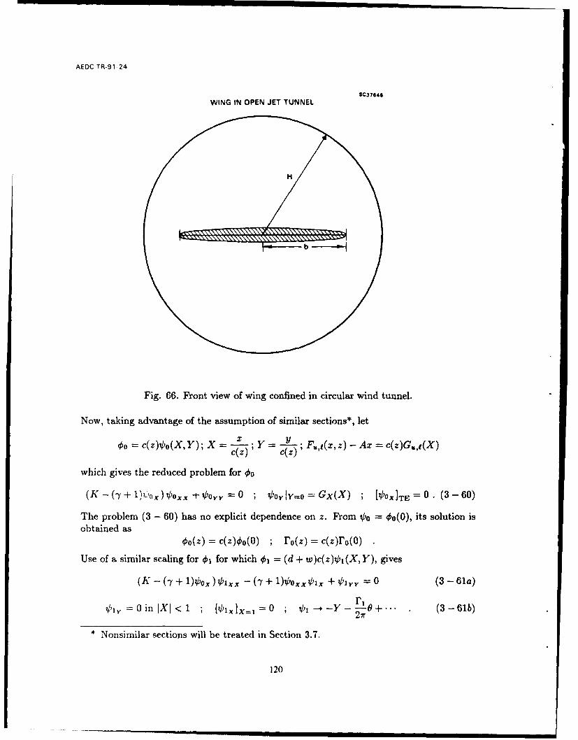
AEDC-TR-91-24
SC37648
WING IN OPEN JET TUNNEL
IH
Fig. 66. Front view of wing confined in circular wind tunnel.
Now, taking advantage of the assumption of similar sections*, let
O0=c(z)Vo(X,Y); X= Y =.Y..); F.,I(x,z)- Ax =c(z)G.,(X)c(Z) c(z)
which gives the reduced problem for 00
(K -(-y+1)',o. ) Voxx -t Oyy =0 ; Ooyly=o = Gx(X) ; [0xTE =0. (3-60)
The problem (3 - 60) has no explicit dependence on z. From tb0 = o(0), its solution isobtained as
oo(z) = c(z)4o(o) ; ro(z) = c(z)ro(0)
Use of a similar scaling for 01 for which 1 = (d + w)c(z)obi(X, Y), gives
(K - (7 + 1)Oox) 1xx - (7 + 1)0oxe,?jx + ,01, = 0 (3-61a)
V,, =O in 1X[< I ; [0l, 1x=, =0 ; 0, - -Y- r +... (3-61b)27r
* Nonsimilar sections will be treated in Section 3.7.
120

AEDC-TR-91-24
A modified form of (3 - 58) is useful to regularize the far field. For this purpose, part ofthe known far field is subtracted off and 0 = b1 + Y is solved for. The resulting boundaryvalue problem for 0* is
(K - (7 + 1)0x (0))OXx - (-y + 1)¢0xOO +€ , =0 (3 - 62a)
Ol=o 1 in Ilx < 1 (3- 62b)
F0 0 as r-4oo (3-62c)27r
[E'~]wake F -[]T.E. (3 - 62d)
The actual solution 01 is then obtained from
01(z) = (d(z) + w(z)) (c(z)* + y) (3 - 63a)
F1 (z) = (d(z) + w(z))c(z)r* (3 - 63b)
where nowd z- 0oC) 3/' c' ) . w z - ro(o)P2 1 -( d( - 63)
__4r z - < ; 47r (z;- ,2)2 w)
Within the problem given by (3 - 62), the position of the shock is known, having beencaptured by the .0 solution. It is therefore natural to fit its perturbation into the q1problem by using the shock jump relations to provide a set of internal boundary conditionsas in Section 2. These are:
[ *+ 293[O -A 100-] (3 -64a)
whereK - (- + 1)0 (3 - 64b)
= [0o]/[0o.1 (3- 64c)
andA = L [o - [€o] - 28 [Oo.,] (3 - 64d)
are known from the 00 solution.
3.2.2.2 Numerical Formulation
In the solution for 0*, all of the other scalings are applied only at the output stage.The various elements are calculated as follows:
(i) d(z)
1 I()d < r(O) c'()d6 (3-65)d 47) r 1 z- 47r z-
121
AEDC-TRf-91-24
The simplest case is for an elliptical planform, c(z) = v -z. Then,
d(z) = rc(0)/4 (3 -66)
Otherwise, the trigonometric substitution
z = -cos0 (1 -67)
is used and th', planform shape is represented by the sine series
00
c(z) =Z An sin nOn= 1
The integral 1:, - 65) thcn becomes00
d(z) r si) I EnAn sin nO (3-68)4 sin 0 n =
In practice, c(z) is given at a series of span stations. The transformation (3 - 61) is used
and a cubic spline is fitted to c(z). It is evaluated at 0 = 2r !, where m = 0,.-. n (say),
and the An are then computed with a discrete Fourier transform.
,this works well for smooth, near-elliptical planforms, but for others (e.g., sharp cor-nered wings such as rectangular and delta planforms), d(z) may have singularities whichneed further treatment.
(ii) w(z)
W2 F0(Z) dC (3-69)
Here, y > 1. Therefore, the integrand is finite everywhere, and a straightforward quadra-ture using the trapezoidal rule seems perfectly adequate.
(iii) Solution for 0* (Shock-Free Case)
In the solution of (3-62), the grid and Oo are input from some previous run which used
an identical computational grid. The coefficients (K- (-t+ 1)0o), (-j+ 1)Oo0. are computedusing central differences in elliptic regions, and backward differences in hyperbolic zones.
The parabolic value zero is used for K - (7 + 1)0o. at a subsonic to supersonic transition.This keeps the system stable. The subsonic and supersonic regions are already known from
the 0. Apart from this, the solution proceeds in the same way as for 00 .
The initial guess for 0* can be 0* = 0, an old solution, or an analytic solution to thePrandtl-Glauert equation. Since 00 and 0 -* 0 as r --* oo,
K¢ 2 + =0
122

AEDC-TR-91-24
will be a reasonable approximation, at least in the subsonic case, with the boundaryconditions (3 - 62b)-(3 - 62d). This "flat plate" problem can be solved analytically withthe following rescaling
1 . 1pxVKY)Y'=k- f = ¢+¢pyy=o , = Y 7Ko = - *F(')= (-
to give
7(x, ) =Re -iZ + i- Z2 + 2 tan-1 - +Z4 (Z (3 -70)
(Z=X + iV-K-)
To evaluate (3 - 70), the fellowing branch cuts may be used:
0<±19 ± :<27r , arg(Z+1)= _ (3-71a)
arg(Z-1)=0+ , (3-71b)
w~-erc 0+ and 0- are shown in Fig. 67. This solution has F* - which is not too farfrom the value obtained from a numerical solution of (3 - 62).
SC37638
ARGUMENTS FOR"FLAT PLATE" SOLUTION z
-1 0 1
Fig. 67. Arguments used in Eq. (3 - 70).
(iv) Treatment of Shock Conditions
From Refs. 29 and 32, the shock equations are:f[10o = 0 (3- 72a)
Zeroth order [001o= -1 12.+ oj [00. ] + [€o0]2 = o (3-72a)Z et oe _ 2 2 (3-72b)
g2 [0* ] =- g, f,32 [00'.=
First order [i-:] - l [€ ] + 20[0;] =2g{32[o..]- [po .]-213[Oo.,1} (3-73a)
t = -9 [.1-73b)
123

AEDC TR-91-24
where = K - (y + 1)00., f3 =[60 ,and x = gi(?) is the correction to the shock locus.
Eliminating g, and using the zeroth order equations yields
20[0+ =- (3- 74)
where A = 32[€,] - [Iz*] - 2,3 [4 0 j. This is the governing equation for the 0* shocks.
The shock is fitted over three mesh spacings - empirically, the numerical width of thecaptured shocks. If Pt-2,j < 0 and pi-ij > G, then the two sides of the shock notch are at(i,j) and (i - 3,j), respectively, downstream and upstream as shown in Fig. 68. The casewhen not all shock points lie between the same two grid points will be considered later.
The coefficients pj, /l-3, /3, and A are all evaluated by taking differences of thequantities evaluated at I and I - 3.
The solution proceeds normally up to and including i = I - 3. At that line, all thepoints on the notch will be either hyperbolic or parabolic. Accordingly, the differenceequations will be numerically explicit.
Lines I - 2 and I - 1 are solved normally above the notch; values for (I - 2 , jsmax)and (I - 1,jsmax) are extrapolated linearly from either side. under the assumption thatthe jump falls entirely between I - 2 aij-d I - 1. This is indicated .chematically in Fig. 69.The shock strength is assumed to vanish at jsmax.
At li-ie I, (3-74) is used to provide equations for points fup to jsmax; j = jsmax+1to jmax are treated normally as interior points in the usual manner. In (3 - 74) the jumpsare computed from
[(') : ')I ('t- (3- 75)
In the treatment of the jumps of the derivatives,
uses a two point forward difference, (dx)
0,1-3 uses a three point backward difference,e.g., 2(d.1) (30r-3 - 401- 4 + 01-5) (for a uniform grid).
€t uses a three point centered difference, -y (Oij+1 - Pij-1) (for a uniform grid)
At J = fup, the known Neumann boundary condition on the 1/2 node of tangent flowon the wing is used with the following average of point values, recognizing that the bodyis at a 1/2 node point.
0*= + + 1=0) (3-76)
Because != 1 everywhere on the wing, it cancels out in [Of]. Thus
S u (3-77)
124

AEOC-TR-91-24
tC37634
/ SHOCK NOTCH FORFITTED SHOCK
j =jsmax
I-
- - EXTRAPOLATEDfup Vjmin.I.
.J ~ - - =
1-3 -3 -2 -1 1 1
Fig. 68. Orientation of shock notch,
$C37635
EXTRAPOLATION OF 4- FOR JUMPS
€- s I "'7EXTRAPOLATED VALUES
1-4 1-3 1-2 I- 1 1 I1+ 1
Fig. 69. Linear extrapolation at shock.
This approach gives a full tridiagonal system of equations for line I. Once solved, the
solution proceeds normally at line I + 1.
The shocks captured in the 00 solution arc not always vertical. It is unlikely that the
sonic line r.-,1 stay between the same two I values for the entire shock. There seem to be
tAree options when this oc,.rs:
(i) Use a wide notch so as to cover the whole shock (see Fig. 70a). For strongly inclined
shocks (not typical of the transonic case or coarse grids), some of the information on
125
AEDC-TR-91-24
the computational grid will be iost. Also, differences (i.e., [0*]) would include more
than just the shock. This has the advantage of logical simplicity and is incorporatedin the slender body code.
(ii) Use a one point notch which follows the shock (see Fig. 70b). Here we would usedirection-sensitive differences for and stencils that look like ( or ). To get the
correct coefficients, however, ( [o etc.) they would need to be still calculated across
three mesh spacings. This could be somewhat inconsistent for some points (such asColumn I) which would be using coefficients from the middle of the nurr rical shock.
(iii) Use a three point notch which follows the shock (see Fig. 70c). This avoids ,4.ie ofthe problems of (ii), but has some of its own, e.g., how to calculate €t at points like
Q and © . Central differences (as currently used) would require 0* values from
inside the notch. These could be obtained by linear extrapolation in x, as explainedearlier, but this introduces errors of at least O(h), and possible inconsistencies.
This is the method currently implemented. Perhaps a better way to calculate Otwould be direction-sensitive one-point difference as in (ii). Here, one point forward on
the right (downstream) side and one point backward on the left for backwardly inclinedshocks and the reverse for forward inclinations.
(v) Output
The total lift L is given by
0FpU2 b [ I(z)dz , where b = semispan (3- 78)
and F(z) = total circulation
F(z) + B (d(z) + w(z))r*(z) (3- 79)
Then,
CL L Sw = area of wing = 2bL c(z)dz
M ] rdz c()f d, (3-80)1-3 c(z) d r]dz
F0/3 () f + ( + for the similar sections case(3 - 81)
M n f 1 c(z)dz
where d 41 for an elliptic planform. For the free field case,
CL=3M+ , B=61/3.AR c(z)dz (3-82)
, ,/3 . AR. for an elliptic planform.4
126

AEDC-TR-91 -24
AC3 7642
WIDE NOTCH
Fig, 70a. Wide shock votch.
SC37643
ONE POINT NOTCH
* Fig. 70b. One point shock notch.
* 0GA
THREE POINT NOTCH
Fig. 70c. Three point shock notch.I
127
AEOC-TR-91-24
Other quantities, such as the corrected pressure on the wing at a particular span station,can be similarly calculated using
1
00= +00+ (3 - 83a)
CP= -262/3€z (3 - 83b)
3.2.2.3 Program Operation and Flow Chart
Many of the modules in PHIl have the same function and implementation as in 2D. (Infact, SOLVE, ANGLES, and FARFLD are used directly by both programs.) Accordingly,only the substantial changes are discussed here.
Principal Subroutines
PHI1
Functions:
Read control file.
Read zeroth order results.
Read q*, 1* if available.
Initialize €* (method controlled by user).
(i) to 0, * = =o.
(ii) to the solution of K¢4= + ;yy = 0, by calling PHILAPL.
(iii) to an old solution.
Call WINGSC to compute the span scaling function d(z).
If y 0, call TUNLSC to compute w(z).
Call SETUP to compute partial differential coefficients, and the shock relations.
Call SOLVE to solve the 0 1 boundary value problem.
Call OUTPUT to write graphics and informative results.
Write €* and F* to OUT-FILE, if requested.
Stop.
WINGSC - Computes d(z); see Section 3.2.2.2 (i).
The wing profile is read from WING-FILE, which should consist of (z, c(z)) pairs, oneper line. This is extended, first to form a symmetrical wing, and then a periodic function,as shown in Fig. 71.
z is mapped into 0 via z - cos 0; 0 <0 < 21r. A periodic cubic spline is fitted in 0.The idea is that wings may often look like v'-- z2 near the tips; the transformation willremove the singularity in c'(z) which will help to provide a more accurate spline fit in thisneighborhood.
128

AEDC-TR-91-24
The spline is evaluated at m equally spaced points in [0,27r) where m = 2n, n =number of input and extended points. (Too many would start to fit wiggles in the splines;too few will not give enough Fourier coefficients.)
These values are used to compute a discrete Fourier transform of c(O).
The downwash integral - f '1 d (Eq (3 - 65)) is then evaluated.
These values of d(z) are then used to compute weffect = d(z)c()dz7UU)dz by trapezoidal
quadrature."weffect" is the relative lift contribution due to aspect ratio (see Section 3.2.2.2 (v)).
TUNLSC - Computes w(z); see Section 3.2.2.2 (ii).
The wind tunnel ratio p is an argument (variable urn); the integral is calculated bythe trapezoidal rule on a 51-point grid on [-1, 1].
The nteralteffct fI w()c(z)dx
The integral teffect f. (z)dz is calculated similarly to weffect. It is the relative
lift contribution due to wall interference (see Section 3.2.2.2 (v)).
SETJP - Calculates various coefficients used in the 01 boundary value problem and shockrelations (see Fig. 72).
Principal Variables
CX(1 : IMAX, 1 : 3) Computational molecule for first x derivative (centered).
CXI )= -h2 h2 - hI hi_(_'_:3) h _ (h,+_h2) h _hh h1 2)
CXX(1 : IMAX, 1: 3) Molecule for second x derivative (centered).
2 -2 2CXX(I, 1 : 3) = 2 ,
hi(h, + h2) h, h2 h2 (h, + h2)
PX(1 : JMAX, 1 : JMAX) Values of K - (-f + 1) 4o, calculated with
- central differences in elliptic regions
-- backward differences in hyperbolic regions
- parabolic (i.e., PX = 0) at the elliptic to hyperbolic transition
No shock operator is used at the hyperbolic to elliptic transition; since it is handledby the fitted shock).
PXX(1 IMAX, 1 : JMAX) Values of (-y + 1)00., using central/backward differences.
SHK(1 JMAX) Relates to the fitted shock.
129

AEDC-TR-91 24
SHK(J) = I Denotes the position of the downwind side of the shock notch at line J asindicated in Fig. 73 and = 0 if there is no shock at that line.
JSMIN, JSMAX denote the j-limits of the shock. If the shock is only above thewing say, JSMIN = FUP. If there is no shock at all, JSMAX < JSMIN.
The second part of SETUP evaluates various jumps and coefficients across the shock.and prepares them for the treatment of the numerical shock jump equation. Suppose- HK(J) = I. Then:
a [O0.] = - €0-1-3 (central differences)
ba
For this quantity, Og is calculated using central differences away from the wing. On
it, the known boundary condition, i.e., 0,, = 0 - 1 With [ _ given is employed.
c = t32 [00o] - [mio.] - 23[€0 J +- A, where p = K -(y + 1)0. = PX.
From these quantities, eight coefficients are stored in a common block for SLOR toaccess later. These are:
CJMP(J, 1: 3) = 23 . CY(J, 1 : 3) The molecule for 2f3€0,
CJMP(J,4) = A/ [, 0 -=
CJMP(J,5) =
CJMP(J, 6: 8) The computational molecule for PI-a01 ...- + A q 1 .
The differencing used here for 01, is backwards and has error 0(h2), not 0(h).
1-5 1-4 1-3
h 2 hi
The coefficients of 01-5,4,3 are:
hi -(hi + h2 ) 2h 2 + h2
h2 (h 2 ±+h2 ) hih2 h, (h, + h2 )
With these eight coefficients, the shock relation
[,U.] - [€*] +02f[€2] = -A
is represented as
CJMP01,j-1 + CJMP2 +4-sIj + CJMP30I,J+i = CJMP6 ,7 ,s " (t-5,4,3),j
- CJMP0I+I,j + CJMP,2,3 • 01-3,U
130

AEDC-TR-91 -24
SC3 7649
O-INPUT DATA FOR ,- -;O
o - EXTENDED DATA
Fig. 71. Periodic eXtension of planform.
K &C37637
k2
Fig. 72. Computationalmolecule used in SETUP. h
HYPERBOLIC ELLIPTIC
J1
1-3 1-2 I-1 1
Fig. 73. Pre and post shocksides of shock notch.
131

AEDC-TR-91-24
where U can equal J - 1, J, or J + 1.
As before, 0! at J = FDN or FUP is computed using the Neumann boundarycondition 0*1j=o = 1 (see Section 3.2.2.2 (iv)).
PHILAPL (x, g, vr-K) calculates the analytic solution to the Prandtl Glauert "flat plate"problem (PG1) KOzx + Op = 9; 0 = 1 at =0,0 < x < 1; 0 -- - as r -0 o at thepoint (x, ), with 0 = tan- ' VKP/x and r 2 x2 + K 2 .
If Z = x + iY, with 17 = 11k(j, then the solution is obtained from the incompressiblemap (IPG1) of PGI: Czz + r'y = 0 with 4 - ztan - 1 - ' as +c and
epy(x,O) = *'0< x < 1. Ihis is:
I~ +z 1=ReF(Z) - - Re 1- (see 3.2.2.2 (iii))
1 Z +_
- Re -iZ+ V1-Z2+2tan- -Z
(3 - 84)Equation (3 - 84) is obtained from integration (Ref. 44 195.04) of the complex velocityfor IPG1, F'(Z). Thus,
F'() = U - iv = i - 1(3- 85)
u=¢.(X,Y) , v= Y(X,Y)
The real and imaginary parts of (3 - 85) give
U=- r+.(sin O (3 -86a)
V = ( Cos9 (3 - 86b)
where
0±- =arg(Z:F1) , O<arg(..)<27r (3-87a)r± = mod(ZT: 1) . (3 - 87b)
Equation (3 - 84) indicates that r = -27r for the Neumann boundary conditions assumed.Equation (3 - 86a) exhibits the square root infinity in the perturbation pressure u nearthe leading edge (r- = 0), and the fulfillment of the Kutta condition [u] = 0 at the trailingedge r+ = 0. These features as well as the satisfaction of the boundary condition on Y = 0,0 < x < 1, can be ascertained from (3 - 87a).
132

AEDC-TR-91-24
In the notation of the subroutine,
arg 4 arg(Z + 1) = tan X+
arg 2 *-* arg(1 - Z) = tan-
THETA (arg1- arg2) =arg r
Quantities used to compute Re tan- ' -where tan-1 Z = I In '+'z Re(tn - 1 )(arg( z) are:
. _1_ + Z .TH ETA)a 4-* Ij:e., ae
b -- 1 Z a sin(THETA) + idcos(THETA),+b
1 -b1
a tan 4- arg(b*),
C 4- -I-z1,
THETAI +- 2(arg 1 + arg 2) (So that V/ - Z 2 = ceiTHETAI)
These results give,1
4- - {Y+c.cos(THETAI)+2.atan+r}
Figure 74 outlines the post processing operations and Fig. 75 indicates the subroutineSLOR.
3.2.3 Convergence Acceleration
Slow convergence cau r, o± '0i Lftiag cases. This is marked by the error
Ek = max 10k - ¢k-1 I
becoming small although the solution is far from its limit value.
One possible acceleration technique developed in Ref. 45 uses estimates of the largesteigenvalue(s) of the error matrix to guess the limit. If these eigenvalues are X, > X2 > •,then
€k+1 - 'kten= k + 0+
133

AEDC-TR-91-24
OUTPUT - WRITES 2 FILES OF RESULTS FORO14.DAT WHICH REPORTSON THE RUN AND FORO1 5.DAT WHICH IS UNFORMATTEDAND CONTAINS GRAPHICS DATA
COMPUTE SCALING FACTORS FOR KRUPP SCALING. n -- m =-
SCALCP -- 2d% M - n 4 3SCALM d% M FOR "NORMAL" SCALING, m = n = 0.
1 SECOND ORDER EXTRAPOLATION ISEXTRAPOLATE ,AND ON TO POSSIBLE USING SOLUTION VALUES OF
y . LINEARLY Jyly - 0 BUT IS NONUNIFORMLY VALID AT
__ "__--I LEADING AND TRAILING EDGES.
COMPUTE Cp, AND Cp1
1= SCALCP Ox)
AT y =0
LINEARLY INTERPOLATE ANOTHER POSSIBILITY IS TO PUT THE
FOR Cp1 AT THE NOTCH JUMP ALL IN ONE PLACE AS IN 2(0v)
I FOR - jsmin TO jsmax J
COMPUTE LIFT COEFFICIENTS: 1CLO-d 2/ 3 roIWFETiO T H ORDER. AND ADJUSTED FOR L0 WEFFECT+ EFCAR AND WING TUNNEL EFFECTS CL1 .CL0 (1 +
COMPUTE 0TH ORDER AND MACHO - -d23(K - ( )o,CORRECTION MACH AMACH1 - d+2 3 04 11|"
NUMBERS
4WRITE DATA TO FILES
Fig. 74. Flowchart of postprocessing elements, (repeated as Fig. 89)
134

AEDC-TR-9 1-24
SLOR - PERFORMS ONE LINE OVERRELAXATION ITERATION ON THE FIRST ORDER CORRECTION SC37670
TO THE TRANSONIC SMALL DISTURBANCE EQUATION.(K-(y + 1)+0 x1 1* 1 -Iy + 1)+,+Ox+ * =y 0
SAVE CURRENT SOLUTIONOLD - PHI
SOV TH INRIDE ONAL
fORFW NL OTCH OEASCA AFL
DGA RTE +k
Fig. 5. F OCHr fsbotn LR
135
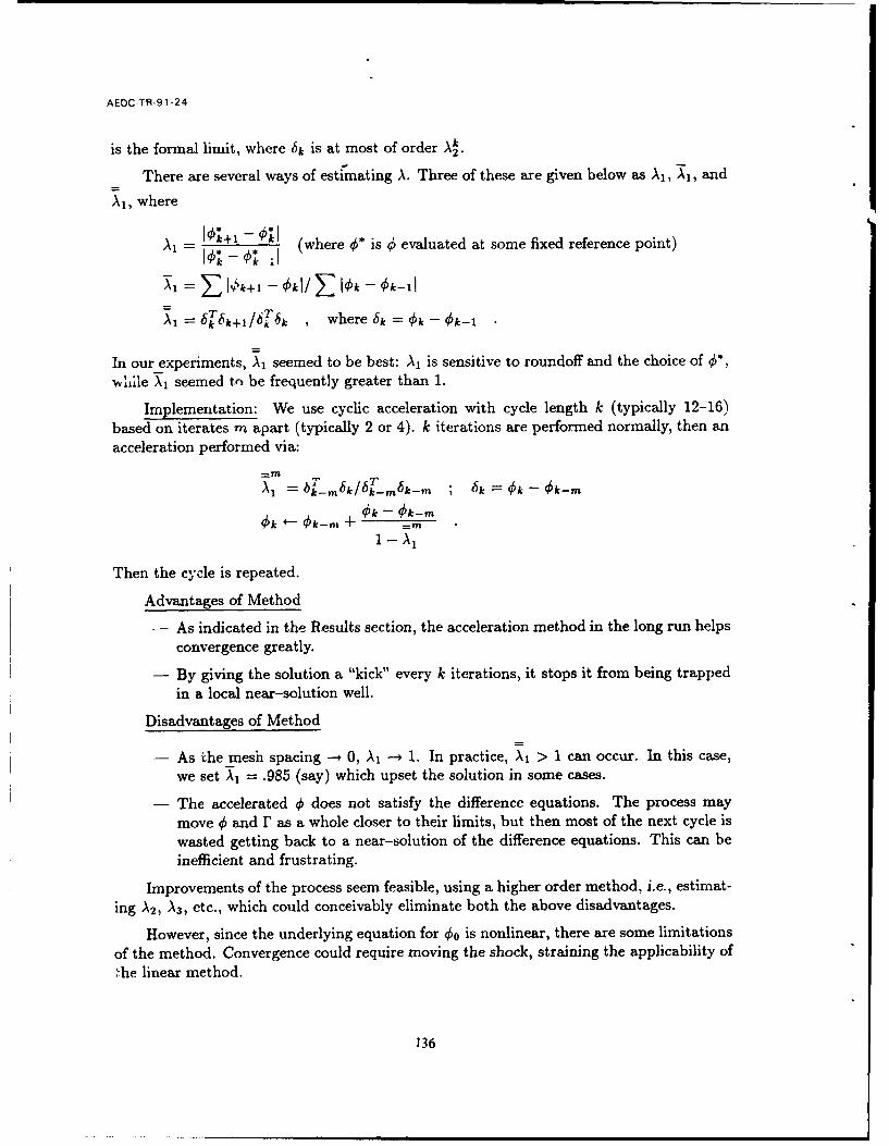
AEOC-TR-91-24
is the formal limit, where 6k is at most of order 2.
There are several ways of estimating A. Three of these are given below as A1, A1, and
A1 , where
10*+1 - '1 weA, - 0* (where * is 0 evaluated at some fixed reference point)
= I,<+, I k - O,,-,IA1 ==Z T "T I~kk4k1
1 k k+1/bk6k , where bk = Ok- €k-1
In our experiments, A1 seemed to be best: A, is sensitive to roundoff and the choice of 0*,W111ile X1 seemed tn be frequently greater than 1.
Implementation: We use cyclic acceleration with cycle length k (typically 12-16)based on iterates m apart (typically 2 or 4). k iterations are performed normally, then anacceleration performed via:
A1 = i-,. /km k-,nmk-,-T bk = Ok - Ok-,n
Ak Ak-m + -M1- A1
Then the cycle is repeated.
Advantages of Method
- As indicated in the Results section, the acceleration method in the long run helpsconvergence greatly.
- By giving the solution a "kick" every k iterations, it stops it from being trappedin a local near-solution well.
Disadvantages of Method
- As the mesh spacing --+ 0, A1 -* 1. In practice, A1 > 1 can occur. In this case,we set \1 = .985 (say) which upset the solution in some cases.
- The accelerated ' does not satisfy the difference equations. The process maymove € and F as a whole closer to their limits, but then most of the next cycle iswasted getting back to a near-solution of the difference equations. This can beinefficient and frustrating.
Improvements of the process seem feasible, using a higher order method, i.e., estimat-ing A2, \ 3, etc., which could conceivably eliminate both the above disadvantages.
However, since the underlying equation for 00 is nonlinear, there are some limitationsof the method. Convergence could require moving the shock, straining the applicability of,.he linear method.
136

AEOC-TR-91-24
3.3 Results for Subcritical Interference Flows
Figure 76 indicates the power of the convergence acceleration method for calculationof a supercritical Mo, = .75, a = 20 flow over a NACA 0012 airfoil on a relatively fine grid.Without acceleration, the circulation has not converged at 500 iterations. By contrast, theacceleration method provides impulsive corrections to achieve almost the asymptotic valueof the circulation within the same number of sweeps. The relaxation parameter w was setequal to 1.7 for these calculations.
Computational studies of the wall interference effect were made on similar sectionwings. Figure 77 indicates chordwise pressure distributions associated with the dominanttwo-dimensional term 00 at Mo, = .63 and a -= 20 (solid curve) for a NACA 0012 airfoilwing. This variation has the characteristic leading edge singularity. At higher Mach num-bers, clustering the grid ncar the leading edge was important in achieving convergence.The relative corrections associated with finite aspect ratio and wall interference (01) arealso shown for the same set of flight conditions for an aspect ratio (AR) = 8 elliptic plan-form. The dotted curves indicate the free field finite aspect ratio chordwise distributionson upper and lower surfaces and the dashed lines denote the additional wall interferenceeffect for a circular open jet test section using the far field correction worked out in Sec-tion 3.1, given as Eq. (3 - 59b) herein. In the figure, C* denotes the critical pressure level.A mean value Cpm... is shown for Cp in which
E c(z)CpdzcP,.... = y:, z
The parameter p is the reciprocal of the semispan in units of the tunnel radius.
Accordingly, the case indicated in Fig. 77 corresponds to a semispan of 95% of the tunneltest section radius. In agreement with the assumptions of the asymptotic method, thewall interference correction for this case is numerically of the same order as the free fieldthree-dimensional correction associated with finite aspect ratio and the induced angle ofattack correction of the trailing vortex system. The correction appears to peak near theleading edge and is greater on the upper surface of the wing than the lower at this positiveincidence.
The associated isoMachs for this case are shown in Figs. 78-80. Figure 78 indicatesthese lines for the zeroth order two-dimensional solution. Figure 79 shows those corre-sponding to the incremental effect of aspect ratio and wall interference associated with €1.The resultant field is shown in Fig. 80. In Fig. 79, it is interesting to note the persistenceof the leading edge singularity of the 00 field in the isoMach pattern.
For the elliptic planform of Fig. 77 at Mc, = .63, and a = 20, Fig. 81 shows thevariation of the chordwise pressure distribution along the span due to the combined effects
of wind tunnel wall interference and finite aspect ratio. Analytical evaluation of (3 - 59b)specialized to the case of the elliptic planform fully spanning the tunnel (p = 1) indicatesthat there is a square root infinity in the span load distribution at the blocked wing tipsat their intersection with the open jet or solid wind tunnel walls. This trend persists for
137

AEDC-TS-91 -24
SC37662
1.6 -
1.5
1.4
1.3
F
1.2 - NACLRTO
1.1
1.0-
0 100 200 300 400 500N =NUMBER OF ITERATIONS
Fig. 76. Effect of convergence acceleration on attainment of asymptotic value of circu-lation r.
138
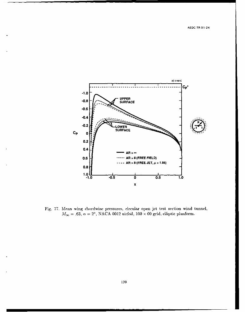
AEDC-TR-9 1-24
SC-0180-E
------------------ ---------- ---------- ----------- Cp*
-1.0
L0.WERPPER
-0.46 Ro
-0.4 R= FREFED.~A 8 ... R.E....,...1.05)
0.4
AI~~~~~~~-- .63 = 80 (FAEA 002aroi,10T 0g, elipicp0nfr)
0.'39
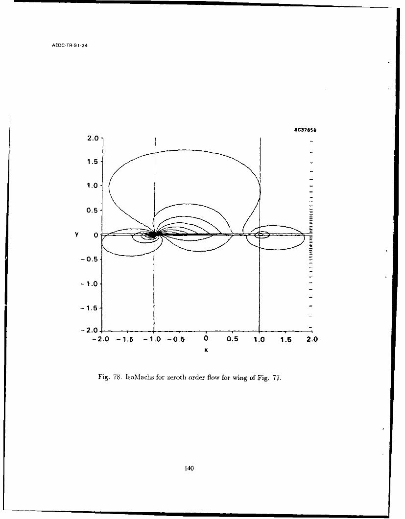
AEOC-TR-91 -24
SC37658
1.5-
1.0-
0.5-
-0.5-
21.01
-2.0 -1.5 -1.0 -0.5 0 0.5 1.0 1.5 2.0x
Fig. 78. IsoMachs for zeroth order flow for wing of Fig. 7-7.
140

AEDC-TR-9 1-24
2.01
0.5-
V 0
-0.5-
-1.0-
-1.5-
-2.0-2.0 -1.5 -1.0 -0.5 0 0.5 1.0 1.5 2.0
x
Fig. 79. Perturbation (001 isoMachs for wing of Fig. 77.
141

AEDC-TR-91-24
SC376592.0
1.5-
1.0-
0.5-
Y 0-
-1.0-
-1.5-
-2.01- 2.0 -1.5 -1.0 - 0.5 0 0.5 1.0 1.5 2.0
x
Fig. 80. Total (0+ IOisoMaclis for wing of Fig. 77.
142

AEDC-TR-91-24
the # = 1.05 case, since the wing almost spans the tunnel. Accordingly, the chordwisepressures are almost identical ai stations over most of the span, but change drastically atthe tips as shown in Fig. 81. Studies of this type for the supercritical case could guide thetwist of the wing to achieve effective free field conditions in the tunnel.
Associated with these pressures are the spanwise load distributions shown in Fig. 82.The ordinate is the sectional lift coefficient along the span normalized to the two-dimensional value for M, = .63 and a = 2. Also shown is CL/CL0 , the total winglift coefficient cor:esponding to the separate and combined effects of finite aspect ratio andwall interference normalized to the two-dimensional value. Here, the forementioned exag-gerated tip effect is evident and is connected to the wall interference. For this 95% spanningof the test section, both effects combine to give a reduction of the two-dimensional liftby 42%.
The effect ,f planform shape on these sectional lift distributions is shown -11 Fi6 . 83,where the chord variation 4
c(z) = (I -
is considered at the same conditions as the elliptic one of Fig. 77. In contrast to theconstant downwash effect of the trailing vortex system for the elliptic planform, the freefield finite aspect ratio correction now also shows a variable twist effect along the span.For the elliptic wing, this was associated only with the wall interference. It is interesting tonote that in spite of this, the magnitude of the total lift reduction due to combined finiteaspect ratio and wall interference is still approximately the same as that for the ellipticplanform.
Supercritical shock capturing will be described in what follows. Of interest in con-nection with the shock fitting required for the 01 solution is the "crispness" of the shockscaptured by the qo solution. Figures 84 and 85 show pressure distributions along variouslines j = 1,2, 3,---, jMAX for coarse and fine grids, respectively. Figure 85 indicates thatour algorithm captures the shock over 2 to 3 mesh points. In Fig. 86, the relationship ofthe jumps to the Rankine Hugoniot shock polar is shown. If ul and v, represent preshockreference states, the abscissa and ordinate used for the figure are respectively
- b + -1)(u-ui)(- + 1)ul - K
-Y ( +1)(V - V) { 3 3/ 2
4 (7+1)ut - K I
where u = qo, v = Oo, and K is the transonic similarity parameter defined previously.The various curves progressing from the U axis upwards each represent the variation of Uwith :U along g = constant lines, starting with a level closest to the airfoil and movingupwards in unit increments of j. The sharp break in the curves near the non-diffused partof the shock occurs at its downstream side. The proximity of the kink location to the polaris a validation of our algorithm to capture the proper Rankine Hugoniot jumps.
As indication of the effectiveness of the grid clustering employed, Fig. 87 shows iso-Machs for the more supercritical NACA 0012 flow corresponding to M. = .8 and a = 20.
143

AEDC-TR-91 -24
SC- 1357-T4 -- -- -- -- -- C P
-1.0 z 0 .
-0.44
-0.6 .
z0.8
.0 AR I
-1. =-0.5 0 0.5 1.0NUNE
Fig. 77 = .6, a 0.8 = .5
0144
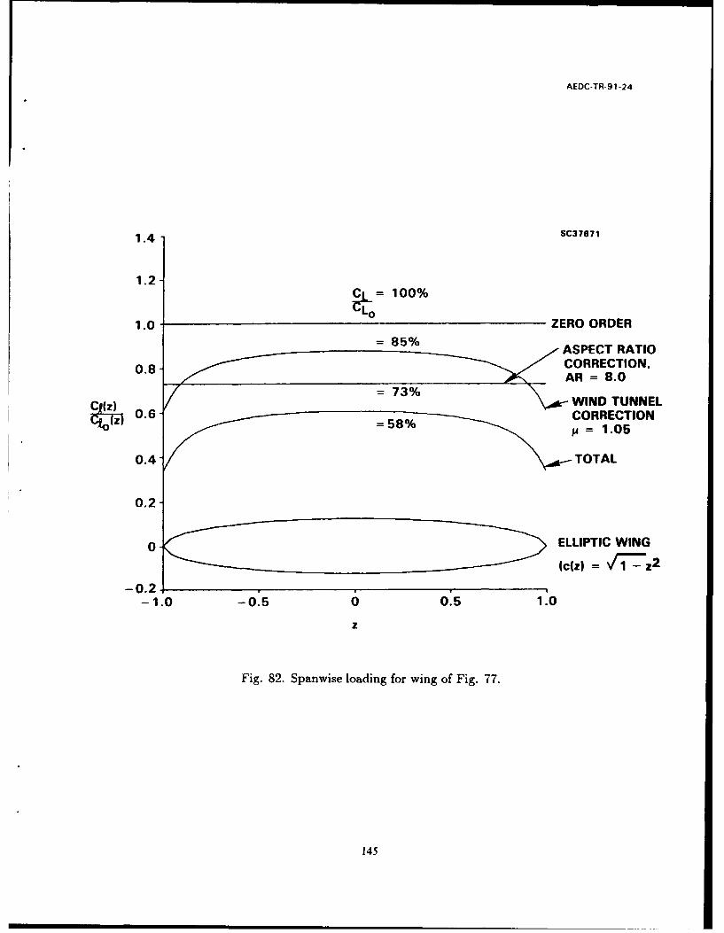
AEDC-TR-9 1-24
1.4 -SC37671
1.2-C=100%
1.0- ZERO ORDER= 85%ASPECT RATIO
0.8- CORRECTION,
0.Z)6 -CORRECTION
0.4- TOTAL
0.2-
0 ELITCWN
- 0.2-1.0 -0.5 0 0.5 1.0
z
Fig. 82. Spanwise loading for wing of Fig. 77.
145

AEDC-TR-91-*24
1.4 8C37453
L,= 2-D VALUE FOR WING
1.2 C 10%C =2-D VALUE FOR SECTION
a CL01.0- ZERO ORDER
87% ASPECT RATIO CORRECTION.
_j WIND TUNNEL CORRECTION.
72
N_j NON-ELLIPTIC PLANFORM
0
-0.2 ELLIPTIC PLANFORM
-0500. .
z
Fig. 83. Spanwise loading for nonelliptic wing. All other parameters identical to thoseassociated with Fig. 77.
146
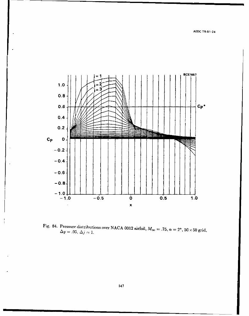
AEDC-TR-9 1-24
0. SC37657
0.2-
-0.2- p
-0.4-
-0.6-
-0.8-
-1.0,- - ~ - --------
-1.0 -0.5 0 5 1.0
x
Fig. 84. Pressure distributions over NACA 0012 airfoil, M . .75, a = 20, 50 x 50 grid,A=.05, ilj
147

AEDC-TR-91 -24
1.2 SC37654
0.8 LAST CRITICAL Cp =>TOP OF SHOCK
0.4-
-Cp
- 0.4-
-0.8-
I -30 32 54 3 440424444 C0 62 t 402440M4572 74 71
-1.0 -0.5 0 0.5 1.0x
Fig. 85. Pressure distributions over NACA 0012 airfoil, M,, = .75, a=20, 98 x 60 grid.
148

AEDC-TR-9 1-24
lIC37692
1.0-
0.5-
0-2.5 -2.0 -1.5 -1.0 -0.5 0
Fig. 86. Variation of perturbation downwash with pressure in relation to shock hodo-graph, M,, = .75, a =2*, NACA 0012 airfoil.
149

AEOC-TR-91-24
Formation of the recompression shock on the rear of the airfoil is evident in these patterns.The horizontal and vertical grid clustering employed are shown near the frame of this plot.
3.4 Supercritical Interference Flows
In Fig. 88, a result is shown for a supercritical interference flow. This calculationrepresents the chordwise pressures over an aspect ratio 8 elliptic planform which spans90% of a circular wind tunnel. The wing is at 20 angle of attack, at a tunnel Mach numberof 0.7, and has similar NACA 0012 airfoil sections along its span. The effect of the openjet and aspect ratio is to weaken the shock as anticipated.
In the treatment of these supercritical flows, the numerical methods were refined sothat the shock fitting methods can adequately handle stronger supercritical cases associatedwith Fig. 88. Two issues dealt with in this connection are the 40' shock fitting proceduresand the treatment of the surface boundary conditions.
In connection with the shock issue, it is useful to note that in practically interestingcases, the shock is almost vertical and the region about it can be contained with a verticallyoriented boundary ABCD as shown in Fig. 68. The zone inside the "shock notch" ABCDis a "hole" for which it is not necessary to compute the interference potential 4*. On theother hand, a staggered boundary of a mesh width of three points shown in Fig. 70c canalso be used to satisfy the appropriate jump conditions across the shock. The configurationof Fig. 68 is advantageous from the standpoint of programming logic, particularly in thetreatment of jumps in 0;((0; ) so that differentiation inside the notch is avoided. Thedisadvantage is that the shock region may be unnecessarily widened. However, for nearlyvertical shocks associated with Mach numbers close to unity and fine grids, this disadvan-tage can be offset. The three point staggered notch has the advantage of following theshock contours.
Subroutines SETUP and SLOR have been optimized so that numerical treatment ofthe staggered and upright notch can be built into these modules. SETUP is a subroutinethat calculates the coefficients needed in the variational (1st order) equation from thezeroth order basic flow solution. It is used in subroutine SLOR and also detects the shockas well as finding the coefficients for the 1"t order jumps. SLOR is depicted in Fig. 75.
Other capabilities that are included in the code are adjustment of notch width andbatch capability. In regard to the former, the adjustment can be made asymmetrically inthe streamwise direction to model the shock layer adequately.
In regard to the boundary conditions, boundary points are handled by averaging theslope information on the boundary with that at the immediately adjacent vertical nodepoint. The resulting discretization is given as Eq. (3 - 76) which is used to numericallyevaluate the terms in the equations of motion. Referring to Fig. 59, additional accuracyand consistency with the locally second order accurate discretization for interior points canbe achieved based on a Taylor series method. These use the first three vertical nodes pointsshown in the aforementioned figure. In the upper half plane, noting these by indices 1, 2,
150

AEDC-TR-9 1-24
3.0- SC37665
1.0-
y 0.
-1.0
-2.0-
-3.0.-5.0 -3.0 -1.0 1.0 3.0 5.0
x
Fig. 87. IsoMachs for NACA 0012 airfoil, M. .8, a 20, grid adapted to leading
edge bluntness.
151
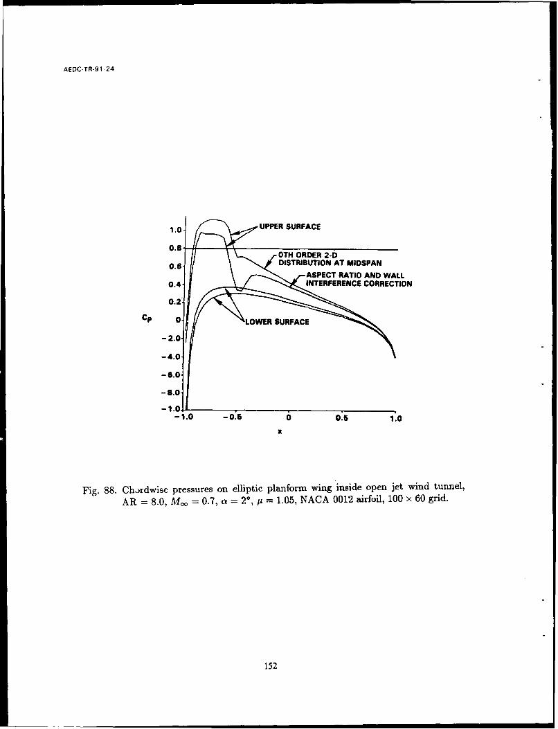
AEDC-TR-9 1-24
ASPECT RATIO AND WALL0.4- INTERFERENCE CORRECTION
0.152

AEDC-TR-91-24
and 3 corresponding to fup, fup + 1, and fup + 2 and letting
hi = Y2 - YI
h2 = Y3 - Y2
it is possible to obtain a locally second order accurate expression for 0. at Y2 in terms ofOy at y = 0, which is not a node point. The Taylor series gives simultaneous equationswith information which allows 0 at y = 0 to be eliminated so that the following expressioncan be obtained:
2h 3 - 2hih - h 3 hi(3hi + h2 ) h2
hih 2 (hi + h2 ) (2h 2 + h2) h2 (h1 + h2) (2h, + h2) 2h, + h2€' Iv=0,
(3 - 88)
where Oy I =0 is specified in the boundary conditions.
With the PHI1 code modules charted in Figs. 75 and 89 and other figures, anM,, = 0.75, a = 2* case was computed for an elliptic planform, aspect ratio 8 wing.The wing was assumed confined by a circular cross section free jet wind tunnel, with thewing spanning 95% of the tunnel diameter.
To accelerate the convergence of the iterative scheme, the special method described inSection 3.2.3 involving the eigenvalues of the error matrices was used. This is particularlyimportant for transonic lifting cases involving supersonic bubbles whose dimensions are asubstantial fraction of the airfoil chord such as this one considered here. In Fig. 90, theconvergence history of the tunnel wall perturbation of the circulation is shown. Rapidconvergence is achieved after only 200 iterations for this grid which had 50 points on theairfoil and '0 vertical nodes. An important factor controlling this behavior was the propertreatment of the shock notch. Referring to Eqs. (3 - 73), particularly, the factors [0..],[00" ]? [40o.], and [Oo,], it is imperative in this stronger supercritical case that no differen-tiation is performed inside the rapidly varying and possibly numerically dispersive shocklayer which computationally models its physically discontinuous counterpart. In addition,the width of the notch should be adjusted so that the full Rankine Hugoniot transitionis achieved. This is based on the weak solutions associated with the divergence form ofthe small disturbance equation. As discussed in Section 2.20, the streamwise pressurevariations at various heights above the airfoil depicted in Fig. 85 and the isoMachs -hownin Figs. 91 and 92 have been considered in establishing the upstream and downstreamboundaries for the shock notch.
The basic wind tunnel wall effect of this NACA 0012 similar wing gives rise to correctedisoMach patterns shown in Fig. 93. Clearly evident in this figure is the shock notch.
3.4.1 Refinements of Shock Fitting Procedures
As indicated in Ref. 29 and Section 3.2.2.2 in the numerical implementation of tran-sonic lifting line theory for wind tunnel wall interference, the shock is captured for the 0thorder approximation to the flow, while the 1 t order perturbation is fitted.
153

AEDC-TR-91-24
OUTPUT - WRITES 2 FILES OF RESULTS FORO14.DAT WHICH REPORTSON THE RUN AND FORO I6.DAT WHICH IS UNFORMATTEDAND CONTAINS GRAPHICS DATA
COMPUTE SCALING FACTORS FOR KRUPP SCALING, n,-3 m = 4
SCALCP = -2d% M -4 3SCALM = d% Mm FOR "NORMAL" SCALING, m - n - 0.
-7 SECOND ORDER EXTRAPOLATION ISjEXTRAPOLATE LiAND *ON TO POSSIBLE USING SOLUTION VALUES OFA -0 BUT IS NONUNIFORMLY VALID AT
________________ LSADING AND TRAILING EDGES.
COMPUTE CP0 AND Cp1 11= SCALCP 0,)
AT y = 0
I LINEARLY INTERPOLATE I ANOTHER POSSIBILITY IS TO PUT THEFOR Cp1 AT THE NOTCH JUMP ALL IN ONE PLACE AS IN 2(iv)
I FOR j = ismin TO jsmax
GET gl(j) = - WUSFO'0 FE
0 TH ORDER, AND ADJUSTED FOR ___-____1________+ EFFCTr*AR AND WING TUNNEL EFFECTS CL1 -C
COMPUTE 0 TH ORDER AND MACHO - -2/3 (K - (y + 1)+OCORRECTION MACH AMACH1 62/3 (y + 1)+
NUMBERS x
WRITE DATA TO FILES
Fig. 89. Flow chart of OIJTPUT module relevant to variational solver for interference
potential, repeated version of Fig. 74 for convenience.
154
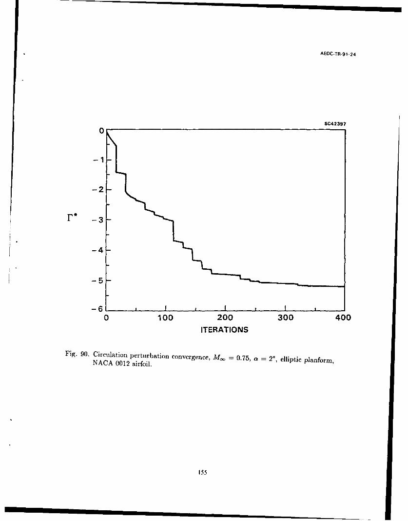
AEDC-TR-9 1-24
SC-42397
0
-2-
-3
-4-
-61 1 10 100 200 300 400
ITERATIONS
Fig. 90. Circulation perturbation convergence, Mo. = 0.75, c,= 2', elliptic plan form,NACA 0012 airfoil.
155

AEDC-TR-91 -24
3- 8"2387
GRID
-2-
-5 -3 -1135
Fig. 91. Free field isoMachs for M,,. 0.75. a =20, AR =8, elliptic planform, NACA0012 airfoil section.
156

AEDC-TR-9 1-24
2-I
-2 -10 12x
Fig. 92. Free field isoMachs for M,, 0.75, a =20, AR =8, elliptic planform, NACA0012 airfoil section - close-up.
157

AEDC-TR-9 1-24
2- SC42391
-
-2 -1 0 1 2x
Fig. 93. Free jet wind tunnel corrected isoMachs for Moo 0.75, a 20, AR =8,
p =1.05, elliptic planform, NACA 0012 airfoil section.

AEDC-TR-91-24
On the wing, because of the tangent flow condition, [0] = [4) ] = 0, the shockconditions (3 - 73) and (3 - 74) specialize to
[KO. (_Y+ 1)o2] =0 (3-89)2 z 0
where 0 is the perturbaton potential defined in Eq. (3- 1) and Oo and 01 are componentsof the inner expansion given in Eqs. (3 - 55), and thus (€.) = ) with (0_), defined
as ( Similarly, the 0 th order shock condition on the wing is
K(7+1) (3-90)
and the 1"t order shock condition becomes
(0¢.i)So = -gi (0)o).o (3 -91)
Equation (3 - 90) is Prandtl's relation for normal shocks and (3 - 91) corresponds toa perturbation of it. Both (3 - 90) and (3 - 91) can be used as checks on the numericalcodes. Our experience is that (3 - 90) can be satisfied to within 10% in the 0 th ordercode with a mesh of 100 points in the strearnwise direction and 50 points transverse to theflow. This inaccuracy is important in satisfying (3 - 91) in the 1 t order code. Since in thederivation of (3 - 91), (3 - 90) is used, an error in its satisfaction in the 0" order code,corrupts the satisfaction of (3 - 91).
To alleviate this problem, we have modified the 1"' order shock condition (3 - 73a) byreplacing it with p - (p)f(y), where f(y) is a function that has been defined with specialproperties for this application. The quantity (y) is the average of the p upstream anddownstream of the shock so and is 0 when (3 - 90) is exactly satisfied. The function f(y),whose value is 1 on the wing and decays to 0 away from the wing, is introduced to avoiddiscontinuous behavior from the shocked region to the unshocked region across the shocknotch boundary. With this modification, (3 - 91) can be satisfied even when (3 - 90) hasnumerical errors as has been shown by its recent implementation in the 1" order code.
With Oo and 01, 4, .0. and the pressures on the wing can be obtained.
The post-processing steps are as follows:
(a) Calculate the shock position on the wing by the relation
x = go(y) + 1g(y) (3 - 92)
Let xo denote the shock position from the 0 th order result and x, the shock positionfor 4, then (3- 92) gives x, = xo + -Lgi (yw,,,g) - xo +6x. For the following procedure,we assume x. is less than xo. (A similar procedure holds for the case in which x,, isgreater than xo.)
159

AEDC-TR-91-24
(b) For x in the range x,+ > x > -1, 4= = 00. + B-. (Subscripts + and - signifyupstream and downstream, respectively.)
(c) At x = x,+, qz = 0o.(xo+) + -LOI,(xo+) + 6xzo..(xo+).
(d) At x = x,,-, 0. = 0o.(xo-) + -LOi.(XO-) + 6Xoo..(.o).
(e) For x in 1 > x > xo-, 0., = 0o. + -B€O..
(f) Linear interpolation is used for x between x,,- and xo-.
(g) Finally, for graphing purposes, linear interpolation is used for x between x,,+ and x,-.
The post-processing implies that (0,), = (q0,),o, so that the shock condition on thewing is satisfied to the accuracy of the 0th order code.
Figure 94 gives pressure distributions for an unconfined finite aspect ratio wing(AR = 8) and infinite wing for Mach number Mo, = 0.75 and angle of attack of 20over a NACA 0012 airfoil. Since C, = -262/3, (Cp) = -2 2 13 K/(y + 1) = Ccr.- Asshown in the figure, this condition is satisfied for the infinite wing within 13% based onthe 0"' order result. The condition is also satisfied with the same accuracy for the AR = 8finite wing. The effect associated with free jet wall interference is shown in the span av-eraged chordwise pressure of Fig. 95. Both the aspect ratio effect and the free jet wallinterference agree with qualitative reasoning of the downwash field induced by the trailingvortex system and by the two-dimensional image vortex system in the Trefftz plane. Foran elliptic planform, the aspect ratio effect is constant along the wing span due to the uni-form downwash induced on the loaded line by the trailing vortex system. By contrast, thewall interference is variable as shown in Fig. 96. The sense of the free jet imaging vortexis the same as the tip and trailing vortices associated with finite span. These reduce theincidence and lift, moving the shock forward.
In summary, Steps (a)-(g) comprising the shock fitting procedure above provide anumerical mechanism to ensure that proper shock conditions are satisfied.
3.5 Computational Implementation of Pressure Specified Boundary Conditions
In addition to development of the strong supercritical capability, the high aspect ratio(HIAR) codes have been generalized to account for pressure boundary conditions on atunnel interface, which for convenience and without loss of generality have been assumedto be cylindrical.
If the interfacial pressure distribution is Cp, (z, 0), where x is the flow direction and thesubscript I hereinafter refers to the interface, the corresponding transonic small disturbanceperturbation backwash on the interface is 01. = -Cp,/2b2 /3, where b is the wing thicknessratio. Also from analyses given earlier in this report, the outer representation of 0 in thelarge height (H) span limit defined before Eq. (3 - 2), it is clear that WO = , b. Letting
Por= W(x,0), then
160
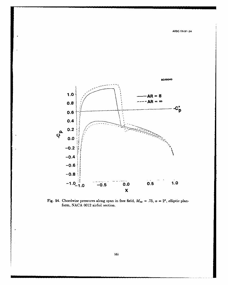
AEDC-TR-9 1-24
SC49040
1.0-AR = 00.8
I Ip0.6
0.47
0. 21.0 -k
-0.2N-0.4-
-0.61
-0.8
-1.0,1.0 -0.5 0.0 0.5 1.0
xFig. 94. Chordwise pressures along span in free field, M, .75, a =2*, elliptic plan-
form, NACA 0012 airfoil section.
161

AEDC-TR-91 -24
SCA9039
1.2--
I---------------------- C
0.
-0.2"/~
-0.4'AR 8.FREE FIELD
AR 8,FREE JET
-0.8!;
-101.0 -0.5 0.0 0.510
x
Fig. 95. Mean chordwise pressures in free jet, M~=.75, a = 20, elliptic planform,NACA 0012 airfoil section.
162

AEDC-TR-91 -24
-1.2 AR- SC-13W6T
- ,0.2 C) I
C 0. I - 04o z.
0.88
1.0.-1.0z -0. 0. 0.51.
0.63

AEDC-TR-91-24
W262 7 '/3 (3-93)
where W0o at x = -oo is assumed to vanish. If lateral symmetry W(x*,O) = W(x*, -8)is assumed, where 0 is measured from the intersection of the vertical plane of symmetryand the interface, W can be represented as the Fourier series (3 - 48b) where the W. aregiven after Eq. (3 - 49). On the basis of the analysis given in Section 3.1.2 the additionaldownwash W on the loaded line due to the interaction of the trailing vortex system with thewalls or interface can be represented by a superposition of two effects. If wo correspondsto the downwash increment a,,sociated with a free jet and w, is an increment associatedwith a pressure specification, then
w = w0 --w, = W(0, 0, z*) , -B < z* < B. (3- 94)
In terms of notation used in the code modules related to PHIl, w 4 tint. Based on theanalysis described in Section 3.1.2
1 00 J00-E_ n(-l)n J,(jz*) e- n" '
*1 IWn(x*)dx*, (3- 95)
W1n=1,3,5,...= J.(ins) 00
where K is the transonic similarity parameter, and j,,, are the zeros of the Bessel functionsJn.
In Section 3.1.2, approximations for the inner integral have been used that suggestthat the downstream features of the interface pressure do not contribute strongly to wl.Because of the substantial exponential factor in the integrand, (3-95) can be approximatedby including only the first term in the inner sum to give
w - 00 n l(Jlz*) eini2-'Wn(x*)dx*. (3-96)1=,3,5,-.. J'(i1) fc0
Equation (3 - 96) has been used to evaluate a special interface pressure distribution whichhas some features of those discussed in summaries of Calspan AEDC WIAC related effortcontained in Refs. 46 and 47. The model interface pressure distribution used with thegeneralized HIAR code is
cP, = C2e-gn(x*) {1 + el cos9}, -oo <x " < o (3 - 97)
where el1 and E2 are constants, and sgn(x) = 1 for x > 0, -1 for x < 0. Equation (3 - 97)implies that
W(X) = 2 (1 + e1 cos8)e - I ', (3 - 98)-232/3(3
W (*) = V2 - 1* (3 - 99a)262/3
164
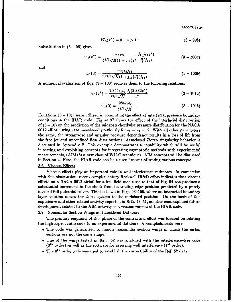
AEDC-TR-91-24
W.(x*)=0, n > 1. (3-99b)
Substitution in (3 - 96) gives
J-E2 i(jiiz*) (3 - lOOa))= 2/3vrK(1 +jlz* J (j1 1)
and(0-Cl2ll (3 - 100b)
wi(0) = 262/3V7?( ] +jii)J(jii)
A numerical evaluation of Eqs. (3 - 100) redaces them to the following relations:
1.855e1 62 J(3.832z*) (3 - 101a)wil(z*) -="( 0a62/31k Z
wi(O) / 984ce2 (3 - 101b)
b2/3VXK-
Equations (3 - 101) were utilized in computing the effect of interfacial pressure boundaryconditions ir= the HIAR code. Figure 97 shows the effect of the interfacial disfributionof (3 - 10) on the prediction of the midspan chordwise pressure distribution for the NACA0012 elliptic wing case mentioned previously for e1 = C2 = .2. With all other parametersthe same, the streamwise and angular pressure dependence results in a loss of lift fromthe free jet and unconfined flow distributions. Associated Zierep singularity behavior isdiscussed in Appendix B. This example demonstrates a capability which will be usefulin testing and exploiting concepts for integrating asymptotic methods with experimentalmeasurements, (AIM) is a new class of WIAC techniques. AIM concepts will be discussedin Section 4. Here, the HIAR code can be a usem! means of testing various concepts.3.6 Viscous Effects
Viscous effects play an important role in wall interference estimates. In connectionwith this observation, recent complementary Rockwell IR&D effort indicates that viscouseffects on a NACA 0012 airfoil for a free field case close to that of Fig. 94 can produce asubstantial movement in the shock from its trailing edge position predicted by a purelyinviscid full potential solver. This is shown in Figs. 98-100, where an interacted boundarylayer solution moves the shock system to the midchord position. On the basis of thisexperience and other related activity reported in Refs. 48-51, another contemplated futuredevelopment related to the AIM activity is a viscous version of the HIAR code.
3.7 Nonsimilar Section Wings and Lockheed DatabaseThe primary emphasis of this phase of the contractual effort was focused on relating
the high aspect ratio code to an experimental database. Accomplishments were:
e The code was generalized to handle nonsimilar section wings in which the airfoilsections are not the same shape.
* One of the wings tested in Ref. 52 was analyzed with the interference-free code(Oth order) as well as the software for assessing wall interference (1it order).
* The 0 th order code was used to establish the correctibility of the Ref. 52 data.
165

AEDC-TR-91 -24
SC-.2-6T-1.2
-1.0 ........
.0.4 .... . ....
-0.4
.... AR = 8FREE FIELD0.6 --- AR =8FREE JET
0.8 P RESSURE B.C.*,-'
1.0-1.0 -0.5 0 0.5 1.0
x
Fig. 97. Chordwise pressures at midspan with pressure boundary condition, ellipticplanform wing NACA 0012 airfoil, M,, = 0.75, a = 2*, p = 1.05,AR = 8, c, = 2 =.2.
166

AEDC-TR-9 1-24
NACA 0012 AIRFOIL Moo=0.799, SC29
a=2.26*, 1650 ITERATIONS
-- ----------------------
0
C0 0 ~ c 0
- 1 0 EXPERIMENT
-20 0.25 0.50 0.75 1.00
x/L
Fig. 98. Comparison of predictions from viscous interacted full potential equation solverand experiment.
167

AEDC-TR-91 -24
83423882.00-
1.20-
0.40-
y
- 0.40-
-1.20-
-2.00-1.92 -1.14 -0.365 0.415 1.20 1.98
x
Fig. 99. Densty level lines for inviscid flow - shock at trailing edge, NACA 0012 airfoil,M,., = 0.799, a = 2.260, 1650 iterations.
168
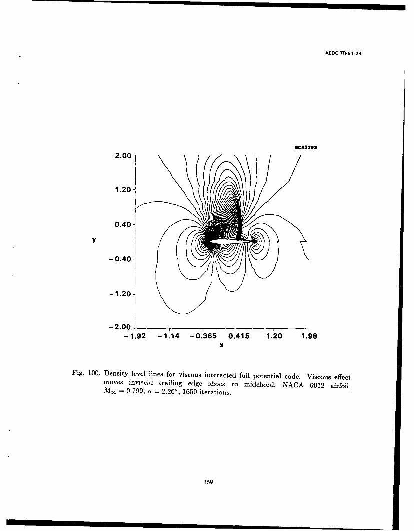
AEDC-TR-91-24
80423832.00
1.20-
0.40-
-1.20
- 2.00, ...
-1.92 -1.14 -0.365 0.415 1.20 1.98K
Fig. 100. Density level lines for viscous interacted full potential code. Viscous effectmoves inviscid trailing edge shock to midchord, NACA 0012 airfoil,M, = 0.799, a = 2.260, 1650 iterations.
169
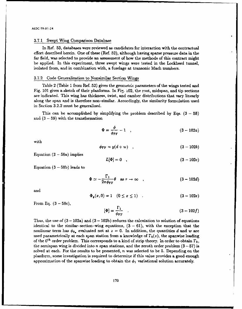
AEDC-TR-91-24
3.7.1 Swept Wing Comparison Database
In Ref. 53, databases were reviewed as candidates for interaction with the contractualeffort described herein. One of these (Ref. 52), although having sparse pressure data in thefar field, was selected to provide an assessment of how the methods of this contract mightbe applied. In this experiment, three swept wings were tested in the Lockheed tunnel,isolated from, and in combination with, a fuselage at transonic Mach numbers.
3.7.2 Code Generalization to Nonsimilar Section Wings
Table 2 (Table 1 from Ref. 52) gives the geometric parameters of the wings tested andFig. 101 gives a sketch of their planforms. In Fig. 402, the root, midspan, and tip sectionsare indicated. This wing has thickness, twist, and camber distributions that vary linearlyalong the span and is therefore non-similar. Accordingly, the similarity formulation usedin Section 3.2.2 must be generalized.
This can be accomplished by simplifying the problem described by Eqs. (3 - 58)and (3 - 59) with the transformation
p = L 1FF , (3 - 102a)
withOFF =y(d+w) (3 - 102b)
Equation (3 - 58a) impliesL[t= 0 , (3 - 102c)
Equation (3 - 58b) leads to
17 21F F asr--oo , (3 - 102d)
andtV(X,0)=l (0<5X<l) (3 -102e)
From Eq. (3 - 58c),
[§] = r, (3- 102f)
Thus, the use of (3 - 102a) and (3 - 102b) reduces the calculation to solution of equationsidentical to the similar-section-wing equations, (3 - 61), with the exception that thenonlinear term has Oo. evaluated not at z = 0. In addition, the quantities d and w areused parametrically at each span station from a knowledge of ro(z), the spanwise loadingof the 0 th order problem. This corresponds to a kind of strip theory. In order to obtain r0 ,the semispan wing is divided into n span stations, and the zeroth order problem (3 - 57) issolved at each. For the results to be presented, n was selected to be 5. Depending on theplanform, some investigation is required to determine if this value provides a good enoughapproximation of the spanwise loading to obtain the 01 variational solution accurately.
170

AEDC-TR-91-24
Table 2. Wing Model Geometry (from Ref. 52)
WING
A B C
AR 8.0 3.8 2.6
x 0.4 0.4 0.3
Ac/4, deg. 25.0 30.0 38.4
er, deg. 2.76 2.50 2.38
at , deg. -2.04 -4.00 -5.79
(tic)r, % 12.0 6.0 7.0
(t/c) t, % 12.0 6.o 11.0
S/2, cr2 (in2) 528.0 (81.8) 530.0 (82.1) 523.0 (81.0)
b/2, cm (in.) 45.7 (18.0) 31.8 (12.5) 26.1 (I0.26)
Cr, cm (in.) 16.351 (6.50) 23.88 (9.40) 30.83 (12.14)
cn (in.) 6.60 (2.60) 9.55 (3.76) 9.25 (3.6L)
MAC, cm (in.) 12.26 (4.825) 17.71 (6.97 ) 21.95 (8.642)
YMAC, cm (in.) 19.59 (7.714) 13.60 (5.355) 10.68 (4.:CE-;
171

AEDC-TR-91 -24
SC50720
21" 0.3i5"if 101
Figure 101. Planforms of tested wings (from Ref. 52).
172

AEDC-TR-91-24
SC50716
=0. 0
_____- WING REFERENE PLANE
1. 0
Figure 102. Wing A airfoil sections (from Ref. '2).
173

AEDC-TR-91-24
3.7.3 Results
Chordwise pressure distributions on the swept wing (Wing A) configuration of Ref. 52were computed at various angles of attack a, and Mach number M. To achieve rapid con-vergence, the streamwise grid was clustered near the blunt leading edge. To demonstratea typical calculation, Figs. 103 and 104 show the effect of wall interference and finite spancorrections on the chordwise pressures of Wing A at nearly midspan, and at two angles ofattack. The largest corrections appear to he near the shock at a = 00. By contrast, themore supercritical case corresponding to a = 10 shows a greater extent of the corrections.For both incidences, they are most pronounced on the upper wing surface.
In Ref. 30, modifications to the boundary value problem (3 - 57) are discussed for ayawed wing. The analysis shows that these changes occur in the far field for the three-dimensional 1 t order perturbation flow and in both the far field and equations of motionfor the 2nd order flow.
The HIAR code is based on a theory not designed for swept wings. This is becausethe dominant approximation of the inner flow assumes that all spanwise stations are ap-proximately two dimensional. If a discontinuity occurs in the slope of the leading edge, alocal three-dimensional flow occurs, nullifying this assumption. Such discontinuities occurat the root apex and tips of swept and other kinds of planforms. More general cases arecranked shapes. Asymptotic procedures are under consideration to treat these corner flowsand involve "canonical" numerical problems for the nonlinear flow near the corner. Thesecanonical problems remain the same for planform changes away from the corner.
In spite of this limitation, it was of interest to assess the correctability of the Wing Aresults using the 0 th order code. Figures 105 and 106 indicate chordwise pressure compar-isons of our 0 th order code with data from Ref. 52. In both figures, the effective tunnelMach number and angle of attack were modified to match the data. The similarity of thepressure distributions suggests the correctability of the test data. In Fig. 105, the influenceof shock-boundary layer interaction is not as great as in Fig. 106. For treating viscouseffects more effectively, under complementary IR&D funding, the contractor has developedan interactive boundary layer code based on Green's Lag Entrainment model that wouldpresumably reduce the effective increment in K associated with the combined Mach, angleof attack corrections used in Figs. 105 and 106. This was used to obtain the previouslydiscussed results indicated in Figs. 98-100.
3.7.4 Discussion
In comparisons such as Figs. 105 and 106, what needs to be analyzed are the combinedeffects of sweepback and viscous interactions on the interference. In Ref. 29, the similarityparameter K was allowed to vary from the 0 th order flow to the 1 t order wall interferenceflow. This flexibility should be investigated with the aim of systemizing the correctionsthat can be obtained through studies of the type associated with Figs. 105 and 106. Thevariation of K is expressed in a perturbation form related to the asymptotic expansion ofthe perturbation potential 0. This perturbation gives the flexibility of varying the tunnelMach number and geometric angle of attack to correct or simulate free field conditions.
174
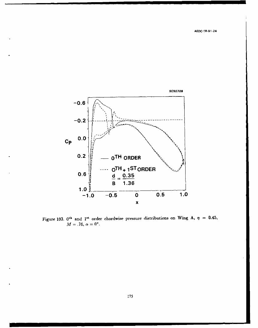
AEDC-TR-9 1-24
SC50708
-0.6
- 0 2 ---------- -----.
0,0 SCp 0.0 "
0.2 TH ORDER
0.6 --- OTH + 1ST ORDER0.6d 0.35
B 1.36
-1.0 -0.5 0 0.5 1.0x
Figure 103. 0 th and 1"t order chordwise pressure distributions on Wing A, Y7 = 0.45,
M = .76, a = 00.
175

AEDC-TR-91 -24
SC50709
-0.6- 0TH ORDER
-0. - ---------------------- ------------------ OWTH1TRE
__ d _0.35
Cp ~ B 1.36
-1.0 -0.5 0.0 0.5 1.0x
Figure 104. 0 th and I" order pressure distributions on Wing A, Y = 0.5, M =.76, a~ 10.
176

AEDC-TR-91-24
SCS0711
A A 0 TH ORDER CODEA1
M = 0.72, a V
-1.0 A UPPER SURFACE EXPERIMENTLOWER SURFACE M =0.76, a = 2.95'
-0.6
Cp -0.2
0.2
0.6
1.0!-1.0 -0.5 0.0 0.5 1.0
X
Figure 105. Comparison of theoretical and experimental chordwise pressures for Wing A,Y7= 0.5, tested at M = 0.76, a = 2.95.
177
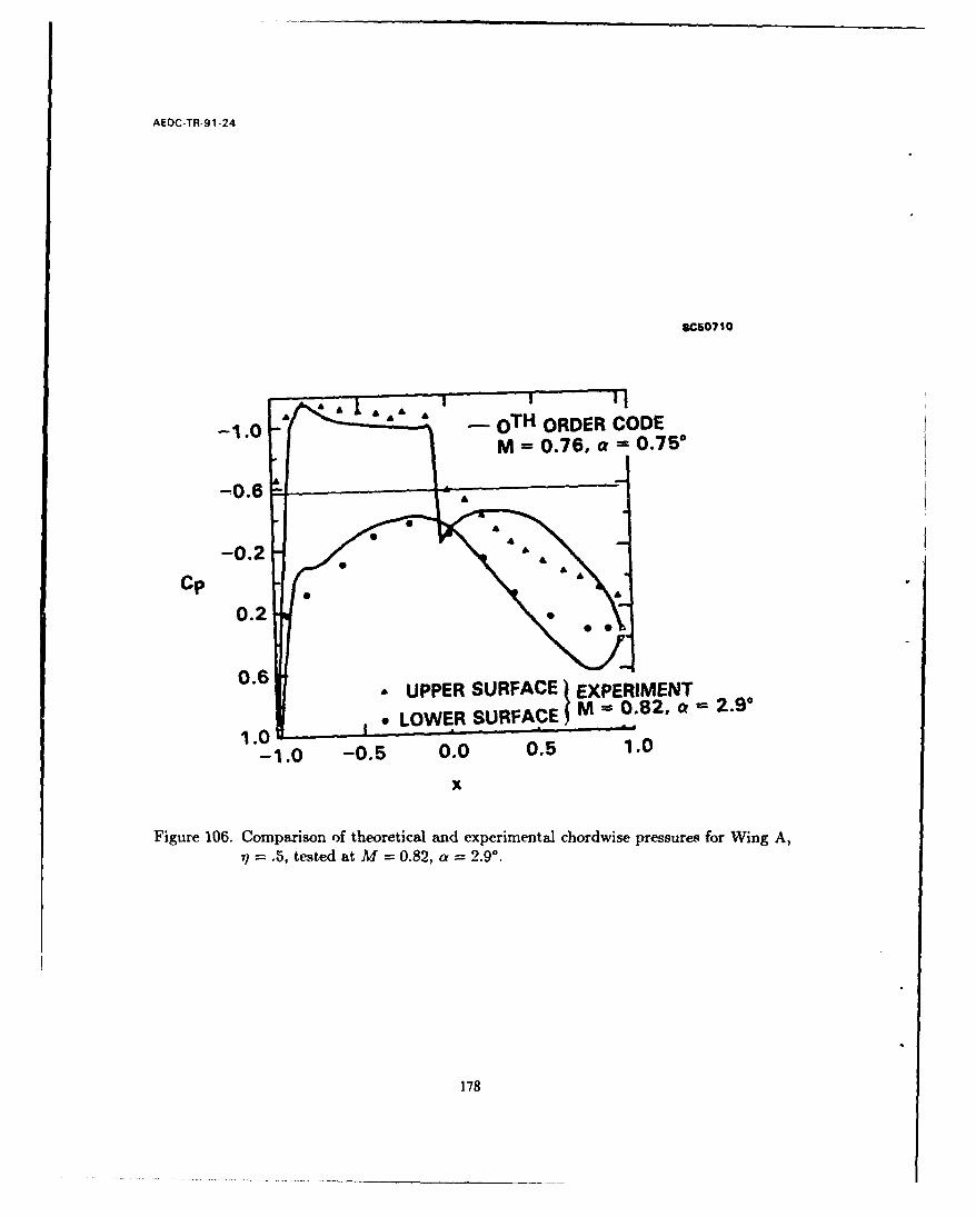
AEOC-TR-91 -24
3050710
-1.0 - TH ORDER CODEM =0.76, 0.75*
-0.6
-0.2Cp
0.2
0.6& UPPER SURFACE~ EXPERIMENT
* LOWER SURFACE M = 0.82, a2.901.0 -&
-1.0 -0.5 0.0 0.5 1.0
x
Figure 106. Comparison of theoretical and experimental chordwise pressures for Wing A,
'?= .5, tested at M =0.82, a = 2.90.
178
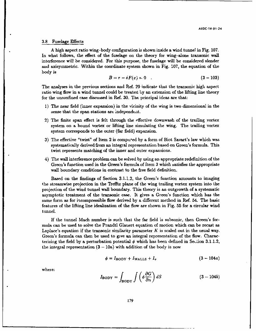
AEOC-TR-91-24
3.8 Fuselage Effects
A high aspect ratio wing-body configuration is shown inside a wind tunnel in Fig. 107.In what follows, the effect of the fuselage on the theory for wing-alone transonic wallinterference will be considered. For this purpose, the fuselage will be considered slenderand axisymmetric. Within the coordinate system shown in Fig. 107, the equation of thebody is
B=r- F(x)= 0 (3-103)
The analyses in the previous sections and Ref. 29 indicate that the transonic high aspectratio wing flow in a wind tunnel could be treated by an extension of the lifting line theoryfor the unconfined case discussed in Ref. 30. The principal ideas are that:
1) The near field (inner expansion) in the vicinity of the wing is two dimensional in thesense that the span stations art independeat.
2) The finite span effect is felt through the effective downwash of the trailing vortexsystem on a bound vortex or lifting line simulating the wing. The trailing vortexsystem corresponds to the outer (far field) expansion.
3) The effective "twist" of Item 2 is compu'ed by a form of Biot Savart's law which wassystematically derived from an integral representation based on Green's formula. Thistwist represents matching of the inner and outer expansions.
4) The wall interference problem can be solved by using an appropriate redefinition of theGreen's function used in the Green's formula of Item 3 which satisfies the appropriatewall boundary conditions in contrast to the free field definition.
Based on the findings of Section 3.1.1.2, the Green's function amounts to imagingthe streamwise projection in the Trefftz plane of the wing trailing vortex system into theprojection of the wind tunnel wall boundary. This theory is an outgrowth of a systematicasymptotic treatment of the transonic case. It gives a Green's function which has thesame form as for incompressible flow derived by a different method in Ref. 54. The basicfeatures of the lifting line idealization of the flow are shown in Fig. 55 for a circular windtunnel.
If the tunnel Mach number is such that the far field is subsonic, then Green's for-mula can be used to solve the Prandtl Glauert equation of motion which can be recast asLaplace's equation if the transonic similarity parameter K is scaled out in the usual way.Green's formula can then be used to give an integral representation of the flow. Charac-terizing the field by a perturbation potential 0 which has been defined in Se.Lion 3.1.1.2,the integral representation (3 - 10a) with addition of the body is now
I -BODY + 'WALLS + Iv (3 - 104a)
where:
BODY -dS (3- 104b)JBODY I 5n]
179

AEDC-TR-91-24
SC45484A-MODEL
14 y INNER LIMIT
REGION OF OUTER
,,._.." //WAKE
TUNNEL BOUNDARY
Fig. 107. Confined high aspect ratio wing-body model.
180

AEDC-TR-91-24
and 'WALLS and I,, are defined in (3 - 10b) and (3 - 10c) and G = 0 on the walls asin Section 3.1.1.2. Therefore, if a free jet wall boundary condition 4 = 0 is considered,'WALLS == 0. For convenience, the thickness effect of the wing will be neglected in whatfollows. The analysis can be easily extended to include it.
it will be seen that the principal effect of the body is to modify the integral I. in(3 - 11a). rhis causes a change in the finite-aspect-ratio downwash all along che loadedline. A m3rc local effect occurs in the near field at the wing-body junction in the case of theflow near the tips or a kink at the center of a planform. In these regions, the assumption efindependence of spanwise sections is invalid. The resulting fully three-dimensioal flowsare assumed to lead to only a secondary influence on wall interference and wi. thereforenot be considered in what follows. The main focus will be the calculation of 1. Prior toits calculation, we note that 'BODY is given by
'BODY = linj - . 27rpGBODYd4 (3- 105)
By linearity of the outer flow field, the body is assumed to be characterized by a line sourcewhich is siuperir- posed on the trailing vortex sheet flow shown in Fig. 55. Hcre,
lim p -- A=( ) (3-106)P-0O Op 2wr
whe.e A is the local cross sectional area. Because of the superposition property, a moregeneral fuselage shape can be considered. For such a configuration, (3 - 105) and (3 - 106)would still be valid.
In a free field,1 1
G -(3-107)47r X - V ) + ( - 01+ (Z -C
where for y, 77, z, C will hereinafter signify scaled coordinates.
For free jet boundary conditions on a circular wall, it was shown in Section 3.1.1.2Lhat
G- 2/ 2 cosn6-' e-Anhk-IJn(Ankr)Jn(AnakP) (-1
k =~ [1(~kA] e (3 - 13')
where the Jn are Bessel functions and Ank their zeros in accord with definitions givenearlier, and by symmetry the 0' argument given in (3 - 13) is omitted. Because of axialsymmetry, the effect of /BODY on the finite aspect ratio downwash effect will be zero.
To treat I, the result obtained from a systematic approximation procedure for thewing-alone case will be generalized. The generalization will be obtained by modifying theimaging solely in the Trefftz plane. Accordingly, the doublet sheet interaction with the freejet tunnel boundaries will be considered as depicted in Fig. 108. As in Section 3.1.1.2, theeffect of the line doublet is obtained by superposition of individual elements. A circular
181

AEDC-TR-91-24
cross section body is analyzed herein. More general cross sections can be handled by thetechniques described in Refs. 49 and 51.
To expedite the solution, only slender bodies in the sense that the maximum bodydiameter is small compared to the wing span will be treated. In fact, in the outer limitcertain stretched coordinates were introduced in Ref. 29. Denoting the span in units ofthe chord as b, these are
* = *= * B-6 1 1 3 b fixed as6 -0 (3-108)B ' B' b
Accordingly, E =.-"-- Obviously, other choices are possible besides using 6 as the bodymaximum thickness in (3 - 1). This option gives a region of transonic flow around thebody Lhat has lateral dimensions of 0(b-1).
To obtain the image of a doublet in the annular region e < r* < p shown in Fig. 108,perturbation methods are used. Here, r* = y' + z*2 . Two cases can be identified:
(i) =o(1)(ii) 0 = (E)
Case (i)
Denoting the complex potential as F(Z) = (z, y) + io(z, y) with Z = z + iy, wherethe stars on y and z will be dropped, the appropriate expression for F is
2s'riF = z;2+ (Z -e- -( A )Z-(3-109)
1
In (3 - 109), (Drepresents the doublet, ®its "reflection" in the tunnel boundary r = p,() is a compensation term to make the body a stream surface, and @is a constant added tomatch the Case (ii) expression for ( in an overlap domain of mutual validity. This featurewill be used to obtain a uniformly valid representation in C. Term (is associated with thebehavior
(!)+®=" z as z,
and the circle theorem for homogeneous Dirichlet conditions. Thus if A = + *
2=A(Z-)
182

AEDC-TR-9 1-24
SC48993
Fig. 108. Projection of doublet sheet in Trefftz plane.
183

AEDC-TR-91-24
- 2
and since Z 1 on r = e, then
®+ ®+ Q = A(Z --Z)so that
Re(O+ Q+ Q) = 0
which is the desired property.
It is important to note that the reflection term Q does not spoil the boundary con-dition on the tunnel boundary IZI =p.
Case (ii)
For this case,
2rF 1 ____Z - 2 Z L -2 ( 2- (3-110)
In (3 - 110), Term 3)' plays the same role at IZI = p that Qdid in (3 - 109) at IZI = E.
Equations (3 - 109) and (3 - 110) can be used for separate ranges of a convolutionintegral representing the perturbation potential of the doublet sheet in the Trefftz plane. Toremove arbitrariness associated with the cutoff between Case (i) and Case (ii), a combineduniformly valid expression in C is preferred. This is obtained for the function
1U(Z;c) =21riF - (3-111)
An intermediate limit is considered in which
(=_ fixedas e-*017
where e << 77(c) << 1.
Thus, for both Case (i) and Case (ii),
U=_-z (3-112)
The uniformly valid representation is therefore the sum of the representations for Case (i)and Case (ii) minus the common part given by (3 - 112). The resulting expression is
2-riF Z- _ +L2{z - +--- (3-113)
184

AEDC-TR-91-24
Taking the real part in (3 - 113), the resulting expression for I, is:
I= - f -(C) 1 1 + __4v (Z - ()2 + y2 ( 2+ y 2 + (Z 2 )I(C{(z 2 + 12 ~ 2
+ ____ Z2 2(Z 2)2+ ] (3 -114)
C2 2
3.8.1 Discussion
Equation (3 - 114) represents the downwash expression associated with finite spanfor a high aspect ratio wing-body combination in which the body maximum thickness isa small fraction of the span. This expression is the generalization of that being used forthe inner solution far field for the wing-alone code. It contains interactions between thetunnel boundaries and the body. It is clear that the most important contribution is when
o(8).
185
AEDC-TR-91-24
4. ASYMPTOTICS INTEGRATED WITH MEASUREMENT (AIM)INTERFERENCE ESTIMATION METHODS
Analytical and computational techniques were described in the previous sections topredict transonic wind tunnel interference over slender and high aspect ratio models. Thesemethods are oriented to interference prediction stric '7 from a knowledge of the tunnel andmodel geometry as well as the flow parameters such as test section Mach number. Theyare based on an inviscid approximation of the flow. However, by allowing the boundaryconditions on an outer wall or cylindrical interface to correspond to the specification ofpressure, viscous ,.nd other phenomena may be indirectly incorporated into the anal,-sisin accord with methodology developed by workers at AEDC, NAE Ottawa, NASA, andelsewhere. For purposes of the following discussion, such techniques will be grouped underthe category of Wind Tunnel Interference Assessment/Correction (WIAC) methods. Bycontrast to the methodology in Sections 2 and 3, these approaches combine the analysis andcomputation with experimental methods to determine the magnitude of the interferen'e aswell as the feasibility of accounting for the interference either by simulating an interference-free condition corresponding to the test environment or providing some sort of post-testcorrection to the data.
In what follows, procedures are described that can augment the effectiveness of WIACconcepts. They exploit the theoretical knowledge developed under this contract describedearlier in this report as well as experimental measurements in the determination of wallinterference. The scope of the discussion is to outline the basic concepts. A more detailedfeasibility study as well as proof of concept is intended as future effort.
4.1 Interference on Moderate and Low Aspect Ratio Configurations
As described in Ref. 29 and elsewhere, the two variable method (TVM) provides abasis for simulating the effective body shapes in the tunnel which may differ from the"hard" physical geometry of the model due to viscous interactions and other effects. Ifthis representation is assumed to be the same in the free field, then its knowledge frommeasurement and computation can be utilized with further computation to obtain the freefield aerodynamics or the interference. Existing transonic TVM's such as those describedin Ref. 13 typically employ a second measurement on the interface to establish the effectivebody shape with an iterative computational inverse procedure. In the inverse method, afirst guess is successively refined in a feedback loop to satisfy the second interface condi-tion. A concept has been developed in the contract to avoid this loop or accelerate itsconvergence. Application to nonaxisymmetric compact configurations that satisfy a classof requirements which may be of considerable practical WIAC utility has been investigated.
The method is motivated by slender body theory. Using previous notation in whichak = angle of attack, 6 = maximum thickness ratio, b = semispan, h = characteristic walllateral dimension, the flow over a test article shown in Figs. 109 and 110, and given by
r = 6F(z,6) (4-1)
186

AEDC-TR-91-24
is considered, where the normalized cylindrical coordinates
X z - r (4-2)C C C C
are employed and c is a characteristic body length. In the inner near field, close to themodel as described in Refs. 29 and 30, the following asymptotic expansion is assumed tobe valid for H = h6 fixed*
x + 26 2 logbS,(X )+ 2 (X,*,z*;A) + 4 109421 (x, y*, z*; A) + 6 4 p 2(x, y*,z; A)U
(4-3)which is valid in the inner limit
Y1 _ M.2 axly* K= A= fixedas 6--*0 (4-4)
The "far field" of this inner expansion worked out in Ref. 30 is if r* = r/6 -400
W, = S, (x) logr* + g(x) + Dl(z)cos8 + E 1 (x)cos 20r* + r*2 +(4 -5a)r* r*
WP21 = 2SS'logr* + 921(X) + 2S2(x) +.." (4 - 5b)
VP2 = SSI log2 r* + 82(x) log r* + g 2(x) +'" (4 - 5c)
where if A*(x) = normalized cross sectional area, S1 = 2 and S2 can be found fromintegral theorems based on the inner bomdary value problems but will not be consideredfurther here. This approximation is nonuniform with respect to r*. Two other approxi-mate representations are required to overcome this nonuniformity. For H = fixed, and acylindrical wall, there is an outer region in which the asymmetries relax to nonlinear axialsymmetry in a manner that has been discussed in Refs. 29, 30 and elsewhere**. Prelimi-nary studies based on integral equation asymptotics and particular solutions indicate thatthe wall reflections are regular functions of r* which do not perturb the singular behaviorthat controls matching with another representation needed in an intermediate domain toobtain consistent approximations in the higher orders. This fact has implications on themagnitude of the lift interference.
From Ref. 30, the outer expansion of 41 is:
4t = x+ 2g(x,6, ;K,A,H)+b4109602 1 +640 2 +... (4- 6a)
* The H --, oc approximation made in Ref. 29 will be suppressed.
•* This property can be extended to mildly noncircular test sections such as octagonalshapes or measurement interfaces that are sufficiently distant so that the angular pertur-bations are weak. This can be formalized asymptotically.
187

AEDC-TR-91-24
SC83-22869
, /,
Fig. 109. Slender vehicle confined inside cylindrical wind tunnel walls.
188

AEDC-TR-91-24
r=0(6-SC45485MODEL.
INNERREGION
Xh
iiiREGION r-=OI
OUT ER RE GION
INTERFACE
Fig. 110. Front view of wind tunnel model confined by cylindrical walls, showing importantregions.
189
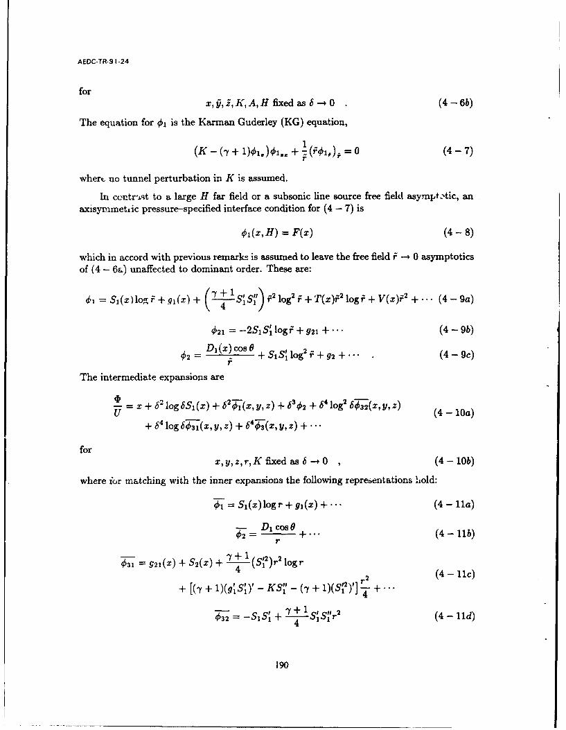
AEDC-TR-91-24
forx, P, i, K, A, H fixed as b --+ 0 (4 - 6b)
The equation for 01 is the Karman Guderley (KG) equation,1
(K-(- + 1 ) + , =0 (4-7)
whert no tunnel perturbation in K is assumed.
In cec'tr-.gt to a large H far field or a subsonic line source free field asympt.tic, anaxisy?-met-ic pressure-specified interface condition for (4 - 7) is
C1,(x, H) = F(x) (4-8)
which in accord with previous remarks is assumed to leave the free field F --+ 0 asymptoticsof (4 - 6a) unaffected to dominant order. These are:
951 = S (X) log +.gq (X) + + -- SS' si 21og2 f + T(X)f2 log f + V(X)F2 +' (4 -9a)
021 = -2SiS' log + g2 +" (4 - 9b)¢-Di(x) cos B
0 + SSlog2 f +g 2 +"" (4- 9c)
The intermediate expansions are
4- = x + b2 log bS1 (X) + b2T(x ' y' ) + A ¢ + 6' log2 6 - 2(x ' yz) (4- 10a)+ 6U log623xy,T) + 6Z(, (,4) +..
forx,y,z,r,K fixed as -0 , (4 - 10b)
where for matching with the inner expansions the following reprebentations hold:
;F= Sl(x) log r + gi(x) +. (4 - 11a)
DI cos 02 = DCos +" (4- llb)
r
3 9g21(x) + S2(X) + + 1(st2 )r 2 log r(4- 11c)
+ [(-f + 1)(g',S')' - KS"'-(-t + 1)(S'2)'] 4 +-'
--S1 + 1--S S'r 2 (4 - 11d)
190

AEDC-TR-91-24
E1 cos2 S
- r2 + SS log2 r+S 2(x)logr+g 2 (x) (4 - lie)
+ + S'Sr 2 log2 r + T(x)r2 log r + V(x)r 2 (4 - 1f)
For purposes of assessing drag interference, the key idea in one possible AIM TVM conceptbeing evaluated is that Eqs. (4 - 11) can be used to determine the "effective body" inter-action with nonlinear outer flow field. For example, it is envisioned that (4 - 11a) canbe used to determine the effective source strength Si(x) by a simple radial differentiation,i e.,
T = b + O(b3) r S(x) (4-12)U r
and a measurement of the radial velocity 4,r on an interface surface r = 0(1) at each xstation. The function Si(x) can be used with the boundary condition associated with thedominant term of (4 - 9a) to obtain the solution of (4 - 7) subject to (4 - 8), where F canbe obtained from pressure measurements as
F 2 C,(x, H)dx (4- 131b2
The solution of the outer KG problem will give the free field drag and the interference.For example, under mild restrictions on the equivalent body of revolution source strengthdistribution Sl (x), the free field wave drag D is
pDU2 = 2rb4 S(x)g(x;K)dx (4-14)
based on a momentum theorem given in Ref. 30. In (4 - 14), the function gi is computedfrom the numerical solution of the free field KG problem.
In accord with previous remarks, it is envisioned that this approach may be generalizedto weak deviations about axial symmetry on a measurement interface in the outer regionf = 0(1).
Analyses of the free field structure for the highly and intermediately loaded caseshave been given in Refs. 18 and 55, respectively. Reference 48 describes the case where
K - 1-M2 , with el 1 a2 In 1 , and Ref. 21 considers the thickness 6 = O(ei). For
Ref. 48, in contrast to the case described in detail above, the first order term in the nearfield is approximately a dipole. No intermediate expansion is needed to match with theouter representation which still relaxes to KG axial symmetry to dominant order. However,the effective source strength Si, rather than being controlled by the rate of change of cross-sectional area A*(x) as in the weakly loaded case, is given by:
S= -= +1 (xy'(x) (4-15)2 (21r) 2
191

AEDC-TR-91-24
where 41(x) is the cumulative free field lift up to a station x, which can be computed byJones' theory. For a cambered, zero-thickness wing on (0 < x < 1, -ZLE !_ z < ZLE),
for which y = af(x), fi(x) = -7rf'(x)zLE(X). Studies are in progress of the matching toassess what is the role of the wall reflections on the inner flow field structure and theirimportance relative to the interference lift. For drag of a zero thickness configuration, theeffective source strength distribution may be inferred from the measurement procedurepreviously described, since the outer zolution has the same dominant behavior giver by(4 - 11a), in spite of the different interpretation in (4 - 15).
The relaxation to the structure given by (4 - 9a) in about the r = O scale of thelift dominated theory has been corroborated with zonal gridding procedures and free fieldEuler calculations of K. Szema which were funded under another program using codes andalgorithms developed by S. Chakravarthy. The F-14 configuration shown in Fig. 111 wasanalyzed with simulated flow-through inlets at Mo, = .8, and a = 13.50. The isobars areshown in Fig. 112. There is also a suggestion of near field __ behavior in the contourswhich are however skewed by strong tip vortices.
The relaxation shown in Fig. 112 is a suggestion of the feasibility of the radial velocityunfolding concept previously indicated to obtain the effective source strength SI. Onepossible application of the method could be the cruise missile configuration discussed inRef. 47.
4.2 High Aspect Ratio Configuration WIAC Method
Considering the high aspect ratio arrangement shown schematically in Fig. 113, at awake station PQ associated with a near field limit of the outer solution, downwash due tothe vortex sheet reflected in the tunnel walls has been derived and discussed in connectionwith the lifting line theory of transonic wall interference in Section 3.1.1.2. Suppressing theadditional fuselage upwash effect and its interaction with the walls, which can be handledby conformal mapping procedures, the net downwash in a y = 0 downstream plane of thewing alone is
w 4j - -z(z I d(-+ w(z) (4-16)
where using previously defined notation /ps H/B = L, H = 6b1 /3h, B = ON/3 b, 'Y isproportional to the free field infinite aspect ratio sectional lift coefficient and w, is thedownwash effect associated with deviation of the pressure field on the interface from zeroperturbation pressure, where from Section 3.1.2, if the interface pressure is Cp,
W(x',O) =fCP(;,,GdW(X* 0) = Cp, (x*, H, 0) dx*
0 0-22/3
Wo( ) + EW.(x)cosnOn= 1
x=Hx* , 6" 3 y= Hy , i = b11 3 z Hz*
192

AEDC-TR-9 1-24
4
SC45487
Fig. 111. F- 14 configuration.
193
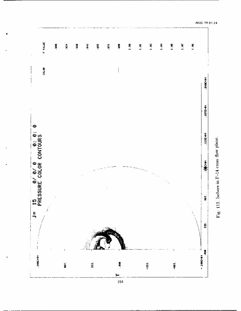
AEOC-TR-9 1-24
i 0! - W C! C! i. 0 * *
.
Ca
0
Li
CC
0
'GO
SI.
Clon
/ bb
I19

AEDC-TR-91 24
MODELy INNE R LIM IT
REGION OF OUTER
tQ
"Vo WAKE
-INTERFACE
Fig. 113. High aspect ratio wing model.
195

AEDC-TR-91-24
withWo= jW(x-,)d
W. =2 W(x:*,9)cos nOdOlr
and 1 Ji Uoz* 00w] , / z- E n(-l) en=13,5- - S J. l) foo
where K is the transonic similarity parameter and the j, 1 are the zeros of the Besselfunctions Jn(z*).
Equation (4 - 16) can be used to determine the free field lift and span loading as follows:
1. Measure the left hand side w at PQ. A generalized form of (4 - 16) applies at y : 0and the measurement could be made above or below y = 0, if this is more practical.
2. Equation (4 - 16) can be inverted once and for all numerically and presumably alsoanalytically with a Green's function based on conformal mapping.
3. An analytic inversion of (4 - 16) can be used to compute 7'(() by a quadrature. Thiscould be interpreted as the "effective" span loading associated with viscous effects.
4. The function -y'(() in Item 3 can be used to compute the free-field finite aspect ratiodownwash correction w0 , on the loaded line given by
1 B_ y(¢
woo = -- (4-17)
where the principal value of the integral is to be taken.
5. The HIAR code can be used with w.. to compute the free field span loading and lift.
4.2.1 Discussion
Steps 1-5 in the high aspect ratio AIM method sidestep the need for computationallyintensive three-dimensional simulations as well as time-consuming gridding preparation.It however requires a knowledge of the downwash field behind the model. This can bedone by a rake or other instrumentation. Once this is obtained, (4 - 16) can be invertedusing Fourier series or collocation methods. The approach indicated is by no means limitedto a downwash measurement. Other derivatives of the scheme can be conceived such asusing pressure measurements. Since the approach depends on the application of lifting linetheory, its elasticity with respect to moderate aspect ratio shapes needs to be assessed.This can be achieved by comparisons with three-dimensional numerical simulations andexperiment.
196

AEDC-TR-91-24
5. CONCLUSIONS, HIGHLIGHTS AND SUMMARY OF FINDINGS
Transonic wall interference asymptotic formulations developed under a previousAEDC contract, "Study of Asymptotic Theory of Transonic Wind Tunnel Wall Interfer-ence," (Coutract F40600-82-C-0005) have been computationally implemented. This ac-tivity motivated additional asymptotic studies and the development of AIM (AsymptoticsIntegrated with Measurement) techniques that are designed to extend the applicability ofthe computational and analytical methods.
Key findings and highlights of the effort are:
1. The "Area Rule" for transonic wall interference of slender airplane test articlesdiscovered in the previous contract, applies for pressure boundary conditions inthe large height limit, H --* o. Its validity tor pressure interface boundaryconditions needs to be assessed for H = O(1).*
2. The scalings associated with the gauge functions appearing in the formal asymp-totic expansions for the interference potential in the slender body limit agreeswith that deduced by Goethert in Ref. 56 using non-asymptotic methods andvalidated against experiment.
3. Pressure specified interface boundary conditions over confined, slightly subsonicslender bodies give an asymptotic triple deck structure resembling that arisingfrom free jet and and solid-wall, classical conditions, providing that the interfacecircumferential variations are mild. Such angular distributions are anticipated inthe sensible far field with circular or octagonal test sections, even for realistic,compact fighter configurations having appreciably asymmetric cross sections, butat moderate angles of attack. This occurs because of the strong three--dimensionalflow relief associated with this small average effective thickness ratio or charac-teristic flow deflection (6) regime and the associated rapid relaxation to axialsymmetry in the radial direction transverse to the freestream.
4. The inner deck has the usual Oswatitsch Equivalence Rule cross-flow harmonicstructure. For large height, the intermediate layer is a weak perturbation aboutfree field conditions, where the strength of the perturbation is o(H) asH --+ oo. In this region, matching with the outer deck shows that the effectof the pressure boundary conditions is felt in an average sense, i.e., only the firstfew harmonics of the circumferential variation are important. The outer or "wall"deck is an effective tube vortex reflection of the multipole representation of thetest article. Higher order approximations of the intermediate or central deck leadto -" terms in the equation of motion. However, the significant computational
082overhead of the resulting three dimensional formulation can be avoided since the0 variation is simple and can be factored out due to linearity. This leads to a
* The asymptotic treatment of these pressure conditions was undertaken over and above the
Work Statement of the current contract.
197

AEDC-TR-91-24
two dimensional (axisymmetric) formulation similar to that encountered in theFJSWCI (free-jet or solid wall cylindrical interface) problem, except with forcingterms (in the higher approximations). These can be readily treated with superpo-sition procedures that are allowable due to linearity of the variational interferenceequations.
5. With pressure interface boundary conditions, the H scaling of the similarity lawsfor ACp and ACD, respectively, the interference pressures and drag, are un-changed from the FJSWCI case. Again, in contrast to the H = 0(1) problem,but as in the FJSWCI case, the H scaling is known, eliminating the need to solvefoi new H's associated with different test facilities when all other paramieters areunchanged.
6. For solid walls, and for the H = 0(1) numerics, the structure of the upstreamand downstream far fields was determined. For a blunt or stinged base, a uniformsource flow at infinity results, in which 0 _ ±Cx as x -- ±00, where C -
body base area. For a closed body, 4 _ ±D as x --* ±00, where D=doubletstrength which consists of a linear part, proportional to the body volume, and anonlinear portion proportional to the average kinetic energy of the interferenceperturbation of the streamwise velocity component. It was expedient to avoidthis term in computational implementations for closed bodies. HomogeneousNeumann conditions were used at the inflow and outflow boundaries x = ±00rather than the doublet condition. This step was justified due to the exponentiallysmall higher order terms in the x --* ±00 far field expansion. This structure issimilar to two-dimensional flow solutions worked out in Ref. 57, in which the wallcondition "drives" a faster decay than the algebraic one associated with the freefield. The exponential rate of decay for the axisymmetric case of slender bodytheory differs from the two-dimensional airfoil case since these are eigenvaluesarising from the Sturm-Liouville problem for the Green's function and thesediffer in both situations.
7. Consistent with the contractual Statement of Work (SOW), Task 1.0, a codesolving only the FJSWCI case was developed. (Pressure boundary conditionshowever can be treated by the high aspect ratio code developed under Task 3.0.)Two solver modules (RELAX1 and RELAXV1) were developed to model the0th order free field basic flow and its 1st order wall interference perturbation,respectively. An excellent experimental validation of RELAX was achieved fora blunt nosed axisymmetric body tested by Couch et al. It is believed that anintrinsic element in obtaining this validation was the special procedure developedto discretize the boundary points near the logarithmically singular line f = 0 inthe inner Axis deck of the flow. In keeping with the thrust of the contractual effortthat combines the best features of asymptotics and numerics, these discretizationsused the inner expansion instead of a one term Taylor expansion with a remainderto characterize the nodes near f = 0.
8. Special techniques extending those originally developed by Small and Cole wereutilized to fit the shock in the numerical treatment of the interference perturba-
198
AEDC-TR-91-24
tion flow. Schemes were worked out to surround the shock by an "upright" notchhaving vertical and horizontal sides. This scheme which is easier to programand avoids subtle issues associated with an alternative method which actuallyfollows the shock curve with a "staggered notch" was computationally imple-mented. More effort is required to compare the effectiveness and accuracy ofboth approaches. An important issue is the accuracy of the discretizatiop of thevertical velocity component vi of the variational flow and the avoidance of un-necessary smearing out of the shock region beyond the normal Rankine-Hugoiliottransition zone if an upright notch is used. For slender bodies, this concern seemsto be relieved by the fact that the shocks are almost normal, since the freestreamMach number needs to be very close to unity to obtain a supersonic bubble ofany significant size. A study of the relative criticality of this issue for the highaspect ratio problem is also needed.
9. Other sensitivities of the numerical treatment of the interference field are theproper dimensions of the notch and the definition of the tip of the shock. Fcrthe two-dimensional airfoil case, Murman numerically investigated the formationof the shock as the envelope of the characteristics of the second family reflectingfrom the sonic line. Because of its steepness, this envelope is poorly defined. Thecalculations showed some sensitivity to this definition as well as the location ofthe position of the upstream and downstream vertical legs of the notch. Morework is needed to improve this part of the method. From experimentation and anexamination of the pressure profiles as well as the x discretizations, a four pointtransition seemed appropriate for the width of the notch for slightly subsonictunnel Mach numbers.
10. In a separately fundcd AFOSR effort, the structure of the triple point singularityat the foot of the shock was examined in connection with handling the pertur-bation Rankine-Hugoniot shock conditions at the notch, particularly at the foot.As a part of this, Cole and Malmuth in Ref. 38 analyzed a shock position invari-ance with Mach number discovered by the latter in calculations of the flow over aparabolic arc body. More work is needed to understand this phenomenon in freeand confined flows in connection with generalized Lavrentef-Bitsadze models.
11. Calculations for flow over a parabolic arc body at a freestream Mach number of.99 indicate that the wall perturbation flow has a very dominant spike localizedabout the shock region. The preshock influence is very weak compared to thepostshock influence. The shock spike phenomenon seems to control the entirestructure of the interference flow and there is rapid decay away from this region.
12. Allowing for a perturbation K1 in the similarity parameter K in the asymptoticexpansions for the perturbation potential provides flexibility in defining minimuminterference or interference-free conditions. A proof of concept has been obtainedin which interference-free conditions for the drag have been been defined for aparabolic arc body through alteration of the tunnel Mach number or its thicknessratio using methodology discussed in Section 2.18.
199
AEDC-TR-91-24
13. Lift interference is negligible compared to drag interference for the thickness dom-inant distinguished limit of the free field slender body basic flow.
14. Pressure specified boundary conditions include the same mechanism governingwall interference for high aspect wings as with free jet and solid wall boundaryconditions. Namely, the interaction is still primarily associated with the alterationof the downwash field on the loaded line (bound vortex) due to the interference ofthe walls or interface with the trailing vortex system. The effect of the variableinterface pressures can be handled by a superposition of a tube vortex and afree jet solution. The tube vortex corresponds to the interfacial pressure dataand is continuous across the wing wake. The sum of both solutions satisfies theboundary conditions of the complete problem. The tube vortex modifies thedownwash on the loaded line, i.e., the effective angle of attack along the span ofthe wing.
15. The interference downwash on the loaded line due to the imaging of the trailingvortex sheet into the walls or interface was analyzed to successfully accomplishTask 2.0 of the contractual effort. A Green's function method was developed toprovide an extremely powerful means of obtaining an asymptotically consistentapproximating sequence for the imaging. Properties of the Bessel functions ap-pearing in the integral or eigenfunction representation of this Green's functionindicate that even for the transonic case, the downwash field is essentially thesame as that for incompressible flow. In particular, it is the solution of a two-dimensional problem in the Trefftz plane infinitely far downstream. This problemreduces to the interaction of a two-dimensional vortex sheet distributed along theprojection of the wake in the Trefftz plane with the circular projection of thewalls or interface in this plane. Another Green's function which can be obtainedby the Melthod of Reflection involving inversion in a circle solves this problem.However, the expansions of the Bessel functions in the expression for the firstGreen's function give this interpretation directly. Corresponding information isneeded for choked and slightly supersonic tunnel flows.
16. Under Task 3.0, a code capable of handling high aspect ratio configurations wasdeveloped. As in the slender body code written under Task 1.0, an upright notchwas used to treat the shock in the interference flow. The downwash boundaryconditions developed in Task 2.0 were used for the solver module which deter-mines the interference field. The code can handle wings with spanwise nonsimilarsections by use of a normalizing "trick" which reduces the computational problemto one resembling that for similar sections. Pressure interface boundary condi-tions can be treated in many situations through the post-processing rather thanthe solving step. This feature is another saving in computational overhead. Thecode is quite inexpensive, with practical results readily accessible on VAX6000-410 type mainframes and clusters. It is ideally suited for use on workstationssuch as SUNs and VAXstations. For more utility and geometric applicability, theeffect of sharp kinks in the planform shape needs to be analyzed. A special issuenot present in the slender body code needed attention in the development of this
200

AEDC-TR-91-24
code. It concerned the improvement of the efficiency of the algorithm by use ofconvergence acceleration methods. Application produced significant speedup inthe attainment in the pseudotime asymptotic for the interference circulation ri.To improve the numerical conditioning as for the slender body code, the far fieldsingularity was regularized by subtracting it out from the dependent variable 01,converting the homogeneous boundary conditions on the body to inhomogeneousones. For the slender body case, a forcitMg term was added to the equation ofmotion with this method. Another -hange in the formulation under this trans-formation is a slight modification of the shock jump conditions. Regarding grids,the main issue relates to adequate clustering at blunt leading edges, shocks andtrailing edges. From the previous discussion, those related to embedding thewind tunnel or interface boundaries into the grid are vastly simpler than thoseencountered in large-scale Navier Stokes simulations.
17. Calculations with the high aspect ratio code indicate that the effect of free jetboundary conditions on slightly subsonic wings is to reduce the lift and make thewing less supercritical. The shock is weakened and moved upstream. For manycases, it is envisioned that the change of the spanwise loading tends to followthe inner solution "strip theory" scaling with the local chord variations as inincompressible flow. More work is required to help define the role of interferenceon the nonlinear interaction between vortex and wave drag which differentiatestransonic flows over these high aspect ratio wings from their low Mach numbercounterparts.
18. Preliminary analytical work has been done on the effect of a fuselage on highaspect ratio wings. It is envisioned that the most important change in this regardis the interruption of the projection of the trailing vortex system in the Trefftzplane by the body, providing that the body size is small compared to the wingspan. For such configurations, the interaction of the body thickness with the farfield near the interface and the inner solution does not appear to be significantin determining the lift interference. However, the effect on drag needs to beinvestigated.
19. Two techniques were developed to extend the applicability of the asymptoticapproaches developed to more realistic viscous environments. These AIM meth-ods integrate asymptotic techniques with experimental approaches and have thepotential of making WIAC approaches such as the TVM more economical, prac-tical, fast-response and accurate. For missile configurations and typical compactfighter arrangements such as ATF blended wing shapes, the cross-flow gradientdominant inner deck and the Area Rule for wall interference developed in thiseffort indicate that a measurement of the radial variation across the flow of thepressure or the velocity field can be used to define the effective viscous "softbody", as contrasted to the "hard" geometry of the test article. One of the AIMmethods employs this viewpoint to bypass iterative sequences in previous TVMschemes such as that discussed in Ref. 13 for axisymmetric bodies.
20. In addition to the low to moderate aspect ratio approach of the previous item,
201

AEDC-TR 91-24
another AIM method exploiting the role of the Trefftz plane imaging in highaspect ratio transonic wing wall interference has been developed. Since the 1storder interference effect is the modification of the incidence of the airfoil sectionsalong the span, the "soft" circulation distribution can be determined from asolution of an integral equation, once the downwash or other suitable observable ismeasured in the wake behind the wing or on some other convenient control surface.The deconvolution of the integral equation can be done cL a microcomputer withsimple collocation or other methods. From the soft circulation distribution, anextrapolation to free field conditions can be obtained by a quadrature as shownin Section 4.2.
Many of the previous items enhance our knowledge of the physics of transonic wallinterference and can be used in its efficient pre-test or post-test estimation. In the nextsection, specific recommendations are made for sharpening the tools to provide the windtunnel test community with quick response techniques to complement large-scale CFDapproaches.
202

AEDC-TR-91-24
6. RECOMMENDATIONS
Section 5 summarizes progress toward applying combined asymptotic and numericalmethods to transonic wind tunnel interference prediction. Within the contractual effortreported herein, two computer codes were developed to handle small and large aspectratio configurations in an inviscid flow context. Other theoretical developments have beendescribed that provide new insights into our understanding of the physics and structureof interference at near sonic Mach numbers. To extend the applicablity of the methods toviscou3 and more realistic environments, AIM techniques were conceptualized that augmentthe theoreticap approaches by interacting them with experimental data.
From the observations in the previous section, it appears that it is beneficial to furtherdevelop the tools described. Opportunities exist for further theoretical progress as well as"tuning" the methodology to actual databases. In this connection, other possibilitiesinvolve further experimentation that could be performed in parallel with the methodsdevelopment. In contrast to the preponderance of tests that have been performed thus far,emphasis should be placed on integrating flow field measurements with surface pressureand force evaluations. Such a procedure would provide an excellent opportunity to validatethe AIM concepts in this report and provide a means to develop others that can, strengthenWIAC methods.
Specifir analytical items that should receive further attention are:
1. Treatment of slightly supersonic flow.
2. Choked and nearly choked cases for slender bodies.
3. Incorporate the asymptotic and numerical methodologies developed herein intclarge-scale computational procedures such as Navier-Stokes, and thin layerNavier-Stokes codes. Various options in this context are:
3.1 Use combined asymptotic-numerical (CAN) methods to initialize largescale computational solutions to accelerate convergence to pseudo-timeasymptotics.
3.2 Use structure of CAN flow to reduce gridding preprocessing effort forlarge scale implementation from knowledge of solution curvature itaffords.
3.3 Employ "defect" approximation to develop a corrector to first guess byexpressing large scale solution as an increment on CAN result. Solve forthe defect dependent variable instead of usual primitive variables.
In addition to speeding up the large-scale simulations, these items could resultin reduction of computational costs.
4. Validate the two AIM methods developed under this contract against other solu-tions and experiment.
203

AEDC-TR-91-24
4.1 For hoth techniques, set up experimental programs in suitable facilitiesin which the requisite flow measurements can be made at the same timepressures and forces are measured. Specific recommendations for suchtests have been made in relation to a survey of existing databases inRef. 53.
4.2 Compare the assumed CAN variations in both AIM methods with largescale computational simulations as another validation and proof ofconcept.
4.3 As part of the AIM work for slender bodies, computationally implementthe pressure specified interface theory described in this report.
5. Extend the slender and high aspect ratio codes to handle viscous interactioneffects. The motivation for this approach is to make the simulations developedunder this contract more comparable with the test data. Integral methods such asGreen's Lag Entrainment Technique could be used to facilitate the introductionof viscous effects in the CAN simulations. Viscous phenomena can be impor-tant in transonic interference as shown by recent Calspan studies at AEDC. Theeffectiveness and accuracy of the Science Center's viscous interaction code hasbeen demonstrated earlier in this report in comparisons with experiment for two-dimensional flow over a NACA 0012 airfoil. These procedures can be extended toa three-dimensional context accounting for wind tunnel effects by generalizing thetheories and codes developed in this contract to account for viscous interactions.
6. Computationally implement and more thoroughly develop the theory generalizingthe wing-alone high aspect ratio models to wing-bodies and kinked planforms.
7. Develop adaptive wall concepts based on AIM technology. In this item, the AIMadvantage of reducing computer overhead would be exploited in developing on-line closed-loop feedback systems for streanlining the walls. As discussed inprevious sections of this report, the application of the inner expansion avoidsthe need for iterative determination of the "soft body" in the application of theTVM for axisymmetric bodies. This savings could also occur for more realisticallyshaped compact fighter and missile test articles.
8. Determine range of applicability of models by comparison with experiment. Par-ticular items of interest under this heading are:
8.1 Validity of wall height scaling law from asymptotic slender body theoryfor interference wave drag and pressures.
8.2 Range of applicability of Area Rule for wall interference - It would beof interest to determine what constraints exist on section and test articlegeometry for validity of the interference Area Rule.
9. The asymptotic models developed in this contract should be integrated with localasymptotic multideck descriptions of slot and porous wall flows.
204
AEDC-TR-91-24
In addition to the foregoing, more theoretical work is required concerning the effecton interference of bluntness as well as lift-dominated flows for the slender body case. Forthe high aspect ratio limit, effort is required to study the influence of displacement of thevortex sheet on results obtained with the planar assumptions of the theory.
205
AEDC-TR-91-24
7. REFERENCES
1. Garner, H.C., Rogers, E.W.E., Acum, W.E.A. and Maskell, E.E., "Subsonic WindTunnel Wall Corrections," AGARDograph 109, October 1966.
2. Pindzola, M. and Lo, C.F., "Boundary Interference at Subsonic Speeds in Tunnelswith Ventilated Walls," AEDC-TR-69-47 (AD 687440), May 1979.
3. Mokry, M., Chan, Y.Y. and Jones, D.V., "Two-Dimensional Wind Tunnel Wall In-terference," AGARDograph 281, edited by L.H. Ohnan, Nat. Aeronautical Establish-ment, Nat. Res. Council, Canada, November 1983.
4. Kemp, W.B., Jr., "Toward the Correctable-Interference Transonic Wind Tunnl,"AIAA 9 th Aerodynamic Testing Conference, 1976, pp. 31-38, AIAA-76-1794CP.
5. Barnwell, R.W. and Sewall, W.G., "Similarity Rules for Effects of Sidewall Bound-ary Layer in Boundary Layer in Two-Dimensional Wind Tunnels, presented at theAGARD Fluid Dynamics Panel Specialists Meeting, Wall Interference in Wind Tun-nels, AGARD, CP-335, London, England, May 19-20, 1982, pp. 3-1-3-10.
6. Jacocks, J.L., "Aerodynamic Characteristics of Perforated Walls for Transonic WindTunneis," AEDC TR-77-61, June 1977.
7. Erickson, J.C., and Homicz, G.F., "Numerical Simulation of a Segmented-PlenumPerforated Adaptive Wall Wind Tunnel," AIAA J. 20, 5, May 1982, pp. 612-623.
8. Mokry, M., et al., "Wall Interference on Two-Dimensional Supercritical Airfoils us-ing Wall Pressure Measurements to Determine the Porosity Factors for Tunnel andCeiling," NRC (Canada) LR-575, February 1974.
9. Lo, C.F., "Tunnel Interference Assessment by Boundary Measurements," AIAA J.16, 4, April 1978.
10. Kraft, E.M. and Dahm, W.J.A., "Direct Assessment of Wall Interference in a Two-Dimensional Subsonic Wind Tunnel," presented at the AIAA 20th Aerospace SciencesMeeting, Orlando, Florida, January 11-13, 1982.
11. Sickles, W.L. and Erickson, J.C., "Evaluation of Wall Interference and CorrectionTechniques," AEDC-TR-87-45 AD-A195873, June 1988.
12. Rizk, M.H., and Murman, E.M., "Wind Tunnel Wall Interfeience Corrections forAircraft in the Transonic Regime," J. of Aircraft 21, 1, January 1984, pp. 54-61.
13. Lo, C.F., and Sickles, W.L., "Two-Measured Variable Method for Wall InterferenceAssessment/Correction," Transonic Symposium: Theory, Application and Experi-ment, NASA CP-3020, 1988, pp. 853-866.
14. Newman, P.A., Kemp, W.B., and Garriz, J.A., "Wall Interference Assessment andCorrections," Transonic Symposium: Theory, Application and Experiment, NASACP-3020, 1988, pp. 817-852.
206
AEDC-TR-91-24
15. Tuttle, M. and Cole, K., "Wind Tunnel Wall Interference," (January 1980-May 1988),A Selected Annotated Bibliography, NASA TM 4061, 1988.
16. Anon., "Aerodynamic Data Accuracy and Quality: Requirements and Capabilities inWind Tunnel Testing," AGARD-CP-429, 1988.
17. Lifshits, Y.B. and Fonarev, A.S., "Effect of Flow Boundar'es on Pararueters of Tran-0onic Flows Around Bodies of Revolution," Fluid Dynamics 13, 197, pp. 393-399.
13. Chan, Y.Y., "A Singular Perturbation Analysis of Two-Dimensional Wind TunnelIntferences," ZAMP 31, 1980, pp. 605-619.
19. Dlynskaya, A.A. and Lifshits, Y.B., "Transonic Flows Around a.a Airfoil in WindTunnels," Fluid Dynamics 15, 1981, pp. 711-718.
20. Cole, J.D., Malmuth, N.D. and Zeigler, F., "An AsymptGtic Theory of Solid TunnelWall Interference on Transonic Airfoils," AIAA Paper No. 82-093, presented at theAIAA/ASME Joint Thermophysics, Fluid,. r,ism-a aud Heat Transfer Conference,St. Louis, Missouri, June 7-11, 10,2, atso presented at the NASA Langley Work-shop on Wind Tunnel Wall ilaerference Assessmeit/Correction-1983, in proceedings,NASA CP-2319, 1984, op. 193-203.
21. Malmuth, N., Wu, C.C., and Cole, J.D., "Tiansonic Wave Drag Estimation and Opti-mization Using the Nonlinear Area Rule," J. of Aircraft 24, 3, March 1987, pp. 203-210.
22. Lock, C.N.H. and Beavan, J.A., "Tunnel Interference at Compressibility Speeds usingFlexible Walls of the Rectangular High Speed Tunnel," British ARC R&M 2005, 1944.
23. Ferri, A. and Baronti, P., "A Method for Transonic Wind Tunnel Corrections," AIAAJ. 11, 1973.
24. Sears, W.R., "Self Correcting Wind Tunnels," (The Sixteenth Lanchester MemorialLecture), Aeronautical J. 78, 1974, pp. 80-89.
25. Parker, R.L., Jr. and Erickson, J.C., Jr., "Development of a Three--DimensionalAdaptive-Wall Test Section with Perforated Walls,' paper presented at the AGARDMeeting on Wall Interference in Wind Tunnels, London, May 19-20, 1982.
26. Sears, W.R., and Erici.son, J.C., "Adaptive Wind Tunnels," in Annual Review of FluidMechanics Annual Reviews Inc., 20, 1988, pp. 17-34.
27. Goodyer, M.J., and Cook, I.D., "Two and Three-Dimensional Model and Wall Datafrom a Flexible-Walled Test Section," presented at the NASA Langley Workshop onWind Tunnel Wall Interference Assessment/Correction-1983, NASA CP-2319, 1984,pp. 79-88.
28. Kilgore, R.A., Dress, D.A., Wolf, S.W.D., Britcher, C.P., "Test Techniques-A SurveyPaper in Cryogenic Tunnels, Adaptive Wall Test Sections, and Magnetic Suspensionand Balance Systems, Transonic Symposium: Theory, Application and Experiment,NASA CP-3020, 1988, pp. 705-740.
207
AEDC-TR-91-24
29. Malmuth, N.D. and Cole, J.D., "Study of Asymptotic Theory of Transonic WindTunnel Interference," Final ieport for Period May 30, 1982 through August 30, 1983,Contract No. F40600-82-C-0005, Arnold Engineering Development Center/DOS Re-port AEDt--TR-84-8, Tullahoma, Tennessee, May, 1984.
30. Cole, J.D., and Cook, L.P., Transonic Aerodynamics, North-Holland, New York, 1986.
31. Murman, E.M. and Cole, J.D., "Calculation of Plane Transonic Flows," AIAA J. L,January, 1971, pp. 114-121.
32. Cook, L.P. and Cole, J.D., "Lifting Line Theory for Transonic Flow," SIAM J. APPI.Math. 35, 2, September, 1978, pp. 209-228.
33. Jameson, A., "Iterative Solution of Transonic Airfoils and Wings, Including Flows atMach 1," Comm. Pure Appl. Math. 27, 1974, pp. 283-309.
34. Bailey, F.R., and Ballhaus, W.F., "Comparisons of Computed and Experimental Pr.es-sures for Tran sonic Flow Computations About Isolated Wings and Wing FuselageConfigurations," NASA Langley Conference on Aerodynamics Requiring AdvancedComputers, NASA SP 347, 1975.
35. Murman, E M., -Analysis of Embedded Shock Waves Calculated by Relaxation Meth-ods," AIAA J. 12, 5, May, 1974, pp. 626-633.
36. Couch, L.M., and Brooks, C.W. Jr., "Effect of Blockage Ratio on Drag and PressureDistributions for Bodies of Revolution at Transonic Speeds," NASA TN D-7331, 1973.
37. Malmuth, N.D.,"An Asymptotic Theory of Wind Tunnel Wall Interference on Sub-sonic Slender Bodies," J. Fluid Mechanics 177, 1987, pp. 19-35.
38. Cole, J.D., and Malmuth, N.D., "Shock Wave Location on a Slender Transonic Bodyof Revolution," Mechanics Research Communications 16, 6, June 1989, pp. 353-357.
39. Newman, P.A. and Barnwell, R.W., eds., "Wind Tunnel Wall Interference Assess-ment/Correction 1983," Proceedings of Workshop held at NASA Langley ResearchCenter, Hampton, Virginia, January 25-26, 1983, NASA CP-2319, 1984.
40. Magnus, W., Oberhettinger, F., and Soni, R.P., Formulas and Theorems for the SpecialFunctions of Mathematical Physics, Springer-Verlag, N.Y., 1966.
41. Gradshteyn, I.S. and Ryzhik, M., Tables of Integrals Series and Products, Correctedand Enlarged Addition, Academic Press, 1980.
42. Krupp, J.A., and Murman, E.M., "Computational Transonic Flows Past Lifting Air-foils and Slender Bodies," AIAA J. 10, 7, July, 1972, pp. 881-886.
43. Small, R.D., "Studies in Transonic Flow VI, Calculation of a Transonic Lifting LineTheory," UCLA Report UCLA-ENG-7836, April, 1978.
44. Dwight, H.B., Tables of Integrals and Other Mathematical Data, Macmillan, 1947.
45. Hafez, M.M., and Cheng, H.K., "Convergence Acceleration of Relaxation Solutions
for Transonic Computations," AIAA Paper 75-71, 1975.
208

AEDC-TR-91-24
46. Kraft, E.M., Ritter, A. and Laster, M., "Advances at AEDC in Treating Tran-Vvind Tunnel Wall Interference," presented at the 15 th Congress of the In-
ternational Council of Aeronautical Sciences, London, U.K., ICAS Paper 86-1.6.1,September 9-12, 1986.
47. Donegan, T.L, Benek, J.A., and Erickson, J.C., "Calculation of Transonic Wall Inter-ference," AIAA Paper 87-1432 presented at the AIAA 1 9 th Fluid Dynamics, PlasmaDynamics and Lasers Conference, June 8-10, 1987, Honolulu, Hawaii.
48. Cole, J.D., and Malmuth, N.D., "Wave Drag Due to Lift of Transonic Airplanes,"Transonic Symposium: Theory, Application and Experiment, NASA CP-3020, 1988,pp. 293-308.
49. Malmuth, N.D., Wu, C.C., and Cole, J.D. "Slender Body Theory and Space Shut-tle Transonic Aerodynamics." AJAA Paper 85-0478, presented at the AIAA 23rdAerospace Sciences Meeting, January 14-17, 1985, Reno, Nevada.
50. Malmuth, N.D., "Unsteady Euler and Asymptotic Methods for Lagrange's Problemof Internal Ballistics," AIAA Paper 88-0623, presented at the AIAA 2 6th AerospaceSciences Meeting, Reno, January 11-14, 1988.
51. Rajagopal, K., Mainmuth, N.D., and Lick, W., "Application of Transonic Slender BodyTheory to Bodies of Varying Complexity," AIAA J. 27, 8, September 1989, pp. 122C-1229.
52. Hinson, B.L., and Burdges, K.P., "Acquisition and Application of of Transonic Wingand Far Field Test Data for Three-Dimensional Computational Method Evaluation,"AFOSR Report 80-0421, March 1980.
53. Malmuth, N., Letter to Dr. K.L. Kushman, February 15, 1989.
54. Durand, W., ed., Aerodynamic Theory, II, (1934), reprinted at the California Instituteof Technology, 1943.
55. Cole, J.D. and Cook, L.P., "Some Asymptotic Problems of Transonic Flow Theory,"presented at the Symposium Transsonicum !, G6ttingen, West Germany, May 1988.
56. Goethert, B.H., Transonic Wind Tunnel Testing, Pergamon, N.Y., 1961.
57. Shankar, V., Malmuth, N.D., and Cole, J.D., "A Consistent Design Procedure forSupercritical Airfoils," Proceedings of NASA Advanced Technology Airfoil ResearchConference 1, NASA CP 2045, held at NASA Langley Research Center, Hampton,Virginia, March 7-9, 1978, pp. 101-117.
209

AEDC-TR-91-24
NOMENCLATURE
at constant in Central Layer expression Eq. (2-31)A reduced angle of attack = a/bAj, Bj, Cj, Dj coefficients appearing in discretized partial differential equations of
perturbation potential in Eq. (2- 58a)A,, Fourier coefficientA 0reduced angle of attack of free fieldA, wall perturbation of similarity parameterb wing semispanb0 far field constant derived in Ref. 290 far field constant derived in Ref 29
B body function, and body boundary operator in Eq. (2-100')scaled span = 1 3b = aspect ratio
B, Fourier coefficientB0 far field constant derived in Ref. 29 and defined before Eq. (2-47a)c characteristic length scale, local chordILI undetermined constant in Eq. (2-18a)CP pressure coefficientCOEF defined in Eq. (2-57c)Co undetermined constants in Eqs (2-18a,b)d(z) function related to aspect ratio correction in lifting line theoryD dragDo undetermined constant in Eqs. (2-18a,b)DI doublet strength in Eq. (4-11b)F Eq. (2-1), O0..g shock perturbation functionG Green's functionGo shock shape perturbation function introduced before Eq. (2-43)h dimensional wall height or radiusH scaled wall height or radius = 6h/c, b 113 hI, integral defined in Eq. (3-10b)Twal! integral defined in Eq. (3-10c)IMAX refers to downstream boundary of computational domainI0, 11 modified Bessel function of first kindjik zero satisfying J, (jnk) = 0JMAX refers to top of computational domainJo,1 Bessel functions of first kindk transform variableK transonic similarity parameterK 0 , K1 modified Bessel functions of third kindKO* free field similarity parameterK* wall perturbation of similarity parameter
210

AEDC-TR-91-24
L length of body, TSD operator Eq. (2-32)
M linear operator of interference flowii surface normalp,. Fourier coefficient in Eq. (2-26a)P1,2 Legendre polynomialQ,. Fourier coefficient in Eq. (2-26a)
Q1,2 functions to be determined by matching in Eqs. (2-26)
r transverse radiusFscaled transverse radiusR polar radius defined in Figs. 2 and 9
RHS right hand side defined in Eq. (2-57b)
S(x) dimensionless area distributionS( Y) dimensional area distribution
Sl, 2 intermediate quantities defined in Eqs. (3-21)u 0.u, v horizontal and vertical velocity componentsUOI 00j.
U freestream velocity
V0,I 00,I,
W interface pressure function Eq. (3-4)w(z) function related to wall correction in high aspect ratio theory
.*, ', z* outer variables for lifting line theory defined in Eq. (3-6)
x', y', z' dummy variables for x, y, zx streamwise coordinateX x/V7, and reduced streamwise coordinate defined after Eq. (2-48)
, scaled variables for small disturbance theory for large aspect
ratio formulation, zscaled variables introduced in Eq. (3-9a)
Y, I Bessel functions of second kindZ z+iyZI C + inA, constunts introduced in Eqs. (2-27)-(2-29) to le determined by
matching in Fig. 5 (i = 0, 1, 2,3,4)A, (i = 0 - 4) constants determined by matching in Fig. 5
A00 constants introduced in Eqs. (2-27)-(2-29) to be determined by
matching in Fig. 5 (i = 0, 1,2,3,4)
Aoi same as aboveBi same as above
C0 same as aboveE01 same as above-'o same as above-Fo I same as abovego same as above
211
AEDC-TR-91-24
"0 same as abovea angle of attackao,1,2 constants determined by matching in Eqs. (2-24)7' specific heat ratio, circulationF circulationr0 zeroth order flow circulation of high aspect ratio wing flowr1 interference flow circulation6 characteristic thickness ratio of bodyA LaplacianACP ;nterference increment of pressure coefficientEn jump sum index, where fo = 0, En = 2, n > 0
* ',,2 gauge functions appearing in Eq. (2-20)(, r dummy variables for z and y0 azimuthal angle in Fig. 20', r' dummy variables for 0 and r6, f polar coordinates based on scaled variablest9, p dummy variables for 6 and rt. (H) gauge function used in Eq. (2-6c)An zero of secular equation J, (AH) = 0.k scaled zero = ink/.
/' H/B reciprocal of semispan to tunnel height ratio/Aii switch parameter defined in Eq. (2-57d)
P1,2 gauge functions appearing in Eq. (2-19)vI(H) gauge functions used in Eq. (2-6b)
7, /,dummy variables for x, y, z1r body thickness ratio
perturbation potential_, regularized potential
intermediate representation of perturbation potential in Eq. (4-10a)OFF far field asymptotic for interference potential in Eq. (2-44); also in Eq. (3-102b)01 interference perturbation potential4' velocity potential
perturbation potential in wall deck, also outer representatior, ofperturbation potential in confined lifting line theory
w polar angle shown in Fig. 2, relaxation parameter in Eqs. (2-57)f2(1,2) special functions introduced in Eqs. (28)
Subscripts
In various locations in the manuscript, subscripts denote differentiation.
h homogeneous
212

AEDC-TR-91-24
P particular
0,1 denotes order of approximation
00 denotes freestream quantity
Superscripts
U immediately upstream of shock
D immediately downstream of shock
t Eq. (2-8b)+ immediately downstream of shock
- immediately upstream of shock
Special Symbols
overbar refers to dimensional quantity or Fourier transform
x vector cross productV gradient operatorV. divergence
jump across shock introduced after Eq. (2-33) or operator dependence
( ) average across shock introduced before Eqs. (2-76)
vector dot product
Tj cross flow operator in Eq. (2-62)bar across integral refers to principal value
2
213

AEDC-TR-91-24
APPENDIX A - MODELS FOR INTERFERENCE FLOW NEAR SHOCKS
0.4 - sc
--- Expansion WaveCompression Wave
0.3
F 0.2 -- -
Sonic Line /\
0.1-Shock
/
0 A - _,
0.2 0.4 0.6 0.8 x° A O x B
Region Near Impingement Point
Fig. Al. Detail of shock region.
To obtain a qualitative understanding of the spikelike nature of the interference nearthe shock of the basic flow, certain model problems are of interest. Figure Al is a schematicof the region near the shock wave in the wall interference flow for a slender body. Theequation for the interference perturbation potential 0 1 given earlier in this report is
(K - (- + 1)0o.) . - ( + 1)0o.... 01,. + ,= 0 (Al)
In (Al), x* refers to an origin displaced from the virtual intersection of the shock andx axis (body). For convenience in what follows, the translation
X = X* - X4 (A2)
is performed where x refers to the virtual intersection point 0. Assuming that the shockis normal to the body at x , then the coefficient of the first term in (Al) changes sign in thesmall neighborhood of 0. Approximate model equations for weak shock layer transitionsnear 0 are
1
(xo&.) + ( = 0 (A4)
Equations (A3) and (A4) are generalizations of the Lavrentef-Bitsatze and Tricomi equa-tions, respectively, for axisymmetric flow. These are, respectively
sgn(x)01.. + z ( 0 (A5)r
214

AEDC-TR-91-24
1x€i= + -z (i€, = 0 (A6)
rExpanding the first term in (A3) yields a 6(x)0i. term. One possible set of conditions fora boundary value problem modeling the flow structure near the foot of the shock is
01 bounded as Ix I o . (A7)
Other suitable matching conditions as -- so and 0 with T fixed are required for a properlyposed formulation.
A full discussion of the appropriate boundary value problem for (A3) or (A5) is notintended here. However, the behavior of one class of sointions of (A3) will be discussed.
If separation of variables is used in (A3) by letting
1 =X(x)R()then (sgn(x)X')' _ 1 (iR')' _ (A8)
X R R
orsgn(x)X" + 26(x)X' + A2X = 0 (A9)
(R')- = 0 . (A10)
Equation (A10) hasR = Ko(Af) (All)
as one possible solution. Equation (A9) models the motion of a linear oscillator withimpulsive positive damping for x > 0 and similar negative damping for x < 0. The deltafunction can be simulated by the square pulse
AX) = 1 4E < X < -(Al2a)f 2 2
= , iX > (Al2b)2
Exponentially damped solutions can be used to match with the 01 field governed by (Al)as F- oo. The logarithmic behavior of (A11) as F -- 0 corresponds to a special singularityat the root of the shock at point 0. Equation (A9) has been studied for the model deltafunction (A12). The second term in (A9) leads to spikes similar to that discussed earlierin this report.
Another simple plausibility argument for the spike behavior of 01 , near 0 is associatedwith the assumption that
Oo. sgn(x) as x --+ 0
If the interference perturbs 40 to become
Oo. = (1 + )sgn (x - c)
then the dominant interference term behaves like
sgn (x - e) - sgn x 2(x)
which resembles our computed solutions.
215

AEDC-TR-91-24
APPENDIX B - REEXPANSION SINGULARITY DETAILS
Figure 97 shows an increase in the rate of reexpansion immediately downstream ofthe shock when the latter is weakened. This somewhat counterintuitive behavior can beunderstood in terms of the singularity of Transonic Small Disturbance Theory discussed inRef. 30. The trends in Fig. 97 are supported by Figs. B1-B4. They represent experimentsand other calculations. The relevance of the experiments is that if the Reynolds numberis sufficiently high, the post-shock expansion resembles that obtained from inviscid pre-dictions like ours. (Smaller Reynolds numbers will result in post-shock boundary layerseparation and are not germane to this discussion.)
Figure B1 shows experimental data of Blackwell on a 12 percent thick airfoil. Here, achange in the Reynolds number gives an upstream shock displacement with an attendantweakening of the shock. Note the increased reexpansion tendency downstream of theweaker shock. Figure B2 shows so much increase in the reexpansion that a second shockforms. Figure B3 taken from E. Kraft's Ph.D. thesis*, further confirms that weakeningthe shock exaggerates the reexpansion Cp blip.
Gadd, Oswatitsch, Zierep, and Cole have analyzed this behavior. Inviscidly, the reex-pansion detail represents a logarithmic singularity immediately downstream of the pointwhere the shock strikes the airfoil. If x denotes the distance in the freestream directionmeasured from the shock impingement point, b subscript represents conditions immediatelybehind the shock on the airfoil, Moo = freestream Mach number, 6 = airfoil thickness ratio,
K = _ , and u is the perturbation velocity in the x direction, then if
w = (y + 1)u - K, (Bl)
the local behavior of the pressure coefficient Cp immediately downstream of the impinge-ment point is given by
Cp = Cp, + Ax Iln(x)..., (B2)
where A is the strength of the singularity given by
8F" (io)62/3 (B3)
In Eq. (B3), F"(io) is proportional to the curvature and :0 represents the x coordi-nate of the impingement point, measured from the nose. The quantity wb is proportionalto the Mach number jump across the shock. Weakening the shock reduces wb, increasingthe reexpansion singularity strength A. For a NACA-0012 airfoil as well as other pro-files, the weakened shock moves upstream and the magnitude of F"(io) increases from its
* Kraft, E.M., "An Integral Equation Method for Boundary Interference in Perforated-
Wall Wind Tunnels at Transonic Speeds," Ph.D. Thesis, U. of Tennessee, December, 1975.
216
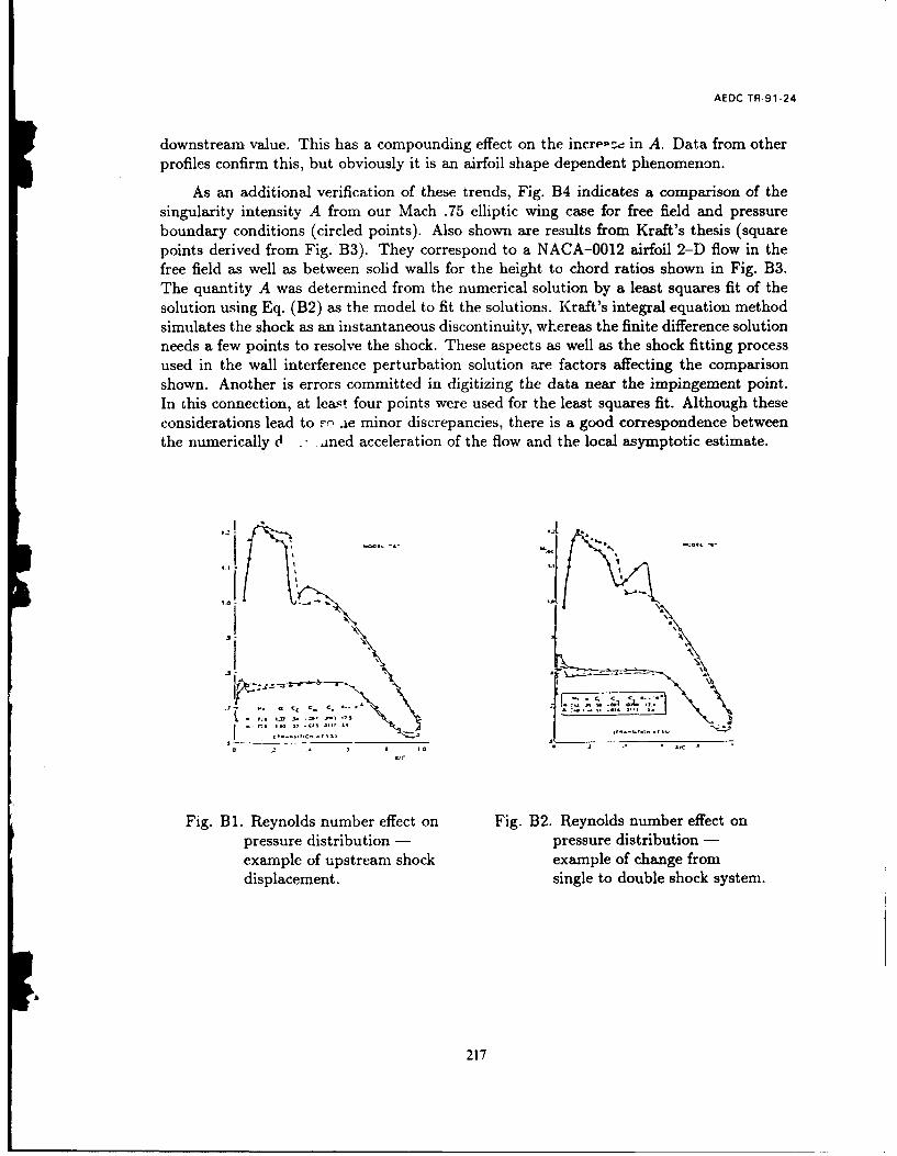
AEDC-TR-91-24
downstream value. This has a compounding effect on the increse in A. Data from otherprofiles confirm this, but obviously it is an airfoil shape dependent phenomenon.
As an additional verification of these trends, Fig. B4 indicates a comparison of thesingularity intensity A from our Mach .75 elliptic wing case for free field and pressureboundary conditions (circled points). Also shown axe results from Kraft's thesis (squarepoints derived from Fig. B3). They correspond to a NACA-0012 airfoil 2-D flow in thefree field as well as between solid walls for the height to chord ratios shown in Fig. B3.The quantity A was determined from the numerical solution by a least squares fit of thesolution using Eq. (B2) as the model to fit the solutions. Kraft's integral equation methodsimulates the shock as an instantaneous discontinuity, wlereas the finite difference solutionneeds a few points to resolve the shock. These aspects as well as the shock fitting processused in the wall interference perturbation solution are factors affecting the comparisonshown. Another is errors committed in digitizing the data near the impingement point.In this connection, at least four points were used for the least squares fit. Although theseconsiderations lead to F9 .ie minor discrepancies, there is a good correspondence betweenthe numerically d .ned acceleration of the flow and the local asymptotic estimate.
0 - -. . I
Fig. B1. Reynolds number effect on Fig. B2. Reynolds number effect onpressure distribution - pressure distribution -example of upstream shock example of change fromdisplacement. single to double shock system.
217

AEOC-TR-91-24
0.9-- . I SOLID EXACT
C-. - 0.8 1 CtRCLIS MALMUTH ET AL
- i j SQUARES KRAFT THESISI0.7
-c.a C0.6
-0 , ,
° 1
a - .' .2-
o~z E ,, ,,0..)
G. I
3,0 . a0 ,-73 C 0. 1 0.2 0.3 0 ,4. 0.5 0 6 0 7 0.3-. -i 22! %0 7 0.3 0.8
o.z a .' a o.e .o 8 F ,,,o 61/3-AEXACTi 7r ,/-b
Fig. B3. Effect of a closed wind tunnel Fig. B4. Comparison of analytical reexpansion
on the pressure distribution singularity with that from numerical
over an NACA-0012 airfoil, solutions.
218