Supplementary Information SUPPLEMENTARY …staff.ulsu.ru/moliver/ref/graphene/nair12.pdfSupplementary Information ... R. R. Nair et al. ... between 350 and 400 keV and current densities

© 2012 Macmillan Publishers Limited. All rights reserved.

SUPPLEMENTARY INFORMATIONDOI: 10.1038/NPHYS2183

NATURE PHYSICS | www.nature.com/naturephysics 1

1

Supplementary Information

Spin-half paramagnetism in graphene induced by point defects

R. R. Nair et al.

#1 Quantitative analysis of fluorination of graphene laminates

Fluorination of graphene laminates was studied using different characterisation techniques such as

Raman spectroscopy, X-ray photoelectron spectroscopy (XPS), and energy dispersive X-ray

microanalysis (EDX). Raman spectroscopy provided a quick qualitative analysis of different levels

of fluorination. This showed that the evolution of Raman spectra of graphene paper with

fluorination (not shown) was very similar to the previously reported spectra for mechanically

exfoliated single layer graphene [S1]. For quantitative determination of the fluorine-to-carbon ratio

(F/C) after different fluorination times we employed XPS. Furthermore, the XPS results for several

samples were corroborated by EDX.

Figure S1. Typical examples of XPS spectra for pristine (bottom curve) and fluorinated (middle and top curves) graphene laminates at different degrees of fluorination.


2

XPS spectra were acquired on a Kratos Axis Ultra X-ray photoelectron spectrometer equipped with

a monochromatic aluminium X-ray source and a delay line detector. Typical wide scan spectra

were recorded from a 220 µm diameter area for binding energies between 0 and 1100eV with a

0.8eV step, at 160eV pass energy. High resolution spectra of C1s and F1s peaks (such as those in

Fig. S1) were recorded with a 0.1eV step, at 40 eV pass energy.

Figure S1 shows typical XPS spectra for energies corresponding to C1s peaks of carbon (left part)

and F1s peaks of fluorine (right part). The three C1s peaks indicate the presence of different types

of carbon bonds while the strong F1s peak appearing after fluorination indicates the presence of

chemisorbed fluorine. An intense peak at ≈ 284eV in the spectrum of pristine graphene paper is due

to the C-C sp2 bonds in graphene [S1]. After exposure of graphene laminates to fluorine the

intensity of this peak decreases while new peaks appear, corresponding to different types of C-F

bonding. The intensities of these new peaks vary for different degrees of fluorination. The most

pronounced peak at ≈289eV, in conjunction with the strong fluorine peak at ≈688eV, yield strong

C-F covalent bonding [S2]. As Fig. S1 shows, the ≈688eV peak is absent for pristine graphene

laminates but shows strongly for all fluorinated samples, which again confirms the presence of

covalently bonded fluorine. The other two peaks at ≈286.3eVand 291eV indicate the presence of C-

CF and CF2 bonds, respectively [S1, S3]. CF2 and CF3 bonds are expected to form primarily at

defects or edges of graphene flakes. Note that the absence of CF3 peaks (≈ 293eV) and very small

intensity of the CF2 peaks indicates that fluorination in our samples occurs mainly at graphene

surfaces, rather than at the defect sites or edges. As all graphene crystallites in the laminates are

very small (typically 30-50 nm), bi- and trilayer graphene flakes (that are present in our laminates

along with 50% monolayers) are easily intercalated by F atoms.

The stoichiometric composition of different fluorinated samples was obtained by analysing the

intensity of carbon and fluorine peaks using Casca XPS software [S4]. Spectra were taken from

several ≈100 m spots on each sample and the results averaged to obtain F/C for a particular

fluorinated sample. This procedure indicated good spatial homogeneity of fluorination on a scale

»100 m, as the calculated F/C ratios varied by no more than 5%. In addition, we carried out EDX

analysis of several fluorinated samples, to confirm the stoichiometry, and found that the results

were in full agreement with the XPS analysis above. These showed that for the longest fluorination

time (80h) we were able to achieve F/C ≈1, i.e. stoichiometric fluorographene. EDX analysis was

also used to confirm that our fluorinated samples were free from contamination with metal

impurities.


3

#2 Irradiation of graphene laminates with high-energy ions

For C4+ irradiations we used 5MV van de Graaf tandem accelerator where samples, mounted on

aluminium foil, were clamped to a copper rod cooled with liquid nitrogen to -50°C. The sample

temperature, which was monitored using an infrared temperature sensor, remained below 50°C

during irradiation and the vacuum was maintained in the 10-6-10-7 mbar range. To ensure irradiation

homogeneity, the focused beam spot was rasterized over the sample area using two perpendicular

electromagnets. The fluence was determined from the total charge accumulated in the target

chamber.

Proton irradiations were carried out in a 500kV ion implanter, at room temperature and energies

between 350 and 400 keV and current densities <0.2 µA/cm2. Two perpendicular electric fields

were used to sweep the beam over the sample area and the radiation fluence was measured using

four Faraday cups with a known window area. No considerable heating of the target is expected

with the used energies and currents. The concentration of backscattered protons which stopped in

the sample is estimated to be less than 1 ppm.

The fluences used to achieve the defect densities in Fig. 4 of the main text varied from 5·1013 to

1·1016 cm-2. We note that it was not possible to derive the defect density for each sample from the

fluence alone, because different samples had different surface areas and different defect

distributions. The defect densities shown in Fig. 4 (main text) were calculated for each sample on

the basis of the corresponding fluence, surface area and the number of vacancies created by each

type of ions as obtained from SRIM simulations.

To check for the possibility of vacancy-interstitial recombination during or after irradiation [S5],

one of the proton-irradiated samples was annealed at 300°C for 8h, which resulted in ~20%

reduction in magnetic moment. This shows that the majority of vacancies in our samples do not

recombine even at temperatures much higher than room temperature, in agreement with the higher

mobility of interstitials in few-layer graphene compared to graphite [S6].

#3 Determination of the spin value from magnetisation data

To characterize the magnetic species contributing to the magnetization M of fluorinated and

irradiated graphene laminates, we plotted M as a function of the reduced field H/T. For all samples

(i.e. all degrees of fluorination and all vacancy concentrations) M(H/T) curves measured at

different temperatures collapse on a single curve, indicating that graphene with both types of

defects behaves as a paramagnet with a single type of non-interacting spins. As an example, Fig.


4

S2(a) shows such analysis for the fully fluorinated graphene (x =1). The observed behavior is

accurately described by the Brillouin function, such that the initial slope of M(H/T) is determined

by the angular momentum quantum number J and the g factor, and the saturation level is

determined by the number of magnetic moments (spins) N:

J

x

JJ

xJ

J

JNgJM B 2

ctnh2

1

2

12ctnh

2

12

where TkHgJx BB /μ and kB the Boltzmann constant. Assuming g=2 (there are no indications in

literature that g-factor in graphene may be enhanced), the Brillouin function provides excellent fits

to the data for J =S=1/2 (red curve Fig. S2(a)). For comparison, we also show fitting curves for J =1,

3/2 and 2, all of which provide very poor fits, making it clear that only J = S =1/2 fits the data.

Figure S2. Determination of the angular momentum quantum number J from ∆M vs H/T curves. (a) Magnetisation of the fully fluorinated graphene crystallites, x=1 (linear diamagnetic background subtracted). Symbols are data for three different temperatures and solid curves are fits to the Brillouin function for J =1/2, 1, 3/2 and 2. (b) Magnetisation due to vacancies: As the increase in M after irradiation was comparable to the paramagnetic signal in pristine graphene, ∆M here is the magnetisation over and above the paramagnetic contribution measured before irradiation (linear diamagnetic background subtracted as well). Grey symbols show data for two different vacancy concentrations (lower curve 2.4·1019 g-1, upper curve 7.4·1019 g-1) and solid lines show Brillouin function fits with g=2 and J =1/2, 1, 3/2 and 2.

Figure S2(b) shows similar analysis for two different vacancy concentrations in graphene laminates

irradiated with 350 keV protons. Again, only J=S=1/2 fits the data, with all other values of J giving

very poor fits. This provides the most unequivocal proof that both types of point defects studied -

fluorine adatoms and vacancies - represent non-interacting paramagnetic centers with spin S=1/2.


5

#4 Commentary on ferromagnetism reported for HOPG

Weak ferromagnetic signals (10-3 emu/g) were found in pristine highly-oriented pyrolytic graphite

(HOPG) (e.g. [S7,S8]) which, according to the authors, could not be explained by 1-2ppm of Fe

detected using particle-induced X-ray emission (PIXE) or X-ray fluorescence spectroscopy

(XRFS). Accordingly, the ferromagnetism was attributed to intrinsic defects, such as, e.g., grain

boundaries [S8]. The ferromagnetic response was shown to increase dramatically after high-energy

ion irradiation of HOPG [S9-S13], nanodiamonds [S14], carbon nanofoams [S15] and carbon films

[S16]. Several scenarios have been suggested to explain the observed ferromagnetism.

Trying to clarify the situation, we have carried out extensive studies of magnetic behaviour of

HOPG crystals obtained from different manufacturers (ZYA-, ZYB-, and ZYH-grade from NT-

MDT and SPI-2 and SPI-3 from SPI Supplies). These crystals are commonly used for studies of

magnetism in graphite; e.g., ZYA-grade crystals were used in refs. S7, S9-S13 and ZYH-grade in

ref. S8. We have also observed weak ferromagnetism, similar in value to the one reported

previously for pristine (non-irradiated) HOPG. Below, we show that the ferromagnetism in ZYA-,

ZYB-, and ZYH-grade crystals is due to micron-sized magnetic inclusions (containing mostly Fe),

which can easily be visualized by scanning electron microscopy (SEM) in the backscattering mode.

Without the intentional use of this technique, the inclusions are easy to overlook. No such

inclusions were found in SPI crystals and, accordingly, in our experiments these crystals were

purely diamagnetic at all temperatures (no ferromagnetic signals at a level of 10-5 emu/g).

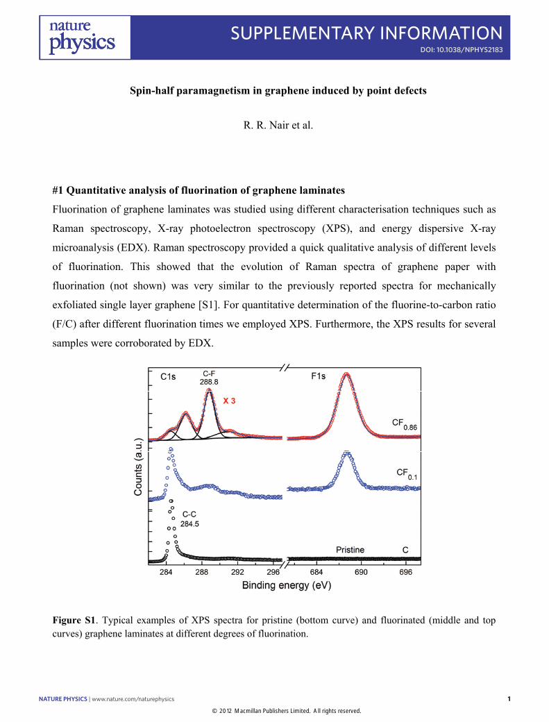
Figure S3. Ferromagnetic response in different HOPG crystals. Magnetic moment ∆M vs applied field H after subtraction of the linear diamagnetic background. The inset shows a low-field zoom of three curves from the main panel where the remnant ∆M and coercive force are seen clearly.


6

Ten HOPG crystals of different grades (ZYA, ZYB, ZYH and SPI) were studied using SQUID

magnetometry (Quantum Design MPMS XL7), XRFS, SEM and chemical microanalysis by means

of energy-dispersive X-ray spectroscopy (EDX). For all ZYA, ZYB and ZYH crystals, magnetic

moment vs field curves, M(H), showed characteristic ferromagnetic hysteresis in fields below 2000

Oe, which was temperature independent between 2K and room T, implying a Curie temperature

significantly above 300K. The saturation magnetisation MS varied from sample to sample by more

than 10 times, from 1.2·10-4emu/g to 3·10-3 emu/g – see Fig. S3. This is despite the fact that XRFS

did not detect magnetic impurities in any of our HOPG crystals (with a detection limit better than a

few ppm). This result is similar to the findings of other groups [e.g. S9, S10, S11, S16]. Figure S3

also shows an M(H) curve for one of the SPI crystals, where no ferromagnetism could be detected.

The seemingly random values of ferromagnetic signal in nominally identical crystals could be an

indication that the observed ferromagnetism is related to structural features of HOPG, such as grain

boundaries, as suggested in ref. [S8]. However, we did not find any correlation between the size of

the crystallites making up HOPG crystals and/or their misalignment and the observed MS. For

example, the largest MS as well as the largest coercive force, MC, were found for one of the ZYA

crystals, which have the smallest mosaic spread (0.4-0.7), and for a ZYH crystal with the largest

mosaic spread (3-5). Furthermore, crystallite sizes were rather similar for all ZYA, ZYB and ZYH

crystals (see Fig. S4) while MS varied by almost a factor of 3 (see Fig. S3).

Figure S4. Typical, same-scale, SEM images of crystallites in different HOPG samples: (a) ZYH; (b) ZYA; (c) SPI. Typical crystallite sizes in ZYH, ZYB and ZYA are 2 to 5 µm; in SPI crystallites vary from 0.5 to

15 µm. The scale bar corresponds to 5m.

To investigate whether the observed ferromagnetism is homogeneous within the same

commercially available 1cm1cm0.2cm HOPG crystal, we measured magnetisation of four

samples cut out from the same ZYH crystal as shown in the inset of Fig. S5. To exclude possible

contamination of the samples due to exposure to ambient conditions, both exposed surfaces were

cleaved and the edges cut off just before the measurements. Surprisingly, we found significant

variations of the ferromagnetic signal between these four nominally identical samples – see Fig. S5.


7

This indicates that the observed ferromagnetism is not related to structural or other intrinsic

characteristics of HOPG crystals, as these are the same for a given crystal. Therefore, it seems

reasonable to associate the magnetic response with external factors, such as, for example, the

presence of small inclusions of another material.

Figure S5. Ferromagnetic hysteresis in four samples cut from the same ZYH HOPG crystal. The inset shows schematically positions of the samples in the original crystal.

To check this hypothesis, we examined samples of different HOPG grades using backscattering

SEM. Due to its sensitivity to the atomic number [S17], backscattered electrons can provide a

strong contrast allowing to detect particles made of heavy elements inside a light matrix (graphite

in our case). This experiment revealed that all ZYA, ZYB, and ZYH crystals contained sparsely

distributed micron-sized particles of a large atomic number, with typical in-plane separations of 100

to 200 m – see Fig. S6(a). Comparison of SEM images in backscattering and secondary electron

modes (BS and SE, respectively) revealed that in most cases the particles were buried under the

surface of the sample and, therefore, were not visible in the most commonly used secondary

electron mode. This is illustrated in Fig. S6(b) which shows the same area of a ZYB sample in the

SE and BS modes. The difference between the two images is due to different energies and

penetration depths for secondary and backscattered electrons: The energy of BS electrons is close to

the primary energy, i.e. 20 keV in our case, and they probe up to 1m thick layer at the surface

[S17] while secondary electrons have characteristic energies of the order of 50 eV and come from a

thin surface layer of a nm thickness [S18]. Importantly, no such inclusions could be detected in SPI

samples that, as discussed, did not show any ferromagnetic response. The difference between ZY

and SPI grades is presumably due to different manufacturing procedures used by different


8

suppliers. Our attempts through NT-MDT to find out the exact procedures used for production of

ZY grades of HOPG were unsuccessful.

Figure S6. (a) SEM images of ZYA (top) and ZYH (bottom) samples in back-scattering mode. Small white particles are clearly visible in both images, with typical separations between the particles of 100 µm for ZYA and 240 µm for ZYH. Insets show zoomed-up images of the particles indicated by arrows; both particles are ≈2µm in diameter. (b) SEM images of the same particle found in a ZYB sample taken in backscattering (top) and secondary electron (bottom) modes. Surface features are clearly visible in the SE image while BS is mostly sensitive to chemical composition. The contrast around the particle in the SE mode is presumably due to a raised surface in this place.

To analyse the chemical composition of the detected particles we employed in situ energy-

dispersive X-ray spectroscopy (EDX) that allows local chemical analysis within a few m3 volume.

Figure S7 shows a typical EDX spectrum collected from a small volume (so-called interaction

volume) around a 2.5 m diameter particle in a ZYA sample. This particular spectrum corresponds

to the presence of 8.6 wt% (2.1 at%) Fe, 2.3 wt% (0.65%) Ti, 1.8 wt% V (0.47 at%) and <0.5 wt%

Ni, Cr and Co, as well as some oxygen, which appear on top of 86 wt% (96.5 at%) of carbon. The

latter contribution is attributed to the surrounding graphite within the interaction volume. To

determine the actual composition of the inclusion, we needed to take into account that the above

elemental analysis applies to the whole interaction volume, where the primary electrons penetrate

into the sample. Given that 96% of the interaction volume is made up by carbon, the electron range

R and, accordingly, the interaction volume can be estimated to a good approximation using the

Kanaya-Okayama formula [S19]:


9

μm5.489.0

67.10276.0

Z

EAR ,

where A=12 g/mole is the atomic weight of carbon, E=20 keV the beam energy, Z=6 the atomic

number and ρ=2.25 g/cm3 the density of graphite. Using the calculated value of R, the weight

percentages for different elements from the spectrum and their known densities, it is

straightforward to show that the volume occupied by the detected amount of Fe and Ti is in

excellent agreement with the dimensions of the particle in Fig. S7, i.e., the particle is made up

predominantly of these two elements. The presence of oxygen indicates that Fe and Ti are likely to

be in an oxidised state, i.e. the particle is either magnetite or possibly titanomagnetite, both of

which are ferrimagnetic, with saturation magnetisation MS ≈ 75-90emu/g [S20].

Figure S7. EDX spectrum of one of the particles found in a ZYA sample. Inset shows SEM image of the particle.

We estimate that a 2.5µm diameter particle of magnetite contributes ≈2.5·10-9 emu to the overall

magnetisation. Therefore, the observed ferromagnetic signal (1.5·10-5 emu) for this particular ZYA

sample (330.26 mm) implies that the sample contains 6,000 magnetite particles which, if

uniformly distributed, should be spaced by 100 µm in the ab plane. This is in agreement with our

SEM observations. This allows us to conclude that the visualized magnetic particles can indeed

account for the whole ferromagnetic signal for this sample.

BS and EDX analysis of the other HOPG samples showing ferromagnetism produced similar

results, with some samples containing predominantly Fe and others both Fe and Ti, as in the

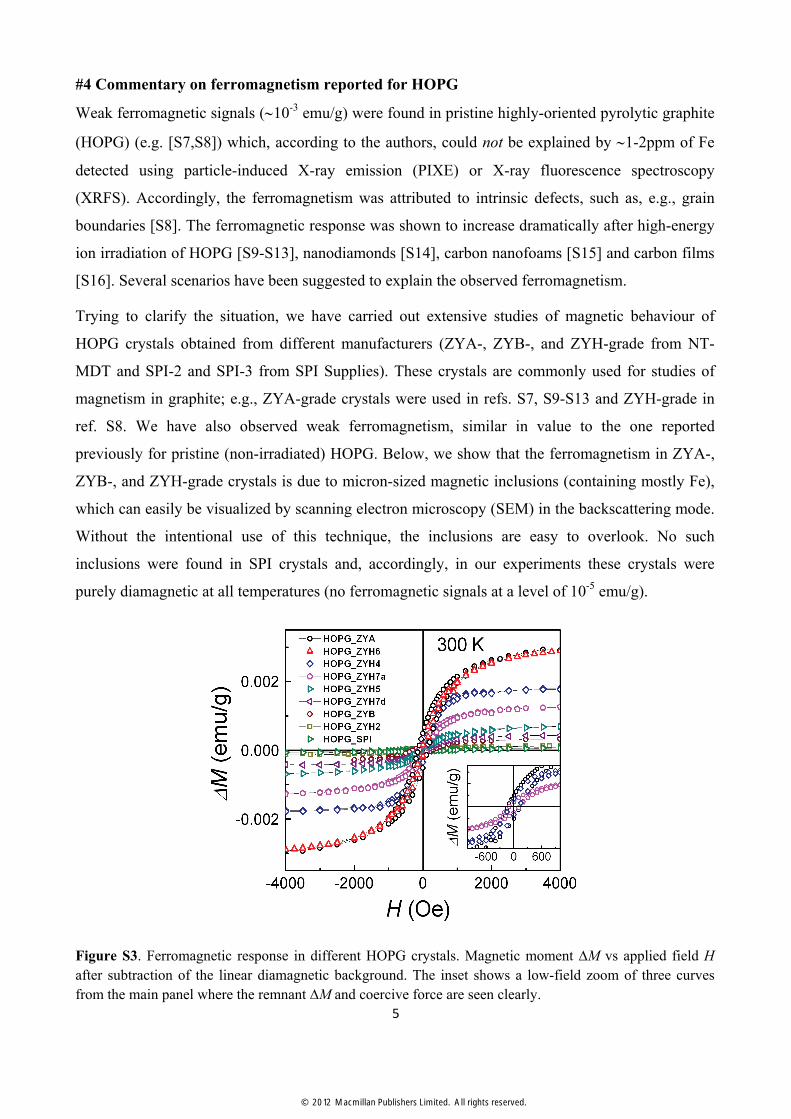
example above. A clear correlation has been found between the value of MS for a particular sample

and the average separation of the magnetic particles detected by BS/EDX – see Fig. S8. No


10

magnetic particles could be found in SPI samples and, accordingly, they did not show any

ferromagnetic signal.

Figure S8. Saturation magnetisation Ms as a function of the inverse of the average separation between the detected particles d as determined from the backscattering images (see text).

On the basis of the above analysis, we conclude that ferromagnetism in our ZYA, ZYB and ZYH

HOPG samples is not intrinsic but due to contamination with micron-sized particles of probably

either magnetite or titanomagnetite. As these particles were usually detected at submicron distances

below the sample surface (see above), they should have been introduced during high-temperature

crystal growth. We note that ZYA, ZYB or ZYH grades of HOPG are most commonly used for

studies of magnetism in graphite (e.g., ZYA-grade crystals were specified in refs. [S7, S9-S13])

and, therefore, the contamination could be the reason for the often reported ferromagnetism.

Finally, we would like to comment why magnetic particles such as those observed in the BS mode

could have been overlooked by commonly used elemental analysis techniques, such as XRFS and

PIXE [S7-S16]. Assuming that all particles found in our samples are magnetite and of

approximately the same size, 2-3 µm, we estimate that the total number of Fe and Ti atoms in our

samples ranges from 1 to 6 ppm. In the case of XRFS, 5 ppm of Fe is close to its typical detection

limit and these concentrations might remain unnoticed. In the case of PIXE, its resolution is better

than 1ppm. PIXE was used in e.g. refs. [S9, S11] for ZYA graphite, where no contamination was

reported but the saturation magnetisation was ≈ (1-2)·10-3 emu/g, similar to our measurements. The

absence of detectable concentrations of magnetic impurities has been used as an argument that the

ferromagnetic signals could not be due to contamination. Also, it was usually assumed that any

remnant magnetic impurities were distributed homogeneously, rather than as macroscopic particles,


11

and therefore would give rise to paramagnetism rather than a ferromagnetic signal, which was used

as an extra argument against magnetic impurities.

It is clear that the latter assumption is incorrect, at least for the case of ZY grade graphite.

Furthermore, let us note that the difference of several times for the limit put by PIXE and the

amount measured by SQUID magnetometry is not massive. In our opinion, this difference can be

explained by the fact that PIXE tends to underestimate the concentration of magnetic impurities if

they are concentrated into relatively large particles. Indeed, PIXE probes only a thin surface layer

(1µm for 200 keV protons) which is thinner than the diameter of the observed magnetic

inclusions. One can estimate that for round-shape inclusions with diameters of ~3m, there should

be a decrease by a factor of 3 in the PIXE signal with respect to the real concentration. Even more

importantly, inclusions near the surface of HOPG provide weak mechanical points and are likely to

be removed during cleavage when a fresh surface is prepared. Therefore, we believe that a micron-

thick layer near the HOPG surface is unlikely to be representative of the whole sample. In contrast,

magnetisation measurements probe average over the bulk of the samples, which can explain the

observed several times discrepancy.

#5 Remnant ferromagnetism in graphene laminates

Preparation of graphene laminates involves splitting of graphite into individual graphene planes.

Therefore, if standard HOPG ZYH or ZYA crystals are used, one can expect that magnetic particles

present in the starting crystals may in principle pass into graphene laminates, despite the fact that

centrifugation should mostly remove heavy particles from the suspension. Indeed, careful

measurements of sufficiently large samples of graphene laminates made from ZYH-grade HOPG

detected very weak ferromagnetic signals – see Fig. S9. For a typical 1.5-2mg graphene laminate

sample the ferromagnetic component of magnetisation, MS (300K), was found to be <5·10-7 emu.

Therefore, measuring the corresponding hysteresis loops required the maximum possible sensitivity

of our SQUID magnetometer (<1·10-7 emu), which we achieved by using the RSO option and

taking great care in terms of sample mounting and background uniformity. Apart from the smaller

MS, all other characteristics of the ferromagnetic signal in the laminates (temperature independence,

remnant magnetisation and coercive force) were similar to those for the starting HOPG samples,

indicating the same origin of ferromagnetism – see Fig. S9.


12

Figure S9. Comparison of the ferromagnetic magnetisation in HOPG ZYH and a typical sample of graphene laminate

Some samples used in our fluorination and irradiation experiments were additionally purified by

immersion for several hours in a mixture of HNO3 and HF acids and subsequent annealing at

300°C. The above acids are efficient in dissolving metal impurities, either in oxidised or pure metal

form. After such treatment, no ferromagnetism was observed in any of these samples. Similar

treatment of HOPG samples led to a reduction in MS but not complete disappearance of the

ferromagnetic signal. This result is easy to understand, as acids can penetrate between the

decoupled graphene layers in laminate samples relatively easily, and this is not the case for bulk

HOPG.

We conclude that the very weak but still detectable ferromagnetic response that we sometimes

observed in graphene samples prepared from commonly available HOPG crystals also results from

the initial contamination of HOPG, which should be taken into account when studying magnetic

properties of graphene laminates and its derivatives.

Supplementary references

S1. Nair, R. R. et al. Fluorographene: A two-dimensional counterpart of Teflon. Small 6, 2877-2884 (2010).

S2. Touhara, H., Okino F. Property control of carbon materials by fluorination. Carbon 38, 241-267 (2000).

S3. Robinson J. T. et al. Properties of fluorinated graphene films. Nano Letters 10, 3001-3005 (2010).

S4. http://www.casaxps.com/.

S5. Telling R. H., Heggie M. I. Radiation defects in graphite. Phil. Mag. 87, 4796-4846 (2007).


13

S6. Gulans A., Krasheninnikov A. V., Puska M. J., Nieminen R. M. Bound and free self-interstitial defects in graphite and bilayer graphene: A computational study. Phys. Rev. B 84, 024114 (2011).

S7. Esquinazi P., Setzer A., Höhne R., Semmelhack C. Ferromagnetism in oriented graphite samples. Phys. Rev. B 66, 024429 (2002).

S8. Cervenka J., Katsnelson M. I., Flipse C. F. J. Room-temperature ferromagnetism in graphite driven by two-dimensional networks of point defects. Nature Physics 5, 840-844 (2009).

S9. Esquinazi P. et al. Induced magnetic ordering by proton irradiation in graphite, Phys. Rev. Lett. 91, 227201 (2003).

S10. Quiquia B. et al. A comparison of the magnetic properties of proton- and iron-implanted graphite. Eur. Phys. J. B 61, 127-130 (2008).

S11. Makarova T. L., Shelankov A. L., Serenkov I. T., Sakharov V. I., Boukhvalov D. W. Anisotropic magnetism of graphite irradiated with medium-energy hydrogen and helium ions. Phys. Rev. B 83, 085417 (2011).

S12. He Z. et al. Raman study of correlation between defects and ferromagnetism in graphite. J. Phys. D: Appl. Phys. 44, 085001 (2011).

S13. Ramos M. A. et al. Magnetic properties of graphite irradiated with MeV ions. Phys. Rev. B 81, 214404 (2010).

S14. Talapatra S. et al. Irradiation-induced magnetism in carbon nanostructures. Phys. Rev. Lett. 95, 097201 (2005).

S15. Rode A. V. et al. Unconventional magnetism in all-carbon nanofoam. Phys. Rev. B 70, 054407 (2004).

S16. Ohldag H. et al. π-Electron ferromagnetism in metal-free carbon probed by soft X-ray dichroism. Phys. Rev. Lett. 98, 187204 (2007).

S17. Murata K. Exit angle dependence of penetration depth of backscattered electrons in the scanning electron microscope. Phys. Stat. Sol. (a) 36, 197-208 (1976).

S18. Eberhart J. P. Structural and Chemical Analysis of Materials (John Wiley & Sons, 1991)

S19. Kanaya K., Okayama S. Penetration and energy-loss theory of electrons in solid targets. J. Phys. D: Appl. Phys. 5, 43-58 (1972).

S20. Goss C. J. Saturation magnetisation, coercivity and lattice parameter changes in the system Fe3O4-γFe2O3, and their relationship to structure. Phys. Chem. Minerals 16, 164-171(1988).

Documents

Supplementary Information SUPPLEMENTARY …staff.ulsu.ru/moliver/ref/graphene/nair12.pdfSupplementary Information ... R. R. Nair et al. ... between 350 and 400 keV and current densities