Pennsylvania Society of Land Surveyors

The Why’s, How’s, and Best Practices in Performing a

Localization/Site Calibration of a GNSS Survey

Dr. Charles Ghilani

Class Etiquette

• Turn off all cell phones

– Or set them to vibrate

– Answer all calls outside the room

• Ask questions at any point during the class.

– Simply speak up so that all can hear your question

2

Overview

• This workshop will cover

– The various coordinate reference frames that surveyors may run into in

practice today such as NAD83 (2011), (2007), NAD83 (CORS96), …, and

WGS84 (G1762), (G1674), (G1150), ... and so on

– Discuss the best practices in performing a localization/site calibration to

place your GNSS receiver in the proper reference frame

– Discuss software available from the NGS to transfer coordinates from

various historical reference frames into NAD83 (2011) or vice versa

– Discuss the mathematics and implications that can occur when best

practices are not followed

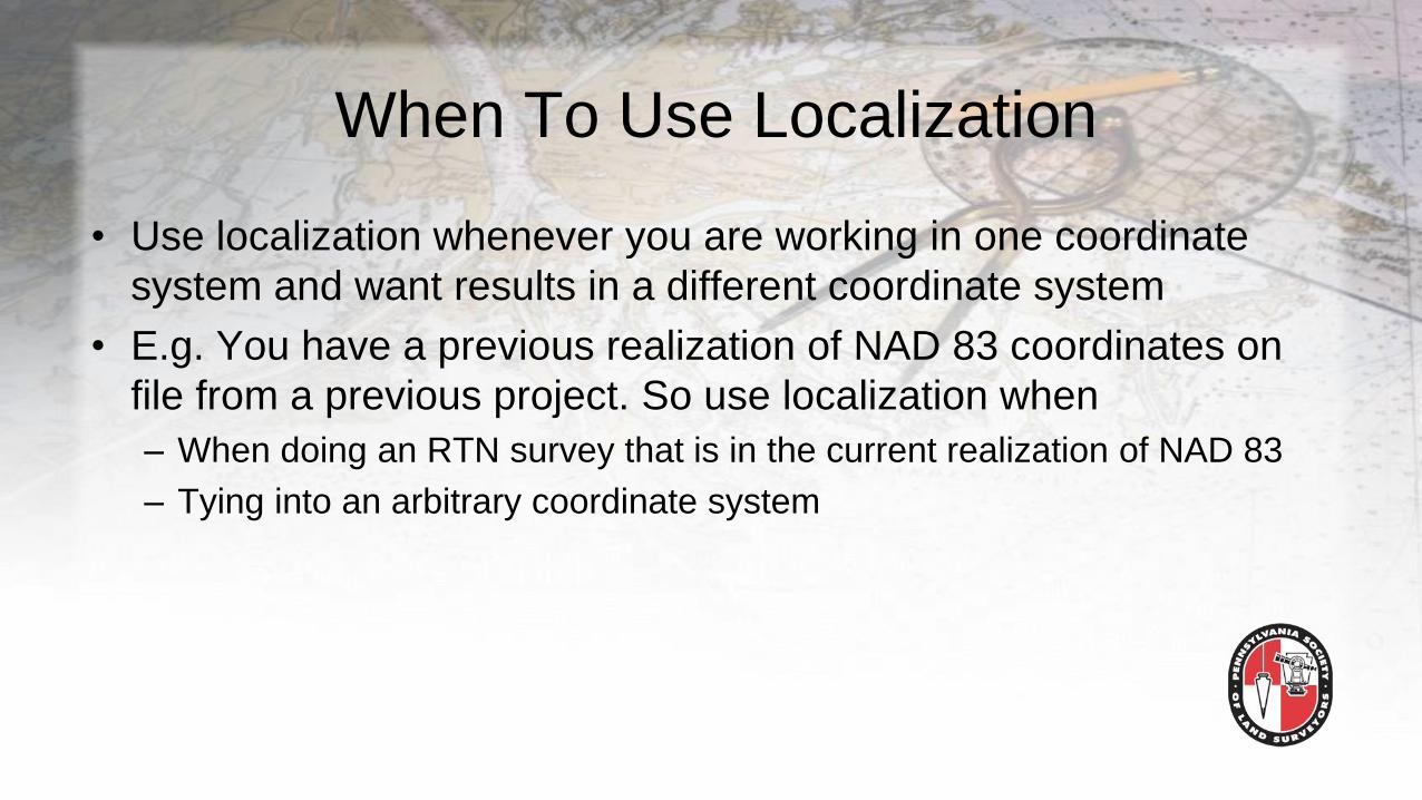
When To Use Localization

• Use localization whenever you are working in one coordinate

system and want results in a different coordinate system

• E.g. You have a previous realization of NAD 83 coordinates on

file from a previous project. So use localization when

– When doing an RTN survey that is in the current realization of NAD 83

– Tying into an arbitrary coordinate system

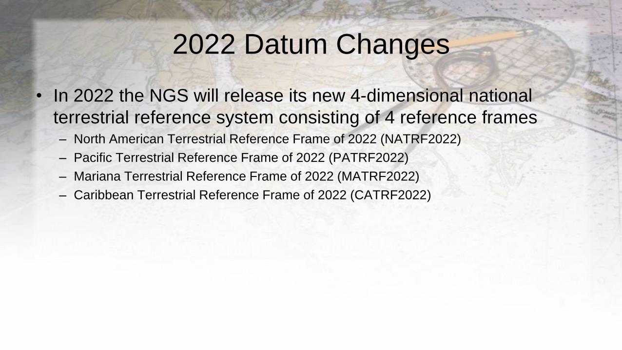
2022 Datum Changes

• In 2022 the NGS will release its new 4-dimensional national

terrestrial reference system consisting of 4 reference frames– North American Terrestrial Reference Frame of 2022 (NATRF2022)

– Pacific Terrestrial Reference Frame of 2022 (PATRF2022)

– Mariana Terrestrial Reference Frame of 2022 (MATRF2022)

– Caribbean Terrestrial Reference Frame of 2022 (CATRF2022)

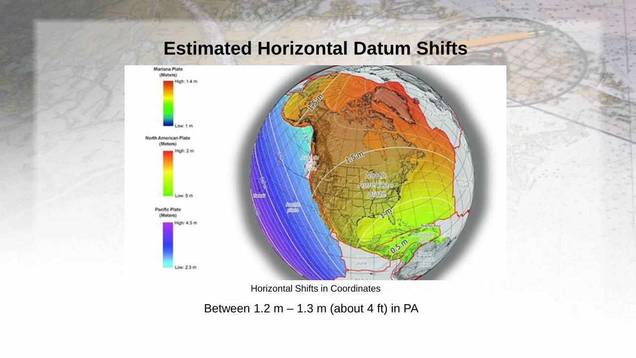
Estimated Horizontal Datum Shifts

Horizontal Shifts in Coordinates

Between 1.2 m – 1.3 m (about 4 ft) in PA

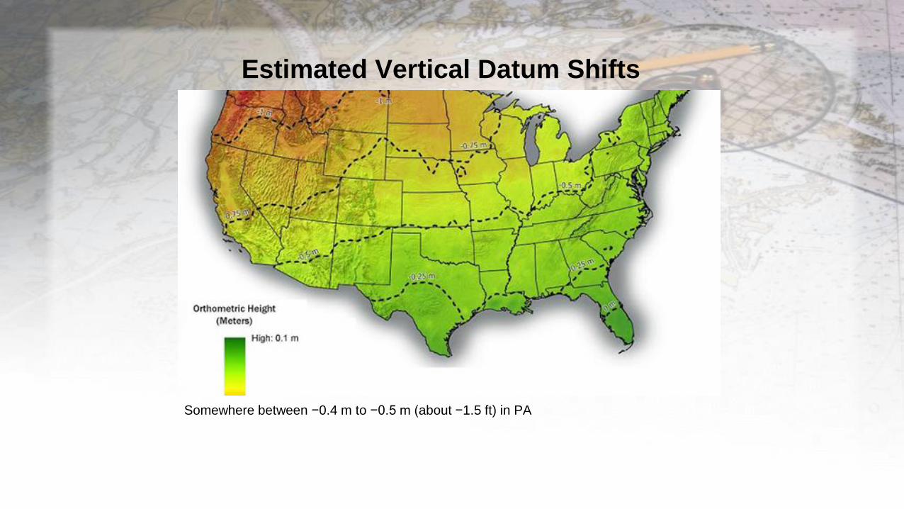
Estimated Vertical Datum Shifts

Somewhere between −0.4 m to −0.5 m (about −1.5 ft) in PA

When to Use Localization

• If you plan on using coordinates of locations determined

in a prior datum, you can either:

1. Perform a localization on points and place your previous work

into the 2022 datum or vice versa

2. Use NGS supplied transformations to transform prior

coordinates into the new datum

• Will not be as accurate as 1.

Real Scenario from

a previous change in realizations of NAD 83

• Company performs a survey for a client in 2011. In the

process it creates control monumentation using an RTN-

GNSS receiver for later engineering design work.

– In July of 2012 they return to do a site survey for a new building

in the same location

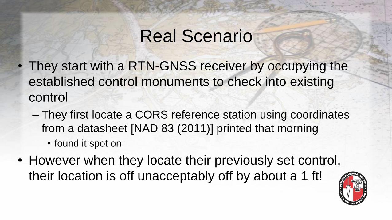
Real Scenario

• They start with a RTN-GNSS receiver by occupying the

established control monuments to check into existing

control

– They first locate a CORS reference station using coordinates

from a datasheet [NAD 83 (2011)] printed that morning

• found it spot on

• However when they locate their previously set control,

their location is off unacceptably off by about a 1 ft!

Real Scenario

• Put the GNSS receiver back in the truck

– Perform site survey with total station by occupying previously

established control

– What should have been a few-hour survey was now an all-day

optical survey

Problem

• Why didn’t their control agree with their RTN-GNSS

receiver coordinates?

– Previously set control had NAD 83 (2007) coordinates

• NGS and RTN changed to NAD83 (2011) on June 30, 2012

– Their RTN defaulted to the newer NAD 83 (2011) coordinates

– This problem will become apparent when NGS releases its new

datum in 2022

Solutions

• They could have:

1. Converted the NAD 83 (2007) coordinates to NAD 83 (2011)

before coming to the field

2. Localized their survey to NAD 83 (2007) coordinates

3. Used a single-base RTK survey with base station coordinates

that match previous survey

4. Changed the default datum to NAD83 (2007) in controller

λ

Z Axis

X Axis

Y Axis

f(φ,λ,h) = (X,Y,Z)

hEarth’s

Surface

Zero

Meridian

Mean Equatorial Plane

Reference Ellipsoid

P

GNSS-Derived Coordinates

Geoid

H

Mass

center

CTP

h = H + N f(φ,λ) = (N,E)

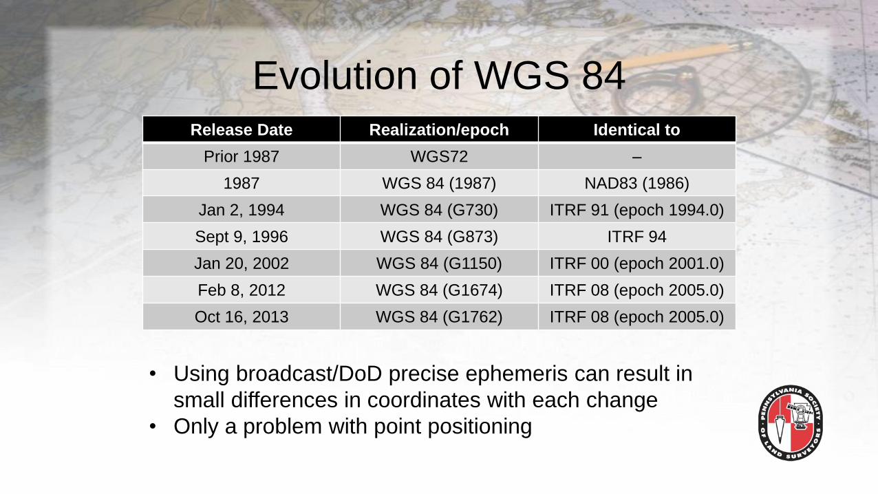
Evolution of WGS 84Release Date Realization/epoch Identical to

Prior 1987 WGS72 –

1987 WGS 84 (1987) NAD83 (1986)

Jan 2, 1994 WGS 84 (G730) ITRF 91 (epoch 1994.0)

Sept 9, 1996 WGS 84 (G873) ITRF 94

Jan 20, 2002 WGS 84 (G1150) ITRF 00 (epoch 2001.0)

Feb 8, 2012 WGS 84 (G1674) ITRF 08 (epoch 2005.0)

Oct 16, 2013 WGS 84 (G1762) ITRF 08 (epoch 2005.0)

• Using broadcast/DoD precise ephemeris can result in

small differences in coordinates with each change

• Only a problem with point positioning

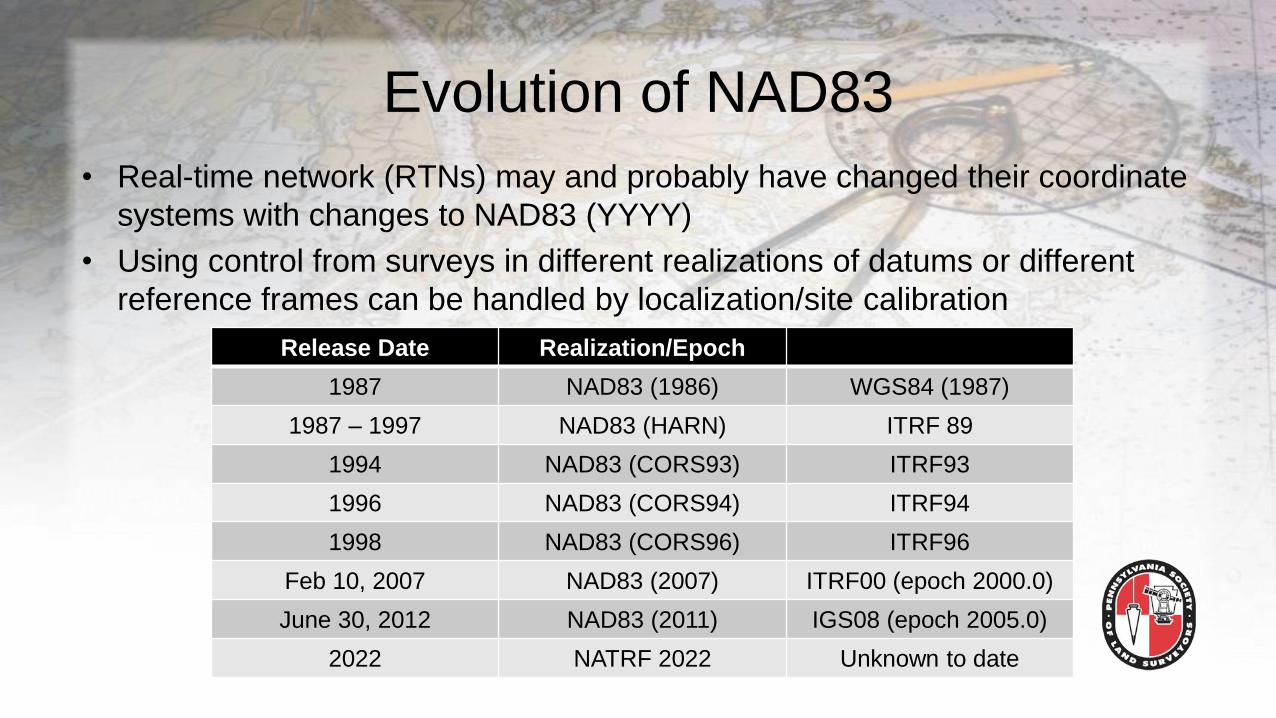
Evolution of NAD83

• Real-time network (RTNs) may and probably have changed their coordinate

systems with changes to NAD83 (YYYY)

• Using control from surveys in different realizations of datums or different

reference frames can be handled by localization/site calibration

Release Date Realization/Epoch

1987 NAD83 (1986) WGS84 (1987)

1987 – 1997 NAD83 (HARN) ITRF 89

1994 NAD83 (CORS93) ITRF93

1996 NAD83 (CORS94) ITRF94

1998 NAD83 (CORS96) ITRF96

Feb 10, 2007 NAD83 (2007) ITRF00 (epoch 2000.0)

June 30, 2012 NAD83 (2011) IGS08 (epoch 2005.0)

2022 NATRF 2022 Unknown to date

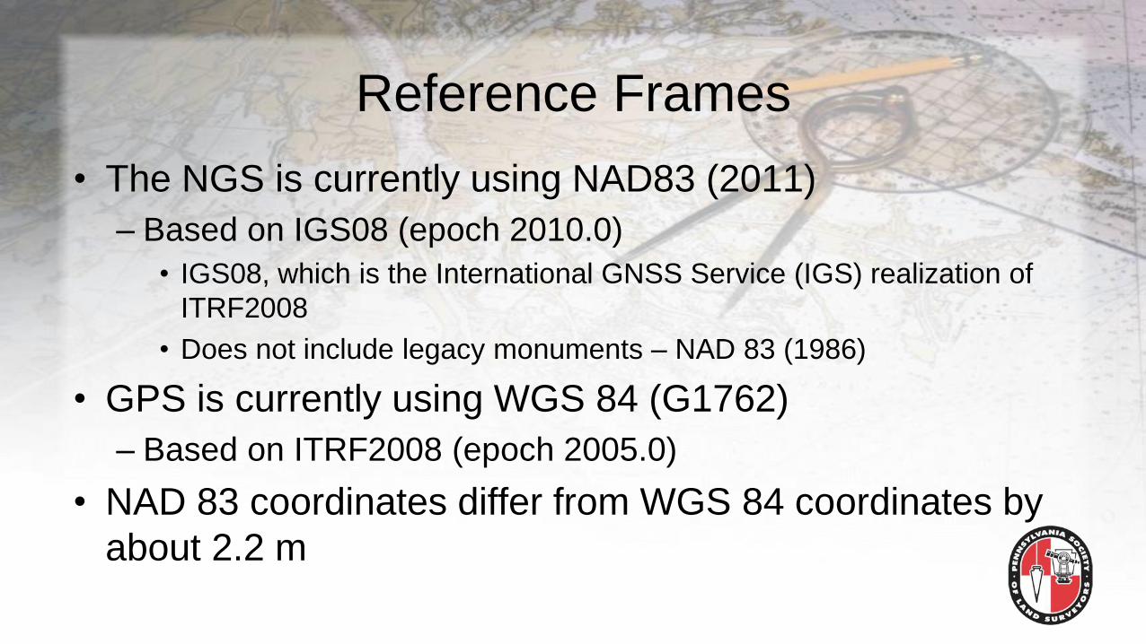
Reference Frames

• The NGS is currently using NAD83 (2011)

– Based on IGS08 (epoch 2010.0)

• IGS08, which is the International GNSS Service (IGS) realization of

ITRF2008

• Does not include legacy monuments – NAD 83 (1986)

• GPS is currently using WGS 84 (G1762)

– Based on ITRF2008 (epoch 2005.0)

• NAD 83 coordinates differ from WGS 84 coordinates by

about 2.2 m

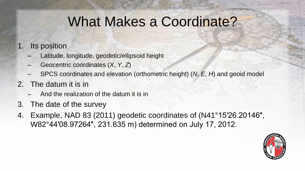
What Makes a Coordinate?

1. Its position

– Latitude, longitude, geodetic/ellipsoid height

– Geocentric coordinates (X, Y, Z)

– SPCS coordinates and elevation (orthometric height) (N, E, H) and geoid model

2. The datum it is in

– And the realization of the datum it is in

3. The date of the survey

4. Example, NAD 83 (2011) geodetic coordinates of (N41°15′26.20146″,

W82°44′08.97264″, 231.635 m) determined on July 17, 2012.

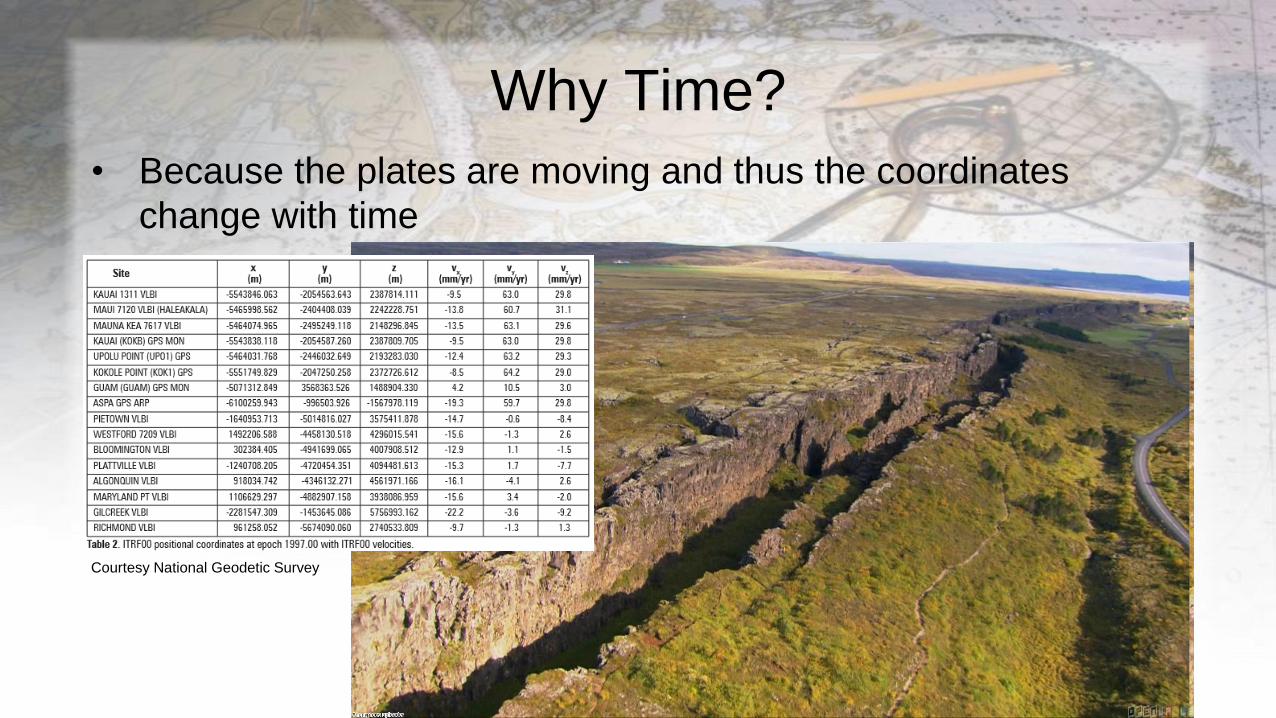
Why Time?

• Because the plates are moving and thus the coordinates

change with time

Courtesy National Geodetic Survey

What Makes a Coordinate?

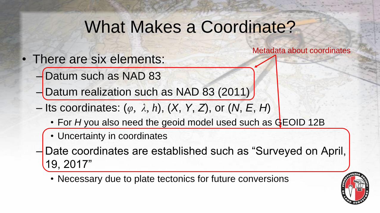
• There are six elements:

– Datum such as NAD 83

– Datum realization such as NAD 83 (2011)

– Its coordinates: (φ, λ, h), (X, Y, Z), or (N, E, H)

• For H you also need the geoid model used such as GEOID 12B

• Uncertainty in coordinates

– Date coordinates are established such as “Surveyed on April,

19, 2017”

• Necessary due to plate tectonics for future conversions

Metadata about coordinates

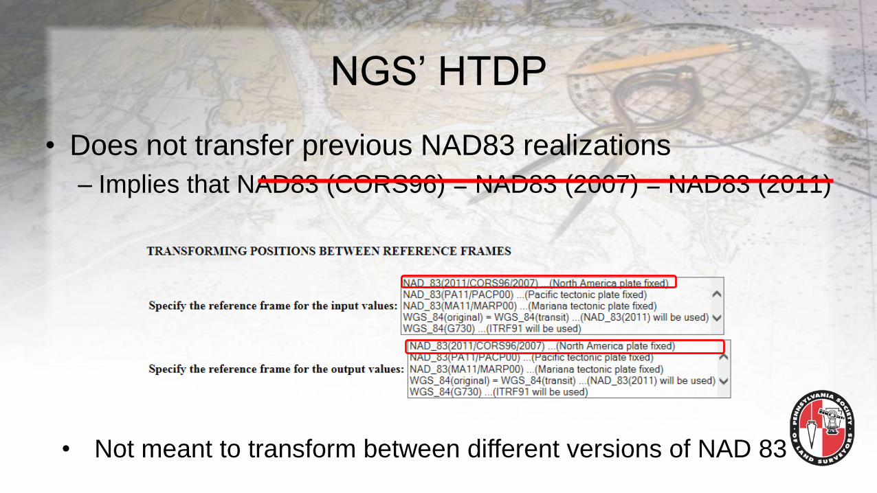
NGS’ HTDP

• Does not transfer previous NAD83 realizations

– Implies that NAD83 (CORS96) = NAD83 (2007) = NAD83 (2011)

• Not meant to transform between different versions of NAD 83

Converting NAD83 (2007) to (2011)

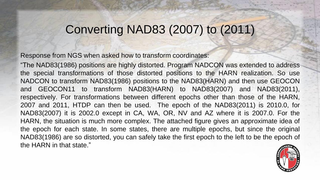
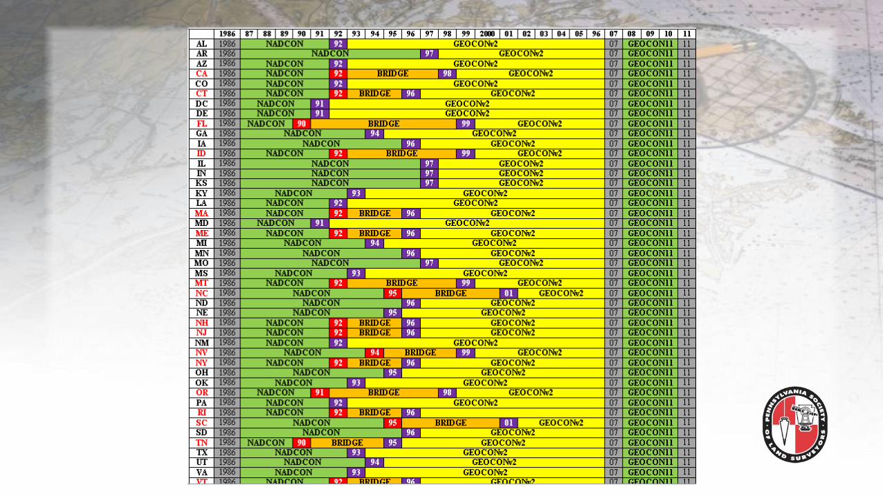
Response from NGS when asked how to transform coordinates:

“The NAD83(1986) positions are highly distorted. Program NADCON was extended to address

the special transformations of those distorted positions to the HARN realization. So use

NADCON to transform NAD83(1986) positions to the NAD83(HARN) and then use GEOCON

and GEOCON11 to transform NAD83(HARN) to NAD83(2007) and NAD83(2011),

respectively. For transformations between different epochs other than those of the HARN,

2007 and 2011, HTDP can then be used. The epoch of the NAD83(2011) is 2010.0, for

NAD83(2007) it is 2002.0 except in CA, WA, OR, NV and AZ where it is 2007.0. For the

HARN, the situation is much more complex. The attached figure gives an approximate idea of

the epoch for each state. In some states, there are multiple epochs, but since the original

NAD83(1986) are so distorted, you can safely take the first epoch to the left to be the epoch of

the HARN in that state.”

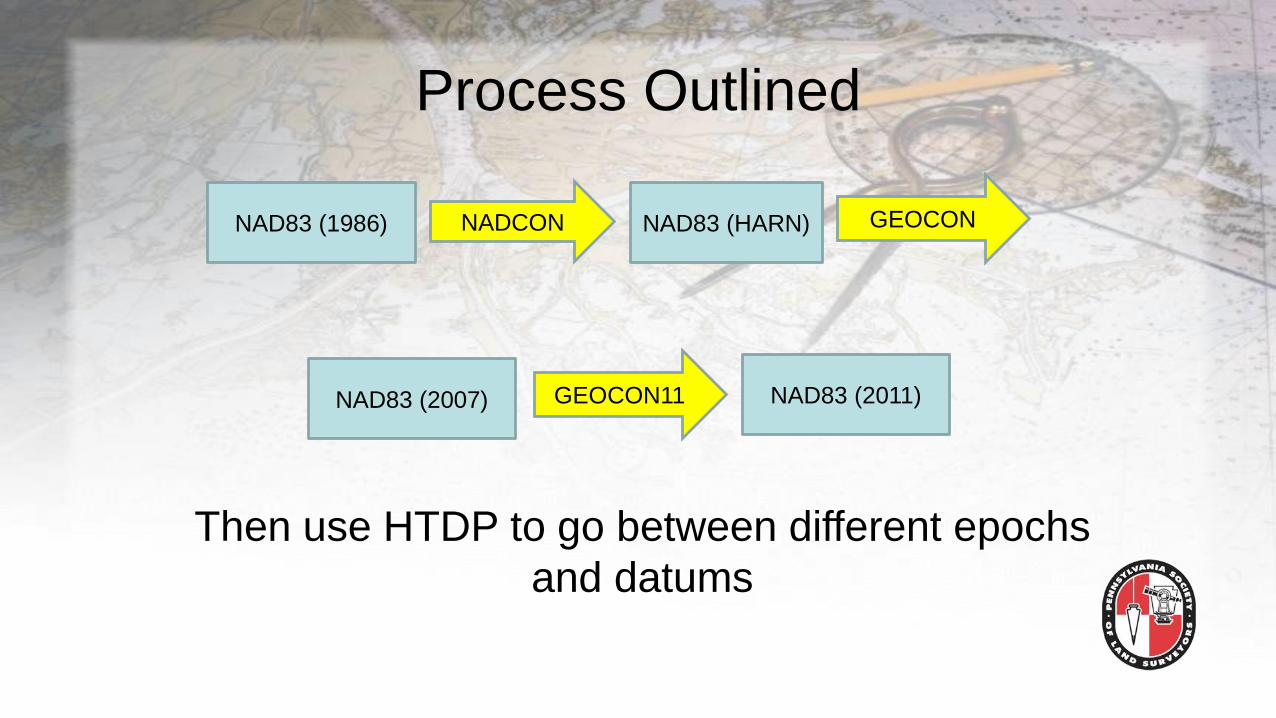
Process Outlined

NAD83 (1986) NADCON NAD83 (HARN)

GEOCON11 NAD83 (2011)NAD83 (2007)

GEOCON

Then use HTDP to go between different epochs

and datums

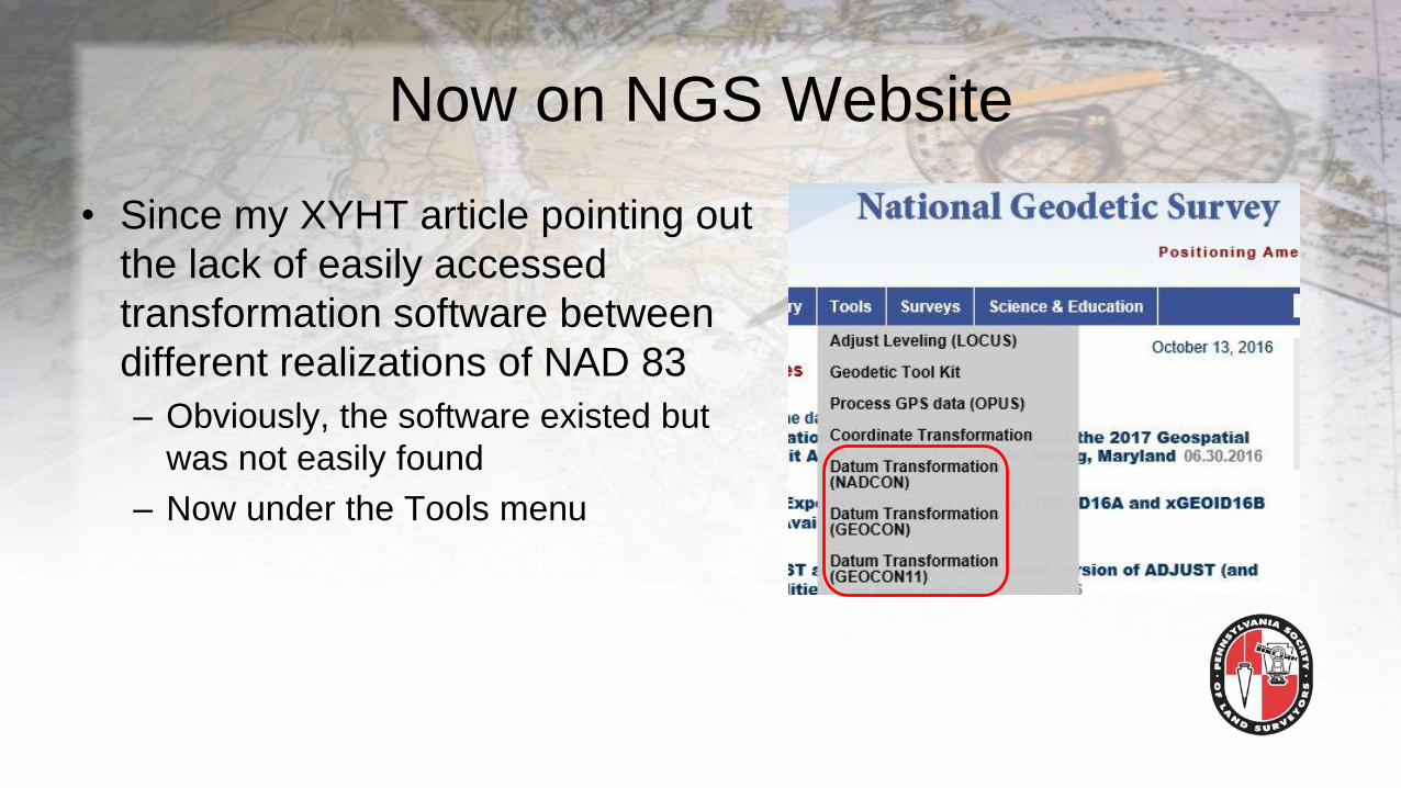
Now on NGS Website

• Since my XYHT article pointing out

the lack of easily accessed

transformation software between

different realizations of NAD 83

– Obviously, the software existed but

was not easily found

– Now under the Tools menu

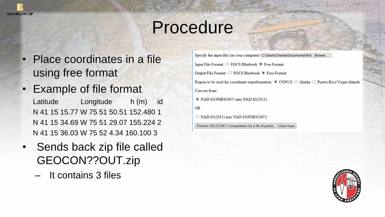
Procedure

• Place coordinates in a file

using free format

• Example of file formatLatitude Longitude h (m) id

N 41 15 15.77 W 75 51 50.51 152.480 1

N 41 15 34.69 W 75 51 29.07 155.224 2

N 41 15 36.03 W 75 52 4.34 160.100 3

• Sends back zip file called

GEOCON??OUT.zip

– It contains 3 files

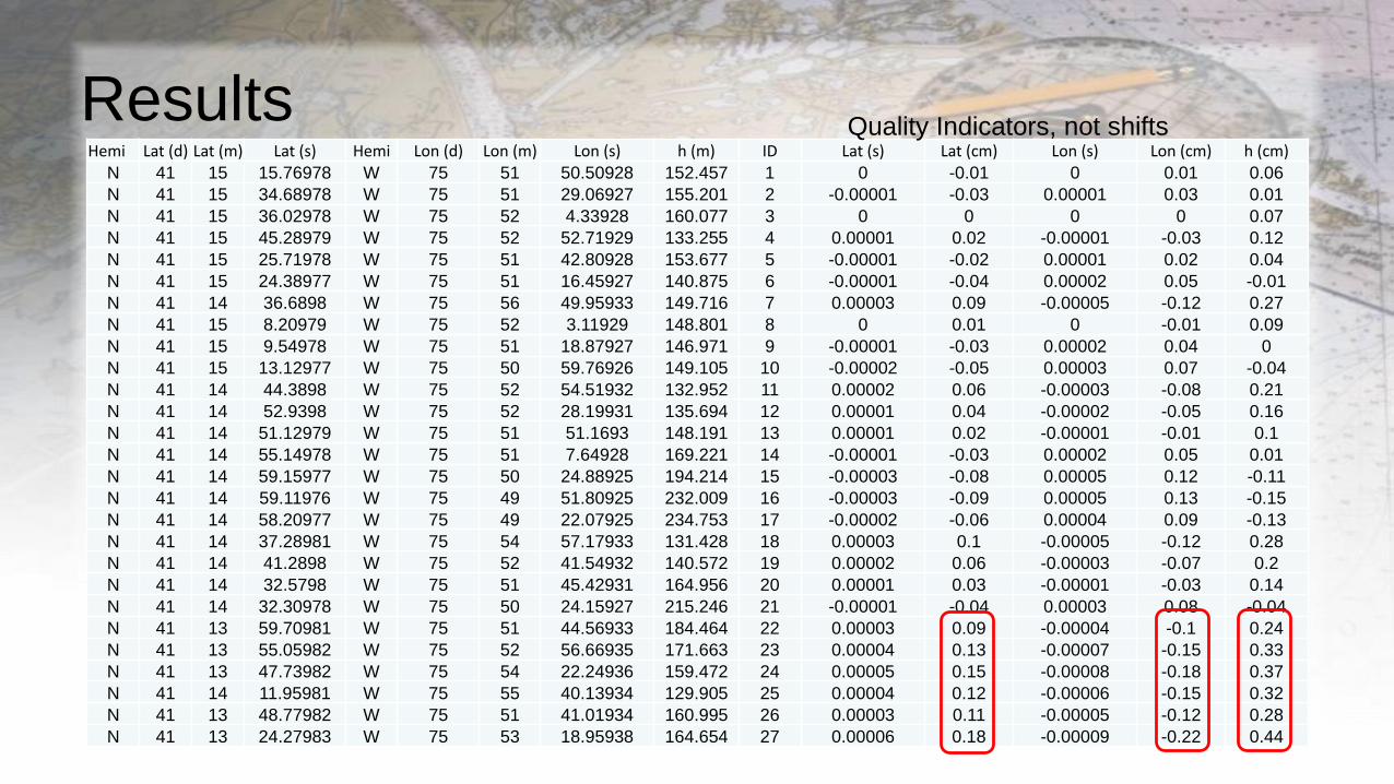
ResultsHemi Lat (d) Lat (m) Lat (s) Hemi Lon (d) Lon (m) Lon (s) h (m) ID Lat (s) Lat (cm) Lon (s) Lon (cm) h (cm)

N 41 15 15.76978 W 75 51 50.50928 152.457 1 0 -0.01 0 0.01 0.06

N 41 15 34.68978 W 75 51 29.06927 155.201 2 -0.00001 -0.03 0.00001 0.03 0.01

N 41 15 36.02978 W 75 52 4.33928 160.077 3 0 0 0 0 0.07

N 41 15 45.28979 W 75 52 52.71929 133.255 4 0.00001 0.02 -0.00001 -0.03 0.12

N 41 15 25.71978 W 75 51 42.80928 153.677 5 -0.00001 -0.02 0.00001 0.02 0.04

N 41 15 24.38977 W 75 51 16.45927 140.875 6 -0.00001 -0.04 0.00002 0.05 -0.01

N 41 14 36.6898 W 75 56 49.95933 149.716 7 0.00003 0.09 -0.00005 -0.12 0.27

N 41 15 8.20979 W 75 52 3.11929 148.801 8 0 0.01 0 -0.01 0.09

N 41 15 9.54978 W 75 51 18.87927 146.971 9 -0.00001 -0.03 0.00002 0.04 0

N 41 15 13.12977 W 75 50 59.76926 149.105 10 -0.00002 -0.05 0.00003 0.07 -0.04

N 41 14 44.3898 W 75 52 54.51932 132.952 11 0.00002 0.06 -0.00003 -0.08 0.21

N 41 14 52.9398 W 75 52 28.19931 135.694 12 0.00001 0.04 -0.00002 -0.05 0.16

N 41 14 51.12979 W 75 51 51.1693 148.191 13 0.00001 0.02 -0.00001 -0.01 0.1

N 41 14 55.14978 W 75 51 7.64928 169.221 14 -0.00001 -0.03 0.00002 0.05 0.01

N 41 14 59.15977 W 75 50 24.88925 194.214 15 -0.00003 -0.08 0.00005 0.12 -0.11

N 41 14 59.11976 W 75 49 51.80925 232.009 16 -0.00003 -0.09 0.00005 0.13 -0.15

N 41 14 58.20977 W 75 49 22.07925 234.753 17 -0.00002 -0.06 0.00004 0.09 -0.13

N 41 14 37.28981 W 75 54 57.17933 131.428 18 0.00003 0.1 -0.00005 -0.12 0.28

N 41 14 41.2898 W 75 52 41.54932 140.572 19 0.00002 0.06 -0.00003 -0.07 0.2

N 41 14 32.5798 W 75 51 45.42931 164.956 20 0.00001 0.03 -0.00001 -0.03 0.14

N 41 14 32.30978 W 75 50 24.15927 215.246 21 -0.00001 -0.04 0.00003 0.08 -0.04

N 41 13 59.70981 W 75 51 44.56933 184.464 22 0.00003 0.09 -0.00004 -0.1 0.24

N 41 13 55.05982 W 75 52 56.66935 171.663 23 0.00004 0.13 -0.00007 -0.15 0.33

N 41 13 47.73982 W 75 54 22.24936 159.472 24 0.00005 0.15 -0.00008 -0.18 0.37

N 41 14 11.95981 W 75 55 40.13934 129.905 25 0.00004 0.12 -0.00006 -0.15 0.32

N 41 13 48.77982 W 75 51 41.01934 160.995 26 0.00003 0.11 -0.00005 -0.12 0.28

N 41 13 24.27983 W 75 53 18.95938 164.654 27 0.00006 0.18 -0.00009 -0.22 0.44

Quality Indicators, not shifts

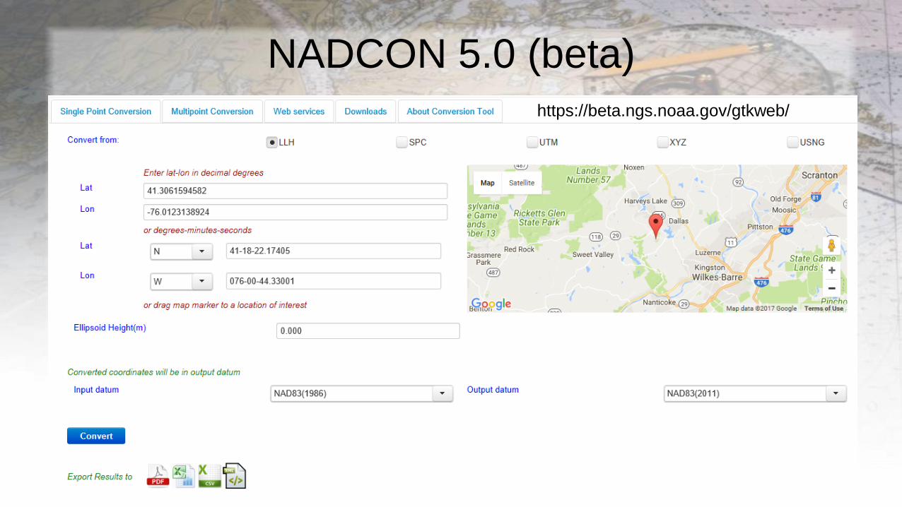
NADCON 5.0 (beta)https://beta.ngs.noaa.gov/gtkweb/

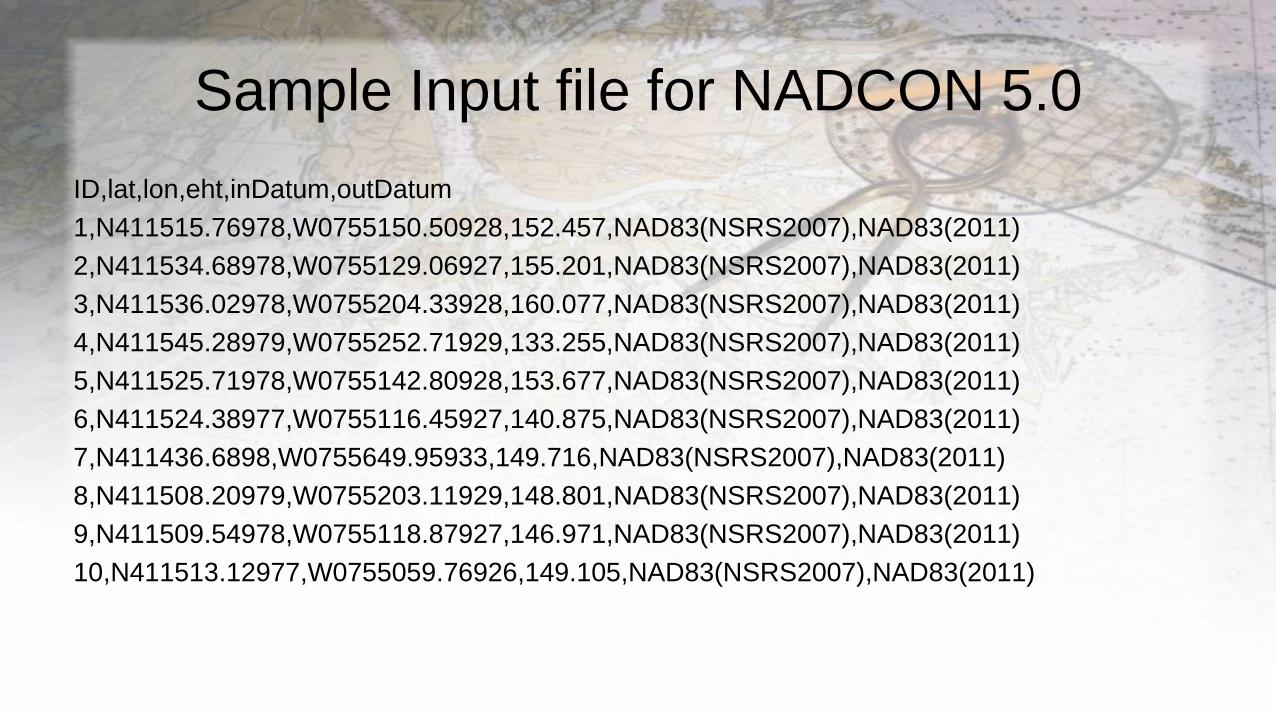
Sample Input file for NADCON 5.0

ID,lat,lon,eht,inDatum,outDatum

1,N411515.76978,W0755150.50928,152.457,NAD83(NSRS2007),NAD83(2011)

2,N411534.68978,W0755129.06927,155.201,NAD83(NSRS2007),NAD83(2011)

3,N411536.02978,W0755204.33928,160.077,NAD83(NSRS2007),NAD83(2011)

4,N411545.28979,W0755252.71929,133.255,NAD83(NSRS2007),NAD83(2011)

5,N411525.71978,W0755142.80928,153.677,NAD83(NSRS2007),NAD83(2011)

6,N411524.38977,W0755116.45927,140.875,NAD83(NSRS2007),NAD83(2011)

7,N411436.6898,W0755649.95933,149.716,NAD83(NSRS2007),NAD83(2011)

8,N411508.20979,W0755203.11929,148.801,NAD83(NSRS2007),NAD83(2011)

9,N411509.54978,W0755118.87927,146.971,NAD83(NSRS2007),NAD83(2011)

10,N411513.12977,W0755059.76926,149.105,NAD83(NSRS2007),NAD83(2011)

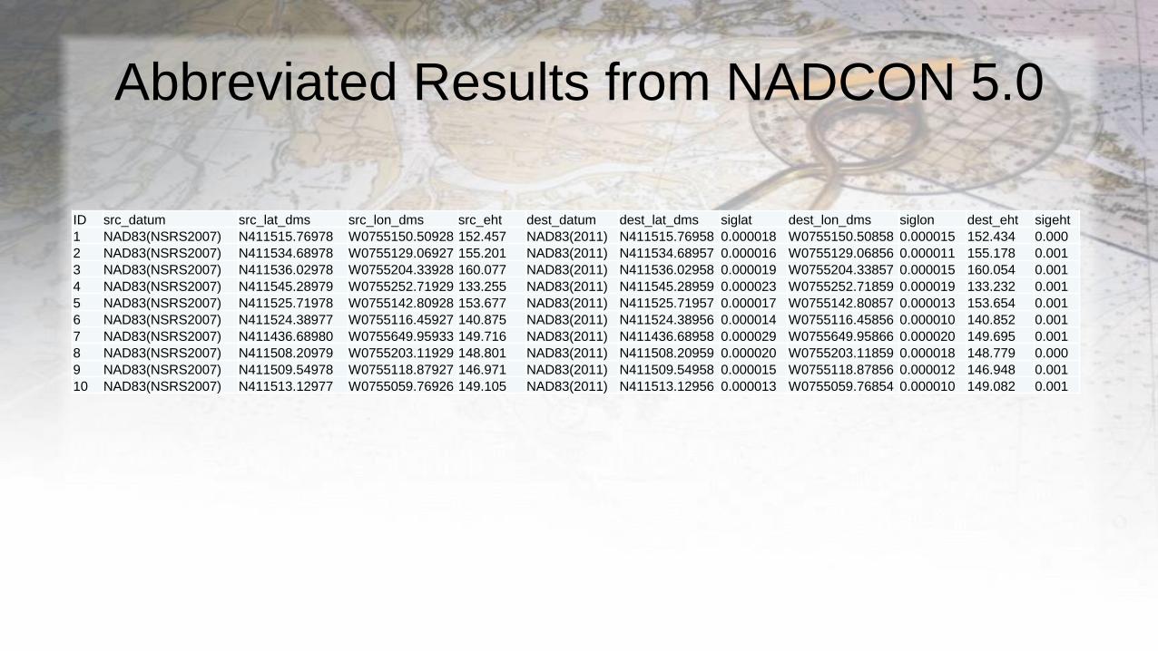
Abbreviated Results from NADCON 5.0

ID src_datum src_lat_dms src_lon_dms src_eht dest_datum dest_lat_dms siglat dest_lon_dms siglon dest_eht sigeht

1 NAD83(NSRS2007) N411515.76978 W0755150.50928 152.457 NAD83(2011) N411515.76958 0.000018 W0755150.50858 0.000015 152.434 0.000

2 NAD83(NSRS2007) N411534.68978 W0755129.06927 155.201 NAD83(2011) N411534.68957 0.000016 W0755129.06856 0.000011 155.178 0.001

3 NAD83(NSRS2007) N411536.02978 W0755204.33928 160.077 NAD83(2011) N411536.02958 0.000019 W0755204.33857 0.000015 160.054 0.001

4 NAD83(NSRS2007) N411545.28979 W0755252.71929 133.255 NAD83(2011) N411545.28959 0.000023 W0755252.71859 0.000019 133.232 0.001

5 NAD83(NSRS2007) N411525.71978 W0755142.80928 153.677 NAD83(2011) N411525.71957 0.000017 W0755142.80857 0.000013 153.654 0.001

6 NAD83(NSRS2007) N411524.38977 W0755116.45927 140.875 NAD83(2011) N411524.38956 0.000014 W0755116.45856 0.000010 140.852 0.001

7 NAD83(NSRS2007) N411436.68980 W0755649.95933 149.716 NAD83(2011) N411436.68958 0.000029 W0755649.95866 0.000020 149.695 0.001

8 NAD83(NSRS2007) N411508.20979 W0755203.11929 148.801 NAD83(2011) N411508.20959 0.000020 W0755203.11859 0.000018 148.779 0.000

9 NAD83(NSRS2007) N411509.54978 W0755118.87927 146.971 NAD83(2011) N411509.54958 0.000015 W0755118.87856 0.000012 146.948 0.001

10 NAD83(NSRS2007) N411513.12977 W0755059.76926 149.105 NAD83(2011) N411513.12956 0.000013 W0755059.76854 0.000010 149.082 0.001

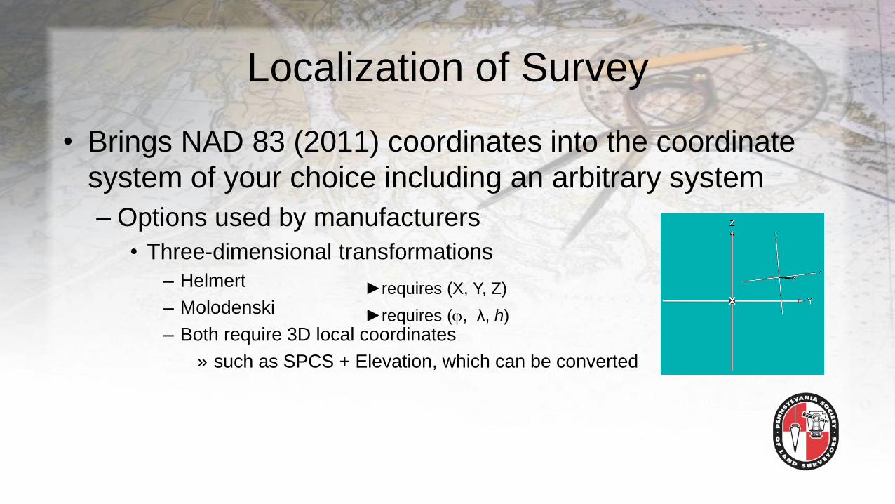
Localization of Survey

• Brings NAD 83 (2011) coordinates into the coordinate

system of your choice including an arbitrary system

– Options used by manufacturers

• Three-dimensional transformations

– Helmert

– Molodenski

– Both require 3D local coordinates

» such as SPCS + Elevation, which can be converted

►requires (X, Y, Z)

►requires (, λ, h)

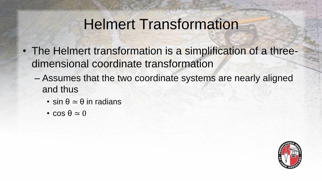
Helmert Transformation

• The Helmert transformation is a simplification of a three-

dimensional coordinate transformation

– Assumes that the two coordinate systems are nearly aligned

and thus

• sin θ ≃ θ in radians

• cos θ ≃ 0

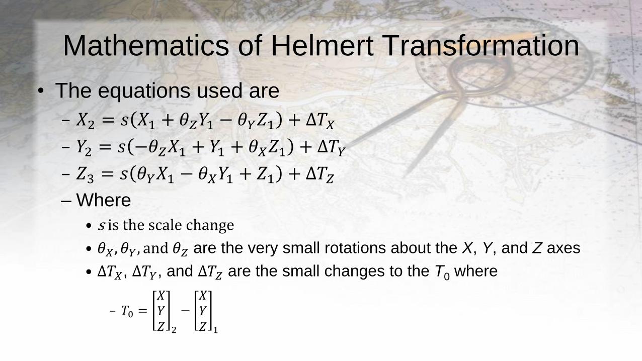
Mathematics of Helmert Transformation

• The equations used are

– 𝑋2 = 𝑠 𝑋1 + 𝜃𝑍𝑌1 − 𝜃𝑌𝑍1 + ∆𝑇𝑋

– 𝑌2 = 𝑠 −𝜃𝑍𝑋1 + 𝑌1 + 𝜃𝑋𝑍1 + ∆𝑇𝑌

– 𝑍3 = 𝑠 𝜃𝑌𝑋1 − 𝜃𝑋𝑌1 + 𝑍1 + ∆𝑇𝑍

– Where

• s is the scale change

• 𝜃𝑋, 𝜃𝑌, and 𝜃𝑍 are the very small rotations about the X, Y, and Z axes

• ∆𝑇𝑋, ∆𝑇𝑌, and ∆𝑇𝑍 are the small changes to the T0 where

– 𝑇0 =𝑋𝑌𝑍 2

−𝑋𝑌𝑍 1

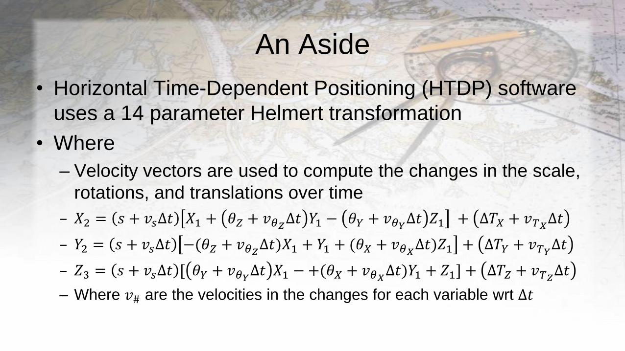
An Aside

• Horizontal Time-Dependent Positioning (HTDP) software

uses a 14 parameter Helmert transformation

• Where

– Velocity vectors are used to compute the changes in the scale,

rotations, and translations over time

– 𝑋2 = 𝑠 + 𝑣𝑠∆𝑡 𝑋1 + 𝜃𝑍 + 𝑣𝜃𝑍∆𝑡 𝑌1 − 𝜃𝑌 + 𝑣𝜃𝑌

∆𝑡 𝑍1 + ∆𝑇𝑋 + 𝑣𝑇𝑋∆𝑡

– 𝑌2 = 𝑠 + 𝑣𝑠∆𝑡 −(𝜃𝑍 + 𝑣𝜃𝑍∆𝑡)𝑋1 + 𝑌1 + (𝜃𝑋 + 𝑣𝜃𝑋

∆𝑡)𝑍1 + ∆𝑇𝑌 + 𝑣𝑇𝑌∆𝑡

– 𝑍3 = 𝑠 + 𝑣𝑠∆𝑡 [ 𝜃𝑌 + 𝑣𝜃𝑌∆𝑡 𝑋1 − +(𝜃𝑋 + 𝑣𝜃𝑋

∆𝑡)𝑌1 + 𝑍1] + ∆𝑇𝑍 + 𝑣𝑇𝑍∆𝑡

– Where 𝑣# are the velocities in the changes for each variable wrt ∆𝑡

Localization of Survey

• Brings NAD 83 (2011) coordinates into the coordinate

system of your choice including an arbitrary system

– Option typically used by manufacturers

• Two + One method

– Most common since it can use any coordinate system

» Including arbitrary systems like (5000, 5000, 100)!

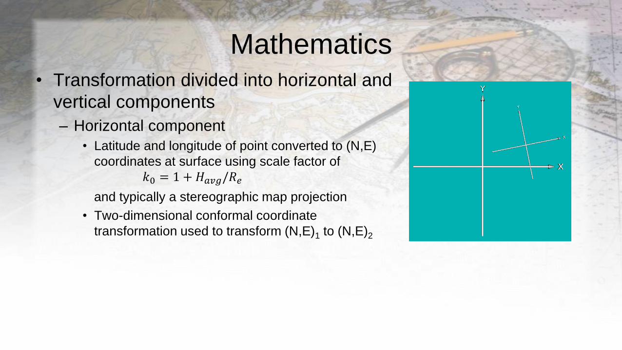
Mathematics• Transformation divided into horizontal and

vertical components

– Horizontal component

• Latitude and longitude of point converted to (N,E)

coordinates at surface using scale factor of

𝑘0 = 1 + 𝐻𝑎𝑣𝑔/𝑅𝑒

and typically a stereographic map projection

• Two-dimensional conformal coordinate

transformation used to transform (N,E)1 to (N,E)2

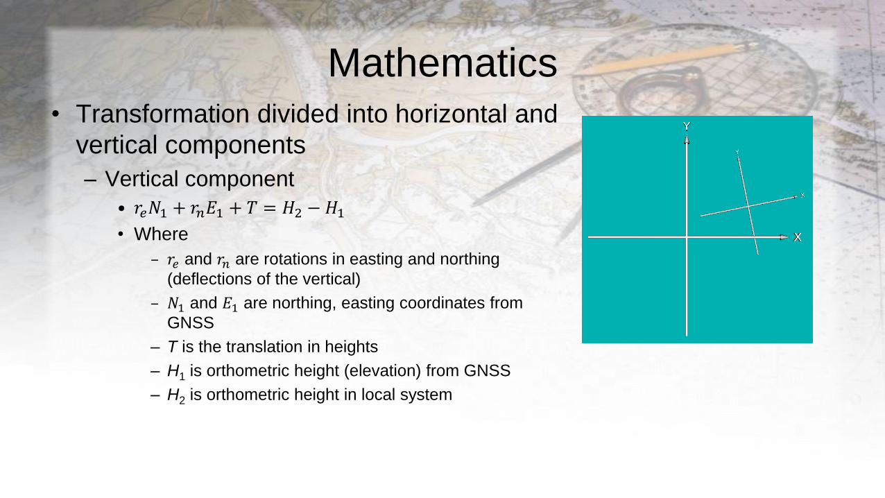
Mathematics• Transformation divided into horizontal and

vertical components

– Vertical component

• 𝑟𝑒𝑁1 + 𝑟𝑛𝐸1 + 𝑇 = 𝐻2 − 𝐻1

• Where

– 𝑟𝑒 and 𝑟𝑛 are rotations in easting and northing

(deflections of the vertical)

– 𝑁1 and 𝐸1 are northing, easting coordinates from

GNSS

– T is the translation in heights

– H1 is orthometric height (elevation) from GNSS

– H2 is orthometric height in local system

Best Practices

• Control must be in proper locations

• A minimum of

– 4 horizontal control points

– 4 vertical control points

– 1 point in each quadrant of the project near edges of project, preferred

– Include any crucial design points such as control on bridges

– Check Points: Have additional control points that are NOT included in the

localization to use as checks after the localization

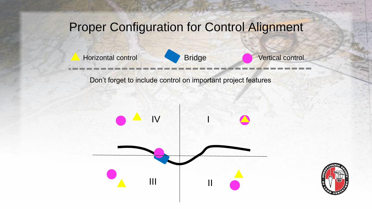
Proper Configuration for Control Alignment

Horizontal control Vertical control

IIV

III II

Bridge

Don’t forget to include control on important project features

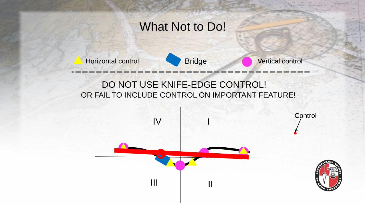
What Not to Do!

Horizontal control Vertical control

IIV

III II

Bridge

DO NOT USE KNIFE-EDGE CONTROL!OR FAIL TO INCLUDE CONTROL ON IMPORTANT FEATURE!

Control

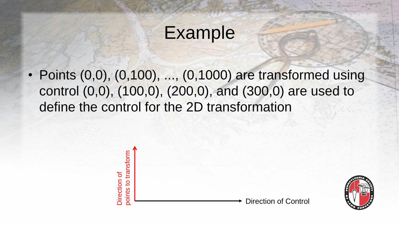
Example

• Points (0,0), (0,100), ..., (0,1000) are transformed using

control (0,0), (100,0), (200,0), and (300,0) are used to

define the control for the 2D transformation

Direction of ControlDir

ection o

f

poin

ts to t

ransfo

rm

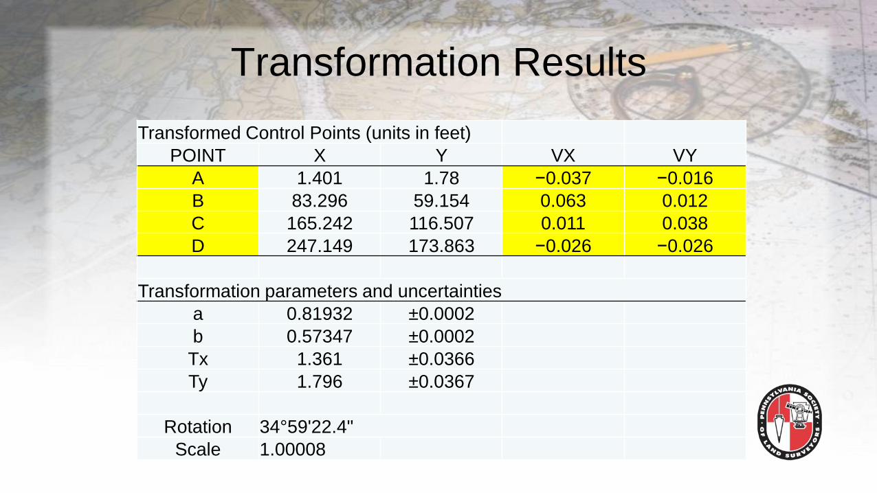
Transformation Results

Transformed Control Points (units in feet)

POINT X Y VX VY

A 1.401 1.78 −0.037 −0.016

B 83.296 59.154 0.063 0.012

C 165.242 116.507 0.011 0.038

D 247.149 173.863 −0.026 −0.026

Transformation parameters and uncertainties

a 0.81932 ±0.0002

b 0.57347 ±0.0002

Tx 1.361 ±0.0366

Ty 1.796 ±0.0367

Rotation 34°59'22.4"

Scale 1.00008

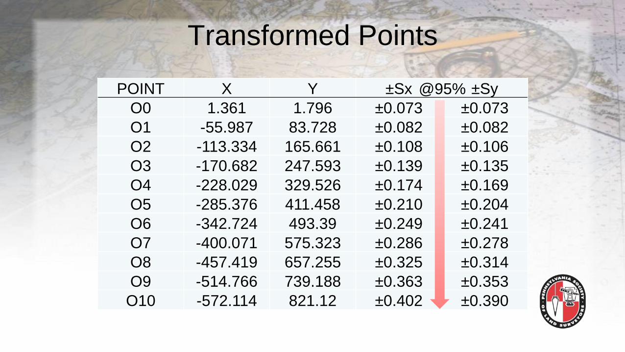
Transformed Points

POINT X Y ±Sx ±Sy

O0 1.361 1.796 ±0.073 ±0.073

O1 -55.987 83.728 ±0.082 ±0.082

O2 -113.334 165.661 ±0.108 ±0.106

O3 -170.682 247.593 ±0.139 ±0.135

O4 -228.029 329.526 ±0.174 ±0.169

O5 -285.376 411.458 ±0.210 ±0.204

O6 -342.724 493.39 ±0.249 ±0.241

O7 -400.071 575.323 ±0.286 ±0.278

O8 -457.419 657.255 ±0.325 ±0.314

O9 -514.766 739.188 ±0.363 ±0.353

O10 -572.114 821.12 ±0.402 ±0.390

@95%

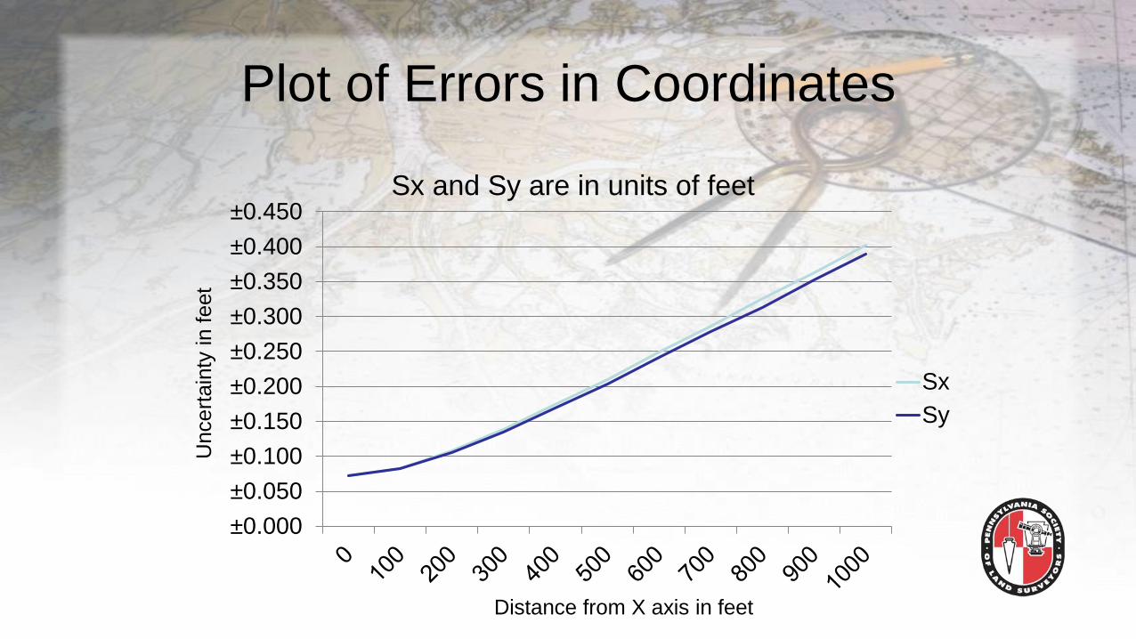
Plot of Errors in Coordinates

Sx and Sy are in units of feet

Distance from X axis in feet

Uncert

ain

ty in f

eet

±0.000

±0.050

±0.100

±0.150

±0.200

±0.250

±0.300

±0.350

±0.400

±0.450

Sx

Sy

Remember

• Extrapolation of data is bad!

• Interpolation of data is GOOD!

– So always try to have control near edges of project

• Always include a geoid model when performing a

localization

– Geoid model is a systematic error, which should not be part of

the adjustment

Remember

• Perform localization only once per project

– Failure to do so will result in creating different realizations for

the same points (i.e. varied coordinates)

• Caused by errors in GNSS observations

– Do it once and do it correctly!

• Share localization with other field crews on same project

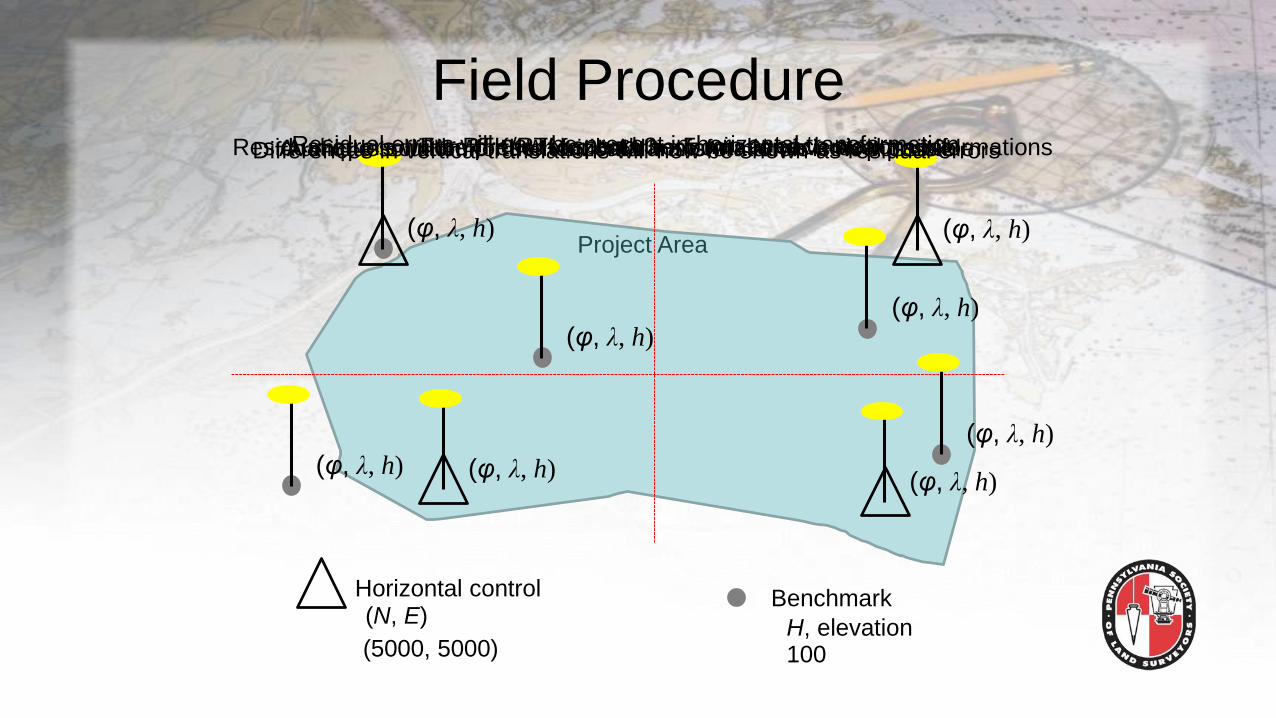
Field Procedure

BenchmarkHorizontal control

(φ, λ, h)

(φ, λ, h)

(φ, λ, h)

(φ, λ, h)

(φ, λ, h)

(φ, λ, h)

(φ, λ, h)

(φ, λ, h)

(N, E)

(5000, 5000)H, elevation100

Project Area

For RTK/RTN spend 3 – 5 min at each stationDifferences in vertical translations will now be shown as residual errorsA unique solution for the horizontal transformation is now possibleA unique solution for the vertical transformation is now possibleResidual errors will now be present in horizontal transformationResidual errors will be present for both horizontal and vertical transformations

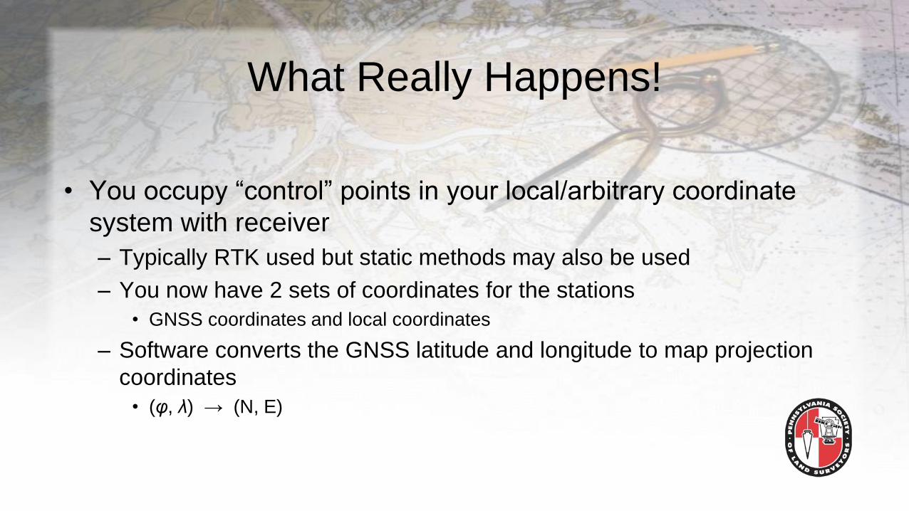
What Really Happens!

• You occupy “control” points in your local/arbitrary coordinate

system with receiver

– Typically RTK used but static methods may also be used

– You now have 2 sets of coordinates for the stations

• GNSS coordinates and local coordinates

– Software converts the GNSS latitude and longitude to map projection

coordinates

• (φ, λ) → (N, E)

Conversion of GNSS Coordinates

• Any map projection can be used

• The choice of many manufacturers is an oblique

stereographic map projection due to its simplicity

– Only requires:

• 𝑘0 = 1 +ℎ0

𝑅𝐺; where h0 is a geodetic height and RG = Gaussian mean

radius at the grid origin

• Grid origin 𝜑0, λ0

• 𝑅𝐺 =𝑎 1−𝑒2

1−𝑒2 sin2 𝜑

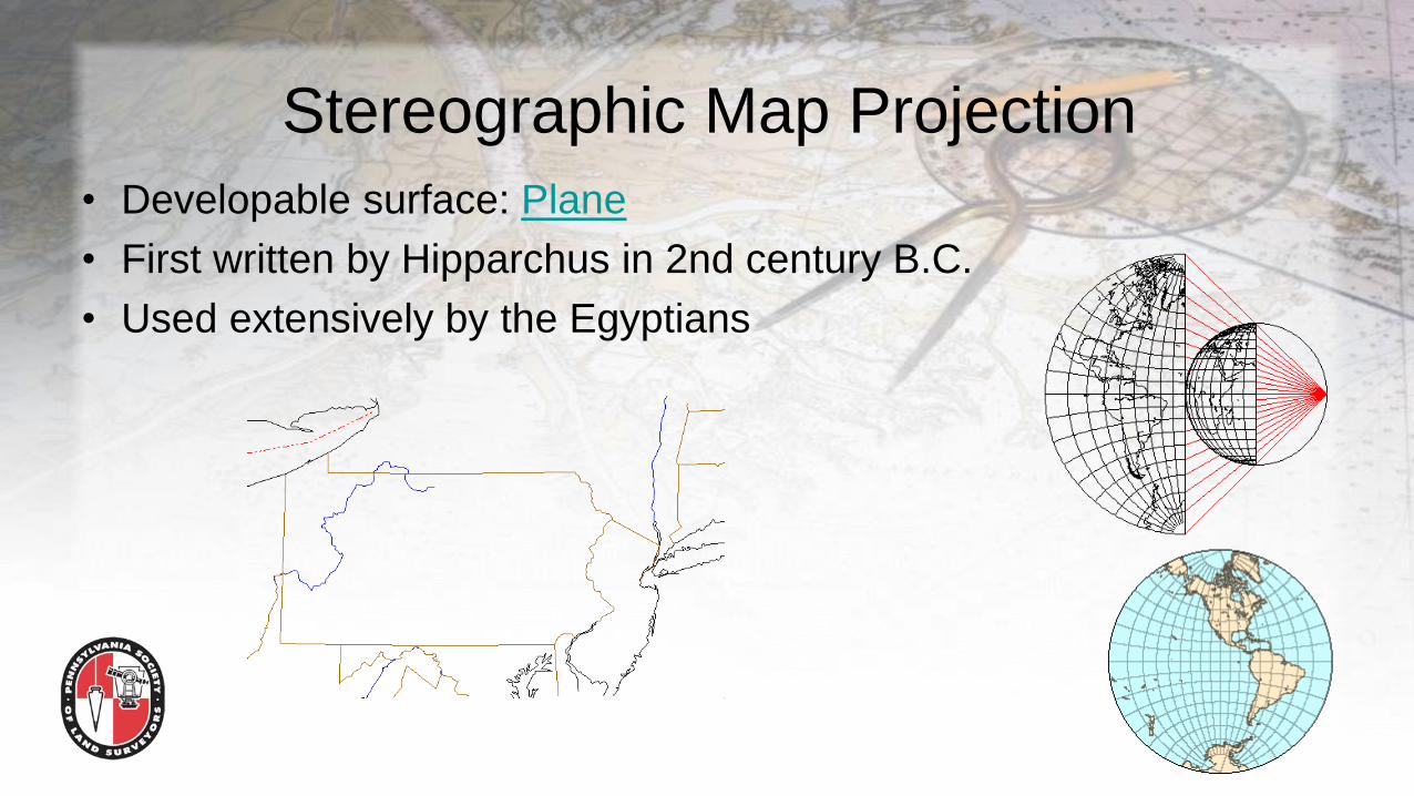
Stereographic Map Projection

• Developable surface: Plane

• First written by Hipparchus in 2nd century B.C.

• Used extensively by the Egyptians

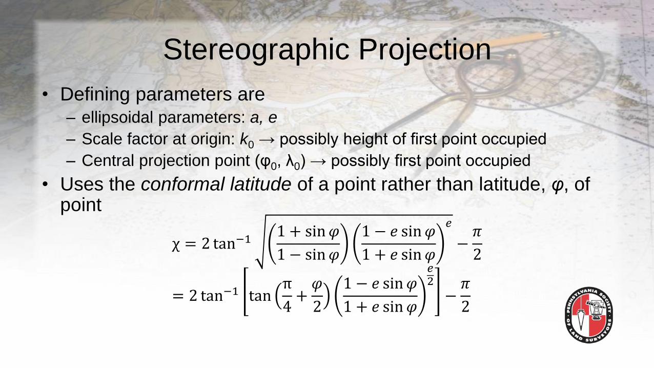
Stereographic Projection

• Defining parameters are– ellipsoidal parameters: a, e

– Scale factor at origin: k0 → possibly height of first point occupied

– Central projection point (φ0, λ0) → possibly first point occupied

• Uses the conformal latitude of a point rather than latitude, φ, of point

χ = 2 tan−11 + sin 𝜑

1 − sin 𝜑

1 − 𝑒 sin 𝜑

1 + 𝑒 sin 𝜑

𝑒

−𝜋

2

= 2 tan−1 tanπ

4+

𝜑

2

1 − 𝑒 sin 𝜑

1 + 𝑒 sin 𝜑

𝑒2

−𝜋

2

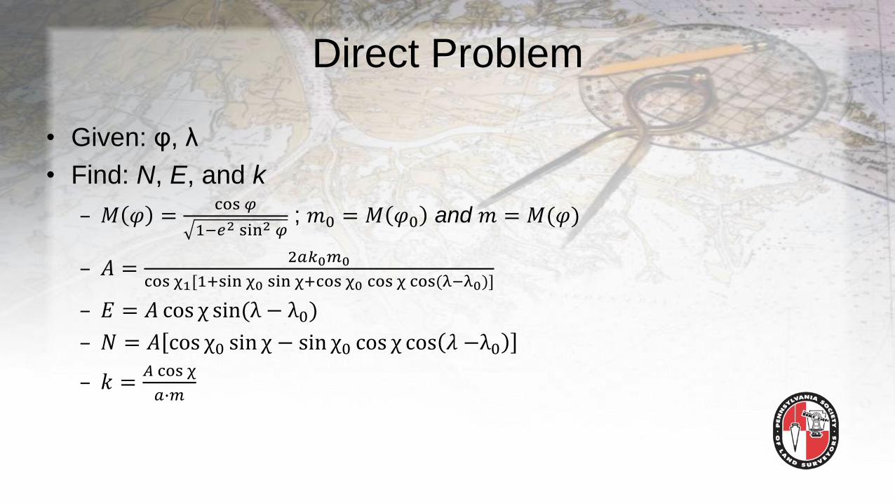
Direct Problem

• Given: φ, λ

• Find: N, E, and k

– 𝑀 𝜑 =cos 𝜑

1−𝑒2 sin2 𝜑; 𝑚0 = 𝑀 𝜑0 and 𝑚 = 𝑀(𝜑)

– 𝐴 =2𝑎𝑘0𝑚0

cos χ1[1+sin χ0 sin χ+cos χ0 cos χ cos(λ−λ0)]

– 𝐸 = 𝐴 cos χ sin(λ − λ0)

– 𝑁 = 𝐴 cos χ0 sin χ − sin χ0 cos χ cos 𝜆 −λ0

– 𝑘 =𝐴 cos χ

𝑎∙𝑚

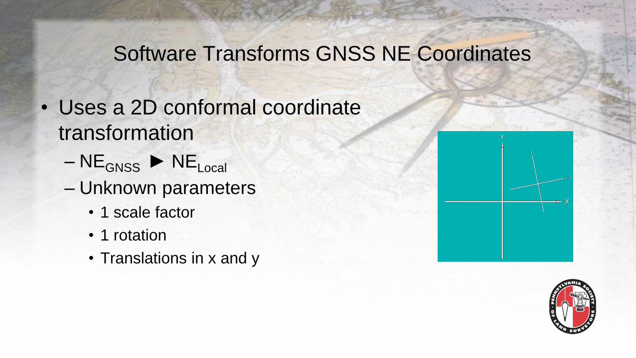
Software Transforms GNSS NE Coordinates

• Uses a 2D conformal coordinate

transformation

– NEGNSS

– Unknown parameters

• 1 scale factor

• 1 rotation

• Translations in x and y

► NELocal

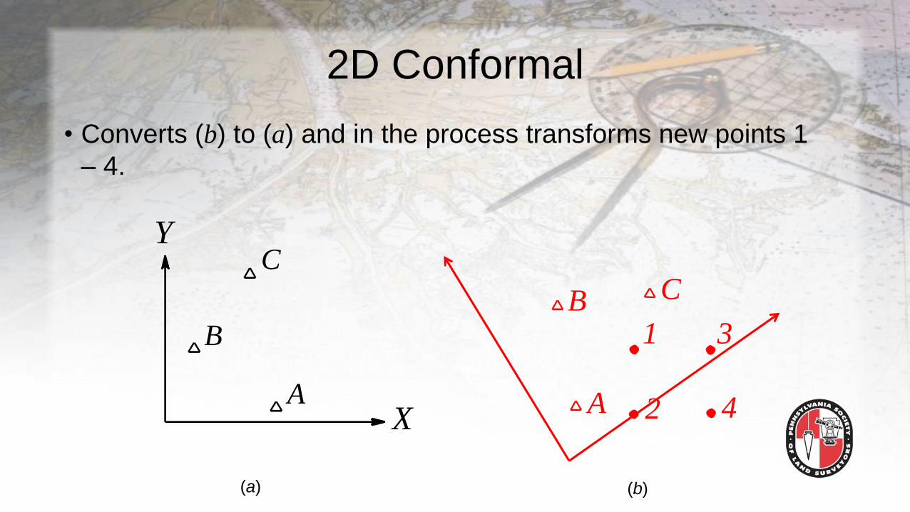
2D Conformal

Y

X

B

C

A

• Converts (b) to (a) and in the process transforms new points 1

– 4.

1 3

42A

B C

(a) (b)

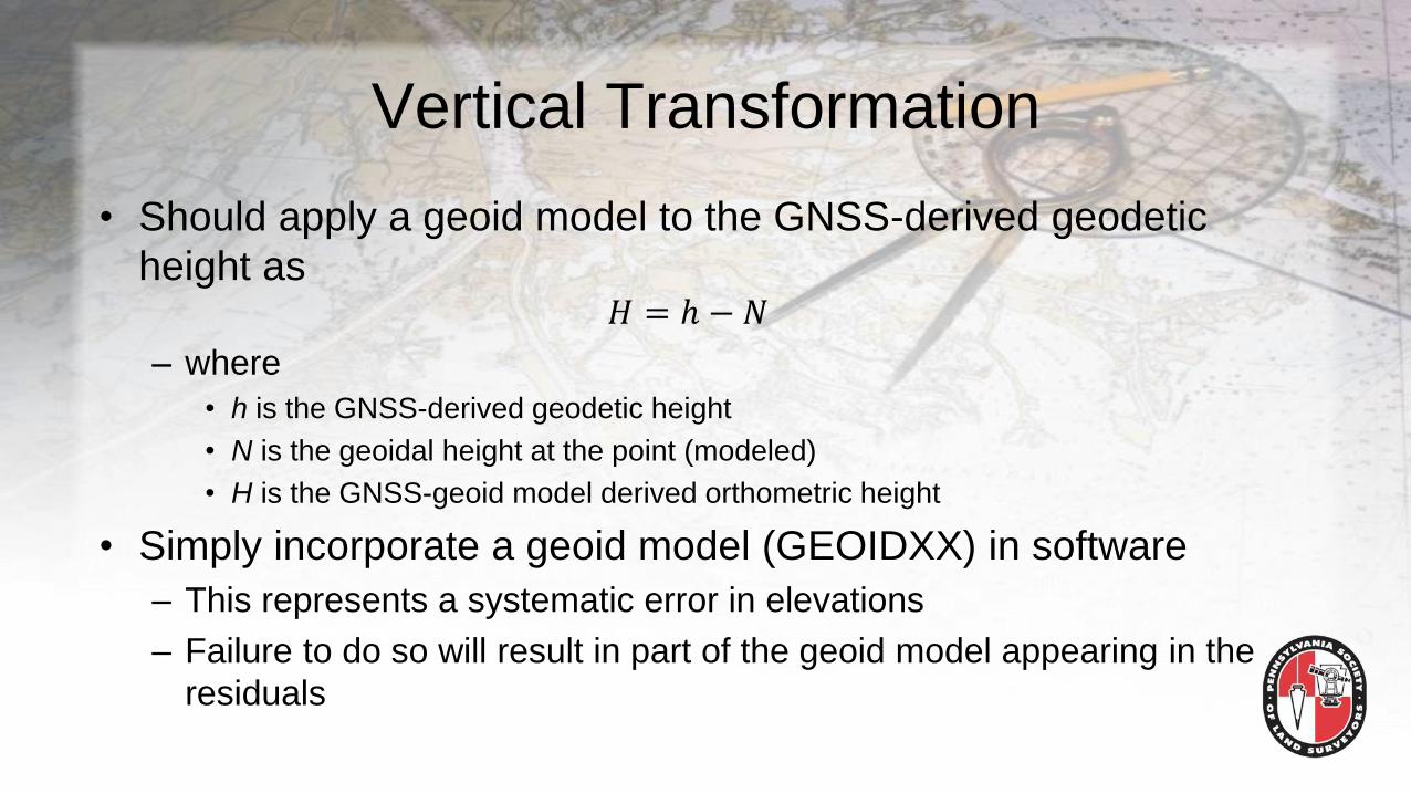
Vertical Transformation

• Should apply a geoid model to the GNSS-derived geodetic

height as 𝐻 = ℎ − 𝑁

– where

• h is the GNSS-derived geodetic height

• N is the geoidal height at the point (modeled)

• H is the GNSS-geoid model derived orthometric height

• Simply incorporate a geoid model (GEOIDXX) in software

– This represents a systematic error in elevations

– Failure to do so will result in part of the geoid model appearing in the

residuals

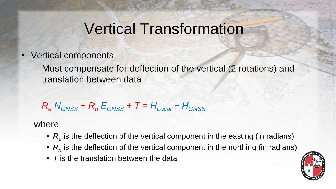
Vertical Transformation

• Vertical components

– Must compensate for deflection of the vertical (2 rotations) and

translation between data

Re NGNSS + Rn EGNSS + T = HLocal − HGNSS

where

• Re is the deflection of the vertical component in the easting (in radians)

• Rn is the deflection of the vertical component in the northing (in radians)

• T is the translation between the data

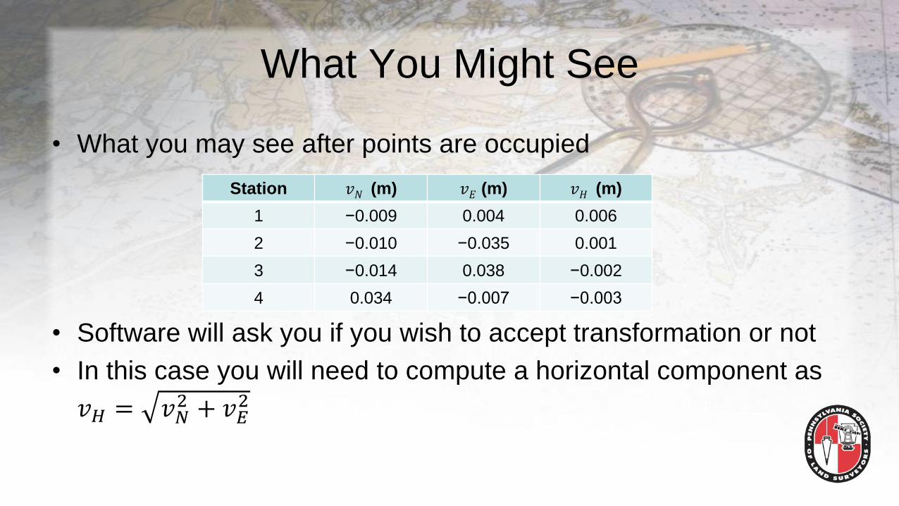
What You Might See

• What you may see after points are occupied

• Software will ask you if you wish to accept transformation or not

• In this case you will need to compute a horizontal component as

𝑣𝐻 = 𝑣𝑁2 + 𝑣𝐸

2

Station 𝑣𝑁 (m) 𝑣𝐸 (m) 𝑣𝐻 (m)

1 −0.009 0.004 0.006

2 −0.010 −0.035 0.001

3 −0.014 0.038 −0.002

4 0.034 −0.007 −0.003

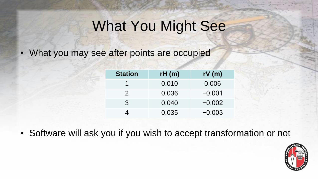
What You Might See

• What you may see after points are occupied

• Software will ask you if you wish to accept transformation or not

Station rH (m) rV (m)

1 0.010 0.006

2 0.036 −0.001

3 0.040 −0.002

4 0.035 −0.003

Are the Residuals Acceptable?

• What are acceptable residuals?

– That depends!!!

• How good are the local control?

• How good are the GNSS-derived coordinates?

– Did you occupy the common points for 10 epochs or 180 – 300 epochs?

• How good are the instrument setups?

– Handheld receiver

– Bipod/Tripod support of rod

– Specifications for circular level vial and its adjustment

• When was the last time you checked your rod bubble?

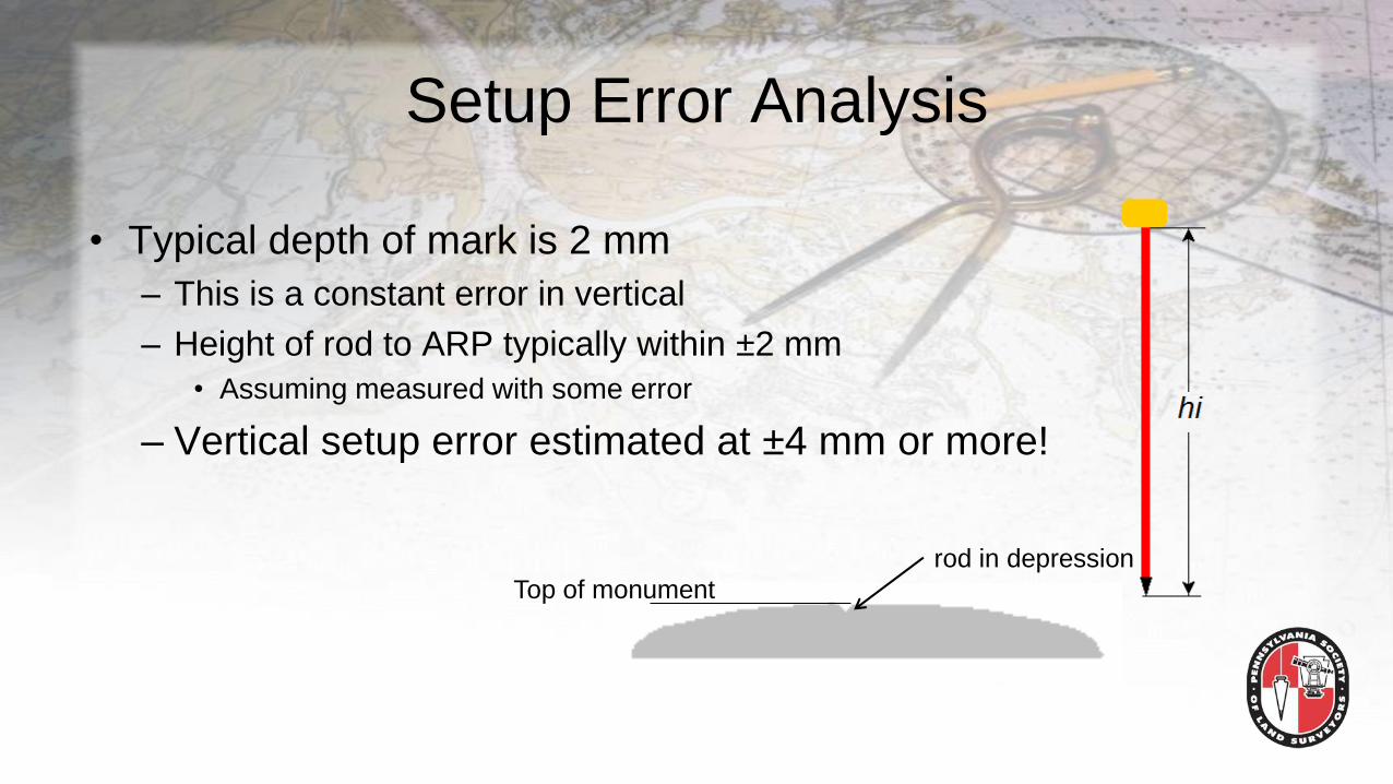
Setup Error Analysis

• Typical depth of mark is 2 mm

– This is a constant error in vertical

– Height of rod to ARP typically within ±2 mm

• Assuming measured with some error

– Vertical setup error estimated at ±4 mm or more!

rod in depression

Top of monument

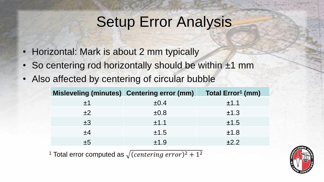
Setup Error Analysis

• Horizontal: Mark is about 2 mm typically

• So centering rod horizontally should be within ±1 mm

• Also affected by centering of circular bubble

Misleveling (minutes) Centering error (mm) Total Error1 (mm)

±1 ±0.4 ±1.1

±2 ±0.8 ±1.3

±3 ±1.1 ±1.5

±4 ±1.5 ±1.8

±5 ±1.9 ±2.2

1 Total error computed as 𝑐𝑒𝑛𝑡𝑒𝑟𝑖𝑛𝑔 𝑒𝑟𝑟𝑜𝑟 2 + 12

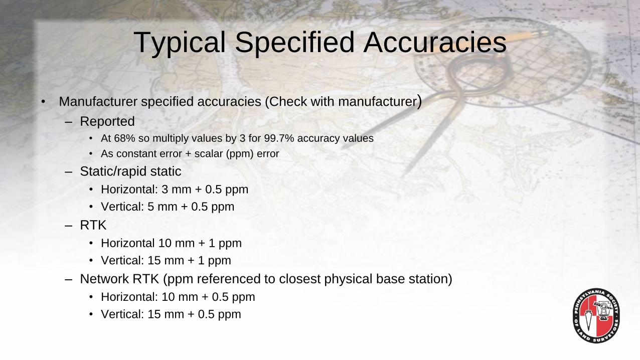
Typical Specified Accuracies

• Manufacturer specified accuracies (Check with manufacturer)

– Reported

• At 68% so multiply values by 3 for 99.7% accuracy values

• As constant error + scalar (ppm) error

– Static/rapid static

• Horizontal: 3 mm + 0.5 ppm

• Vertical: 5 mm + 0.5 ppm

– RTK

• Horizontal 10 mm + 1 ppm

• Vertical: 15 mm + 1 ppm

– Network RTK (ppm referenced to closest physical base station)

• Horizontal: 10 mm + 0.5 ppm

• Vertical: 15 mm + 0.5 ppm

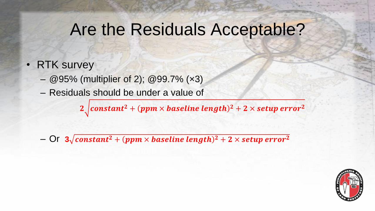
Are the Residuals Acceptable?

• RTK survey

– @95% (multiplier of 2); @99.7% (×3)

– Residuals should be under a value of

𝟐 𝒄𝒐𝒏𝒔𝒕𝒂𝒏𝒕𝟐 + 𝒑𝒑𝒎 × 𝒃𝒂𝒔𝒆𝒍𝒊𝒏𝒆 𝒍𝒆𝒏𝒈𝒕𝒉 𝟐 + 𝟐 × 𝒔𝒆𝒕𝒖𝒑 𝒆𝒓𝒓𝒐𝒓𝟐

– Or 3 𝒄𝒐𝒏𝒔𝒕𝒂𝒏𝒕𝟐 + 𝒑𝒑𝒎 × 𝒃𝒂𝒔𝒆𝒍𝒊𝒏𝒆 𝒍𝒆𝒏𝒈𝒕𝒉 𝟐 + 𝟐 × 𝒔𝒆𝒕𝒖𝒑 𝒆𝒓𝒓𝒐𝒓𝟐

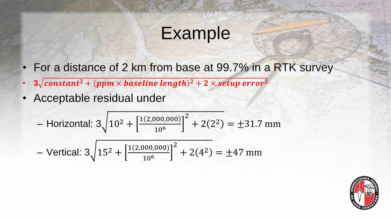
Example

• For a distance of 2 km from base at 99.7% in a RTK survey

• 3 𝒄𝒐𝒏𝒔𝒕𝒂𝒏𝒕𝟐 + 𝒑𝒑𝒎 × 𝒃𝒂𝒔𝒆𝒍𝒊𝒏𝒆 𝒍𝒆𝒏𝒈𝒕𝒉 𝟐 + 𝟐 × 𝒔𝒆𝒕𝒖𝒑 𝒆𝒓𝒓𝒐𝒓𝟐

• Acceptable residual under

– Horizontal: 3 102 +1 2,000,000

106

2+ 2 22 = ±31.7 mm

– Vertical: 3 152 +1(2,000,000)

106

2+ 2 42 = ±47 mm

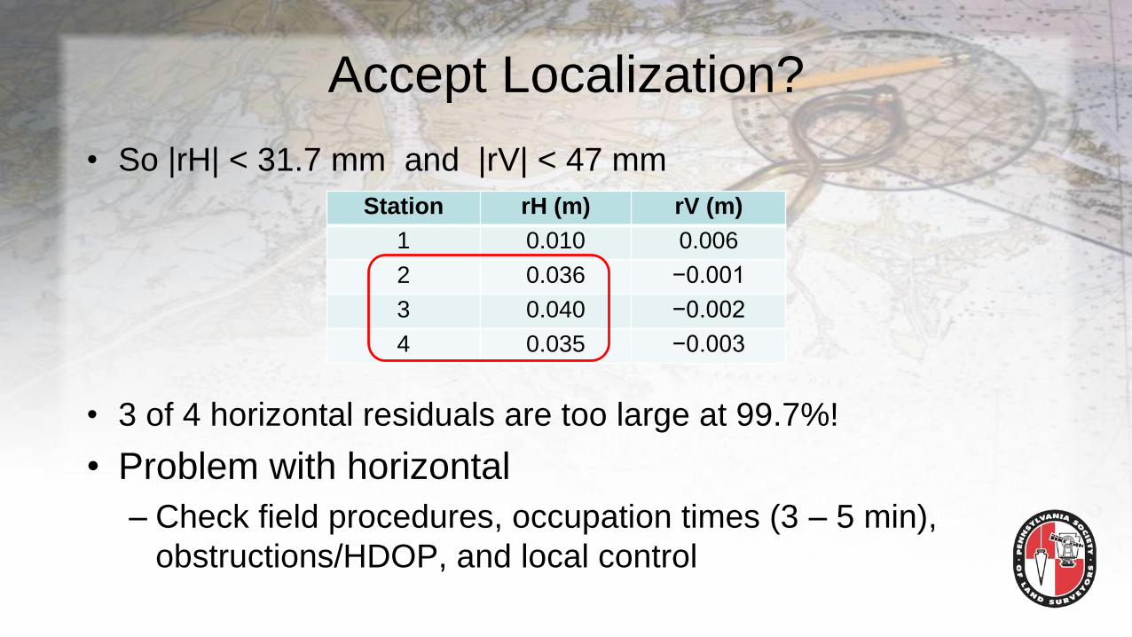
Accept Localization?

• So |rH| < 31.7 mm and |rV| < 47 mm

• 3 of 4 horizontal residuals are too large at 99.7%!

• Problem with horizontal

– Check field procedures, occupation times (3 – 5 min),

obstructions/HDOP, and local control

Station rH (m) rV (m)

1 0.010 0.006

2 0.036 −0.001

3 0.040 −0.002

4 0.035 −0.003

Food for Thought

Localization and a Boundary Survey

• You can use this when most of the corners are visible but do not

agree with record

1. Compute arbitrary horizontal coordinates for corners from record

document

2. Localize a GNSS survey to the arbitrary record coordinates

3. View the horizontal residuals of the localized survey to see

where the largest disagreement from the record exists

– Ignore any vertical components

Summary

• You need the control to surround the project area

• Horizontal control (4 or more recommended) to properly

define scale and rotation

– At least one in each quadrant of project

– Include important design points!

Summary

• You need the control to surround the project area

– Vertical control (4 or more recommended) to properly orient

level surface.

• At lease one in each quadrant of the project

• Should be at/near edges of project

• Include a GEOID model to remove systematic errors

• Include “important” design points!

Summary

• Have additional control to use as a check after the

localization

• Never perform a localization more than once for a project

– Doing it more than once will

• Create different realizations of the transformation

• You will be creating multiple coordinate systems

• Analyze residuals, remove bad observations, then accept

localization

Questions?