Performance Analysis of Demand Response …kunz-pc.sce.carleton.ca/Thesis/BichengThesis.pdfPerformance Analysis of Demand Response System on top of UMTS Network Submitted by Bicheng

PerformancePerformancePerformancePerformanceAnalysisAnalysisAnalysisAnalysis ofofofof DemandDemandDemandDemand ResponseResponseResponseResponse SystemSystemSystemSystem onononon toptoptoptop ofofofof

UMTSUMTSUMTSUMTS NetworkNetworkNetworkNetwork

By

BichengBichengBichengBicheng HuangHuangHuangHuang

A thesis submitted to

The Faculty of Graduate Studies and Research

in partial fulfilment of

the degree requirements of

MasterMasterMasterMaster ofofofof ScienceScienceScienceScience (M.Sc.)(M.Sc.)(M.Sc.)(M.Sc.) inininin InformationInformationInformationInformation andandandand SystemsSystemsSystemsSystems ScienceScienceScienceScience (ISS)(ISS)(ISS)(ISS)

Department of Systems and Computer Engineering

Carleton University

Ottawa, Ontario, Canada

Nov. 2008

Copyright ©

2008 – Bicheng Huang

ii

The undersigned recommend to

the Faculty of Graduate Studies and Research

acceptance of the thesis

PerformancePerformancePerformancePerformanceAnalysisAnalysisAnalysisAnalysis ofofofof DemandDemandDemandDemand ResponseResponseResponseResponse SystemSystemSystemSystem onononon toptoptoptop ofofofof UMTSUMTSUMTSUMTS

NetworkNetworkNetworkNetwork

Submitted by BichengBichengBichengBicheng HuangHuangHuangHuang

in partial fulfilment of the requirements for the degree of

MasterMasterMasterMaster ofofofof ScienceScienceScienceScience (M.Sc.)(M.Sc.)(M.Sc.)(M.Sc.) inininin InformationInformationInformationInformation andandandand SystemsSystemsSystemsSystems ScienceScienceScienceScience (ISS)(ISS)(ISS)(ISS)

__________________________________________________

Thomas Kunz, Thesis Supervisor

__________________________________________________

Victor Aitken, Chair, Department of Systems and Computer Engineering

Carleton University

2008

iii

AbstractAbstractAbstractAbstract

Demand Response mechanisms help power grid operators to dynamically manage

demand from customers and maintain a stable power supply level. With the

development of 3G technologies, many services can co-exist simultaneously. A

common 3G technology is UMTS, currently being deployed in a number of countries.

It is used as the platform for our task.

We explore the impact of DR Service on other services within the UMTS framework:

Compared to TCP, UDP as a transport protocol is a better choice for DR Service;

Different physical environments for DR application are evaluated; The impact that DR

Service has on RRC Service can be limited to minimum if the frequency of DR

Service is controlled.

XML-based DR application introduces redundant data, larger DR messages have a

more significant impact on RRC Service. XML compression technologies can reduce

the size of DR messages to 20%-50% of the original documents.

iv

DedicationsDedicationsDedicationsDedications

This is for my parents and my grandmother, who have been there for me from my

childhood, to my university years. Their continuing support and encouragement have

enabled me to accomplish both professional and personal goals. I thank them for their

unconditional love.

v

AcknowledgementsAcknowledgementsAcknowledgementsAcknowledgements

I would like to thank my supervisor Thomas Kunz for his guidance and support in the

last two years. His directions and instructions have challenged me to reach my

scholastic achievements.

vi

TableTableTableTable ofofofof ContentsContentsContentsContents

AbstractAbstractAbstractAbstract iiiiiiiiiiii

DedicationsDedicationsDedicationsDedications iviviviv

AcknowledgementsAcknowledgementsAcknowledgementsAcknowledgements vvvv

TableTableTableTable ofofofof ContentsContentsContentsContents vivivivi

ListListListList ofofofof TablesTablesTablesTables ixixixix

ListListListList ofofofof FiguresFiguresFiguresFigures xxxx

NomenclatureNomenclatureNomenclatureNomenclature xiixiixiixii

ChapterChapterChapterChapter 1111:::: IntroductionIntroductionIntroductionIntroduction 1111

1.1 Overview....................................................................................................................1

1.2 Outline....................................................................................................................... 4

ChapterChapterChapterChapter 2222:::: ReviewReviewReviewReview ofofofof DemandDemandDemandDemand ResponseResponseResponseResponse SystemSystemSystemSystem (PCT)(PCT)(PCT)(PCT) 5555

2.1 Background Review...................................................................................................5

2.2 Progammable Communicating Thermostat............................................................... 6

2.2.1 Normal Mode......................................................................................................8

2.2.2 Price Event Mode............................................................................................... 8

2.2.3 Emergency Event Mode................................................................................... 10

vii

2.3 Implementations on the Market............................................................................... 11

ChapterChapterChapterChapter 3333:::: UMTSUMTSUMTSUMTS SystemSystemSystemSystem 13131313

3.1 Digital Broadcasting System................................................................................... 13

3.2 Overview of UMTS System.................................................................................... 14

3.3 UMTS System Architecture.................................................................................... 15

3.3.1 Domains and Nodes..........................................................................................15

3.3.2 Channel Mapping..............................................................................................18

3.3.3 Enhancements to UMTS networks................................................................... 24

3.4 Simulation Tools......................................................................................................26

ChapterChapterChapterChapter 4444:::: SimulationSimulationSimulationSimulation ResultsResultsResultsResults andandandandAnalysisAnalysisAnalysisAnalysis 22227777

4.1 Ideal PHY Environment.......................................................................................... 28

4.1.1 Traffic Model....................................................................................................29

4.1.2 Loss Rate Analysis........................................................................................... 30

4.1.3 Average Delay Analysis................................................................................... 35

4.2 Realistic PHY Environment.................................................................................... 38

4.2.1 PHY Environment and Input Tracefiles........................................................... 38

4.2.2 Loss Rate Analysis........................................................................................... 42

4.2.3 Average Delay Analysis................................................................................... 45

4.3 DR Service Impact on RRC Service........................................................................49

viii

4.3.1 RRC Connection Establishment Procedure...................................................... 50

4.3.2 RRC Service and Channel Capacity................................................................. 54

4.3.3 RRC Service and DR Service........................................................................... 57

4.3.4 RRC Service and Grouping.............................................................................. 60

4.3.5 Confidence Intervals.........................................................................................64

4.3.6 Conclusion........................................................................................................ 66

ChapterChapterChapterChapter 5555:::: XMLXMLXMLXML CompressionCompressionCompressionCompression TechnologiesTechnologiesTechnologiesTechnologies 67676767

5.1 XML Overview........................................................................................................67

5.2 Compression Techniques.........................................................................................68

ChapterChapterChapterChapter 6666:::: ConclusionConclusionConclusionConclusion 75757575

ix

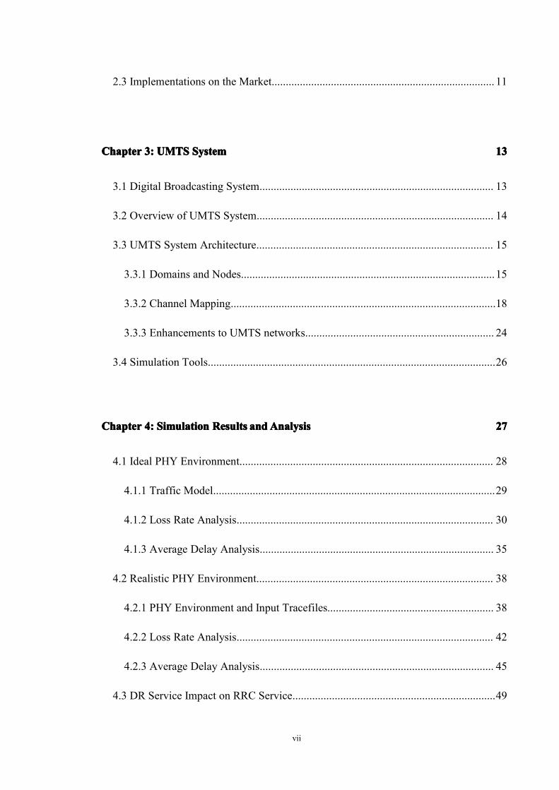
ListListListList ofofofof TablesTablesTablesTables

Table 3.1: Comparison of Digital Broadcasting Systems..................................................14

Table 4.1: Exchange Details of RRC Messages................................................................ 51

Table 4.2: Sizes of RRC Messages with Overheads..........................................................52

Table 4.3: Interval Calculations for One Group................................................................ 55

Table 4.4: Different Packet Sizes and Their Respective Intervals.................................... 57

Table 4.5: Interval Calculations for Two Groups..............................................................61

Table 4.6: Interval Calculations for Three Groups............................................................62

Table 4.7: Confidence Intervals.........................................................................................65

Table 5.1: Comparison of XML Compression Technologies............................................73

x

ListListListList ofofofof FiguresFiguresFiguresFigures

Figure 1.1: An Internet-Based Demand Response System..................................................2

Figure 2.1: User Interface of Programmable Communicating Thermostat......................... 7

Figure 2.2: One-Way Price Event........................................................................................9

Figure 2.3: One-Way Emergency Event............................................................................11

Figure 3.1: UMTS System Architecture............................................................................16

Figure 3.2: Layered Organization......................................................................................19

Figure 3.3: Mapping between Transport Channels and Physical Channels...................... 20

Figure 3.4: Mapping between Logical Channels and Transport Channels........................23

Figure 4.1: Network Topology for Simulations................................................................ 27

Figure 4.2: Loss Rate for TCP-RACH/FACH...................................................................30

Figure 4.3: Loss Rate for UDP-RACH/FACH.................................................................. 31

Figure 4.4: Loss Rate for TCP-DCH/DCH........................................................................32

Figure 4.5: Loss Rate for UDP-DCH/DCH.......................................................................32

Figure 4.6: Loss Rate for TCP-DCH/HS-DSCH...............................................................33

Figure 4.7: Loss Rate for UDP-DCH/HS-DSCH.............................................................. 34

Figure 4.8: Average Delay for TCP-RACH/FACH.......................................................... 35

Figure 4.9: Average Delay for UDP-RACH/FACH..........................................................35

Figure 4.10: Average Delay for TCP-DCH/DCH............................................................. 35

Figure 4.11: Average Delay for UDP-DCH/DCH.............................................................36

Figure 4.12: Average Delay for TCP-DCH/HS-DSCH.....................................................36

xi

Figure 4.13: Average Delay for UDP-DCH/HS-DSCH.................................................... 36

Figure 4.14: Loss Rate for Indoor A Environment............................................................42

Figure 4.15: Loss Rate for Indoor B Environment............................................................ 42

Figure 4.16: Loss Rate for Pedestrian A Environment......................................................43

Figure 4.17: Loss Rate for Pedestrian B Environment...................................................... 43

Figure 4.18: Loss Rate for Urban Environment................................................................ 44

Figure 4.19: Average Delay for Indoor A Environment....................................................45

Figure 4.20: Average Delay for Indoor B Environment....................................................45

Figure 4.21: Average Delay for Pedestrian A Environment..............................................46

Figure 4.22: Average Delay for Pedestrian B Environment..............................................46

Figure 4.23: Average Delay for Urban Environment........................................................ 47

Figure 4.24: RRC Connection Establishment Procedure.................................................. 50

Figure 4.25: RRC Service at Different % of Channel Capacity........................................ 55

Figure 4.26: RRC Service at Different % of Channel Capacity (10%-70%).................... 56

Figure 4.27: RRC Service with DR Service at 10% of Channel Capacity........................ 58

Figure 4.28: RRC Service with or without 10% DR Service (10%-70%).........................58

Figure 4.29: RRC Service with low-frequency DR Service (intervals: 50 Seconds) ......59

Figure 4.30: RRC Service with or without Reasonable DR Service (10%-70%)............. 60

Figure 4.31: RRC Service with or without Reasonable DR Service (Two Groups)......... 63

Figure 4.32: RRC Service with or without Reasonable DR Service (Three Groups)....... 63

Figure 5.1: Pre-Processing Compressor............................................................................ 71

xii

NomenclatureNomenclatureNomenclatureNomenclature

ACK Acknowledgement

AICH Acquisition Indicator Channel

AM Acknowledged Mode

AP-AICH Access Preamble Acquisition Indicator Channel

ARQ Automatic Repeat Request

BCCH Broadcast Control Channel

BCH Broadcast Channel

BS Base Station

BSC Base Station Controller

CAISO California Independent System Operator

CBR Constant Bit Rate

CCCH Common Control Channel

CD/CA-ICH Collision-Detection/Channel-Assignment Indicator Channel

CEC California Energy Commission

CN Core Network

CPCH Uplink Common Packet Channel

CPICH Common Pilot Channel

CQI Channel Quality Indicator

CSICH CPCH Status Indicator Channel

CTCH Common Traffic Channel

xiii

DCCH Dedicated Control Channel

DCH Dedicated Channel

DPCCH Dedicated Physical Control Channel

DPDCH Dedicated Physical Data Channel

DR Demand Response

DSCH Downlink Shared Channel

DTCH Dedicated Traffic Channel

DTD Document Type Definition

ETSI European Telecommunication Standards Institute

EURANE Enhanced UMTS Radio Access Network Extensions for NS-2

FACH Forward Access Channel

FDD Frequency Division Duplex

FM Frequency Modulation

FTP File Transfer Protocol

GGSN Gateway GPRS Support Node

GPRS General Packet Radio Service

GSM Global System for Mobile communication

HFC Hybrid Fiber-Coaxial

HSDPA High Speed Downlink Packet Access

HS-DSCH High Speed Downlink Shared Channel

IE Information Elements

IESO Independent Electricity System Operator

xiv

IM Instant Messaging

IP Internet Protocol

MAC Medium Access Control

ME Mobile Equipment

MS Mobile Station

NS-2 Network Simulator

OPA Ontario Power Authority

PCCH Paging Control Channel

P-CCPCH Primary Common Control Physical Channel

PCH Paging Channel

PCPCH Physical Common Packet Channel

PCT Programmable Communicating Thermostat

PDSCH Physical Downlink Shared Channel

PHY Physical

PICH Paging Indicator Channel

PIER Public Interest Energy Research

PRACH Physical Random Access Channel

PSTN Public Switched Telephone Network

QoS Quality of Service

RACH Random Access Channel

RBDS Radio Broadcast Data System

RLC Radio Link Control

xv

r.m.s. Root Mean Square

RNC Radio Network Controller

RNS Radio Network Subsystem

RRC Radio Resource Control

RRM Radio Resource Management

RTT Round-Trip Time

SAP Service Access Point

SAX Simple API for XML

S-CCPCH Secondary Common Control Physical Channel

SCH Synchronization Channel

SDU Service Data Unit

SEACORN Simulation of Enhanced UMTS Access and Core Networks

SF Spreading Factor

SGSN Serving GPRS Support Node

TCP Transmission Control Protocol

TCP/IP Transmission Control Protocol/Internet Protocol

TDD Time Division Duplex

TM Transparent Mode

UDP User Datagram Protocol

UE User Equipment

UM Unacknowledged Mode

UMTS Universal Mobile Telecommunication System

xvi

USIM UMTS Subscriber Identity Module

UTRAN UMTS Terrestrial Radio Access Network

VoIP Voice-over-IP

W3C World Wide Web Consortium

WCDMA Wideband Code Division Multiple Access

XML Extensible Markup Language

XSD XML Schema Definition

1

ChapterChapterChapterChapter 1:1:1:1: IntroductionIntroductionIntroductionIntroduction

1.1 Overview

In the current Information Age, more and more traditional services are provided

electronically (e.g. mail, banking, shopping, etc). Just like their traditional

counterparts, for such electronic services to fully function, a substantial pre-investment

is always needed, typically in infrastructure. And there are additional costs for

maintaining the infrastructure.

In the past, people built a new system every time a specific new service was required.

This can be very time-consuming and is a waste of resources as many of these services

share the same characteristics. Therefore, a single system that can provide various

services would be beneficial. As the evolution of telecommunication standards and

technologies is ongoing, many cellular systems enable network operators to offer their

customers a variety of services in addition to the traditional voice call.

In this thesis, we will examine how the basic infrastructure associated with the cellular

networks could be applied to the management of a presently unrelated service--

electricity billing and use.

At present, the price per unit of electricity is fixed during the billing period. Power

plant operators have no way to accurately estimate how much each customer will

consume during that time frame, so they always have to be prepared for peak demand.

2

When demand surpasses supply, a power outage can happen, causing financial loss and

affecting people’s daily lives. As shown in Figure 1.1, if the electricity demand can be

estimated dynamically and pre-defined plans are provided for different scenarios, the

probability of electrical blackouts can be greatly reduced. And from the customers’

perspective, their electricity bills can also be reduced as long as they alter their

behaviors accordingly. Demand Response (DR) mechanisms [1] help the operators to

manage demands from the customers in response to supply conditions.

FigureFigureFigureFigure 1.11.11.11.1AnAnAnAn Internet-BasedInternet-BasedInternet-BasedInternet-Based DemandDemandDemandDemand ResponseResponseResponseResponse SystemSystemSystemSystem [2][2][2][2]

By incorporating Demand Response service with the services offered by cellular

networks, the wide coverage of these networks could be exploited. And since this

service would utilize an existing network, no additional cost for infrastructure is

needed.

With the help of the Enhanced UMTS Radio Access Network Extensions for NS-2

3

(EURANE), we have completed a series of simulations using the Network Simulator

(NS-2), and have successfully collected the necessary data to examine the impact of

DR Service on other services within the same network framework as this service would

be incorporated as additional traffic. The methodology is as follows: First, we test all

the transport channels in an ideal physical (PHY) environment, and compare them in

terms of loss rate and average delay. Then we test High Speed Downlink Shared

Channel (HS-DSCH), a new member of the Universal Mobile Telecommunication

System (UMTS), in more realistic PHY environments, generating input tracefiles for

Indoor Office, Pedestrian and Urban area, which are the locations of our potential

customers. Last but not least, the Radio Resource Control (RRC) connection

establishment procedure, which is the essential step before mobile devices access any

service, is modelled by a modified Ping agent. We monitor the behavior of the control

channel after incorporating DR Service to the traffic, and analyze these data as they

reflect the competition of radio resources.

In this thesis, we have proved the following.

� It is feasible to incorporate DR Service to the UMTS framework.

� In ideal PHY environment, if we set aside a separate channel for DR Service,

transport channel pairs RACH/FACH, DCH/DCH and DCH/HS-DSCH are all

capable of delivering desirable service.

� HS-DSCH works well in small cell and low transmit power (Indoor Office and

Pedestrian) environments even without any retransmission mechanism.

4

� When we put DR Service and RRC Service in a shared channel, if the frequency of

DR Service is controlled, its impact on RRC Service is limited.

� XML compression technologies can help to reduce the size of DR messages, and

to minimize the impact DR Service has on RRC Service and network efficiency.

1.2 Outline

The next few chapters are organized like this: Chapter 2 introduces the benefits and a

detailed review of the Programmable Communicating Thermostat (PCT) as an

implementation of DR systems. In Chapter 3, the architecture of the UMTS network

along with the simulator we use are discussed. The simulation results and analysis are

presented in Chapter 4. In Chapter 5, we discuss the possibility of using compression

technologies to control the size of DR messages. We will draw our conclusions in

Chapter 6.

5

ChapterChapterChapterChapter 2222 ReviewReviewReviewReview ofofofof DemandDemandDemandDemand ResponseResponseResponseResponse systemsystemsystemsystem (PCT)(PCT)(PCT)(PCT)

2.1 Background Review

From audio to video, heat to air-conditioning, electrical power plays an irreplaceable

role in people’s daily lives. Electricity comes from different sources. Today we rely

mainly on hydroelectric, coal, natural gas, nuclear and petroleum as well as a small

amount from solar energy, tidal harnesses, wind generators and geothermal sources [3]

[4]. Due to the fact that a large portion of electricity is from non-renewable sources of

energy, its efficiency and distribution are important issues [5] [6].

Electrical power is generated as it is used. And power consumption is highly variable,

both during the year and in the course of a single day. It is very difficult and almost

impossible to store electricity in significant volume or over extended periods of time.

The amount of electricity available is limited by the capacities of power plants (power

stations) [7] [8]. In order to keep up with demand and prevent outages, either more

power plants or extra supply is needed. The first approach requires the construction of

new power stations, which are unnecessary during off-peak hours and incur a

significant cost; the second one uses “backup” sources, i.e. coal, which produce carbon

dioxide (CO2) and contribute to greenhouse gases [9].

Outages happen when the demand load on the power grid exceeds the amount it can

supply and transmit, causing significant consequences. The Northeast Blackout of

6

2003 was the largest power outage in the history of North America. It is estimated that

over 50 million people were affected, including about 10 million in the province of

Ontario (about one third of the population of Canada) and 40 million in eight U.S.

states (about one seventh of the population of the U.S.). And the related financial losses

were estimated at $6 billion USD [10] [11].

2.2 Programmable Communicating Thermostat

Demand response technology allows energy customers the ability to modify their

electricity consumption patterns in response to constantly fluctuating energy prices or

to emergency curtailment requests. This can greatly reduce the possibility of

widespread power outages [12]. The Programmable Communicating Thermostat (PCT)

from the California Energy Commission (CEC) is one example [13]. It is motivated by

a need to prevent blackouts and also to provide overall lower rates for customers [14].

The PCT allows customers to manage the cost of their electricity consumption, which

is defined to be a "price event".

The most significant feature of the PCT is its ability to perform automatic temperature

control as demand approaches maximum supply, which is an "emergency event".

Just like phone numbers are used to identify mobile users in a cellular system, every

PCT can be explicitly addressed by its coverage area, substation, utility and demand

response (DR) program. All the PCTs in a neighborhood periodically receive messages

from a central DR system. This constitutes a one-way communication system by

7

default, whereby the central DR system issues messages to inform customers about

price events and emergency events. When the PCTs receive these messages, they

follow the instructions to perform temporary temperature control.

FigureFigureFigureFigure 2.12.12.12.1 UserUserUserUser InterfaceInterfaceInterfaceInterface ofofofof ProgrammableProgrammableProgrammableProgrammable CommunicatingCommunicatingCommunicatingCommunicating ThermostatThermostatThermostatThermostat [14][14][14][14]

As shown in Figure 2.1, each device has an LCD monitor to display information like

the current temperature, type of event in process, communication status and thermostat

setting, etc. Customers can change the thermostat setting at any point, but depending

on supply conditions, these settings may not go into effect immediately.

Every device is also equipped with a sensor to detect the current temperature. A clock

mechanism makes sure the PCTs are synchronized with the central DR system, so that

they can execute temperature setpoints that are pre-scheduled by customers, as well as

respond to different types of events managed by the central DR system.

Typically, the PCTs are programmed to function according to four periods (morning,

day, evening and night) during a 24-hour day. A weekday and weekend (5-2) schedule

8

is also supported. Distinct daily periods and weekly schedules can be set for heating,

cooling and dual mode.

2.2.1 Normal Mode

The PCTs can work under three different operation modes. The Normal Mode is

designed to be the main operation mode. It determines how the PCT operates in the

absence of price events and emergency events. Customers are able to define the daily

periods and weekly schedules, the temperature setpoints with their associated time

frames, and the temperature offsets for both heating and cooling, which determine the

number of degrees to be adjusted when events happen.

Other than the Normal Mode, there are two basic event operation modes. One is the

Price Event Mode, which is optional and can be overridden by customers. The other is

the Emergency Event Mode, which can override any other modes and can force an

involuntary reduction in load.

2.2.2 Price Event Mode

The central DR system is designed to manage overall demand by first motivating

households to reduce consumption on a voluntary basis when supply becomes tight,

9

and then to impose mandatory temperature adjustments if supply becomes depleted.

When the energy supply becomes tight, yet has not overwhelmed the energy demand, a

price event message is issued. In Figure 2.2, the central DR system simply broadcasts

this message to indicate that a peak price goes into effect soon and provides the details

of this event: the start and stop time (duration), and the explicit price.

Upon receiving this message, the PCT’ response is to increase (for cooling) or

decrease (for heating) the current temperature setpoint by the number of degrees

defined in the temperature offset to lower the energy usage for the duration of the event.

But customers are also allowed to override individual price events whenever they

want if they do not care about cost. Instead of accepting the recommended instructions

and changing their behaviors, they can stick to their routines and pay higher electricity

bills.

FigureFigureFigureFigure 2.22.22.22.2 One-WayOne-WayOne-WayOne-Way PricePricePricePrice EventEventEventEvent [14][14][14][14]

10

2.2.3 Emergency Event Mode

When the electricity reserve is extremely low, voluntary curtailment may not be

enough to alleviate the situation. In Figure 2.3, an emergency event message is issued

to indicate that a more substantial reduction is needed.

At stage 1 of emergency events, the central DR system addresses the grid reliability

situation to all PCTs and specifies an arbitrary offset or a specific setpoint, customers'

allowable choices on temperature are restricted to a narrower range. In essence, this is

no more than a price event since customers still have control over the current

temperature setpoint. However, it provides a chance to mitigate the situation.

If the grid is still in urgent condition, at stage 2, the central DR system will impose an

offset or a setpoint on every PCT. No matter whether customers are willing or not, their

PCTs must comply with these commands. All customer-initiated changes to the

thermostat setting are suspended until the emergency event is completed.

11

FigureFigureFigureFigure 2.32.32.32.3 One-WayOne-WayOne-WayOne-Way EmergencyEmergencyEmergencyEmergency EventEventEventEvent [14][14][14][14]

Both price events and emergency events last for a specified period of time, as indicated

in their respective messages. When an event is prematurely terminated, or the event

expires before another one goes into effect, the PCT will return to the Normal Mode.

2.3 Implementations on the Market

Preventing blackouts is not the sole rationale for DR systems, many proposals have

existed long before blackouts began to happen. Other rationales would be to better

manage peak demand, and to possibly control widespread population demand in order

to mitigate climate change.

Today, some technologies are already available and more are under development in

12

order to automate the demand response system. In the United States, GridWise [15]

and EnergyWeb [16] are the two major federal initiatives to develop and promote these

technologies nationwide. In California, the California Independent System Operator

(CAISO) [17], a non-profit public corporation, is responsible for operating the

majority of the state’s high-voltage wholesale power grid, avoiding rotating brownouts

and ensuring qualified households access to the electricity grid. The California Energy

Commission’s Public Interest Energy Research (PIER) [18] program brought demand

response services to the marketplace and created statewide environmental and

economic benefits. In Canada, the Independent Electricity System Operator (IESO) [19]

is in charge of balancing both the supply and demand for electricity in Ontario and

directing its flow across the province’s transmission lines. Ontario Power Authority

(OPA) [20] and Toronto Hydro Corporation [21] are also working on services aimed at

consumers.

13

ChapterChapterChapterChapter 3333 UMTSUMTSUMTSUMTS SystemSystemSystemSystem

3.1 Digital Broadcasting Systems

Our research is on the communication interface connecting end-devices in residential

homes to the central DR system. This can be done by either starting from scratch or

choosing an existing system and piggybacking these messages onto a channel already

in use. As shown in Table 3.1, currently, there are many platforms available that can be

used for our project. Each of them has their own advantages and disadvantages. In this

case, one that can balance the tradeoffs is suitable.

Since this is for residential access, the hybrid fiber-coaxial (HFC) network [22] is an

obvious choice as it is commonly employed by cable TV operators. In order to

implement an application like this, these messages can be carried on radio frequency

signals without incurring any additional cost. The problem is that the HFC network is

wired and therefore the flexibility is strictly limited as the PCTs are supposed to be in

or near the kitchen. The Internet-based system is another similar choice. These

messages are sent to customers as alerts. The bandwidth they consume is negligible.

There are already some Internet-based applications on the market, but they require

manual operation and have the same problem as the HFC network since not every

home has Internet, let alone wireless connection.

On the contrary, radio networks have almost ubiquitous coverage and hence provide

14

great accessibility. In fact, one of the wide-area communications systems that the PCT

uses is the Radio Broadcast Data System (RBDS), which can send small amounts of

digital information using conventional FM radio.

The company that motivates this project has 3G infrastructure for us to implement this

system on top of a UMTS network out of all candidates, which also provides good

coverage.

TableTableTableTable 3.13.13.13.1 ComparisonComparisonComparisonComparison ofofofof DigitalDigitalDigitalDigital BroadcastingBroadcastingBroadcastingBroadcasting SystemsSystemsSystemsSystems

3.2 Overview of UMTS System

Over the last several decades, cellular networks have evolved considerably. In the

analog cellular age, they carry only speech [23]; after that, digital cellular systems like

GPRS (General Packet Radio Service) [24] can also carry packet switched data and

support various types of applications such as Instant Messaging (IM), email, etc; now

we are in the high speed age, the emphasis is on integrating all kinds of services like

web access, file transfer and video telephony with the traditional voice-only service.

GSM (Global System for Mobile Communications) [25] [26], which provides digital

call quality in both signaling and speech channels, is considered as a second generation

(2G) [27] mobile phone system. However, it is still a pure circuit switched service.

Coverage Communication Cost

Cable/Internet Limited Minimal

Radio network Wide Minimal

UMTS Wide Minimal

15

2.5G is a stepping stone between 2G and 3G. Even though the term is not officially

defined, it is used to describe 2G systems that have implemented an additional packet

switched domain. GPRS is a 2.5G technology used by GSM operators. It provides data

rates from 56 kbps to 114 kbps.

The cellular networks are now heading towards an all-IP based network and it is likely

that in the future all services will be made available over IP. The third generation (3G)

[28] systems support high-speed packet switched data (up to 2Mbps) and they are the

next step beyond GPRS.

Currently the 3G cellular systems are being evolved from the existing cellular

networks. Being promoted by ETSI (European Telecommunication Standards Institute)

[29], UMTS (Universal Mobile Telecommunication System) [30] is one that provides

a vital link between today's multiple GSM systems. It is used as the platform for our

task.

3.3 UMTS System Architecture

3.3.1 Domains and Nodes

As shown in Figure 3.1, the UMTS system is composed of three distinct domains:

Core Network (CN), UMTS Terrestrial Radio Access Network (UTRAN) and User

Equipment (UE). Entities in the system interact with each other via different interfaces.

16

FigureFigureFigureFigure 3.13.13.13.1 UMTSUMTSUMTSUMTS SystemSystemSystemSystemArchitectureArchitectureArchitectureArchitecture

The CN is the centralized part of the UMTS system. It is subdivided into a circuit-

switched and a packet-switched domain. Interesting elements in the latter domain are

Serving GPRS Support Node (SGSN) and Gateway GPRS Support Node (GGSN). The

SGSN serves as a gateway between the CN and the UTRAN, and is in charge of

delivering data packets from or to the UTRAN within a certain geographical area. The

GGSN’s job is format and address conversion of data packets between the UMTS

system and external networks. Being connected to these external networks (e.g.

Internet, PSTN), the CN provides switching, routing and forwarding of user traffic and

also contains some network management functions.

UTRAN, which uses Wideband Code Division Multiple Access (WCDMA)

technology, is the new underlying radio interface for the UMTS system. Its function is

to provide air interface access for UEs. WCDMA can operate in two basic modes:

Time Division Duplex (TDD) and Frequency Division Duplex (FDD). In UTRAN, the

17

Base Station (BS) is referred to as Node-B and can serve one or more cells. A set of

Node-Bs is controlled by an equipment called Radio Network Controller (RNC). One

RNC and its associated Node-Bs form a Radio Network Subsystem (RNS). The

UTRAN consists of several such RNSs.

As the governing element in the UTRAN, RNC performs the same functions as the

Base Station Controller (BSC) in GSM and thus is responsible for managing both radio

and terrestrial channels. It also carries out Radio Resource Management (RRM) to

control the co-channel interference and other radio transmission characteristics (e.g.

transmit power, modulation scheme, error coding scheme).

The Node-B, which is the counterpart of a BS in GSM, is the physical unit for the

transmission/reception of radio signals within the cells. Traditionally, most functions

are performed at the RNC, whereas the Node-B has limited functionality. However,

with the emergence of High Speed Downlink Packet Access (HSDPA), some

functionality (e.g. retransmission) is moved and now handled by the Node-B to lower

response times. This will be further discussed in the simulations.

The UE is based on the same principles as the Mobile Station (MS) in GSM. Mobile

Equipment (ME) and UMTS subscriber identity module (USIM) card are separated

from each other [31] [32]. The UEs represent the end-devices in our task. They receive

both price and emergency event messages and respond accordingly.

18

3.3.2 Channel Mapping

For the channel organization, the UMTS system is three-layered, as presented in

Figure 3.2. Like every other layering approach, it provides convenience to ensure

effective control of multiplexing. At the lowest layer, the PHY layer provides the

means of transmitting raw bits and offers services to the immediately above MAC

layer in the form of transport channels. The MAC layer provides hardware addressing

and channel access mechanisms and it in turn offers services to the RLC layer via

logical channels. The RLC layer is in charge of handling user data and offering

services to higher layers through SAPs, which are used to distinguish between

different applications.

19

FigureFigureFigureFigure 3.23.23.23.2 LayeredLayeredLayeredLayeredOrganizationOrganizationOrganizationOrganization

Since services are provided via channels and the mappings between channels happen in

the lower two layers, we review this layered architecture in a bottom-up manner.

Physical Layer

The whole point of the 3G system is to support various services (mainly wideband

20

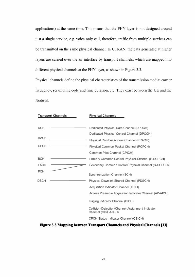
applications) at the same time. This means that the PHY layer is not designed around

just a single service, e.g. voice-only call, therefore, traffic from multiple services can

be transmitted on the same physical channel. In UTRAN, the data generated at higher

layers are carried over the air interface by transport channels, which are mapped into

different physical channels at the PHY layer, as shown in Figure 3.3.

Physical channels define the physical characteristics of the transmission media: carrier

frequency, scrambling code and time duration, etc. They exist between the UE and the

Node-B.

FigureFigureFigureFigure 3.33.33.33.3 MappingMappingMappingMapping betweenbetweenbetweenbetweenTransportTransportTransportTransport ChannelsChannelsChannelsChannels andandandand PhysicalPhysicalPhysicalPhysical ChannelsChannelsChannelsChannels [3[3[3[33333]]]]

21

Because of different QoS requirements, two types of transport channels are designed

to meet various needs: dedicated channels and common channels. As the name

indicates, in a dedicated channel, the whole resources, which are identified by a certain

code on a certain frequency, are reserved for a single user in the cell. On the contrary,

in a common channel, resources are divided among all or a group of users, thus

concurrent traffic can exist in the same link.

The only dedicated transport channel is the dedicated channel (DCH). On the other

hand, currently six different common transport channels are defined in UTRAN. They

are the Broadcast Channel (BCH), Forward Access Channel (FACH), Random Access

Channel (RACH), Paging Channel (PCH), Uplink Common Packet Channel (CPCH)

and the Downlink Shared Channel (DSCH).

BCH is used for broadcasting system information into an entire cell. RACH/FACH is a

transport channel pair that carries control information to or from the terminals. FACH

is the downlink and RACH is the uplink. They are usually used for connection

establishment (control information). They can also be used to transmit user data, but

the bit rates are strictly limited. PCH comes into play when the network wants to

initiate communication with a terminal, it is a downlink transport channel that carries

data relevant to the paging procedure. CPCH is for the transmission of bursty data

traffic in the uplink direction. Also providing transport support in the downlink

direction is DSCH, which carries user data and/or control information and can be

shared by several users. The common transport channels needed for the basic network

operation are FACH, RACH and PCH, while the use of BCH, DSCH and CPCH is

22

optional and can be decided by the network.

Medium Access Control Protocol

The transport and logical channels define what type of data are transferred, thus more

functionalities are involved. The Medium Access Control (MAC) protocol is active at

UE and the RNC.

The data transfer services of the MAC layer are provided by the logical channels.

Different types of data services require different logical channels. The logical channels

can be classified into two groups: Control Channels, which are used to transfer control

information; Traffic Channels, which are used for user information. The mapping

between logical channels and transport channels are presented in Figure 3.4.

The Control Channels are:

1. Dedicated Control Channel (DCCH): An exclusive bidirectional channel that

transmits dedicated control information between a specific UE and the network.

2. Common Control Channel (CCCH): A bidirectional channel shared by many UEs,

transmitting control information between them and the network.

3. Broadcast Control Channel (BCCH). A downlink channel for broadcasting system

control information.

4. Paging Control Channel (PCCH). A downlink channel that transfers paging

information.

The Traffic Channels are:

23

1. Dedicated Traffic Channel (DTCH). A bidirectional channel dedicated to one

specific UE, transferring user information.

2. Common Traffic Channel (CTCH). A downlink channel for all or a group of UEs,

transferring user information.

FigureFigureFigureFigure 3.43.43.43.4 MappingMappingMappingMapping betweenbetweenbetweenbetweenLogicalLogicalLogicalLogicalChannelsChannelsChannelsChannels andandandandTransportTransportTransportTransport ChannelsChannelsChannelsChannels [3[3[3[33333]]]]

Radio Link Control Protocol

The Radio Link Control (RLC) protocol also runs in both the UE and the RNC. It

implements the Data Link Layer (Link Layer) functionality over the WCDMA

interface. It provides segmentation and flow control services, among others, for both

control and user data. Based on different requirements, mainly error recovery

(retransmission), every RLC instance is configured to operate in one of three modes:

Acknowledged Mode (AM), Unacknowledged Mode (UM) or Transparent Mode (TM).

In the Acknowledged Mode (AM), error correction is handled by an automatic repeat

request (ARQ) mechanism. However, when the maximum number of retransmissions

24

is reached or the transmission time is exceeded, the delivery is considered as an

unsuccessful one. The Service Data Unit (SDU) would be discarded and the peer entity

on the other end would be informed. The AM entity is defined to be bidirectional and

can piggyback the link status onto user data in the opposite direction. The AM is

normally the choice for packet-type services, e.g. web browsing and email.

In the Unacknowledged Mode (UM), no retransmission protocol is implemented and

thus data delivery is not guaranteed. Received corrupted data is either marked

erroneous or discarded depending on the configuration. The UM entity is defined as

unidirectional. Since the link status is not necessary, an association between the uplink

and downlink is not needed. It is usually used by loss-tolerant applications, e.g. Voice-

over-IP (VoIP).

The Transparent Mode (TM) is just like UM except that it offers a circuit-switched

service instead of a packet-switched service [33] [34].

3.3.3 Enhancements to UMTS Networks

In the UMTS release 99 [35], with Code Division Multiple Access (CDMA)

incorporated as the air interface, the first UMTS 3G networks are specified. Three

downlink transport channels are defined: Dedicated Channel (DCH), Forward Access

Channel (FACH), Downlink Shared Channel (DSCH).

In CDMA, different codes are used to distinguish different connections (users). The

Spreading Factor (SF), which defines the number of available codes, is fixed for DCH.

25

And because distinct users take turns to access the resources in a dedicated channel,

individual users may reserve codes when they do not necessarily need them.

This contributes to a slow channel reconfiguration process, thus affecting the

efficiency of DCH for high rate and bursty services. FACH is typically used for small

amounts of data, it is not capable of offering high rate and bursty services either. In

DSCH, it is possible to time-multiplex different users at the same time. And with a fast

channel reconfiguration process and a packet scheduling mechanism, it works

significantly more efficient than DCH.

HSDPA is targeted at increasing the peak data rate and throughput, reducing the delay,

and improving the spectral efficiency of the downlink. It further develops DSCH, in

the form of High Speed Downlink Shared Channel (HS-DSCH), and transfers some of

the MAC functionalities from the RNC to the BS.

HS-DSCH introduces some new features, the most interesting one is Hybrid ARQ with

soft combining. Hybrid ARQ not only can detect, but also can correct a corrupted

packet with some additional bits. And incorrectly received packets are stored at the

receiver rather than discarded, and can be combined with following retransmissions to

increase the probability of successful decoding.

Hybrid ARQ performs better than ARQ in poor signal conditions, thus is very

important for wireless channels. And it allows the UMTS system to offer enhanced

services [40].

26

3.4 Simulation Tools

Network Simulator (NS-2) [37] is an event-driven simulator which has been widely

used in the academic community. It is open-source, object-oriented and suitable for

simulation of traffic behaviors, network (both wired and wireless) protocols, etc.

However, NS-2 is a network (TCP/IP) simulator in nature. It has highly detailed and

hardcoded concepts about nodes, links, agents, protocols, packet representations and

network addresses, etc. Thus, it is almost impossible to simulate things other than

packet-switching networks and protocols solely with it. Owing to the fact that the PHY

and MAC layers are not detailed enough, an extension which can complement the

lower layers is essential.

The EURANE (Enhanced UMTS Radio Access Network Extensions for NS-2) [38] is

developed within the framework of the IST SEACORN [39] project. This extension

limits the simulations to one cell, so that no handover is implemented. It includes three

additional nodes (RNC, BS and UE), their functionality allow for the support of these

transport channels: FACH, RACH, DCH and HS-DSCH. Our simulation model uses

the Application, Transport and Network layer functionality provided by NS-2 and the

EURANE extension provides the MAC and PHY layer support.

27

ChapterChapterChapterChapter 4444 SimulationSimulationSimulationSimulationResultsResultsResultsResults andandandandAnalysisAnalysisAnalysisAnalysis

FigureFigureFigureFigure 4.14.14.14.1 NetworkNetworkNetworkNetwork TopologyTopologyTopologyTopology forforforfor SimulationsSimulationsSimulationsSimulations

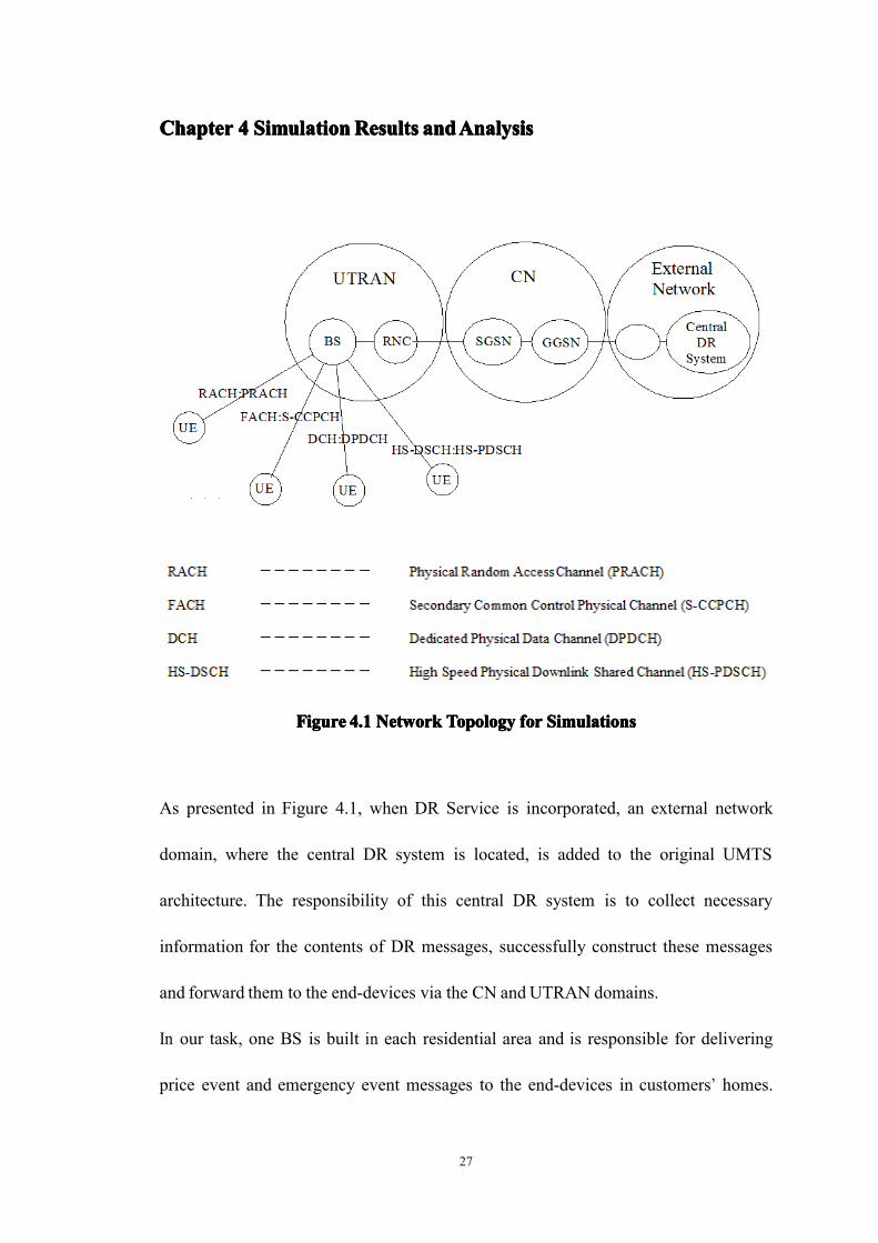
As presented in Figure 4.1, when DR Service is incorporated, an external network

domain, where the central DR system is located, is added to the original UMTS

architecture. The responsibility of this central DR system is to collect necessary

information for the contents of DR messages, successfully construct these messages

and forward them to the end-devices via the CN and UTRAN domains.

In our task, one BS is built in each residential area and is responsible for delivering

price event and emergency event messages to the end-devices in customers’ homes.

28

Since we only consider single-cell scenarios, one RNC is also included in the UTRAN.

In practice, a single RNC is in charge of managing multiple BSs.

We also have a SGSN node as the gateway, it connects the RNC with the GGSN. The

GGSN is further linked to anther two nodes in the external network. The central DR

system is located at the second node.

4.1 Ideal PHY Environment

The EURANE extension offers support of four different transport channels: FACH,

RACH, DCH and HS-DSCH, and they can be formed as three two-way transport

channel pairs [40]:

FACH/RACH: both are common channels, FACH is the downlink channel and RACH

is the uplink channel

DCH/DCH: DCH is a dedicated channel and it can operate in both the downlink and

the uplink

HS-DSCH/DCH: HS-DSCH is a downlink channel and an associated DCH is always

needed as the uplink channel

Each transport channel pair provides different Quality of Service (QoS) for different

types of control or user data. This part of our simulations is to find out how these

transport channel pairs behave in an ideal PHY environment.

29

4.1.1 Traffic Model

We use 20 UEs for our simulation, each individual UE represents a group of customers

in real life and the traffic from one UE is considered as the aggregate traffic from the

customers in that particular group. The number of UEs is only restrained by the

computer’s memory capacity. 20 is a reasonable choice because increasing this number

does not necessarily increase the accuracy and 20 is large enough to give us relatively

accurate results.

Both transport layer protocols (TCP and UDP) are used, along with the three transport

channel pairs, to create six different combinations: TCP-RACH/FACH, UDP-

RACH/FACH, TCP-DCH/DCH, UDP-DCH/DCH, TCP-DCH/HS-DSCH, UDP-

DCH/HS-DSCH. Note our goal here is to find out which combination can perform best

in the ideal PHY environment, even though TCP cases are never considered in practice

and are only included as comparisons. Since DR messages are broadcast on a regular

basis, reliable and connection-oriented service is not needed.

We use AM mode at the RLC layer to make sure that the reliable service from the

lower layers provides a fair platform for the transport layer. Thus, packets can only get

lost when transmitting over the wired link, if they get lost at all.

The packet size is 150 bytes, which includes both TCP/UDP and IP overheads. In this

simulation model, the size of all packets is fixed and the default value is 40 bytes, with

larger packets being converted into multiple smaller packets, e.g., one 150-byte packet

equals four 40-byte packets.

30

In order to generate user data, TCP uses File Transport Protocol (FTP) generator,

which represents a bulk data transfer of large size. The FTP generator does not have

any interval or rate parameter, however, the TCP window size is changed to 1, which

means as soon as a packet is generated, it gets transferred immediately.

In UDP's case, a Constant Bit Rate (CBR) traffic source is used for generating one 150-

byte packet every 2 seconds.

The idealtrace, which is an input tracefiles that does not have any errors and uses a

fixed Channel Quality Indicator (CQI) value, is used for this set of simulations. It is for

creating an ideal PHY environment where no radio effects are added to the channel.

4.1.2 Loss Rate Analysis

Loss rate for TCP-RACH/FACHLoss rate for TCP-RACH/FACHLoss rate for TCP-RACH/FACHLoss rate for TCP-RACH/FACH

0000200200200200400400400400600600600600800800800800

1000100010001000

UE(0)UE(0)UE(0)UE(0)





UE(10)

UE(10)

UE(10)

UE(10)

UE(12)

UE(12)

UE(12)

UE(12)

UE(14)

UE(14)

UE(14)

UE(14)

UE(16)

UE(16)

UE(16)

UE(16)

UE(18)

UE(18)

UE(18)

UE(18)

Received PacketsReceived PacketsReceived PacketsReceived PacketsLost PacketsLost PacketsLost PacketsLost Packets

FigureFigureFigureFigure 4.4.4.4.2222 LossLossLossLossRateRateRateRate forforforfor TCP-RACH/FACHTCP-RACH/FACHTCP-RACH/FACHTCP-RACH/FACH

In Figure 4.2, for the TCP-RACH/FACH scenario, each UE receives about 550-650

packets in the end and loses about 750-850 packets during the process.

31

Loss rate for UDP-RACH/FACHLoss rate for UDP-RACH/FACHLoss rate for UDP-RACH/FACHLoss rate for UDP-RACH/FACH

0000101010102020202030303030404040405050505060606060






UE(10)

UE(10)

UE(10)

UE(10)

UE(12)

UE(12)

UE(12)

UE(12)

UE(14)

UE(14)

UE(14)

UE(14)

UE(16)

UE(16)

UE(16)

UE(16)

UE(18)

UE(18)

UE(18)

UE(18)


FigureFigureFigureFigure 4.4.4.4.3333 LossLossLossLossRateRateRateRate forforforfor UDP-RACH/FACHUDP-RACH/FACHUDP-RACH/FACHUDP-RACH/FACH

In Figure 4.3, for the UDP-RACH/FACH scenario, each UE receives exact 50 packets

in the end and loses about 30-40 packets during the process. The AM mode makes sure

the number of transmitted packets is always equal to the number of received packets.

But packets are still subject to radio effects, e.g. fading, shadowing, channel congestion

and potential PHY layer impairments, they are not exempt from getting lost. As long as

a packet is not correctly received, it counts as a lost one. Multiple lost packets may

even be the corrupt copies of the same packet.

Because of the idealtrace, there should not be any PHY layer impairments. FACH is

the downlink half of the common channel pair and is capable of supporting multiple

users at the same time, however, it is usually used for small quantities of data, even for

this relatively moderate traffic, many packets are dropped because of congestion.

32

Loss rate for TCP-DCH/DCHLoss rate for TCP-DCH/DCHLoss rate for TCP-DCH/DCHLoss rate for TCP-DCH/DCH

00002000200020002000400040004000400060006000600060008000800080008000

10000100001000010000






UE(10)

UE(10)

UE(10)

UE(10)

UE(12)

UE(12)

UE(12)

UE(12)

UE(14)

UE(14)

UE(14)

UE(14)

UE(16)

UE(16)

UE(16)

UE(16)

UE(18)

UE(18)

UE(18)

UE(18)


FigureFigureFigureFigure 4.4.4.4.4444 LossLossLossLossRateRateRateRate forforforfor TCP-DCH/DCHTCP-DCH/DCHTCP-DCH/DCHTCP-DCH/DCH

In Figure 4.4, for the TCP-DCH/DCH scenario, each UE receives about 8200 packets

in the end and no packet is lost during the process. Compared to the TCP-RACH/FACH

scenario, a lot more packets are transmitted in this scenario. Because the traffic source

is bulk data of relatively large size (150 bytes), the chance is that two or even more

connections access the shared channel (FACH) at any given time, thus the effective

data rate for each individual connection is reduced. On the other hand, DCH is capable

of supporting traffic at this rate.

Loss rate for UDP-DCH/DCHLoss rate for UDP-DCH/DCHLoss rate for UDP-DCH/DCHLoss rate for UDP-DCH/DCH

0000101010102020202030303030404040405050505060606060






UE(10)

UE(10)

UE(10)

UE(10)

UE(12)

UE(12)

UE(12)

UE(12)

UE(14)

UE(14)

UE(14)

UE(14)

UE(16)

UE(16)

UE(16)

UE(16)

UE(18)

UE(18)

UE(18)

UE(18)


FigureFigureFigureFigure 4.4.4.4.5555 LossLossLossLossRateRateRateRate forforforfor UDP-DCH/DCHUDP-DCH/DCHUDP-DCH/DCHUDP-DCH/DCH

In Figure 4.5, for the UDP-DCH/DCH scenario, each UE receives exact 50 packets in

the end and no packet is lost during the process.

33

With a low data rate and a small packet size (150 bytes), individual users can finish

their transmission within their allocated time slots, and leave no effects on the next

users. DCH is able to recover from switching from one user to another, thus the chance

of losing packets is slim.

Loss rate for TCP-DCH/HS-DSCHLoss rate for TCP-DCH/HS-DSCHLoss rate for TCP-DCH/HS-DSCHLoss rate for TCP-DCH/HS-DSCH

0000500500500500

10001000100010001500150015001500200020002000200025002500250025003000300030003000






UE(10)

UE(10)

UE(10)

UE(10)

UE(12)

UE(12)

UE(12)

UE(12)

UE(14)

UE(14)

UE(14)

UE(14)

UE(16)

UE(16)

UE(16)

UE(16)

UE(18)

UE(18)

UE(18)

UE(18)


FigureFigureFigureFigure 4.4.4.4.6666 LossLossLossLossRateRateRateRate forforforfor TCP-DCH/HS-DSCHTCP-DCH/HS-DSCHTCP-DCH/HS-DSCHTCP-DCH/HS-DSCH

In Figure 4.6, for the TCP-DCH/HS-DSCH scenario, each UE receives about 2800

packets in the end and no packet is lost during the process. However, this is merely 1/3

of the throughput of the TCP-DCH/DCH scenario.

As mentioned above, packet scheduling mechanism is moved from RNC to Node-B in

HSDPA, i.e., RNC handles packet scheduling for RACH, FACH and DCH, and Node-

B takes care of HS-DSCH. When it comes to high throughput applications, HS-DSCH

provides better performance since it reacts faster to varying channel condition.

For dedicated channel traffic, a fixed bandwidth is reserved for each connection. But

for HS-DSCH, this is not efficient because air interface throughput is higher and more

variable. The traffic scheduling can cause a change in resource allocation, thus the data

rate may not be consistent during a connection, and HS-DSCH traffic does not

34

necessarily have a higher throughput [41].

Loss rate for UDP-DCH/HS-DSCHLoss rate for UDP-DCH/HS-DSCHLoss rate for UDP-DCH/HS-DSCHLoss rate for UDP-DCH/HS-DSCH

0000101010102020202030303030404040405050505060606060






UE(10)

UE(10)

UE(10)

UE(10)

UE(12)

UE(12)

UE(12)

UE(12)

UE(14)

UE(14)

UE(14)

UE(14)

UE(16)

UE(16)

UE(16)

UE(16)

UE(18)

UE(18)

UE(18)

UE(18)


FigureFigureFigureFigure 4.4.4.4.7777 LossLossLossLossRateRateRateRate forforforfor UDP-DCH/HS-DSCHUDP-DCH/HS-DSCHUDP-DCH/HS-DSCHUDP-DCH/HS-DSCH

In Figure 4.7, for the UDP-DCH/HS-DSCH scenario, each UE receives exact 50

packets in the end and no packet is lost during the process.

In terms of loss rate, the HS-DSCH also performs well.

Summary:

� The results for the UDP cases are consistent with what we have set up.

� For wireless system, limited resources such as link bandwidth are allocated for

active users on demand. The bandwidth available to a single user can be affected

by various factors, e.g., changing link rate or scheduling algorithm of shared

resources. In TCP’s case, using different transport channels, UEs receive different

numbers of packets.

35

4.1.3 Average Delay Analysis

The unit for average delay is second.

Average delay for TCP-RACH/FACHAverage delay for TCP-RACH/FACHAverage delay for TCP-RACH/FACHAverage delay for TCP-RACH/FACH

0000

0.40.40.40.40.80.80.80.8

1.21.21.21.2

1.61.61.61.6






UE(10)

UE(10)

UE(10)

UE(10)

UE(12)

UE(12)

UE(12)

UE(12)

UE(14)

UE(14)

UE(14)

UE(14)

UE(16)

UE(16)

UE(16)

UE(16)

UE(18)

UE(18)

UE(18)

UE(18)

FigureFigureFigureFigure 4.4.4.4.8888AverageAverageAverageAverageDelayDelayDelayDelay forforforfor TCP-RACH/FACHTCP-RACH/FACHTCP-RACH/FACHTCP-RACH/FACH

Average delay for UDP-RACH/FACHAverage delay for UDP-RACH/FACHAverage delay for UDP-RACH/FACHAverage delay for UDP-RACH/FACH

0000

0.10.10.10.1

0.20.20.20.2

0.30.30.30.3






UE(10)

UE(10)

UE(10)

UE(10)

UE(12)

UE(12)

UE(12)

UE(12)

UE(14)

UE(14)

UE(14)

UE(14)

UE(16)

UE(16)

UE(16)

UE(16)

UE(18)

UE(18)

UE(18)

UE(18)

FigureFigureFigureFigure 4.4.4.4.9999AverageAverageAverageAverageDelayDelayDelayDelay forforforfor UDP-RACH/FACHUDP-RACH/FACHUDP-RACH/FACHUDP-RACH/FACH

Average delay for TCP-DCH/DCHAverage delay for TCP-DCH/DCHAverage delay for TCP-DCH/DCHAverage delay for TCP-DCH/DCH

00000.060.060.060.060.120.120.120.12

0.180.180.180.180.240.240.240.24






UE(10)

UE(10)

UE(10)

UE(10)

UE(12)

UE(12)

UE(12)

UE(12)

UE(14)

UE(14)

UE(14)

UE(14)

UE(16)

UE(16)

UE(16)

UE(16)

UE(18)

UE(18)

UE(18)

UE(18)

FigureFigureFigureFigure 4.4.4.4.10101010AverageAverageAverageAverageDelayDelayDelayDelay forforforfor TCP-DCH/DCHTCP-DCH/DCHTCP-DCH/DCHTCP-DCH/DCH

36

Average delay for UDP-DCH/DCHAverage delay for UDP-DCH/DCHAverage delay for UDP-DCH/DCHAverage delay for UDP-DCH/DCH

0000

0.050.050.050.05

0.10.10.10.1

0.150.150.150.15






UE(10)

UE(10)

UE(10)

UE(10)

UE(12)

UE(12)

UE(12)

UE(12)

UE(14)

UE(14)

UE(14)

UE(14)

UE(16)

UE(16)

UE(16)

UE(16)

UE(18)

UE(18)

UE(18)

UE(18)

FigureFigureFigureFigure 4.14.14.14.11111AverageAverageAverageAverageDelayDelayDelayDelay forforforfor UDP-DCH/DCHUDP-DCH/DCHUDP-DCH/DCHUDP-DCH/DCH

Average delay for TCP-DCH/HS-DSCHAverage delay for TCP-DCH/HS-DSCHAverage delay for TCP-DCH/HS-DSCHAverage delay for TCP-DCH/HS-DSCH

00000.040.040.040.040.080.080.080.08

0.120.120.120.120.160.160.160.16






UE(10)

UE(10)

UE(10)

UE(10)

UE(12)

UE(12)

UE(12)

UE(12)

UE(14)

UE(14)

UE(14)

UE(14)

UE(16)

UE(16)

UE(16)

UE(16)

UE(18)

UE(18)

UE(18)

UE(18)

FigureFigureFigureFigure 4.14.14.14.12222AverageAverageAverageAverageDelayDelayDelayDelay forforforfor TCP-DCH/HS-DSCHTCP-DCH/HS-DSCHTCP-DCH/HS-DSCHTCP-DCH/HS-DSCH

Average delay for UDP-DCH/HS-DSCHAverage delay for UDP-DCH/HS-DSCHAverage delay for UDP-DCH/HS-DSCHAverage delay for UDP-DCH/HS-DSCH

00000.040.040.040.040.080.080.080.08

0.120.120.120.120.160.160.160.16






UE(10)

UE(10)

UE(10)

UE(10)

UE(12)

UE(12)

UE(12)

UE(12)

UE(14)

UE(14)

UE(14)

UE(14)

UE(16)

UE(16)

UE(16)

UE(16)

UE(18)

UE(18)

UE(18)

UE(18)

FigureFigureFigureFigure 4.14.14.14.13333AverageAverageAverageAverageDelayDelayDelayDelay forforforfor UDP-DCH/HS-DSCHUDP-DCH/HS-DSCHUDP-DCH/HS-DSCHUDP-DCH/HS-DSCH

37

Summary:

As presented in Figure 4.8--Figure 4.13,

� The common channel pair has a higher average delay, either for UDP or TCP.

� For every transport channel pair, the UDP case has lower average delay than the

TCP case. Because the TCP sender uses a FTP generator and the window size is

set to 1, packets are transmitted as they are generated. Therefore, compared to the

UDP case, there are more packets in the channel at any given time. This

congestion leads to a higher average delay.

� In NS-2, every flow is assigned a flow_id parameter to differentiate itself from

others in the tracefiles, and a prio_ parameter as the priority of this flow. The prio_

parameter can be the same for multiple flows, thus the packet scheduling

algorithm that HS-DSCH implements is based on the combination of these two. In

the UDP-DCH/HS-DSCH case, all the prio_ parameters are set to be the same.

This is to show that HS-DSCH is a shared download channel, because the flow_id

varies, different UEs have slightly different average delays according to their

overall priority.

� In conclusion, UDP cases perform better than TCP cases in general. And UDP-

RACH/FACH, UDP-DCH/DCH and UDP-DCH/HS-DSCH are all capable of

delivering desirable service in an ideal PHY environment. The differences in

delivery ratio and average delay are minimal that in order to find out which one is

the most practical choice, we will need more simulations.

38

4.2 Realistic PHY Environment

The above results show how the transport channels perform in ideal PHY environment.

In the real world, for wireless communication, multiple paths are created because of

the reflectors surrounding the transmitter and the receiver. The signal at the transmitter

can traverse any of these paths. So at the receiver, different copies of the same signal

arrive because they experience differences in attenuation and/or delay while traveling

from the source to the destination. There is no guarantee the signal received is exactly

the same as the signal transmitted. It is necessary to take these into consideration and

therefore test how these transport channels behave in real PHY environment.

4.2.1 PHY Environment and Input Tracefiles

For the PHY layer, the EURANE extension offers its support in the form of error

models, which are implemented to reflect the real PHY environment. RACH, FACH

and DCH transport channels can use a standard NS-2 error model. In the HS-DSCH’s

case, HSDPA uses some techniques to increase the likelihood of acknowledgements,

therefore a more complicated transmission error model is needed. It is the so-called

“input tracefiles”.

Input tracefiles are generated in Matlab/Octave. Since the majority of the customers

are in residential areas, we conduct this simulation in these five environments: Indoor

Office A, Indoor Office B, Pedestrian A, Pedestrian B and Urban Area.

39

� The Indoor Office environment is characterized by small cells and low transmit

power. Both the base stations and end-devices are located indoors.

� The Pedestrian environment is also characterized by small cells and low transmit

power. The base stations with low-height antennas are located outdoors, the end-

devices can be located on streets or inside buildings and residences (the end-

devices are not fully stationary).

� The Urban Area environment is characterized by large cells and high transmit

power. It is not ideal for areas with very dense network usage, we use it here as a

comparison.

When testing terrestrial environments, the root mean square (r.m.s.) of delay spread,

which is the time difference between the transmitted signal’s first arrived copy and the

last one, is considered as an important parameter. Most of the time, the r.m.s. of delay

spread is small, but occasionally, “worst case” multipath characteristics can lead to a

much larger one. It is said that in the same environment, the variation can be over an

order of magnitude [42]. These large delay spread cases rarely occur, but because they

have a major impact on the system performance when they do occur, for an accurate

evaluation, these factors should be taken into consideration.

Therefore, for some test environment, two multipath channels are defined. Channel A

is the case with a low average r.m.s. of delay spread, channel B is the case with a

median average r.m.s of delay spread. Each of these two cases has its own associated

percentage of time and other parameters. Both Indoor Office and Pedestrian

40

environments are examples.

There is no doubt these input tracefiles add variety to the PHY layer. For our task, we

want to keep the end-devices relatively stationary, and therefore their velocity should

be equal or extremely close to zero. Unfortunately, a bug in the Matlab/Octave script

prevents us from doing so. As a result, we find an alternative.

We find out the lowest velocity that can be supported without getting any error, which

is approximately 2.7 km/h, and generate a snippet that lasts only 1 second, then

replicate as many times as it takes to get a suitable length of input tracefile for our

simulations.

This method makes sure even if the end-devices do move, they are still within a circle

with a radius smaller than 1 m (from a higher point of view, they can be seen as

stationary). To prove the validity of this method, we compare the results of both

methods with the velocity set to 3 km/h (input tracefiles can be generated using the

normal method). It turns out the results are not identical, but they are close enough that

they can reflect the same behavior.

For our task, the movements of end-devices are limited the whole time, they move

back to their original positions after a snippet and continue this process repeatedly. It is

unlikely there will be drastic PHY environment changes in such a small area, we can

assume the input tracefiles generated from both methods have the same effect on the

transport channels, thus the alternative that we replicate the snippet to generate input

tracefile is used for our simulations.

Because the HS-DSCH is the new member of the transport channels and it has a

41

unique way to add the PHY layer effect, it is used to test the performance of transport

channels in a more realistic PHY environment.

We use CBR traffic generator, UDP agent and the channel works under UM mode. No

retransmission mechanism of any kind is in use. Because DR messages are frequently

broadcast in the whole neighborhood, if the customers do not successfully receive

them on the first try, there are more chances left within the given time frame. The point

of this set of simulation is to find out, when experiencing realistic PHY environments,

without any retransmission mechanism, whether the performance of transport channel

is severely affected.

The network topology and traffic model setting is the same as in Section 4.1, except the

packet size is changed to 500 bytes, which is a potential size of a raw DR message.

When we generate the input tracefiles, only one user is attached to each UE. And the

length of the input tracefiles is 200s, exceeding the length of the simulation time

(100s).

42

4.2.2 Loss Rate Analysis

01020304050

100 400 800 2000

Distance from the BS

Loss Rate for Indoor A Environment

Received PacketsLost Packets

FigureFigureFigureFigure 4.14.14.14.14444 LossLossLossLossRateRateRateRate forforforfor IndoorIndoorIndoorIndoorAAAA EnvironmentEnvironmentEnvironmentEnvironment

01020304050

100 400 800 2000


Loss Rate for Indoor B Environment


FigureFigureFigureFigure 4.14.14.14.15555 LossLossLossLossRateRateRateRate forforforfor IndoorIndoorIndoorIndoor BBBB EnvironmentEnvironmentEnvironmentEnvironment

In Figure 4.14 and Figure 4.15, for the Indoor Office Environment, from 100m to

600m, all the packets are successfully delivered. Starting from 800m, packets start to

get lost, and the number of lost packets increases gradually. At 4000m, all packets are

lost during the process.

43

01020304050

100 400 800 2000


Loss Rate for Pedestrian A Environment


FigureFigureFigureFigure 4.14.14.14.16666 LossLossLossLossRateRateRateRate forforforfor PedestrianPedestrianPedestrianPedestrianAAAA EnvironmentEnvironmentEnvironmentEnvironment

01020304050

100 400 800 2000


Loss Rate for Pedestrian B Environment


FigureFigureFigureFigure 4.14.14.14.17777 LossLossLossLossRateRateRateRate forforforfor PedestrianPedestrianPedestrianPedestrian BBBB EnvironmentEnvironmentEnvironmentEnvironment

In Figure 4.16 and Figure 4.17, for the Pedestrian Environment, from 100m to 600m,

all the packets are successfully delivered. Starting from 800m, packets start to get lost,

and the number of lost packets merely increases between 800m and 2000m. At 4000m,

a few packets manage to reach their destination.

44

01020304050

100 400 800 2000


Loss Rate for Urban Environment


FigureFigureFigureFigure 4.14.14.14.18888 LossLossLossLossRateRateRateRate forforforfor UrbanUrbanUrbanUrbanEnvironmentEnvironmentEnvironmentEnvironment

In Figure 4.18, for the Urban Environment, from 100m to 600m, all the packets are

successfully delivered. Starting from 800m, packets start to get lost, and the number of

lost packets continues to grow. However, the difference between 2000m and 4000m is

relatively small as more packets are received at 4000m, compared to other

environments.

45

4.2.3 Average Delay Analysis

02468

1012

100 400 800 2000


Average Delay for Indoor A Environment

Average Delay

FigureFigureFigureFigure 4.14.14.14.19999AverageAverageAverageAverageDelayDelayDelayDelay forforforfor IndoorIndoorIndoorIndoor AAAA EnvironmentEnvironmentEnvironmentEnvironment

02468

1012

100 400 800 2000


Average Delay for Indoor B Environment

Average Delay

FigureFigureFigureFigure 4.4.4.4.20202020AverageAverageAverageAverageDelayDelayDelayDelay forforforfor IndoorIndoorIndoorIndoor BBBB EnvironmentEnvironmentEnvironmentEnvironment

In Figure 4.19 and Figure 4.20, for the Indoor Office Environment, between 100m and

1500m, the average delay increase gradually, but not necessarily in ascending order. At

2000m, the average delay almost reaches 12 seconds. The value at 4000m is not

available since none of the packets is received.

46

020406080

100

100 400 800 2000


Average Delay for Pedestrian A Environment

Average Delay

FigureFigureFigureFigure 4.24.24.24.21111AverageAverageAverageAverageDelayDelayDelayDelay forforforfor PedestrianPedestrianPedestrianPedestrianAAAA EnvironmentEnvironmentEnvironmentEnvironment

020406080

100

100 400 800 2000


Average Delay for Pedestrian B Environment

Average Delay

FigureFigureFigureFigure 4.24.24.24.22222AverageAverageAverageAverageDelayDelayDelayDelay forforforfor PedestrianPedestrianPedestrianPedestrian BBBB EnvironmentEnvironmentEnvironmentEnvironment

In Figure 4.21 and Figure 4.22, for the Pedestrian Environment, between 100m and

1500m, the average delay increase gradually, but not necessarily in ascending order. At

2000m, the average delay experiences a major increase. The value at 4000m is even

higher as it is close to 90 seconds.

47

012345

100 400 800 2000


Average Delay for Urban Environment

Average Delay

FigureFigureFigureFigure 4.24.24.24.23333AverageAverageAverageAverageDelayDelayDelayDelay forforforfor UrbanUrbanUrbanUrbanEnvironmentEnvironmentEnvironmentEnvironment

In Figure 4.23, for the Urban Environment, the average delay increases as the distance

from the BS increases, but starting from 600m, the increase is not significant as in

other environments, the highest value is only a little above 4 seconds.

Summary:

� The difference between two variations of the same environment (Indoor A and B,

Pedestrian A and B) is not significant.

� Being at two different spots, the UE may have the same delivery ratio. But the

further it is from the BS, the higher the average delay is.

� The UE at a further distance from the BS can have a lower average delay than that

at a closer distance from the BS, only if the delivery ratio is lower. When more and

more packets are dropped, the remaining packets can be transferred relatively

48

faster.

� In the Indoor environment, if the channel can successfully deliver the packets, the

average delays are usually small. But if the packets start to drop, the average delay

also starts to grow.

� In the Pedestrian environment, the channel has the best delivery ratio. However,

the additional successfully delivered packets contribute to the increased average

delay.

� In the Urban environment, the channel performs best in terms of average delay. It

is the opposite of the Pedestrian environment as more packets start to drop at early

stages. The Urban environment is for large cells, in order to do that, it trades

quantity for quality (efficiency). It may not deliver the most packets, but it can

reach the furthest distance.

Different sizes of packets are also used for this simulation, from as small as 10 bytes,

to 500 bytes used above. At the same distance from the BS, a smaller packet usually

performs better since fewer UM packets are transferred (delivery ratio) and the whole

packet can be delivered faster (average delay). However, at a certain distance (2000m

and up), the difference between a small packet and a large packet is trivial.

49

4.3 DR Service Impact on RRC Service

From set 1 of our simulations, we have learned that UDP cases perform better than

TCP cases (TCP cases are also not practical). Working under AM mode, all three

transport channel pairs can achieve perfect transmission, and the difference in average

delay is not significant. Thus, any of these three is capable of delivering desired service

within the limits of our task.

In set 2, the issues that transport channel may encounter in realistic environments are

discussed. As expected, the servers in the Urban environment can transmit messages to

customers at further locations, but the performance is not top-notch in nearer locations.

On the other hand, the results show that, in the environments of potential customers

(Indoor Office and Pedestrian), the servers can provide good delivery ratio and average

delay within 2000m of the BSs, even though no retransmission mechanism of any kind

is in use.

Based on our conclusions so far, the implementation should operate in Indoor Office

or/and Pedestrian environment, and all three transport channel pairs meet our QoS

requirements. However, our research is to maximize the benefits of the UMTS

network, which means DR Service has to be incorporated with another service in its

assigned channel. Once the channel is decided, another set of simulations can help us

to determine the settings of DR Service: packet size and frequency.

The prominent feature of 3G technology is that different classes of services (e.g. voice,

data transfer, video telephony, etc) can exist simultaneously, each has its own QoS

50

requirements. If we set aside a separate channel (unique resources) especially for DR

Service, this service would not have any impact on other services as different traffic

flows are in different channels. In this thesis, we choose to integrate DR Service over a

channel that is already used for the Radio Resource Control (RRC) connection

establishment procedure. A mobile device must initiate a signaling connection with the

network first before it can make use of the resources, and this signaling channel is not

being used at all times. In this specific case, the channel is shared by both the RRC

connection establishment procedure and DR Service, thus we need to explore the

impact of DR Service on the original traffic of the RRC connection establishment

procedure.

4.3.1 RRC Connection Establishment Procedure

FigureFigureFigureFigure 4.24.24.24.24444 RRCRRCRRCRRC ConnectionConnectionConnectionConnection EstablishmentEstablishmentEstablishmentEstablishment ProcedurProcedurProcedurProcedureeee [43][43][43][43]

51

As shown in Figure 4.24, the Radio Resource Control (RRC) connection establishment

is a three-way handshake procedure. When the UE wants to initiate an RRC connection

to the network, the first message, RRC Connection Request, is sent, which includes the

UE’s identity. If the network accepts the establishment of this connection, the second

message RRC Connection Setup is sent to inform the UE information about channel

parameters. Then the UE confirms the establishment of this connection by sending the

third message, RRC Connection Setup Complete [43]. The characteristics of these

three messages are presented in Table 4.1.

TableTableTableTable 4.14.14.14.1 ExchangeExchangeExchangeExchangeDetailsDetailsDetailsDetails ofofofof RRCRRCRRCRRCMessagesMessagesMessagesMessages

Note that TM mode is not implemented in the EURANE extension, but the TM and the

UM modes are practically the same. And also the third message is transferred under

AM mode, which means that a hidden fourth packet (ACK) is also part of the traffic.

The functions of these three messages are determined by the contents in their

information elements (IE), therefore their sizes are not fixed. In [44], the signaling

overheads and hence the default sizes are provided for these three messages, as

presented in Table 4.2.

RRC Message RLC Logical Channel Direction

RRC Connection Request TM CCCH UE → UTRAN

RRC Connection Setup UM CCCH UTRAN → UE

RRC Connection Setup Complete AM DCCH UE → UTRAN

52

TableTableTableTable 4.24.24.24.2 SizesSizesSizesSizes ofofofof RRCRRCRRCRRCMessagesMessagesMessagesMessages withwithwithwith OverheadsOverheadsOverheadsOverheads

The RRC connection establishment procedure consists of:

1st message: RRC Connection Request (10 bytes)

2nd message: RRC Connection Setup (139 bytes)

3rd message: RRC Connection Setup Complete (26 bytes)

4th hidden packet: ACK (40 bytes in EURANE)

In Sections 4.1 and 4.2, the traffic being discussed is user data. In the RRC connection

establishment procedure, the messages are part of the control information Even though

these three messages are transmitted on different logical channels (CCCH and DCCH),

they can be mapped to the same transport channel pair—RACH/FACH, which is

designed for small quantities of data, i.e. control information.

In order to model this procedure, we use the Ping agent as the prototype. In essence,

the Ping agent measures the two-way round-trip time (RTT). We modify this agent for

the three-way handshake. These three messages are in the correct sequence, first the

UEs (act as the mobile users) initiate the connection by sending the first message to the

RNC (acts as the server, we choose RNC because the wireless link is more vulnerable

compared to the wired link, and the additional delay from the RNC to the server is

RRC Message RLC size (bits) RRC size (bits) Total size (bits)

RRC Connection Request 0 80 80

RRC Connection Setup 80 1032 1112

RRC Connection Setup

Complete

56 152 208

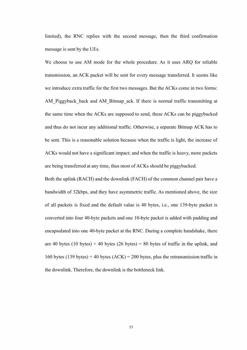
53

limited), the RNC replies with the second message, then the third confirmation

message is sent by the UEs.

We choose to use AM mode for the whole procedure. As it uses ARQ for reliable

transmission, an ACK packet will be sent for every message transferred. It seems like

we introduce extra traffic for the first two messages. But the ACKs come in two forms:

AM_Piggyback_back and AM_Bitmap_ack. If there is normal traffic transmitting at

the same time when the ACKs are supposed to send, these ACKs can be piggybacked

and thus do not incur any additional traffic. Otherwise, a separate Bitmap ACK has to

be sent. This is a reasonable solution because when the traffic is light, the increase of

ACKs would not have a significant impact; and when the traffic is heavy, more packets

are being transferred at any time, thus most of ACKs should be piggybacked.

Both the uplink (RACH) and the downlink (FACH) of the common channel pair have a

bandwidth of 32kbps, and they have asymmetric traffic. As mentioned above, the size

of all packets is fixed and the default value is 40 bytes, i.e., one 139-byte packet is

converted into four 40-byte packets and one 10-byte packet is added with padding and

encapsulated into one 40-byte packet at the RNC. During a complete handshake, there

are 40 bytes (10 bytes) + 40 bytes (26 bytes) = 80 bytes of traffic in the uplink, and

160 bytes (139 bytes) + 40 bytes (ACK) = 200 bytes, plus the retransmission traffic in

the downlink. Therefore, the downlink is the bottleneck link.

54

4.3.2 RRC Service and Channel Capacity

The two important criteria in the evaluation of RRC Service are loss rate and round-

trip time (RTT). Since AM mode is in use, all packets will be successfully delivered,

the loss rate is irrelevant, but the occasional losses contribute to RTT. In this specific

case, RTT is not merely the sum of multiple packet delays (i.e., three RRC signaling

messages). In addition to the end-to-end delay for individual packet, it also takes into

consideration the queueing delay, which is critical as this type of delay is the direct

indication of the packet scheduling mechanism in lower layers.

In order to find out how much of the channel capacity can be used for RRC Service,

our calculation is as follows:

Since the traffic generated for a complete handshake in the downlink is 200 bytes, the

downlink can support 32kbps/8*100sec = 400k bytes in 100secs, thus 400k bytes/200

bytes=2000 complete handshakes every 100 seconds.

We have 20 UEs in our simulation, provided the handshakes are equally distributed,

every UE is in charge of 2000/20 = 100 handshakes in 100 seconds, which

corresponds to an interval of 100/100 = 1/second. A uniform random variable

generator (with the min 90% and max 110%) is used for the intervals. Instead of being

a fixed number, the intervals lie within a range. Thus, the UEs are not synchronized and

do not send out requests at exactly the same time, but they still have roughly the same

intervals between requests, hence the total number of handshakes stays at the same

level. In this manner, extreme cases are avoided yet congestion situations can still be

55

tested.

We use different percent of the capacity to see the behavior of the transport channel.

Table 4.3 is the intervals and their range at different percent of channel capacity.

TableTableTableTable 4.34.34.34.3 IntervalIntervalIntervalIntervalCalculationsCalculationsCalculationsCalculations forforforfor OneOneOneOneGroupGroupGroupGroup

FigureFigureFigureFigure 4.24.24.24.25555 RRCRRCRRCRRC ServiceServiceServiceService atatatat DifferentDifferentDifferentDifferent%%%% ofofofof ChannelChannelChannelChannelCapacityCapacityCapacityCapacity

% bytes (KB) Interval (sec) Interval Range

10 40 10 [9, 11]

20 80 5 [4.5, 5.5]

30 120 3.3 [3, 3.6]

40 160 2.5 [2.25 2.75]

50 200 2 [1.8, 2.2]

60 240 1.67 [1.5, 1.84]

70 280 1.43 [1.29, 1.57]

80 320 1.25 [1.125, 1.375]

90 360 1.11 [1, 1.22]

100 400 1 [0.9, 1.1]

56

In Figure 4.25, when there is only pure RRC Service in the channel, the RTTs within

70% of channel capacity are of the same order, and then they start to grow

exponentially after that percentage. Considering the retransmission is also part of the

traffic, e.g. traffic at 100% is definitely over the full capacity, we define 70% as the

threshold, where the total traffic of the original transmission and the retransmission is

not over the full capacity.

FigureFigureFigureFigure 4.24.24.24.26666 RRCRRCRRCRRC ServiceServiceServiceService atatatat DifferentDifferentDifferentDifferent%%%% ofofofof ChannelChannelChannelChannelCapacityCapacityCapacityCapacity (10%-70%)(10%-70%)(10%-70%)(10%-70%)

In Figure 4.26, if we focus on the data from 10% to 70% of channel capacity when

there is only pure RRC Service in the channel, as the channel becomes more congested,

more packets start to drop, more retransmissions are required, and thus the RTTs

gradually increase. Nevertheless, the difference between RTTs at 10% and 70% is

smaller than 100ms.

57

4.3.3 RRC Service and DR Service

Now we add DR Service to the traffic.Normally, a plain-text DR message is about 500

bytes (or even bigger), with the help of XML compression techniques, this number can

be reduced to about 100 bytes. Here we use three different sizes of DR message and set

the interval so that the traffic from DR Service is 10% of the channel capacity, as

shown in Table 4.4.

10% of the channel capacity: 400K bytes*10%=40K bytes every 100 seconds

When DR messages are sent to customers, all end-devices in a neighborhood should

receive them. But the central DR system, which is located in the external network, does

not address distinct messages to individual users. Only one copy is sent to the BS and

the BS is in charge of broadcasting this message to all UEs within its coverage area.

Here we pick a random UE to receive DR messages from the central DR system, since

the common channel pair is shared by all UEs, when there are messages being

broadcast in the channel, every UE is guaranteed to receive one copy of its own.

TableTableTableTable 4.44.44.44.4 DifferentDifferentDifferentDifferent PacketPacketPacketPacket SizesSizesSizesSizes andandandandTheirTheirTheirTheir RespectiveRespectiveRespectiveRespective IntervalsIntervalsIntervalsIntervals

We use a UDP agent and CBR traffic generator to generate this type of traffic.

Packet Size # messages in 100 sec Interval (sec)

100 400 0.25

250 160 0.625

500 80 1.25

58

FigureFigureFigureFigure 4.24.24.24.27777 RRCRRCRRCRRC ServiceServiceServiceServicewithwithwithwith DRDRDRDR ServiceServiceServiceService atatatat 10%10%10%10% ofofofof ChannelChannelChannelChannelCapacityCapacityCapacityCapacity

In Figure 4.27, when a DR Service (10% of channel capacity) is added to the traffic,

between 80% and 100% of channel capacity, the growth in RTTs is much more

substantial compared to that with no DR Service.

FigureFigureFigureFigure 4.24.24.24.28888 RRCRRCRRCRRC ServiceServiceServiceServicewithwithwithwith orororor withoutwithoutwithoutwithout 10%10%10%10%DRDRDRDR ServiceServiceServiceService (10%-70%)(10%-70%)(10%-70%)(10%-70%)

In Figure 4.28, when there is a DR Service (10% of channel capacity) in addition to

RRC Service, the growth in RTTs between 10% and 70% is moderate. Compare the

59

traffic of additional 10% DR Service with that of pure RRC Service, we notice that

when more channel capacity is being used for RRC Service, the impact of DR Service

is more evident as the channel becomes more congested.

This type of DR Service is still heavy because DR Service is relatively delay-tolerant.

Customers only have to make their decisions in tens of minutes or hours, also the

wired link between DR server and RNC as well as the AM mode, makes sure that all

these DR messages are guaranteed to be successfully delivered to all customers. Hence,

low-frequency traffic should be considered.

We still use the three different sizes of message, but only send them once in 50 seconds.

FigureFigureFigureFigure 4.24.24.24.29999 RRCRRCRRCRRC ServiceServiceServiceServicewithwithwithwith Low-FrequencyLow-FrequencyLow-FrequencyLow-Frequency DRDRDRDR ServiceServiceServiceService (Interval:(Interval:(Interval:(Interval: 50505050 Seconds)Seconds)Seconds)Seconds)

In Figure 4.29, when a low-frequency DR Service, which broadcasts one DR message

every 50 seconds, is added to the traffic, these messages have less impact on RTTs

between 80% and 100% of channel capacity as these numbers are close to those with

no DR Service.

60

FigureFigureFigureFigure 4.4.4.4.30303030 RRCRRCRRCRRC ServiceServiceServiceServicewithwithwithwith orororor withoutwithoutwithoutwithoutLow-FrequencyLow-FrequencyLow-FrequencyLow-Frequency DRDRDRDR ServiceServiceServiceService (10%-70%)(10%-70%)(10%-70%)(10%-70%)

In Figure 4.30, when the additional DR Service is less frequent (one DR message every

50 seconds), and the RRC traffic occupies between 10% and 70% of channel capacity,

it practically does not affect RRC Service at all.

4.3.4 RRC Service and Grouping

Until now, we only consider the scenario that at the busiest hour, all RRC connection

procedures are equally distributed among all UEs. Here we divide the UEs into two

groups and three groups. Different groups have different number of call attempts in the

same amount of time, and thus have different intervals between calls, as shown in

Table 4.5 and Table 4.6. In the two-group scenario, there are 10 UEs in each group.

The first group is responsible for 500 out of 2000 complete handshakes whereas the

second one takes 1500 out of 2000.

61

TableTableTableTable 4.54.54.54.5 IntervalIntervalIntervalIntervalCalculationsCalculationsCalculationsCalculations forforforfor TwoTwoTwoTwoGroupsGroupsGroupsGroups

In the three-group scenario, there are 5 UEs in the first two groups and 10 in the last

group. And the handshakes are distributed as 500-1000-500 for groups, which

corresponds to 100-200-50 for each UE in the corresponding group.

% Bytes (KB) Interval (sec) Interval Range

10 5 20 [18,22]

15 6.67 [6,7.34]

20 10 10 [9,11]

30 3.33 [3,3.66]

30 15 6.67 [6,7.34]

45 2.22 [2,2.44]

40 20 5 [4.5,5.5]

60 1.67 [1.5,1.84]

50 25 4 [3.6,4.4]

75 1.33 [1.2,1.46]

60 30 3.33 [3,3.66]

90 1.11 [1,1.22]

70 35 2.85 [2.56,3.14]

105 0.95 [0.85,1.05]

62

TableTableTableTable 4.64.64.64.6 IntervalIntervalIntervalInterval CalculationsCalculationsCalculationsCalculations forforforfor ThreeThreeThreeThreeGroupsGroupsGroupsGroups

Based on the results above, 70% as the channel capacity threshold is confirmed. From

now on, we will only look at numbers between 10% and 70%.

% Bytes (KB) Interval (sec) Interval Range

10 10 10 [9,11]

20 5 [4.5,5.5]

5 20 [18,22]

20 20 5 [4.5,5.5]

40 2.5 [2.25,2.75]

10 10 [9,11]

30 30 3.33 [3,3.66]

60 1.67 [1.5,1.84]

15 6.67 [6,7.34]

40 40 2.5 [2.25,2.75]

80 1.25 [1.125,1.375]

20 5 [4.5,5.5]

50 50 2 [1.8,2.2]

100 1 [0.9,1.1]

25 4 [3.6,4.4]

60 60 1.67 [1.5,1.84]

120 0.83 [0.75.0.91]

30 3.33 [3,3.66]

70 70 1.43 [1.29,1.57]

140 0.714 [0.643,0.785]

35 2.86 [2.57,3.15]

63

FigureFigureFigureFigure 4.34.34.34.31111 RRCRRCRRCRRC ServiceServiceServiceService withwithwithwith orororor withoutwithoutwithoutwithoutLow-FrequencyLow-FrequencyLow-FrequencyLow-Frequency DRDRDRDR ServiceServiceServiceService (Two(Two(Two(Two

DifferentDifferentDifferentDifferentGroups)Groups)Groups)Groups)

FigureFigureFigureFigure 4.34.34.34.32222 RRCRRCRRCRRC ServiceServiceServiceService withwithwithwith orororor withoutwithoutwithoutwithoutLow-FrequencyLow-FrequencyLow-FrequencyLow-Frequency DRDRDRDR ServiceServiceServiceService (Three(Three(Three(Three

DifferentDifferentDifferentDifferentGGGGroups)roups)roups)roups)

In Figure 4.31 and Figure 4.32, when UEs are divided into different groups based on

their frequency of RRC connection attempts, the groups with more handshakes per UE

might have higher RTTs than those with fewer handshakes, but grouping does not

affect the average RTTs.

64

4.3.5 Confidence Intervals

We calculate the confidence intervals at 95% confidence level for this particular

scenario: no grouping is applied to all 20 UEs. The traffic from the original RRC

Service, along with that from a low-frequency DR Service, where the central DR

system broadcasts one 100-byte DR message every 50 seconds, co-exists in the shared

channel. This is the most plausible scenario from a planner’s point of view. In the same

neighborhood, the differences in the number of attempted connections from different

areas are not statistically significant enough. And under a normal circumstance, a low-

frequency DR Service is capable of delivering DR messages in a timely manner. We

start with numbers at 70% of channel capacity because if the difference at this point is

not statistically significant, it is neither at a lower percentage.

We compare one particular UE with the remaining 19 UEs. Out of these 20, there are

two cases where the ranges do not overlap at first. But when we prolong the simulation

time, they overlap after all.

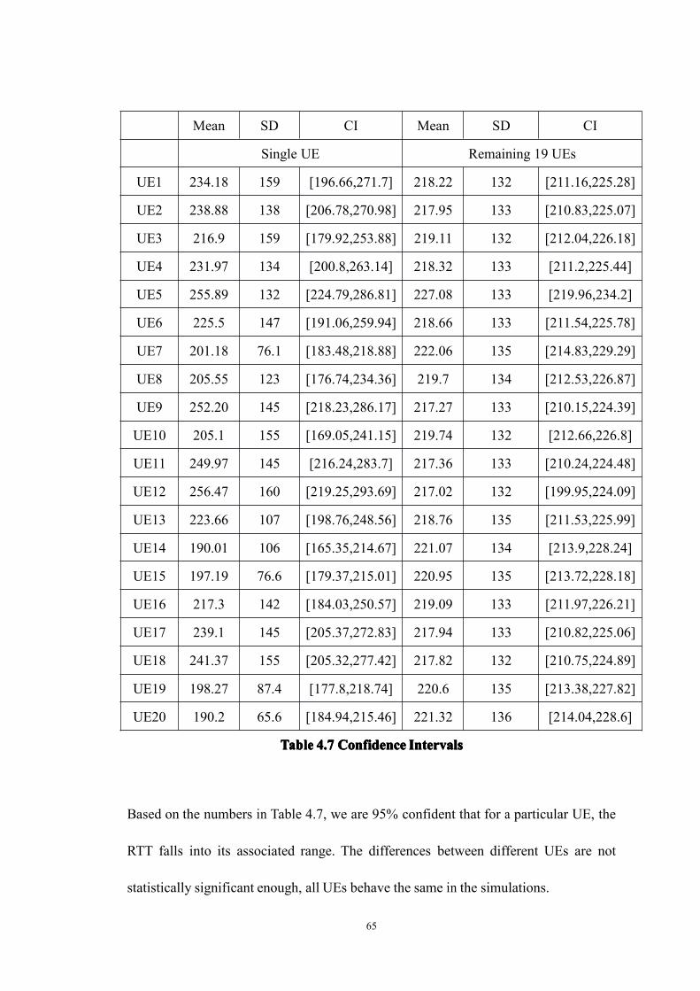
65

TableTableTableTable 4.74.74.74.7 ConfidenceConfidenceConfidenceConfidence IntervalsIntervalsIntervalsIntervals

Based on the numbers in Table 4.7, we are 95% confident that for a particular UE, the

RTT falls into its associated range. The differences between different UEs are not

statistically significant enough, all UEs behave the same in the simulations.

Mean SD CI Mean SD CI

Single UE Remaining 19 UEs

UE1 234.18 159 [196.66,271.7] 218.22 132 [211.16,225.28]

UE2 238.88 138 [206.78,270.98] 217.95 133 [210.83,225.07]

UE3 216.9 159 [179.92,253.88] 219.11 132 [212.04,226.18]

UE4 231.97 134 [200.8,263.14] 218.32 133 [211.2,225.44]

UE5 255.89 132 [224.79,286.81] 227.08 133 [219.96,234.2]

UE6 225.5 147 [191.06,259.94] 218.66 133 [211.54,225.78]

UE7 201.18 76.1 [183.48,218.88] 222.06 135 [214.83,229.29]

UE8 205.55 123 [176.74,234.36] 219.7 134 [212.53,226.87]

UE9 252.20 145 [218.23,286.17] 217.27 133 [210.15,224.39]

UE10 205.1 155 [169.05,241.15] 219.74 132 [212.66,226.8]

UE11 249.97 145 [216.24,283.7] 217.36 133 [210.24,224.48]

UE12 256.47 160 [219.25,293.69] 217.02 132 [199.95,224.09]

UE13 223.66 107 [198.76,248.56] 218.76 135 [211.53,225.99]

UE14 190.01 106 [165.35,214.67] 221.07 134 [213.9,228.24]

UE15 197.19 76.6 [179.37,215.01] 220.95 135 [213.72,228.18]

UE16 217.3 142 [184.03,250.57] 219.09 133 [211.97,226.21]

UE17 239.1 145 [205.37,272.83] 217.94 133 [210.82,225.06]

UE18 241.37 155 [205.32,277.42] 217.82 132 [210.75,224.89]

UE19 198.27 87.4 [177.8,218.74] 220.6 135 [213.38,227.82]

UE20 190.2 65.6 [184.94,215.46] 221.32 136 [214.04,228.6]

66

4.3.6 Conclusion

When DR Service is added to the existing RRC Service, it will always have an impact.

But if the traffic of RRC Service can stay within the threshold (70% of channel

capacity), no matter what is the size of DR messages or how all the handshakes are

distributed, the increase in RTTs can be kept minimal.

67

ChapterChapterChapterChapter 5555 XMLXMLXMLXMLCCCCompressionompressionompressionompressionTTTTechnologiesechnologiesechnologiesechnologies

The goal of this thesis is to explore the impact of DR Service if it is deployed over a

UMTS system, sharing resources with other traffic in the signaling channel. This DR

protocol is Extensible Markup Language (XML)-based. The central DR servers

convert the plain-text messages to XML format first before they are transferred to the

customers. The benefits of XML can be taken advantage of, and with the help of XML

compression technologies, we should be able to overcome the major obstacle of XML:

the resulting message size.

5.1 XML Overview

XML is a general-purpose markup language, which defines a set of annotations to

describe how text documents are formatted and can be used to facilitate the sharing of

structured data among heterogeneous information systems. It is a free open standard

recommended by the World Wide Web Consortium (W3C) and becomes very popular

through its standardization [45].

XML is designed to be simple and human legible (i.e. self-describing) [46]. For

example, a simple text format of a student record “100123456, Charlie M Brown, 123

Main Street, St Paul” can be presented like this.

68

<Student ID = “100123456”>

<FirstName>Charlie</FirstName>

<MInitial>M</MInitial>

<LastName>Brown</LastName>

<Address>123 Main Street, St Paul</Address>

</Student>

5.2 Compression Techniques

Because of its self-describing feature, XML introduces a significant amount of

redundant data, including white space, element and attribute names that add no useful

value. A raw XML document is expected to be larger than any other formats and can be

up to ten times as large as equivalent binary representation [47], thus severely affecting

the efficiency of communications since more network bandwidth and storage space are

required. Therefore, an effective compression technique is needed. This technique

should maintain the benefits that XML provides and improve the usage of these

resources at the same time.

As far as we are concerned, the most important evaluation criterion should be the

complexity of output documents. The end-user devices are equipped with very limited

computing resources, the messages they receive must be easy to process. As for the

characteristics of output documents, messages for both price events and emergency

events are usually small (several hundred bytes), less frequent (at most a few every

69

hour) and relatively delay-tolerant (responses can be made within tens of minutes or

even longer), therefore, the compression time, which is in the order of seconds, is less

critical. Meanwhile, even though the storage spaces in these devices are finite, due to

the time-sensitive nature of these messages, they will only be processed once at most,

so the compression ratio, which restricts the sizes of output documents, is not that

important. However, because the traffic that goes through the whole network matters, it

is taken into consideration as the second important criterion.

Since XML documents are represented as text files, a general-purpose compressor is

always an obvious choice. Currently, many open-source (e.g. gzip [48]) and

commercial (e.g. WinZip [49]) implementations are already available. They provide a

decent compression ratio (40%-50%) of the original files; they require no knowledge

of the document structure because they are generic; they are universal that they are

built into many applications as one of the standard features. While they are

straightforward and easy to manage, the disadvantages they possess happen to conflict

with the requirements of our task. These techniques tend to require significant

processor capabilities and memory spaces, and they only work best with large files as

the performance degrades when file size decreases.

XML imposes basic syntax constraints on documents itself. An XML schema [50] [51],

which provides other validity criteria, defines constraints on the structure and content

of a certain document type as well. The schema-aware XML compressors virtually all

have used gzip or equivalent as the core compression technique. With the help of other

pre-processing routines, this kind of hybrid techniques can perform significantly better

70

than using gzip alone. XMill (AT&T) [52] claims that it can achieve twice the

compression ratio of gzip in roughly the same amount of time. Technically, it does not

rely on information from a Document Type Definition (DTD) or an XML schema

Definition (XSD) file, yet it exploits hints about such schemas in order to further

improve the compression ratio. As shown in Figure 5.1, the pre-processing routine

separates the structure (tags and attributes) from the data (text content and attribute

values) and these two are compressed separately. After being passed through the SAX

parser, the data from XML documents are grouped into different containers based on

the different expressions that they match. This can be done by either following the

default setup or explicitly specifying these expressions. These unique containers are

then passed to gzip and specialized semantic compressors are applied to them.

Different semantic compressors can be created for basic, combined or user-defined data

types. Hence, a higher compression ratio is not surprising. Nevertheless, because

human intervention is required to achieve the best result and the pre-processing of

compressed documents actually hinders compressors other than gzip, unless the

network bandwidth is extremely scarce and the message size is considerably large,

XMill would not be considered as the best choice for our task.

71

FigureFigureFigureFigure 5.15.15.15.1 Pre-ProcessingPre-ProcessingPre-ProcessingPre-ProcessingCompressorCompressorCompressorCompressor

XComp [53] is another compressor that shares the same principle with XMill.

Additionally, every distinct attribute is assigned a positive integer as their IDs and a

sequence of these integers is used to keep track of the data items’ positions.

Furthermore, the boundary size for XComp is 4K bytes whereas the one for XMill is

20K bytes. Therefore, XComp not only outperforms XMill in terms of compression

ratio, but is also a better choice for smaller messages. However, the same problem

exists for XComp. When the size of the input document is lower than this boundary,

XComp does not exhibit any overwhelming advantage.

XGrind [54] and Xpress [55] also compress XML documents by separating the

structure from the data, but the compressors maintain the structure of the input

72

documents the whole time, thus make the compressed documents queryable, i.e. the

output files can be directly queried before being fully decompressed. In addition,

XGrind keeps DTD files as well. This is very important for resource-limited wireless

devices as they can reuse them for the following compression/decompression. And

even resources might be adequate, querying on compressed documents reduces

network bandwidth usage and query response time.

Because of the textual heritage and many rules it imposes, XML is and will always be

verbose. Data compression is one way to solve this problem. Other than the techniques

mentioned above, one can always design a specific compressor for a specific task. This

will guarantee the best performance as all messages are in the same format and the

format is already known in advance. Nevertheless, this approach does limit the

flexibility of the application. When some modifications are made, this custom-made

compressor becomes an obstacle instead. Another solution is Binary XML [56] [57]

[58], which encodes XML documents in a binary data format rather than plain text.

Even though no format has been accepted as the de facto standard, using a Binary

XML format generally decreases the file size, reduces the verbosity of XML

documents and lowers the cost for required processing. Therefore it would greatly

benefit wireless devices with limited capabilities. The comparison of XML

compression technologies is presented in Table 5.1.

73

TableTableTableTable 5.15.15.15.1 ComparisonComparisonComparisonComparison ofofofof XMLXMLXMLXML CompressionCompressionCompressionCompressionTechnologiesTechnologiesTechnologiesTechnologies

Because of its simplicity, XML can be exploited to benefit resource-limited wireless

devices as only primitive computing is required. With its growing popularity, it is

natural to expect that not only DR messages, but also the data from other applications

will be represented in this format. Since XML documents are usually larger in size than

any other formats that contain the same amount of data, this size problem substantially

increases the costs of processing, storing and exchanging the data, and becomes a huge

hindrance for any bandwidth-related applications.

DR Service has very limited impact on RRC Service when its frequency is low,

regardless of the size of DR messages. But the difference does exist as shown in Figure

4.29, larger DR messages increase the RTTs more than smaller DR messages do,

especially between 80% and 100% of channel capacity. Because the size of all lower

layer packets is fixed and the default value is 40 bytes, large messages from upper

Complexity of

output

documents

Utilization of

XML schema

Pre-processing Compression

ratio

General

compressor (gzip)

High No No Good

XMill High No Yes Good

XComp High No Yes Good

XGrind/XPress Low Yes/No Yes Good

Custom-made

compressor

Low Yes N/A Great

Binary XML Low N/A N/A Great

74

layers are encapsulated into multiple small packets. Thus, a large message creates a

more "bursty" traffic, i.e., when one 500-byte message arrives at the RNC, it becomes

thirteen packets. This type of traffic has a more significant impact during the busiest

hour.

gzip provides a 40%-50% compression ratio of XML documents, and XMill and other

technologies claim they can achieve at least twice the compression ratio of gzip's.

Therefore, we expect the size of a compressed 500-byte DR message to be between

100 bytes and 250 bytes, and this also explains why we choose these three sizes for our

simulations.

The difference between a 500-byte message and a 100-byte message is 400 bytes, it is

equal to 10% of channel capacity of the common channel (400bytes/32kbps/8=10%).

Even though it is highly unlikely that we will schedule a DR message every second, but

the wireless link quality might be very poor that we need more retransmissions under

some circumstances. This difference cannot be overlooked.

The XML compression technologies we have reviewed above provide a means to

reduce the size of XML documents to a reasonable level. Therefore, in our task, the

XML-formatted DR messages are easy for end-devices to handle, and they have

minimal impact on RRC Service as well as the network efficiency.

75

ChapterChapterChapterChapter 6666 ConclusionsConclusionsConclusionsConclusions

In this thesis, the additional MAC and PHY layer support, which is provided by the

EURANE extension in addition to NS-2, enable us to test channel access mechanisms

other than simple routing and forwarding protocols.

With the architecture of the UMTS system in mind, we are able to construct topologies

for the UMTS network and focus on the wireless link between the UTRAN and UEs.

Demand Response mechanisms provide power grid operators a method to dynamically

manage electricity demand from customers and maintain a stable power supply level.

By following the recommended instructions from the central DR system, customers

can also reduce their overall electricity bills. This type of mechanisms can be

implemented over various platforms, with different limits applied to them. In this

thesis, the UMTS (3G) network is chosen as the carrier. We can either allocate unique

resources for DR Service or integrate it onto a shared channel with other existing

services. In the latter's case, the impact of DR Service has to be evaluated.

We fully utilize the different RLC modes, transport layer agents to test the transport

channels in ideal PHY environment. They are compared in terms of loss rate and

average delay. Out of these six combinations: TCP-RACH/FACH, UDP-RACH/FACH,

TCP-DCH/DCH, UDP-DCH/DCH, TCP-DCH/HS-DSCH, UDP-DCH/HS-DSCH,

the UDP cases outperform the TCP cases in general. And UDP-RACH/FACH, UDP-

DCH/DCH and UDP-DCH/HS-DSCH are all capable of delivering DR Service.

76

The simulations are not limited to ideal PHY environment. We follow the instructions

to generate "input tracefiles" as the PHY layer support to see how HS-DSCH behaves

in more realistic environments. The results show that even without any retransmission

mechanism, this channel can provide decent performance in small cell and low

transmit power (Indoor Office and Pedestrian) environment, which are the locations of

our potential customers.

Our ultimate goal is to integrate DR Service with some other services within the

UMTS framework. DR Service is packet-oriented, thus it does not first establish a

connection, whereas in the UMTS system, the RRC connection establishment

procedures are required for UEs before they can make use of the radio resources. If

these two types of service can co-exist in a shared channel, the bandwidth of this

channel can be utilized to the maximum. We need to explore if the additional DR

Service affects the original RRC Service, and it turns out a moderate level of DR

Service does not have a significant impact, even at the busiest hour.

The above is what we have covered in this thesis. It provides answers to many

questions.

� Incorporating DR Service to the UMTS system is feasible.

� In ideal PHY environment, transport channel pairs RACH/FACH, DCH/DCH and

DCH/HS-DSCH are all suitable for DR Service if its traffic is in a separate

channel.

� Without retransmission mechanism, HS-DSCH works well in small cell and low

77

transmit power (Indoor Office and Pedestrian) environments.

� When DR Service and RRC Service co-exist in a shared channel, if the frequency

of DR Service is low, it will only have a very limited impact.

� For motivation purposes, DR Service is used here as an example. A simple service

like this will not generate a significant amount of traffic. Other services including

weather update, stock and traffic information can be offered through the UMTS

system the same way. They only require one-way communication (broadcast) and

generate the same type of traffic as DR Service. Our results show that as long as

the aggregate traffic by all these additional services does not exceed 10% of

channel capacity, they will not significantly affect the efficiency of RRC Service.

� Compression technologies can help the XML-based DR system to reduce the size

of DR messages, and to minimize their impact on RRC Service and network

efficiency.

However, some issues are left for future work.

� The NS-2 offers standard error models for the common channel pair

RACH/FACH, but the limitations are obvious. It would be nice to have diverse

ways to add impact to the PHY layer: multipath fading, co-channel interference,

etc.

�� Currently, DR Service uses a one-way communication system, where end-devices

only receive DR messages. In the near future, customers may have the ability to

78

give feedback to the central DR system, which can help power grid operators to

make their decisions and plans.

�� The comparison among different transport channel pairs has some surprising

results when TCP is used as a transport protocol. HS-DSCH offers higher peak

data rates and throughput than any other downlink transport channels, yet it has a

lower average throughput than DCH. This is not unusual as there is some research

about this topic, however, a definite answer has not yet been given.

79

ReferencesReferencesReferencesReferences

[1] OECD Publishing, "The Power to Choose: Demand Response in Liberalised

Electricity Markets", Paris, France, International Energy Agency, ISBN: 978-

9264105034, 2003.

[2] A. Chen, "Multi-Building Internet Demand Response Control System: the First

Successful Test", [Online document] Feb. 2004. Available at HTTP:

http://www.lbl.gov/Science-Articles/Archive/EETD-demand-response.html

[3] W. Badgley, "Electricity and Its Source", Whitefish, Montana, Kessinger

Publishing, ISBN: 978-0548933084, 2008.

[4] T. Elliott, K. Chen and R. Swanekamp, "Standard Handbook of Powerplant

Engineering", New York, New York, McGraw-Hill Professional, ISBN: 978-

0070194359, 1997.

[5] A. Thumann and S. Dunning, "Plant Engineers and Managers Guide to Energy

Conservation", London, England, CRC Press, ISBN: 978-1420052466, 2008.

[6] L. Dyckman and J. Jones, "Renewable Energy: Wind Power's Contribution to

Electric Power Generation and Impact on Farms and Rural Communities", Darby,

Pennsylvania, Diane Publishing Co, ISBN: 978-0756745783, 2004.

[7] H. Termuehlen, "100 Years of Power Plant Development", New York, New York,

Amer Society of Mechanical Engineers, ISBN: 978-0791801598, 2001.

http://www.lbl.gov/Science-Articles/Archive/EETD-demand-response.html

80

[8] M. El-Wakil, "Power Plant Technology", New York, New York, McGraw-Hill

Professional, ISBN: 978-0070662742, 1985.

[9] H. Herzog and J. Katzer, "The Future of Coal in a Greenhouse Gas Constrained

World", Presented at the 8th International Conference on Greenhouse Gas Control

Technologies, Trondheim, Norway, 2006.

[10] CBC News Online, "Indepth: Power Outage", [Online document] Aug. 2003.

Available at HTTP: http://www.cbc.ca/news/background/poweroutage/

[11] J. Barron, "The Blackout of 2003: The Overview; Power Surge Blacks Out

Northeast, Hitting Cities in 8 States and Canada; Midday Shutdowns Disrupt Millions",

NYTimes Journal Archive, Aug. 2003.

[12] California Energy Commission Home Page, http://www.energy.ca.gov/

[13] Programmable Communicating Thermostat (PCT),

http://sharepoint.californiademandresponse.org/pct/

[14] E. Gunther, "Reference Design for Programmable Communicating Thermostats

Compliant with Title 24-2008", [Online document] Oct. 2007. Available at HTTP:

http://sharepoint.californiademandresponse.org/pct/Shared%20Documents/Reference

DesignTitle24PCT-%20rev17b.doc

[15] GridWise at PNNL, http://gridwise.pnl.gov/

[16] BPA-Energy Efficiency|Energy Web,

http://www.bpa.gov/Energy/N/tech/energyweb/

[17] California ISO, http://www.caiso.com/

http://www.cbc.ca/news/background/poweroutage/

http://www.energy.ca.gov/

http://sharepoint.californiademandresponse.org/pct/

http://sharepoint.californiademandresponse.org/pct/Shared%20Documents/ReferenceDesignTitle24PCT-%20rev17b.doc

http://sharepoint.californiademandresponse.org/pct/Shared%20Documents/ReferenceDesignTitle24PCT-%20rev17b.doc

http://gridwise.pnl.gov/

http://www.bpa.gov/Energy/N/tech/energyweb/

http://www.caiso.com/

81

[18] CEC's Public Interest Energy Research (PIER) Program,

http://www.energy.ca.gov/pier/

[19] Independent Electricity System Operator (IESO), http://www.ieso.ca/

[20] OPA-Ontario Power Authority, http://www.powerauthority.on.ca/

[21] Toronto Hydro Corporation, http://www.torontohydro.com/

[22] S. Jewell et al, "Cable TV Technology for Local Access", BT Technology Journal,

vol. 16, no. 4, pp. 80-91.

[23] L. Harte, "Introduction to Mobile Telephone Systems, 2nd edition, 1G, 2G, 2.5G,

and 3G Technologies and Services", Fuquay Varina, North Carolina, Althos, Inc, ISBN:

978-1932813937, 2006.

[24] V. Chitre and J. Daigle, "IP-Based Services over GPRS", ACM SIGMETRICS

Performance Evaluation Review, vol. 28, no. 3, pp. 39-47.

[25] A. Mehrotra, "GSM System Engineering, 1st edition", Norwood, Massachusetts,

Artech House, Inc, ISBN: 978-0890068601, 1997.

[26] S. Redl, M. Weber and M. Oliphant, "An Introduction to GSM, 1st edition",

Norwood, Massachusetts, Artech House, Inc, ISBN: 978-0890067857, 1995.

[27] H. Wesolowski and K. Wesolowski, "Mobile Communication Systems", New

York, New York, John Wiley & Sons, Inc, ISBN: 978-0471498377, 2002.

[28] C. Smith, "3G Wireless Networks", New York, New York, McGraw-Hill

Professional, ISBN: 978-0072263442, 2001.

[29] ETSI, http://www.etsi.org/

http://www.energy.ca.gov/pier/

http://www.ieso.ca/

http://www.powerauthority.on.ca/

http://www.torontohydro.com/

http://www.etsi.org/

82

[30] V. Dubendorf, "Wireless Data Technologies Reference Handbook", New York,

New York, John Wiley & Sons, Inc, ISBN: 978-0470849491, 2003.

[31] J. Korhonen, "Introduction to 3G Mobile Communication, 2nd edition", Norwood,

Massachusetts, Artech House, Inc, ISBN: 978-1580535076, 2003.

[32] J. Castro, "The UMTS Network and Radio Access Technology: Air-Interface

Techniques for Future Mobile Systems", New York, New York, John Wiley & Sons,

Inc, ISBN: 978-0471813750, 2001.

[33] Twente Institute for Wireless and Mobile Communications (WMC), "End-to-end

Network Model for Enhanced UMTS", [Online document] Oct. 2003. Available at

HTTP: http://eurane.ti-wmc.nl/eurane/D32v2Seacorn.pdf.gz

[34] 3rd Generation Partnership Project (3GPP), "3GPP TS 25.211, Physical Channels

and mapping of Transport Channels onto Physical Channels (FDD)", 3GPP

Specification Archive, Sept. 2002.

[35] ETSI MCC Department, "Overview of 3GPP Release 99, Summary of all Release

99 Features", ETSI Mobile Competence Centre, May. 2004.

[36] 3rd Generation Partnership Project (3GPP), "3GPP TR 25.855, High Speed

Downlink Packet Access (HSDPA); Overall UTRAN Description", 3GPP

Specification Archive, Oct. 2001.

[37] The Network Simulator-NS-2, http://www.isi.edu/nsnam/ns/

[38] EURANE Website, http://eurane.ti-wmc.nl/eurane/

[39] SEACORN, http://seacorn.ptinovacao.pt/

http://eurane.ti-wmc.nl/eurane/D32v2Seacorn.pdf.gz

http://www.isi.edu/nsnam/ns/

http://eurane.ti-wmc.nl/eurane/

http://seacorn.ptinovacao.pt/

83

[40] Twente Institute for Wireless and Mobile Communications (WMC), "Enhanced

UMTS Radio Access Network Extensions for NS-2 (EURANE) User Guide", [Online

document] Sept. 2005. Available at HTTP: http://eurane.ti-

wmc.nl/eurane/eurane_user_guide_1_6.pdf

[41] S. Nadas et al, "Providing Congestion Control in the Iub Transport Network for

HSDPA", Global Telecommunications Conference GLOBECOM ‘07, Budapest,

Hungary, 2007, pp. 5293-5297.

[42] Canadian Evaluation Group (CEG), "ITU ITU-R M.1225, Guidelines for

Evaluations of Radio Transmission Technologies for IMT-2000", International

Telecommunication Union (ITU) Radiocommunication Sector, Jan. 1997.

[43] 3rd Generation Partnership Project (3GPP), "3GPP TS 25.331, Radio Resource

Control (RRC); Protocol Specification", 3GPP Specification Archive, Dec. 2001.

[44] QUALCOMM Europe, "Updating Encryption Keys for MBMS", Presented at

3GPP TSG SA WG3 Security--MBMS ad-hoc, Antwerp, Belgium, 2003.

[45] Extensible Markup Language (XML), http://www.w3.org/XML/

[46] S. Hollenbeck, M. Rose and L. Masinter, "RFC3470: Guidelines for the Use of

Extensible Markup Language (XML) within IETF Protocols", Internet Society (ISOC),

Jan. 2003.

[47] D. Megginson, "XML Performance and Size", [Online Document] Mar. 2005.

Available at HTTP: http://www.informit.com/articles/article.aspx?p=367637

[48] The gzip home page, http://www.gzip.org

http://eurane.ti-wmc.nl/eurane/eurane_user_guide_1_6.pdf

http://eurane.ti-wmc.nl/eurane/eurane_user_guide_1_6.pdf

http://www.w3.org/XML/

http://www.informit.com/articles/article.aspx?p=367637

http://www.gzip.org

84

[49] WinZip-The Zip File Utility for Windows-Zip/Unzip, Encrypt/Decrypt,

http://www.winzip.com

[50] C. Campbell, A. Eisenberg and J. Melton, "XML Schema", ACM SIGMOD

Record, vol. 32, no. 2, pp. 96-101.

[51] G. Bex, F. Neven and J. Bussche, "DTDs Versus XML Schema: A Practical Study",

Proceedings of the 7th International Workshop on the Web and Databases: Colocated

with ACM SIGMOD/PODS 2004, Paris, France, 2004, pp. 79-84.

[52] H. Liefke and D. Suciu, "XMill: An Efficient Compressor for XML Data",

Proceedings of the 2000 ACM SIGMOD International Conference on Management of

Data, Dallas, Texas, 2000, pp. 153-164.

[53] W. Li, "XComp: An XML Compression Tool", Master's Thesis, University of

Waterloo, Waterloo, Ontario, 2003.

[54] P. Tolani and J. Harista, "XGrind: A Query-Friendly XML Compressor",

Proceedings of the 18th International Conference on Data Engineering, San Jose,

California, 2002, pp. 225-234.

[55] J. Min, M. Park and C. Chung, "Xpress: A Queryable Compression for XML

Data", Proceedings of the 2003 ACM SIGMOD International Conference on

Management of Data, San Diego, California, 2003, pp. 122-133.

[56] C. Augeri et al, "An Analysis of XML Binary Formats and Compression",

Proceedings of Experimental Computer Science on Experimental Computer Science,

San Diego, California, 2007, pp. 6-6

http://www.winzip.com

85

[57] C. Augeri et al, "An Analysis of XML Compression Efficiency", Proceedings of

the 2007 Workshop on Experimental Computer Science, San Diego, California, 2007,

Article No.7.

[58] K. Chiu et al, "A Binary XML for Scientific Applications", Proceedings of the 1st

International Conference on E-Science and Grid Computing, Melbourne, Australia,

2005, pp. 336-343.