Phase I Report of the American Academy of Actuaries' C-3 Subgroupof the Life Risk Based Capital Task Force to the National Association of

Insurance Commissioners' Risk Based Capital Work GroupOctober 1999 - Atlanta, GA

The American Academy of Actuaries is the public policy organization for actuariespracticing in all specialties within the United States. A major purpose of the Academy isto act as the public information organization for the profession. The Academy is non-partisan and assists the public policy process through the presentation of clear andobjective actuarial analysis. The Academy regularly prepares testimony for Congress,provides information to federal elected officials, comments on proposed federalregulations, and works closely with state officials on issues related to insurance. TheAcademy also develops and upholds actuarial standards of conduct, qualification andpractice and the Code of Professional Conduct for all actuaries practicing in the UnitedStates.

This report was prepared by the American Academy of Actuaries Life Risk-based CapitalTask Force.

C-3 Subgroup of the Life Risk-Based Capital Task Force

Robert A. Brown, F.S.A., M.A.A.A., Chair

Errol Cramer, F.S.A., M.A.A.A. Joseph L. Dunn, F.S.A., M.A.A.ACraig Fowler, F.S.A. Glenn Keller, F.S.A., M.A.A.A.Alastair Longley-Cook, F.S.A., M.A.A.A. James F. Reiskytl, F.S.A., M.A.A.A.Linn K. Richardson, F.S.A.,M.A.A.A. Mark C. Rowley, F.S.A., M.A.A.A.David K. Sandberg, F.S.A., M.A.A.A. Stephen A.J. Sedlak, F.S.A., M.A.A.A.James A. Tolliver, F.S.A., M.A.A.A. Bill Wilton, F.S.A., M.A.A.A.Michael L. Zurcher, F.S.A., M.A.A.A.

2

Table of Contents

I. Acknowledgements - Page 3

II. Executive Summary - Pages 4-6

III. Appendix I - Scenario Testing Methodology - Pages 7-9

IV. Appendix II - Frequently Asked Questions - Page 10-11

V. Appendix III - Technical Aspects of the Scenario Generator and the ScenarioSelection Process - Pages 12-15

VI. Appendix III, Section A - Page 16

VII. Appendix III, Section B - Page 17-19

VIII. Appendix III, Section C - Page 20

IX. Appendix IV, C-3 Pilot Testing: Results from the "50" Scenario Subset - Pages21-23

X. Draft Instructions

3

Acknowledgements

In addition to the members of the Academy's C-3 Subgroup, contributing to the reportwere Ron Rubnich, Steve Ekblad, and Lloyd Spencer. Their efforts are greatlyappreciated. Also, thanks is due to the full Life Risk Based Capital Task Force at theAcademy for their efforts.

4

Executive Summary

Background

Several years ago, the NAIC Life Risk Based Capital Working Group asked the AAALife Risk Based Capital Task Force to take a fresh look at the C-3 component of the RBCformula to see if a practical method could be found to reflect the degree of asset/liabilitymismatch risk of a particular company.

We reviewed the request and we agree that more sensitivity to the specifics of productdesign and funding strategy is appropriate to advance the goal of differentiating weaklycapitalized companies from the rest. We have determined that, due to the widespread useof increasingly well disciplined scenario testing for Asset Adequacy Analysis, afoundation now exists for such an improvement. For this purpose, we have defined C-3risk to include Asset/Liability risk in general, not just interest rate risk. However, thisrecommendation does not address refining the measurement for other than interest raterisk, since doing so would require introduction of a model of stock market performance.Addressing these products is one of the “next steps” suggested.

Our recommendation is to change the method of developing the C-3 component of RBC,effective 12/31/2000, building on the work of the asset adequacy modeling, but usinginterest scenarios designed to help approximate the 95th percentile C-3 risk.

Recommendation

The revised C-3 component is to be calculated as the sum of three amounts, but subject toa minimum and maximum. The calculation is:

a) For Annuities or Single Premium Life Insurance products, whether written directly orassumed through reinsurance, that the company tests for Asset Adequacy Analysis usingcash flow testing, the C-3 requirement is calculated based on the same cash flow models,assets, and assumptions used and same “as-of” date as for Asset Adequacy, but with adifferent set of interest scenarios, and a different measurement of results. A weightedaverage of a subset of the scenario specific results is used to determine the C-3requirement. If the “as-of” date of this testing is not 12/31, the ratio of the C-3requirement to reserves on the “as-of” date is applied to the year end reserves, similarlygrouped, to determine the year-end C-3 requirement for this category. With respect toreinsured ceded or assumed business, Asset Adequacy Analyses should be based on therisk actually retained or assumed, and reflect expected experience rating and otheradjustments based on the scenarios tested. Equity indexed products are to use the existingfactors, not the results of scenario testing.

5

b) For all other products (either non-cash-flow-tested or those outside the product scopedefined above) the C-3 requirements are calculated using current existing factors andinstructions.

c) For callable assets (including IOs and similar investments) supporting untestedproducts and surplus the C-3 requirement is 50% of the excess, if any, of statementvalue above current call price (calculated on an asset by asset basis).

The total C-3 component is the sum of a, b, and c, but not less than half nor more thandouble the C-3 component based on current factors and instructions.

• For this recommendation, “annuities” means products with the characteristics ofdeferred and immediate annuities, structured settlements, guaranteed separateaccounts, and GICs (including synthetic GICs, and funding agreements). If cash flowtesting of debt incurred for funding an investment account is required by the insurer’sstate of domicile for asset adequacy analysis, it is included. Equity based variableproducts are not to be included, but products that guarantee a bond index and variableannuities sold as fixed are, if they are cash flow tested.

• The company may use either a standard 50 scenario set of interest rates or analternative, but more conservative, 12 scenario set (for part a, above). It may use thesmaller set for some products and the larger one for others, but aggregation will thenonly be available among products using the same scenario sets. Details of thescenario testing methodology are contained in Appendix I.

• In order to allow time for the additional work effort needed for the new approachwhile not delaying filing dates, we recommend that an estimated value be permittedfor the year end statement. For the RBC diskette filing, these C-3 results must bedetermined by scenario. If the actual RBC value exceeds that estimated earlier in theblanks filing by more than 5%, or if the actual value triggers regulatory action, arevised filing of that statement page with the NAIC and the state of domicile isrequired by June 15, otherwise it is permitted but not required.

• The diskette submission will be accompanied by a statement from the AppointedActuary certifying that in his or her opinion the assumptions used for thesecalculations are not unreasonable for the products, scenarios, and regulatory purposebeing tested.

• The scenario testing used for this purpose will use the same assumptions as to cashflows, assets associated with tested liabilities, future investment strategy, rate spreads,credit losses, “as-of” date and treatment of negative cash flows as were used for cashflow testing (except that if negative cash flow is modeled by borrowing, the actuaryneeds to make sure that the amount and cost of borrowing are reasonable for thatparticular scenario of the C-3 testing) The other differences are the interest scenariosthemselves and how the results are used.

6

• The actuary must also assure that the cash flow testing used for the 50 or 12 scenariosdoes not double count cash flow offsets to the interest rate risks. That is that thecalculations do not reduce C-3 and another RBC component for the same margins.For example, certain reserve margins on some guaranteed separate account productsserve an AVR role and are credited against the C-1 requirement. To that degree,these margins should be removed from the reserve used for C-3 testing.

• Sensitivity testing of key assumptions such as lapses is required.

Next Steps

Although this report is our final recommendation for “Phase I” of our project, at least twoareas of unfinished business remain:

a) Review of the Outcomes of this Revised Approach

The C-3 result under this recommendation is limited to between half and twice thecurrent factors. This was done in part to limit the severity of the impact of the changeuntil the results of this method could be evaluated. Substantial testing of this approachwas done for a variety of products and portfolios, but, unlike most of the prior changes toRisk Based Capital, the industry-wide impact of this change couldn’t be measured inadvance. If the industry-wide results (both statistical and anecdotal) show a distributionof outcomes that seems believable, it may be desirable to widen this range. If the resultsare puzzling, then we would want to pursue further research to evaluate the outliers.

b) Expansion to Equity Indexed and Variable products

Aside from a guaranteed fixed option within a variable product, these two product groupsrequire modeling beyond the scope of our “Phase I” project, since they also involvebehavior of indices or of funds. Expanding the C3 work to encompass these products in amore refined manner than today is appropriate in the future.

7

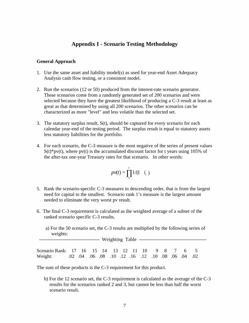
Appendix I - Scenario Testing Methodology

General Approach

1. Use the same asset and liability model(s) as used for year-end Asset AdequacyAnalysis cash flow testing, or a consistent model.

2. Run the scenarios (12 or 50) produced from the interest-rate scenario generator.These scenarios come from a randomly generated set of 200 scenarios and wereselected because they have the greatest likelihood of producing a C-3 result at least asgreat as that determined by using all 200 scenarios. The other scenarios can becharacterized as more "level" and less volatile than the selected set.

3. The statutory surplus result, S(t), should be captured for every scenario for eachcalendar year-end of the testing period. The surplus result is equal to statutory assetsless statutory liabilities for the portfolio.

4. For each scenario, the C-3 measure is the most negative of the series of present valuesS(t)*pv(t), where pv(t) is the accumulated discount factor for t years using 105% ofthe after-tax one-year Treasury rates for that scenario. In other words:

∏ +=t

titpv1

1/(1)( )

5. Rank the scenario-specific C-3 measures in descending order, that is from the largestneed for capital to the smallest. Scenario rank 1’s measure is the largest amountneeded to eliminate the very worst pv result.

6. The final C-3 requirement is calculated as the weighted average of a subset of theranked scenario specific C-3 results.

a) For the 50 scenario set, the C-3 results are multiplied by the following series ofweights:

------------------------------------- Weighting Table -----------------------------------------

Scenario Rank: 17 16 15 14 13 12 11 10 9 8 7 6 5Weight: .02 .04 .06 .08 .10 .12 .16 .12 .10 .08 .06 .04 .02

The sum of these products is the C-3 requirement for this product.

b) For the 12 scenario set, the C-3 requirement is calculated as the average of the C-3results for the scenarios ranked 2 and 3, but cannot be less than half the worstscenario result.

8

7. If multiple asset/liability portfolios are tested and aggregated, the aggregate C-3requirement can be derived by first summing the S(t)'s from all the portfolios (byscenario) and then following steps 4 through 6. An alternative method is to calculatethe C-3 result by scenario for each product, sum them by scenario, rank-order them,and then apply the above weights. If some products are tested with 12 scenarios andsome with 50, aggregation can only be done within like scenario sets.

Single Scenario C-3 Measurement Considerations

1. GENERAL METHOD - this approach incorporates interim values, consistent withapproach used for bond, mortgage and mortality RBC factor quantification. Theapproach establishes the risk measure in terms of an absolute level of risk (e.g.,solvency) rather than volatility around an expected level of risk. It also recognizesreserve margins, to the degree that such margins haven’t been recognized for orused to offset other RBC requirements.

2. INITIAL ASSETS = RESERVES - consistent with Appointed Actuary practice, theasset adequacy cash flow models are run with initial assets equal to reserves; thatis, no surplus assets are used.

3. AVR – Although AVR and related assets are usually included in initial assets forAsset Adequacy cash flow testing, they should not be included in the initial assetsused in the C-3 modeling. These assets are available for future credit lossdeviations over and above expected credit losses. These deviations are covered byC-1 RBC requirements. Similarly, future AVR contributions should not bemodeled. However, expected credit losses, which are not covered by C-1, shouldbe modeled.

4. IMR –The IMR reserve, assets, and run-off schedule associated with a category (a)product should be included in that product’s cash flow modeling for determinationof RBC. If a callable asset is called below carrying value, the IMR modelingshould reflect the impact of that loss.

5. INTERIM MEASURE - retained statutory surplus S(t) (i.e., statutory assets lessstatutory liabilities) is used as the year-to-year interim measure.

6. TESTING HORIZONS - surplus adequacy should be tested over a period thatextends to a point at which contributions to surplus on a closed block areimmaterial in relationship to the analysis. If some products are being cash flowtested for Asset Adequacy Analysis over a longer period than the 30 yearsgenerated by the interest rate scenario generator, the scenario rates should be heldconstant at the year 30 level for all future years. A consistent testing horizon isrequired for all lines tested if the C-3 results from different lines of business are tobe aggregated.

9

7. TAX TREATMENT - the tax treatment should be the same as that used forAssetAdequacy Analysis. Disclosure of tax assumptions may be required.

8. REINVESTMENT STRATEGY - the reinvestment strategy should be the same asthat used for Asset Adequacy Analysis cash flow testing.

9. DISINVESTMENT STRATEGY – In general, negative cash flows should behandled just as they are in the Asset Adequacy Analysis. The one caveat is that,since the RBC scenarios are more severe, models that depend on borrowing need tobe reviewed to be confident that loans in the necessary volume are likely to beavailable at a rate consistent with the model’s assumptions for that scenario. If not,adjustments need to be made.

If negative cash flows are met by selling assets, then appropriate modeling ofcontributions and withdrawals to the IMR needs to be reflected.

10. STATUTORY PROFITS RETAINED - the measure is based on a profits retainedmodel, anticipating that statutory net income earned one period is retained tosupport capital requirements in future periods. In other words, no stockholderdividends are assumed to be paid, but policyholder dividends, excess interest,declared rates, etc. are assumed to be paid or credited consistent with companypractice.

11. LIABILITY and ASSET ASSUMPTIONS - the liability and asset assumptionsshould be those used in Asset Adequacy Analysis modeling. Disclosure of theseassumptions may be required.

12. SENSITIVITY TESTING – Key assumptions shall be stress tested (e.g. lapsesincreased by 50% ) to evaluate sensitivity of the resulting C-3 requirement to thevarious assumptions made by the actuary. Disclosure of these results may berequired.

10

Appendix II - Frequently Asked Questions

1. Where can the scenario generator be found? What is needed to run it?

The scenario generator is a Microsoft Excel spreadsheet. By entering the Treasury yieldcurve at the date for which the testing is done, it will generate the sets of 50 or 12 interestrate scenarios. It requires Windows 95 or higher. This spreadsheet and the instructionsare available on the NAIC website (www.naic.org) or at www.barnert.com. It is alsoavailable on diskette from the Academy of Actuaries.

2. The results of the scenario testing may be sensitive information in some instances.How can it be kept confidential?

As provided for in Section 8 of the Risk-Based Capital (RBC) For Insurers Model Act, allinformation in support of and provided in the RBC Reports (to the extent the informationtherein is not required to be set forth in a publicly available annual statement schedule)with respect to any domestic or foreign insurer which is filed with the commissionerconstitute information that might be damaging to the insurer if made available to itscompetitors, and therefore shall be kept confidential by the commissioner. Thisinformation shall not be made public or be subject to subpoena, other than by thecommissioner and then only for the purpose of enforcement actions taken by thecommissioner under the RBC For Insurers Model Act or any other provision of theinsurance laws of the state.

3. The definition of the annuities category talks about “debt incurred for funding aninvestment account…”. Could you give a specific description of what is intended?

One example is a situation where an insurer is borrowing under an advance agreementwith a federal home loan bank, under which agreement collateral, on a current marketvalue basis, is required to be maintained with the bank. This arrangement has many ofthe characteristics of a GIC, but is classified as debt.

4. The instructions specify that the same assumptions are to be used as for AssetAdequacy Analysis, but my company cash flow tests a combination of Universal Lifeand annuities for that analysis and using the same assumptions will produce incorrectresults. What was intended in this situation?

Where this situation exists, assumptions should be used for the Risk Based Capital workwhich are consistent with those used for the other testing. In other words, theassumptions used should be appropriate for the annuity component being evaluated forRBC and consistent with the overall assumption set used for Asset Adequacy Analysis.

11

5. Can a company test other products voluntarily and aggregate the results?

No, only the products identified can be scenario tested and aggregated for RBC.

12

Appendix III - Technical Aspects of the Scenario Generator and theScenario Selection Process

The model used to generate the interest rate scenarios for the C-3 RBC project is astochastic variance model with mean reversion. A number of different models andassumptions were examined before this one was chosen. The exact formulas, parameters,and assumptions of the stochastic variance model are given in Section A.

STOCHASTIC VARIANCE MODEL: DEVELOPMENT AND VALIDATION

The Committee examined and analyzed a number of different models, parameters, andassumptions. The goal was to develop a model which would reproduce as closely aspossible certain historical relationships and patterns. We examined minimum andmaximum interest rates, the number and length of interest rate inversions, and theabsolute and relative distribution of interest rates. The exact statistics which wereanalyzed, along with the historical and scenario-generated numbers, are given in SectionB.

Based on historical data (monthly yields from January, 1951 through December, 1995), itwas obvious that neither a normal nor lognormal model could accurately simulate theobserved change in interest rates. Interest rate movements had been more “peaked” and“fat-tailed” than that suggested by either distribution, in addition to other shortcomings.As a result, the normal and lognormal distributions were both rejected as potentialmodels, since it was behavior on the tails of the distribution that Risk Based Capital ismost focused on.

After a significant amount of experimentation, the Committee finally arrived at anappropriate model, a generalized stochastic variance model with mean reversion. Asstated earlier, the exact specifications are in Section A. The initial parameters werederived from a parameter estimation model which applies maximum likelihoodestimation techniques to observed, historical data (1951-1995). Four different variableswere modeled: the natural log of the long-term (20-year) rate, the natural log of themonthly variance of the long-term rate, the excess of the short-term (1-year) rate over thelong-term rate, and the natural log of the monthly variance of the previously defined“excess”.

The first attempt at estimating the parameters resulted in long-term rates whichreproduced historical patterns very closely. Unfortunately, they did not do a very goodjob of reproducing the tendencies of short-term rates. In order to correct the problem, weexperimented with the parameters and later, re-examined the historical data.

The historical data showed that the absolute difference between the short-term and long-term rate closely resembled a normal distribution. Below is a table showing this result.The table has been “normalized”, meaning that the numbers are given in terms ofstandard deviations away from the mean. The data has a mean of -80 basis points and astandard deviation of 120 basis points.

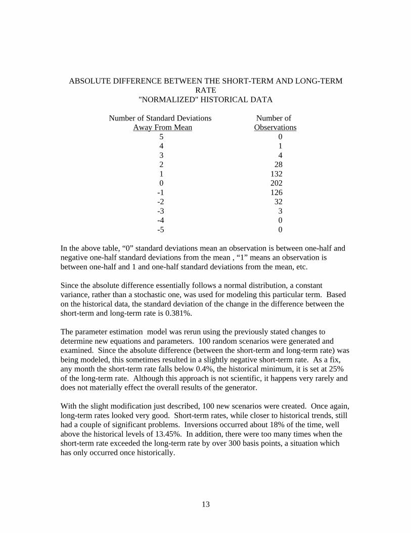
13

ABSOLUTE DIFFERENCE BETWEEN THE SHORT-TERM AND LONG-TERMRATE

"NORMALIZED" HISTORICAL DATA

Number of Standard Deviations Number ofAway From Mean Observations

5 0 4 1 3 4 2 28 1 132 0 202-1 126-2 32-3 3-4 0-5 0

In the above table, “0” standard deviations mean an observation is between one-half andnegative one-half standard deviations from the mean , “1” means an observation isbetween one-half and 1 and one-half standard deviations from the mean, etc.

Since the absolute difference essentially follows a normal distribution, a constantvariance, rather than a stochastic one, was used for modeling this particular term. Basedon the historical data, the standard deviation of the change in the difference between theshort-term and long-term rate is 0.381%.

The parameter estimation model was rerun using the previously stated changes todetermine new equations and parameters. 100 random scenarios were generated andexamined. Since the absolute difference (between the short-term and long-term rate) wasbeing modeled, this sometimes resulted in a slightly negative short-term rate. As a fix,any month the short-term rate falls below 0.4%, the historical minimum, it is set at 25%of the long-term rate. Although this approach is not scientific, it happens very rarely anddoes not materially effect the overall results of the generator.

With the slight modification just described, 100 new scenarios were created. Once again,long-term rates looked very good. Short-term rates, while closer to historical trends, stillhad a couple of significant problems. Inversions occurred about 18% of the time, wellabove the historical levels of 13.45%. In addition, there were too many times when theshort-term rate exceeded the long-term rate by over 300 basis points, a situation whichhas only occurred once historically.

14

After more experimentation, the problems were solved by strengthening the effect of themean reversion term (in the formula generating the excess of the short-term over thelong-term rate). The factor was increased from its derived level of 0.022 to 0.042. Noneof the other parameters or formulas were altered. (These are the equations in Section A.)

With the new mean reversion term, results were achieved which were excellent in manyareas and reasonable in the others. Long-term rates looked very good, as always. Theoccurrence of an inversion was reduced to 14.09% of the time, compared to the historicallevel of 13.45%. In addition, there were only 62 months, out of a possible 36,000, whenthe short-term rate exceeded the long-term rate by over 300 basis points (0.17% of thetime). This corresponds closely to reality, since it has only happened once in the 528-month period studied, or 0.19% of the time.

Section B has a series of tables which summarize the generated scenarios, and comparesthem to their historical (1951-1995) averages. The first table shows, in broad categories,the distribution of the long-term rate and the difference between the short and long-termrate on an absolute (non-normalized) basis. The second table shows, on a normalizedbasis (as previously defined), the distribution of the change in the long-term rate and thedistribution of the short-term minus the long-term rate. The final table shows thehistorical and generated distribution of interest rate inversions. For all tables, thehistorical numbers have been increased proportionately so that the number of historicalobservations and the number of generated observations are equal.

It should also be noted that the statistics in Section B are at least a little dependent on thestarting yield curve. In particular, a significantly different starting point could noticeablyimpact the non-normalized distribution of long-term rates. However, its impact on theother statistics would be minimal. It does not change any of the conclusions reachedabout the validity of the stochastic variance model.

The yield curve on which the statistics are based is given below:

TREASURY YIELD CURVE AS OF 9-30-96

3-Month: 5.14% 3-Year: 6.28% 10-Year: 6.72%6-Month: 5.37% 5-Year: 6.46% 20-Year: 7.05%1-Year: 5.71% 7-Year: 6.60% 30-Year: 6.93%2-Year: 6.10%

DERIVATION OF THE TREASURY YIELD CURVE

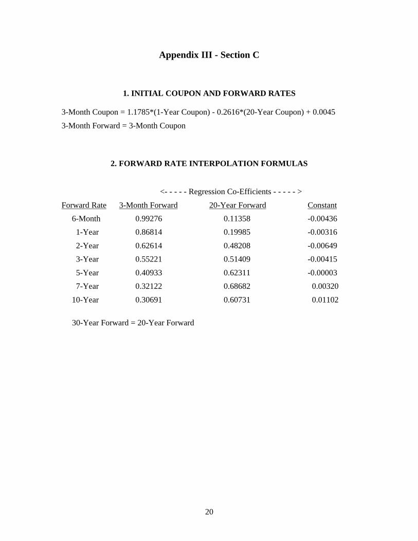
After the 1-year (short-term) and 20-year (long-term) coupon rates have been generated,the remainder of the treasury yield curve is derived from various interpolation anditerative formulas. First the 3-month treasury is calculated as a linear function of the 1-year and 20-year rates. The equation (given in Section C) comes from a linear regressionperformed on the monthly treasury coupon rates covering the period from March, 1977through May, 1997.

15

The 3-month and 20-year coupon rates serve as the starting point for calculating the othertreasury rates (6-month, 1-year, 2-year, 3-year, 5-year, 7-year, 10-year, and 30-year). Wedecided to interpolate using forward rates rather than coupon rates, in order to preventunintended and in some cases, unrealistic results.

The first thing that was done was convert the historical coupon-paying yield curves intohistorical forward curves. Since our data was limited to 10 points along the yield curve(listed above), forward rates were only calculated at the same 10 points. The keyassumption used in calculating the historical forwards is that forward rates remainconstant in between maturities. For example, the 21-year, 22-year,..., and 29-yearforward rates are all assumed equal to the 20-year forward. This is different than PTS,which uses linear interpolation to get at rates between maturities.

Linear regressions were performed on the calculated forward rates. Each forward ratewas represented as a linear function of the 3-month and 20-year forward. (The regressionequations are given in Section C.) Initially the 30-year forward was a linear function ofthe 3-month and 20-year forwards, just like the other rates. Unfortunately, the 30-yearregression equation produced very unrealistic results, so the simplifying assumption wasmade to set the 30-year forward equal to the 20-year forward.

Given the interpolation formulas and the generated 3-month and 20-year coupon rates,the remainder of the coupon yield curve is derived using an iterative process. The firststep is to set the 3-month forward rate equal to the 3-month coupon rate. A first estimateof the 20-year forward is then made. Given the 3-month and 20-year forwards, the otherforward rates are calculated using the regression equations in Section C. Once theforward curve has been generated, it is used to derive the corresponding coupon-payingcurve. If the derived 20-year coupon rate equals the previously generated 20-year couponrate, we have a “legitimate” treasury yield curve and the process stops. Otherwise,another estimate of the 20-year forward is made using a Newton-Raphson process, andthe iterations continue until the 20-year derived rate is equal to the 20-year generatedrate. This process is done for every year in which random interest rates are generated.

Underlying the entire process is the random number generator, which has been takendirectly from the book “Numerical Recipes in C”. For a given initial seed, the generatoralways produces the identical series of random numbers in identical order. This meansthat the random characteristics of the generated scenarios will be the same whatever theinitial yield curve. The characteristics of a scenario refers to the level of interest rates(high or low interest rate environment), and the shape of the yield curve (increasing, flat,or inverted).

16

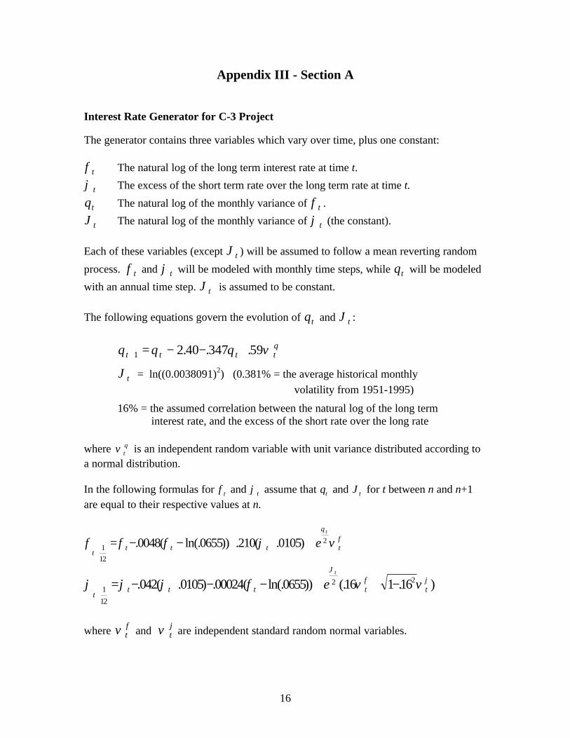
Appendix III - Section A

Interest Rate Generator for C-3 Project

The generator contains three variables which vary over time, plus one constant:

φt The natural log of the long term interest rate at time t.

ϕt The excess of the short term rate over the long term rate at time t.

θt The natural log of the monthly variance of φt .

ϑt The natural log of the monthly variance of ϕt (the constant).

Each of these variables (except ϑt ) will be assumed to follow a mean reverting random

process. φt and ϕt will be modeled with monthly time steps, while θt will be modeled

with an annual time step. ϑt is assumed to be constant.

The following equations govern the evolution of θt and ϑt :

θ θ θ ϖ θt t t t+ = − − +1 2 40 347 59. . .

ϑt = ln((0.0038091)2) (0.381% = the average historical monthly

volatility from 1951-1995)

16% = the assumed correlation between the natural log of the long term interest rate, and the excess of the short rate over the long rate

where ϖ θt is an independent random variable with unit variance distributed according to

a normal distribution.

In the following formulas for φt and ϕt assume that θt and ϑt for t between n and n+1are equal to their respective values at n.

φ φ φ ϕ ϖθ

φ

tt t t te

t

+= − − + + +1

12

20048 0655 210 0105. ( ln(. )) . ( . )

ϕ ϕ ϕ φ ϖ ϖϑ

φ ϕ

tt t t t te

t

+= − + − − + + −1

12

2 2042 0105 00024 0655 16 1 16. ( . ) . ( ln(. )) (. . )

where ϖ φt and ϖ ϕ

t are independent standard random normal variables.

17

Appendix III - Section B

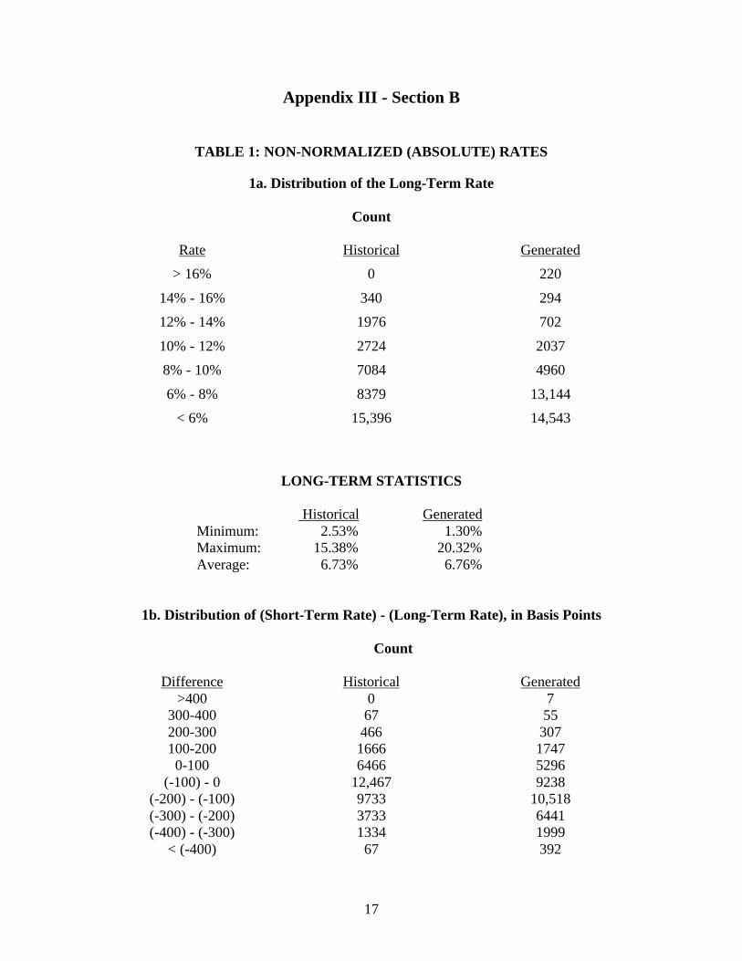
TABLE 1: NON-NORMALIZED (ABSOLUTE) RATES

1a. Distribution of the Long-Term Rate

Count

Rate Historical Generated

> 16% 0 220

14% - 16% 340 294

12% - 14% 1976 702

10% - 12% 2724 2037

8% - 10% 7084 4960

6% - 8% 8379 13,144

< 6% 15,396 14,543

LONG-TERM STATISTICS

Historical GeneratedMinimum: 2.53% 1.30%Maximum: 15.38% 20.32%Average: 6.73% 6.76%

1b. Distribution of (Short-Term Rate) - (Long-Term Rate), in Basis Points

Count

Difference Historical Generated>400 0 7

300-400 67 55200-300 466 307100-200 1666 17470-100 6466 5296

(-100) - 0 12,467 9238(-200) - (-100) 9733 10,518(-300) - (-200) 3733 6441(-400) - (-300) 1334 1999

< (-400) 67 392

18

SHORT-TERM MINUS LONG-TERM STATISTICS (IN BASIS POINTS)

Historical GeneratedMinimum: -423 -564Maximum: 368 477Average: -80 -109

19

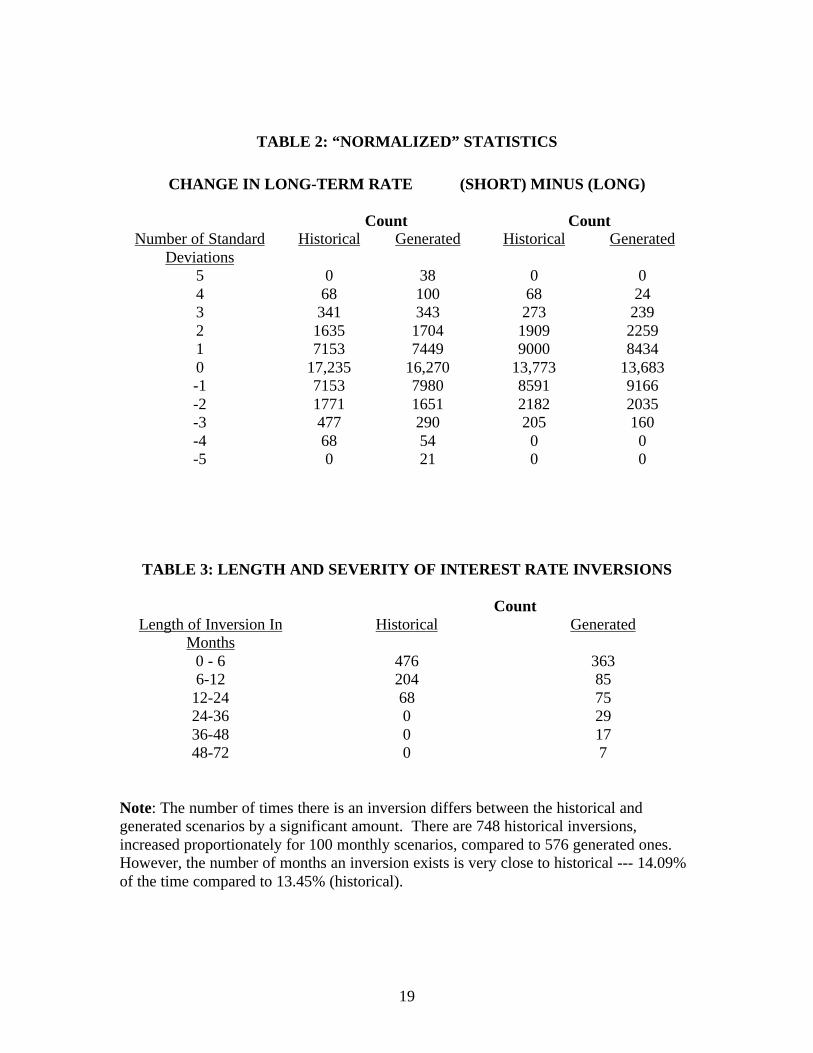
TABLE 2: “NORMALIZED” STATISTICS

CHANGE IN LONG-TERM RATE (SHORT) MINUS (LONG)

Count CountNumber of Standard

DeviationsHistorical Generated Historical Generated

5 0 38 0 04 68 100 68 243 341 343 273 2392 1635 1704 1909 22591 7153 7449 9000 84340 17,235 16,270 13,773 13,683-1 7153 7980 8591 9166-2 1771 1651 2182 2035-3 477 290 205 160-4 68 54 0 0-5 0 21 0 0

TABLE 3: LENGTH AND SEVERITY OF INTEREST RATE INVERSIONS

CountLength of Inversion In

MonthsHistorical Generated

0 - 6 476 3636-12 204 85

12-24 68 7524-36 0 2936-48 0 1748-72 0 7

Note: The number of times there is an inversion differs between the historical andgenerated scenarios by a significant amount. There are 748 historical inversions,increased proportionately for 100 monthly scenarios, compared to 576 generated ones.However, the number of months an inversion exists is very close to historical --- 14.09%of the time compared to 13.45% (historical).

20

Appendix III - Section C

1. INITIAL COUPON AND FORWARD RATES

3-Month Coupon = 1.1785*(1-Year Coupon) - 0.2616*(20-Year Coupon) + 0.0045

3-Month Forward = 3-Month Coupon

2. FORWARD RATE INTERPOLATION FORMULAS

<- - - - - Regression Co-Efficients - - - - - >

Forward Rate 3-Month Forward 20-Year Forward Constant

6-Month 0.99276 0.11358 -0.00436

1-Year 0.86814 0.19985 -0.00316

2-Year 0.62614 0.48208 -0.00649

3-Year 0.55221 0.51409 -0.00415

5-Year 0.40933 0.62311 -0.00003

7-Year 0.32122 0.68682 0.00320

10-Year 0.30691 0.60731 0.01102

30-Year Forward = 20-Year Forward

21

Appendix IV - AAA C-3 Pilot Testing: Selecting the 50 &12 ScenarioSubsets

Cash flow testing models developed in support of year-end 1996 Appointed Actuaryefforts were used to evaluate the new C-3 approach on a pilot basis. Models for sixblocks of in-force liabilities were tested for the following product types:

• Guaranteed Investment Contracts• Single Premium Immediate Annuities• Single Premium Deferred Annuities• Flexible Premium Deferred Annuities• Group Pensions - Reg. 128-Payable Annuities• Group Pension – IPG/Defined Benefit

Par Life insurance was also modeled, but didn’t generate a C-3 requirement, so it wasnot used in selecting scenario sets.

To evaluate whether the RBC measurement methodology was appropriately sensitive toalternative asset strategies (including some extreme ones), the liability portfolios wererun using a set of eight stylized investment strategies below. Besides strategies thatwould be considered to be well managed, the set includes portfolios with exposures toduration mismatch and portfolios with exposures to call-option risk.

• Non-callable A-rated Bonds – bullet (liability duration-matched)• Non-callable A-rated Bonds – ladder (liability duration-matched)• Non-callable A-rated Bonds – extreme bar-bell (liability duration-matched)• Non-callable A-rated Bonds – ladder (asset duration greater than liability by

three years)• Non-callable A-rated Bonds – ladder (asset duration less than liability by two

years)• Residential Mortgage Pass-Thrus (liability duration-matched - approximate)• CMOs: PAC tranche (liability duration-matched - approximate)• CMOs: support tranche (liability duration-matched - approximate)

The pilot testing consisted of running each of the 48 product type / stylized asset strategycombinations (48 Combinations) using the set of all interest rate scenarios. For each ofthe 48 Combinations, the accumulated statutory position was derived and captured foreach calendar year over the testing horizon for all 200 scenarios.

Selection of the Scenarios and the Optimal Number

The results from each of the 48 Combinations using the full 200 scenario set werecollected in a common database. Empirical analyses were performed to select a subset ofthe 200 scenarios such that this subset closely approximated the C-3 factors derived fromthe full 200-scenario set across the 48 Combinations.

22

In the end, 50 scenarios were selected. These scenarios can be thought of producing a C-3 factor result across a wide array of product/asset strategy combinations consistent withthe larger 200-scenario set. Alternatively, the 150 (75%) scenarios not selected can becharacterized as those not likely to generate a C-3 factor, and are generally more “level”and less volatile than the 50 selected. Thus, the formula used to derive the C-3 factorfrom the subset of 50 assumes that they come from a larger set of 200, and that testing theother 150 scenarios would not provide any material additional information adding littlevalue relative to the extra effort.

Selecting the Subset of 50

• For each of the 48 Product (6) & Asset Strategy (8) combinations, an “actual” C-3factor was developed using the full set of 200 scenarios. The C-3 factor for each ofthe 48 Product/Asset combinations was calculated by ordering the 200 scenarios fromworst-to-best using minimum surplus (a weighted average of the factors between the92nd percentile and the 98th percentile, centered at the 95th percentile, and including ½percentiles) as the criteria. Of the 200 scenarios, 83 of them contributed to at leastone of the 48 combination’s weighted-average C-3 factors.

• Assigning an ordinal number to the sorted (worst-to-best) scenarios within each of the48 combinations, a rank for each scenario across all combinations was determined.Sorting by rank, the 50 most frequent contributors to the calculation of all weighted-average C-3 factors were identified and an ordered, weighted-average C-3 factor wascalculated for each of the 48 combinations.

• The set of “50 worst” closely reproduces the “actual” weighted-average C-3 factor formost of the 48 Combinations. The exceptions in terms of absolute C-3 factordifference were: GIC Ladder-2, SPIA Barbell, SPIA Ladder+3, SPIA CMO-Supportand FPDA Barbell. These differences were deemed reasonable given that these fewcombinations had very high C-3 factors to start with, and thus the differences werenot considered problematic.

• In the same way, 20, 30 and 40 scenario subsets were selected and tested. Comparedto the 50-scenario set, there is a significant loss of “precision” that occurs when thenumber of scenarios is limited to 20 or 30 scenarios. The deterioration was lessgoing from 50 to 40 scenarios, but still enough that a 50 scenario subset was deemedto be a more appropriate subset for C-3 testing. (See Attachment X).

Selecting the Subset of 12

After selecting the 50-scenario subset, additional empirical studies were conducted todetermine if a yet smaller subset (10-20 scenarios) could be chosen from the 50 such thata C-3 factor result would be at least as conservative as using the 50-scenario subset. Theobjective was to pick a subset of the 50 such that the single worst (highest) C-3 factor ofthe subset was at least as great as the C-3 factor derived from the full 200 set. Thus, if a

23

company were to use this limited subset, their work effort might be reduced with thelikelihood of a more conservative C-3 factor.

Using a trial and error approach, a set of 12 scenarios was selected that met the objective.The analysis indicated the single worst result of the 12 scenarios produced an overlyconservative C-3 factor. After some experimentation, an approach was selected thatprovided a more reasonable result: the average of the second worst and third worst C-3factor, but not less than one-half the single worst factor from the subset. For the sample48 Combinations, using the 12 scenarios and the formula approach just describedproduced C-3 factors 1.5 to 2.5 times the full 200-scenario factor, averaging about 1.8times.

Two product/strategy combinations were merged to study the effects of aggregation. Forboth the 50-scenario subset and the 12-scenario subset, these studies yielded results thatwere consistent with the expected benefits of aggregation. The results for the 12-scenariosubset were also consistent with the level of conservatism found in the non-aggregated 48Combinations. This latter result provided further assurance that using the 12-scenariosubset would generate a more conservative result than the 50-scenario subset.

Attachment Y provides a pictorial perspective of the five-year rates across 30 years forthe 12-scenario subset.

Attachment Z provides some statistics related the 200-scenario set. The first page of theattachment contains the 50 scenarios selected to be used for C-3 testing. The first 12(shaded) are the subset of the 50 that can be used in the abbreviated testing. Notunexpectedly, the scenario statistic “scenario description” over the first 10 years has veryfew “levels” in the 50 and none in the 12. These “levels” are very prevalent in the 150scenarios not selected. This is consistent with the notion that more “C-3” information iscontained in the non-level scenarios.