Report of the American Academy of Actuaries’ Variable

Report of the American Academy of Actuaries’

Variable Annuity Reserve Work Group

Presented to the National Association of Insurance Commissioners’ Life and Health Actuarial Task Force

New York, NY – March 2004

The American Academy of Actuaries is the public policy organization for actuaries practicing in all specialties within the United States. A major purpose of the Academy is to act as the public information organization for the profession. The Academy is non-partisan and assists the public policy process through the presentation of clear and objective actuarial analysis. The Academy regularly prepares testimony for Congress, provides information to federal elected officials, comments on proposed federal regulations, and works closely with state officials on issues related to insurance. The Academy also develops and upholds actuarial standards of conduct, qualification and practice and the Code of Professional Conduct for all actuaries practicing in the United States.

Variable Annuity Reserve Work Group

Thomas A. Campbell, F.S.A., M.A.A.A., Chair James W. Lamson, F.S.A., M.A.A.A., Vice-Chair

Stephen J. Abels, F.S.A., M.A.A.A. Robert A. Brown, F.S.A., M.A.A.A. Richard A. Combs, F.S.A., M.A.A.A. Andrew D. Eastman, F.S.A., M.A.A.A. Larry M. Gorski, F.S.A., M.A.A.A. James R. Lodermeier, F.S.A., M.A.A.A.

John O'Sullivan, F.S.A., M.A.A.A. Edward L. Robbins, F.S.A., M.A.A.A. James F. Reiskytl, F.S.A., M.A.A.A. Keith A. Terry, F.S.A., M.A.A.A. Vincent Tsang, F.S.A., M.A.A.A. Van E. Villaruz, F.S.A., M.A.A.A.

The work group would also like to recognize the following individuals for their valuable input: Mike Akers, Rich Ash, Donna Claire, Allen Elstein, Jack Gies, Barbara Gold, Kerry Krantz, Barbara Lautzenheiser, Dennis Lauzon, Bob Meilander, Craig Morrow, Kory Olsen, Steve Preston, Max Rudolph, Scott Schneider, and Steven Sorrentino.

1

The VARWG would like to acknowledge the tireless work of Geoffrey H. Hancock and Robert F. Berendsen. The work group felt that their enormous efforts with the Academy’s Life Capital Adequacy Subcommittee’s (LCAS) C-3 Phase II RBC project made them the best candidates to develop a workable factor methodology, especially given the tight time frame required for completion. As part of their long-standing and continued involvement with the VARWG, Mr. Hancock and Mr. Berendsen volunteered for this work, but the methodology remains part of the collective work product of the LCAS and VARWG as part of its recommendation to the NAIC Life RBC Working Group. The VARWG would also like to thank Mercer Oliver Wyman, Mr. Hancock’s and Mr. Berendsen’s employer, for allowing them (as well as others from Mercer) to put in the time needed to complete this important project.

2

American Academy of Actuaries Variable Annuity Reserve Work Group

March 2004 Report

I. Background

The Variable Annuity Reserve Work Group (VARWG) was formed in January 2003 as a work group of the American Academy of Actuaries' Life Practice Council (LPC), drawing resources from the Life Capital Adequacy Subcommittee and the Life Valuation Subcommittee. Its charge is to examine issues surrounding the development of a reserve methodology for variable annuity products that uses the principles of the proposed Risk-Based Capital (RBC) C-3 Phase II approach. The VARWG is continuing to examine the effectiveness of such a methodology, and is identifying and commenting on regulatory and practicality issues. The work group is also working with the NAIC’s Life and Health Actuarial Task Force (LHATF) to develop the methodology and make recommendations on strategies to address any issues that have been identified or that may arise.

The reserve methodology being developed, if adopted, could be applicable to all variable annuity products. Such a methodology could replace, where appropriate, the application of Actuarial Guideline XXXIII to variable annuity contracts and totally replace Actuarial Guidelines XXXIV and XXXIXTPF

1FPT.

This report summarizes the work of the VARWG since the December 2003 NAIC meeting.

The VARWG is asking LHATF to resolve the issues raised in the December 2003 VARWG Report and expose the final proposal with the intent of adopting at the June 2004 LHATF meeting.

TP

1PT For purposes of this paragraph, it is important to note that no proposal has been made by the VARWG as to

whether the reserve methodology discussed in this report, if adopted, would apply to inforce contracts.

3

II. December NAIC Meeting

A. USummary of IssuesU

At the December NAIC meeting, it was recognized that the following issues required resolution:

1. The regulatory form of the recommended reserve methodology needs to be finalized.

2. Whether the proposed methodology should apply to all or a portion in-force contracts. If so, whether the application should be mandatory or elective.

3. The CTE level for the reserve methodology, which is currently set at CTE 65 in the draft actuarial guideline.

4. The appropriateness of the Alternative Methodology.

5. Whether a minimum reserve floor other than the PV of Annuitization Benefits is needed.

6. An acceptable method to approximate the reserve using results from a prior period (the "timing issue").

7. An acceptable method to allocate the resulting reserve to the contract level (the "allocation method"). Development of this method depends, in part, on the resolution to #5.

8. The effective date of the requirement.

9. Whether a phase-in of the new requirements is needed and, if so, how it should be structured.

10. Whether a method to dampen volatility is needed and, if so, how it should be structured.

Since that meeting, the VARWG identified an additional issue for which it has made a recommendation but is seeking input:

11. The treatment of Federal Income Taxes in the reserve methodology.

See Section III for more details on issue #11.

B. UCurrent DraftU

Based on prior feedback from LHATF, the VARWG drafted the current proposal in the form of an actuarial guideline that applies to all inforce business, and uses a CTE (65) standard for reserves (note that this does not represent a recommendation from VARWG regarding the level at which reserves should be established).

It is recognized that this does not necessarily reflect consensus by LHATF on these issues (in fact, several members of LHATF expressed views that varied from these, particularly on issues 1. and 2. above).

The current proposal was exposed by LHATF in December 2003 with the intent to seek comment from members of LHATF and other interested parties.

4

C. UNext Steps Agreed UponU

At the December LHATF meeting, the VARWG agreed to do the following:

1. Finalize the proposed methodology, based on input and direction from LHATF. 2. Work with LHATF to respond to comments from exposure. 3. Continue to analyze the impact of the reserve methodology on representative

products.

5

III. Update of Key Issues

A. UTimeline U

The timeline shown below was originally discussed during the September 2003 LHATF meeting. This timeline would allow a standard to be adopted by the NAIC by the end of 2004TPF

2FPT. It also provides for at least six months of exposure and comment.

In order to stay on this timeline, the VARWG is asking LHATF to expose the proposed Actuarial Guideline in this report for comment as soon as possible.

B. UAlternative FactorsU

For contracts with GMDBs only and no guaranteed living benefits, the draft guideline allows the option of determining reserves using an Alternative Methodology that allows application of factors as an alternative to using projections. At the December NAIC meeting, the VARWG reported that the Alternative Methodology was in the process of being developed for both reserve and the Risk-Based Capital C-3 Phase II project. We also reported that the methodology and the factors were first being developed for RBC and that factors for reserves would be developed once those were completed.

The methodology and factors for RBC were just recently completed. As of the date this report was completed, the instruction and documentation for the Alternative Methodology were being finalized. Factors for reserves are now being developed.

Appendix A contains the draft instruction and documentation for the Alternative Methodology. Although this document refers to RBC, the method as applied for reserves is the same. In addition, the updated draft Actuarial Guideline in Appendix H includes provisions for the Alternative Methodology within the reserve requirements.

TP

2PT Note that this does not necessarily mean that a new reserve standard will be in effect for year-end 2004. For

example, if the standard is adopted as an actuarial guideline, it is possible that the effective date might be later than 12/31/2004. Also, if the standard were adopted as either a model regulation or a revision to the model SVL, the standard would have to be adopted by individual states before it would be effective.

6

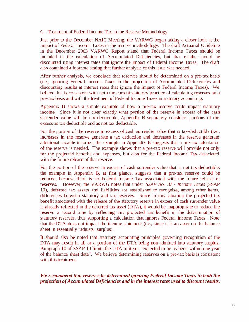
C. UTreatment of Federal Income Tax in the Reserve MethodologyU

Just prior to the December NAIC Meeting, the VARWG began taking a closer look at the impact of Federal Income Taxes in the reserve methodology. The draft Actuarial Guideline in the December 2003 VARWG Report stated that Federal Income Taxes should be included in the calculation of Accumulated Deficiencies, but that results should be discounted using interest rates that ignore the impact of Federal Income Taxes. The draft also contained a footnote stating that further analysis of this issue was needed.

After further analysis, we conclude that reserves should be determined on a pre-tax basis (i.e., ignoring Federal Income Taxes in the projection of Accumulated Deficiencies and discounting results at interest rates that ignore the impact of Federal Income Taxes). We believe this is consistent with both the current statutory practice of calculating reserves on a pre-tax basis and with the treatment of Federal Income Taxes in statutory accounting.

Appendix B shows a simple example of how a pre-tax reserve could impact statutory income. Since it is not clear exactly what portion of the reserve in excess of the cash surrender value will be tax deductible, Appendix B separately considers portions of the excess as tax deductible and as not tax deductible.

For the portion of the reserve in excess of cash surrender value that is tax-deductible (i.e., increases in the reserve generate a tax deduction and decreases in the reserve generate additional taxable income), the example in Appendix B suggests that a pre-tax calculation of the reserve is needed. The example shows that a pre-tax reserve will provide not only for the projected benefits and expenses, but also for the Federal Income Tax associated with the future release of that reserve.

For the portion of the reserve in excess of cash surrender value that is not tax-deductible, the example in Appendix B, at first glance, suggests that a pre-tax reserve could be reduced, because there is no Federal Income Tax associated with the future release of reserves. However, the VARWG notes that under SSAP No. 10 - Income Taxes (SSAP 10), deferred tax assets and liabilities are established to recognize, among other items, differences between statutory and tax reserves. Since in this situation the projected tax benefit associated with the release of the statutory reserve in excess of cash surrender value is already reflected in the deferred tax asset (DTA), it would be inappropriate to reduce the reserve a second time by reflecting this projected tax benefit in the determination of statutory reserves, thus supporting a calculation that ignores Federal Income Taxes. Note that the DTA does not impact the income statement (i.e., since it is an asset on the balance sheet, it essentially "adjusts" surplus).

It should also be noted that statutory accounting principles governing recognition of the DTA may result in all or a portion of the DTA being non-admitted into statutory surplus. Paragraph 10 of SSAP 10 limits the DTA to items "expected to be realized within one year of the balance sheet date". We believe determining reserves on a pre-tax basis is consistent with this treatment.

We recommend that reserves be determined ignoring Federal Income Taxes in both the projection of Accumulated Deficiencies and in the interest rates used to discount results.

7

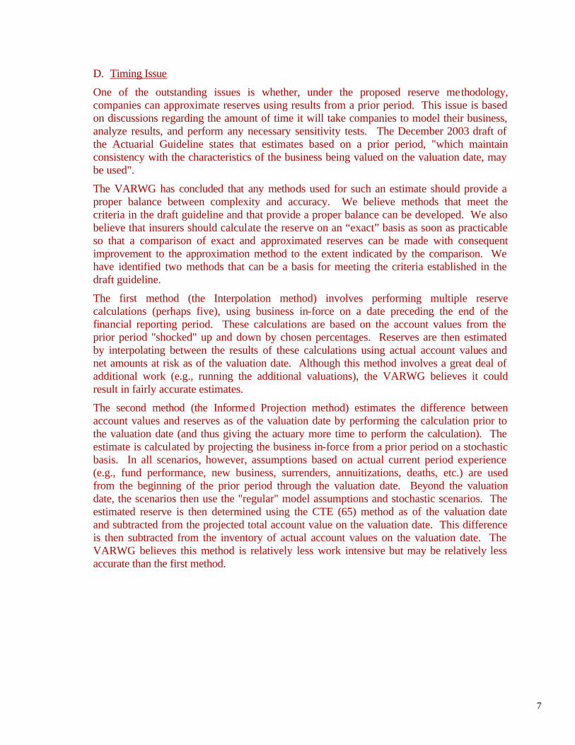
D. UTiming Issue U

One of the outstanding issues is whether, under the proposed reserve methodology, companies can approximate reserves using results from a prior period. This issue is based on discussions regarding the amount of time it will take companies to model their business, analyze results, and perform any necessary sensitivity tests. The December 2003 draft of the Actuarial Guideline states that estimates based on a prior period, "which maintain consistency with the characteristics of the business being valued on the valuation date, may be used".

The VARWG has concluded that any methods used for such an estimate should provide a proper balance between complexity and accuracy. We believe methods that meet the criteria in the draft guideline and that provide a proper balance can be developed. We also believe that insurers should calculate the reserve on an “exact” basis as soon as practicable so that a comparison of exact and approximated reserves can be made with consequent improvement to the approximation method to the extent indicated by the comparison. We have identified two methods that can be a basis for meeting the criteria established in the draft guideline.

The first method (the Interpolation method) involves performing multiple reserve calculations (perhaps five), using business in-force on a date preceding the end of the financial reporting period. These calculations are based on the account values from the prior period "shocked" up and down by chosen percentages. Reserves are then estimated by interpolating between the results of these calculations using actual account values and net amounts at risk as of the valuation date. Although this method involves a great deal of additional work (e.g., running the additional valuations), the VARWG believes it could result in fairly accurate estimates.

The second method (the Informed Projection method) estimates the difference between account values and reserves as of the valuation date by performing the calculation prior to the valuation date (and thus giving the actuary more time to perform the calculation). The estimate is calculated by projecting the business in-force from a prior period on a stochastic basis. In all scenarios, however, assumptions based on actual current period experience (e.g., fund performance, new business, surrenders, annuitizations, deaths, etc.) are used from the beginning of the prior period through the valuation date. Beyond the valuation date, the scenarios then use the "regular" model assumptions and stochastic scenarios. The estimated reserve is then determined using the CTE (65) method as of the valuation date and subtracted from the projected total account value on the valuation date. This difference is then subtracted from the inventory of actual account values on the valuation date. The VARWG believes this method is relatively less work intensive but may be relatively less accurate than the first method.

8

Appendix C describes the two methods in more detail. The VARWG believes there may be other acceptable methods that will emerge as practice develops.

We recommend that the language in the current draft of the guideline be retained and that the methods described in Appendix C be summarized in a practice note, along with any other acceptable methods that are developed.

We also recommend that companies using any approach to estimate reserves calculate actual reserves at a later time in order to analyze the accuracy of the approximation method chosen and to refine these methods based on this analysis.

9

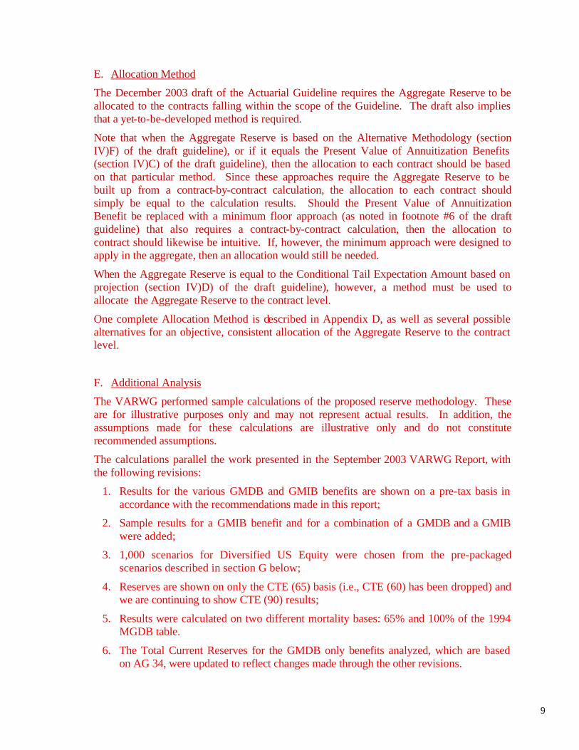
E. Allocation Method

The December 2003 draft of the Actuarial Guideline requires the Aggregate Reserve to be allocated to the contracts falling within the scope of the Guideline. The draft also implies that a yet-to-be-developed method is required.

Note that when the Aggregate Reserve is based on the Alternative Methodology (section IV)F) of the draft guideline), or if it equals the Present Value of Annuitization Benefits (section IV)C) of the draft guideline), then the allocation to each contract should be based on that particular method. Since these approaches require the Aggregate Reserve to be built up from a contract-by-contract calculation, the allocation to each contract should simply be equal to the calculation results. Should the Present Value of Annuitization Benefit be replaced with a minimum floor approach (as noted in footnote #6 of the draft guideline) that also requires a contract-by-contract calculation, then the allocation to contract should likewise be intuitive. If, however, the minimum approach were designed to apply in the aggregate, then an allocation would still be needed.

When the Aggregate Reserve is equal to the Conditional Tail Expectation Amount based on projection (section IV)D) of the draft guideline), however, a method must be used to allocate the Aggregate Reserve to the contract level.

One complete Allocation Method is described in Appendix D, as well as several possible alternatives for an objective, consistent allocation of the Aggregate Reserve to the contract level.

F. Additional Analysis

The VARWG performed sample calculations of the proposed reserve methodology. These are for illustrative purposes only and may not represent actual results. In addition, the assumptions made for these calculations are illustrative only and do not constitute recommended assumptions.

The calculations parallel the work presented in the September 2003 VARWG Report, with the following revisions:

1. Results for the various GMDB and GMIB benefits are shown on a pre-tax basis in accordance with the recommendations made in this report;

2. Sample results for a GMIB benefit and for a combination of a GMDB and a GMIB were added;

3. 1,000 scenarios for Diversified US Equity were chosen from the pre-packaged scenarios described in section G below;

4. Reserves are shown on only the CTE (65) basis (i.e., CTE (60) has been dropped) and we are continuing to show CTE (90) results;

5. Results were calculated on two different mortality bases: 65% and 100% of the 1994 MGDB table.

6. The Total Current Reserves for the GMDB only benefits analyzed, which are based on AG 34, were updated to reflect changes made through the other revisions.

10

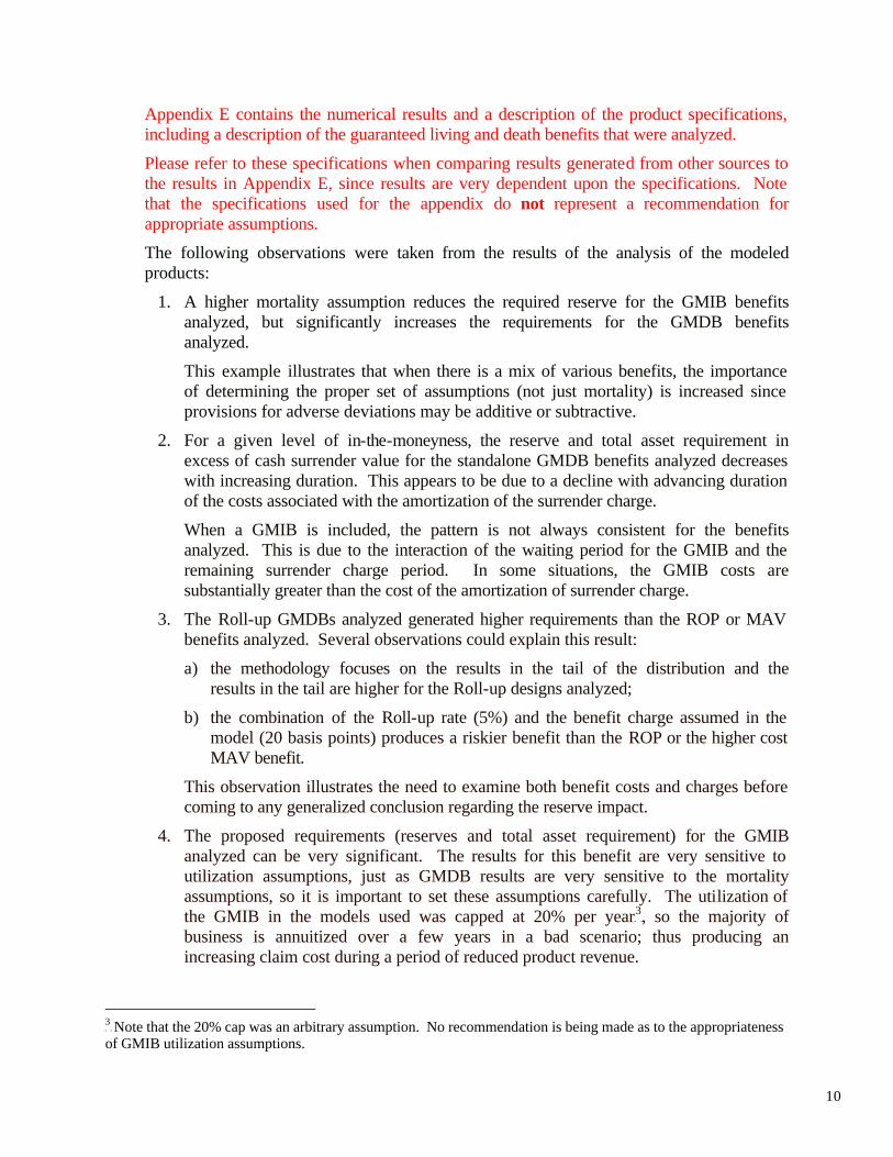
Appendix E contains the numerical results and a description of the product specifications, including a description of the guaranteed living and death benefits that were analyzed.

Please refer to these specifications when comparing results generated from other sources to the results in Appendix E, since results are very dependent upon the specifications. Note that the specifications used for the appendix do not represent a recommendation for appropriate assumptions.

The following observations were taken from the results of the analysis of the modeled products:

1. A higher mortality assumption reduces the required reserve for the GMIB benefits analyzed, but significantly increases the requirements for the GMDB benefits analyzed.

This example illustrates that when there is a mix of various benefits, the importance of determining the proper set of assumptions (not just mortality) is increased since provisions for adverse deviations may be additive or subtractive.

2. For a given level of in-the-moneyness, the reserve and total asset requirement in excess of cash surrender value for the standalone GMDB benefits analyzed decreases with increasing duration. This appears to be due to a decline with advancing duration of the costs associated with the amortization of the surrender charge.

When a GMIB is included, the pattern is not always consistent for the benefits analyzed. This is due to the interaction of the waiting period for the GMIB and the remaining surrender charge period. In some situations, the GMIB costs are substantially greater than the cost of the amortization of surrender charge.

3. The Roll-up GMDBs analyzed generated higher requirements than the ROP or MAV benefits analyzed. Several observations could explain this result:

a) the methodology focuses on the results in the tail of the distribution and the results in the tail are higher for the Roll-up designs analyzed;

b) the combination of the Roll-up rate (5%) and the benefit charge assumed in the model (20 basis points) produces a riskier benefit than the ROP or the higher cost MAV benefit.

This observation illustrates the need to examine both benefit costs and charges before coming to any generalized conclusion regarding the reserve impact.

4. The proposed requirements (reserves and total asset requirement) for the GMIB analyzed can be very significant. The results for this benefit are very sensitive to utilization assumptions, just as GMDB results are very sensitive to the mortality assumptions, so it is important to set these assumptions carefully. The utilization of the GMIB in the models used was capped at 20% per yearTPF

3FPT, so the majority of

business is annuitized over a few years in a bad scenario; thus producing an increasing claim cost during a period of reduced product revenue.

TP

3PT Note that the 20% cap was an arbitrary assumption. No recommendation is being made as to the appropriateness

of GMIB utilization assumptions.

11

Although the analysis was not performed at different ages, some would expect lower utilization and therefore lower reserves at younger ages (all other things being equal).

5. For the combination GMDB/GMIB product analyzed, the requirements are less than the sum of the separate requirements for the GMDB and GMIB (although higher than either benefit by itself). This synergy reflects the fact that the higher product revenue from both benefits is available to fund either benefit.

6. For the benefits analyzed, the requirements can dramatically increase as the benefit goes deeper into the money. For example, the Roll-up GMDB combined with GMIB product analyzed shows that the Total Asset Requirement in excess of cash surrender value at duration 9.5 increases from 7% of account value when the benefit is at-the-money to 27% of account value when the benefit is 40% in-the-money.

It is important to note that these observations may not hold true for other product designs or specifications.

G. Pre-Packaged Scenarios

The Academy's Life Capital Adequacy Subcommittee (LCAS) has developed a set of 10,000 stochastically generated scenarios for twelve asset classes with proper calibration of the diversified U.S. equity return distribution and appropriate correlations between the asset classes. The specifications for the development of these scenarios are contained in Appendix F. The scenarios themselves can be downloaded from the Academy’s website ( Thttp://www.actuary.org/life/phase2.htmT), along with a tool to help select a subset of the scenarios.

Appendix F of this report was originally presented in the December 2003 report titled Recommended Approach for Setting Regulatory Risk-Based Capital Requirements for Variable Products with Guarantees (Excluding Index Guarantees) from the LCAS.

H. Potential Methods to Dampen Volatility

There has been prior discussion about the period-to-period volatility of the results of the proposed methodologies for reserves and RBC, and the need for methods to dampen this volatility. The VARWG does not have a position on whether a method to dampen volatility is justified or necessary. We would like to offer the material in Appendix G to facilitate the discussion of this issue.

Appendix G of this report was originally presented in the September 2003 report titled Recommended Approach for Setting Regulatory Risk-Based Capital Requirements for Variable Products with Guarantees (Excluding Index Guarantees) from the LCAS.

12

I. Regulatory Form of the Recommended Reserve Methodology

During the February 18, 2004 LHATF conference call, there was a discussion regarding the regulatory form of the proposed reserve methodology. A part of that discussion involved the possibility of incorporating new reserve requirements under the scope of Section 9 of the NAIC Model Standard Valuation Law ("SVL"). A VARWG report entitled Promulgating the New Reserve Method for Variable Annuities was distributed for that call. The document was, however, a draft version of that report, which was developed for a LHATF conference call that took place prior to the September 2003 NAIC meeting (the VARWG regrets not realizing this prior to the February 18 call). The report was updated for the September 2003 meeting to incorporate the discussion on Section 9 of the SVL during that prior conference call.

Appendix H contains a reprint of the final version of the report, which appeared in the VARWG September 2003 Report, and is included to facilitate the discussion on the regulatory form.

J. Proposed Actuarial Guideline

As a result of the issues discussed above, several changes have been made to the draft Actuarial Guideline presented in December 2003. The updated draft Actuarial Guideline is presented in Appendix I. The following key modifications were made:

1. Changes to the treatment of Federal Income Tax in the reserve methodology, as discussed above, were incorporated throughout the draft guideline (particularly in Appendix 1).

2. A definition for Cash Surrender Value was added to Section III).

3. Details on the Alternative Methodology were added to Appendix 3.

4. It was clarified that companies could switch from determining the reserve using modeling to the Alternative Methodology with approval in Section IV).

5. A method to allocate the Aggregate Reserve to the contract level, as discussed above, was added to Appendix 5.

13

IV. Next Steps

The following are the areas on which the VARWG expects to focus going forward:

A. Recommend updates to the proposed methodology, based on input and direction from LHATF.

B. Finish calculating and distribute the Alternative Methodology.

C. Work with LHATF to respond to comments from exposure.

D. Continue to analyze the impact of the reserve methodology on representative products.

E. Analyze and comment on the standard scenario proposal. We will also incorporate the standard scenario into the proposed standard if LHATF wishes us to do so.

F. Where appropriate, identify the need for professional and practical guidance and begin the process to help develop the guidance.

The VARWG plans to continue to update LHATF on its progress at future NAIC meetings and on interim conference calls.

Appendix A - Alternative Methodology for GMDB by Geoffrey H. Hancock

Background The AAA Life Capital Adequacy Subcommittee (“LCAS”) issued a report entitled “Recommended Approach for Setting Regulatory Risk-Based Capital Requirements for Variable Products with Guarantees (Excluding Index Guarantees)” in December 2002 that recommends implementing “C3 Phase II RBC” to address both the interest rate and equity risk associated with variable products with guarantees. The LCAS issued a revised report September 2003. While some issues have been clarified or removed from scope, the methodology and proposals remain substantially unchanged.

Notably, the LCAS recommendation permits companies with “guaranteed minimum death benefits only” products to choose between scenario testing or a factor approach, provided they have not used scenario testing in previous years. Other guarantees (e.g., so-called “guaranteed living benefits” – or VAGLBs – that depend on the survival and deliberate/elective action of the policyholder either through persistency or option exercise) require scenario testing. The factor-based approach – referred to as the “Alternative Method” – was not described in detail, but the report states that:

“A company may choose to develop capital requirements for Variable Annuity contracts having GMDBs and not having VAGLBs, by using the tables from Appendix 8 … of this report instead of using scenario testing if it hasn’t used scenario testing for this purpose in previous years. Companies are encouraged to develop models to allow scenario testing for this purpose. Once the stochastic modeling methodology is used for this purpose, the option to use Appendix 8 factors is no longer available. Other covered benefits must be evaluated by scenario testing.”

However, Appendix 8 was not included in the LCAS Dec 2002 report or in the September 2003 update, although considerable testing and results had been made public through the AAA LCAS electronic mail list. This document is intended to describe the Alternative Methodology in significant detail and eventually comprise Appendix 8. Upon the completion of final testing, tables of factors (and associated formulas) will be provided. To assist the Variable Annuity Reserve Working Group (“VARWG”), factors will be developed using the Conditional Tail Expectation (“CTE”) risk measure at two confidence levels: 0.65 and 0.90. The former will use pre-tax discount rates and ignore income taxes.

General

1. It is expected that the Alternative Methodology will be applied on a policy-by-policy basis (i.e., seriatim). If the company adopts a cell-based approach, only materially similar contracts should be grouped together. Specifically, all policies comprising a “cell” must display substantially similar characteristics for those attributes expected to affect risk-based capital (e.g., definition of guaranteed benefits, attained age, policy duration, years-to-maturity, market-to-guaranteed value, asset mix, etc.).

2. Under the LCAS recommendation (Sept 2003), RBC is defined as the “Total Asset Requirement” (as determined by stochastic modeling using the CTE90 risk measure) less actual statement reserves held in respect of the guarantees. The Alternative Methodology determines the Total Asset Requirement (“TAR”)

APPENDIX A

Alternative Methodology for GMDB – Version 10 Page 2 of 29

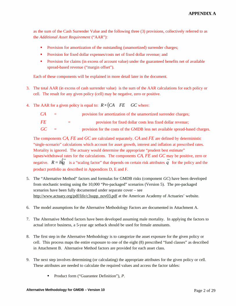
as the sum of the Cash Surrender Value and the following three (3) provisions, collectively referred to as the Additional Asset Requirement (“AAR”):

§ Provision for amortization of the outstanding (unamortized) surrender charges;

§ Provision for fixed dollar expenses/costs net of fixed dollar revenue; and

§ Provision for claims (in excess of account value) under the guaranteed benefits net of available spread-based revenue (“margin offset”).

Each of these components will be explained in more detail later in the document.

3. The total AAR (in excess of cash surrender value) is the sum of the AAR calculations for each policy or cell. The result for any given policy (cell) may be negative, zero or positive.

4. The AAR for a given policy is equal to: ( ) GCFECAR ++× where:

CA = provision for amortization of the unamortized surrender charges;

FE = provision for fixed dollar costs less fixed dollar revenue;

GC = provision for the costs of the GMDB less net available spread-based charges.

The components CA, FE and GC are calculated separately. CA and FE are defined by deterministic “single-scenario” calculations which account for asset growth, interest and inflation at prescribed rates. Mortality is ignored. The actuary would determine the appropriate “prudent best estimate” lapses/withdrawal rates for the calculations. The components CA, FE and GC may be positive, zero or

negative. ( )θ~

hR = is a “scaling factor” that depends on certain risk attributes θ~ for the policy and the

product portfolio as described in Appendices D, E and F.

5. The “Alternative Method” factors and formulas for GMDB risks (component GC) have been developed from stochastic testing using the 10,000 “Pre-packaged” scenarios (Version 5). The pre-packaged scenarios have been fully documented under separate cover – see Thttp://www.actuary.org/pdf/life/c3supp_nov03.pdfT at the American Academy of Actuaries’ website.

6. The model assumptions for the Alternative Methodology Factors are documented in Attachment A.

7. The Alternative Method factors have been developed assuming male mortality. In applying the factors to actual inforce business, a 5-year age setback should be used for female annuitants.

8. The first step in the Alternative Methodology is to categorize the asset exposure for the given policy or cell. This process maps the entire exposure to one of the eight (8) prescribed “fund classes” as described in Attachment B. Alternative Method factors are provided for each asset class.

9. The next step involves determining (or calculating) the appropriate attributes for the given policy or cell. These attributes are needed to calculate the required values and access the factor tables:

§ Product form (“Guarantee Definition”), P.

APPENDIX A


§ Adjustment to guaranteed value upon partial withdrawal (“GMDB Adjustment”), A.

§ Fund class, F.

§ Attained age of the annuitant, X.

§ Policy duration since issue, D.

§ Ratio of account value to guaranteed value, φ.

§ Total account charges, M.

Other required policy values include:

§ Account value, AV.

§ Current guaranteed minimum death benefit, GMDB.

§ Net deposit value (sum of deposits less sum of withdrawals), NetDeposits TPF

4FPT.

§ Net spread available to fund guaranteed benefits (“margin offset”), α.

10. GMDB may alternatively be denoted by GV in this document. The total account charges (“M”) should include all amounts assessed against policyholder accounts, expressed as a level spread per year (in basis points). This quantity is called the Management Expense Ratio (“MER”) and is defined as the average amount (in dollars) charged against policyholder funds in a given year divided by average account value. Normally, the MER would vary by fund class and be the sum of investment management fees, mortality & expense charges, guarantee fees/risk premiums, etc. The spread available to fund the GMDB costs (“margin offset”, denoted by α) should be net of spread-based costs and expenses (e.g., net of maintenance expenses, investment management fees, trailer commissions, etc.). Attachment H provides an example of how to determine M and α for a sample contract. ‘Time-to-maturity’ is uniquely defined in the factor modeling by T = 95 − X. Net deposits are used in determining benefit caps under the GMDB Roll-up and EDB designs.

11. The GMDB definition for a given policy/cell may not exactly correspond to those provided. In some cases, it may be reasonable to use the factors/formulas for a different product form (e.g., for a “roll-up” GMDB policy near or beyond the maximum reset age or amount, the company should use the “return-of-premium” GMDB factors/formulas, possibly adjusting the guaranteed value to reflect further resets, if any). In other cases, the company might determine the RBC based on two different guarantee definitions and interpolate the results to obtain an appropriate value for the given policy/cell. However, if the policy form (definition of the guaranteed benefit) is sufficiently different from those provided and there is no practical or obvious way to obtain a good result from the prescribed factors/formulas, the company must select one of the following options:

a) Model the “C3 Phase II RBC” using stochastic projections according to the approved methodology;

b) Select factors/formulas from the prescribed set such that the values obtained conservatively estimate the required capital; or

TP

4PT Net deposits are required only for certain policy forms (e.g., when the guaranteed benefit is capped as a multiple of net policy contributions).

APPENDIX A


c) Calculate company-specific factors or adjustments to the published factors based on stochastic testing of its actual business. This option is described more fully in Attachment I.

12. The actuary must decide if existing risk transfer arrangements or asset/liability management (“A/LM”) strategies (e.g., hedging) can be accommodated by a straight-forward adjustment to the factors and formulas (e.g., quota-share reinsurance without caps, floors or sliding scales would normally be reflected by a simple pro-rata adjustment to the “gross” GC results). For more complicated forms of reinsurance, and typically for A/LM strategies, the company will need to justify any adjustments or approximations by stochastic modeling. However, this modeling need not be performed on the whole portfolio, but can be undertaken on an appropriate set of representative policies. See Attachment I for more details.

APPENDIX A


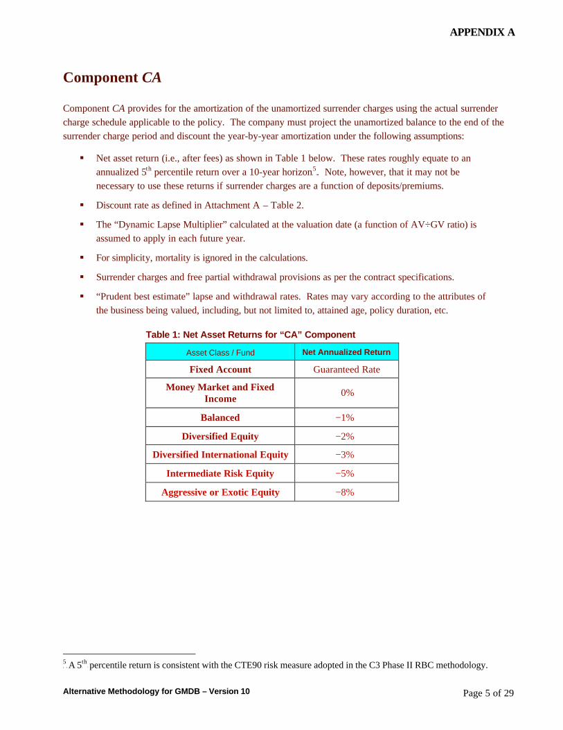
Component CA

Component CA provides for the amortization of the unamortized surrender charges using the actual surrender charge schedule applicable to the policy. The company must project the unamortized balance to the end of the surrender charge period and discount the year-by-year amortization under the following assumptions:

§ Net asset return (i.e., after fees) as shown in Table 1 below. These rates roughly equate to an annualized 5P

thP percentile return over a 10-year horizonTPF

5FPT. Note, however, that it may not be

necessary to use these returns if surrender charges are a function of deposits/premiums.

§ Discount rate as defined in Attachment A – Table 2.

§ The “Dynamic Lapse Multiplier” calculated at the valuation date (a function of AV÷GV ratio) is assumed to apply in each future year.

§ For simplicity, mortality is ignored in the calculations.

§ Surrender charges and free partial withdrawal provisions as per the contract specifications.

§ “Prudent best estimate” lapse and withdrawal rates. Rates may vary according to the attributes of the business being valued, including, but not limited to, attained age, policy duration, etc.

Table 1: Net Asset Returns for “CA” Component

Asset Class / Fund Net Annualized Return

Fixed Account Guaranteed Rate

Money Market and Fixed Income

0%

Balanced −1%

Diversified Equity −2%

Diversified International Equity −3%

Intermediate Risk Equity −5%

Aggressive or Exotic Equity −8%

TP

5PT A 5 P

thP percentile return is consistent with the CTE90 risk measure adopted in the C3 Phase II RBC methodology.

APPENDIX A


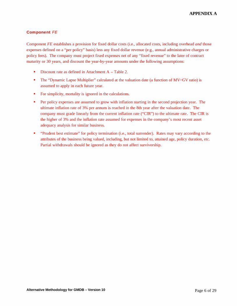
Component FE

Component FE establishes a provision for fixed dollar costs (i.e., allocated costs, including overhead and those expenses defined on a “per policy” basis) less any fixed dollar revenue (e.g., annual administrative charges or policy fees). The company must project fixed expenses net of any “fixed revenue” to the later of contract maturity or 30 years, and discount the year-by-year amounts under the following assumptions:

§ Discount rate as defined in Attachment A – Table 2.

§ The “Dynamic Lapse Multiplier” calculated at the valuation date (a function of MV÷GV ratio) is assumed to apply in each future year.

§ For simplicity, mortality is ignored in the calculations.

§ Per policy expenses are assumed to grow with inflation starting in the second projection year. The ultimate inflation rate of 3% per annum is reached in the 8th year after the valuation date. The company must grade linearly from the current inflation rate (“CIR”) to the ultimate rate. The CIR is the higher of 3% and the inflation rate assumed for expenses in the company’s most recent asset adequacy analysis for similar business.

§ “Prudent best estimate” for policy termination (i.e., total surrender). Rates may vary according to the attributes of the business being valued, including, but not limited to, attained age, policy duration, etc. Partial withdrawals should be ignored as they do not affect survivorship.

APPENDIX A


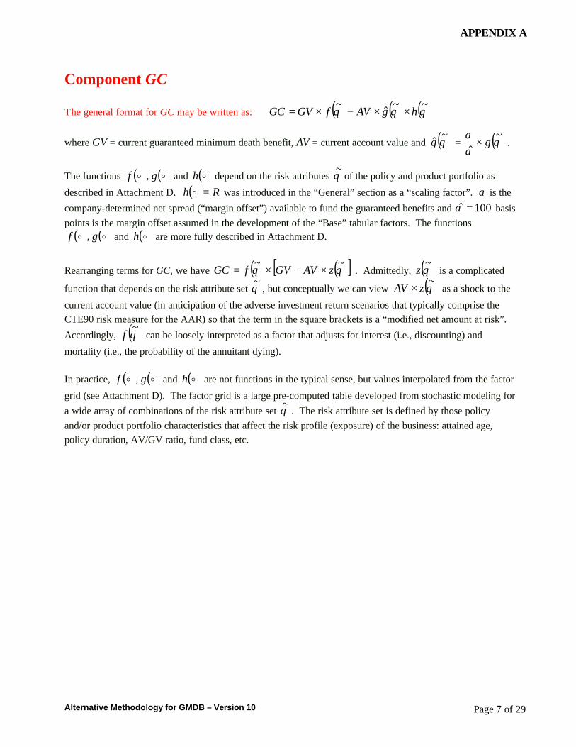
Component GC

The general format for GC may be written as: ( ) ( ) ( )θθθ~~ˆ~

hgAVfGVGC ××−×=

where GV = current guaranteed minimum death benefit, AV = current account value and ( )θ~

g = ( )θαα ~ˆ

g× .

The functions ( )of , ( )og and ( )oh depend on the risk attributes θ~ of the policy and product portfolio as

described in Attachment D. ( ) Rh =o was introduced in the “General” section as a “scaling factor”. α is the

company-determined net spread (“margin offset”) available to fund the guaranteed benefits and 100ˆ =α basis points is the margin offset assumed in the development of the “Base” tabular factors. The functions

( )of , ( )og and ( )oh are more fully described in Attachment D.

Rearranging terms for GC, we have ( ) ( )[ ]θθ~~

zAVGVfGC ×−×= . Admittedly, ( )θ~

z is a complicated

function that depends on the risk attribute set θ~ , but conceptually we can view ( )θ~

zAV × as a shock to the

current account value (in anticipation of the adverse investment return scenarios that typically comprise the CTE90 risk measure for the AAR) so that the term in the square brackets is a “modified net amount at risk”.

Accordingly, ( )θ~

f can be loosely interpreted as a factor that adjusts for interest (i.e., discounting) and

mortality (i.e., the probability of the annuitant dying).

In practice, ( )of , ( )og and ( )oh are not functions in the typical sense, but values interpolated from the factor

grid (see Attachment D). The factor grid is a large pre-computed table developed from stochastic modeling for a wide array of combinations of the risk attribute set θ~ . The risk attribute set is defined by those policy and/or product portfolio characteristics that affect the risk profile (exposure) of the business: attained age, policy duration, AV/GV ratio, fund class, etc.

APPENDIX A


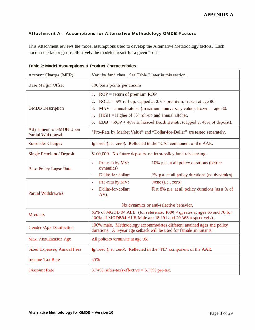
Attachment A – Assumptions for Alternative Methodology GMDB Factors

This Attachment reviews the model assumptions used to develop the Alternative Methodology factors. Each node in the factor grid is effectively the modeled result for a given “cell”.

Table 2: Model Assumptions & Product Characteristics

Account Charges (MER) Vary by fund class. See Table 3 later in this section.

Base Margin Offset 100 basis points per annum

GMDB Description

1. ROP = return of premium ROP.

2. ROLL = 5% roll-up, capped at 2.5 × premium, frozen at age 80.

3. MAV = annual ratchet (maximum anniversary value), frozen at age 80. 4. HIGH = Higher of 5% roll-up and annual ratchet.

5. EDB = ROP + 40% Enhanced Death Benefit (capped at 40% of deposit).

Adjustment to GMDB Upon Partial Withdrawal

“Pro-Rata by Market Value” and “Dollar-for-Dollar” are tested separately.

Surrender Charges Ignored (i.e., zero). Reflected in the “CA” component of the AAR.

Single Premium / Deposit $100,000. No future deposits; no intra-policy fund rebalancing.

Base Policy Lapse Rate • Pro-rata by MV: 10% p.a. at all policy durations (before

dynamics) • Dollar-for-dollar: 2% p.a. at all policy durations (no dynamics)

Partial Withdrawals

• Pro-rata by MV: None (i.e., zero)

• Dollar-for-dollar: Flat 8% p.a. at all policy durations (as a % of AV).

No dynamics or anti-selective behavior.

Mortality 65% of MGDB 94 ALB (for reference, 1000 × qBxB rates at ages 65 and 70 for 100% of MGDB94 ALB Male are 18.191 and 29.363 respectively).

Gender /Age Distribution 100% male. Methodology accommodates different attained ages and policy durations. A 5-year age setback will be used for female annuitants.

Max. Annuitization Age All policies terminate at age 95.

Fixed Expenses, Annual Fees Ignored (i.e., zero). Reflected in the “FE” component of the AAR.

Income Tax Rate 35%

Discount Rate 3.74% (after-tax) effective = 5.75% pre-tax.

APPENDIX A


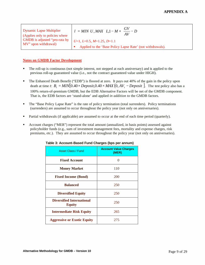
Dynamic Lapse Multiplier (Applies only to policies where GMDB is adjusted “pro-rata by MV” upon withdrawal)

−×−= D

AVGV

MLMAXUMIN 1,,λ

U=1, L=0.5, M=1.25, D=1.1

§ Applied to the ‘Base Policy Lapse Rate’ (not withdrawals).

Notes on GMDB Factor Development § The roll-up is continuous (not simple interest, not stepped at each anniversary) and is applied to the

previous roll-up guaranteed value (i.e., not the contract guaranteed value under HIGH).

§ The Enhanced Death Benefit (“EDB”) is floored at zero. It pays out 40% of the gain in the policy upon death at time t: ( )[ ]DepositAVMAXDepositMINB tt −××= ,040.0,40.0 . The test policy also has a 100% return-of-premium GMDB, but the EDB Alternative Factors will be net of the GMDB component. That is, the EDB factors are ‘stand-alone’ and applied in addition to the GMDB factors.

§ The “Base Policy Lapse Rate” is the rate of policy termination (total surrenders). Policy terminations (surrenders) are assumed to occur throughout the policy year (not only on anniversaries).

§ Partial withdrawals (if applicable) are assumed to occur at the end of each time period (quarterly).

§ Account charges (“MER”) represent the total amount (annualized, in basis points) assessed against policyholder funds (e.g., sum of investment management fees, mortality and expense charges, risk premiums, etc.). They are assumed to occur throughout the policy year (not only on anniversaries).

Table 3: Account-Based Fund Charges (bps per annum)

Asset Class / Fund Account Value Charges

(MER)

Fixed Account 0

Money Market 110

Fixed Income (Bond) 200

Balanced 250

Diversified Equity 250

Diversified International Equity

250

Intermediate Risk Equity 265

Aggressive or Exotic Equity 275

APPENDIX A


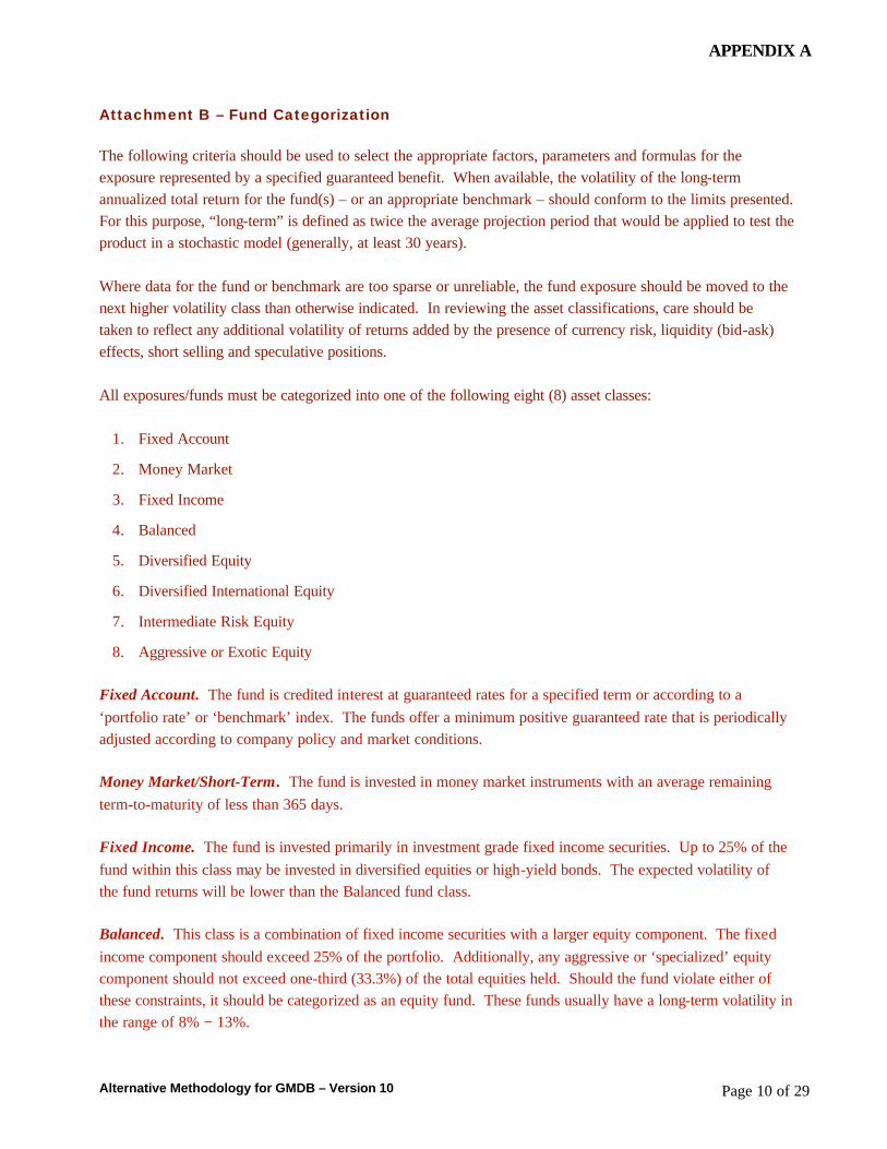
Attachment B – Fund Categorization

The following criteria should be used to select the appropriate factors, parameters and formulas for the exposure represented by a specified guaranteed benefit. When available, the volatility of the long-term annualized total return for the fund(s) – or an appropriate benchmark – should conform to the limits presented. For this purpose, “long-term” is defined as twice the average projection period that would be applied to test the product in a stochastic model (generally, at least 30 years).

Where data for the fund or benchmark are too sparse or unreliable, the fund exposure should be moved to the next higher volatility class than otherwise indicated. In reviewing the asset classifications, care should be taken to reflect any additional volatility of returns added by the presence of currency risk, liquidity (bid-ask) effects, short selling and speculative positions.

All exposures/funds must be categorized into one of the following eight (8) asset classes:

1. Fixed Account

2. Money Market

3. Fixed Income

4. Balanced

5. Diversified Equity

6. Diversified International Equity

7. Intermediate Risk Equity

8. Aggressive or Exotic Equity

Fixed Account. The fund is credited interest at guaranteed rates for a specified term or according to a ‘portfolio rate’ or ‘benchmark’ index. The funds offer a minimum positive guaranteed rate that is periodically adjusted according to company policy and market conditions.

Money Market/Short-Term. The fund is invested in money market instruments with an average remaining term-to-maturity of less than 365 days.

Fixed Income. The fund is invested primarily in investment grade fixed income securities. Up to 25% of the fund within this class may be invested in diversified equities or high-yield bonds. The expected volatility of the fund returns will be lower than the Balanced fund class.

Balanced. This class is a combination of fixed income securities with a larger equity component. The fixed income component should exceed 25% of the portfolio. Additionally, any aggressive or ‘specialized’ equity component should not exceed one-third (33.3%) of the total equities held. Should the fund violate either of these constraints, it should be categorized as an equity fund. These funds usually have a long-term volatility in the range of 8% − 13%.

APPENDIX A


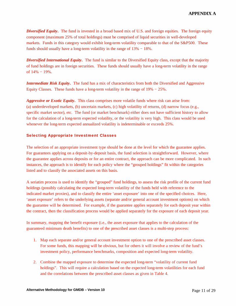
Diversified Equity. The fund is invested in a broad based mix of U.S. and foreign equities. The foreign equity component (maximum 25% of total holdings) must be comprised of liquid securities in well-developed markets. Funds in this category would exhibit long-term volatility comparable to that of the S&P500. These funds should usually have a long-term volatility in the range of 13% − 18%.

Diversified International Equity. The fund is similar to the Diversified Equity class, except that the majority of fund holdings are in foreign securities. These funds should usually have a long-term volatility in the range of 14% − 19%.

Intermediate Risk Equity. The fund has a mix of characteristics from both the Diversified and Aggressive Equity Classes. These funds have a long-term volatility in the range of 19% − 25%.

Aggressive or Exotic Equity. This class comprises more volatile funds where risk can arise from: (a) underdeveloped markets, (b) uncertain markets, (c) high volatility of returns, (d) narrow focus (e.g., specific market sector), etc. The fund (or market benchmark) either does not have sufficient history to allow for the calculation of a long-term expected volatility, or the volatility is very high. This class would be used whenever the long-term expected annualized volatility is indeterminable or exceeds 25%.

Selecting Appropriate Investment Classes

The selection of an appropriate investment type should be done at the level for which the guarantee applies. For guarantees applying on a deposit-by-deposit basis, the fund selection is straightforward. However, where the guarantee applies across deposits or for an entire contract, the approach can be more complicated. In such instances, the approach is to identify for each policy where the “grouped holdings” fit within the categories listed and to classify the associated assets on this basis.

A seriatim process is used to identify the “grouped” fund holdings, to assess the risk profile of the current fund holdings (possibly calculating the expected long-term volatility of the funds held with reference to the indicated market proxies), and to classify the entire ‘asset exposure’ into one of the specified choices. Here, ‘asset exposure’ refers to the underlying assets (separate and/or general account investment options) on which the guarantee will be determined. For example, if the guarantee applies separately for each deposit year within the contract, then the classification process would be applied separately for the exposure of each deposit year.

In summary, mapping the benefit exposure (i.e., the asset exposure that applies to the calculation of the guaranteed minimum death benefits) to one of the prescribed asset classes is a multi-step process:

1. Map each separate and/or general account investment option to one of the prescribed asset classes. For some funds, this mapping will be obvious, but for others it will involve a review of the fund’s investment policy, performance benchmarks, composition and expected long-term volatility.

2. Combine the mapped exposure to determine the expected long-term “volatility of current fund holdings”. This will require a calculation based on the expected long-term volatilities for each fund and the correlations between the prescribed asset classes as given in Table 4.

APPENDIX A


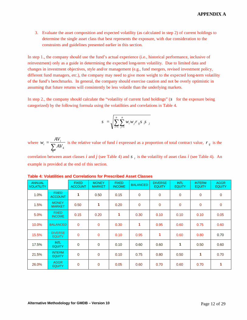
3. Evaluate the asset composition and expected volatility (as calculated in step 2) of current holdings to determine the single asset class that best represents the exposure, with due consideration to the constraints and guidelines presented earlier in this section.

In step 1., the company should use the fund’s actual experience (i.e., historical performance, inclusive of reinvestment) only as a guide in determining the expected long-term volatility. Due to limited data and changes in investment objectives, style and/or management (e.g., fund mergers, revised investment policy, different fund managers, etc.), the company may need to give more weight to the expected long-term volatility of the fund’s benchmarks. In general, the company should exercise caution and not be overly optimistic in assuming that future returns will consistently be less volatile than the underlying markets.

In step 2., the company should calculate the “volatility of current fund holdings” (σ for the exposure being categorized) by the following formula using the volatilities and correlations in Table 4.

∑∑= =

=n

i

n

jjiijji ww

1 1

σσρσ

where ∑

=

kk

ii AV

AVw is the relative value of fund i expressed as a proportion of total contract value, ijρ is the

correlation between asset classes i and j (see Table 4) and iσ is the volatility of asset class i (see Table 4). An

example is provided at the end of this section.

Table 4: Volatilities and Correlations for Prescribed Asset Classes

ANNUAL VOLATILITY

FIXED ACCOUNT

MONEY MARKET

FIXED INCOME BALANCED

DIVERSE EQUITY

INTL EQUITY

INTERM EQUITY

AGGR EQUITY

1.0% FIXED ACCOUNT

1 0.50 0.15 0 0 0 0 0

1.5% MONEY MARKET 0.50 1 0.20 0 0 0 0 0

5.0% FIXED INCOME 0.15 0.20 1 0.30 0.10 0.10 0.10 0.05

10.0% BALANCED 0 0 0.30 1 0.95 0.60 0.75 0.60

15.5% DIVERSE EQUITY 0 0 0.10 0.95 1 0.60 0.80 0.70

17.5% INTL EQUITY 0 0 0.10 0.60 0.60 1 0.50 0.60

21.5% INTERM EQUITY 0 0 0.10 0.75 0.80 0.50 1 0.70

26.0% AGGR EQUITY 0 0 0.05 0.60 0.70 0.60 0.70 1

APPENDIX A


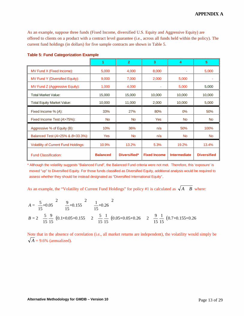
As an example, suppose three funds (Fixed Income, diversified U.S. Equity and Aggressive Equity) are offered to clients on a product with a contract level guarantee (i.e., across all funds held within the policy). The current fund holdings (in dollars) for five sample contracts are shown in Table 5.

Table 5: Fund Categorization Example

1 2 3 4 5

MV Fund X (Fixed Income): 5,000 4,000 8,000 - 5,000

MV Fund Y (Diversified Equity): 9,000 7,000 2,000 5,000 -

MV Fund Z (Aggressive Equity): 1,000 4,000 - 5,000 5,000

Total Market Value: 15,000 15,000 10,000 10,000 10,000

Total Equity Market Value: 10,000 11,000 2,000 10,000 5,000

Fixed Income % (A): 33% 27% 80% 0% 50%

Fixed Income Test (A>75%): No No Yes No No

Aggressive % of Equity (B): 10% 36% n/a 50% 100%

Balanced Test (A>25% & B<33.3%): Yes No n/a No No

Volatility of Current Fund Holdings: 10.9% 13.2% 5.3% 19.2% 13.4%

Fund Classification: Balanced Diversified* Fixed Income Intermediate Diversified

* Although the volatility suggests “Balanced Fund”, the Balanced Fund criteria were not met. Therefore, this ‘exposure’ is

moved “up” to Diversified Equity. For those funds classified as Diversified Equity, additional analysis would be required to

assess whether they should be instead designated as “Diversified International Equity”.

As an example, the “Volatility of Current Fund Holdings” for policy #1 is calculated as BA + where:

( ) ( ) ( )26.0155.07.0151

159226.005.005.0

151

1552155.005.01.0

159

1552

226.0

1512

155.01592

05.0155

××⋅⋅+××⋅⋅+××⋅⋅=

×+×+×=

B

A

Note that in the absence of correlation (i.e., all market returns are independent), the volatility would simply be A = 9.6% (annualized).

APPENDIX A


Attachment C – Approaches in Designing a Factor Methodology

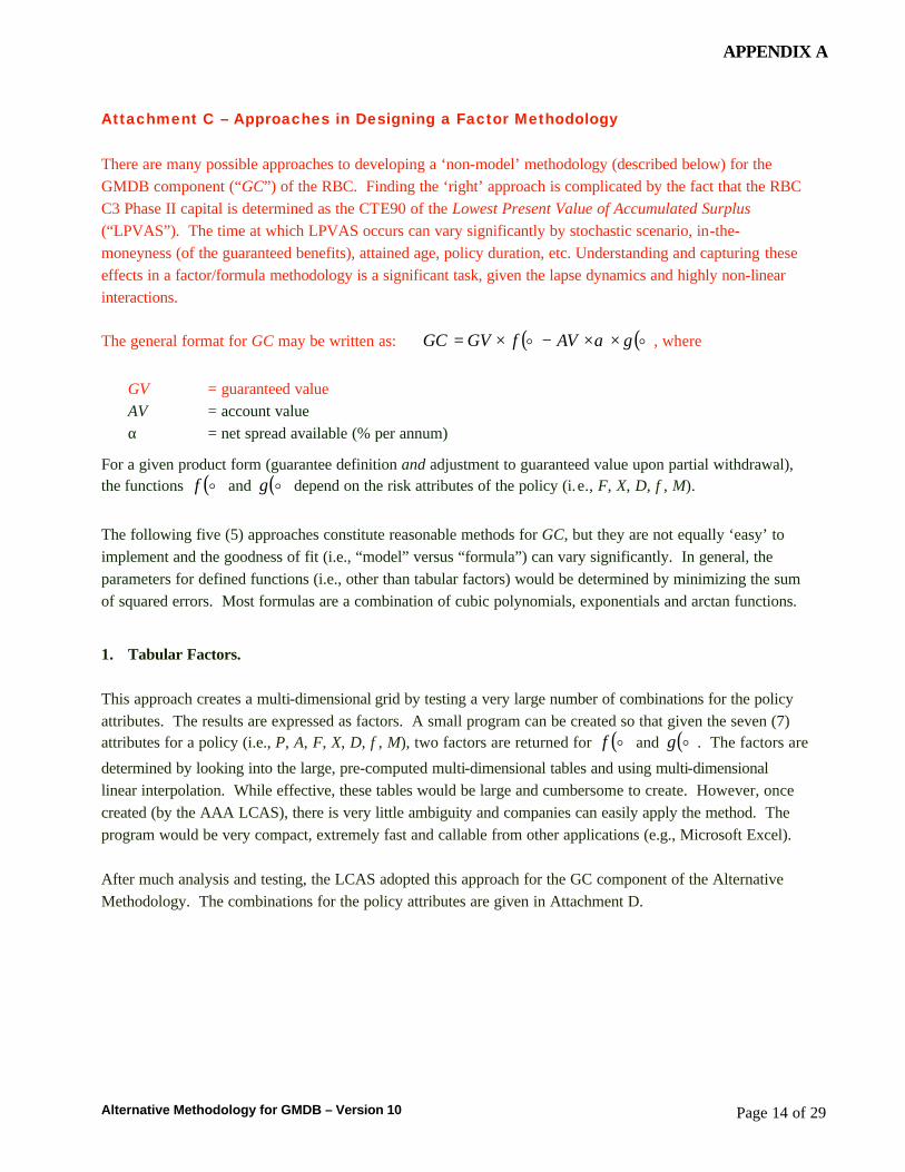
There are many possible approaches to developing a ‘non-model’ methodology (described below) for the GMDB component (“GC”) of the RBC. Finding the ‘right’ approach is complicated by the fact that the RBC C3 Phase II capital is determined as the CTE90 of the Lowest Present Value of Accumulated Surplus (“LPVAS”). The time at which LPVAS occurs can vary significantly by stochastic scenario, in-the-moneyness (of the guaranteed benefits), attained age, policy duration, etc. Understanding and capturing these effects in a factor/formula methodology is a significant task, given the lapse dynamics and highly non-linear interactions.

The general format for GC may be written as: ( ) ( )oo gAVfGVGC ××−×= α , where

GV = guaranteed value AV = account value α = net spread available (% per annum)

For a given product form (guarantee definition and adjustment to guaranteed value upon partial withdrawal), the functions ( )of and ( )og depend on the risk attributes of the policy (i.e., F, X, D, φ, M).

The following five (5) approaches constitute reasonable methods for GC, but they are not equally ‘easy’ to implement and the goodness of fit (i.e., “model” versus “formula”) can vary significantly. In general, the parameters for defined functions (i.e., other than tabular factors) would be determined by minimizing the sum of squared errors. Most formulas are a combination of cubic polynomials, exponentials and arctan functions.

1. Tabular Factors.

This approach creates a multi-dimensional grid by testing a very large number of combinations for the policy attributes. The results are expressed as factors. A small program can be created so that given the seven (7) attributes for a policy (i.e., P, A, F, X, D, φ, M), two factors are returned for ( )of and ( )og . The factors are

determined by looking into the large, pre-computed multi-dimensional tables and using multi-dimensional linear interpolation. While effective, these tables would be large and cumbersome to create. However, once created (by the AAA LCAS), there is very little ambiguity and companies can easily apply the method. The program would be very compact, extremely fast and callable from other applications (e.g., Microsoft Excel).

After much analysis and testing, the LCAS adopted this approach for the GC component of the Alternative Methodology. The combinations for the policy attributes are given in Attachment D.

APPENDIX A


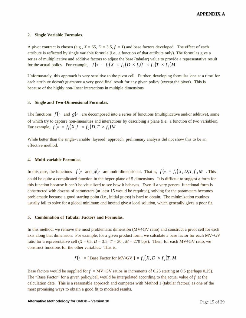
2. Single Variable Formulas.

A pivot contract is chosen (e.g., X = 65, D = 3.5, φ = 1) and base factors developed. The effect of each attribute is reflected by single variable formula (i.e., a function of that attribute only). The formulas give a series of multiplicative and additive factors to adjust the base (tabular) value to provide a representative result for the actual policy. For example, ( ) ( ) ( ) ( ) ( ) ( )MfTffDfXff 54321 ××××= φo

Unfortunately, this approach is very sensitive to the pivot cell. Further, developing formulas 'one at a time' for each attribute doesn't guarantee a very good final result for any given policy (except the pivot). This is because of the highly non-linear interactions in multiple dimensions.

3. Single and Two-Dimensional Formulas.

The functions ( )of and ( )og are decomposed into a series of functions (multiplicative and/or additive), some

of which try to capture non-linearities and interactions by describing a plane (i.e., a function of two variables). For example, ( ) ( ) ( ) ( )MfTDfXff 321 ,, ××= φo .

While better than the single-variable ‘layered’ approach, preliminary analysis did not show this to be an effective method.

4. Multi-variable Formulas.

In this case, the functions ( )of and ( )og are multi-dimensional. That is, ( ) ( )MTDXff ,,,,1 φ=o . This

could be quite a complicated function in the hyper-plane of 5 dimensions. It is difficult to suggest a form for this function because it can’t be visualized to see how it behaves. Even if a very general functional form is constructed with dozens of parameters (at least 15 would be required), solving for the parameters becomes problematic because a good starting point (i.e., initial guess) is hard to obtain. The minimization routines usually fail to solve for a global minimum and instead give a local solution, which generally gives a poor fit.

5. Combination of Tabular Factors and Formulas.

In this method, we remove the most problematic dimension (MV÷GV ratio) and construct a pivot cell for each axis along that dimension. For example, for a given product form, we calculate a base factor for each MV÷GV ratio for a representative cell (X = 65, D = 3.5, T = 30 , M = 270 bps). Then, for each MV÷GV ratio, we construct functions for the other variables. That is,

( )of = [ Base Factor for MV/GV ] ( ) ( )MTfDXf ,, 21 ××

Base factors would be supplied for φ = MV÷GV ratios in increments of 0.25 starting at 0.5 (perhaps 0.25). The “Base Factor” for a given policy/cell would be interpolated according to the actual value of φ at the calculation date. This is a reasonable approach and competes with Method 1 (tabular factors) as one of the most promising ways to obtain a good fit to modeled results.

APPENDIX A


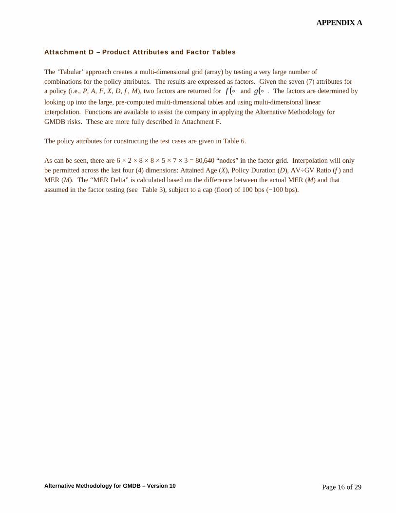
Attachment D – Product Attributes and Factor Tables The ‘Tabular’ approach creates a multi-dimensional grid (array) by testing a very large number of combinations for the policy attributes. The results are expressed as factors. Given the seven (7) attributes for a policy (i.e., P, A, F, X, D, φ, M), two factors are returned for ( )of and ( )og . The factors are determined by

looking up into the large, pre-computed multi-dimensional tables and using multi-dimensional linear interpolation. Functions are available to assist the company in applying the Alternative Methodology for GMDB risks. These are more fully described in Attachment F.

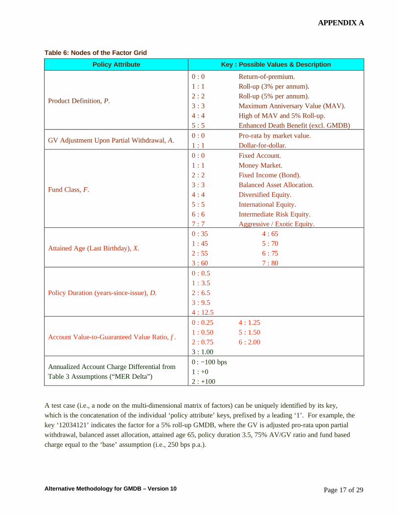
The policy attributes for constructing the test cases are given in Table 6.

As can be seen, there are 6 × 2 × 8 × 8 × 5 × 7 × 3 = 80,640 “nodes” in the factor grid. Interpolation will only be permitted across the last four (4) dimensions: Attained Age (X), Policy Duration (D), AV÷GV Ratio (φ) and MER (M). The “MER Delta” is calculated based on the difference between the actual MER (M) and that assumed in the factor testing (see Table 3), subject to a cap (floor) of 100 bps (−100 bps).

APPENDIX A


Table 6: Nodes of the Factor Grid

Policy Attribute Key : Possible Values & Description

Product Definition, P.

0 : 0 Return-of-premium. 1 : 1 Roll-up (3% per annum). 2 : 2 Roll-up (5% per annum). 3 : 3 Maximum Anniversary Value (MAV). 4 : 4 High of MAV and 5% Roll-up. 5 : 5 Enhanced Death Benefit (excl. GMDB)

GV Adjustment Upon Partial Withdrawal, A. 0 : 0 Pro-rata by market value. 1 : 1 Dollar-for-dollar.

Fund Class, F.

0 : 0 Fixed Account. 1 : 1 Money Market. 2 : 2 Fixed Income (Bond). 3 : 3 Balanced Asset Allocation. 4 : 4 Diversified Equity. 5 : 5 International Equity. 6 : 6 Intermediate Risk Equity. 7 : 7 Aggressive / Exotic Equity.

Attained Age (Last Birthday), X.

0 : 35 4 : 65 1 : 45 5 : 70 2 : 55 6 : 75 3 : 60 7 : 80

Policy Duration (years-since-issue), D.

0 : 0.5 1 : 3.5 2 : 6.5 3 : 9.5 4 : 12.5

Account Value-to-Guaranteed Value Ratio, φ.

0 : 0.25 4 : 1.25 1 : 0.50 5 : 1.50 2 : 0.75 6 : 2.00 3 : 1.00

Annualized Account Charge Differential from Table 3 Assumptions (“MER Delta”)

0 : −100 bps 1 : +0 2 : +100

A test case (i.e., a node on the multi-dimensional matrix of factors) can be uniquely identified by its key, which is the concatenation of the individual ‘policy attribute’ keys, prefixed by a leading ‘1’. For example, the key ‘12034121’ indicates the factor for a 5% roll-up GMDB, where the GV is adjusted pro-rata upon partial withdrawal, balanced asset allocation, attained age 65, policy duration 3.5, 75% AV/GV ratio and fund based charge equal to the ‘base’ assumption (i.e., 250 bps p.a.).

APPENDIX A


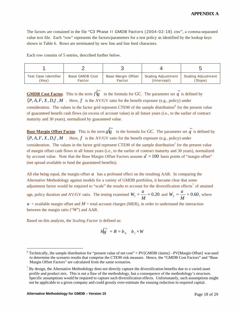
The factors are contained in the file “C3 Phase II GMDB Factors (2004-02-18).csv”, a comma-separated value text file. Each “row” represents the factors/parameters for a test policy as identified by the lookup keys shown in Table 6. Rows are terminated by new line and line feed characters.

Each row consists of 5 entries, described further below.

1 2 3 4 5 Test Case Identifier

(Key) Base GMDB Cost

Factor Base Margin Offset

Factor Scaling Adjustment

(Intercept) Scaling Adjustment

(Slope)

GMDB Cost Factor. This is the term ( )θ~

f in the formula for GC. The parameter set θ~ is defined by

( )MDXFAP ,,,,,, φ . Here, φ is the AV/GV ratio for the benefit exposure (e.g., policy) under

consideration. The values in the factor grid represent CTE90 of the sample distributionTPF

6FPT for the present value

of guaranteed benefit cash flows (in excess of account value) in all future years (i.e., to the earlier of contract maturity and 30 years), normalized by guaranteed value.

Base Margin Offset Factor. This is the term ( )θ~

g in the formula for GC. The parameter set θ~ is defined by

( )MDXFAP ,,,,,, φ . Here, φ is the AV/GV ratio for the benefit exposure (e.g., policy) under

consideration. The values in the factor grid represent CTE90 of the sample distributionP

1P for the present value

of margin offset cash flows in all future years (i.e., to the earlier of contract maturity and 30 years), normalized by account value. Note that the Base Margin Offset Factors assume 100ˆ =α basis points of “margin offset” (net spread available to fund the guaranteed benefits).

All else being equal, the margin offset α has a profound effect on the resulting AAR. In comparing the Alternative Methodology against models for a variety of GMDB portfolios, it became clear that some adjustment factor would be required to “scale” the results to account for the diversification effectsTPF

7FPT of attained

age, policy duration and AV/GV ratio. The testing examined 20.01 ==M

Wα

and 60.02 ==M

Wα

, where

α = available margin offset and M = total account charges (MER), in order to understand the interaction between the margin ratio (“W”) and AAR.

Based on this analysis, the Scaling Factor is defined as:

( ) WRh ×+== 10~ ββθ

TP

6PT Technically, the sample distribution for “present value of net cost” = PV[GMDB claims] – PV[Margin Offset] was used to determine the scenario results that comprise the CTE90 risk measure. Hence, the “GMDB Cost Factors” and “Base Margin Offset Factors” are calculated from the same scenarios.

TP

7PT By design, the Alternative Methodology does not directly capture the diversification benefits due to a varied asset profile and product mix. This is not a flaw of the methodology, but a consequence of the methodology’s structure. Specific assumptions would be required to capture such diversification effects. Unfortunately, such assumptions might not be applicable to a given company and could grossly over-estimate the ensuing reduction in required capital.

APPENDIX A


where the parameter set θ~ is defined by ( )MDXFAP ,ˆ,,,,, φ . Here, φ is the 90% of the aggregate AV/GV

for the product form (i.e., not for the individual policy or cell) under consideration. 0β and 1β are

respectively the intercept and slope for the linear relationship.

It is important to remember that ∑∑×=

GV

AV90.0φ for the product form being evaluated (e.g., all 5% Roll-up

policies). The 90% factor is meant to reflect the fact that the cost (payoff structure) for a basket of otherwise identical put options (e.g., GMDB) with varying degrees of in-the-moneyness (i.e., AV/GV ratios) is more left-skewed than the cost for a single put option at the “weighted average” asset-to-strike ratio.

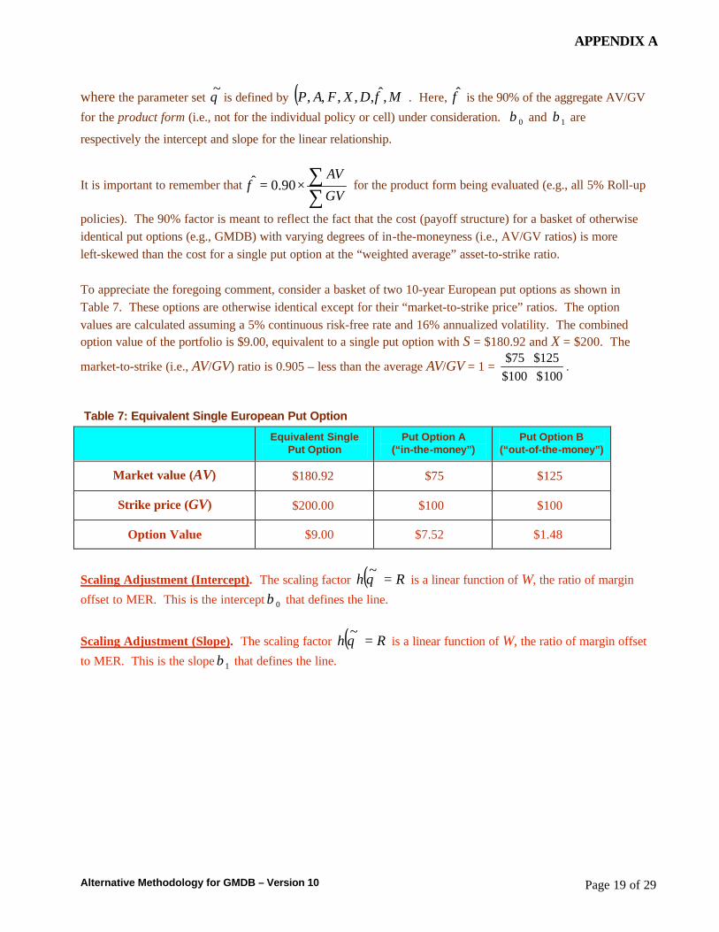
To appreciate the foregoing comment, consider a basket of two 10-year European put options as shown in Table 7. These options are otherwise identical except for their “market-to-strike price” ratios. The option values are calculated assuming a 5% continuous risk-free rate and 16% annualized volatility. The combined option value of the portfolio is $9.00, equivalent to a single put option with S = $180.92 and X = $200. The

market-to-strike (i.e., AV/GV) ratio is 0.905 – less than the average AV/GV = 1 = 100$100$

125$75$+

+.

Table 7: Equivalent Single European Put Option

Equivalent Single

Put Option Put Option A

(“in-the-money”) Put Option B

(“out-of-the-money”)

Market value (AV) $180.92 $75 $125

Strike price (GV) $200.00 $100 $100

Option Value $9.00 $7.52 $1.48

Scaling Adjustment (Intercept). The scaling factor ( ) Rh =θ~

is a linear function of W, the ratio of margin

offset to MER. This is the intercept 0β that defines the line.

Scaling Adjustment (Slope). The scaling factor ( ) Rh =θ~

is a linear function of W, the ratio of margin offset

to MER. This is the slope 1β that defines the line.

APPENDIX A


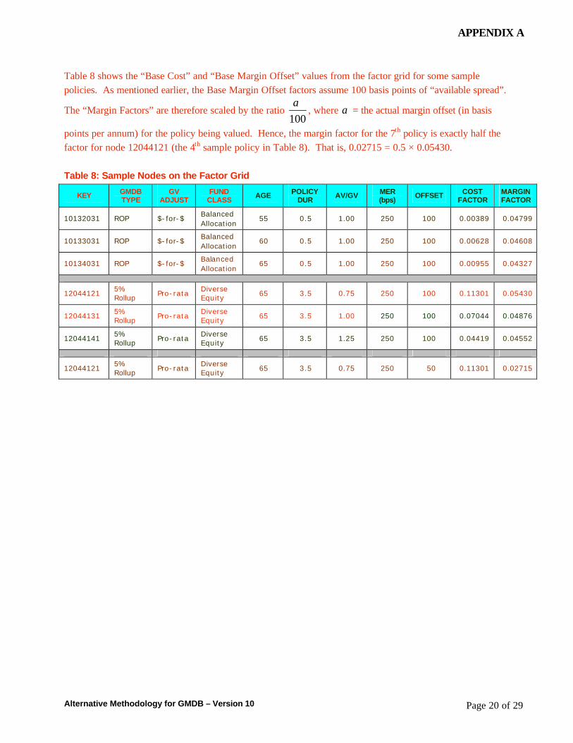
Table 8 shows the “Base Cost” and “Base Margin Offset” values from the factor grid for some sample policies. As mentioned earlier, the Base Margin Offset factors assume 100 basis points of “available spread”.

The “Margin Factors” are therefore scaled by the ratio 100α

, where α = the actual margin offset (in basis

points per annum) for the policy being valued. Hence, the margin factor for the 7P

thP policy is exactly half the

factor for node 12044121 (the 4P

thP sample policy in Table 8). That is, 0.02715 = 0.5 × 0.05430.

Table 8: Sample Nodes on the Factor Grid

KEY GMDB TYPE

GV ADJUST

FUND CLASS

AGE POLICY DUR

AV/GV MER (bps)

OFFSET COST FACTOR

MARGIN FACTOR

10132031 ROP $-for-$ Balanced Allocation

55 0.5 1.00 250 100 0.00389 0.04799


60 0.5 1.00 250 100 0.00628 0.04608


65 0.5 1.00 250 100 0.00955 0.04327

12044121 5% Rollup

Pro-rata Diverse Equity

65 3.5 0.75 250 100 0.11301 0.05430

12044131 5% Rollup


65 3.5 1.00 250 100 0.07044 0.04876

12044141 5% Rollup


65 3.5 1.25 250 100 0.04419 0.04552

12044121 5% Rollup


65 3.5 0.75 250 50 0.11301 0.02715

APPENDIX A


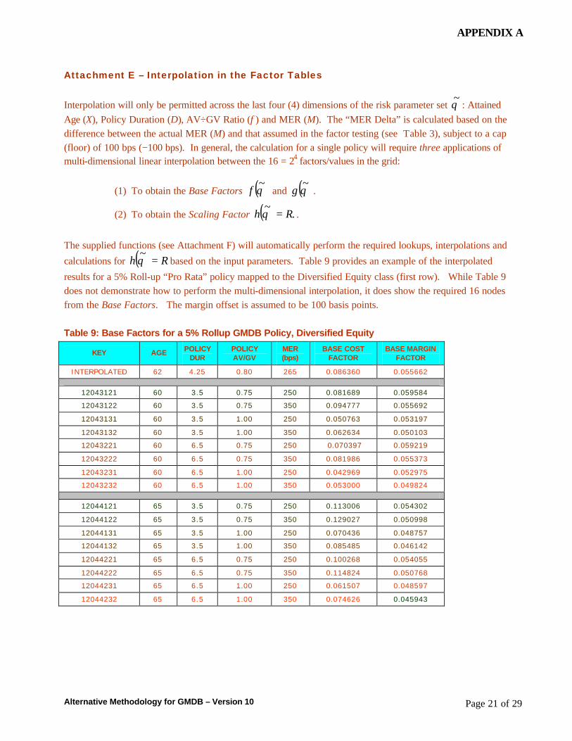
Attachment E – Interpolation in the Factor Tables Interpolation will only be permitted across the last four (4) dimensions of the risk parameter set θ~ : Attained Age (X), Policy Duration (D), AV÷GV Ratio (φ) and MER (M). The “MER Delta” is calculated based on the difference between the actual MER (M) and that assumed in the factor testing (see Table 3), subject to a cap (floor) of 100 bps (−100 bps). In general, the calculation for a single policy will require three applications of multi-dimensional linear interpolation between the 16 = 2P

4P factors/values in the grid:

(1) To obtain the Base Factors ( )θ~

f and ( )θ~

g .

(2) To obtain the Scaling Factor ( ) .~

Rh =θ .

The supplied functions (see Attachment F) will automatically perform the required lookups, interpolations and

calculations for ( ) Rh =θ~

based on the input parameters. Table 9 provides an example of the interpolated

results for a 5% Roll-up “Pro Rata” policy mapped to the Diversified Equity class (first row). While Table 9 does not demonstrate how to perform the multi-dimensional interpolation, it does show the required 16 nodes from the Base Factors. The margin offset is assumed to be 100 basis points.

Table 9: Base Factors for a 5% Rollup GMDB Policy, Diversified Equity

KEY AGE POLICY DUR

POLICY AV/GV

MER (bps)

BASE COST FACTOR

BASE MARGIN FACTOR

INTERPOLATED 62 4.25 0.80 265 0.086360 0.055662

12043121 60 3.5 0.75 250 0.081689 0.059584

12043122 60 3.5 0.75 350 0.094777 0.055692

12043131 60 3.5 1.00 250 0.050763 0.053197

12043132 60 3.5 1.00 350 0.062634 0.050103

12043221 60 6.5 0.75 250 0.070397 0.059219

12043222 60 6.5 0.75 350 0.081986 0.055373

12043231 60 6.5 1.00 250 0.042969 0.052975

12043232 60 6.5 1.00 350 0.053000 0.049824

12044121 65 3.5 0.75 250 0.113006 0.054302

12044122 65 3.5 0.75 350 0.129027 0.050998

12044131 65 3.5 1.00 250 0.070436 0.048757

12044132 65 3.5 1.00 350 0.085485 0.046142

12044221 65 6.5 0.75 250 0.100268 0.054055

12044222 65 6.5 0.75 350 0.114824 0.050768

12044231 65 6.5 1.00 250 0.061507 0.048597

12044232 65 6.5 1.00 350 0.074626 0.045943

APPENDIX A


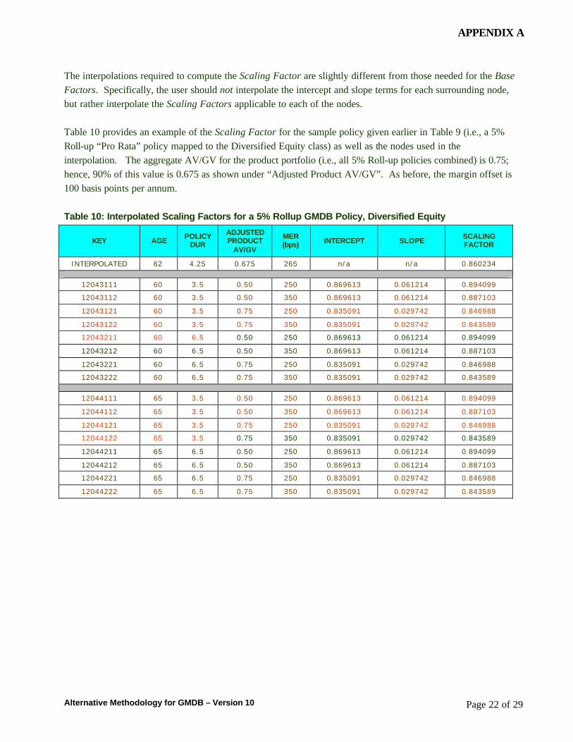
The interpolations required to compute the Scaling Factor are slightly different from those needed for the Base Factors. Specifically, the user should not interpolate the intercept and slope terms for each surrounding node, but rather interpolate the Scaling Factors applicable to each of the nodes.

Table 10 provides an example of the Scaling Factor for the sample policy given earlier in Table 9 (i.e., a 5% Roll-up “Pro Rata” policy mapped to the Diversified Equity class) as well as the nodes used in the interpolation. The aggregate AV/GV for the product portfolio (i.e., all 5% Roll-up policies combined) is 0.75; hence, 90% of this value is 0.675 as shown under “Adjusted Product AV/GV”. As before, the margin offset is 100 basis points per annum.

Table 10: Interpolated Scaling Factors for a 5% Rollup GMDB Policy, Diversified Equity

KEY AGE POLICY

DUR

ADJUSTED PRODUCT

AV/GV

MER (bps) INTERCEPT SLOPE

SCALING FACTOR

INTERPOLATED 62 4.25 0.675 265 n/a n/a 0.860234

12043111 60 3.5 0.50 250 0.869613 0.061214 0.894099

12043112 60 3.5 0.50 350 0.869613 0.061214 0.887103

12043121 60 3.5 0.75 250 0.835091 0.029742 0.846988

12043122 60 3.5 0.75 350 0.835091 0.029742 0.843589

12043211 60 6.5 0.50 250 0.869613 0.061214 0.894099

12043212 60 6.5 0.50 350 0.869613 0.061214 0.887103

12043221 60 6.5 0.75 250 0.835091 0.029742 0.846988

12043222 60 6.5 0.75 350 0.835091 0.029742 0.843589

12044111 65 3.5 0.50 250 0.869613 0.061214 0.894099

12044112 65 3.5 0.50 350 0.869613 0.061214 0.887103

12044121 65 3.5 0.75 250 0.835091 0.029742 0.846988

12044122 65 3.5 0.75 350 0.835091 0.029742 0.843589

12044211 65 6.5 0.50 250 0.869613 0.061214 0.894099

12044212 65 6.5 0.50 350 0.869613 0.061214 0.887103

12044221 65 6.5 0.75 250 0.835091 0.029742 0.846988

12044222 65 6.5 0.75 350 0.835091 0.029742 0.843589

APPENDIX A


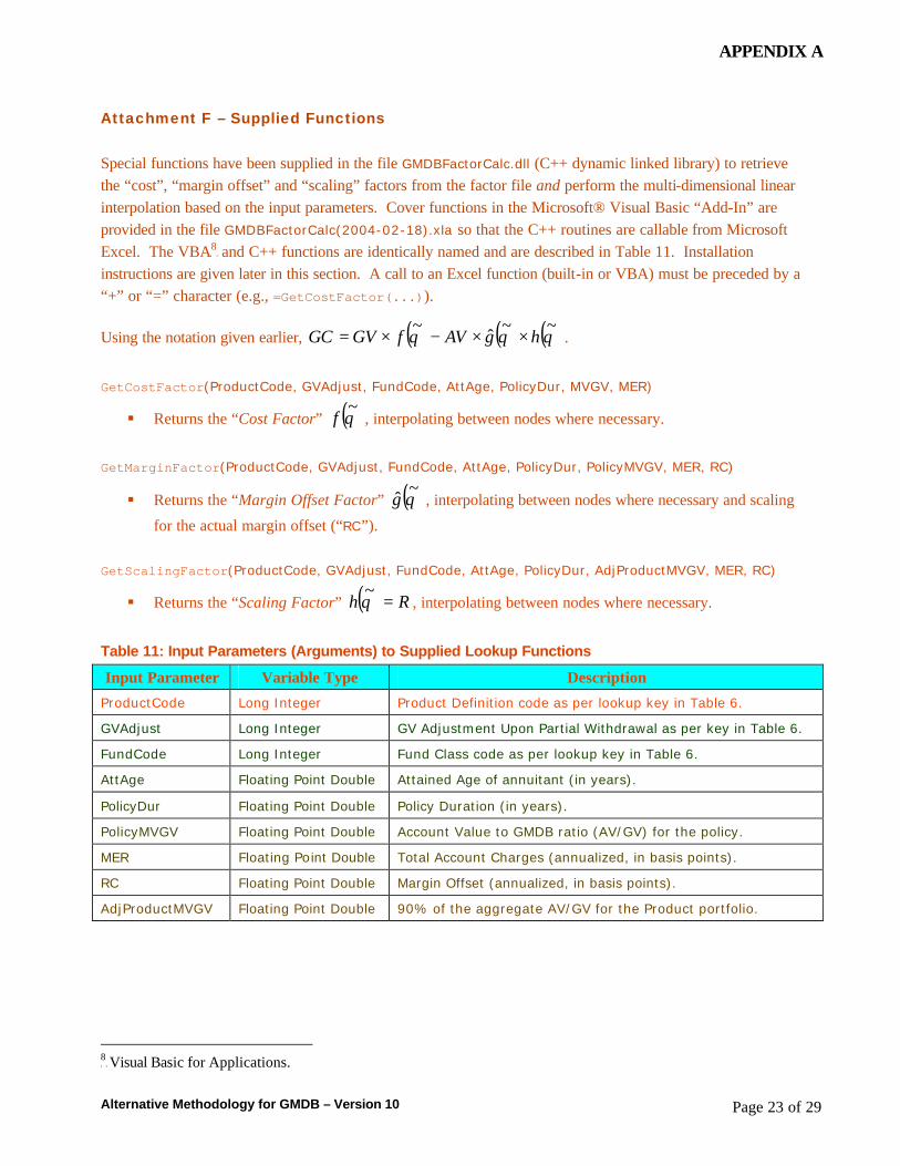
Attachment F – Supplied Functions Special functions have been supplied in the file GMDBFactorCalc.dll (C++ dynamic linked library) to retrieve the “cost”, “margin offset” and “scaling” factors from the factor file and perform the multi-dimensional linear interpolation based on the input parameters. Cover functions in the Microsoft® Visual Basic “Add-In” are provided in the file GMDBFactorCalc(2004-02-18).xla so that the C++ routines are callable from Microsoft Excel. The VBATPF

8FPT and C++ functions are identically named and are described in Table 11. Installation

instructions are given later in this section. A call to an Excel function (built-in or VBA) must be preceded by a “+” or “=” character (e.g., =GetCostFactor(...)).

Using the notation given earlier, ( ) ( ) ( )θθθ~~ˆ~

hgAVfGVGC ××−×= .

GetCostFactor(ProductCode, GVAdjust, FundCode, AttAge, PolicyDur, MVGV, MER)

§ Returns the “Cost Factor” ( )θ~

f , interpolating between nodes where necessary.

GetMarginFactor(ProductCode, GVAdjust, FundCode, AttAge, PolicyDur, PolicyMVGV, MER, RC)

§ Returns the “Margin Offset Factor” ( )θ~

g , interpolating between nodes where necessary and scaling

for the actual margin offset (“RC”).

GetScalingFactor(ProductCode, GVAdjust, FundCode, AttAge, PolicyDur, AdjProductMVGV, MER, RC)

§ Returns the “Scaling Factor” ( ) Rh =θ~

, interpolating between nodes where necessary.

Table 11: Input Parameters (Arguments) to Supplied Lookup Functions

Input Parameter Variable Type Description

ProductCode Long Integer Product Definition code as per lookup key in Table 6.

GVAdjust Long Integer GV Adjustment Upon Partial Withdrawal as per key in Table 6.

FundCode Long Integer Fund Class code as per lookup key in Table 6.

AttAge Floating Point Double Attained Age of annuitant (in years).

PolicyDur Floating Point Double Policy Duration (in years).

PolicyMVGV Floating Point Double Account Value to GMDB ratio (AV/GV) for the policy.

MER Floating Point Double Total Account Charges (annualized, in basis points).

RC Floating Point Double Margin Offset (annualized, in basis points).

AdjProductMVGV Floating Point Double 90% of the aggregate AV/GV for the Product portfolio.

TP

8PT Visual Basic for Applications.

APPENDIX A


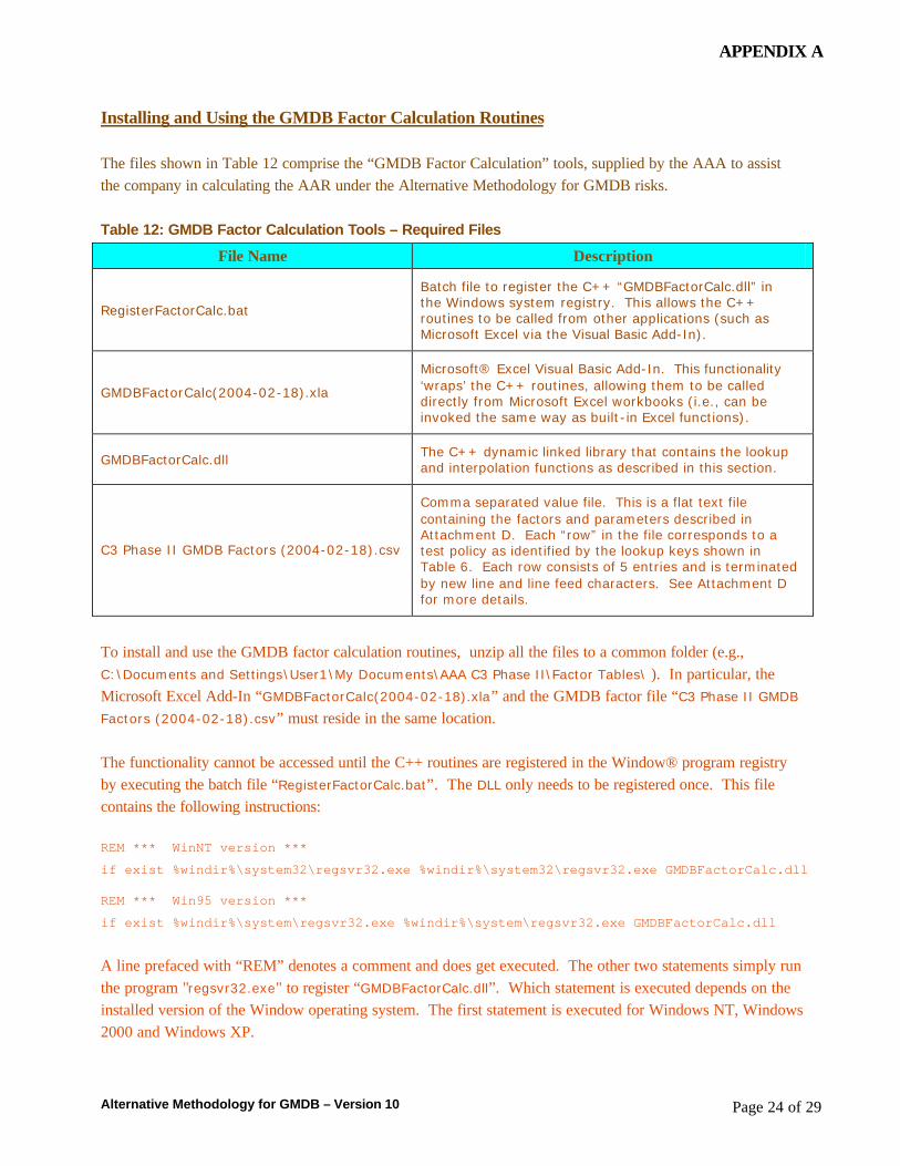
Installing and Using the GMDB Factor Calculation Routines

The files shown in Table 12 comprise the “GMDB Factor Calculation” tools, supplied by the AAA to assist the company in calculating the AAR under the Alternative Methodology for GMDB risks.

Table 12: GMDB Factor Calculation Tools – Required Files

File Name Description

RegisterFactorCalc.bat

Batch file to register the C++ “GMDBFactorCalc.dll” in the Windows system registry. This allows the C++ routines to be called from other applications (such as Microsoft Excel via the Visual Basic Add-In).

GMDBFactorCalc(2004-02-18).xla

Microsoft® Excel Visual Basic Add-In. This functionality ‘wraps’ the C++ routines, allowing them to be called directly from Microsoft Excel workbooks (i.e., can be invoked the same way as built-in Excel functions).

GMDBFactorCalc.dll The C++ dynamic linked library that contains the lookup and interpolation functions as described in this section.

C3 Phase II GMDB Factors (2004-02-18).csv

Comma separated value file. This is a flat text file containing the factors and parameters described in Attachment D. Each “row” in the file corresponds to a test policy as identified by the lookup keys shown in Table 6. Each row consists of 5 entries and is terminated by new line and line feed characters. See Attachment D for more details.

To install and use the GMDB factor calculation routines, unzip all the files to a common folder (e.g., C:\Documents and Settings\User1\My Documents\AAA C3 Phase II\Factor Tables\ ). In particular, the Microsoft Excel Add-In “GMDBFactorCalc(2004-02-18).xla” and the GMDB factor file “C3 Phase II GMDB

Factors (2004-02-18).csv” must reside in the same location.

The functionality cannot be accessed until the C++ routines are registered in the Window® program registry by executing the batch file “RegisterFactorCalc.bat”. The DLL only needs to be registered once. This file contains the following instructions:

REM *** WinNT version ***

if exist %windir%\system32\regsvr32.exe %windir%\system32\regsvr32.exe GMDBFactorCalc.dll

REM *** Win95 version ***

if exist %windir%\system\regsvr32.exe %windir%\system\regsvr32.exe GMDBFactorCalc.dll

A line prefaced with “REM” denotes a comment and does get executed. The other two statements simply run the program "regsvr32.exe" to register “GMDBFactorCalc.dll”. Which statement is executed depends on the installed version of the Window operating system. The first statement is executed for Windows NT, Windows 2000 and Windows XP.

APPENDIX A


If "regsvr32.exe" does not exist in the Windows system directory, then the “GMDBFactorCalc.dll” does not get entered into the registry. In this case, use the Windows Explorer to locate "regsvr32.exe" on your local drive(s). Suppose it exists in the folder c:\Windows System Folder\. Then edit RegisterFactorCalc.bat, remove all the existing lines and then type c:\Windows System Folder\regsvr32.exe GMDBFactorCalc.dll Save the file, exit and execute (run).

When the C++ DLL is successfully registered, you should receive a message such as the following:

The Microsoft Add-In must be loaded (into Excel) before the VBA functions can be called. Remember that the factor file and the Microsoft Excel Add-In (*.xla) should reside in the same folder. Simply open “GMDBFactorCalc(2004-02-18).xla” from Microsoft Excel. To view the VBA program, press [Alt-F11].

Under the VBAProject (GMDBFactorCalc(2004-02-18).xla) there are two important items. First, there is a module named “FactorCalc”. This module contains the VBA cover functions for calling the C++ factor engine and some initialization parameters. The only line of code that may need editing is:

Public Const FactorFile As String = "C3 Phase II GMDB Factors (2004-02-18).csv"

This statement defines the variable FactorFile as a character vector (string) and assigns the name of the factor file (without the directory). If the factor file is renamed, the user must edit the string (encased in double quotes), provided the correct name and save the .xla. Do not remove or change the .csv extension.

Second, there is a Microsoft Excel Object entitled “This Workbook”. This is a special object that exists in all Excel workbooks. The VBA code in this object initializes the factor calculation engine and loads the factor file into memory for faster execution by the statement:

Call m_FactorEngine.LoadFactorFile(ThisWorkbook.Path + "\" + FactorFile)

Here we clearly see that the factor file is assumed to reside in the same folder (“path”) as “ThisWorkbook” (i.e., GMDBFactorCalc(2004-02-18).xla).

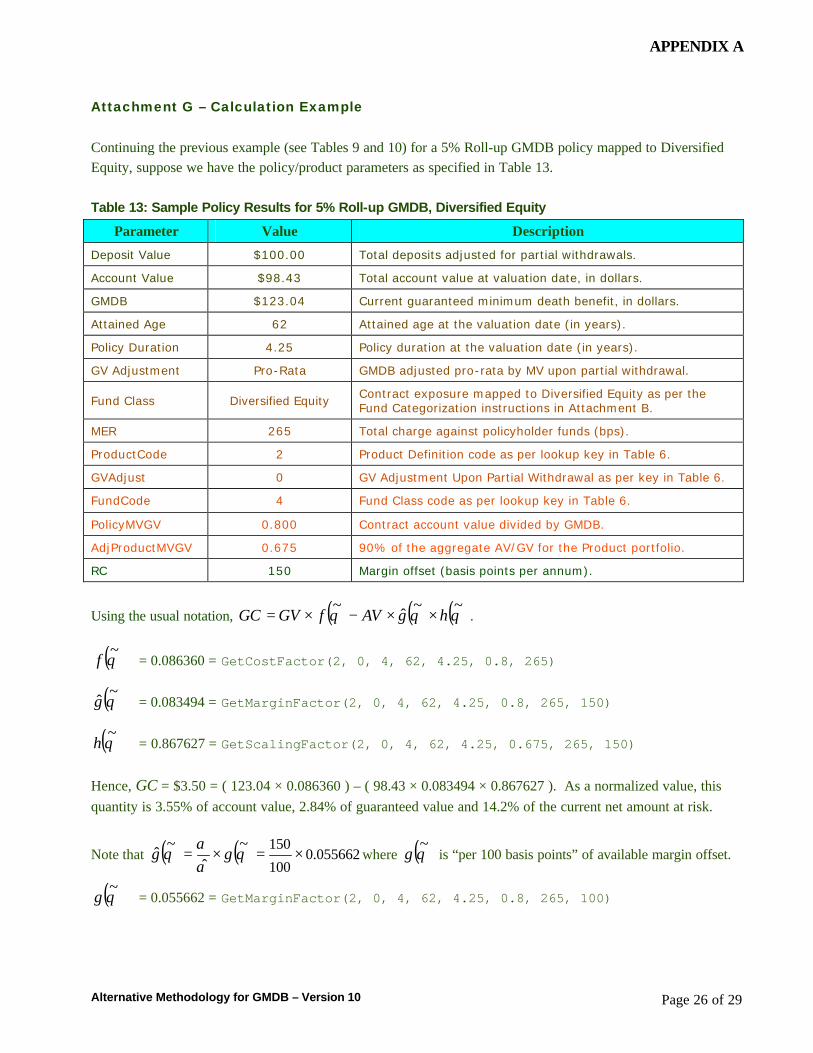
APPENDIX A


Attachment G – Calculation Example

Continuing the previous example (see Tables 9 and 10) for a 5% Roll-up GMDB policy mapped to Diversified Equity, suppose we have the policy/product parameters as specified in Table 13.

Table 13: Sample Policy Results for 5% Roll-up GMDB, Diversified Equity

Parameter Value Description

Deposit Value $100.00 Total deposits adjusted for partial withdrawals.

Account Value $98.43 Total account value at valuation date, in dollars.

GMDB $123.04 Current guaranteed minimum death benefit, in dollars.

Attained Age 62 Attained age at the valuation date (in years).

Policy Duration 4.25 Policy duration at the valuation date (in years).

GV Adjustment Pro-Rata GMDB adjusted pro-rata by MV upon partial withdrawal.

Fund Class Diversified Equity Contract exposure mapped to Diversified Equity as per the Fund Categorization instructions in Attachment B.

MER 265 Total charge against policyholder funds (bps).

ProductCode 2 Product Definition code as per lookup key in Table 6.

GVAdjust 0 GV Adjustment Upon Partial Withdrawal as per key in Table 6.

FundCode 4 Fund Class code as per lookup key in Table 6.

PolicyMVGV 0.800 Contract account value divided by GMDB.

AdjProductMVGV 0.675 90% of the aggregate AV/GV for the Product portfolio.

RC 150 Margin offset (basis points per annum).

Using the usual notation, ( ) ( ) ( )θθθ

~~ˆ~hgAVfGVGC ××−×= .

( )θ~

f = 0.086360 = GetCostFactor(2, 0, 4, 62, 4.25, 0.8, 265)

( )θ~

g = 0.083494 = GetMarginFactor(2, 0, 4, 62, 4.25, 0.8, 265, 150)

( )θ~

h = 0.867627 = GetScalingFactor(2, 0, 4, 62, 4.25, 0.675, 265, 150)

Hence, GC = $3.50 = ( 123.04 × 0.086360 ) – ( 98.43 × 0.083494 × 0.867627 ). As a normalized value, this quantity is 3.55% of account value, 2.84% of guaranteed value and 14.2% of the current net amount at risk.

Note that ( ) ( ) 0.055662100

150~ˆ

~ˆ ×=×= θαα

θ gg where ( )θ~

g is “per 100 basis points” of available margin offset.

( )θ~

g = 0.055662 = GetMarginFactor(2, 0, 4, 62, 4.25, 0.8, 265, 100)

APPENDIX A


Attachment H – Derivation of Account Charges (MER) and Margin Offset (α) The total account charge (“MER”) is meant to capture all amounts that are deducted from policyholder funds, not only those that are commonly expressed as spread-based fees. The MER, expressed as an equivalent annual basis point charge against account value, should include (but not be limited to) the following: investment management fees, mortality & expense charges, administrative loads, policy fees and risk premiums. In light of the foregoing, it may be necessary to estimate the “equivalent MER” if there are fees withdrawn from policyholder accounts that are not expressed as basis point charges against account value.

The margin offset represents the total amount available to fund the guaranteed benefits, after considering all other policy expenses (including overhead). The margin offset, expressed as an equivalent annual basis point charge against account value, should be deemed “permanently available” in all future scenarios. However, the margin offset should not include per policy charges (e.g., annual policy fees) since these are included in FE.

APPENDIX A


Attachment I – Adjustments to GC for Product Variations & Risk Mitigation/Transfer

In some cases, it may be necessary for the company to make adjustments to the published factors due to:

1. A variation in product form wherein the definition of the guaranteed benefit is materially different from those for which factors are available (see Table 2 in Attachment A); and/or

2. A risk mitigation / management strategy that cannot be accommodated through a straight-forward and direct adjustment to the published values.

Any adjustments to the published factors must be fully documented and supported through stochastic analysis. Such analysis may require stochastic simulations, but would not ordinarily be based on full inforce projections. Instead, a representative “model office” should be sufficient. In the absence of material changes to the product design, risk management program and Alternative Methodology (including the published factors), the company would not be expected to redo this analysis each year.

Note that minor variations in product design do not necessarily require additional effort. In some cases, it may be reasonable to use the factors/formulas for a different product form (e.g., for a “roll-up” GMDB policy near or beyond the maximum reset age or amount, the company should use the “return-of-premium” GMDB factors/formulas, possibly adjusting the guaranteed value to reflect further resets, if any). In other cases, the company might determine the RBC based on two different guarantee definitions and interpolate the results to obtain an appropriate value for the given policy/cell. Likewise, it may be possible to adjust the Alternative Methodology results for certain risk transfer arrangements without significant additional work (e.g., quota-share reinsurance without caps, floors or sliding scales would normally be reflected by a simple pro-rata adjustment to the “gross” GC results).

However, if the policy design is sufficiently different from those provided and/or the risk mitigation strategy is non-linear (e.g., hedging) in its impact on the AAR, and there is no practical or obvious way to obtain a good result from the prescribed factors/formulas, the company must justify any adjustments or approximations by stochastic modeling. Notably this modeling need not be performed on the whole portfolio, but can be undertaken on an appropriate set of representative policies.

The remainder of this Attachment suggests a process for adjusting the published “Cost” and “Margin Offset” factors due to a variation in product design (e.g., a “step-up” option at every 7P

thP anniversary whereby the

guaranteed value is reset to the account value, if higher). Note that the “Scaling Factors” (as determined by the slope and intercept terms in the factor table) would not be adjusted.

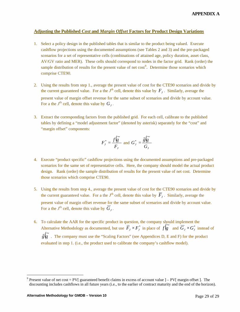
APPENDIX A


Adjusting the Published Cost and Margin Offset Factors for Product Design Variations

1. Select a policy design in the published tables that is similar to the product being valued. Execute cashflow projections using the documented assumptions (see Tables 2 and 3) and the pre-packaged scenarios for a set of representative cells (combinations of attained age, policy duration, asset class, AV/GV ratio and MER). These cells should correspond to nodes in the factor grid. Rank (order) the sample distribution of results for the present value of net costTPF

9FPT. Determine those scenarios which

comprise CTE90.

2. Using the results from step 1., average the present value of cost for the CTE90 scenarios and divide by the current guaranteed value. For a the J P

thP cell, denote this value by JF . Similarly, average the

present value of margin offset revenue for the same subset of scenarios and divide by account value. For a the J P

thP cell, denote this value by JG .

3. Extract the corresponding factors from the published grid. For each cell, calibrate to the published tables by defining a “model adjustment factor” (denoted by asterisk) separately for the “cost” and “margin offset” components:

( )J

J Ff

Fθ~* = and

( )J

J Gg

Gθ~ˆ* =

4. Execute “product specific” cashflow projections using the documented assumptions and pre-packaged scenarios for the same set of representative cells. Here, the company should model the actual product design. Rank (order) the sample distribution of results for the present value of net cost. Determine those scenarios which comprise CTE90.

5. Using the results from step 4., average the present value of cost for the CTE90 scenarios and divide by the current guaranteed value. For a the J P

thP cell, denote this value by JF . Similarly, average the

present value of margin offset revenue for the same subset of scenarios and divide by account value. For a the J P

thP cell, denote this value by JG .

6. To calculate the AAR for the specific product in question, the company should implement the Alternative Methodology as documented, but use *

JJ FF × in place of ( )θ~

f and *JJ GG × instead of

( )θ~

g . The company must use the “Scaling Factors” (see Appendices D, E and F) for the product

evaluated in step 1. (i.e., the product used to calibrate the company’s cashflow model).

TP

9PT Present value of net cost = PV[ guaranteed benefit claims in excess of account value ] – PV[ margin offset ]. The discounting includes cashflows in all future years (i.e., to the earlier of contract maturity and the end of the horizon).

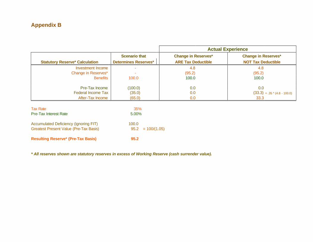
Appendix B

Actual Experience Scenario that Change in Reserves* Change in Reserves* Statutory Reserve* Calculation Determines Reserves* ARE Tax Deductible NOT Tax Deductible Investment Income - 4.8 4.8 Change in Reserves* - (95.2) (95.2) Benefits 100.0 100.0 100.0 Pre-Tax Income (100.0) 0.0 0.0 Federal Income Tax (35.0) 0.0 (33.3) = .35 * (4.8 - 100.0)

After-Tax Income (65.0) 0.0 33.3 Tax Rate 35% Pre-Tax Interest Rate 5.00% Accumulated Deficiency (ignoring FIT) 100.0 Greatest Present Value (Pre-Tax Basis) 95.2 = 100/(1.05) Resulting Reserve* (Pre-Tax Basis) 95.2 * All reserves shown are statutory reserves in excess of Working Reserve (cash surrender value).

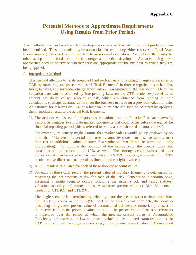
Appendix C

1

Potential Methods to Approximate Requirements Using Results from Prior Periods

Two methods that can be a basis for meeting the criteria established in the draft guideline have been identified. These methods may be appropriate for estimating either reserves or Total Asset Requirements (TAR) and are offered for discussion and evaluation. We believe there may be other acceptable methods that could emerge as practice develops. Actuaries using these approaches need to determine whether they are appropriate for the business to which they are being applied.

A. Interpolation Method

This method attempts to relate projected fund performance to resulting changes in reserves or TAR by measuring the present values of "Risk Elements" in three categories: death benefits, living benefits, and surrender charge amortization. An estimate of the reserve or TAR on the valuation date can be obtained by interpolating between the CTE results, expressed as an amount per dollar of net amount at risk, which are obtained from running multiple calculations (perhaps as many as five) on the business in force on a previous valuation date. An estimate for reserves or TAR at a later valuation date can then be obtained by applying the interpolated result to the actual Risk Elements.

1) The account values as of the previous valuation date are “shocked” up and down by various percentages to simulate market movements that could occur before the end of the financial reporting period (this is referred to below as the "shocked account values").

For example, an actuary might assume that market values would go up or down by no more than 15% over this period (if markets change by more than this, the actuary must then run an additional valuation since “extrapolation” would not be permitted – only interpolation). To improve the accuracy of the interpolation, the actuary might also choose to run projections at +/- 10%, as well. The starting account values and asset values would then be increased by +/- 10% and +/- 15%, resulting in calculation of CTE results on five different starting values (including the original values).

2) A CTE result is calculated for each of these shocked account values.

3) For each of these CTE results, the present value of the Risk Elements is determined by measuring the net amounts at risk for each of the Risk Elements on a seriatim basis, assuming a single scenario occurs following the initial shock and using statutory valuation mortality and interest rates. A separate present value of Risk Elements is needed for CTE (65) and CTE (90).

The single scenario is determined by selecting, from the scenarios run to determine either the CTE (65) reserve or the CTE (90) TAR on the previous valuation date, the scenario producing the greatest present value of accumulated deficiencies numerically closest to the reserve held on the previous valuation date. The present value of the Risk Elements is measured over the period at which the greatest present value of Accumulated Deficiency for reserves, or lowest present value of accumulated statutory surplus for TAR, occurs within the single scenario (e.g., if the greatest present value of Accumulated

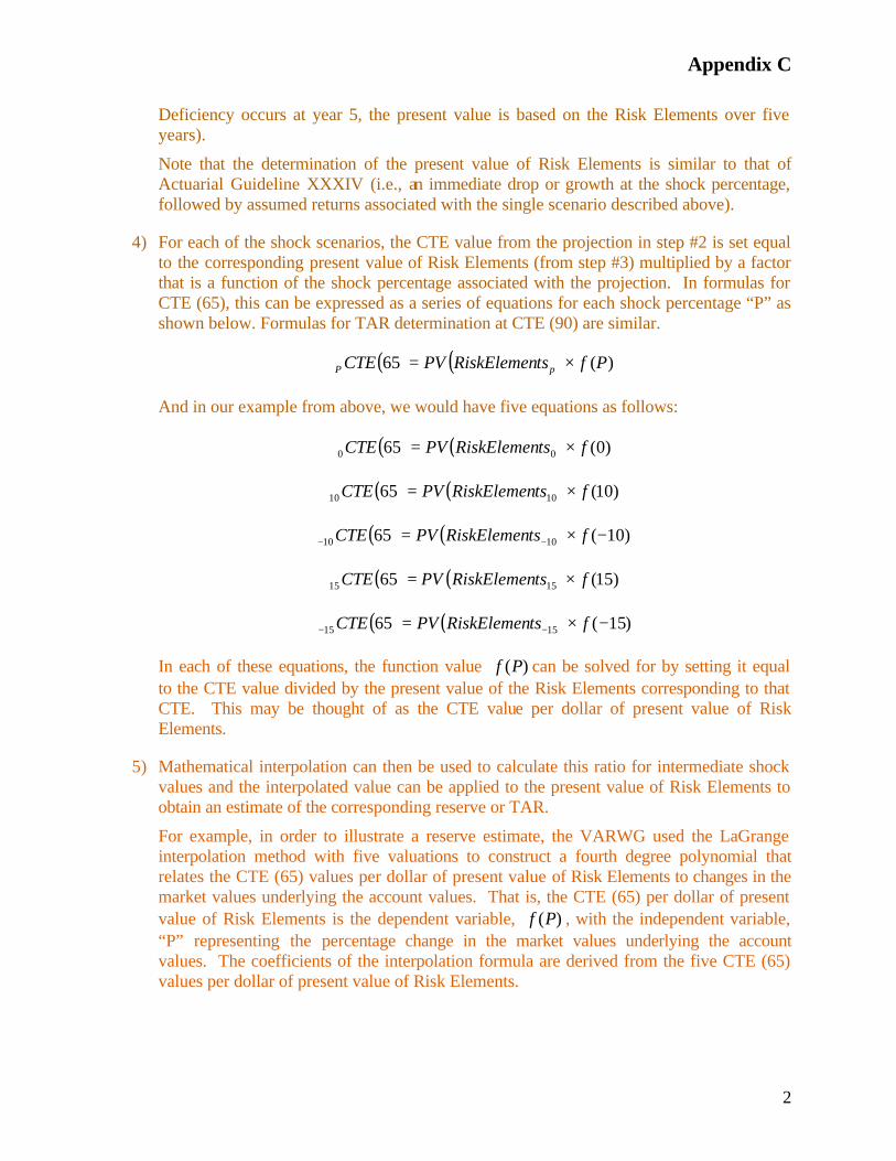
Appendix C

2

Deficiency occurs at year 5, the present value is based on the Risk Elements over five years).

Note that the determination of the present value of Risk Elements is similar to that of Actuarial Guideline XXXIV (i.e., an immediate drop or growth at the shock percentage, followed by assumed returns associated with the single scenario described above).

4) For each of the shock scenarios, the CTE value from the projection in step #2 is set equal to the corresponding present value of Risk Elements (from step #3) multiplied by a factor that is a function of the shock percentage associated with the projection. In formulas for CTE (65), this can be expressed as a series of equations for each shock percentage “P” as shown below. Formulas for TAR determination at CTE (90) are similar.

( ) ( ) )(65 PftsRiskElemenPVCTE pP ×=

And in our example from above, we would have five equations as follows:

( ) ( ) )0(65 00 ftsRiskElemenPVCTE ×=


( ) ( ) )10(65 1010 −×= −− ftsRiskElemenPVCTE


( ) ( ) )15(65 1515 −×= −− ftsRiskElemenPVCTE

In each of these equations, the function value )(Pf can be solved for by setting it equal to the CTE value divided by the present value of the Risk Elements corresponding to that CTE. This may be thought of as the CTE value per dollar of present value of Risk Elements.

5) Mathematical interpolation can then be used to calculate this ratio for intermediate shock values and the interpolated value can be applied to the present value of Risk Elements to obtain an estimate of the corresponding reserve or TAR.

For example, in order to illustrate a reserve estimate, the VARWG used the LaGrange interpolation method with five valuations to construct a fourth degree polynomial that relates the CTE (65) values per dollar of present value of Risk Elements to changes in the market values underlying the account values. That is, the CTE (65) per dollar of present value of Risk Elements is the dependent variable, )(Pf , with the independent variable, “P” representing the percentage change in the market values underlying the account values. The coefficients of the interpolation formula are derived from the five CTE (65) values per dollar of present value of Risk Elements.

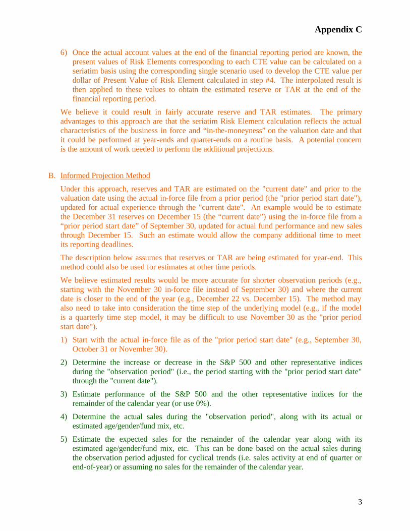
Appendix C

3

6) Once the actual account values at the end of the financial reporting period are known, the present values of Risk Elements corresponding to each CTE value can be calculated on a seriatim basis using the corresponding single scenario used to develop the CTE value per dollar of Present Value of Risk Element calculated in step #4. The interpolated result is then applied to these values to obtain the estimated reserve or TAR at the end of the financial reporting period.

We believe it could result in fairly accurate reserve and TAR estimates. The primary advantages to this approach are that the seriatim Risk Element calculation reflects the actual characteristics of the business in force and “in-the-moneyness” on the valuation date and that it could be performed at year-ends and quarter-ends on a routine basis. A potential concern is the amount of work needed to perform the additional projections.

B. Informed Projection Method

Under this approach, reserves and TAR are estimated on the "current date" and prior to the valuation date using the actual in-force file from a prior period (the "prior period start date"), updated for actual experience through the "current date". An example would be to estimate the December 31 reserves on December 15 (the “current date”) using the in-force file from a “prior period start date” of September 30, updated for actual fund performance and new sales through December 15. Such an estimate would allow the company additional time to meet its reporting deadlines.

The description below assumes that reserves or TAR are being estimated for year-end. This method could also be used for estimates at other time periods.

We believe estimated results would be more accurate for shorter observation periods (e.g., starting with the November 30 in-force file instead of September 30) and where the current date is closer to the end of the year (e.g., December 22 vs. December 15). The method may also need to take into consideration the time step of the underlying model (e.g., if the model is a quarterly time step model, it may be difficult to use November 30 as the "prior period start date").

1) Start with the actual in-force file as of the "prior period start date" (e.g., September 30, October 31 or November 30).

2) Determine the increase or decrease in the S&P 500 and other representative indices during the "observation period" (i.e., the period starting with the "prior period start date" through the "current date").

3) Estimate performance of the S&P 500 and the other representative indices for the remainder of the calendar year (or use 0%).

4) Determine the actual sales during the "observation period", along with its actual or estimated age/gender/fund mix, etc.

5) Estimate the expected sales for the remainder of the calendar year along with its estimated age/gender/fund mix, etc. This can be done based on the actual sales during the observation period adjusted for cyclical trends (i.e. sales activity at end of quarter or end-of-year) or assuming no sales for the remainder of the calendar year.

Appendix C

4

6) Model the business starting with the "prior period start date" using the in-force file as of that date. Use fund performance during the "observation period" based on the information in 2) and fund performance based on 3) for the remainder of the calendar year. Incorporate actual and new sales, similarly using the information from 4) and 5).

7) Beginning January 1 within the projection, use stochastically generated returns and no new sales in the model.

8) Calculate the CTE assuming the model start date is December 31 (i.e., using gains and losses beginning on January 1 and discounting to December 31).

9) Subtract the result in 8) from the projected account value as of December 31. It is possible (especially for TAR) that this will result in a negative amount, but the ultimate result in step 10 is still correct.

10) Subtract the amount in 9) from the actual December 31 account value to determine the estimated reserve or TAR as of December 31.

The steps in 9) and 10) are intended to adjust for differences between modeled and actual December 31 account value. A good test of the modeling is to see how close these two account values are.

Possible refinements: determine actual surrenders, deaths, fund transfers, subsequent premium, etc. for the "observation period" rather than using model assumptions.

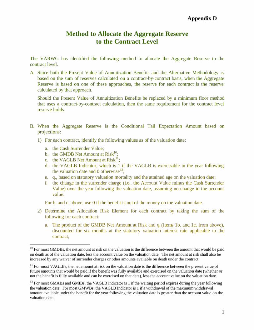
Appendix D

1

Method to Allocate the Aggregate Reserve to the Contract Level

The VARWG has identified the following method to allocate the Aggregate Reserve to the contract level.

A. Since both the Present Value of Annuitization Benefits and the Alternative Methodology is based on the sum of reserves calculated on a contract-by-contract basis, when the Aggregate Reserve is based on one of these approaches, the reserve for each contract is the reserve calculated by that approach.

Should the Present Value of Annuitization Benefits be replaced by a minimum floor method that uses a contract-by-contract calculation, then the same requirement for the contract level reserve holds.

B. When the Aggregate Reserve is the Conditional Tail Expectation Amount based on projections:

1) For each contract, identify the following values as of the valuation date:

a. the Cash Surrender Value; b. the GMDB Net Amount at RiskTPF

10FPT;

c. the VAGLB Net Amount at RiskTPF

11FPT;

d. the VAGLB Indicator, which is 1 if the VAGLB is exercisable in the year following the valuation date and 0 otherwiseTPF

12FPT;

e. qBxB, based on statutory valuation mortality and the attained age on the valuation date; f. the change in the surrender charge (i.e., the Account Value minus the Cash Surrender

Value) over the year following the valuation date, assuming no change in the account value.

For b. and c. above, use 0 if the benefit is out of the money on the valuation date.

2) Determine the Allocation Risk Element for each contract by taking the sum of the following for each contract:

a. The product of the GMDB Net Amount at Risk and qBx B(items 1b. and 1e. from above), discounted for six months at the statutory valuation interest rate applicable to the contract;

TP

10PT For most GMDBs, the net amount at risk on the valuation is the difference between the amount that would be paid

on death as of the valuation date, less the account value on the valuation date. The net amount at risk shall also be increased by any waiver of surrender charges or other amounts available on death under the contract.

TP

11PT For most VAGLBs, the net amount at risk on the valuation date is the difference between the present value of

future amounts that would be paid if the benefit was fully available and exercised on the valuation date (whether or not the benefit is fully available and can be exercised on that date), less the account value on the valuation date.

TP

12PT For most GMABs and GMIBs, the VAGLB Indicator is 1 if the waiting period expires during the year following

the valuation date. For most GMWBs, the VAGLB Indicator is 1 if a withdrawal of the maximum withdrawal amount available under the benefit for the year following the valuation date is greater than the account value on the valuation date.

Appendix D

2

b. The product of the VAGLB Net Amount at Risk, the VAGLB Indicator, and (1-qBxB) B

B(based on items 1c., 1d. and 1e. from above)TPF

13FPT, discounted for one year at the

statutory valuation interest rate applicable to the contract;

c. The product of the change in surrender charge and (1-qx) (based on items 1f. and 1e.from above), discounted for one year at the statutory valuation interest rate applicable to the contract.

Note that item a. is an approximation of the GMDB net amount at risk payable over the next year, item b. is an approximation of the VAGLB net amount at risk exercisable over the next year, and item c. is an approximation of the amortization of the surrender charge over the next year.

3) Determine the Aggregate Allocation Risk Element by taking the sum over all the contracts of the Allocation Risk Elements for each contract (from #2 above).

4) Subtract the sum of the Cash Surrender Values over all the contracts from the Aggregate Reserve.

5) Express the Aggregate Reserve in excess of Cash Surrender Value as a percentage of the Aggregate Allocation Risk Elements by taking the ratio of item #4 to item #3.

6) The allocated Aggregate Reserve for each contract is determined by applying the ratio in item #5 to the Allocation Risk Element for each contract (i.e., for each contract, multiply the result of item #2 by the ratio determined in item #5).

Note that if the Aggregate Reserve equals the aggregate Cash Surrender Value, the ratio in #5 is 0 and the reserve for each contract is the Cash Surrender Value.

C. Possible Alternatives

A possible alternative is to use the Present Value of Annuitization Benefits (or any minimum floor method that replaces it) in lieu of Cash Surrender Value in the above approach.

Other possible alternatives include projecting the items in #2 above over two or more years, and/or working in a drop/return scenario for the GMDB and VAGLB net amounts at risk. Note that this won't affect the Aggregate Reserve, it will only impact the allocation of the Aggregate Reserve among the contracts.

TP

13PT For contracts that have only a portion of the VAGLB that is exercisable over the next year, this product shall

reflect only the net amount at risk that is attributable to that portion of the VAGLB.

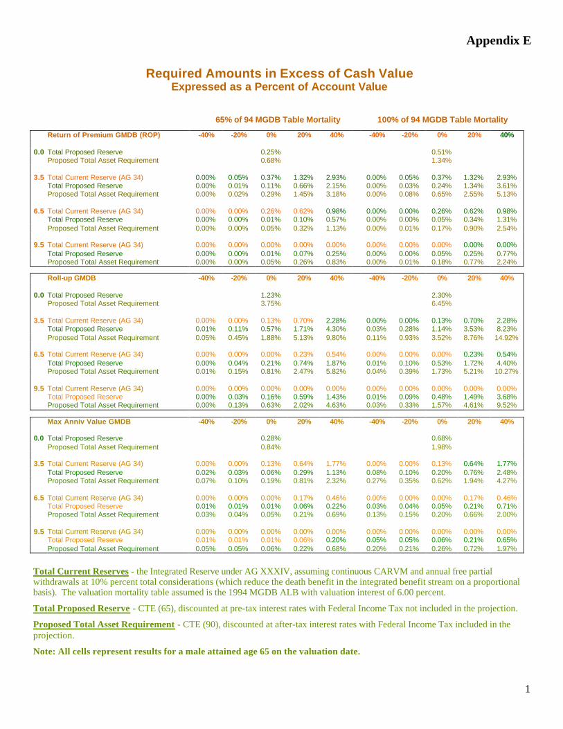
Appendix E

1

Required Amounts in Excess of Cash Value Expressed as a Percent of Account Value

65% of 94 MGDB Table Mortality 100% of 94 MGDB Table Mortality

Return of Premium GMDB (ROP) -40% -20% 0% 20% 40% -40% -20% 0% 20% 40% 0.0 Total Proposed Reserve 0.25% 0.51% Proposed Total Asset Requirement 0.68% 1.34%

3.5 Total Current Reserve (AG 34) 0.00% 0.05% 0.37% 1.32% 2.93% 0.00% 0.05% 0.37% 1.32% 2.93% Total Proposed Reserve 0.00% 0.01% 0.11% 0.66% 2.15% 0.00% 0.03% 0.24% 1.34% 3.61% Proposed Total Asset Requirement 0.00% 0.02% 0.29% 1.45% 3.18% 0.00% 0.08% 0.65% 2.55% 5.13%



Roll-up GMDB -40% -20% 0% 20% 40% -40% -20% 0% 20% 40% 0.0 Total Proposed Reserve 1.23% 2.30% Proposed Total Asset Requirement 3.75% 6.45%




Max Anniv Value GMDB -40% -20% 0% 20% 40% -40% -20% 0% 20% 40% 0.0 Total Proposed Reserve 0.28% 0.68% Proposed Total Asset Requirement 0.84% 1.98%




Total Current Reserves - the Integrated Reserve under AG XXXIV, assuming continuous CARVM and annual free partial withdrawals at 10% percent total considerations (which reduce the death benefit in the integrated benefit stream on a proportional basis). The valuation mortality table assumed is the 1994 MGDB ALB with valuation interest of 6.00 percent.

Total Proposed Reserve - CTE (65), discounted at pre-tax interest rates with Federal Income Tax not included in the projection.

Proposed Total Asset Requirement - CTE (90), discounted at after-tax interest rates with Federal Income Tax included in the projection.

Note: All cells represent results for a male attained age 65 on the valuation date.

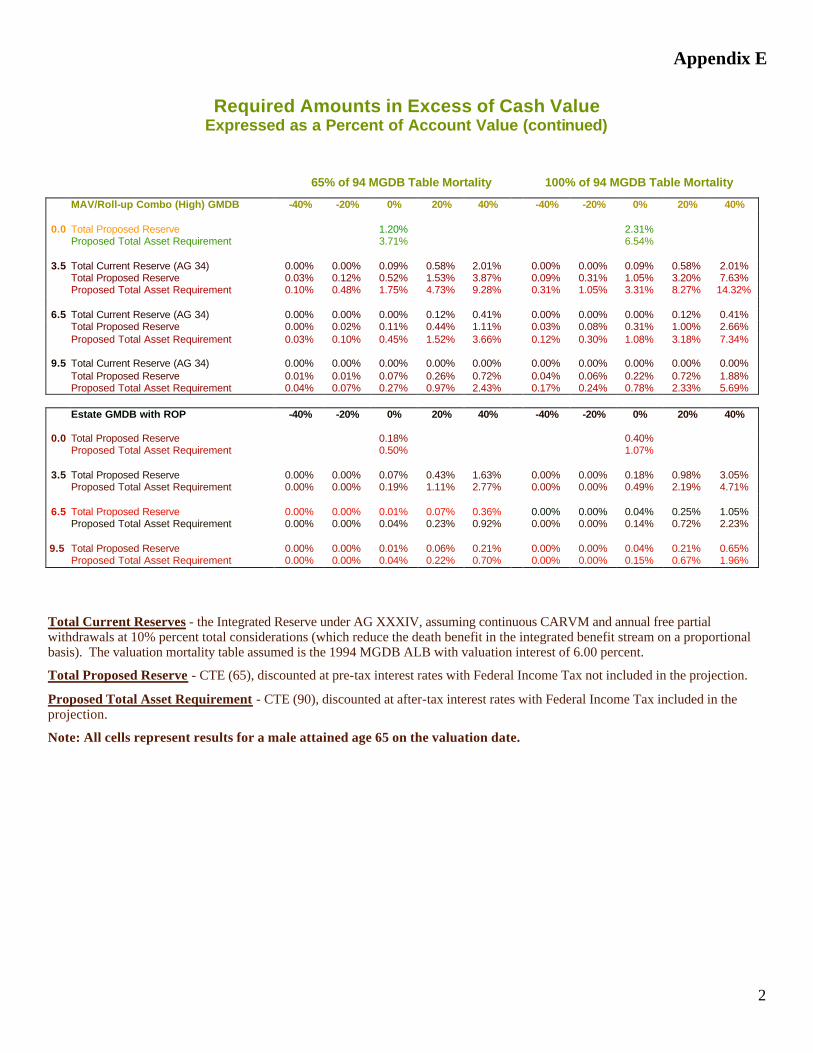
Appendix E

2

Required Amounts in Excess of Cash Value Expressed as a Percent of Account Value (continued)


MAV/Roll-up Combo (High) GMDB -40% -20% 0% 20% 40% -40% -20% 0% 20% 40% 0.0 Total Proposed Reserve 1.20% 2.31% Proposed Total Asset Requirement 3.71% 6.54%



9.5 Total Current Reserve (AG 34) 0.00% 0.00% 0.00% 0.00% 0.00% 0.00% 0.00% 0.00% 0.00% 0.00% Total Proposed Reserve 0.01% 0.01% 0.07% 0.26% 0.72% 0.04% 0.06% 0.22% 0.72% 1.88% Proposed Total Asset Requirement 0.04% 0.07% 0.27% 0.97% 2.43% 0.17% 0.24% 0.78% 2.33% 5.69% Estate GMDB with ROP -40% -20% 0% 20% 40% -40% -20% 0% 20% 40% 0.0 Total Proposed Reserve 0.18% 0.40% Proposed Total Asset Requirement 0.50% 1.07%

3.5 Total Proposed Reserve 0.00% 0.00% 0.07% 0.43% 1.63% 0.00% 0.00% 0.18% 0.98% 3.05% Proposed Total Asset Requirement 0.00% 0.00% 0.19% 1.11% 2.77% 0.00% 0.00% 0.49% 2.19% 4.71%



Total Current Reserves - the Integrated Reserve under AG XXXIV, assuming continuous CARVM and annual free partial withdrawals at 10% percent total considerations (which reduce the death benefit in the integrated benefit stream on a proportional basis). The valuation mortality table assumed is the 1994 MGDB ALB with valuation interest of 6.00 percent.




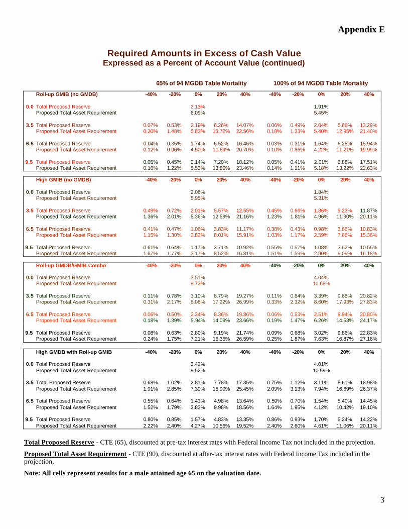
Appendix E

3

Required Amounts in Excess of Cash Value Expressed as a Percent of Account Value (continued)


Roll-up GMIB (no GMDB) -40% -20% 0% 20% 40% -40% -20% 0% 20% 40% 0.0 Total Proposed Reserve 2.13% 1.91% Proposed Total Asset Requirement 6.09% 5.45%




High GMIB (no GMDB) -40% -20% 0% 20% 40% -40% -20% 0% 20% 40% 0.0 Total Proposed Reserve 2.06% 1.84% Proposed Total Asset Requirement 5.95% 5.31%




Roll-up GMDB/GMIB Combo -40% -20% 0% 20% 40% -40% -20% 0% 20% 40% 0.0 Total Proposed Reserve 3.51% 4.04% Proposed Total Asset Requirement 9.73% 10.68%



9.5 Total Proposed Reserve 0.08% 0.63% 2.80% 9.19% 21.74% 0.09% 0.68% 3.02% 9.86% 22.83% Proposed Total Asset Requirement 0.24% 1.75% 7.21% 16.35% 26.59% 0.25% 1.87% 7.63% 16.87% 27.16% High GMDB with Roll-up GMIB -40% -20% 0% 20% 40% -40% -20% 0% 20% 40% 0.0 Total Proposed Reserve 3.42% 4.01% Proposed Total Asset Requirement 9.52% 10.59%







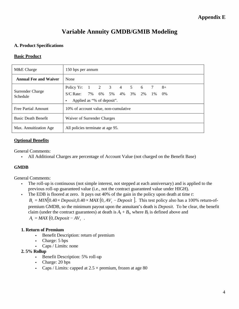
Appendix E

4

Variable Annuity GMDB/GMIB Modeling

A. Product Specifications Basic Product

M&E Charge 150 bps per annum

Annual Fee and Waiver None

Surrender Charge Schedule

Policy Yr: 1 2 3 4 5 6 7 8+

S/C Rate: 7% 6% 5% 4% 3% 2% 1% 0%

§ Applied as “% of deposit”.

Free Partial Amount 10% of account value, non-cumulative

Basic Death Benefit Waiver of Surrender Charges

Max. Annuitization Age All policies terminate at age 95.

Optional Benefits General Comments:

§ All Additional Charges are percentage of Account Value (not charged on the Benefit Base) GMDB General Comments:

§ The roll-up is continuous (not simple interest, not stepped at each anniversary) and is applied to the previous roll-up guaranteed value (i.e., not the contract guaranteed value under HIGH).

§ The EDB is floored at zero. It pays out 40% of the gain in the policy upon death at time t: ( )[ ]DepositAVMAXDepositMINB tt −××= ,040.0,40.0 . This test policy also has a 100% return-of-

premium GMDB, so the minimum payout upon the annuitant’s death is Deposit. To be clear, the benefit claim (under the contract guarantees) at death is ABt B + BBt B, where BBt B is defined above and

( )tt AVDepositMAXA −= ,0 .

1. Return of Premium § Benefit Description: return of premium § Charge: 5 bps § Caps / Limits: none

2. 5% Rollup § Benefit Description: 5% roll-up § Charge: 20 bps § Caps / Limits: capped at 2.5 × premium, frozen at age 80

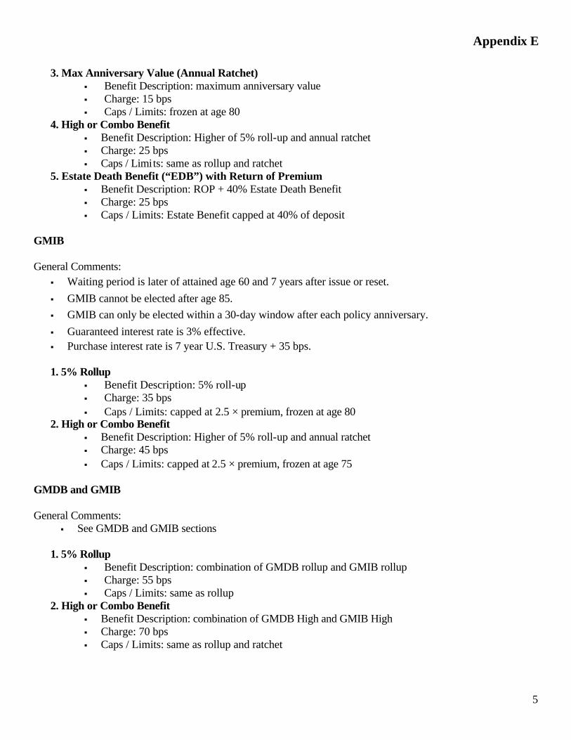
Appendix E

5

3. Max Anniversary Value (Annual Ratchet) § Benefit Description: maximum anniversary value § Charge: 15 bps § Caps / Limits: frozen at age 80

4. High or Combo Benefit § Benefit Description: Higher of 5% roll-up and annual ratchet § Charge: 25 bps § Caps / Limits: same as rollup and ratchet

5. Estate Death Benefit (“EDB”) with Return of Premium § Benefit Description: ROP + 40% Estate Death Benefit § Charge: 25 bps § Caps / Limits: Estate Benefit capped at 40% of deposit

GMIB General Comments:

§ Waiting period is later of attained age 60 and 7 years after issue or reset. § GMIB cannot be elected after age 85. § GMIB can only be elected within a 30-day window after each policy anniversary. § Guaranteed interest rate is 3% effective. § Purchase interest rate is 7 year U.S. Treasury + 35 bps.

1. 5% Rollup

§ Benefit Description: 5% roll-up § Charge: 35 bps § Caps / Limits: capped at 2.5 × premium, frozen at age 80

2. High or Combo Benefit § Benefit Description: Higher of 5% roll-up and annual ratchet § Charge: 45 bps § Caps / Limits: capped at 2.5 × premium, frozen at age 75

GMDB and GMIB General Comments:

§ See GMDB and GMIB sections

1. 5% Rollup § Benefit Description: combination of GMDB rollup and GMIB rollup § Charge: 55 bps § Caps / Limits: same as rollup

2. High or Combo Benefit § Benefit Description: combination of GMDB High and GMIB High § Charge: 70 bps § Caps / Limits: same as rollup and ratchet

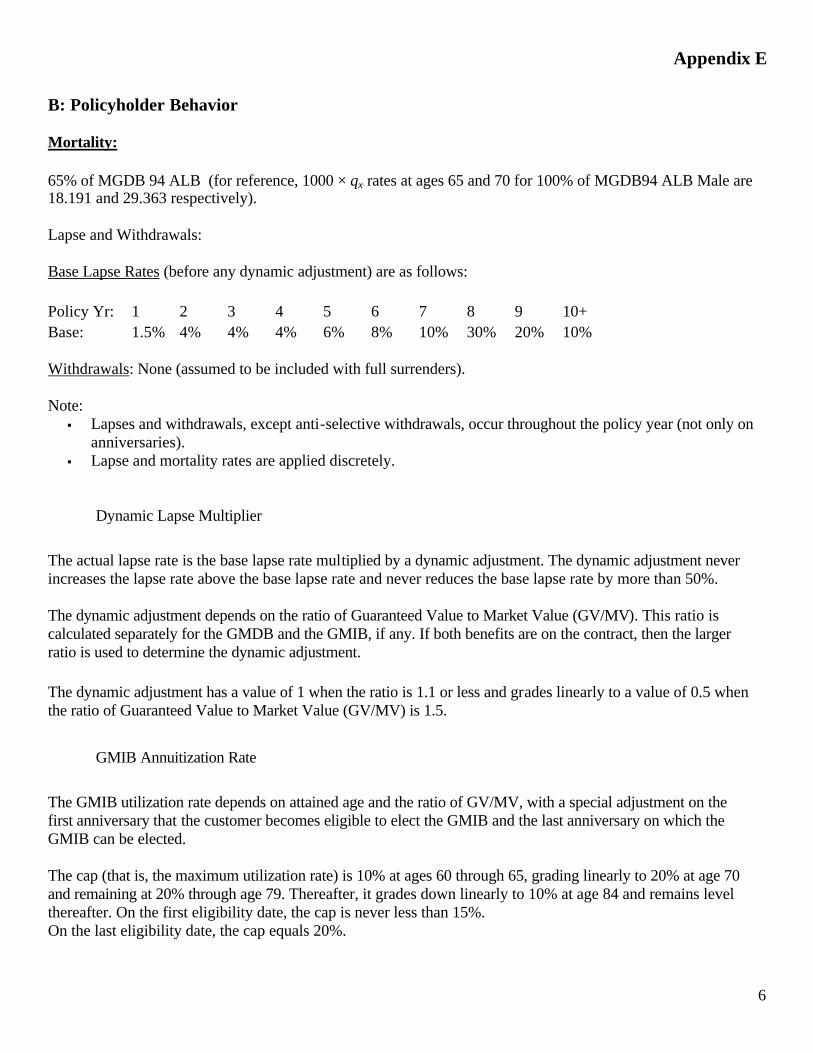
Appendix E

6

B: Policyholder Behavior Mortality: 65% of MGDB 94 ALB (for reference, 1000 × qBx B rates at ages 65 and 70 for 100% of MGDB94 ALB Male are 18.191 and 29.363 respectively). Lapse and Withdrawals: Base Lapse Rates (before any dynamic adjustment) are as follows: Policy Yr: 1 2 3 4 5 6 7 8 9 10+ Base: 1.5% 4% 4% 4% 6% 8% 10% 30% 20% 10% Withdrawals: None (assumed to be included with full surrenders). Note: § Lapses and withdrawals, except anti-selective withdrawals, occur throughout the policy year (not only on

anniversaries). § Lapse and mortality rates are applied discretely.

Dynamic Lapse Multiplier

The actual lapse rate is the base lapse rate multiplied by a dynamic adjustment. The dynamic adjustment never increases the lapse rate above the base lapse rate and never reduces the base lapse rate by more than 50%. The dynamic adjustment depends on the ratio of Guaranteed Value to Market Value (GV/MV). This ratio is calculated separately for the GMDB and the GMIB, if any. If both benefits are on the contract, then the larger ratio is used to determine the dynamic adjustment. The dynamic adjustment has a value of 1 when the ratio is 1.1 or less and grades linearly to a value of 0.5 when the ratio of Guaranteed Value to Market Value (GV/MV) is 1.5.

GMIB Annuitization Rate The GMIB utilization rate depends on attained age and the ratio of GV/MV, with a special adjustment on the first anniversary that the customer becomes eligible to elect the GMIB and the last anniversary on which the GMIB can be elected. The cap (that is, the maximum utilization rate) is 10% at ages 60 through 65, grading linearly to 20% at age 70 and remaining at 20% through age 79. Thereafter, it grades down linearly to 10% at age 84 and remains level thereafter. On the first eligibility date, the cap is never less than 15%. On the last eligibility date, the cap equals 20%.

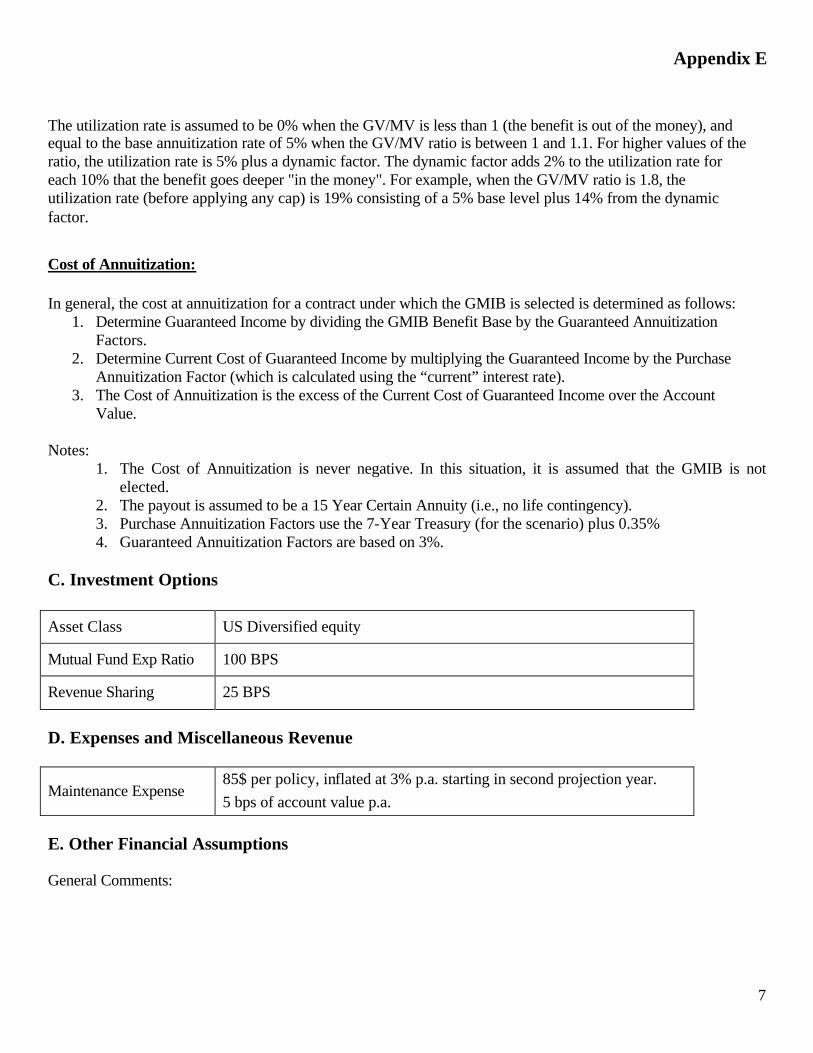
Appendix E

7

The utilization rate is assumed to be 0% when the GV/MV is less than 1 (the benefit is out of the money), and equal to the base annuitization rate of 5% when the GV/MV ratio is between 1 and 1.1. For higher values of the ratio, the utilization rate is 5% plus a dynamic factor. The dynamic factor adds 2% to the utilization rate for each 10% that the benefit goes deeper "in the money". For example, when the GV/MV ratio is 1.8, the utilization rate (before applying any cap) is 19% consisting of a 5% base level plus 14% from the dynamic factor. Cost of Annuitization: In general, the cost at annuitization for a contract under which the GMIB is selected is determined as follows:

1. Determine Guaranteed Income by dividing the GMIB Benefit Base by the Guaranteed Annuitization Factors.

2. Determine Current Cost of Guaranteed Income by multiplying the Guaranteed Income by the Purchase Annuitization Factor (which is calculated using the “current” interest rate).

3. The Cost of Annuitization is the excess of the Current Cost of Guaranteed Income over the Account Value.

Notes:

1. The Cost of Annuitization is never negative. In this situation, it is assumed that the GMIB is not elected.

2. The payout is assumed to be a 15 Year Certain Annuity (i.e., no life contingency). 3. Purchase Annuitization Factors use the 7-Year Treasury (for the scenario) plus 0.35% 4. Guaranteed Annuitization Factors are based on 3%.

C. Investment Options Asset Class US Diversified equity

Mutual Fund Exp Ratio 100 BPS

Revenue Sharing 25 BPS

D. Expenses and Miscellaneous Revenue

Maintenance Expense 85$ per policy, inflated at 3% p.a. starting in second projection year. 5 bps of account value p.a.

E. Other Financial Assumptions General Comments:

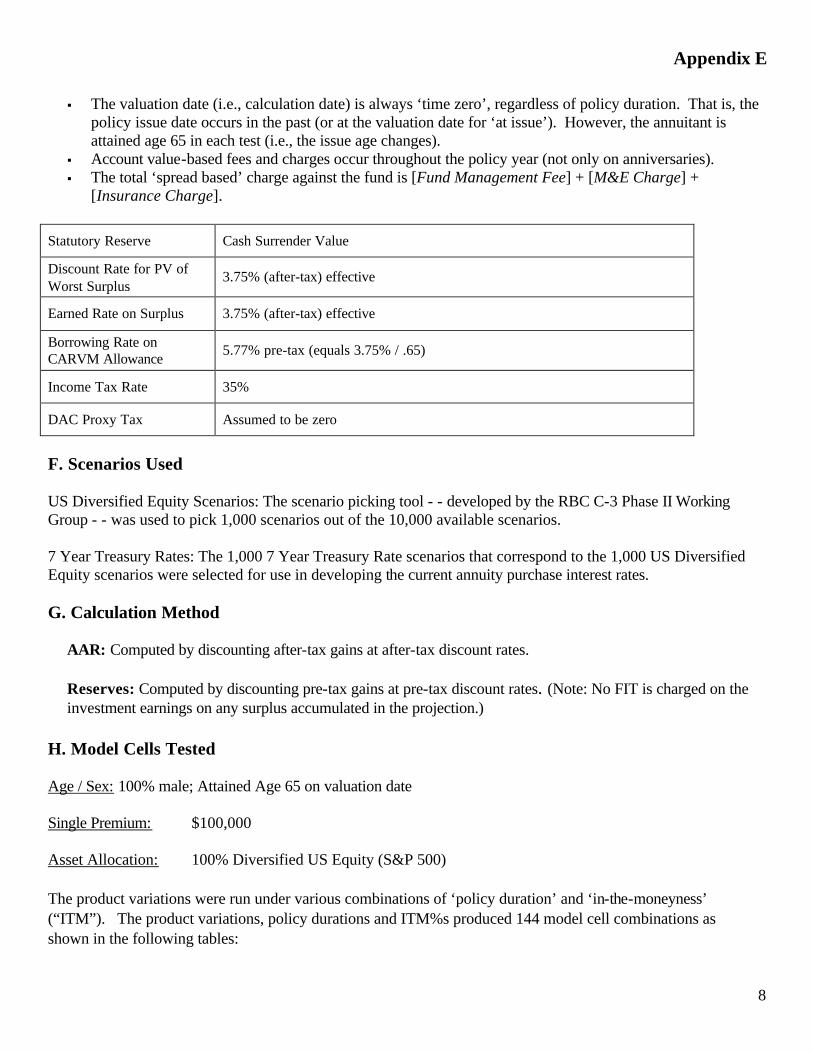
Appendix E

8

§ The valuation date (i.e., calculation date) is always ‘time zero’, regardless of policy duration. That is, the policy issue date occurs in the past (or at the valuation date for ‘at issue’). However, the annuitant is attained age 65 in each test (i.e., the issue age changes).

§ Account value-based fees and charges occur throughout the policy year (not only on anniversaries). § The total ‘spread based’ charge against the fund is [Fund Management Fee] + [M&E Charge] +

[Insurance Charge].

Statutory Reserve Cash Surrender Value

Discount Rate for PV of Worst Surplus

3.75% (after-tax) effective

Earned Rate on Surplus 3.75% (after-tax) effective

Borrowing Rate on CARVM Allowance

5.77% pre-tax (equals 3.75% / .65)

Income Tax Rate 35%

DAC Proxy Tax Assumed to be zero

F. Scenarios Used US Diversified Equity Scenarios: The scenario picking tool - - developed by the RBC C-3 Phase II Working Group - - was used to pick 1,000 scenarios out of the 10,000 available scenarios. 7 Year Treasury Rates: The 1,000 7 Year Treasury Rate scenarios that correspond to the 1,000 US Diversified Equity scenarios were selected for use in developing the current annuity purchase interest rates. G. Calculation Method

AAR: Computed by discounting after-tax gains at after-tax discount rates. Reserves: Computed by discounting pre-tax gains at pre-tax discount rates. (Note: No FIT is charged on the investment earnings on any surplus accumulated in the projection.)

H. Model Cells Tested Age / Sex: 100% male; Attained Age 65 on valuation date Single Premium: $100,000 Asset Allocation: 100% Diversified US Equity (S&P 500) The product variations were run under various combinations of ‘policy duration’ and ‘in-the-moneyness’ (“ITM”). The product variations, policy durations and ITM%s produced 144 model cell combinations as shown in the following tables:

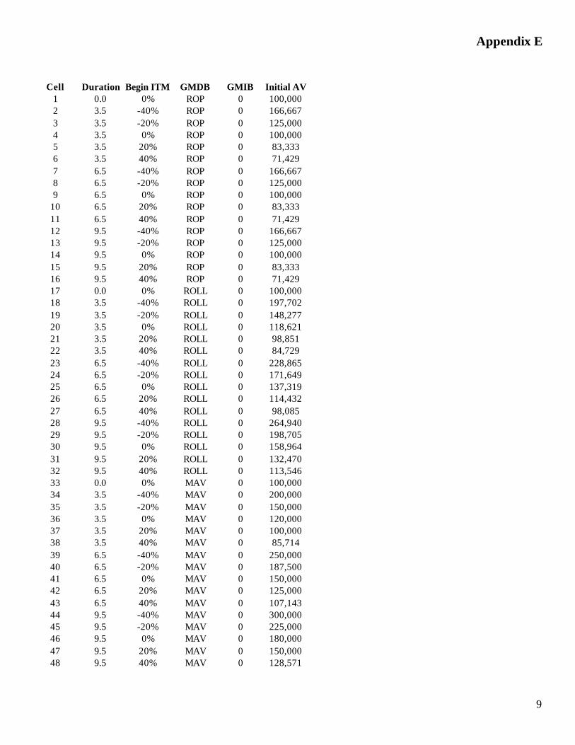
Appendix E

9

Cell Duration Begin ITM GMDB GMIB Initial AV

1 0.0 0% ROP 0 100,000 2 3.5 -40% ROP 0 166,667 3 3.5 -20% ROP 0 125,000 4 3.5 0% ROP 0 100,000 5 3.5 20% ROP 0 83,333 6 3.5 40% ROP 0 71,429 7 6.5 -40% ROP 0 166,667 8 6.5 -20% ROP 0 125,000 9 6.5 0% ROP 0 100,000

10 6.5 20% ROP 0 83,333 11 6.5 40% ROP 0 71,429 12 9.5 -40% ROP 0 166,667 13 9.5 -20% ROP 0 125,000 14 9.5 0% ROP 0 100,000 15 9.5 20% ROP 0 83,333 16 9.5 40% ROP 0 71,429 17 0.0 0% ROLL 0 100,000 18 3.5 -40% ROLL 0 197,702 19 3.5 -20% ROLL 0 148,277 20 3.5 0% ROLL 0 118,621 21 3.5 20% ROLL 0 98,851 22 3.5 40% ROLL 0 84,729 23 6.5 -40% ROLL 0 228,865 24 6.5 -20% ROLL 0 171,649 25 6.5 0% ROLL 0 137,319 26 6.5 20% ROLL 0 114,432 27 6.5 40% ROLL 0 98,085 28 9.5 -40% ROLL 0 264,940 29 9.5 -20% ROLL 0 198,705 30 9.5 0% ROLL 0 158,964 31 9.5 20% ROLL 0 132,470 32 9.5 40% ROLL 0 113,546 33 0.0 0% MAV 0 100,000 34 3.5 -40% MAV 0 200,000 35 3.5 -20% MAV 0 150,000 36 3.5 0% MAV 0 120,000 37 3.5 20% MAV 0 100,000 38 3.5 40% MAV 0 85,714 39 6.5 -40% MAV 0 250,000 40 6.5 -20% MAV 0 187,500 41 6.5 0% MAV 0 150,000 42 6.5 20% MAV 0 125,000 43 6.5 40% MAV 0 107,143 44 9.5 -40% MAV 0 300,000 45 9.5 -20% MAV 0 225,000 46 9.5 0% MAV 0 180,000 47 9.5 20% MAV 0 150,000 48 9.5 40% MAV 0 128,571

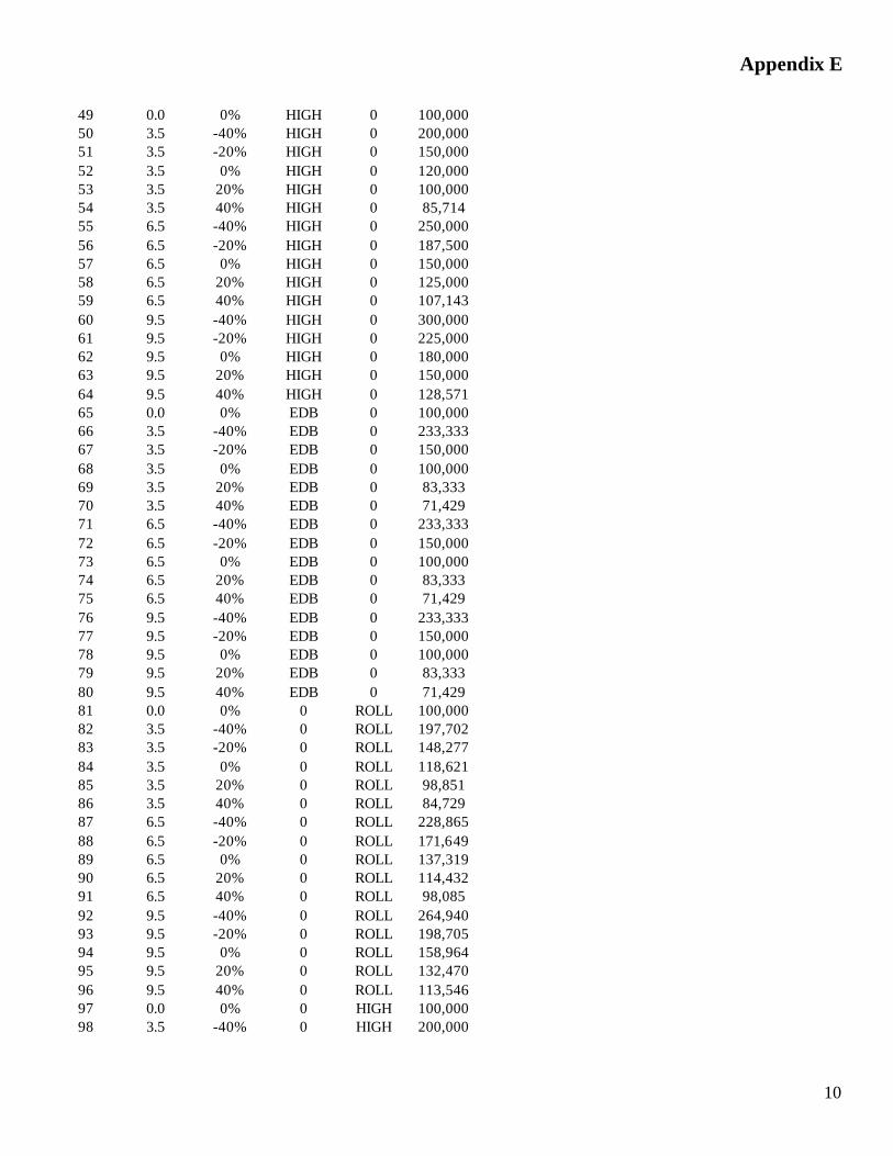
Appendix E

10

49 0.0 0% HIGH 0 100,000 50 3.5 -40% HIGH 0 200,000 51 3.5 -20% HIGH 0 150,000 52 3.5 0% HIGH 0 120,000 53 3.5 20% HIGH 0 100,000 54 3.5 40% HIGH 0 85,714 55 6.5 -40% HIGH 0 250,000 56 6.5 -20% HIGH 0 187,500 57 6.5 0% HIGH 0 150,000 58 6.5 20% HIGH 0 125,000 59 6.5 40% HIGH 0 107,143 60 9.5 -40% HIGH 0 300,000 61 9.5 -20% HIGH 0 225,000 62 9.5 0% HIGH 0 180,000 63 9.5 20% HIGH 0 150,000 64 9.5 40% HIGH 0 128,571 65 0.0 0% EDB 0 100,000 66 3.5 -40% EDB 0 233,333 67 3.5 -20% EDB 0 150,000 68 3.5 0% EDB 0 100,000 69 3.5 20% EDB 0 83,333 70 3.5 40% EDB 0 71,429 71 6.5 -40% EDB 0 233,333 72 6.5 -20% EDB 0 150,000 73 6.5 0% EDB 0 100,000 74 6.5 20% EDB 0 83,333 75 6.5 40% EDB 0 71,429 76 9.5 -40% EDB 0 233,333 77 9.5 -20% EDB 0 150,000 78 9.5 0% EDB 0 100,000 79 9.5 20% EDB 0 83,333 80 9.5 40% EDB 0 71,429 81 0.0 0% 0 ROLL 100,000 82 3.5 -40% 0 ROLL 197,702 83 3.5 -20% 0 ROLL 148,277 84 3.5 0% 0 ROLL 118,621 85 3.5 20% 0 ROLL 98,851 86 3.5 40% 0 ROLL 84,729 87 6.5 -40% 0 ROLL 228,865 88 6.5 -20% 0 ROLL 171,649 89 6.5 0% 0 ROLL 137,319 90 6.5 20% 0 ROLL 114,432 91 6.5 40% 0 ROLL 98,085 92 9.5 -40% 0 ROLL 264,940 93 9.5 -20% 0 ROLL 198,705 94 9.5 0% 0 ROLL 158,964 95 9.5 20% 0 ROLL 132,470 96 9.5 40% 0 ROLL 113,546 97 0.0 0% 0 HIGH 100,000 98 3.5 -40% 0 HIGH 200,000

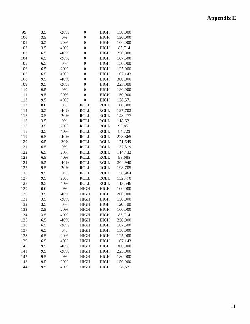
Appendix E

11

99 3.5 -20% 0 HIGH 150,000 100 3.5 0% 0 HIGH 120,000 101 3.5 20% 0 HIGH 100,000 102 3.5 40% 0 HIGH 85,714 103 6.5 -40% 0 HIGH 250,000 104 6.5 -20% 0 HIGH 187,500 105 6.5 0% 0 HIGH 150,000 106 6.5 20% 0 HIGH 125,000 107 6.5 40% 0 HIGH 107,143 108 9.5 -40% 0 HIGH 300,000 109 9.5 -20% 0 HIGH 225,000 110 9.5 0% 0 HIGH 180,000 111 9.5 20% 0 HIGH 150,000 112 9.5 40% 0 HIGH 128,571 113 0.0 0% ROLL ROLL 100,000 114 3.5 -40% ROLL ROLL 197,702 115 3.5 -20% ROLL ROLL 148,277 116 3.5 0% ROLL ROLL 118,621 117 3.5 20% ROLL ROLL 98,851 118 3.5 40% ROLL ROLL 84,729 119 6.5 -40% ROLL ROLL 228,865 120 6.5 -20% ROLL ROLL 171,649 121 6.5 0% ROLL ROLL 137,319 122 6.5 20% ROLL ROLL 114,432 123 6.5 40% ROLL ROLL 98,085 124 9.5 -40% ROLL ROLL 264,940 125 9.5 -20% ROLL ROLL 198,705 126 9.5 0% ROLL ROLL 158,964 127 9.5 20% ROLL ROLL 132,470 128 9.5 40% ROLL ROLL 113,546 129 0.0 0% HIGH HIGH 100,000 130 3.5 -40% HIGH HIGH 200,000 131 3.5 -20% HIGH HIGH 150,000 132 3.5 0% HIGH HIGH 120,000 133 3.5 20% HIGH HIGH 100,000 134 3.5 40% HIGH HIGH 85,714 135 6.5 -40% HIGH HIGH 250,000 136 6.5 -20% HIGH HIGH 187,500 137 6.5 0% HIGH HIGH 150,000 138 6.5 20% HIGH HIGH 125,000 139 6.5 40% HIGH HIGH 107,143 140 9.5 -40% HIGH HIGH 300,000 141 9.5 -20% HIGH HIGH 225,000 142 9.5 0% HIGH HIGH 180,000 143 9.5 20% HIGH HIGH 150,000 144 9.5 40% HIGH HIGH 128,571

Appendix G

Volatility of Total Asset Requirement

The capital developed by the methodology defined herein can vary substantially from period to period due to market movements. Although we believe this is consistent with most financial economic models (e.g., option prices are also volatile under similar circumstances for similar reasons), and that this volatility may properly encourage companies to address the risk management issues associated with these products, the question as to whether the RBC regulatory tool should reflect something other than the specific economic values at only one point in time. The Subcommittee has not taken a position on this, but has given some thought as to methods by which such a standard could be achieved without sacrificing the integrity of the results. The following discusses some possible alternatives.

At a high level, there are two obvious choices for achieving less volatile results: “Input Methods” versus “Output Methods”. Input Methods rely on using “adjusted asset values” as inputs to the methodology. In this case, account values do not fully reflect all market values at only one point in time. Output Methods start with the current point in time asset value, but use a technique to dampen movement in the final result. We believe that Input Methods are undesirable because they conceal the current economic situation in a way that is not “transparent” and are problematic for ratcheting (resetting) guarantees.

Some methods for Adjusting Output include:

i) Use a range for CTE(a) (say, 0.85 = a = 0.95) in such a way that it tempers the swings in capital requirements. The a -level would be objectively defined and not subject to discretion or manipulation.

ii) Using a weighted average of capital standards over a period of time (e.g., weighted average of the current quarter result and the previous three quarter-ends), perhaps in combination with some absolute CTE floor as a lower bound.

iii) Take advantage of “good” fluctuations to build a buffer that would then be gradually released. For example, if capital requirements decline due to improved equity prices, add 80% of the capital reduction back to the new lower number, but with a 95 CTE ceiling, then release the buffer over time. An AVR type structure could accomplish this.

It should be recognized that none of these methods is “theoretically based”. Instead, they reflect the potential problems inherent in setting a regulatory requirement based on values at a single point in time, with the potential volatility this implies. These methods simply illustrate ways to produce a smoother pattern of changes in regulatory requirements without materially affecting the underlying trend. If such adjustments are deemed appropriate, we tend to favor adjusting outputs as this method has the advantage of allowing the true loss distribution to be observed.

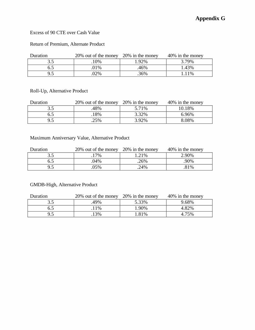
Appendix G

Excess of 90 CTE over Cash Value Return of Premium, Alternate Product Duration 20% out of the money 20% in the money 40% in the money

3.5 .10% 1.92% 3.79% 6.5 .01% .46% 1.43% 9.5 .02% .36% 1.11%

Roll-Up, Alternative Product Duration 20% out of the money 20% in the money 40% in the money

3.5 .48% 5.71% 10.18% 6.5 .18% 3.32% 6.96% 9.5 .25% 3.92% 8.08%

Maximum Anniversary Value, Alternative Product Duration 20% out of the money 20% in the money 40% in the money

3.5 .17% 1.21% 2.90% 6.5 .04% .26% .90% 9.5 .05% .24% .81%

GMDB-High, Alternative Product Duration 20% out of the money 20% in the money 40% in the money

3.5 .49% 5.33% 9.68% 6.5 .11% 1.90% 4.82% 9.5 .13% 1.81% 4.75%

APPENDIX H

1

Variable Annuity Reserve Work Group Analysis: Promulgating the New Reserve Method for Variable Annuities

In this document, the Variable Annuity Reserve Work Group (VARWG) of the American Academy of Actuaries is presenting the results of its analysis regarding the advantages and disadvantages of the three possible approaches to promulgating the new reserve requirements described in the VARWG’s June 2003 Report: Adoption of i) an actuarial guideline, ii) a model regulation pursuant to Section 9 of the Standard Valuation Law, or iii) a new or modified model law. During the June 2003 LHATF meeting, the VARWG discussed a timeline for adoption of the new requirements. The timeline presented is shown below. In order to meet this timeline, it would be necessary that LHATF decide soon which of the three approaches to promulgating the new reserve requirements it would most like to pursue. This is because the VARWG will need time to draft suggested language for the law, regulation or guideline for the December 2003 LHATF meeting. In addition, certain issues depend on which option is chosen, such as applicability of the new reserve method to in force contracts. The following timeline shows the sequence of events the VARWG anticipates in order for the new requirements to be adopted in a timely manner. Adopting this timeline would mean that as of the August 21, 2003 LHATF conference call, there would be approximately four months time for the VARWG work to be completed. There are three approaches being discussed by the VARWG:

1. Adopt the new method as an actuarial guideline such that the new method is considered a new interpretation of Commissioners’ Annuity Reserve Method (CARVM) for variable annuities.

2. Adopt the new method as a model regulation under Section 9 of the NAIC Model

Standard Valuation Law (SVL) such that the proposed reserve method becomes the reserve method for variable annuities. The approach of using a model regulation might also require an actuarial guideline to specify the details of the method and clarify its applications.

APPENDIX H

2

3. Incorporate the new method in a new subsection to SVL such that the new reserve method is identified in SVL as the reserve method for variable annuities. This approach would likely require a model regulation or an actuarial guideline to specify the details of the method and clarify its applications.

(The remainder of this appendix summarizes the practical implications of these three approaches.)

I. Adopt the New Method as an Actuarial Guideline An AG could be adopted as a revised interpretation of section 5a of the SVL. Alternatively, it could be adopted as an interpretation of section 6E of the NAIC Variable Annuity Model Regulation (VA Model Reg), which states that

The reserve liability for variable annuities shall be established pursuant to the requirements of the Standard Valuation Law in accordance with actuarial procedures that recognize the variable nature of the benefits provided and any mortality guarantees.

Advantages of adopting the new method as an actuarial guideline interpreting CARVM include, but are not limited to, the following:

• The new requirements can become effective in the shortest amount of time, • The effective date of the new requirements would be the same in almost all states, • Uniform reserve guidance among states,

• The new requirements can be applied to all inforce variable annuity contracts on a

statutory basis, if it is desired, and

• Subsequent modifications can be made more easily and quickly. Potential obstacles to adopting the new method as an actuarial guideline are:

1. As there are fundamental differences between the new reserve method and current CARVM, it may be difficult to justify adopting the new reserve method as an interpretation of CARVM through an actuarial guideline. Fundamental differences between the new reserve method and the current CARVM include (a) using a model-based approach incorporating assumptions regarding various aspects of policyholder behavior, (b) incorporating "renewal premiums" not required to be paid and company expenses, (c) using best estimate mortality assumptions rather than standardized mortality tables, and (d) discounting reserves at interest rates other than those specified in the Standard Valuation Law.

APPENDIX H

3

2. Current CARVM emphasizes the concept of greatest present value of guaranteed benefits. The new reserve method uses the conditional tail expectation (CTE) applied to the greatest of projected future losses for each stochastic scenario. One may argue that CTE deviates from the greatest present value of guaranteed benefit concept. A counter-argument is that the CTE measure is based on a comparable concept because the new method focuses on the greatest present value of projected losses under a variety of stochastic scenarios.

3. If the new method is promulgated as an actuarial guideline to be applicable to inforce

contracts, it may not ultimately prove to be the method required by the US Department of the Treasury (Treasury) for the calculation of tax reserves on inforce contracts due to Treasury positions recently taken.

4. If the new method is promulgated as an actuarial guideline, the scope of applicability of

the new method may be limited by the current scope of CARVM (in the case of an actuarial guideline that reinterprets section 5a of the SVL) or may only apply to variable annuities (in the case of an actuarial guideline that interprets the VA Model Reg). That is, contracts such as group life contracts insuring benefit guarantees of mutual fund customers that are not subject to current CARVM may not be subject to the new reserve method.

II. Adopting the New Method as a Model Regulation Under Section 9 of the

Standard Valuation Law This approach specifies the new method is an enhancement of the current CARVM for variable annuities. Because the technical aspects of the new reserve method may be too complicated to be included in a model regulation, this approach would likely require the NAIC to adopt a supporting actuarial guideline. Section 9 of the SVL states that

In the case of a plan of life insurance that provides for future premium determination, the amounts of which are to be determined by the insurance company based on then estimates of future experience, or in the case of a plan of life insurance or annuity that is of such a nature that the minimum reserve cannot be determined by the methods described in Section 5, 5a, and 8, the reserves that are held under the plan shall: A. Be appropriate in relation to the benefits and the pattern of premiums for that plan;

and B. Be computed by a method that is consistent with the principles of this Standard

Valuation Law, as determined by regulations promulgated by the commissioner.

APPENDIX H

4

Thus, the law specifies that if the minimum reserve for a contract cannot be determined using methods specified in the SVL (e.g., CARVM under Section 5a) due to the nature of the underlying contract, a different reserve methodology may be used to calculate the minimum reserve for the contract if the reserve method satisfies conditions (A) and (B) stated above. Condition (A) calls for appropriate recognition of benefits and premium patterns. Benefits would include guaranteed living and death benefits, and other benefits as well. Condition (A) may also be used to argue for the recognition of renewal premiums, as are recognized under the new reserve method. Condition (B) requires the reserve method to be consistent with the principles of the SVL, as determined by regulations and promulgated by commissioners. The language in the VA Model Reg (see section I. above) may further support using this approach. Advantages of adopting the new method as a model regulation include, but are not limited to, the following:

• The new method is considered a new reserve valuation method for variable annuities and any fundamental differences between the new method and current CARVM are irrelevant if it is adopted as a new model regulation, and

• The scope of applicability of the new method may be expanded to include contracts that

are currently not subject to CARVM such as the group life contracts described earlier. Practical challenges of adopting the new reserve method with reference to section 9 of SVL include, but are not limited to, the following:

1. The adoption of a model regulation with reference to the SVL may be time consuming and may not achieve uniformity among states in the reserve requirements ultimately adopted.

2. The timing of adoption of the new regulation could result in varying reserve requirements

on a state-by-state basis over time.

3. It is unclear whether a model regulation could be applied to all inforce variable annuity contracts, if that is desired.

APPENDIX H

5

III. Adopting the New Method as a New Section of the Standard Valuation Law

The third approach is similar to the second approach discussed above in that it also suggests that the proposed method is an enhancement of the current CARVM for variable annuities. The approach involves amending the SVL to specify new reserve requirements for variable annuity business. Under this approach, a new section would be added to the SVL (Section 5b, say) requiring the new reserve method. Because the technical aspects of the new reserve method will likely be too complicated to be included in the SVL, this approach would likely require the NAIC to adopt a supporting actuarial guideline. Major advantages of this approach include:

• The new method is considered a new reserve valuation method for variable annuities and any fundamental differences between the new method and current CARVM are irrelevant if it is promulgated as a revision to the model SVL, and

• Expansion of scope to cover other guarantees of benefits such as those provided under

the group life contracts described earlier. Potential difficulties related to the third approach are comparable but slightly different from the second approach. They include the following:

1. Adopting an amended model law can be even more time consuming than adopting a new model regulation.

2. It is unclear whether a revision to the model SVL could be applied to all inforce variable

annuity contracts, if that is desired. However, one area of precedence may be the change to the model SVL that incorporated the requirement for an actuarial opinion and memorandum (Section 3), which did apply to business already inforce.

3. May be more difficult to make subsequent modifications. However, this can be mitigated

by having the details appear in a supporting actuarial guideline.

4. Other unrelated proposed changes to the SVL may produce additional delays, both in construction of the model law and in adoption by the various states.

5. Some states may modify the model law during the adoption process, which would result

in a lack of uniformity by state.