PHENIX Drift Chamber operation principles

Modified by Victor RiabovFocus meeting

01/06/04

Original by Sergey ButsykFocus meeting

01/14/03

Outline Drift chamber (DCH) design Construction and assembling Operation principles Calibration aspects Trackfinding principles Future goals

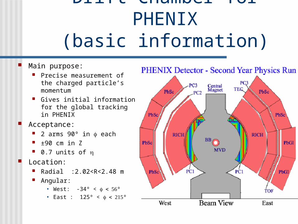
Drift Chamber for PHENIX(basic information)

Main purpose: Precise measurement of the

charged particle’s momentum

Gives initial information for the global tracking in PHENIX

Acceptance: 2 arms 90º in each ±90 cm in Z 0.7 units of

Location: Radial :2.02<R<2.48 m Angular:

• West: -34º < º• East : 125º < º

Drift Chamber design

DCH Frame

Wires

Keystone Made of titanium Conists of 20

identical keystones Weight ~ 1.5 tons Total tension of

wires ~ 3 tons

Lay-out of one keystone

6 radial layers of nets (X1,U1,V1,X2,U2,V2)

Stereo nets start in one keystone (n) and end in the neighbouring keystone e.g. (n+1) for U, (n-1) for V

The tilt of UV nets along allows measurement of Z component of the track

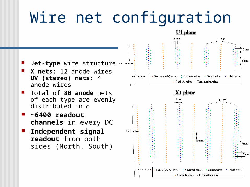
Wire net configuration

Jet-type wire structure X nets: 12 anode wires

UV (stereo) nets: 4 anode wires

Total of 80 anode nets of each type are evenly distributed in

~6400 readout channels in every DC

Independent signal readout from both sides (North, South)

Construction and assembling

Mechanical design and production – PNPI (Russia)

Front Electronics – SUNYSB Wire net production,

assembling - PNPI,SUNYSB

DCH Operation Principles To reconstruct charged particle track DC samples a few points in

space along the path of the particle. One such point is called a “HIT” Registration of one HIT is based on a few physical processes:

When charged particle transverse the gas volume of the DC it creates clusters of primary ionization on its way

Electrons of primary ionization drift from the point of ionization to anode wires along electric field lines

Electrons of primary ionization create avalanches in the vicinity of anode wires

Back drift of posistively charged ions generate measurable signal on anode wires which is amplified, shaped and discriminated

To register a HIT in the DC: Carry out drift time measurements: Start - collision time measured by

BBC; Stop - time when signal appears on the anode wire Drift time (t) can be tranformed into drift distance (x) if calibration curve

is known x = x(t) Working gas is chosen to have an uniform drift velocity in the active

region linear xt relation can be used x = Vdr · t

Gas mixture choice

50% Ar - 50% C2H6 mixture is chosen for operation based on: uniform drift velocity at E~1

kV/cm High Gas Gain Low diffusion coefficients

In Year2 ~1.6% Ethanol was added to the mixture to reduce ageing and improve HV properties of the nets

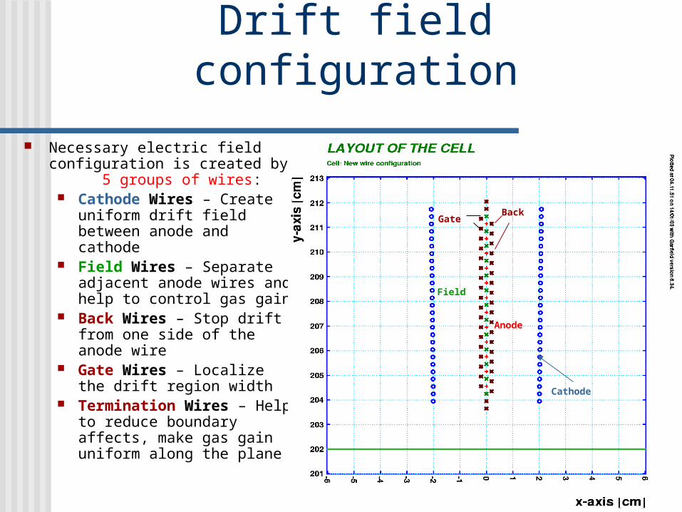
Drift field configuration

Necessary electric field configuration is created by 5 groups of wires:

Cathode Wires – Create uniform drift field between anode and cathode

Field Wires – Separate adjacent anode wires and help to control gas gain

Back Wires – Stop drift from one side of the anode wire

Gate Wires – Localize the drift region width

Termination Wires – Help to reduce boundary affects, make gas gain uniform along the plane

Cathode

BackGate

Anode

Field

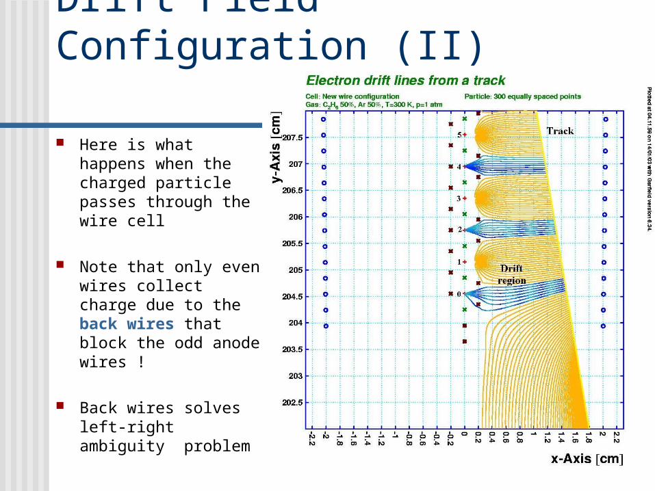
Drift Field Configuration (II)

Here is what happens when the charged particle passes through the wire cell

Note that only even wires collect charge due to the back wires that block the odd anode wires !

Back wires solves left-right ambiguity problem

DCH Performance (Run03) Single wire efficiency ~ 90-95% Back efficiency (probability to get hit

from the back closed side) < 10% Spatial Resolution ~ 120 um Angular resolution d/ ~ 1 mrad

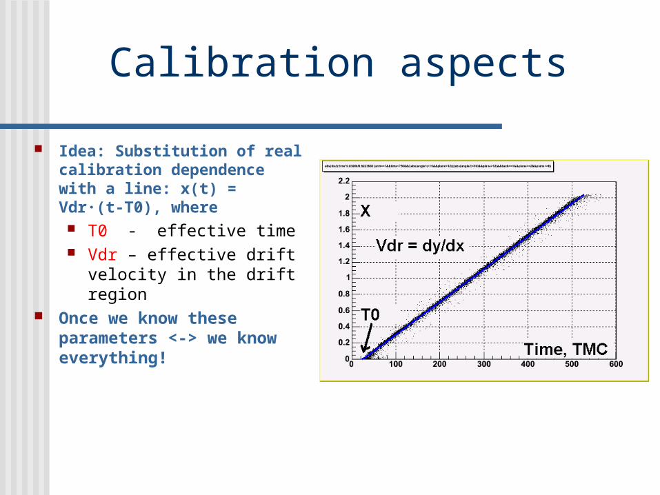
Calibration aspects

Idea: Substitution of real calibration dependence with a line: x(t) = Vdr·(t-T0), where T0 - effective time Vdr – effective drift

velocity in the drift region Once we know these

parameters <-> we know everything!

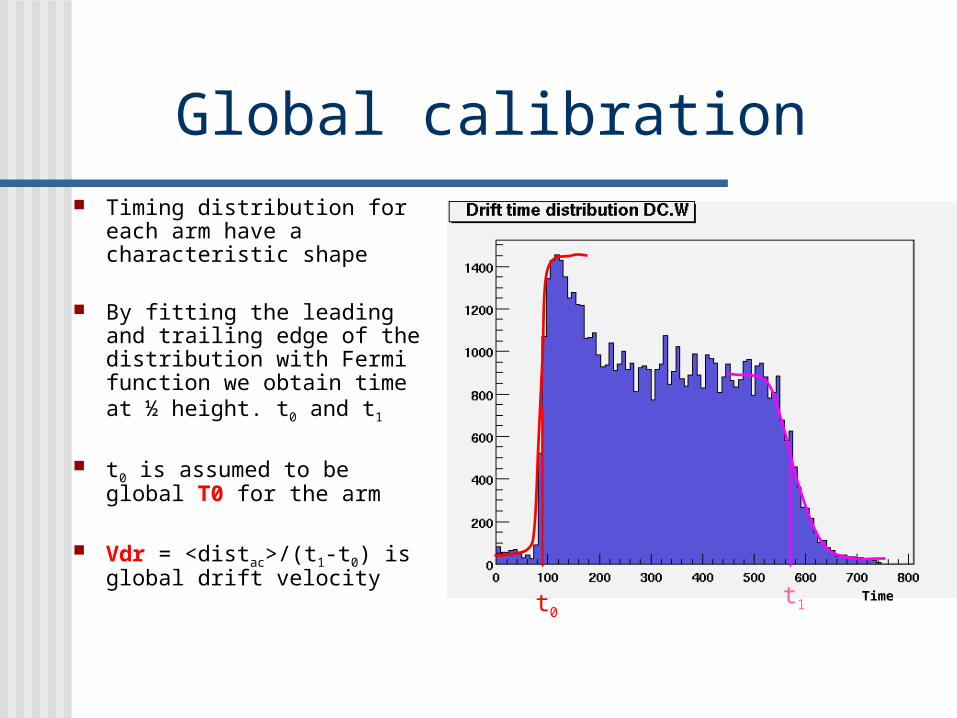
Global calibration Timing distribution for

each arm have a characteristic shape

By fitting the leading and trailing edge of the distribution with Fermi function we obtain time at ½ height. t0 and t1

t0 is assumed to be global T0 for the arm

Vdr = <distac>/(t1-t0) is global drift velocity t0

t1Time

Other calibration effectstaken into account

Slewing corrections – dependence of measured arrival time on the signal width

Shape of the drift region – the wires close to the mylar windows experience distortion of the electric field

Wire-by-wire t0 corrections – includes geometrical shifts of the anode wires within the net, electronics channel-by-channel variations e.t.c

Plane-by-plane Vdr corrections – Vdr is electric field dependant, thus it changes significantly on the side-standing wires where edge effects distorts the field strength

Global alignment to the vertex – center of the arm can be shifted from the vertex location. Translation of the arm center can be found by centering a distribution of the vertexes around zero in field-off data

Residual distributions

Pick hits of the track on 3 neighboring wires (i.e. 1,3,5). Residual for wire #3 is: x3 = (x1 + x5)/2 – x3

Residual is equal to ZERO if hits are perfectly aligned

Basic idea of local calibrations is to center all residuals at zero for all the parameters (i.e. align ever three neighboring wires)

Slewing corrections Look at residuals vs. width

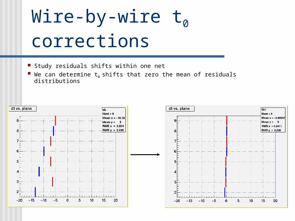
Wire-by-wire t0 corrections Study residuals shifts within one net We can determine t0 shifts that zero the mean of residuals distributions

Shape of the drift region The shape of the drift region was simulated in GARFIELD

and parameterized in the offline software

Tracking principlesMain assumptions:

• Track is straight in the detector region

and variables defined on the figure

•Use hough transform – calculate and for all possible combinations of hits and bin those values into hough array – 2D histogram on and

• Look for local maxima in hough array that surpass the threshold

Track Candidates

The results of the hough transform are track candidates

First we look for tracks with X1 and X2 hits

Remaining unassociated hits goes into X1 only and X2 only tracking

Finally we left with the following tracks

Z coordinates of tracks are dedined by PC1-UV-vertex tracking

Final results

Future goals Calibration of the detector is a main

contributor to the momentum resolution need to improve the absolute calibration methods Use outer detector’s matching Online Calibration

Improve HV stability over the run Control gas mixture properties during the

run Improve UV reconstruction