Physical impacts of land use in product life cycle assessment

Final report of the EURENVIRON-LCAGAPS sub-project on land use

Bo P. Weidema with contributions from Erwin Lindeijer

2001.12.31 Department of Manufacturing Engineering and Management Technical University of Denmark

IPL-033-01 Prepared as part of the EUREKA project EUROENVIRON 1296 LCAGAPS, sponsored by the Danish Agency for Industry and Trade

Weidema B P1 & Lindeijer E2 (2001). Physical impacts of land use in product life cycle assessment. Final report of the EURENVIRON-LCAGAPS sub-project on land use. Publisher: Department of Manufacturing Engineering and Management, Technical University of Denmark, Lyngby. Project funded by The Danish Agency for Industry and Trade as part of EUREKA project EU-1296 Current addresses of authors: 12.-0 LCA consultants, Borgergade 6, 1.,

1300 København K., Denmark 2TNO Industry, Sustainable Product

Development Department, PO Box 6031, 2600 JA Delft, The Netherlands

Page 3 of 52

Table of Contents

INTRODUCTION .................................................................................................................................... 4

EXECUTIVE SUMMARY ................................................................................................................. 5

1. CONCEPTS AND DEFINITIONS ......................................................................................... 6

1.1 LAND USE AND PHYSICAL IMPACTS................................................................................................................ 6 1.2 WHAT IS NOT INCLUDED HERE (RELATIONSHIP TO OTHER IMPACT CATEGORIES)............................................ 7 1.3 IMPACT CHAIN................................................................................................................................................ 8

1.3.1 The starting point: Boundary between inventory analysis and impact assessment ................................ 8 1.3.2 The end points: Areas of protection........................................................................................................ 9 1.3.3 Mid-points of the impact chain ............................................................................................................. 11

1.4 OCCUPATION AND TRANSFORMATION OF LAND............................................................................................ 13 1.5 CHOICE OF REFERENCE STATE FOR THE MEASUREMENT OF OCCUPATION IMPACTS....................................... 15 1.6 CHANGES IN THE RATE OF RELAXATION....................................................................................................... 18

2. INDICATORS FOR MEASURING NATURE VALUE ....................................... 19

2.1 SUBSTANCE AND ENERGY CYCLES................................................................................................................ 19 2.2 ECOSYSTEM PRODUCTIVITY......................................................................................................................... 21 2.3 BIODIVERSITY .............................................................................................................................................. 22

2.3.1 Species richness (SR)............................................................................................................................ 24 2.3.2 Inherent ecosystem scarcity (ES).......................................................................................................... 25 2.3.3 Ecosystem vulnerability (EV) ............................................................................................................... 26 2.3.4 Combining the biodiversity factors....................................................................................................... 28

2.4 CULTURAL VALUE ........................................................................................................................................ 29 2.5 MIGRATION AND DISPERSAL......................................................................................................................... 30

3. DATA AND MAPS ........................................................................................................................... 31

3.1 DATA FOR SUBSTANCE AND ENERGY CYCLES............................................................................................... 31 3.2 DATA FOR ECOSYSTEM PRODUCTIVITY......................................................................................................... 31 3.3 DATA FOR BIODIVERSITY INDICATORS......................................................................................................... 34

4. IMPLICATIONS FOR INVENTORY ............................................................................... 38

4.1 TYPICAL LOCATIONS OF SPECIFIC HUMAN ACTIVITIES.................................................................................. 38 4.2 SIZE OF AREA AFFECTED...............................................................................................................................40 4.3 CURRENT RELAXATION POTENTIALS............................................................................................................ 40 4.4 CURRENT INDICATOR LEVEL FOR DIFFERENT HUMAN ACTIVITIES................................................................. 40 4.5 RELAXATION PERIODS.................................................................................................................................. 41

5. EXAMPLES .......................................................................................................................................... 43

REFERENCES......................................................................................................................................... 47

ANNEX 1.............................................................................................................................................................. 51

ANNEX 2.............................................................................................................................................................. 52

Page 4 of 52

Introduction This is the final report from the sub-project “Quantitative environmental assessment of land use in relation to the product life cycle” of the EUREKA project EU-1296 entitled “Development and application of major missing elements in the existing detailed Life Cycle Assessment methodology (LCAGAPS),” which was funded by the Danish EUREKA-secretariat at the Danish Agency for Industry and Trade. Through the Danish funding it was possible to involve a Dutch expert in the field, Erwin Lindeijer, to participate in the work. The original concepts upon which this report is based were presented to the international scientific community in 1996 (Weidema & Mortensen 1996, Blonk et al. 1996), and within the field of biodiversity assessment some key ideas were developed in the report by Schmidt (1997). Several of the scientific topics related to environmental assessment of land use have been in rapid development during the scheduled period of the LCAGAPS project, especially in the fields of assessment of biodiversity and biogeochemical substance cycles. The finalisation of the project was postponed to take advantage of this concurrent and still ongoing development, and in the following years we focused on contributing to the conceptual development, especially in the SETAC working group on impact assessment (as documented e.g. in Lindeijer et al. 1998). In view of the rapid advancement in modelling and data availability, we have placed emphasis on assessment indicators that can function at the current level of available information, while being amenable for refinement as more data become available. For the same reason, not all aspects of the topic have been treated in equal detail. The final results of the project are presented with the present report.

Page 5 of 52

Executive summary Land uses, such as agricultural production, mineral extraction, and human settlements and infrastructures, have a number of physical impacts on flora, fauna, soil, and soil surface, which are often neglected in product life cycle assessment (LCA) because of lack of adequate impact indicators. In this report we discuss the quantified assessment of the physical impacts of land use in terms of indicators for biogeochemical substance and energy cycles, ecosystem productivity, biodiversity, cultural value and migration and dispersal. The indicators are placed in a comprehensive framework (Chapter 1) describing the impact chains from the starting points (the physical impacts) to the endpoints (areas of protection). We distinguish between occupation impacts (from land occupation) and permanent ecosystem impacts that involve a permanent change in the relaxation potential, i.e. the steady state that can be reached if the land is left to relax at the end of human activity. This report deals mainly with occupation impacts. The occupation impact (Iocc) from any human activity can be calculated from the formula: Iocc = A * ti * (Qpot - Qact)/si, where A is the area occupied, ti is the period of occupation (also including the relaxation period), Qpot is the indicator value (e.g. for ecosystem productivity and biodiversity) for the relaxation potential, Qact the indicator value during the human activity, and si is a slope factor to reflect that during relaxation, the indicator value Qact will gradually approach Qpot. The indicators for ecosystem productivity and biodiversity are developed in relative detail (in Chapter 2) and we have placed emphasis on developing the indicators in such a way that they can be used at the current level of available information, while being amenable for refinement as more data become available. As indicator for ecosystem productivity, we select Net Primary Productivity (NPP) as a reasonable mid-point indicator for the impact on biotic resources, the potential for agriculture, and most of the life-support functions of natural systems. For biodiversity, we develop an indicator that includes species richness, inherent ecosystem scarcity (expressed as the inverse of the potential ecosystem area that could be occupied by the ecosystem if left undisturbed by human activities), and ecosystem vulnerability (indicating the relative number of species affected by a change in the ecosystem area, as expressed by the species-area relationship). In Chapter 3 and 4, we present tentative data and data references for the different indicators and their practical application, including normalisation references for the ecosystem productivity and biodiversity indicators. In Chapter 5 these indicators are applied on a few product examples.

Page 6 of 52

1. Concepts and definitions

1.1 Land use and physical impacts The term “land use” is traditionally used to denote a classification of those human activities, which occupy land area. In the field of product life cycle assessment (LCA), the term “land use” or “land use impacts” has been used to denote the environmental impacts related to physical occupation and transformation of land areas. LCA operate with a number of other environmental impact categories, such as “climate change (global warming)”, “stratospheric ozone depletion”, “human toxicity”, “eco-toxicity”, “photo-oxidant formation”, “acidification” and “nutrification” (see Udo de Haes et al. 1999). To avoid double-counting, it is important to make a clear distinction between the different impact categories and between the impacts and the human activities that cause the impacts. Human activities (including different land uses in the traditional sense) may have several physical and chemical exchanges with the environment: �� Substances emitted to air �� Substances emitted to water bodies �� Substances that are removed from the soil, through wind erosion, run-off from the surface,

with crops, or directly by physical removal �� Substances that are left in the soil or on the soil surface �� Physical impacts on humans (accidents) and animals in human care �� Physical changes to the original flora, fauna and soil, including soil compaction and other

changes in water infiltration and evapotranspiration �� Physical changes to the surface, including changes in reflection of solar radiation (albedo) Some of these exchanges may affect several of the above mentioned impact categories. Among these exchanges, it has been suggested (Lindeijer et al. 1998) that it is the physical changes (except those on humans) that should be covered by the term “land use”. In line with this, other terms have been suggested that focus more on the physical change: “Physical impacts of land use” or focusing more narrowly on the flora/fauna aspect: “Physical habitat depletion” (Cowell 1998). In this document, we use the term “land use” in its traditional sense, as a classification of human activities that occupy land area, and we use the term “physical impacts of land use” to denote the physical changes mentioned above, which are the subject of this report. The relations to other impact categories, not included in this paper, are described in more detail in section 1.2.

Page 7 of 52

1.2 What is not included here (relationship to other impact categories) In this report, we do not consider the following impacts from land use:

�� Impacts from the area under human use to the surrounding area, caused by substance emissions (to air, water, soil or soil surface, including emissions from decomposition of organic matter and emission of soil through erosion), since such impacts are typically modelled as separate impact categories in LCA, even when these substances are emitted as a result of the land use, and even when the impact chain of these substance emissions affect the same mid-points as the physical impacts (however, when such an overlap in impact chains occur, the indicators discussed in chapter 2 may be relevant as indicators for the impacts from substance emissions). Note that the concepts developed in section 1.4 and 1.5 may nevertheless also be applied to the issue of background emissions, i.e. the emissions from the area in its potential steady state after all human use has ended.

�� Impacts to the area under human use from emissions from the surrounding area and from impurities in substances applied as part of the land use, since in LCA such substance impacts are typically modelled as separate impact categories to the area of protection “Made-made structures and ecosystems” (see section 1.3.2).

�� Impacts to the area under human use from the intended addition of substances (i.e. not covered in the above point) or from the removal of substances (including soil and nutrients), directly, through decomposition or erosion, or with manure or crops, since such impacts are modelled separately as an impact to the area of protection “Resources” (see section 1.3.2), either in parallel to other deposits of materials or as an impact to the potential for agriculture. Note here that midpoints in these impact chains may be “Regulation of nutrient concentration” and “Topsoil preservation” under the protection area “Life support systems” (see also section 1.3.3).

�� Impacts from the use of water, since this is typically modelled separately, when relevant (but may then affect the same mid-points as the physical impacts, which implies that the indicators discussed in chapter 2 may also be relevant as indicators for the impacts of water use).

�� Physical impacts to aquatic ecosystems, since the indicators for these impacts are essentially different from those appropriate for terrestrial land use (Dankers & Leopold 1998). However, some of the theoretical concepts developed in this paper may also provide a basis for developing indicators for aquatic impacts.

�� Physical impacts on humans (accidents) and animals in human care, even when these impacts occur as a result of the land use, since this is typically covered by separate modelling in LCA (if not intentionally omitted).

Page 8 of 52

1.3 Impact chain An impact chain describes the relation between a given human activity and its environmental impact.

1.3.1 The starting point: Boundary between inventory analysis and impact assessment In LCA, the starting point of the impact chain is the inventory, the result of the product life cycle inventory analysis. The inventory is a more or less aggregated list of the exchanges of a product system. A product system is the totality of human activities related to the life cycle of a specific product. It is therefore essential to define clearly the borderline between the product system (the human activities) and its environment (upon which the product system impacts). The same item may be an impact in one study, while being a part of the product system in another study. There are three ways in which an impact may become an inventory issue rather than an impact assessment issue: 1) As an object of study: The object of the LCA, its so-called functional unit, may be related

to the physical impacts of land use, as when investigating different ways of landscape maintenance, e.g. mechanical versus biological maintenance activities. In this case, all product systems under study (the human activities related to the different forms of maintenance) are deliberately normalised with regard to the physical impacts of land use. These impacts are thus equal in all systems and not relevant as an impact assessment issue. The inventory will thus be limited to all other environmental effects, besides the physical impacts of land use.

2) As an “impact for treatment”: In the early days of LCA, “Waste” was listed as an inventory item, because the waste was largely leaving the human interest-sphere in an untreated form. Today, we are accustomed to include “Waste treatment” as a human activity within the product system, so that it is the environmental exchanges from waste treatment that are the starting point for the impact assessment. The same is now relevant for other impact categories, if it can be reasonably justified that remediation actually will take place. This is e.g. relevant for some land use activities (the mandatory remediation after many mining and quarrying operations, the demand to replant forests elsewhere when harvesting, etc.), which are included as part of the inventory analysis. Thus, only impacts that are not (expected to be) remedied are to be included in the impact assessment.

3) As a by-product: A physical impact of land use should be regarded as a by-product when it actually leads to the displacement of dedicated landscape maintenance activities. This is the case of some “positive” impacts, i.e. impacts with a positive value to humans, such as physical changes that increase the biodiversity of an area, e.g. when grazing (with meat or milk as the main product) as a side-effect keeps an introduced obnoxious weed under control and thereby obliterates the need for mechanical control of this weed (i.e. the by-product is weed control). The resulting effect on the environment (the physical impact) is neutral (the by-product displaces equal amounts of dedicated maintenance) and there is therefore no physical impact to be assessed.

Page 9 of 52

It has been suggested (Heijungs & Guinée 1997) that the human competition over land area (or any other scarce resource for that matter) should be regarded as an impact in LCA (Note that this is different from competition between humans and nature, which is the main topic of the physical impacts of land use as understood in the present report). However, the consequence of human competition over land is simply that another land use (the use most sensitive to competition) will either be given up, be transferred to other land areas, or be displaced by other human activities fulfilling the same need. Thus, it is a special case of point 2 above: The “impact” competition is “remedied” by other human activities, which are therefore included in the studied product system. This is parallel to the way other scarce resources can be treated in LCA: by including the future consequences of the current use in the inventory analysis (see Weidema 2000). Thus, there is no need to include “competition” as a special impact category in LCA. In conclusion, those physical changes, which are not part of the object of study, not remedied, and not displacing other activities, are listed in the inventory, as the starting point for the impact chain. From this starting point, we could now follow the impact chains of the different physical changes (of flora, fauna, soil, and soil surface) one by one. However, it may be more enlightening first to know where we are headed:

1.3.2 The end points: Areas of protection Four areas of protection (valuable in themselves or to humans) have been identified by Udo de Haes et al. (1999): Human health, man-made environment, natural environment, and natural resources. Natural resources as a protection area reflects the concern of availability to future generations. Natural resources may be any part of the natural environment, but the protection area is only affected if availability to future generations is affected, i.e. through irreversible depletion. In contrast, natural environment as a protection area is defined in terms of its current value (to humans or in itself), and may be affected both by reversible and irreversible depletion. Since the natural environment (understood in every-day language terms) physically includes natural resources, it may be useful to rename the protection area “Natural environment” into e.g. “Natural Ecosystem”, “Ecosystem health”, “Ecosystem functions” or “Life-support functions”, leaving the irreversibly depletable aspects “Biotic resources and biodiversity” under “Resources.” Similarly, the protection area “Man-made environment” includes aspects which are of concern to future generations (unique cultural assets), and aspects that are only of current value (e.g. ordinary buildings and current crop yields), which makes it useful to rename (redefine?) the protection area “Man-made environment” into “Man-made structures and ecosystems”, leaving the unique cultural aspects under “Resources”, which thus becomes not only “Natural resources.”

Page 10 of 52

Thus, we may outline the following areas of protection (see also figure 1): �� Resources, consisting of:

��Deposits of materials and energy carriers, ��Biotic resources, ��Biodiversity, ��Land area with potential for agriculture, ��Unique types of landscapes, ��Unique cultural assets (unique cultures, historical or archaeological sites or structures

and other non-reproducible cultural media). �� Health/welfare of humans (and animals in human care – forgotten or intentionally omitted

in Udo de Haes 1999?). �� Man-made structures and ecosystems. �� Life-support functions of the natural systems, which includes1:

��Temperature regulation of air, water and land surface (through the “greenhouse effect”, movements of air and water currents and interaction with the hydrological cycle),

��Regulation of fresh water availability (through precipitation, runoff, evapotranspiration, and soil storage),

��Regulation of nutrient concentrations (via weathering, photosynthesis, nitrogen fixation, movement by and through organisms, decomposition, and sedimentation)

��Topsoil formation and preservation, ��Removal of unwanted substances (by filtering, immobilisation, and biological

decomposition), ��UV-protection (by the stratospheric ozone layer).

Several ways of sub-dividing and describing ecosystem life support functions have been suggested, e.g. de Groot (1987, 1992) and Daily (1997). The short list suggested here summarizes these typologies according to functional characteristics. The impact chain is a description of how the starting points (physical changes to flora, fauna, soil, and soil surface) are connected to the above end points. However, as shown by figure 1, the endpoints are not independent, i.e. an area of protection can be an endpoint for the valuation, while at the same time being a midpoint in the impact chain of another endpoint.

1 Barbier et al. (1994) describe the Life Support System (LSS) as the continuous interaction between organisms, populations, life communities and their physio-chemical environment. IUCN/UNEP/WWF (1991) define it as the ecological process that maintains the productive, adaptive and renewal capacity of land, water and/or the whole biosphere. One could say that the LSS is an anthropocentric perception of ecosystems and the biosphere, wherein above-mentioned interactions and ecological processes are considered essential for human existence and its ways of life (van Wetten et al. 1996). We find it easier to operationalise nature value in functional terms than in terms of existence, although it may be argued that this somewhat anthropocentric description leaves out the inherent value of ecosystems. However, the existence of ecosystems is conditional upon the existence of the life support functions and vice versa, so in practice the anthropocentric position will also cover a more biocentric perspective (Turner 1991).

Page 11 of 52

Figure 1. Areas of protection and their relations.

1.3.3 Mid-points of the impact chain The impacts resulting from physical changes to flora or fauna are closely interrelated and can hardly be viewed in isolation. A change in flora will affect the fauna, e.g. in the form of pollinators, pests and herbivores, which may be specifically dependent on the affected flora. In the same way, a change in fauna will affect the flora. The degree of interrelationship will depend on the specificity of the dependencies, and the role of the altered flora or fauna within the specific ecosystem. It may be possible to distinguish key species within an ecosystem, for which a change may imply larger consequences for the ecosystem than a change in other species. In general, our knowledge of ecosystems and species interrelationships does not have a degree of detail that allows us to quantify the consequences of a change in a specific species. Thus, at the present state of knowledge we may have to express the impact from changes in flora and fauna in a general term such as “altered species composition and population volumes” (arrow 1 in figure 2). It should be noted that physical changes to flora and fauna may take place through a number of very different vectors, spanning from the physical introduction of new species, over activities like hunting, to the intentional change of natural ecosystems into man-made ecosystems for production, recreation, martial activities or habitation.

Environment

Health / Welfare of humans and domesticated

animals

Human activities

/ Product systems

/ Technosphere

Life support functions of natural systems

Man-made structures and ecosystems

Resources, including

biodiversity

Page 12 of 52

Figure 2. Impact chains for physical impacts of land use A physical change to the soil may also lead to “altered species composition and population volumes”, either directly (arrow 2 in figure 2) or as a consequence of altered soil functions, especially related to water infiltration and water holding capacity (arrow 3). Altered soil functions may itself be caused by altered species composition, thus forming a feedback loop (arrow 4). Physical changes to the soil may also have a direct impact on archaeological sites (arrow 5), which is a sub-category under unique cultural assets of the area of protection “Resources,” and on temperature regulation via changes in waterlogged conditions (arrow 19). Physical changes to the soil surface may have an impact (arrow 6) on the albedo (which may also be affected by the above mentioned altered soil functions and altered species composition, arrows 7 and 8) and on migration and dispersal patterns of flora and fauna (arrow 9), thus interacting with the species composition of ecosystems (arrow 10). Physical changes to the soil surface may also directly impact on unique types of landscapes (arrow 11), which is a category under the area of protection “Resources.” The mid-point altered species composition and population volumes may be related directly (arrow 12 & 13) to biotic resources and unique types of landscape of the area of protection “Resources”. The relationship to biodiversity (arrow 14) is also fairly straightforward, through the mid-point “effects on threatened species”. An altered species composition, especially of the vegetation, may also affect practically all the categories under the area of protection “Life-support functions of natural systems” and vice versa (arrow 15). The mid-point altered soil functions can be related directly to the potential for agriculture (arrow 16) under the area of protection “Resources” as well as to several categories under “Life-support functions of natural systems” (arrow 17).

(13)

Changes in waterlogged conditions

(15)

Albedo change

(2)

(3)

(11)

(4)

(5)

(6) (7) (8)

(9)

(10)

(1)

Exchanges

Physical changes to soil, e.g. soil compaction

Physical changes to flora and/or fauna

Physical changes to soil surface (sealing, creating barriers, changes in slope or shape)

Altered soil functions

Altered species composition and population volumes

Effects on threatened species

Migration & dispersal patterns

Resources: - Biotic resources

- Biodiversity

- Potential for agriculture

- Unique landscapes

- Unique archaeological sites

Life-support functions of natural systems:

- Temperature regulation

- Removal of unwanted subst.

- Nutrient conc. regulation

- Topsoil formation/preservation

- Regulation of freshwater

(12)

(14)

(16)

(17)

(18)

Changes in anaerobic decomposition

Changes in CO2 and CH4 release

(19)

Mi d-points Areas of protection

Page 13 of 52

The mid-point albedo relates directly to the temperature regulation under the area of protection “Life-support functions of natural systems” (arrow 18). It should be noted that in addition to the impacts chains of figure 2, the different life-support functions are interrelated both within themselves and back to the midpoints migration & dispersal patterns, altered species composition and population volumes and altered soil functions, thus creating a complicated network of relationships, for which it may appear difficult to find any simple indicator. This issue is dealt with in chapter 2. Furthermore, it should be noted that the areas of protection mentioned in section 1.3.2 are not in themselves independent, which implies the possibility for further modeling of the impacts, e.g. towards the area of protection “Health/welfare”, as shown in figure 1. This issue is not dealt with in this paper.

1.4 Occupation and transformation of land The physical impacts of land use are related to either land transformation or land occupation. Land transformation is the process of changing the flora, fauna, soil or soil surface from its original state to an altered state. The altered state (level B to C in figure 3) may be temporary, so that after the human activity (ending at t2), the flora, fauna, soil or soil surface is undergoing a relaxation period (with or without human intervention), finally arriving at a new steady state (level D in figure 3, which may be lower, equal to, or higher than the original level A). The transformation may be instantaneous (as at t1) or gradual (as during the human activity from t1 to t2 in figure 3). Land occupation is the maintenance of the flora, fauna, soil or soil surface in a state different from that steady state which can be reached after the relaxation period. This includes the occupation between t1 and t2, which postpones the beginning of the relaxation period, and the occupation during the relaxation period (t2 to t3), where the flora, fauna, soil or soil surface is also different from the potential steady state (D). Quality A A D D B B C C Time t1 t2 t3 Figure 3. State of the flora, fauna, soil or soil surface before, during and after a human

activity taking place in the time interval t1 – t2.

Page 14 of 52

Occupation impacts refer to the impacts from land occupation. In figure 3, the occupation impacts can be illustrated by the area between the fully drawn curve and a reference level to which this altered state is measured (typically level D, see the discussion in section 1.5). In figure 3, the temporary state (level B to C) is drawn at a lower level than level A and deteriorating, although it may as well be at a higher level, and constant, increasing or fluctuating. Occupation impacts are expressed in units of quality * area * time. The difference between levels A and D is the net land transformation or permanent ecosystem impact, which can be expressed in units of quality * area. This involves a change in the relaxation potential, i.e. the steady state that can be reached after relaxation. Thus, it represents the permanent or irreversible changes in the quality of an area. Permanent ecosystem impacts may be caused either instantaneously by a land transformation, as illustrated in figure 3 (where the impact occurs at t1) or gradually (as shown in figure 6 in section 1.5, where the change in the relaxation potential takes place gradually over the entire period t1 to t2). A human activity that effectively has no duration, such as the clear-cutting of a forest, and thus involves only a transformation at time t1, may or may not have permanent ecosystem impacts, but it will always have an occupation impact, since relaxation is never instantaneous. The occupation impact of such an activity is illustrated by the triangle with vertical lines in figure 3 (given by the relaxation time that it takes before level D is reached – note that the slope of the curve during relaxation may be different for an activity that ends at t1 and an activity that ends at t2). The permanent ecosystem impact is the difference between level A and level D. A human activity with a certain duration, and which changes the current state, but does not affect the level of the final steady state, has no permanent ecosystem impact but only an occupation impact, which can be measured as the additional area below the reference level due to the activity. In figure 3, the activity taking place between t1 and t2 (i.e. not including the initial land transformation) is causing the additional white area between the fully drawn curve and the reference level D, i.e. the full area between these two curves minus the area ascribed to the previous activities (in this case the triangle with vertical lines ascribed to the land transformation at t1). A human activity with a certain duration, but which affects neither the current state, nor the level of the potential final state (as illustrated in figure 4 by the rectangle between t1 and t2 and level B and D, where the activity maintains the current state B and does not affect the relaxation potential D), does not have any permanent ecosystem impact, nor any impact from relaxation, but can be simply measured as (D-B)*(t2-t1). It can be seen as a simple postponement of the start of relaxation from time t1 to time t2. Despite the postponement, the need for relaxation is still caused by the initial land transformation at time t1, and shall therefore be ascribed to this land transformation.

Page 15 of 52

Quality A A D D B B Time t1 t2 t3 Figure 4. State of the flora, fauna, soil or soil surface before, during and after a human

activity in the time interval t1 – t2, indicating how relaxation is postponed by the duration of the activity.

However, it should be noted that land occupation can only be seen as a postponement of relaxation in the occupied area (or a similar area) when the general trend is an increase in the relaxation of ecosystem area. When the general trend is an increase in ecosystem area under human use, a continued occupation implies that the area is not released for other human uses, which will therefore instead bring a similar area into human use elsewhere, i.e. implying a transformation there.

1.5 Choice of reference state for the measurement of occupation impacts The occupation impact caused by a human activity is measured in relation to a reference state, i.e. it is expressed as the difference between the actual state and the reference state. The choice of reference state is not arbitrary, but relates to the distinction between occupation impacts and permanent ecosystem impacts as defined in section 1.4. The occupation impact should be defined in such a way as to avoid any overlap with the permanent ecosystem impact and give a full expression of the impacts not captured in the permanent ecosystem impact. This can only be done by using the final steady state (the relaxation potential, level D in figure 3 and 4) as the reference state, since the permanent ecosystem impact is defined as the difference between the original and the final steady state (levels A and D in figure 3 and 4). Note that the final steady state is not necessarily fixed as shown in figure 3 and 4, but may itself change as a result of the human activity in question, either at the start of such an activity (as shown in figure 5) or as a gradual degradation of the relaxation potential (as shown in figure 6). Thus, the occupation impact is measured as the difference between the actual level (the fully drawn curve in the figures) and the level of the current relaxation potential, i.e. the final steady state if the land occupation was to end immediately after the current land occupation (level D’ for the activity with level B in figure 5, level D for the activity shown by the rectangle with horizontal lines in figure 5, and level D’’ for the activity shown by the rectangle in figure 6.

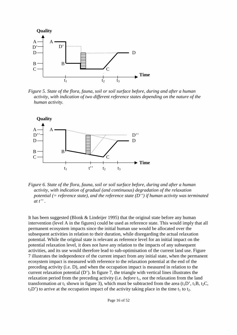
Page 16 of 52

Quality A A D’ D D B B C C Time t1 t2 t3 Figure 5. State of the flora, fauna, soil or soil surface before, during and after a human

activity, with indication of two different reference states depending on the nature of the human activity.

Quality A A D’’ D’’ D D B B C C Time t1 t’’ t2 t3 Figure 6. State of the flora, fauna, soil or soil surface before, during and after a human

activity, with indication of gradual (and continuous) degradation of the relaxation potential (= reference state), and the reference state (D’’) if human activity was terminated at t’’ .

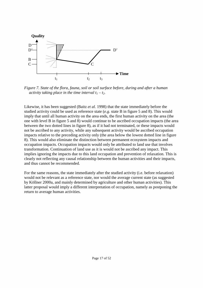
It has been suggested (Blonk & Lindeijer 1995) that the original state before any human intervention (level A in the figures) could be used as reference state. This would imply that all permanent ecosystem impacts since the initial human use would be allocated over the subsequent activities in relation to their duration, while disregarding the actual relaxation potential. While the original state is relevant as reference level for an initial impact on the potential relaxation level, it does not have any relation to the impacts of any subsequent activities, and its use would therefore lead to sub-optimisation of the current land use. Figure 7 illustrates the independence of the current impact from any initial state, when the permanent ecosystem impact is measured with reference to the relaxation potential at the end of the preceding activity (i.e. D), and when the occupation impact is measured in relation to the current relaxation potential (D’). In figure 7, the triangle with vertical lines illustrates the relaxation period from the preceding activity (i.e. before t1, not the relaxation from the land transformation at t1 shown in figure 3), which must be subtracted from the area (t1D’, t1B, t2C, t3D’) to arrive at the occupation impact of the activity taking place in the time t1 to t2.

D’

Page 17 of 52

Quality D D’ D’ B C C Time t1 t2 t3 Figure 7. State of the flora, fauna, soil or soil surface before, during and after a human

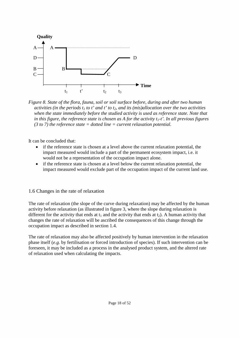
activity taking place in the time interval t1 – t2. Likewise, it has been suggested (Baitz et al. 1998) that the state immediately before the studied activity could be used as reference state (e.g. state B in figure 5 and 8). This would imply that until all human activity on the area ends, the first human activity on the area (the one with level B in figure 5 and 8) would continue to be ascribed occupation impacts (the area between the two dotted lines in figure 8), as if it had not terminated, or these impacts would not be ascribed to any activity, while any subsequent activity would be ascribed occupation impacts relative to the preceding activity only (the area below the lowest dotted line in figure 8). This would also eliminate the distinction between permanent ecosystem impacts and occupation impacts. Occupation impacts would only be attributed to land use that involves transformation. Continuation of land use as it is would not be ascribed any impact. This implies ignoring the impacts due to this land occupation and prevention of relaxation. This is clearly not reflecting any causal relationship between the human activities and their impacts, and thus cannot be recommended. For the same reasons, the state immediately after the studied activity (i.e. before relaxation) would not be relevant as a reference state, nor would the average current state (as suggested by Köllner 2000a, and mainly determined by agriculture and other human activities). This latter proposal would imply a different interpretation of occupation, namely as postponing the return to average human activities.

Page 18 of 52

Quality A A D D B B C C Time t1 t’ t2 t3 Figure 8. State of the flora, fauna, soil or soil surface before, during and after two human

activities (in the periods t1 to t’ and t’ to t2, and its (mis)allocation over the two activities when the state immediately before the studied activity is used as reference state. Note that in this figure, the reference state is chosen as A for the activity t1-t’. In all previous figures (3 to 7) the reference state = dotted line = current relaxation potential.

It can be concluded that:

�� if the reference state is chosen at a level above the current relaxation potential, the impact measured would include a part of the permanent ecosystem impact, i.e. it would not be a representation of the occupation impact alone.

�� if the reference state is chosen at a level below the current relaxation potential, the impact measured would exclude part of the occupation impact of the current land use.

1.6 Changes in the rate of relaxation The rate of relaxation (the slope of the curve during relaxation) may be affected by the human activity before relaxation (as illustrated in figure 3, where the slope during relaxation is different for the activity that ends at t1 and the activity that ends at t2). A human activity that changes the rate of relaxation will be ascribed the consequences of this change through the occupation impact as described in section 1.4. The rate of relaxation may also be affected positively by human intervention in the relaxation phase itself (e.g. by fertilisation or forced introduction of species). If such intervention can be foreseen, it may be included as a process in the analysed product system, and the altered rate of relaxation used when calculating the impacts.

Page 19 of 52

2. Indicators for measuring nature value In order to make the impact assessment operational, it is necessary to find one or more indicators that adequately reflect and quantify the “Quality” on the Y-axes of figures 3 to 8. It follows from these figures that the same indicators should be relevant for both permanent ecosystem impacts (measured in units of quality * area) and occupation impacts (measured in units of quality * area * time). An adequate set of indicators must reflect the key aspects of the impact chains as described in section 1.3.3. Indicators may be defined at several levels of the impact chain (exchange, midpoint or endpoint). Taking a starting point in the areas of protection in figure 2, the following types of indicators may be distinguished: �� Indicators for the biogeochemical substance and energy cycles, being part of the impact

chains for the life-support functions. �� Indicators for the actual or potential productivity of the ecosystems, relating to the

availability of biotic resources, the potential for agriculture, and most of the life-support functions.

�� Indicators for the biodiversity of the ecosystems, relating directly to the endpoint “Biodiversity” under “Resources”, and also being indicators for species composition as a mid-point to other areas of protection.

�� Indicators for the cultural value of the affected sites, in terms of uniqueness of landscapes and archaeological remains.

�� Indicators for migration and dispersal, as one of the midpoints towards altered species composition.

These five types of indicators are dealt with in more detail in the following sections.

2.1 Substance and energy cycles

Altered species composition and population volumes will affect the biogeochemical cycles of substances and energy in many ways. The carbon cycle is of particular interest to the global temperature regulation, as the atmospheric concentration of CO2 and CH4 play a key role in this regulation. An increased atmospheric concentration of these so-called greenhouse gases will decrease the heat loss from the earth through infrared radiation, thus leading to global warming. By photosynthesis, CO2 is taken up by plants, later to be released through respiration and decomposition of organic matter. Although this implies a neutral long-term net effect on the atmospheric concentration of CO2, the temporary storage in organic matter is of a size that

Page 20 of 52

cannot be ignored as sink and source of atmospheric CO2 when assessing the impact of land use on the global temperature regulation. Net primary productivity (NPP, see section 2.2) may be used as an intermediate indicator for the change in fixation and release of CO2 as a result of altered species composition and population volumes. When converted to CO2, the impact on global warming can be calculated from the same models that are used to assess the impact of industrial sources of CO2. However, the dynamics of the modelling and the time horizon of the assessment are of particular importance for CO2 from area sources. Decomposition of organic matter under waterlogged conditions in wetland soils result in release of CH4. Physical changes that affect the size of the waterlogged area or the duration of the waterlogged condition will obviously have a direct impact on the CH4 release. For the waterlogged soils, NPP (see section 2.2) may be used as an intermediate indicator for CH4 release, since decomposition is here proportionally related to NPP. Also for this issue, the ordinary models for global warming can be used to assess the impact. The fixation of nitrogen through soil-living organisms, especially those linked to leguminous plants, is an essential part of the natural supply of nitrogen for plant growth. However, the importance of natural fixation is currently limited, since the global supply of industrial nitrogen-sources is now equivalent in size to the natural fixation, which has had the consequence that it is rather the amount of unwanted nitrogenous substances that is of concern, causing eutrofication (nutrification) both in aquatic and terrestrial environments, and with serious implications for the biodiversity of ecosystems adapted to nitrogen-poor conditions. Thus, compared to other mechanisms, the importance of vegetation-changes on the nitrogen cycle are limited. The concentration of aerosols and dust in the atmosphere is influenced by vegetation, since vegetation reduces wind speeds and surface susceptibility to wind erosion, and at the same time filters the air, thus removing dust from the atmosphere. For most plant micro-nutrients, redistribution through wind is the main natural process for transfer between ecosystems. In the absence of more detailed models and data, the influence of vegetation on atmospheric dust may be estimated by indicators related to vegetation cover, leaf area index, above-ground biomass, or primary productivity (see section 2.2). The same models that are used to assess the impact of industrial sources of dust can be used to assess the impact from a vegetation-induced change in the atmospheric dust concentration. The hydrological cycle is influenced in many ways by the amount and structure of the vegetation as well as by surface characteristics. Vegetation plays a role for water interception, reduction of run-off, and modification of evaporation (increasing evaporation when water is freely available and decreasing evaporation when water is scarce). By changing the albedo and surface roughness, vegetation may also influence the distribution of precipitation. If albedo increases, evaporation decreases and precipitation markedly decreases. This effect may be self-amplifying, since reductions in vegetation typically increase the albedo and decrease surface roughness. The surface characteristics are important for direct evaporation as well as for the partitioning of precipitation between run-off and infiltration. Many empirically based models exist for parts of the hydrological cycle on local scales (and dependent on the locally available input data), but models based on proven, generalised relationships on regional and global level are still under development. For a survey of current research, see http://www. gewex.com/. It appears that globally applicable indicators are not yet available for the impact

Page 21 of 52

of vegetation and soil properties on the hydrological cycle. Until more universally applicable models become available, the influence of vegetation on water inception, reduction of run-off, and stabilization of evaporation, may be assumed linearly related to the amount of vegetation, e.g. expressed in terms of above-ground biomass or primary productivity, which may therefore be used as a preliminary rough indicator (see section 2.2). The influence of the vegetation on the energy balance takes place both indirectly, via the hydrological balance just described, and directly through the albedo. As for the issues above, the influence of vegetation on the energy balance may - in the absence of more detailed models and data - be assumed linearly related to above-ground biomass or primary productivity (se section 2.2).

2.2 Ecosystem productivity In terrestrial ecosystems, the availability of biotic resources is - on a very general level - related to their productivity potential. While it may be possible in specific situations to model the direct influence of altered species composition and population volumes on specific species that supply goods and services for human use, the typical level of information will only allow the use of general indicators for productivity. The productivity potential is an even more directly appropriate indicator for the potential for agriculture. And as already indicated in the preceding section, ecosystem productivity can be used as a more or less satisfying indicator for many biogeochemical substance and energy cycles that are part of the impact chains for many life-support functions. In addition to the mechanisms described in the preceding section, primary productivity is linked to further important mid- or end-points of life-support functions, namely: �� Decomposition, which plays an important role for nutrient availability and topsoil

formation, is determined mainly by turnover of organic matter, as measured by net primary productivity.

�� Dislocation of substances by and through organisms, closely related to the above, but also including the transport of nutrients between ecosystems by and in migrating species. Again, in absence of more specific indicators, the net primary productivity appears to be a reasonable proxy indicator.

�� Topsoil formation and preservation. Along with weathering, organic matter plays a key role in topsoil formation, and vegetation cover plays a key role in topsoil preservation. Thus, net primary productivity is a reasonable indicator for both mechanisms.

In conclusion, change in net primary productivity (NPP), which is defined as the net carbon uptake of the ecosystem (fixation through photosynthesis minus losses through respiration) over time, appears to be a reasonable mid-point indicator for the impact of altered species composition and population volumes on biotic resources, potential for agriculture, and life-support functions of natural systems. This may be substituted and/or amended by other indicators, such as above-ground biomass, when relevant data and models become available for the described processes.

Page 22 of 52

As an indicator for impacts from land use on life-support, Blonk & Lindeijer (1995) and Lindeijer et al. (1998) have suggested free net primary productivity (fNPP), i.e. NPP minus the amount of carbon sequestered for human use. However, they view this as an indicator for “nature development space”, i.e. the amount of biomass nature can apply freely for its own development. In this sense, it may be a better indicator for impacts on biodiversity (see section 2.3) than for impacts on life-support, since most life-support functions listed in section 1.3 are related to the full NPP, i.e. the overall turnover of biomass, disregarding whether human use is a part of this turnover. The impact of ecosystems on the carbon cycle, nitrogen fixation, the concentration of atmospheric dust, the hydrological cycle, and the energy balance are all closer related to NPP than to fNPP, since it is the productivity and functioning of the ecosystem which is essential, not the route of utilisation of the products (by humans or within the ecosystem itself). A possible exception to this is decomposition and the formation of topsoil, which obviously depend on the organic matter left in the ecosystem. However, the human removal of organic matter and nutrients is separately modelled as a substance flow impact of the specific land use (see section 1.2) which may then subtract from the positive effects related to NPP. The use of NPP as an indicator for “nature value” may appear counter-intuitive when confronted with the fact that man-made ecosystems may have a higher NPP than natural ecosystems on the same latitude, partly due to the higher proportion of young individuals with a high productivity, partly due to fertilisation, irrigation and other management practices. This implies that managed ecosystems can have a higher “nature value” than natural systems. This is, however, not surprising when considering that the “nature value” we seek to capture with the indicator NPP is mainly related to the gross influence of vegetation on climate and substance flows, which is clearly related to vegetation turnover, which is exactly promoted in managed ecosystems. Nevertheless, it is possible to criticize this choice of indicator for not adequately including the effects of harvesting. If a managed ecosystem is repeatedly harvested by removing the majority of above-ground biomass, the NPP may be kept high although important life-support functions may be endangered in the periods immediately after harvest and until an adequate plant cover is re-established. This is especially true for those impact chains that involve mid-points or mechanisms related more to vegetation cover or structure than to biomass turnover, such as the influence of vegetation on wind speed, interception of precipitation and dust, evapotranspiration, and albedo. When possible, it may therefore be appropriate to combine NPP with other indicators that better reflect vegetation cover and structure. Another option may be to make the NPP measure more dynamic and assign more importance to particularly low levels of NPP even when these low levels appear only at shorter intervals that are not reflected adequately in the annual average NPP.

2.3 Biodiversity Biodiversity may be seen both as an indicator for the species composition of ecosystems, which is a mid-point for many impact chains (see figure 2), and as an endpoint in itself under the area of protection “Resources”. Biodiversity is a term covering genetic diversity, species diversity, and ecosystem diversity. The three levels are interrelated in the sense that the preservation of diversity at the higher levels requires genetic diversity, and the maintenance of genetic diversity often requires in vivo conditions of species, which again requires the

Page 23 of 52

existence of the ecosystems. Since the area of protection “life-support functions” includes the key, irreversible aspects of ecosystem maintenance, it is reasonable to regard genetic diversity as the remaining irreversible aspect, i.e. the resource aspect, of biodiversity. In practice, nevertheless, data are most easily available for species diversity, and especially for vascular plant species. Thus, vascular plant diversity is an obvious proxy upon which to base any practical biodiversity indicator. Vascular plants also play a key role in ecosystem functions, and vascular plant diversity appears to be reasonably well correlated with terrestrial species diversity in general (Rosenzweig 1995, Barthlott et al. 1996). This proxy may either be further validated by specific investigations, or may later be modified to include also other species. In the context of LCA, a biodiversity indicator based exclusively on vascular plant species richness2 was developed by Lindeijer et al. (1998) and Köllner (2000a & b), the latter also applied in a modified draft form in the Eco-Indicator 99 (Goedkoop & Spriensma 1999). These indicators express loss of vascular plant species richness in relative terms, through dividing by a local reference state, in accordance with the 1992 Rio de Janeiro Convention on Biological Diversity, which discourages absolute scores for species diversity, since a reduction of say 5 species out of a total of 20 species in the Northern countries is considered worse than a reduction of 5 species out of a total of 200 species in the tropics. Köllner chose average actual or historical levels of species diversity as reference states, while Lindeijer et al. use the maximum actual species diversity. The latter is in better accordance with the rationale presented in section 1.5. Also in the context of LCA, a biodiversity indicator based on the absolute number of rare species was proposed by Müller-Wenk (1998). The basis for this proposal is an assumption regarding the relationship between the number of rare species and the area of intensively used land, combined with data on rare species from Switzerland and Germany. The approach is noteworthy as an attempt to quantify the marginal impact of land use on biodiversity. Nevertheless, the current applicability on a global level is limited, due to lack of data. In the early work from the LCAGAPS sub-project on land use (Schmidt 1997), we suggested to base the biodiversity assessment on the concept of relative scarcity on each ecosystem level (biome, biotope, habitat, species). In vivo species conservation is completely dependent on the conservation of the ecosystems. Thus, ecosystem scarcity is regarded as an essential part of a biodiversity indicator. To use factors for each ecosystem level is in line with the concepts of the 1992 Rio de Janeiro Convention on Biological Diversity. It was also suggested that the scarcity indicator could be supplemented by a vulnerability factor to take into account that two equally scarce ecosystems may not be equally vulnerable. Also Cowell (1998) proposed a semi-quantitative indicator system for global biodiversity impacts of land use in the context of LCA, with four factors expressing relative ecosystem scarcity (through the relative area of such ecosystems), relative number of rare species (relative to a postulated maximum), relative species richness (relative to a maximum differentiated in relation to latitude), and relative number of individuals (expressed by the proxy indicator NPP relative to a maximum NPP per ecosystem type).

2 We use “species richness” to signify “number of species per area”. In technical literature, both this term and the term “species density” are used in this meaning, but unfortunately both terms are also found to be applied with different meanings.

Page 24 of 52

As part of the LCAGAPS sub-project on land use, the results of which is presented with the present report, we have developed the above concepts of scarcity and vulnerability further. As a basis, we use the most simple measure available for biodiversity: �� Species richness (SR) of the ecosystem. This basic measure is then modified by two factors at ecosystem level: �� Inherent ecosystem scarcity (ES), expressed as the inverse of the potential area (1/Apot) that

could be occupied by the ecosystem if left undisturbed by human activities. �� Ecosystem vulnerability (EV), indicating the relative number of species affected by a

change in the ecosystem area, as expressed by the species-area relationship. When combining several factors expressing different aspects of biodiversity, these must be related to one another in order to arrive at a consistent indicator system that can be applied on various levels of detail once data is available. Therefore, each factor should have a conceptual link with the others. We link the three factors by multiplication, which forces us to relate each factor to one another, and to determine the weights of each factor. In a multiplication, the inherent weight of each factor is determined by the range of its possible values. To compare these inherent ranges, we therefore normalise each factor so that the lowest scoring ecosystem is unity, and analyse the resulting quality indicator for bias. The development of this biodiversity indicator is described in more detail in the following sub-sections.

2.3.1 Species richness (SR) The most simple measure for biodiversity is species richness (SR), i.e. number of species per area. Data on the largest groups (about 160’000 micro-organism species, 130’000 soil macrofauna species, 31’000 lower plant species and 15’000 nematode species) is largely lacking (Groombridge, 1992). Higher – vascular - plants (about 263’000), fishes (nearly 22’000 described) and vertebrates (43’000 species) offer the best chance. Of these, vascular plant species richness is proposed as reasonable indicator for species richness in general, since there are no other species group for which global data are available to a reasonable extent, and since vascular plant species are generally regarded as predictive for the diversity of other species (Rosenzweig 1995, Barthlott et al. 1996). Even when vascular plant species are accepted as a reasonable indicator for other species, a refinement could be to correct this proxy for actual values whenever available. To normalise SR, so that the value of the lowest scoring ecosystem is unity, we must divide by the minimum vascular plant species richness (SRmin), arriving at:

nSR = SR/SRmin (1) At the biome level, SRmin is set to 100 species per 10000 km2 (found in deserts, tundra and on ice caps - see table 5). The setting of the minimum species richness determines the inherent weight of this factor, since this determines the range of its possible values (1 to >90, see table 1 in section 2.3.4).

Page 25 of 52

It may be argued that the biodiversity indicator should rather reflect the number of indigenous species (as opposed to non-indigenous/neophytes, intentionally or accidentally introduced by man) and endemic species (species not found elsewhere) than the overall species number (Barthlott et al. 1999, Williams et al. 1994, Kier & Barthlott in press). With large numbers of non-indigenous species, the overall species richness may well be high, while indigenous and endemic species are still endangered, e.g. by invasive alien species. When improved data become available for indigenous and endemic species at a global level, these concerns may be included in the species richness (SR) factor. Also from a conservationist viewpoint, those species would be crucial that are endangered or rare. The number of rare species would then be taken as an indicator for the ecosystem value. A potential refinement in line with this would be to determine the rareness of species (and possibly indirectly ecosystems) based on their mutual genetic distance (phylogenetic diversity). This would directly address the genetic part of the endpoint “biodiversity.” Another possible refinement is to amend with diversity indicators determined by ecologists, such as key species (performing key functions in the ecosystem), or other indicators (see examples for Northern forest ecosystems in Hansson 2000). However, a requirement for a refinement would be that the resulting indicator should be unbiased across ecosystems. As a central measure for biodiversity, the choice of species richness is in line with common sense understanding of biodiversity (“more species is better”), but may be seen as conflicting with the 1992 Rio de Janeiro Convention on Biological Diversity or national policies on biodiversity, because also species-poor ecosystems, such as heathlands and moors, are considered valuable and contributing to ecosystem diversity in themselves. The adjustment factors described in sections 2.3.2 and 2.3.3, aim to some extent to overcome this conflict.

2.3.2 Inherent ecosystem scarcity (ES) The smaller the area in which an ecosystem is viable (due to its requirement for a particular and possibly rare geophysical condition), the more scarce it (and its species) can be said to be, even in a natural situation without human impacts. Thus, the same area should be assigned a higher value in an ecosystem with a small potential area than in an ecosystem with a larger potential area. This implies that the Inherent Ecosystem Scarcity (ES) can be expressed by a reverse relationship with the potential area of the ecosystem (Apot), resulting in the following formula:

ES = 1 / Apot (2)

Currently, data for Apot are globally available at the biome level (see section 3.3). When data become available at lower ecosystem levels, the ES factor can be redefined to include ecosystem scarcity at these lower levels (following the suggestion of Schmidt 1997), to take into account that these factors may well be different between biotopes and between habitats. Prentice (pers. comm.) indicates that data are available for the development of such factors at least at the biotope level. To normalise ES, so that the value of the lowest scoring ecosystem is unity, we must multiply by the area of largest potential ecosystem area (Apot,max), arriving at:

Page 26 of 52

nES = Apot,max / Apot (3) At the biome level, Apot,max is boreal forests with the area 25*106 km2 (see table 5 in section 3.3). The setting of the largest and the smallest potential ecosystem area determine the inherent weight of nES, since this determines the range of its possible values (1 to 5.4, see table 1 in section 2.3.4).

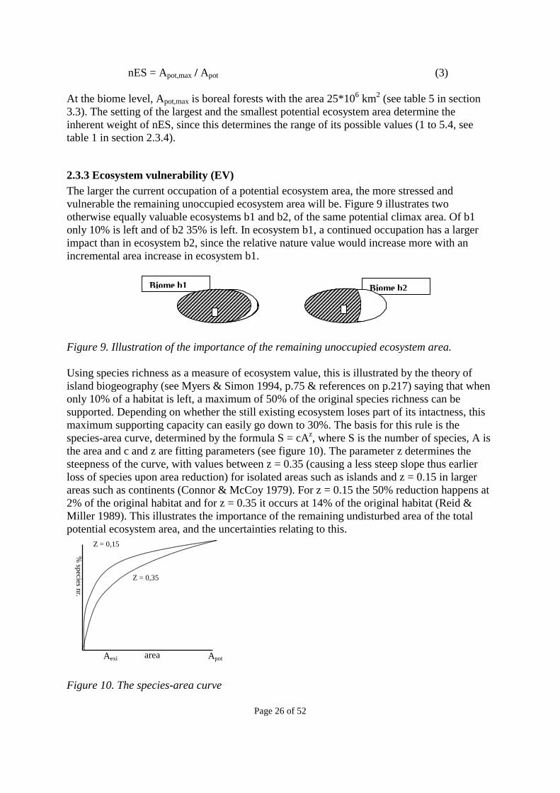
2.3.3 Ecosystem vulnerability (EV) The larger the current occupation of a potential ecosystem area, the more stressed and vulnerable the remaining unoccupied ecosystem area will be. Figure 9 illustrates two otherwise equally valuable ecosystems b1 and b2, of the same potential climax area. Of b1 only 10% is left and of b2 35% is left. In ecosystem b1, a continued occupation has a larger impact than in ecosystem b2, since the relative nature value would increase more with an incremental area increase in ecosystem b1.

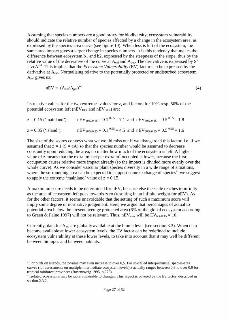
Figure 9. Illustration of the importance of the remaining unoccupied ecosystem area. Using species richness as a measure of ecosystem value, this is illustrated by the theory of island biogeography (see Myers & Simon 1994, p.75 & references on p.217) saying that when only 10% of a habitat is left, a maximum of 50% of the original species richness can be supported. Depending on whether the still existing ecosystem loses part of its intactness, this maximum supporting capacity can easily go down to 30%. The basis for this rule is the species-area curve, determined by the formula S = cAz, where S is the number of species, A is the area and c and z are fitting parameters (see figure 10). The parameter z determines the steepness of the curve, with values between z = 0.35 (causing a less steep slope thus earlier loss of species upon area reduction) for isolated areas such as islands and z = 0.15 in larger areas such as continents (Connor & McCoy 1979). For z = 0.15 the 50% reduction happens at 2% of the original habitat and for z = 0.35 it occurs at 14% of the original habitat (Reid & Miller 1989). This illustrates the importance of the remaining undisturbed area of the total potential ecosystem area, and the uncertainties relating to this.

Figure 10. The species-area curve

Aexi Apot area

% sp

ecies nr.

Z = 0,35

Z = 0,15

Biome b2Biome b1

Page 27 of 52

Assuming that species numbers are a good proxy for biodiversity, ecosystem vulnerability should indicate the relative number of species affected by a change in the ecosystem area, as expressed by the species-area curve (see figure 10). When less is left of the ecosystem, the same area impact gives a larger change in species numbers. It is this tendency that makes the difference between ecosystem b1 and b2, expressed by the steepness of the slope, thus by the relative value of the derivative of the curve at Aexi and Apot. The derivative is expressed by S’ = zcAz-1. This implies that the Ecosystem Vulnerability (EV) factor can be expressed by the derivative at Aexi. Normalising relative to the potentially protected or undisturbed ecosystem Apot gives us:

nEV = (Aexi/Apot)z-1 (4)

Its relative values for the two extreme3 values for z, and factors for 10% resp. 50% of the potential ecosystem left (nEV10% and nEV50%) are: z = 0.15 (‘mainland’): nEV10%/0.15 = 0.1-0.85 = 7.1 and nEV50%/0.15 = 0.5-0.85 = 1.8 z = 0.35 (‘island’): nEV10%/0.35 = 0.1-0.65 = 4.5 and nEV50%/0.35 = 0.5-0.65 = 1.6 The size of the scores conveys what we would miss out if we disregarded this factor, i.e. if we assumed that z = 1 (S = cA) so that the species number would be assumed to decrease constantly upon reducing the area, no matter how much of the ecosystem is left. A higher value of z means that the extra impact per extra m2 occupied is lower, because the first occupation causes relative more impact already (so the impact is divided more evenly over the whole curve). As we consider vascular plant species diversity in a wide range of situations, where the surrounding area can be expected to support some exchange of species4, we suggest to apply the extreme ‘mainland’ value of z = 0.15. A maximum score needs to be determined for nEV, because else the scale reaches to infinity as the area of ecosystem left goes towards zero (resulting in an infinite weight for nEV). As for the other factors, it seems unavoidable that the setting of such a maximum score will imply some degree of normative judgement. Here, we argue that percentages of actual to potential area below the present average protected area (6% of the global ecosystem according to Green & Paine 1997) will not be relevant. Thus, nEVmax will be EV6%/0.15 = 10. Currently, data for Aexi are globally available at the biome level (see section 3.3). When data become available at lower ecosystem levels, the EV factor can be redefined to include ecosystem vulnerability at these lower levels, to take into account that it may well be different between biotopes and between habitats.

3 For birds on islands, the z-value may even increase to over 0,5. For so-called interprovincial species-area curves (for assessments on multiple intermediate ecosystem levels) z actually ranges between 0,6 to over 0,9 for tropical rainforest provinces (Rosenzweig 1995, p.276). 4 Isolated ecosystems may be more vulnerable to changes. This aspect is covered by the ES factor, described in section 2.3.2.

Page 28 of 52

2.3.4 Combining the biodiversity factors Now, the three factors nSR, nES, and nEV are combined through multiplication to arrive at the biodiversity indicator adequately reflecting and quantifying the Quality (Q) on the Y-axes of figures 3 to 8. This forces us to relate each factor to one another, and to determine the weights (a, b, and c) of each factor:

Qbiodiversity = nSRa * nESb * nEVc (5)

If we set a = b = c = 1, the weight of each factor is determined by the inherent range in its values. The preliminary maximum ranges and main choices therein are summarized in table 1. Table 1. Overview of factor ranges (see also table 5 in section 3.3) Factor Preliminary range Main choices Species Richness 1 – 90 Including all species or only indigenous, endemic

or rare species – here all species. The expression for species richness: SR, the

Fischer log form, or the Arrhenius exponent form – here the plain SR.

The minimum value of SR: 100/10000km2. Ecosystem Scarcity

1 – 5.4 The level at which ecosystems are assessed: biome, biotope, habitat – here biome only.

The ecosystem classification system used – here Biome 2.

Ecosystem Vulnerability

1 – 10

The maximum value of EV, determined by z and the % of ecosystem currently protected – here 0.15 and 6%, respectively.

A more detailed classification, for instance based on vegetation types (such as the Biome 3 model), may reduce the range in some of the factors considerably. Nevertheless, the area occupied will still dominate the whole impact assessment, as its range can in practice be a factor 10'000 for cases comparing renewable and non-renewable materials. This dominance of the area occupied is inherent to the focus on occupation. For permanent ecosystem change, area becomes less important and the scarcity aspect more important. The total weight of all proposed factors is equal to their multiplied range. No arguments have been found to warrant the setting the weights a, b or c to any other value than 1, which means that we can simplify formula 5 to: Qbiodiversity = nSR * nES * nEV (6) or, for the purposes of relating to the basic data: Qbiodiversity = (SR / SRmin) * (Apot,max / Apot) * (Aexi / Apot)

-0.85 (7)

Page 29 of 52

Note that Qbiodiversity, and especially the factor nEV, may change over time, which means that the scale of the Y-axis in figures 3 to 8 is not stable over longer time periods - not as a result of the currently studied land use, but due to changes in the human land use in general (Aexi), or even due to changes in natural conditions (Apot). This implies that the figures 3 to 8 must be understood to illustrate marginal changes, i.e. changes that are small compared to the overall size of the ecosystems. In parallel, the data in section 3 are applicable only for marginal changes.

2.4 Cultural value In contrast to the impacts and indicators discussed above, unique landscapes and unique archaeological sites under the area of protection “Resources” do not have a value outside the context of human culture. While unique landscapes may indeed be natural, they may as well be man-made, and certainly archaeological sites cannot be measured in terms of “nature value.” This implies that the concepts outlined in sections 1.4 to 1.6 and illustrated in figures 3 to 8 are not appropriate for these culturally dependent areas of protection. The impacts on unique landscapes and unique archaeological sites are not related to occupation. Indeed, the conservation of landscapes and archaeological sites may actually require human occupation, since the relaxation into a natural state may lead to their disruption or disappearance. Nor are the impacts related to any relaxation level, since unique landscapes and unique archaeological sites per definition cannot be recovered. The impacts on unique landscapes and unique archaeological sites are fundamentally related to transformation itself, whether this transformation is one from a natural state into human use, from one human use to another, or a relaxation from human use. Thus, for these impacts, the reference level (cf. the discussion in section 1.5) is indeed the state immediately before the studied activity. Any change from this previous state may imply an impact. Exactly because of their uniqueness, the value of unique landscapes and unique archaeological sites cannot be determined in terms of a general indicator, but must be treated on a case-by-case basis. However, an indicator may be developed for disruption of unknown archaeological sites (i.e. possibly but not necessarily unique), since this can be related to increases in ploughing depth, introduction of deep-rooted plants, and other activities that disturb or remove soil layers that were previously undisturbed. Thus, an indicator may be based on the thickness of soil layer disturbed. This indicator should be multiplied by the area, and weighted by a factor determined by archaeologists and historians, expressing the probability of occurrence of archaeological remains in different area types (and soil depths). Predictive models for this purpose are in development (see e.g. Dalla Bona 1994). As for ecosystems, the possibility for a meaningful classification of area types depends also on the ability of the life cycle inventory to identify the location of specific activities within such classes (see section 4.1).

Page 30 of 52

2.5 Migration and dispersal

The subdivision of habitats or creation of barriers by cutting corridors, typically by draining or by construction of larger roads or barrages in streams, will impact biotic migration and dispersal patterns. In some species, migration is an essential part of the life cycle of individuals, as known especially from birds and larger sea-living animals. But also smaller movements may be of importance, such as animals in the mating season roaming in search of a partner. Dispersal refers to the broader issue of gene flow at population level. However, dispersal capabilities of single organisms are increasingly considered to be crucial for the survival probability of threatened species. For both migration and dispersal, indicators related to landscape structure are of interest. One such indicator is connectivity, which is the degree to which a landscape facilitates or impedes movement of organisms among resource patches. However, measurement of connectivity is not uncontroversial (Tischendorf & Fahrig 2000a & b). Although the role of fragmentation increases in landscapes with low habitat coverage, it appears that the amount and quality of habitats in general play a larger role for landscape connectivity than landscape fragmentation. This appears to be true, even for the larger scale of wetland areas as stopover sites for migratory birds, where the quality of wetland sites (i.e. food availability) was found to be substantially more important than the spacing of sites along the migratory pathway (Farmer and Wiens in press). This suggests that the general indicators for productivity and biodiversity may to some extent cover the concern for connectivity. We therefore refrain from development of additional indicators for migration and dispersal. A possibly more serious problem is the reverse: namely the increase in dispersal of invasive species, alien to the local ecosystems. This may happen through creation of new corridors or dispersal vectors, or through intentional introductions. This may be classified as a physical change to flora and fauna, with direct impacts on altered species composition (arrow 1 in figure 2). As mentioned in section 2.3, this may be reflected in a refined biodiversity indicator, when models are developed that allow data on indigenous and endemic species to be distinguished from the overall species number.

Page 31 of 52

3. Data and maps For the practical application of the different indicators discussed in chapter 2, data availability is a crucial issue. We have focussed on presenting data for a few of the most central indicators, while for other indicators we limit ourselves to describe the availability of data in general terms, either because these indicators have been treated extensively elsewhere, or because a treatment here would be meaningless in the light of the rapid developments in the particular fields.

3.1 Data for substance and energy cycles

Carbon dioxide sequestration can be calculated directly from NPP values (which are either reported as carbon or easy to convert from biomass to carbon). For land transformations, the carbon in live vegetation is of interest. Data can be found in Olson et al. (1985), or see table 2. According to the IPCC methodology, methane emission from rice fields is estimated at an average of 20g/yr/m2. The ratio of methane emission to net primary productivity can be estimated to an average 3% on a carbon-to-carbon basis, based on field measurements in rice fields (Huang et al. 1996). See also Matthews (1993). Atmospheric dust from unvegetated areas is mainly related to recently disturbed soils. Data can be found in Gillette (1978) and Tegen & Fung (1994). Albedo for vegetated areas are typically 10-20%, while for unvegetated areas, the albedo is 20-45% depending on clay and organic matter content (see e.g. Matthews 1983).

3.2 Data for ecosystem productivity Data for net primary productivity are given in table 2. Dobben et al. (1998) provide a world map of net primary productivity per physiotype. Table 3 provides a rough summary of this map relating NPP to latitude and altitude. Figure 11 displays a similar map, based entirely on satellite imagery by the Laboratory for Global Remote Sensing Studies (http://www.geog.umd.edu/glopem/), see also Prince & Goward (1995).

Page 32 of 52

Table 2. Annual net primary productivity (NPP), and carbon content in plants and soil (0-1 metre) in broadly categorized terrestrial ecosystems (from Amthor et al. 1998)

Ecosystem NPP Plant C Soil C gC/m2/

year g/m2 g/m2

Forest, tropical 925 16500 8300 Forest, temperate and plantation 670 12270 12000 Forest, Boreal 355 2445 15000 Woodland, temperate 700 8000 12000 Chaparral 360 3200 12000 Savanna, tropical 790 2930 11700 Grassland, temperate 350 720 23600 Tundra, arctic and alpine 105 630 12750 Desert and semidesert scrub 67 330 8000 Desert, extreme 11 35 2500 Lake and stream 200 10 - Wetland 1180 4300 72000 Cultivated and permanent crop 425 200 7900 Human area 100 500 5000 AVERAGE 391 3220 13640

Table 3. Estimates of NPP (gC/m2/year) for dry physiotopes (table from Dobben et al. 1998, recalculated assuming 45% C in biomass).

Altitude: Latitude:

0 - 1000

1000-3000

>3000

80 <=50 0 0

60 360 140 0 40 540 360 90 30 <=50 <=50 <=50 20 720 360 140 0 990 540 180

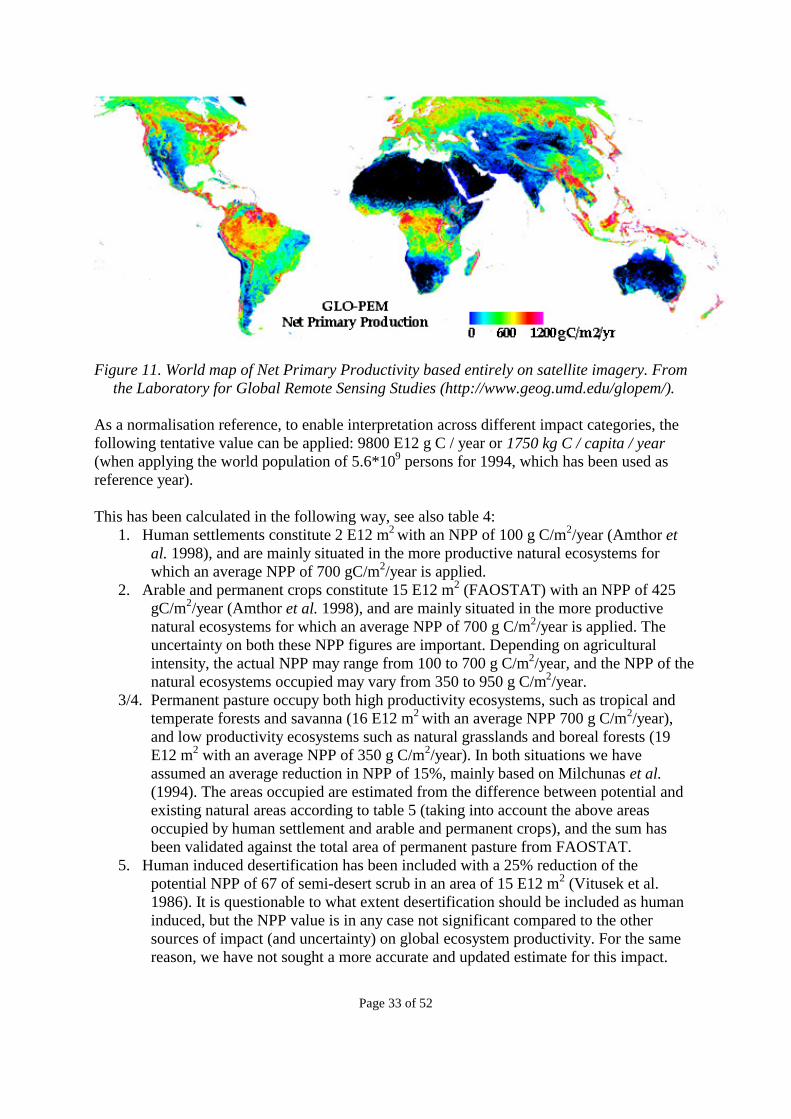
Page 33 of 52

Figure 11. World map of Net Primary Productivity based entirely on satellite imagery. From

the Laboratory for Global Remote Sensing Studies (http://www.geog.umd.edu/glopem/). As a normalisation reference, to enable interpretation across different impact categories, the following tentative value can be applied: 9800 E12 g C / year or 1750 kg C / capita / year (when applying the world population of 5.6*109 persons for 1994, which has been used as reference year). This has been calculated in the following way, see also table 4:

1. Human settlements constitute 2 E12 m2 with an NPP of 100 g C/m2/year (Amthor et al. 1998), and are mainly situated in the more productive natural ecosystems for which an average NPP of 700 gC/m2/year is applied.

2. Arable and permanent crops constitute 15 E12 m2 (FAOSTAT) with an NPP of 425 gC/m2/year (Amthor et al. 1998), and are mainly situated in the more productive natural ecosystems for which an average NPP of 700 g C/m2/year is applied. The uncertainty on both these NPP figures are important. Depending on agricultural intensity, the actual NPP may range from 100 to 700 g C/m2/year, and the NPP of the natural ecosystems occupied may vary from 350 to 950 g C/m2/year.

3/4. Permanent pasture occupy both high productivity ecosystems, such as tropical and temperate forests and savanna (16 E12 m2 with an average NPP 700 g C/m2/year), and low productivity ecosystems such as natural grasslands and boreal forests (19 E12 m2 with an average NPP of 350 g C/m2/year). In both situations we have assumed an average reduction in NPP of 15%, mainly based on Milchunas et al. (1994). The areas occupied are estimated from the difference between potential and existing natural areas according to table 5 (taking into account the above areas occupied by human settlement and arable and permanent crops), and the sum has been validated against the total area of permanent pasture from FAOSTAT.

5. Human induced desertification has been included with a 25% reduction of the potential NPP of 67 of semi-desert scrub in an area of 15 E12 m2 (Vitusek et al. 1986). It is questionable to what extent desertification should be included as human induced, but the NPP value is in any case not significant compared to the other sources of impact (and uncertainty) on global ecosystem productivity. For the same reason, we have not sought a more accurate and updated estimate for this impact.

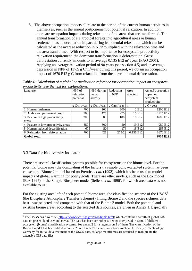
Page 34 of 52

6. The above occupation impacts all relate to the period of the current human activities in themselves, seen as the annual postponement of potential relaxation. In addition, there are occupation impacts during relaxation of the areas that are transformed. The annual transformation of e.g. tropical forests into agricultural areas or human settlement has an occupation impact during its potential relaxation, which can be calculated as the average reduction in NPP multiplied with the relaxation time and the area transformed. With respect to its importance for ecosystem productivity relaxation requirement, the dominant transformation is deforestation. Gross deforestation currently amounts to an average 0.135 E12 m2 /year (FAO 2001). Applying an average relaxation period of 90 years (see section 4.5) and an average depression in NPP of 137.5 g C/m2/year during this period, we obtain an occupation impact of 1670 E12 g C from relaxation from the current annual deforestation.

Table 4. Calculation of a global normalisation reference for occupation impact on ecosystem productivity. See the text for explanations. Land use NPP of

relaxation potential

NPP during human activity

Reduction in NPP

Area affected

Annual occupation impact on ecosystem productivity

g C/m2/year g C/m2/year g C/m2/year m2 g C / year 1. Human settlement 700 100 600 2 E12 1200 E12 2. Arable and permanent crops 700 425 275 15 E12 4125 E12 3. Pasture in high productivity areas

700 600 100 16 E12 1600 E12

4. Pasture in low productivity areas 350 300 50 19 E12 950 E12 5. Human induced desertification 67 50 17 15 E12 255 E12 6. Relaxation from deforestation 700 425 275/2 0.135 E12 1670 E12 Global total 9800 E12

3.3 Data for biodiversity indicators

There are several classification systems possible for ecosystems on the biome level. For the potential biome area (the dominating of the factors), a simple policy-oriented system has been chosen: the Biome 2 model based on Prentice et al. (1992), which has been used to model impacts of global warming for policy goals. There are other models, such as the Box model (Box 1995) or the Simple Biosphere model (Sellers et al. 1996), for which area data was not available to us. For the existing area left of each potential biome area, the classification scheme of the USGS5 (the Biosphere Atmosphere Transfer Scheme) - fitting Biome 2 and the species richness data best - was selected, and compared with that of the Biome 2 model. Both the potential and existing biome areas, according to the selected data sources, are given in Annex 1. Especially

5 The USGS has a website (http://edcwww.cr.usgs.gov/eros-home.html) which contains a wealth of global GIS data on present land use/land cover. The data has been (or rather is being) interpreted in terms of different ecosystem (biome) classification systems. See annex 2 for a legenda on 5 of them. The classification of the Biome I model has been added to annex 2. We thank Christian Bauer from Aachen University of Technology, Germany for initial data treatment of the USGS data, as large mainframes are required to manipulate the extensive GIS data files.

Page 35 of 52

the difference in agriculture land cover between BATS and Biome 2 is disturbing. The data from BATS seem erroneous, as FAO gives a global agriculture area of 49*106 km2 for 1998 and of 46*106 km2 for 1970. Thus, in table 5, we have used the data from the Biome 2 model to calculate Qbiodiversity. Rough values for the species richness (SR) per biome are taken from Barthlott et al. (1996), a first version of the map in figure 12. These initially collected data may be somewhat erroneous. The two sources for existing land use (BATS and Biome 2) including different % of contributions from each type illustrates the uncertainty range of these data. Clustering of biomes may also be under discussion. This clustering may determine the values for Apot,max and SRmin. We for instance chose boreal forest for Apot,max because the clustering of all grasslands is very different for different classifications and may include very different climate zones, whereas boreal forest seems a more coherent biome class. Thus, uncertainty may be considered high and may be above 50%. However, once a consistent classification scheme is chosen, mainly model uncertainties remain. Depending on the credibility of the model, this may be considered a larger or a minor problem. The data uncertainty on the global level may then be reduced to below 50%. For the present report, these data do give an impression of what the range in the various factors may be (see the overview in table 1). Data collection on a more detailed level has not yet been attempted. An attempt to use Biome 3 may be worthwhile. However, whether all required data would still be available in a consistent manner on this level of resolution is unclear. The ecosystem data will be in terms of vegetation types, and biodiversity data should be available on that level too. Also, more regional scarcity prioritisation schemes may be valid, but in a global approach such as LCA, may lead to serious credibility problems and subsequent data use limitations.

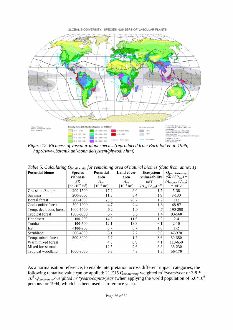
Page 36 of 52

Figure 12. Richness of vascular plant species (reproduced from Barthlott et al. 1996;

http://www.botanik.uni-bonn.de/system/phytodiv.htm) Table 5. Calculating Qbiodiversity for remaining area of natural biomes (data from annex 1) Potential biome Species

richness SR

[no./109 m2]

Potential area Apot

[1012 m2]

Land cover area Aexi

[1012 m2]

Ecosystem vulnerability

nEV = (Aexi / Apot)

-0.85

Qpot, biodiversity

(SR / SRmin) * (Apot,max / Apot)

* nEV Grassland/Steppe 200-1500 17.2 9.0 1.7 5-38 Savanna 200-3000 11.5 5.4 1.9 8-130 Boreal forest 200-1000 25.3 20.7 1.2 212 Cool conifer forest 500-1000 4.7 2.4 1.8 48-97 Temp. deciduous forest 1000-1500 6.2 1.0 4.7 190-290 Tropical forest 1500-9000 5.7 3.8 1.4 93-560 Hot desert 100-200 14.2 11.6 1.2 2-4 Tundra 100-500 12.1 13.3 ~ 1 2-10 Ice <100-200 6.7 6.7 1.0 1-2 Scrubland 500-4000 8.1 2.2 3.0 47-370 Temp. mixed forest Warm mixed forest Mixed forest total

500-3000 7.7 4.8

12.5

1.7 0.9 2.6

3.6 4.1 3.8

59-350 110-650 38-230

Tropical woodland 1000-3000 6.8 4.3 1.5 56-170 As a normalisation reference, to enable interpretation across different impact categories, the following tentative value can be applied: 21 E15 Qbiodiversity-weighted m2*years/year or 3.8 * 106 Qbiodiversity-weighted m2*years/capita/year (when applying the world population of 5.6*109 persons for 1994, which has been used as reference year).

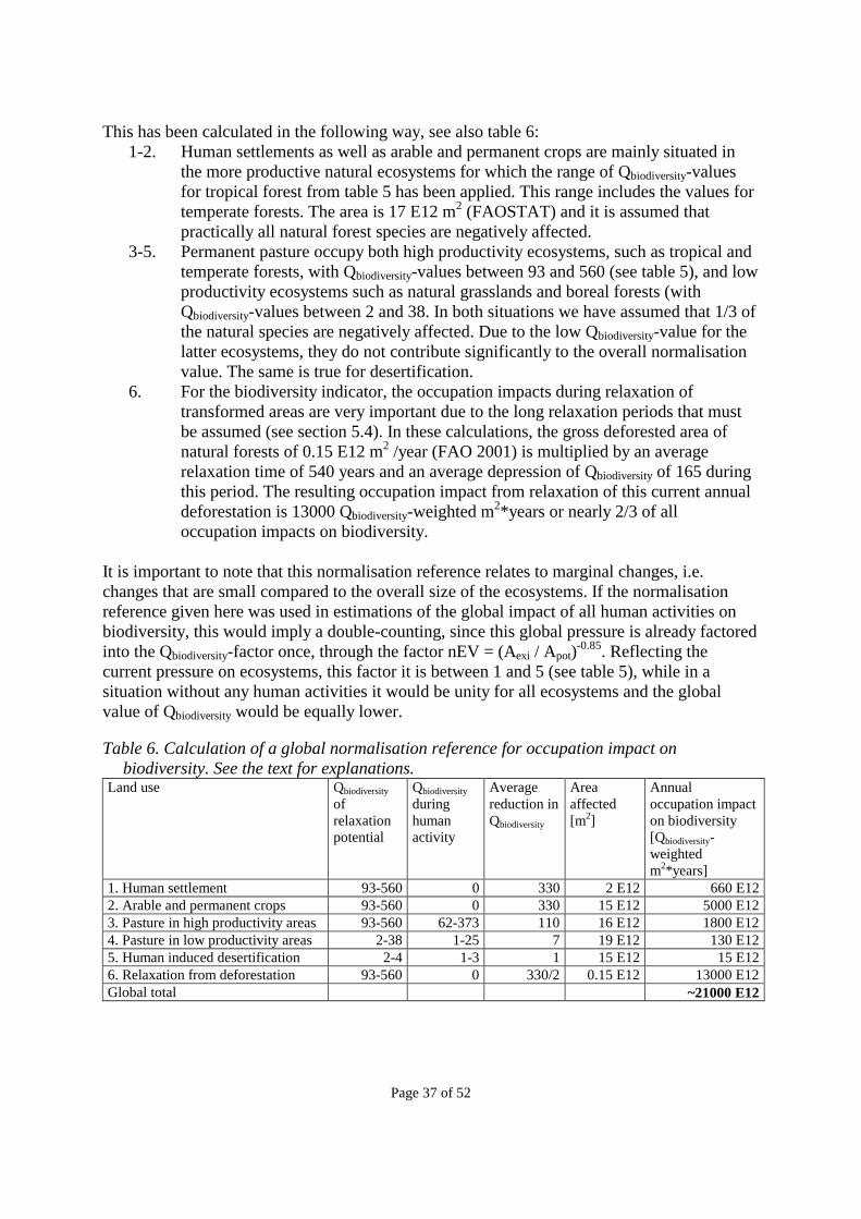
Page 37 of 52

This has been calculated in the following way, see also table 6:

1-2. Human settlements as well as arable and permanent crops are mainly situated in the more productive natural ecosystems for which the range of Qbiodiversity-values for tropical forest from table 5 has been applied. This range includes the values for temperate forests. The area is 17 E12 m2 (FAOSTAT) and it is assumed that practically all natural forest species are negatively affected.

3-5. Permanent pasture occupy both high productivity ecosystems, such as tropical and temperate forests, with Qbiodiversity-values between 93 and 560 (see table 5), and low productivity ecosystems such as natural grasslands and boreal forests (with Qbiodiversity-values between 2 and 38. In both situations we have assumed that 1/3 of the natural species are negatively affected. Due to the low Qbiodiversity-value for the latter ecosystems, they do not contribute significantly to the overall normalisation value. The same is true for desertification.

6. For the biodiversity indicator, the occupation impacts during relaxation of transformed areas are very important due to the long relaxation periods that must be assumed (see section 5.4). In these calculations, the gross deforested area of natural forests of 0.15 E12 m2 /year (FAO 2001) is multiplied by an average relaxation time of 540 years and an average depression of Qbiodiversity of 165 during this period. The resulting occupation impact from relaxation of this current annual deforestation is 13000 Qbiodiversity-weighted m2*years or nearly 2/3 of all occupation impacts on biodiversity.

It is important to note that this normalisation reference relates to marginal changes, i.e. changes that are small compared to the overall size of the ecosystems. If the normalisation reference given here was used in estimations of the global impact of all human activities on biodiversity, this would imply a double-counting, since this global pressure is already factored into the Qbiodiversity-factor once, through the factor nEV = (Aexi / Apot)

-0.85. Reflecting the current pressure on ecosystems, this factor it is between 1 and 5 (see table 5), while in a situation without any human activities it would be unity for all ecosystems and the global value of Qbiodiversity would be equally lower. Table 6. Calculation of a global normalisation reference for occupation impact on

biodiversity. See the text for explanations. Land use Qbiodiversity

of relaxation potential

Qbiodiversity during human activity

Average reduction in Qbiodiversity

Area affected [m2]

Annual occupation impact on biodiversity [Qbiodiversity-weighted m2*years]

1. Human settlement 93-560 0 330 2 E12 660 E12 2. Arable and permanent crops 93-560 0 330 15 E12 5000 E12 3. Pasture in high productivity areas 93-560 62-373 110 16 E12 1800 E12 4. Pasture in low productivity areas 2-38 1-25 7 19 E12 130 E12 5. Human induced desertification 2-4 1-3 1 15 E12 15 E12 6. Relaxation from deforestation 93-560 0 330/2 0.15 E12 13000 E12 Global total ~21000 E12

Page 38 of 52

4. Implications for inventory In the context of LCA, the concepts, indicators, and data described in the previous chapters would not be meaningful if they could not be related to the product life cycle inventory data, i.e. the available data on land use for specific human activities. Therefore, this chapter looks at the possibilities to record: �� The location of a specific human activity �� The size of the area affected �� The current relaxation potential for the affected area �� Relaxation periods

4.1 Typical locations of specific human activities

In LCA, the human activities that are involved in the production of a specific product can often be determined only in terms of their general nature, such as “tin extraction” or “soy bean production.” In some instances, the geographical location can be determined, at least at the level of country. For the indicators described in chapter 2 and 3, the location needs to be described in terms of ecosystem characteristics. A default solution to this problem would be simply to apply the average country-wise location of each activity type, e.g. all tin or soy bean producing countries would be assumed to be affected in proportion to their share of the global production, and within each country, all ecosystems would be assumed to be affected in proportion to their share in the total area. An example of this approach for resource extraction can be found in Lindeijer et al. (1998), see table 6.

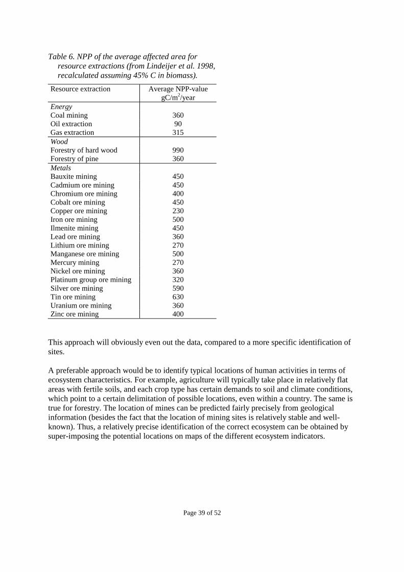
Page 39 of 52

Table 6. NPP of the average affected area for resource extractions (from Lindeijer et al. 1998, recalculated assuming 45% C in biomass).

Resource extraction Average NPP-value gC/m2/year

Energy Coal mining 360 Oil extraction 90 Gas extraction 315 Wood Forestry of hard wood 990 Forestry of pine 360 Metals Bauxite mining 450 Cadmium ore mining 450 Chromium ore mining 400 Cobalt ore mining 450 Copper ore mining 230 Iron ore mining 500 Ilmenite mining 450 Lead ore mining 360 Lithium ore mining 270 Manganese ore mining 500 Mercury mining 270 Nickel ore mining 360 Platinum group ore mining 320 Silver ore mining 590 Tin ore mining 630 Uranium ore mining 360 Zinc ore mining 400

This approach will obviously even out the data, compared to a more specific identification of sites. A preferable approach would be to identify typical locations of human activities in terms of ecosystem characteristics. For example, agriculture will typically take place in relatively flat areas with fertile soils, and each crop type has certain demands to soil and climate conditions, which point to a certain delimitation of possible locations, even within a country. The same is true for forestry. The location of mines can be predicted fairly precisely from geological information (besides the fact that the location of mining sites is relatively stable and well-known). Thus, a relatively precise identification of the correct ecosystem can be obtained by super-imposing the potential locations on maps of the different ecosystem indicators.

Page 40 of 52

4.2 Size of area affected

For agriculture and forestry, the area affected for a specific production can be readily calculated from data on yields per hectare (FAOSTAT http://apps.fao.org/). For mining and other activities, data are available in several LCA databases, e.g. the ETH data (Frischknecht et al. 1996) and the IVAM database (http://www.ivambv.uva.nl/uk/producten/product5.htm).

4.3 Current relaxation potentials

For biodiversity, the extinction of species at the global level will imply a reduction in the biodiversity relaxation potential, in proportion to the reduction in global species density for that ecosystem caused by the land use. As the vulnerability of the particular ecosystem has already been factored into the Qbiodiversity in section 2.3, it is reasonable to assume for all ecosystems a fixed percentage of Qbiodiversity being affected by a similar size of area occupied. To calculate this percentage, the method suggested by Müller-Wenk (1998) may be appropriate. For German conditions, Müller-Wenk calculates the marginal effect of land use on biodiversity to be 0.00005% per incremental km2*year occupied, or 5 * 10-13 per m2*year. To fit the formula of Qbiodiversity from section 2.3, the percentage should be established for the least valuable/threatened ecosystem, but in the absence of such data the percentage given for German conditions could be used as a “better-than-nothing” value. This would imply, for example, that an occupation of 70 km2 of an area with a Qbiodiversity of 160 (typical of rainforest) for a period of 180 years, would be attributed a permanent reduction in Qbiodiversity

of 0.0000005/km2/year * 70km2 * 160 * 180years = 1. For net primary production, the current relaxation potential can generally be assumed to be the climax ecosystem, as described by the indicators and data in chapter 2 and 3. The exception is instances where prior or current land use has altered the physical conditions to an extent that a full recovery to the climax ecosystem is prevented. This may be caused by nutrient depletion or enrichment, soil compaction, pollutants, or dominance by invasive species. We are not aware of any studies that have determined the relaxation potential in such human-influenced ecosystems, and must therefore recommend a case-by-case approach.

4.4 Current indicator level for different human activities

Land uses will differ in their degree of influence on the indicators described in chapter 2 and 3. The complete removal of all vegetation and sealing of the surface (e.g. for buildings and roads) is one extreme, to which open mining sites also belong. The other extreme is the hunting of one particular species, which may or may not affect overall ecosystem functions, depending on the constraints on the particular hunting and the role of that species within the ecosystem. In between these extremes we find different silvi- and agricultural land uses as

Page 41 of 52

well as residential areas and recreative and military use of land, which may in some instances increase the “nature quality” of an area, in other cases reduce it, but generally not to zero. For the indicators related to substance cycles and ecosystem productivity, the identification of the indicator level of the current land use is straightforward. Heavy grazing has small negative effect on NPP (Milchunas et al. 1994), which may be estimated to 15% of the NPP of the corresponding natural grasslands. For arable lands, especially in developing countries, the NPP may be as low as 10-20% of the NPP of the native vegetation, and only in the most developed countries can NPP of arable land exceed that of the native vegetation (Esser, 1994). The net primary productivity of crops may be estimated from crop yields by applying the crop-specific coefficients of dry matter content, harvest index, root production, and carbon and nitrogen content provided by Goudriaan (1997). For silviculture, management practices may influence net primary productivity, typically in an upward direction, but in general it can be assumed that there is no difference relative to the NPP of natural forests. For residential areas, a default value of 100 g C per m2 per year can be used, while for recreative and military use of land, the estimates may be based on a qualitative assessment of the degree of deviation from the current relaxation potential. For the biodiversity indicator, it is less straightforward to identify the indicator level for current land use. While the overall species richness may increase, be stable, or decrease under human land use, most land uses will favour some species at the expense of others. The use of species richness as such would therefore not correctly reflect the threat to biodiversity. Rather, the current indicator level should reflect the relative number of species not negatively affected by the current land use. Approximately 1/3 of naturally occurring rangeland species may be negatively affected by increased grazing (Landsberg et al. 1997). Most arable farming will imply a complete replacement of the naturally occurring ecosystem, and will therefore receive a zero score, equivalent to mining activities and residential use6. For silvicultural and recreative land uses, the relative number of species not negatively affected will depend heavily on management practices, and estimates need therefore to be based on an assessment of the specific management practice (see e.g. Hansen et al. 1991). For biodiversity indicators of managed forests, see also Bachmann et al. (1996) and Hansson (2000).

4.5 Relaxation periods

Tentative data for the relaxation period required to reach maximum potential biomass after a complete system removal, and under the assumption of no degradation in the relaxation potential, is given by Dobben et al. (1998), see table 7. The relaxation period to reach maximum potential biodiversity will be much longer. A tentative value can be obtained by multiplying the values in table 7 with a factor 6.

6 This does not imply a neglect of agricultural or horticultural diversity, but rather that the maintenance of this aspect of biodiversity needs to be captured by a separate indicator, additional to the indicator for biodiversity of natural systems described in this paper.

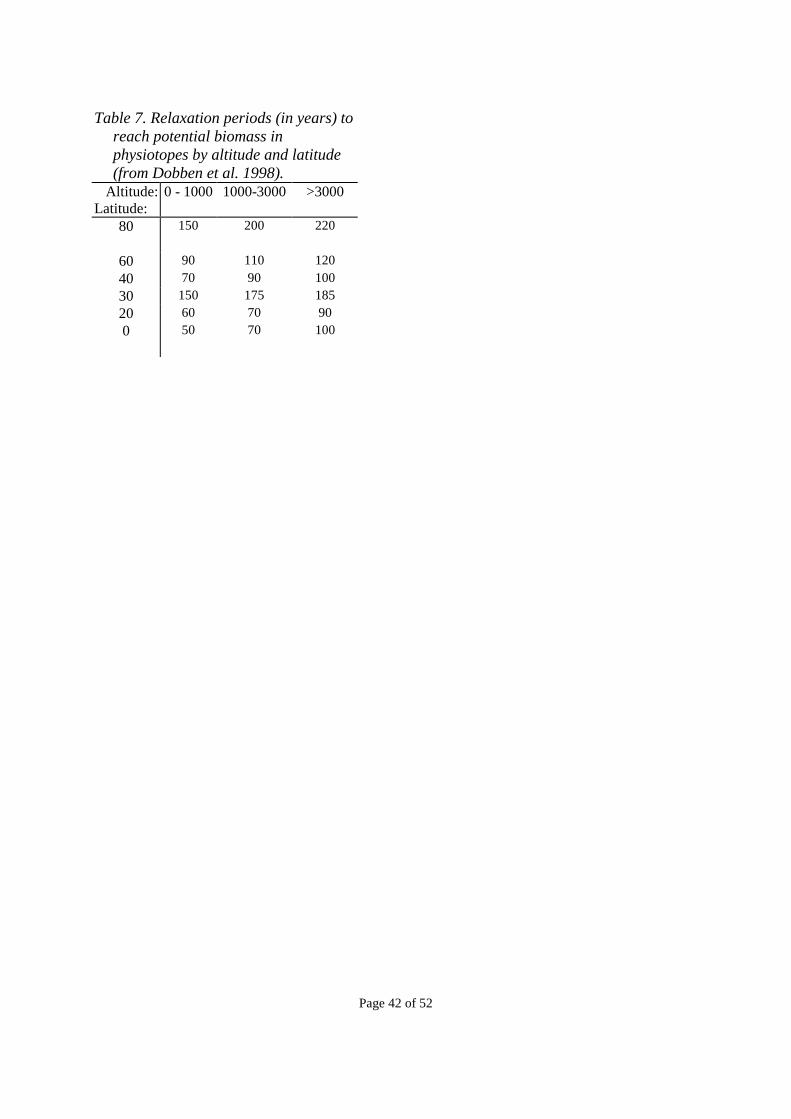
Page 42 of 52

Table 7. Relaxation periods (in years) to

reach potential biomass in physiotopes by altitude and latitude (from Dobben et al. 1998).

Altitude: Latitude:

0 - 1000 1000-3000 >3000

80 150 200 220

60 90 110 120

40 70 90 100

30 150 175 185

20 60 70 90

0 50 70 100

Page 43 of 52

5. Examples As examples of the application of the methodology outlined in chapters 1 to 4, we have chosen a few typical products: soybean, rapeseed, sand, beef and road transport. The examples deal exclusively with the indicators for ecosystem productivity and biodiversity. Furthermore, we have not included possible changes in the areas surrounding the investigated human activities. Soybean production for European market The current trend in soybean production is an increase in cultivated area, especially in Brazil, where new land is taken into cultivation. Thus, the marginal soybean production implies a land transformation from the natural biome (tropical forest) in Brazil (latitude around 20�) to agriculture. For 1000 kg soybeans, the occupation impact can be calculated as follows (see also table 8):

1. The area (A) transformed and occupied during the activity is 4250 m2 calculated from a yield of 2350 kg/ha/yr according to FAOSTAT.

2. The duration of the activity (tact) is 1 year, and the relaxation time (trelax) for latitude 20� is 60 years for ecosystem productivity and 360 years for biodiversity (see section 4.5).

3. Qpot, productivity in the relaxation potential (assuming no permanent ecosystem impact) is 720 g C/m2/year (from table 3). Qpot, biodiversity in the relaxation potential is 155, calculated from formula 7: (SR / SRmin) * (Apot,max / Apot) * (Aexi / Apot)

-0.85, with an intermediate value for SR = 2500 species/10000 km2; SRmin = 100 species/10000 km2 and data for tropical forest from table 5: Apot,max = 25.3 * 106; Apot = 5.7 * 106; Aexi = 3.8 * 106.

4. Qact, productivity during soybean production is 420 g C/m2/year (assuming a grain to NPP ratio of 0.25 and 45% C in biomass). Qact, biodiversity in soybean production is zero, as there are none of the original species left on the area.

5/6. During the production, the above quality is maintained constant, while during relaxation the quality increases gradually from the actual quality level of the production to the level of the relaxation potential. Thus, during production, the reduction in quality is simply the difference between the potential and the actual levels, while during relaxation this difference is gradually diminished. Assuming an even curve between the two levels (whether straight or sigmoid), the quality will on average be half of the difference between the potential level and the level during production. This is reflected in the slope factor s = 2 during relaxation.

7. The occupation impact can then be calculated from the formula:

Iocc = A * ti * (Qpot - Qact)/si (8) where the index i signifies either “activity” for the period during soybean growing or “relaxation” for the relaxation period, and finally the separately calculated values for these two periods can be added, resulting in the values 39.5 * 103 kg C for ecosystem productivity and 119 * 106 Qbiodiversity-weighted m2*years for biodiversity.

Page 44 of 52

These values can be normalised and expressed in person-equivalents by dividing by the normalisation references from section 3.2 and 3.3: 1750 kg C / capita / year and 3.8 * 106 Qbiodiversity-weighted m2*years/capita/year, respectively, resulting in the following normalised values per 1000 kg soy-beans: 22.6 person-equivalents for ecosystem productivity and 52.4 person-equivalents for biodiversity. The fairly large normalised values reflect that soybean production involves land transformation that constitutes an important part of the global impact. Table 8. Calculation of the occupation impact from growing 1000 kg soy beans Impact on

ecosystem productivity during activity

Impact on ecosystem productivity during relaxation

Impact on biodiversity during activity

Impact on biodiversity during relaxation

1. Area A 4250 m2 4250 m2 4250 m2 4250 m2 2. Time tact and trelax 1 year 60 years 1 year 360 years 3. Potential

quality Qpot 720

g C/m2/year 720

g C/m2/year 155 155

4. Actual quality Qact 420 g C/m2/year

420 g C/m2/year

0 0

5. Slope factor s 1 2 1 2 6. Quality

reduction Qred = (Qpot - Qact)/s

300 g C/m2/year

150 g C/m2/year

155 77.5

7. Occupation impact

Iocc = A * t i * Qred

39.5 * 103 kg C

119 * 106 Qbiodiversity-weighted m2*years

The permanent ecosystem impact on biodiversity can be calculated by multiplying the 119 * 106 Qbiodiversity-weighted m2*years with the factor 5 * 10-13/m2/year from section 4.3, resulting in a Qbiodiversity-value of 6 * 10-5. Rape seed production for European market Rape seed is currently a crop grown on set aside areas in Europe, where the trend is that agricultural land is taken out of cultivation. Rape seed production can therefore be seen as a simple postponement of relaxation in the natural biome temperate deciduous forest. For 1000 kg rapeseed, the impact can be calculated as follows (see also table 9):

1. The area (A) occupied during the activity is 4000 m2 calculated from a yield of 2500 kg/ha/yr according to FAOSTAT.

2. The duration of the activity (tact) is 1 year. As there is no transformation, there is no relaxation time allocated to this activity.

3. Qpot, productivity in the relaxation potential at latitude 40� is 540 g C/m2/year (from table 3). Qpot, biodiversity in the relaxation potential is 192, calculated from formula 7, with SR = 1000 species/10000 km2 and data for temperate deciduous forest from table 5: Apot = 6.2 * 106; Aexi = 1.0 * 106.

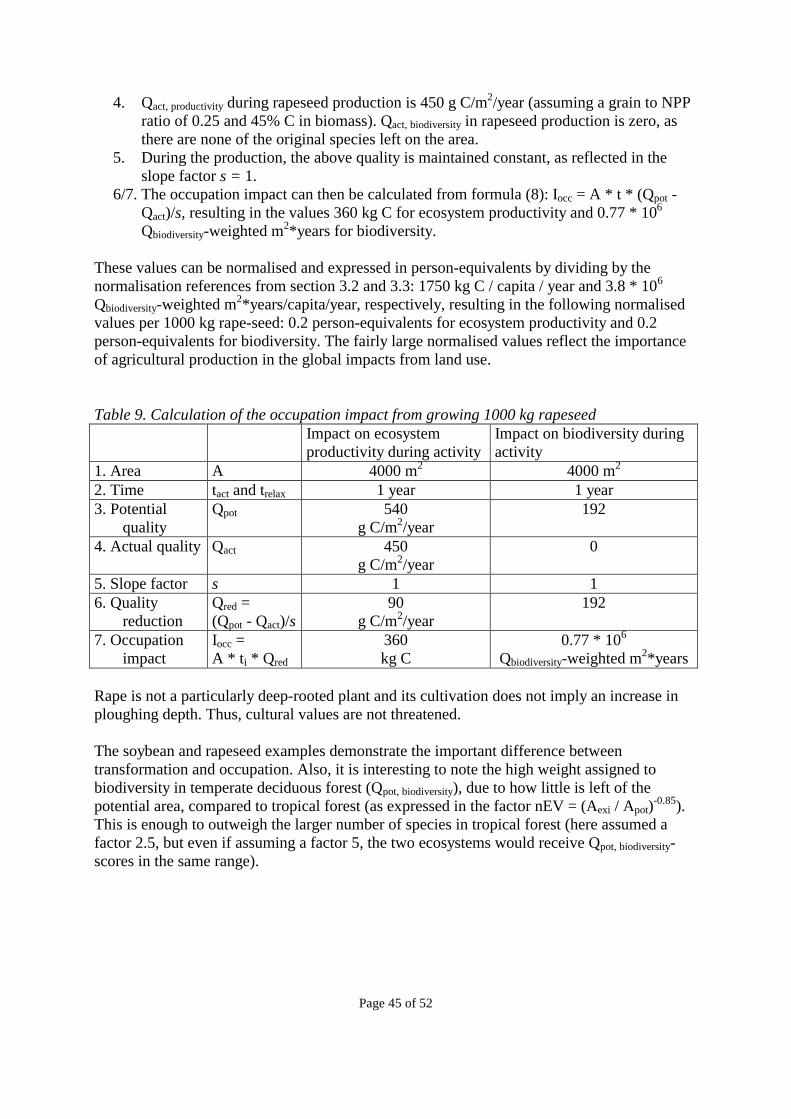
Page 45 of 52

4. Qact, productivity during rapeseed production is 450 g C/m2/year (assuming a grain to NPP ratio of 0.25 and 45% C in biomass). Qact, biodiversity in rapeseed production is zero, as there are none of the original species left on the area.

5. During the production, the above quality is maintained constant, as reflected in the slope factor s = 1.

6/7. The occupation impact can then be calculated from formula (8): Iocc = A * t * (Qpot - Qact)/s, resulting in the values 360 kg C for ecosystem productivity and 0.77 * 106 Qbiodiversity-weighted m2*years for biodiversity.

These values can be normalised and expressed in person-equivalents by dividing by the normalisation references from section 3.2 and 3.3: 1750 kg C / capita / year and 3.8 * 106 Qbiodiversity-weighted m2*years/capita/year, respectively, resulting in the following normalised values per 1000 kg rape-seed: 0.2 person-equivalents for ecosystem productivity and 0.2 person-equivalents for biodiversity. The fairly large normalised values reflect the importance of agricultural production in the global impacts from land use. Table 9. Calculation of the occupation impact from growing 1000 kg rapeseed Impact on ecosystem

productivity during activity Impact on biodiversity during activity

1. Area A 4000 m2 4000 m2 2. Time tact and trelax 1 year 1 year 3. Potential

quality Qpot 540

g C/m2/year 192

4. Actual quality Qact 450 g C/m2/year

0

5. Slope factor s 1 1 6. Quality

reduction Qred = (Qpot - Qact)/s

90 g C/m2/year

192

7. Occupation impact

Iocc = A * t i * Qred

360 kg C

0.77 * 106 Qbiodiversity-weighted m2*years

Rape is not a particularly deep-rooted plant and its cultivation does not imply an increase in ploughing depth. Thus, cultural values are not threatened. The soybean and rapeseed examples demonstrate the important difference between transformation and occupation. Also, it is interesting to note the high weight assigned to biodiversity in temperate deciduous forest (Qpot, biodiversity), due to how little is left of the potential area, compared to tropical forest (as expressed in the factor nEV = (Aexi / Apot)

-0.85). This is enough to outweigh the larger number of species in tropical forest (here assumed a factor 2.5, but even if assuming a factor 5, the two ecosystems would receive Qpot, biodiversity-scores in the same range).

Page 46 of 52

Sand extraction for European market Sand extraction in Europe is located in areas formerly used for agriculture. In some instances, the site is not restored after the termination of the extraction process but instead left as e.g. a lake, implying a permanent ecosystem change. In other instances, the ground is restored after the extraction and the extraction can therefore be seen as a simple postponement of relaxation in the natural biome temperate deciduous forest. In the latter case, the occupation impact per 1000 kg sand can be calculated as: �� Area*time occupied: 0.18 m2*years (from Lindeijer et al. 1998). �� Qpot, productivity in the relaxation potential: 540 g C/m2/year (as for rape, see this). �� Qpot, biodiversity in the relaxation potential: 192 (as for rape, see this). �� Qact, productivity during sand extraction: zero. �� Qact, biodiversity during sand extraction: zero �� Occupation impact: 540 gC/m2/year * 0.18 m2 = 0.097 kg C for ecosystem productivity

and 192 * 0.18 m2*years = 35 Qbiodiversity-weighted m2*years for biodiversity. These values can be normalised and expressed in person-equivalents by dividing by the normalisation references from section 3.2 and 3.3: 1750 kg C / capita / year and 3.8 * 106 Qbiodiversity-weighted m2*years/capita/year, respectively, resulting in the following normalised values per 1000 kg sand: 0.055 milli-person-equivalents for ecosystem productivity and 0.009 milli-person-equivalents for biodiversity. As sand extraction involves the complete removal of soil to a great depth, there may be a significant impact on cultural values (see section 2.4), unless particular precautions are taken. Beef production in Europe The marginal beef production is taking place on permanent grasslands, which are currently being taken out of cultivation. Thus, beef production can be seen as a simple postponement of relaxation in the natural biome. If the natural biome is assumed to be temperate deciduous forest, the calculation will be parallel to the above. However, an assessment at the biome level will not reflect that permanent grasslands may be placed in biotopes quite different from the average biome area, and thus stresses the importance of improving the availability of indicators at lower ecosystem levels than biome, as suggested in chapter 2. Road transport in Europe Road transport is mainly taking place between high-density population centres placed in fertile areas. Although areas for roads are therefore often taken out of agricultural use, and the trend is an increase in area for infrastructure, the general trend for agricultural land is a reduction of cultivated area, also beyond that which is transferred to other human use. Thus, roads can be seen as a simple postponement of relaxation in the natural biome temperate deciduous forest, and the calculation will be parallel to the above, with area*time being 0.004-0.021 m2*year per t*km transport (Lindeijer et al. 1998). It should be noted that roads often have considerable effects on the neighbouring areas.

Page 47 of 52

References Amthor J S, members of the Ecosystems Working Group. (1998). Terrestrial Ecosystem

Responses to Global Change: a research strategy. Oak Ridge: Oak Ridge National Laboratory. (ORNL Technical Memorandum 1998/27).

Arrhenius, O. (1921). Species and area. Journal of Ecology 9:95-99. Bachmann P, Michael K, Päivinen R. (eds.) (1996). Assessment of Biodiversity for Improved

Forest Planning. Proceedings of the conference “Assessment of Biodiversity for Improved Forest Planning” Monte Verità, Ascona, 1996.10.07-11. (Kluwer Forestry Sciences 51).

Baitz M, Kreissig J, Schöch C. (1998). Methode zur Integration der Naturraum-Inanpruchnahme in Ökobilanzen. Stuttgart: IKP, Universität Stuttgart.

Barbier E, Burgess J, Folke C. (1994). Paradise lost? The ecological economics of biodiversity. London: Earthscan.

Barthlott W, Lauer W, Placke A. (1996). Global distribution of species diversity in vascular plants: towards a world map of phytodiversity. Erdkunde 50(4):317-327.

Barthlott W, Biedinger N, Braun G, Feig F, Kier G, Mutke J. (1999). Terminological and methodological aspects of the mapping and analysis of global biodiversity. Acta Botanica Fennica 162: 103-110.

Blonk T J, Lindeijer E W. (1995). Naar een methoediek voor het kwantificeren van aantasting in LCA. Delft: Rijkswaterstaat, Dienst Weg- en Waterbouwkunde. (Publicatiereeks Grondstoffen 1995/15).

Blonk T J, Broers J W, Lindeijer E. (1996). Towards a methodology for characterisation of ecosystem degradation in LCA. Presentation for 6th SETAC-Europe Annual Meeting, Taormina, 1996.05.19-22.

Box E O. (1995). Global potential natural vegetation: dynamic benchmark in the era of disruption. Pp. 77-96 in Murai S.: Towards global planning of sustainable use of the earth. Amsterdam: Elsevier.

Connor E F, McCoy E D. (1979). The statistics and biology of the species-area relationship. American Naturalist 113: 791-833.

Cowell S. (1998). Environmental life cycle assessment of agricultural systems: Integration into decision-making. Ph.D. dissertation. Guildford: Centre for Environmental Strategy, University of Surrey.

Daily G. (ed.) (1997). Nature’s services: Societal dependence on natural ecosystems. Washington DC: Island.

Dalla Bona L. (1994). Methodological considerations. Thunder Bay: Lakehead University, Center for Archaeological Resource Prediction. (Volume 3 of a report series for the Ontario Ministry of Natural Resources).

Dankers N, Leopold M F. (1998). Biodiversity as a basis for evaluating impacts in marine benthic systems in LCA. Annex 2 in Lindeijer et al. (see this).

Dobben H F, Schouwenberg E P A G, Nabuurs G J, Prins A H. (1998). Biodiversity and productivity parameters as a basis for evaluating land use changes in LCA. Annex 1 in Lindeijer et al. (see this).

FAO. (2001). The global forest resources assessment 2000. Summary report. Information note for item 8(b) of the provisional agenda for the 15th session of the Committee on Foresty 2000.03.12-16. Rome: FAO. (ftp://ftp.fao.org/unfao/bodies/cofo/cofo15/X9835e.doc).

FAOSTAT. http://apps.fao.org/

Page 48 of 52

Farmer A J, Wiens J A. (in press). Optimal migration schedules depend on the landscape and the physical environment: a dynamic modeling view. Journal of Avian Biology.

Esser G. (1994). Eingriffe der Landwirtschaft in den Kohlenstoffkreislauf. In: Enquete-Kommission "Schutz der Erdatmosphäre" des Deutschen Bundestages (ed.): Landwirtschaft. Studienprogramm. Band 1. Bonn: Economica.

Frischknecht R, Bollens U, Bosshart S, Ciot M, Ciseri L, Doka G, Hischier R, Martin A, Dones R, Gantner U. (1996). Ökoinventare von Energiesystemen. Grundlagen für den ökologischen Vergleich von Energiesystemen und den Einbezug von Energiesystemen in Ökobilanzen für die Schweiz. 3rd Edition. Zürich: ETH, Gruppe Energie - Stoffe – Umwelt.

Gillette D. (1978). A wind tunnel simulation of the erosion of soil. Atmospheric Environment 12:1735-1743.

Goedkoop M, Spriensma R. (1999). The Eco-Indicator 99. Amersfoort: PRé Consultants. Goudriaan J. Groot J J R, Uithol P W J. (1997). Global Productivity of Agricultural Crops.

Proceedings of an International Workshop on Simulation of Agricultural and Environmental Systems, Lisbon, 1997.09.08-17. (Published in Revista de Ciências Agrárias 1999 vol. 22(1)).

Green M J B, Paine J. (1997). State of the World’s protected areas at the end of the twentieth century. Paper presented at IUCN World Commission on Protected Areas Symposium on “Protected Areas in the 21 st Century: From Islands to Networks” Albany, 1997.11.24-29. Cambridge: World Conservation Monitoring Centre (http://www.wcmc.org.uk/).

Groombridge B. (ed.) (1992). Global biodiversity. Status of the Earth’s Living Resources. London: Chapman & Hall.

de Groot R S. (1987). Environmental functions as a unifying concept for ecology and economics. Environmentalist 7:105-109.

de Groot R S. (1992). Functions of nature. Groningen: Wolters-Noordhoff. Hansen A J, Spies T A, Swanson F J, Ohmann J L. (1991). Conserving biodiversity in

managed forests. BioScience 41:382-392. Hansson L. (2000). Indicators of biodiversity: recent approaches and some general

suggestions. Stockholm: Swedish Environmental Protection Agency. (BEAR Technical report 1, updated version).

Heijungs R, Guinée J. (1997). Impact categories for natural resources and land use. Leiden: Centre for Milieukunde, Rijks Universiteit Leiden. (CML report 18)

Huang Y, Sass R L, Fisher F M. (1997). Methane emissions from Texas rice paddy soils. Global Change Biology.

IUCN, UNEP, WWF. 1991. Caring for the Earth. A strategy for sustainable living. London: Earthscan.

Kier G, Barthlott W (in press). Measuring and Mapping endemism and species richness: a new methodological approach and its application on the flora of Africa. Biodiversity and Conservation.

Köllner T. (2000a). Species-pool effect potentials (SPEP) as a yardstick to evaluate land-use impacts on biodiversity. Journal of Cleaner Production 8: 293-311.

Köllner T. (2000b). The use of land in the product life-cycle and its consequences for ecosystem quality. Ph. D. Thesis. Zürich: Swiss Federal Institute of Technology, Natural and Social Science Interface.

Landsberg J, James C D, Morton S R, Hobbs T J, Stol J, Drew A, Tongway H. (1997). The effects of artificial sources of water on rangeland biodiversity. Alice Springs: CSIRO Division of Wildlife and Ecology.

Page 49 of 52

Leemans R, Kreileman E, Zuidema G, Alcamo J, Berk M, Van den Born G J, Den Elzen M, Hootsmans R, Janssen M, Schaeffer M, Toet A M C, De Vries H J M. (1998). The IMAGE User Support System: Global Change Scenarios from IMAGE 2.1. CD-rom. Bilthoven: National Institute of Public Health and the Environment. (RIVM Publication 4815006).

Lindeijer E W, van Kampen M, Fraanje P J, van Dobben H F, Nabuurs G J, Schouwenberg E P A G, Prins A H, Dankers N, Leopold M F. (1998). Biodiversity and life support indicators for land use impacts in LCA. Delft: Rijkswaterstaat, Dienst Weg- en Waterbouwkunde. (Publication series raw materials 1998/07).

Matthews E. (1983). Global vegetation and land use: new high resolution data bases for climate studies. Journal of Climate and Applied Meteorology 22:474-487.

Matthews E. (1993). Global geographical databases for modelling trace gas fluxes. International Journal of Geographical Information Systems 7(2):125-142.

Milchunas D G, Forwood J R, Lauenroth W K. (1994). Productivity of long-term grazing treatments in response to seasonal precipitation. Journal of Range Management 47(2):2133-2139.

Myers N, Simon J L. (1994). Scarcity or Abundance: A Debate on the Environment. New York: W W Norton.

Müller-Wenk R. (1998). Land use – The main threat to species. How to include land use in LCA. St. Gallen: Institut für Wirtschaft und Ökologie, Universität St.Gallen. (IWÖ-Diskussionsbeitrag 64).

Olson J S, Watts J A, Allison L J. (1985). Major world ecosystem complexes ranked by carbon in live vegetation. Oak Ridge: Carbon Dioxide Information Center, Oak Ridge National Laboratory. (NDP-017 http://cdiac.esd.ornl.gov/ftp/ndp017/table.html).

Prentice I C, Cramer W, Harrison S P, Leemans R, Monserud R A, Solomon A M. (1992). A global biome model based on plant physiology and dominance, soil properties and climate. Journal of Biogeography 19:117-134.

Prentice I C. Personal communication 1997 to Bo Weidema Prince S D, Goward S J. (1995). Global primary production: a remote sensing approach.

Journal of Biogeography 22:316-336. Reid W V, Miller K R. (1993). Keeping options alive: the scientific basis for conserving

biodiversity. Washington DC: World Resources Institute. Rosenzweig M L. (1995). Species Diversity in Space and Time. Cambridge University Press. Schmidt M. (1997). Biodiversitet og land-use i LCA-sammenhæng. Lyngby: Department of

Manufacturing Engineering and Management, Technical University of Denmark. Sellers P J, Randall D A, Collatz G J, Berry J A, Field C B, Dazlich D A, Zhang C, Collelo G D,

Bounoua L. (1996). A revised land surface parameterization (SiB2) for atmospheric GCMs - Part I: model formulation. Journal of Climate 9:676-705

Tegen I, Fung I. (1994). Modeling of mineral dust in the atmosphere: Sources, transport and optical thickness. Journal of Geophysical Research 99:22897-22914.

Tischendorf L, Fahrig L. (2000a). On the usage and measurement of landscape connectivity. Oikos 90(1).

Tischendorf L, Fahrig L. (2000b). How should we measure landscape connectivity? Landscape Ecology 15(7):633-641.

Turner K. (1991). Environment, economics and ethics. Pp. 209-224 in Pearce D. (ed.): Blueprint 2. Greening the world economy. London: Earthscan.

Udo de Haes H A, Jolliet O, Finnveden G, Hauschild M, Krewitt W, Müller-Wenk R (1999). Best available practice regarding impact categories and category indicators in life cycle impact assessment. Background document for the second working group on Life Cycle Impact Assessment of SETAC-Europe.

Page 50 of 52

USGS. (2000). http://edcwww.cr.usgs.gov/eros-home.html Weidema B P. (2000). Can resource depletion be omitted from environmental impact assessments?

Presentation to the 3rd SETAC World Congress, Brighton 2000.05.21-25. Weidema B P, Mortensen B. (1996). The treatment of land use in life cycle impact

assessment. Presentation for 6th SETAC-Europe Annual Meeting, Taormina, 1996.05.19-22.

van Wetten et al., 1996: The Netherlands and global depletion of biodiversity (in Dutch), AIDEnvironment, for the Ministry of VROM, Environmental Strategies Publications, NL

Williams P H, Humphries C J, Gaston K J. (1994). Centres of seed-plant diversity: the family way. Proceedings of the Royal Society London B256:67-70.

Vitusek P, Ehrlich P R, Ehrlich A H, Matson P. (1986) Human appropriation of the products of photosynthesis. Bioscience 36:368-373.

Page 51 of 52

Annex 1 Existing Aexi and potential Apot ecosystem areas on a simple biome level

Biosphere Atmosphere Transfer Scheme (USGS 2000)

Biome 2.0 model (Leemans et al., 1998); data from 1970

Existing biome / land use

Area [km2] (Aexi) Related potential biome

Area [km2] (Apot)

Land cover area (Aexi)

1 Crops, Mixed Farming 10 Irrigated crops Agriculture total

14339934 3362275

17702209

1 Agriculture 4 Extensive grassland Agriculture total

- 31513480 12311561

43825041 2 Short Grass, 7 Tall Grass Grassland total

10619309 9417805

20037114

11 Grassland/Steppe, 14 Savanna Grassland total

17170062 11534288

28704351

9016363 5390550

14406913 3 Evergreen Needleleaf Trees 6088235 6 Boreal forest 25332520 20721432 4 Deciduous Needleleaf Trees 2990132 7 Cool conifer forest 4722752 2441293 5 Deciduous Broadleaf Trees 5856440 9 Temp. Deciduous forest 6198476 1013739 6 Evergreen Broadleaf Trees 12819330 16 Tropical forest 5738681 3776888 (7 Tall Grass) (9417805) - -

8 Desert 11 Semidesert Desert total

15979128 12344809

28323937

12 Hot Desert 14181394 11567131

9 Tundra 7542839 4 Tundra, 5 Wooded tundra Tundra total

9029500 3076248

12105748

9537464 3774699

13312163 (10 Irrigated Crops) (3362275) - -

(11 Semidesert) (12344809) - -

12 Ice Caps and Glaciers 16573114 3 Ice 6660460

6684545

(13 Bogs and marches) (1385551) -

14 Inland Water, 15 Ocean

371478604 - -

13 Bogs and Marshes 16 Evergreen Scrubs 17 Deciduous Scrubs Scrubland total

1385551 1090829 3788346

6264726

13 Scrubland

8120857 2239859

18 Mixed Forest 3673596 8 Temp. mixed forest, 10 Warm mixed forest Mixed forest total

7689525 4759974

12449499

1714379 895506

2609885 19 Interrupted Forest 17746431 15 Tropical woodland 7622253 4254199 20 Water and Land Mixtures - - - Total land area (excluding inland water & oceans)

145618000 131000000 131000000

Page 52 of 52

Annex 2 Land classification schemes with their number codes: five from USGS and one (bold) from RIVM USGS Land Use/Land Cover System Legend (Modified Level 2)

IGBP Land Cover Legend

Simple Biosphere Model Legend

Simple Biosphere 2 Model Legend

Biosphere Atmosphere Transfer Scheme Legend

Biome 1 model (Potential vegetation)

Biome 2 model (Potential vegetation)

1 Urban and Built-Up Land 1 Evergreen Needleleaf Forest 1 Evergreen Broadleaf Trees 1 Broadleaf Evergreen Trees 1 Crops, Mixed Farming 1 Ice/Polar Desert 1 -

2 Dryland Cropland and Pasture 2 Evergreen Broadleaf Forest 2 Broadleaf Deciduous Trees 2 Broadleaf Deciduous Trees 2 Short Grass 2 Semidesert 2 -

3 Irrigated Cropland and Pasture 3 Deciduous Needleleaf Forest 3 Deciduous and Evergreen Trees

3 Broadleaf and Needleleaf Trees

3 Evergreen Needleleaf Trees 3 Tundra 3 Ice

4 Mixed Dryland/Irrigated Cropland and Pasture

4 Deciduous Broadleaf Forest 4 Evergreen Needleleaf Trees 4 Needleleaf Evergreen Trees 4 Deciduous Needleleaf Tree 4 Taiga 4 Tundra

5 Cropland/Grassland Mosaic 5 Mixed Forest 5 Deciduous Needleleaf Trees 5 Needleleaf Deciduous Trees 5 Deciduous Broadleaf Trees 5 Cold Deciduous Forest 5 Wooded tundra

6 Cropland/Woodland Mosaic 6 Closed Shrublands 6 Ground Cover with Trees and Shrubs

6 Short Vegetation/C4 Grassland

6 Evergreen Broadleaf Trees 6 Cool Grass/Shrub 6 Boreal forest

7 Grassland 7 Open Shrublands 7 Groundcover Only 7 Shrubs with Bare Soil 7 Tall Grass 7 Cool Conifer Forest 7 Cool conifer forest

8 Shrubland 8 Woody Savannas 8 Broadleaf Shrubs with Perennial Ground Cover

8 Dwarf Trees and Shrubs 8 Desert 8 Cold Mixed Forest 8 Temp. mixed forest

9 Mixed Shrubland/Grassland 9 Savannas 9 Broadleaf Shrubs with Bare Soil

9 Agriculture or C3 Grassland 9 Tundra 9 Cool Mixed Forest 9 Temp. deciduous forest

10 Savanna 10 Grasslands 10 Groundcover with Dwarf Trees and Shrubs

10 Water, Wetlands, Ice/Snow 10 Irrigated Crops 10 Temperate Decidous Forest 10 Warm mixed forest

11 Deciduous Broadleaf Forest 11 Permanent Wetlands 11 Bare Soil 11 Semidesert 11 Evergreen/Warm mixed Forest 11 Grassland/Steppe

12 Deciduous Needleleaf Forest 12 Croplands 12 Agriculture or C3 Grassland 12 Ice Caps and Glaciers 12 Warm Grass/Shrub 12 Hot desert

13 Evergreen Broadleaf Forest 13 Urban and Built-Up (missing in HTML-file) 13 Bogs and Marshes 13 Hot Desert 13 Scrubland

14 Evergreen Needleleaf Forest 14 Cropland/Natural Vegetation Mosaic

(missing in HTML-file) 14 Inland Water 14 Xerophytic Woods/Shrub 14 Savanna

15 Mixed Forest 15 Snow and Ice (missing in HTML-file) 15 Ocean 15 Tropical Rain Forest 15 Tropical woodland

16 Water Bodies 16 Barren or Sparsely Vegetated (missing in HTML-file) 16 Evergreen Shrubs 16 Tropical Seasonal Forest 16 Tropical forest

17 Herbaceous Wetland 17 Water Bodies 17 Persistent Wetland 17 Deciduous Shrubs 17 Tropical Dry Forest/Savanna

18 Wooded Wetland 18 Dry Coastal Complexes 18 Mixed Forest

19 Barren or Sparsely Vegetated 19 Water 19 Interrupted Forest

20 Herbaceous Tundra 20 Ice Cap and Glacier 20 Water and Land Mixtures

21 Wooded Tundra

22 Mixed Tundra

23 Bare Ground Tundra

24 Snow or Ice