Embed Size (px)
Citation preview

Ministry of Education and Science of the Russian Federation Saint Petersburg National Research University of Information
Technologies, Mechanics, and Optics
NANOSYSTEMS: PHYSICS, CHEMISTRY, MATHEMATICS
2016, volume 7 (5)
Наносистемы: физика, химия, математика 2016, том 7, 5
NANOSYSTEMS: PHYSICS, CHEMISTRY, MATHEMATICS
ADVISORY BOARD MEMBERS Chairman: V.N. Vasiliev (St. Petersburg, Russia), V.M. Buznik (Moscow, Russia); V.M. Ievlev (Voronezh, Russia), P.S. Kop’ev(St. Petersburg, Russia), N.F. Morozov (St. Petersburg, Russia), V.N. Parmon (Novosibirsk, Russia), A.I. Rusanov (St. Petersburg, Russia),
EDITORIAL BOARD Editor-in-Chief: I.Yu. Popov (St. Petersburg, Russia)
Section Co-Editors: Physics – V.M. Uzdin (St. Petersburg, Russia), Chemistry, material science –V.V. Gusarov (St. Petersburg, Russia), Mathematics – I.Yu. Popov (St. Petersburg, Russia).
Editorial Board Members: V.M. Adamyan (Odessa, Ukraine); O.V. Al’myasheva (St. Petersburg, Russia); A.P. Alodjants (Vladimir, Russia); S. Bechta (Stockholm, Sweden); J. Behrndt (Graz, Austria); M.B. Belonenko (Volgograd, Russia); V.G. Bespalov (St. Petersburg, Russia); J. Brasche (Clausthal, Germany); A. Chatterjee (Hyderabad, India); S.A. Chivilikhin (St. Petersburg, Russia); A.V. Chizhov (Dubna, Russia); A.N. Enyashin (Ekaterinburg, Russia), P.P. Fedorov (Moscow, Russia); E.A. Gudilin (Moscow, Russia); V.K. Ivanov (Moscow, Russia), H. Jónsson (Reykjavik, Iceland); A.A. Kiselev (Madison, USA); Yu.S. Kivshar (Canberra, Australia); S.A. Kozlov (St. Petersburg, Russia); P.A. Kurasov (Stockholm, Sweden); A.V. Lukashin (Moscow, Russia); V.A. Margulis (Saransk, Russia); I.V. Melikhov (Moscow, Russia); G.P. Miroshnichenko (St. Petersburg, Russia); I.Ya. Mittova (Voronezh, Russia); H. Neidhardt (Berlin, Germany); K. Pankrashkin (Orsay, France); A.V. Ragulya (Kiev, Ukraine); V. Rajendran (Tamil Nadu, India); A.A. Rempel (Ekaterinburg, Russia); V.Ya. Rudyak (Novosibirsk, Russia); D Shoikhet (Karmiel, Israel); P Stovicek (Prague, Czech Republic); V.M. Talanov (Novocherkassk, Russia); A.Ya. Vul’ (St. Petersburg, Russia); A.V. Yakimansky (St. Petersburg, Russia), V.A. Zagrebnov (Marseille, France).
Editors: I.V. Blinova; A.I. Popov; A.I. Trifanov; E.S. Trifanova (St. Petersburg, Russia), R. Simoneaux (Philadelphia, Pennsylvania, USA).
Address: University ITMO, Kronverkskiy pr., 49, St. Petersburg 197101, Russia. Phone: +7(812)232-67-65, Journal site: http://nanojournal.ifmo.ru/, E-mail: [email protected]
AIM AND SCOPE The scope of the journal includes all areas of nano-sciences. Papers devoted to basic problems of physics, chemistry, material science and mathematics inspired by nanosystems investigations are welcomed. Both theoretical and experimental works concerning the properties and behavior of nanosystems, problems of its creation and application, mathematical methods of nanosystem studies are considered. The journal publishes scientific reviews (up to 30 journal pages), research papers (up to 15 pages) and letters (up to 5 pages). All manuscripts are peer-reviewed. Authors are informed about the referee opinion and the Editorial decision.
N A N O
Ф &Х &М
CONTENT
I.Y.Popov, P.A. Kurasov, S.N. Naboko, A.A. Kiselev, A.E. Ryzhkov, A.M. Yafyasov, G.P. Miroshnichenko, Yu.E. Karpeshina, V.I. Kruglov, T.F. Pankratova, A.I. Popov A distinguished mathematical physicist Boris S. Pavlov 782 P. Exner, V. Lotoreichik, M. Tater On resonances and bound states of Smilansky Hamiltonian 789 S. Albeverio, S. Fassari, F. Rinaldi Spectral properties of a symmetric three-dimensional quantum dot with a pair of identical attractive δ-impurities symmetrically situated around the origin II 803 B. Pavlov, A. Yafyasov Resonance scattering across the superlattice barrier and the dimensional quantization 816 F. Al-Musallam, S. Avdonin, N. Avdonina, Ju. Edward Control and inverse problems for networks of vibrating strings with attached masses 835 A.S. Mikhaylov, V.S. Mikhaylov Dynamical inverse problem for the discrete Schrödinger operator 842 N.G. Kuznetsov On direct and inverse spectral problems for sloshing of a two-layer fluid in an open container 854 E.N. Grishanov, I.Y. Popov Computer simulation of periodic nanostructures 865 V.I. Korzyuk , N.V. Vinh Cauchy problem for some fourth-order nonstrictly hyperbolic equations 869 M. Muminov Spectral properties of a two-particle hamiltonian on a d-dimensional
lattice 880 F.H. Haydarov Characterization of the normal subgroups of finite index for the group representation of a Cayley tree 888 Yu.Kh. Eshkabilov, Sh.P. Bobonazarov, R.I. Teshaboev Translation-invariant Gibbs measures for a model with logarithmic potential on a Cayley tree 893 Information for authors 900
NANOSYSTEMS: PHYSICS, CHEMISTRY, MATHEMATICS, 2016, 7 (5), P. 782–788
A distinguished mathematical physicist Boris S. Pavlov
I. Y. Popov1, P. A. Kurasov2, S. N. Naboko3, A. A. Kiselev4, A. E. Ryzhkov1, A. M. Yafyasov3,G. P. Miroshnichenko1, Yu. E. Karpeshina5, V. I. Kruglov6, T. F. Pankratova1, A. I. Popov1
1ITMO University, Kronverkskiy, 49, St. Petersburg, 197101, Russia2Stockholm University, Stockholm, Sweden
3St. Petersburg State University, St. Petersburg, Russia4Rice University, Houston, Texas, USA
5University Alabama at Birmingham, USA6Centre for Engineering Quantum Systems, School of Mathematics and Physics,
The University of Queensland, Brisbane, QLD 4072, Australia∗[email protected]
PACS 01.60.+q DOI 10.17586/2220-8054-2016-7-5-782-788
Keywords: mathematical physics.
Received: 10 September 2016
Revised: 1 October 2016
Professor Boris Pavlov passed away on 30 January 2016.Boris Pavlov was born in Kronshtadt, Russia, 27 July 1936. He graduated from Physical faculty of Leningrad
State University in 1958 and continued to work at the Department of Mathematical Physics. His PhD thesis (1964,Supervisor – M. S. Birman) was devoted to investigation the spectrum of non-self-adjoint operator −y′′ + qy. Tenyears later, his PhD Thesis was followed by a Doctoral dissertation in Mathematical Analysis: “Dilation Theoryand Spectral Analysis of Nonselfadjoint Differential Operators”. He was a Vice-rector (Research) of LeningradUniversity [1978–1981 and at the same time [1978–1982], he had a Chair of Mathematical Analysis at the Facultyof Mathematics and Mechanics of Leningrad State University. Later [1982–1995] he worked as a Professor at thedepartment of Higher Mathematics and Mathematical Physics, Physics Faculty. The year 1995 was a branchingpoint for him. He held a Personal Chair in Pure Mathematics at the University of Auckland from 1994 to 2007,however, he did not break his connections with Russia. From 1995 he was a Chief of Complex Systems TheoryLaboratory at Physical Faculty. Since 2009, he was a member of the then newly formed Institute for AdvancedStudy at Massey University Albany.
B. S. Pavlov was well known for his high level of scholarship in diverse areas of analysis. He became aFellow of the Royal Society of New Zealand in 2004 and a member of the Russian Academy of Natural Sciencesin 2010. B. S. Pavlov leaves behind his wife Irina, a daughter and a son.
The highest scientific achievements of B. S. Pavlov (as he himself felt) are:
• Spectral theory of singular differential non-selfadjoint operators, 1962.• Riesz-basis property of exponentials on a finite interval, 1979.• Operator-theory interpretation of critical zeros of the Riemann zeta-function, 1972.• Symmetric Functional Model for dissipative operators, 1979.• Zero-range potentials with inner structure and solvable models, 1984.• Theory of the shift operator on a Riemann surface, jointly with S. Fedorov. 1987.• Modified analytic perturbation procedure (“Kick-start”) for operators with eigenvalues embedded into
continuous spectrum, 2005.• Fitting of zero-range solvable model of a quantum network based on rational approximation of the Dirichle-
to-Neumann map of the original Hamiltonian, 2007.• Fitted solvable model of the stressed tectonic plate, in connection with prediction of powerful earthquakes,
jointly with L. Petrova, 2008.• Quasi-relativistic dispersion and high mobility of electrons in Si-B sandwich structures, jointly with
N. Bagraev, 2009.• Theoretical interpretation of the low-threshold field emission from carbon nano-clusters, jointly with
Y. Fursey and A. Yafyasov, 2010.
A distinguished mathematical physicist Boris S. Pavlov 783
He supervised more than 30 students. Among them were:
1. V. L. Oleinik, Master,PhD student 1965–1971 (Associate Professor, St. Petersburg University)2. S. V. Petras, Master,PhD student 1965–1970 (Associate Professor, St. Petersburg University of Economics)3. M. G. Suturin, Master,PhD student 1966–1971 (Associate Professor, St. Petersburg Institute for Airspace
devices)4. S. N. Naboko, Master, PhD student 1969–1976 (Full Professor, St. Petersburg University)5. S. A. Avdonin, Master,PhD student 1969–1980 (Full Professor, the Univ. of Fairbancs, Alaska)6. M. A.Shubova, Master,PhD student 1969–1982 (Full Professor, the University of New Hampshire, USA)7. S. A. Ivanov, Master, PhD student 1972–1978 (Research worker at the Institute of Terrestrial Magnetism
RAS, St. Petersburg)8. I. Yu. Popov, Master, PhD student 1974–1978 (full Professor, Chair of Higher Mathematics, ITMO Univer-
sity, St. Petersburg)9. Yu. A. Kuperin, Master student 1975–1978 (Doctor of Science, Full Professor, St. Petersburg University)10. Y. E. Karpeshina, Master,PhD student 1975–1985 (Full Professor, Birmingham University, Alabama, USA)11. K. A. Makarov, Master, PhD student 1976–1982 (Full professor, Univ. Missouri-Columbia)12. S. E. Cheremshantsev, Master, PhD student 1976–1982 (Full Professor, Chair of Higher Mathematics,
Orlean University, France)13. A. V. Rybkin, Master, PhD student 1977–1982 (Full Professor, Univ. of Fairbancs, Alaska)14. A. V. Strepetov, Master, PhD student 1978–1986 (St. Petersburg Institute of Airspace devices, St. Peters-
burg, Russia)15. M. D. Faddeev, PhD student 1982–1985. (Associate Professor in St. Petersburg University)16. P. B. Kurasov, Master, PhD student 1981–1987 (Associate Professor, Doctor of science, now in Lund
University, Sweden)17. A. E. Ryzhkov, Master, PhD student 1974–1980 (Associate Professor, ITMO University, St. Petersburg)18. V. A. Evstratov, Master, PhD student 1984–1992 (Assistant Professor St. Petersbufg University till 1994.
Now in business)19. A. A. Shushkov, PhD student 1984–1987 (Assistant Professor St. Petersbufg University till 1991, now
somewhere in Canada)20. N. I. Gerasimenko, PhD student 1985–1987 (Associate Professor at the Higher Military School, St.
Petersburg)
784 I. Y. Popov, P. A. Kurasov, S. N. Naboko, et al.
21. M. M. Pankratov, Master, PhD student 1987–1991 (Insurance Company, Switzerland.)22. S. V. Frolov, Master, PhD student 1988–1993 (Doctor of Technology, Full Professor, ITMO University,
St.Petersburg)23. A. A. Pokrovski, Master, PhD student 1990–1995 (Research worker at the Institute for Physics of St.
Petersburg University, St. Petersburg, Russia)24. R. Killip, Master, PhD student, the Univ of Auckland 1994–1996 (Associate Professor, UCLA, Los-
Angeles, USA)25. J. Mac-Cormick, Master student, the Univ. of Auckland 1994–1995 (Research worker in Computer Design
Laboratory UCLA)26. A. Kraegeloh, Master thesis, the Univ. of Auckland 1995–1997 (Insurance company, Germany)27. M. Harmer, Master,PhD student Auckland 1996–2000 (Post Doc., Prague)28. A. B. Mikhailova, Master student 2000–2001, St-Petersburg Univ. (Research worker at the Institute for
Physics of St. Petersburg University)29. S. Mau, Master student, 1999–2002, the Univ of Auckland (PhD student, New York Univ., USA)30. S. Marshall, Master student, the Univ of Auckland 2004–2006 (PhD student at Princeton)31. S. Dillon, Master thesis, the Univ of Auckland, 2005–2007 (PhD at Massey Uni. NZ)
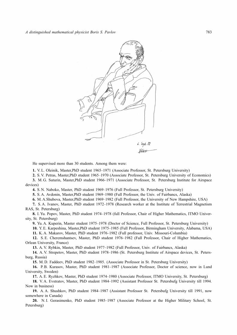
The scientific interests of B. S. Pavlov were very wide, ranging from quantum physics to earthquakes. Butwere not his only interests. He liked kayak travels and alpine skiing. Everybody knew him as a good painter. Inthis article, you can see his self-portrait. For his students, if they had a problem, they could visit Boris Sergeevich,as his door was always open and he would help them using all his abilities and talents. He was kind and wonderfulperson, a teacher in science and in life. We will never forget him.
To show particular remarkable features of B.S.Pavlov, we include here a few memories from his formerstudents.
A. Kiselev. I had the good fortune to study with Boris Sergeevich Pavlov for several years after I transferredfrom LITMO to SPbGU in 1989. Boris Sergeevich had set my early direction in mathematics, suggesting problemsto work on and topics to study. However, he did much more than that; he truly cared about his students, andprovided support and advice not only professionally but in other aspects of life. More than anything, though, heinfluenced me through his personal example of doing mathematics. For him, mathematics was something to liveand breathe, something to enjoy with friends and students. Boris Sergeevich treated his classes as performances,including a bit of occasional improvisation, making those instances some of the most inspiring moments I saw.He liked to say that mathematics is an experimental science. This way of thinking about mathematics – that oneshould build models, experiments, tirelessly explore the entire landscape surrounding the problem of interest – hasbecome part of my mathematical DNA.
Boris Sergeevich was very generous and gentle with me, but he did not hesitate to provide precise feedbackwhen something needed fixing. I remember my first ever presentation of research paper which I read in order tostart working on my own problem. Within five minutes of the start Boris Sergeevich yawned and stopped me andexplained that he does not need me to faithfully reproduce all the details. I am not at an exam now – what is theidea? This way my boring report quickly turned into a lively discussion. I am afraid that I could not tell the mainidea, however Boris Sergeevich did not let us fail and helped me formulate it in the end (I am pretty sure now hefigured it out long before I did but made me discover it myself). Every one of such interactions has been pricelessfor me. The friendly, supportive and wise guidance of Boris Sergeevich came at a key time in my education andtruly helped me grow as a mathematician.
P. Kurasov. I would like to mention B. S. Pavlov’s precepts for young scientists:Do other things than other researchers;Use other ways than other researchers;Look sharp during your research;Read, but do not read much, otherwise you will not be read;Do not disregard negative results;Do not “cram your results into explanation” before you have checked it carefully.
This article bibliography contains the papers of B. S. Pavlov in Refereed Journals.
References
[1] Pavlov B.S., Birman M.S. On the complete continuity of certain imbedding operators. Vestnik Leningrad. Univ. Math. Mekh. Astronom.,1961, 16(1), P. 61–74.
[2] Pavlov B.S. On non-selfadjoint operator on half-axis. USSR Acad. Sciences Doklady, 1961, 141(4), P. 807–810.[3] Pavlov B.S. On the spectral theory of non-self-adjoint differential operators. USSR Acad. Sciences Doklady, 1962, 146(6), P. 1267–1270.
A distinguished mathematical physicist Boris S. Pavlov 785
[4] Pavlov B.S., Nikolsky N.K. Eigenvector expansions of non-unitary operators, and the characteristic functions. Proceedings LOMI, 1968,2, P. 150–203.
[5] Pavlov B.S., Nikolsky N.K. Bases from eigenvectors, characteristic function and interpolation problems in Hardy classes. USSR Acad.Sciences Doklady, 1969, 184(3), P. 550–553.
[6] Pavlov B.S., Nikolsky N.K. Bases of eigenvectors of totally non-unitary contractions. USSR Acad. Sciences Doklady, 1969, 184(4),P. 778–781.
[7] Pavlov B.S., Nikolsky N.K. Bases of eigenvectors of completely non-unitary contractions and characteristic function. Izvestia USSR Acad.Sc., 1970, 34, P. 90–133.
[8] Pavlov B.S., Petras S.V. On singular spectrum of a weakly perturbed multiplication operator. Funct. Analysis and it’s applications, 1970,4(2), P. 54–61.
[9] Pavlov B.S. Scattering theory and nonphysical sheet for systems of ordinary differential equations. USSR Acad. Sc. Doklady, 1970, 193(1),P. 36–39.
[10] Pavlov B.S. The completeness of the set of resonance states for a system of differential equations. USSR Acad. Sc. Doklady, 1971, 196(6),P. 1272–1275.
[11] Pavlov B.S., Oleinik V.L. Embedding theorems for weight classes of harmonic and analytic functions. Proceedings LOMI, 1971, 22,P. 94–102.
[12] Pavlov B.S., Suturin M.G. The sharpness of certain embedding theorem. Proceedings LOMI, 1972, 30, P. 170–171.[13] Pavlov B.S. Factorization of scattering matrix and serial structure of it’s rootes. Izvestia USSR Acad. Sc., Math., 1973, 37, P. 217–246.[14] Pavlov B.S., Faddeev L.D. Scattering theory and automorphic functions. Proc.LOMI, 1972, 6(27), P. 161–193 (in Russian); (English
Transl.: J. Soviet Math. 1975, 3(4), Consultants bureau, New York-London).[15] Pavlov B.S. On one-dimensional scattering of plane waves on an arbitrary potential. Teor. i Mat. Fiz., 1973, 16(1), P. 105–119.[16] Pavlov B.S. The continuous spectrum of resonances on the nonphysical sheet. Soviet Math. Dokl., 1972, 13(5), P. 1301–1304.[17] Pavlov B.S. To the spectral analysis of dissipative operators. USSR Acad. Sc. Doklady, 1973, 212(2), P. 298–301.[18] Pavlov B.S. On expansion by eigenfunctions of absolutely continuous spectrum of a dissipative operator. Vestnik Leningrad University,
Math., 1975 1, P. 130–137.[19] Pavlov B.S. Conditions of separation for the spectral components of a dissipative operator Math. USSR Izvestija, 1975, 9(1), P. 113–137.[20] Pavlov B.S. Self-adjoint dilation of dissipative Schrodinger operator and expansion by it’s eigenfunctions. Func. Anal. i ego Prilogenia,
1975, 9(2), P. 87–88.[21] Pavlov B.S. Calculation of loses in scattering problems. Mat. Sbornik, 1975, 97(139), P. 77–93[22] Pavlov B.S., Smirnov N.V. Resonance scattering by one-dimensional crystall and thin film. Vestnik Leningrad University, (Phys.-Chem.),
1977, 13(3), P. XX.[23] Pavlov B.S., Faddeev M.D. Construction of self-adjoint dilation for the problem with the impedance boundary condition. Proc. LOMI,
1977, 73, P. 217–223.[24] Pavlov B.S., Ivanov S.A. Carleson resonance series in Regge problem. Izvestia USSR Acad. Sc., Math., 1978, 1, P. 26–55.[25] Pavlov B.S., Faddeev L.D. Zero sets of operator functions with the positive imaginary part. Proc. LOMI, 1978, 81, P. 85–88.[26] Pavlov B.S., Vasynin V.I., Nikolski N.K. Spectral expansions and Carleson condition. Proc. LOMI, 1978, 81.[27] Pavlov B.S., Beloserskij G.N. Method of estimations of the relaxation frequences of magnetisation vector for superparamagnetic particles.
Vestnik Leningrad University, 1978, 22, P. 12–19.[28] Pavlov B.S., Adamjan V.M. Trace formula for dissipative operator. Vestnik Leningrad University, math., 1979, 2. P. 5–9.[29] Pavlov B.S. Partial Scattering matrix, it’s factorization and analyticity. USSR Acad. Sc. Doklady, 1979, 244(2), P. 291–295.[30] Pavlov B.S. Basic property of a system of exponentials and the condition of Muckenhoupt. Soviet Math. Dokl., 1979, 21(1), P. 37–40.[31] Pavlov B.S., Beloserskij G.N. Motion of the magnetisation vector of superparamagnetic particles in stationary case. Journal of Magnetism
and magnetic materials, 1979, 12, P. 34–42.[32] Pavlov B.S., Ivanov S.A. Vector systems and zeros of entire matrix functions. Vestnik Leningrad University, Math., 1980, 2, P. 25–31.[33] Pavlov B.S., Beloserskij G.N., Semenov V.G., Korenev N.K. The time development of the magnetic moment of superparamagnetic particles
and discrete orientation model, II. Journal of Magnetism and magnetic materials, 1980, 20, P. 1–10.[34] Pavlov B.S., Beloserskij G.N., Makarov K.A. Discrete orientation model in the theory of superparamagnetism. Vestnik Leningrad Univer-
sity, Phys.-Chem., 1982, 4, P. 12–18.[35] Pavlov B.S., Faddeev M.D. Spectral analysis of unitary perturbations of contractions. Proc. LOMI, 1982, 115, P. 215–227 (In Rus-
sian)(English translation: J. of Sov.Math., 1985, 28, P. 768–776).[36] Pavlov B.S., Faddeev M.D. Scattering on a hollow resonator with the small opening. Proc. LOMI, 1983, 126, P. 159–169 (J. of Sov.Math.,
1984, 27, P. 2527–2533).[37] Pavlov B.S., Faddeev M.D. A model of free electrons and the scattering problem. Teor. i Mat. Fiz., 1983, 55(2), P. 257–268 (English
Translation: Theoret. and Math. Phys., 1983, 55(2), P. 485–492).[38] Pavlov B.S., Popov I.Yu. A model diffraction by infinitely narrow crack and the theory of extensions. (Russian). Vestnik Leningrad. Univ.
Mat. Mekh. Astronom. 1983, 19, P. 36–44.[39] Pavlov B.S., Smirnov N.V. Spectral properties of one-dimensional disperse crystals. (Russian). Proc. LOMI, 1984, 133, P. 197–211.[40] Pavlov B.S., Popov I.Yu. Scattering by resonators with the small and point holes. (Russian). Vestnik Leningrad. Univ. Math., 1984, 13,
P. 116–118.[41] Pavlov B.S. A model of zero-radius potential with internal structure. Teor.Mat.Fiz., 1984, 59(3), P. 345–354. (English translation: Theoret.
and Math. Phys, 1984, 59(3), P. 544–550).[42] Pavlov B.S., Popov I.Yu. A travelling wave in a ring resonator (Russian). Vestnik Leningrad. Univ. Phys.- Chem., 1985, 1, P. 99–102.[43] Pavlov B.S., Kuperin Yu.A., Makarov K.A. One-dimensional model of three-particle resonances. Teor. i Mat. Fiz., 1985, 63(1), P. 78–87
(English translation: Theoret. and Math. Phys., 1985, 63(1), P. 376–382).[44] Pavlov B.S., Karpeshina Yu.E. Interactions of the zero radius for the bi-harmonic and the poly-harmonic equations. Mat. Zametki, 1986,
40(1), P. 49–59. (English translation: Math. Notes, 1987, 40(1-2), P. 528–533).
786 I. Y. Popov, P. A. Kurasov, S. N. Naboko, et al.
[45] Pavlov B.S., Strepetov A.V. Simultaneous completeness in the case of a continuous spectrum. Funktsional. Anal. i Prilozhen., 1986, 20(1),P. 33–36. (English Translation: Functional Anal. Appl., 1986, 20(1), P. 27–30).
[46] Pavlov B.S., Adamjan V.M. Zero-radius potentials and M. G. Krein’s formula for generalized resolvents. Proc.LOMI, 1986, 149, P. 7–23.[47] Pavlov B.S., Popov I.Yu. Surface waves and extension theory. Vestnik Leningrad. Univ. Math., 1986, 4, P. 105–107 (In Russian).[48] Pavlov B.S., Kuperin Yu.A., Makarov K.A. Model of resonance scattering of compound particles. Teoret. Mat.Fiz., 1986, 69(1), P. 100–114
(Russian). (English Translation: Theoret. and Math. Phys. 69,1 (1986) P. 1028–1038).[49] Pavlov B.S. An electron in the homogeneous crystal of point-like atoms with internal structure I. Teor. i Mat. Fiz., 1987, 72(3), P. 403–415.[50] Pavlov B.S., Kuperin Yu.A., Makarov K.A. Scattering on a dynamical quark bag. Vestnik Leningrad Univ. Phys.- Chem., 1987, 4, P. 60–62.
(Russian)[51] Pavlov B.S. The spectral aspect of superconductivity – the pairing of electrons. Vestnik Leningrad. Univ. Math., 1987, 3, P. 43–49 (In
Russian).[52] Pavlov B.S. An explicitly solvable one-dimensional model of electron-phonon scattering. Vestnik Leningrad. Univ. Fiz. Khim., 1987, 2,
P. 60–66.(Russian)[53] Pavlov B.S. The theory of extensions and explicitly-solvable models. Russian Math. Surveys, 1987, 42(6), P. 127–168.[54] Pavlov B.S., Kuperin Yu.A., Makarov K.A., Merkuriev S.P., Motovilov A.K. The quantum problem of several particles with internal
structure. I. The two-body problem. (Russian). Theoret. i Mat. Fiz., 1988, 75(3), P. 431–444 (English translation: Theoret. and Math.Phys., 1988, 75(3), P. 630–639).
[55] Pavlov B.S., Kuperin Yu.A., Makarov K.A., Merkuriev S.P., Motovilov A.K. The quantum problem of several particles with internalstructure. II. The three-body problem. (Russian). Theoret. i Mat. Fiz., 1988, 76(2), P. 242–260. (English translation: Theoret. and Math.Phys., 1988, 76(2), P. 834–847).
[56] Pavlov B.S., Kurasov P.B. An electron in a homogeneous crystal of point-like atoms with internal structure II. Teor. Mat. Fiz., 1988, 74(1),P. 82–93 (In Russian).
[57] Pavlov B.S., Gerasimenko N.I. A scattering problem on noncompact graphs. Teoret. i Mat. Fiz., 1988, 74(3), P. 345–359 (Russian).(English translation: Theoret. and Math. Phys., 1988, 74(3), P. 230–240).
[58] Pavlov B.S., Shushkov A.A. The theory of extensions and null-range potentials with internal structure (Russian). Mat.Sbornik., 1988,137(179), P. 147–183. (English Translation: Math. USSR-Sb, 1990, 65(1), P. 147–184).
[59] Pavlov B.S., Fedorov S.I. Harmonic analysis on a Riemann surface. (Russian). Dokl. Akad. Nauk SSSR, 1989, 308(2), P. 269–273 (Englishtranslation: Soviet Math. Dokl., 1990, 40(2), P. 316–320).
[60] Pavlov B.S. Boundary conditions on thin manifolds and the semiboundedness of the three-body Schroedinger operator with point potential.Math. USSR Sbornik, 1989, 64(1), P. 161–175.
[61] Pavlov B.S., Kuperin Y., Makarov K., Merkuriev S., Motovilov A. Extended Hilbert space approach to few-body problems. J. Math.Phys., 1990, 31(7), P. 1681–1690.
[62] Pavlov B.S., Kuperin Yu.A., Makarov K.A. An extensions theory setting for scattering by breathing bag. J.Math.Phys., 1990, 31(1),P. 199–201.
[63] Pavlov B.S., Fedorov S.I. Shift group and harmonic analysis on a Riemann surface of genus one. Algebra i Analiz, 1989, 1(2), P. 132-168.(English translation: Leningrad Math. J., 1990, 1(2), P. 447–489).
[64] Pavlov B.S., Evstratov V. Electron-phonon scattering, and an explicitly solvable model of a polaron and a bipolaron (Russian). Probl. Mat.Fiz. (Differential equations. Spectral theory. Wave propagation), Leningrad. Univ., 1991, 13 P. 265–304 (In Russian).
[65] Pavlov B.S., Pankratov M. Electron transport in quasi-one-dimensional random structure. J. Math. Phys., 1992, 33(8), P. 2916–2922.[66] Pavlov B.S., Kiselev A., Penkina N., Suturin M. A technique of the theory of extensions using interaction symmetry. Teoret. Mat. Fiz.,
1992, 91(2), P. 179–191 (In Russian). ( English translation in Theoret. And Math. Phys., 1992, 91(2), P. 453–461).[67] Pavlov B.S., Popov I.Yu. An acoustic model of zero-width slits and the hydrodynamical stability of a boundary layer. (Russian). Teoret. i
Mat. Fiz., 1991, 86(3), P. 391–401. (English Translation: Theoret. and Math. Phys., 1991, 86(3), P. 269–276).[68] Pavlov B.S., Frolov S.V. A formula for the sum of the effective masses for multidimensional lattice. Teoret. I Mat. Fiz., 1991, 87,
P. 456-472 (In Russian). (English Translation: Theoret. and Math. Phys., 1991, 87, P. 657–668).[69] Pavlov B.S., Kurasov P.B. Nonphysical Sheet and Schroedinger Evolution. Proc. of the International Workshop “Mathematical Aspects of
the Scattering Theory and Applications”, 1991, P. 72–81. St. Petersburg University, May 20–24, 1991.[70] Pavlov B.S., Frolov S.V. Spectral identities for zone spectrum in one-dimensional case. Teor. i Mat. Fiz., 1991, 89(1), P. 3–10 (in Russian).
(English Translation: Theoret. and Math. Phys., 1992, 89, P. 1013–1019).[71] Pavlov B.S. A nonphysical sheet for the Friedrichs model. Proc. POMI, 1992, 200, P. 149–155 (In Russian). (English translation: J. Mat
Sci., 1995, 77(3), P. 3232–3235.[72] Pavlov B.S. Nonphysical sheet for the Friedrichs model. Algebra i Analiz, 1992, 4(2), P. 220–233 (In Russian). ( English translation: St.
Petersburg Math. J., 1993, 4(3), P. 1245–1256).[73] Pavlov B.S., Strepetov A.V. An explicitly solvable model of electron scattering on the inhomogeneity in a thin conductor. Teor. i Mat.
Fiz., 1992, 90(2), P. 226–232 (in Russian). (English translation: Theoret. and Math. Phys., 1992, 90(2), P. 152–156).[74] Pavlov B.S., Adamjan V. High-Temperature superconductivity as a result of a simple and at bands overlapping. Solid State Physics, 1992,
34(2), P. 626–635 (in Russian).[75] Pavlov B.S., Pokrovski A. An explicitly solvable model of Mssbauer scattering. Teoret. Mat. Fiz., 1993, 95(3), P. 439–450 (In Russian).
(English translation: Theoret. and Math. Phys., 1993, 95(3), P. 700–707).[76] Pavlov B.S., Galoonov G.V., Oleinik V.L. Estimations for negative spectral bands of three-dimensional periodical Schrodinger operator.
J.Math.Phys., 1993, 34(3), P. 936–942.[77] Pavlov B.S., Kurasov P.B., Elander N. Resonances and irreversibility for Schrodinger evolution. International Journal of Quantum
Chemistry, 1993, 46(3), P. 401–414.[78] Pavlov B.S., Kiselev A.A. Essential spectrum of the Neumann problem for Laplace operator in a model domain of complex structure.
Teor. Math. Phys. 1994, 99(1), P. 3–19 (In Russian). (English translation: Theoret. and Math. Phys., 1994, 99(1), P. 383–395).[79] Pavlov B.S., Makarov K. Quantum scattering on Cantor Bar. Journ. Math. Phys., 1994, 35(4), P. 1522–1531.
A distinguished mathematical physicist Boris S. Pavlov 787
[80] Pavlov B.S. Nonphysical sheet for perturbed Jacobian. Matrices Algebra i Analiz., 1994, 6(3), P. 185–199 (In Russian). (English translation:St. Petersburg Math. J., 1995, 6(3), P. 619–633).
[81] Pavlov B.S., Kuperin Y., Rudin G., Vinitskij S. Spectral geometry: two exactly solvable models. Phys. Letters A, 1994, 194, P. 59–63.[82] Pavlov B.S., Melnikov Y. Two-body scattering on a graph and application to simple nanoelectronic devices. Journ. Math. Phys., 1995,
36(6), P. 2813–2825.[83] Pavlov B.S., Geyler V., Popov I. Spectral properties of a charged particle in antidot array: a limiting case of quantum billiard. J. Math.
Physics, 1996, 37(10), P. 5171–5194.[84] Pavlov B.S. Splitting of acoustic resonances in domains connected by a thin channel. New Zealand Journal of Mathematics, 1996, 25,
P. 199–216.[85] Pavlov B.S., Geyler V., Popov I. One-particle spectral problem for superlattice with a constant magnetic field. Atti Seminario Mat. Fis.
Univ. Modena, 1998, 46, P. 79–124.[86] Pavlov B.S. Irreversibility, Lax-Phillips Approach to resonance Scattering and Spectral Analysis of Non-Self-Adjoint Operators in Hilbert
Space. International Journal of Theoretical Physics, 1999, 38(1), P. 21–45.[87] Pavlov B.S., Bridges D., Calude C., Stefanescu D. The constructive implicit function theorem and applications in mechanics. Chaos,
Solitons, Fractals, 1999, 10(6), P. 927–934.[88] Pavlov B.S., Kurasov P. Few-body Krein’s Formula. In Operator Theory: Advances and Applications, 118. Operator Theory and related
Topics, Vol.2. Birkhauser Verlag, Basel, 2000, P. 225–254.[89] Pavlov B.S. Scattering problem with physical behavior of the scattering matrix and operator relations (With P. Kurasov) In: Operator
Theory: Advances and Applications,113,Complex Analysis, Operators and Related Topics, S.A.Vinogradov - in memoriam, Birkhauser,Basel,(2000) P. 195–204.
[90] Pavlov B.S., Adamjan V. Valuation of bonds and options under oating interest rate. Canadian Math. Society Conf. Proc., 2000, 29, P. 1–14.(Amer. Math. Soc., Providence,RI,2000).
[91] Pavlov B.S., Popov I., Geyler V., Pershenko O. Possible construction of a quantum multiplexer. Europhys letters, 2000, textbf52(2),P. 196–202.
[92] Pavlov B.S., Popov I., Pershenko O. Branching wave-guides as possible element of a quantum computer (in Russian). Izvestija Vuzov,Priborostroenie, 2000, 43(1-2), P. 31-35. (Proceedings of High Education Institutes, Computer Techniques, 2000, 43(1-2), P. 31–35).
[93] Pavlov B.S., Melnikov Y. Scattering on Graphs and one-dimensional approximation of N-dimensional Schrodinger Operator. Journ. Math.Phys., 2001, 42(3), P. 1202–1228.
[94] Pavlov B.S., Harmer M., Mikhailova A. Manipulating the electron current through a splitting. Proceedings of the Centre for Mathematicsand its Applications, ANU, Canberra, Australia, 2001, 39, P. 118–131.
[95] Pavlov B.S., Popov I., Frolov S. Quantum switch based on coupled waveguides. The European Physical Journal B, 2001, 21, P. 283–287.[96] Pavlov B.S., Mikhailova A., Popov I., Rudakova T., Yafyasov A. Scattering on Compact Domain with Few Semi-Infinite Wires Attached:
resonance case. Mathematishe Nachrichten, 2002, 235, P. 101–128.[97] Pavlov B.S., Krageloh A. Unstable Dynamics on a Markov background and stability in average. Operator Theory Adv. Appl.(Birkhauser,
Basel), 2001, 127, P. 423–435.[98] Pavlov B.S., Calude C. Coins, quantum measurements, and Turing’s barrier. Quantum Information Processing, 2002 1(2), P. 107–127.[99] Pavlov B.S., Pokrovskij A., Strepetov A. Quasi-relativism,the narrow-gap properties, and the forced dynamics of electrons in solids.
Theoretical and Mathematical Physics, 2002, 131(1), P. 506–515.[100] Pavlov B.S., Bos L., Ware A. On semi-spectral method for pricing an option on a mean-reverting asset. Quant. Finance, 2002, 2(5),
P. 337–345.[101] Oleinik V., Pavlov B. Embedded spectrum on a metric graph (an observation). Proc. POMI, 2003, 300, P. 215–220.[102] Pavlov B.S. A remark on Spectral meaning of the symmetric Functional Model. Operator Theory: Advances and Applications, Birkhauser
Verlag, Basel, 2004, 154, P. 163–177.[103] Pavlov B.S., Robert K. Resonance optical switch: calculation of resonance eigenvalues. Waves in periodic and random media (South
Hadley, MA, 2002), Contemp. Math., 339, Amer. Math. Soc., Providence, RI (2003) P. 141–169.[104] Pavlov B.S., Oleinik V., Sibirev N. Analysis of the dispersion equation for the Schrodinger operator on periodic metric graphs. Contem-
porary Mathematics, Waves in periodic and Random Media, AMS, 2004, 14(2), P. 157–183.[105] Pavlov B.S., Ryzhii V. Quantum dot and anti-dot infrared photo-detectors: iterative methods for solving the Laplace equations in domains
with involved geometry. Theor. Math. Phys, 2004, 141(2), P. 163–177 (In Russian). (English translation: Theor. Math. Phys., 2004, 141(2),P. 1369–1481.
[106] Pavlov B.S., Bagraev N., Mikhailova A., Prokhorov L., Yafyasov A. Parameter regime of a resonance quantum switch. Phys. Rev. B,2005, 71, P. 165308(1–16).
[107] Pavlov B.S., Antoniou I. Jump-start in analytic perturbation procedure for Friedrichs model. J. Phys. A: Math. Gen., 2005, 38, P. 4811–4823.
[108] Pavlov B.S., Kruglov V. Operator Extension technique for resonance scattering of neutrons by nuclei. Hadronic Journal, 2005, 28,P. 259–268.
[109] Pavlov B.S., Kruglov V. Symplectic operator-extension technique and zero-range quantum models. New Zealand mathematical Journal,2005, 34,(2), P. 125–142.
[110] Pavlov B.S., Fedorov S. Discrete wave scattering on star-graph. J. Phys. A: Math. Gen., 2006, 39, P. 2657–2671.[111] Pavlov B.S. A star-graph model via operator extension. Mathematical Proceedings of the Cambridge Philosophical Society, 2007,
142(02), P. 365–384.[112] Pavlov B.S., Mikhailova A., Prokhorov L. Intermediate Hamiltonian via Glazman splitting and analytic perturbation for meromorphic
matrix functions. Mathematische Nachrichten, 280, 12, (2007) P. 1376–1416.[113] Pavlov B.S., Rudakova T., Ryzhii V., Semenikhin I. Plasma waves in two-dimensional electron channels: propagation and trapped modes.
Russian Journal of mathematical Physics, 2008, 14(4), P. 465–487.[114] Pavlov B.S., Petrova L. Tectonic plate under a localized boundary stress: fitting of a zero-range solvable model. Journal of Physics A,
2008, 41, P. 085206(15).
788 I. Y. Popov, P. A. Kurasov, S. N. Naboko, et al.
[115] Pavlov B., Rudakova T., Ryzhii V., Semenikhin I. Plasma waves in two-dimensional electron channels: propagation and trapped modes.Russian Journal of mathematical Physics, 2008, 14(4), P. 465–487.
[116] Pavlov B. Krein formula with compensated singularities for DN-Mapping and the generalized Kirchhoff Condition at the NeumannSchrodinger Junction. Russian Journal of Mathematical Physics, 2008, 15(9), P. 364–388.
[117] Pavlov B.S., Bruning J., Martin G. Calculation of the Kirchhoff Coefficients for the Helmholtz Resonator. Russian Journal of Mathemat-ical physics, 2009, 16(2), P. 188–207.
[118] Pavlov B.S., Martin G., Yafyasov A. Resonance one-body scattering on a junction. Nanosystems: Physics, Chemistry, Mathematics, 2010,1 (1), P. 108–147.
[119] Yafyasov A., Bogevolnov V., Pavlov B., Fursey G., Polyakov M., Ibragimov A. Low-threshold field emission from carbon nanoclusters.Ultramicroscopy, 2011, 111(6), P. 409–414.
[120] Bagraev N., Martin G., Pavlov B.S., Yafyasov A. Landau-Zener effect for a quasi-2D periodic sandwich. Nanosystems: Physics,Chemistry, Mathematics, 2011, 2(4), P. 32–50.
[121] Martin G., Pavlov B., Ivlev I., Petrova L. Solvable model of a localized boundary stress on the tectonic plate with dissipative boundaryconditions. CoE Lecture Notes, 2011, 32, P. 51–55.
[122] Bagraev N.T., Martin G.J., Pavlov B.S., Yafyasov A.M., Goncharov L.I., Zubkova A.V. The dispersion function of a quasi two-dimensional periodic sandwich using Dirichlet-to-Neumann map. Civil-Comp Proceedings, 2012, 99.
[123] Kruglov V., Makarov K.A., Pavlov B., Yafyasov A. Exponential decay in quantum mechanics. Lecture Notes in Computer Science, 2012,7160, P. 268–288.
[124] Fursei G.N., Polyakov M.A., Kantonistov A.A., Yafyasov A.M., Pavlov B.S., Bozhevolnov V.B. Field and explosive emission fromgrapheme-like structures. Technical Physics. The Russian Journal of Applied Physics, 2013, 58(6), P. 845–851.
[125] Adamyan V., Pavlov B. Modified analytic perturbation procedure and chain-rule for scattering matrices. Recent Trends in Analysis, 2013,P. 1–16.
[126] Martin G.J., Adamyan V.M., Pavlov B.S. Local Inverse Scattering Problem as a Tool of Perturbation Analysis for Resonance Systems.Advances in the Mathematical Sciences, 2014. Translations: American Mathematical Society Translations, 2014, 233, P. 1–26.
[127] Goncharov L., Yafyasov A., Pavlov B.S., Martin G.J. The dispersion functions for quasi-2D periodic lattices via Dirichlet-to-Neumannmap. Journal of Physics: Conference Series, 2014, 490(1), P. 012237.
[128] Fursey G., Konorov P., Pavlov B., Yafyasov A. Dimensional quantization and the resonance concept of the low-threshold field emission.Electronics, 2015, 4(4), P. 1101–1108.
[129] Danieli C., Rayanov K., Pavlov B., Martin G., Flach S. Approximating metal-insulator transitions. International Journal of ModernPhysics B, 2015, 29(6), P. 1550036 (13 p).
[130] Flambaum V.V., Pavlov B.S. A possible resonance mechanism of earthquake. J. Seismology, 2016, 20(1), P. 385–392.[131] Pavlov B., Yafyasov A. Resonance scattering across the superlattice barrier and the dimensional quantization. Nanosystems: physics,
chemestry, mathematics, 2016, 7(5), P. 816–834.
NANOSYSTEMS: PHYSICS, CHEMISTRY, MATHEMATICS, 2016, 7 (5), P. 789–802
On resonances and bound states of Smilansky Hamiltonian
P. Exner, V. Lotoreichik, M. Tater
Nuclear Physics Institute, Czech Academy of Sciences, 25068 Rez, Czech Republic
[email protected], [email protected], [email protected]
PACS 02.30.Tb, 03.65.Db DOI 10.17586/2220-8054-2016-7-5-789-802
We consider the self-adjoint Smilansky Hamiltonian Hε in L2(R2) associated with the formal differential expression −∂2x −1
2
(∂2y + y2) −
√2εyδ(x) in the sub-critical regime, ε ∈ (0, 1). We demonstrate the existence of resonances for Hε on a countable subfamily of sheets of the
underlying Riemann surface whose distance from the physical sheet is finite. On such sheets, we find resonance free regions and characterize
resonances for small ε > 0. In addition, we refine the previously known results on the bound states of Hε in the weak coupling regime
(ε→ 0+). In the proofs we use Birman-Schwinger principle for Hε, elements of spectral theory for Jacobi matrices, and the analytic implicit
function theorem.
Keywords: Smilansky Hamiltonian, resonances, resonance free region, weak coupling asymptotics, Riemann surface, bound states.
Received: 1 July 2016. Revised: 28 July 2016.
In memory of B. S. Pavlov (1936–2016)
1. Introduction
In this paper we investigate resonances and bound states of the self-adjoint Hamiltonian Hε acting in theHilbert space L2(R2) and corresponding to the formal differential expression
−∂2x −
1
2
(∂2y + y2)−
√2εyδ(x) on R2, (1.1)
in the sub-critical regime, ε ∈ (0, 1). The operator Hε will be rigorously introduced in Section 1.1 below. Operatorsof this type were suggested by U. Smilansky in [1] as a model of irreversible quantum system. His aim was todemonstrate that the ‘heat bath’ need not have an infinite number of degrees of freedom. On a physical level ofrigor he showed that the spectrum undergoes an abrupt transition at the critical value ε = 1. A mathematicallyprecise spectral analysis of these operators and their generalizations has been performed by M. Solomyak andhis collaborators in [2–8]. Time-dependent Schrodinger equation generated by Smilansky-type Hamiltonian isconsidered in [9].
By now many of the spectral properties of Hε are understood. On the other hand, little attention has beenpaid so far to the fact that such a system can also exhibit resonances. The main aim of this paper is to initiateinvestigation of these resonances starting from demonstration of their existence. One of the key difficulties is thatthis model belongs to a class wherein the resolvent extends to a Riemann surface having uncountably many sheets.The same complication appears e.g. in studying resonances for quantum waveguides [10–13], [14, §3.4.2] and forgeneral manifolds with cylindrical ends [15, 16].
In this paper, we prove the existence and obtain a characterization of resonances of Hε on a countable subfamilyof sheets whose distance from the physical sheet is finite in the sense explained below. On any such sheet wecharacterize a region which is free of resonances. As ε → 0+, the resonances on such sheets are localized in thevicinities of the thresholds νn = n + 1/2, n ∈ N. We obtain a description of the subset of the thresholds in thevicinities of which a resonance exists for all sufficiently small ε > 0 and derive asymptotic expansions of theseresonances in the limit ε → 0+. No attempt has been made here to define and study resonances on the sheetswhose distance from the physical sheet is infinite.
As a byproduct, we obtain refined properties of the bound states of Hε using similar methods as for resonances.More precisely, we obtain a lower bound on the first eigenvalue of Hε and an asymptotic expansion of the weaklycoupled bound state of Hε in the limit ε→ 0+.
Methods developed in this paper can also be useful to tackle resonances for the analog of Smilansky modelwith regular potential which is suggested in [17] and further investigated in [18, 19].
790 P. Exner, V. Lotoreichik, M. Tater
Notations
We use notations N := 1, 2, . . . and N0 := N∪0 for the sets of positive and natural integers, respectively.We denote the complex plane by C and define its commonly used sub-domains: C× := C \ 0, C± := λ ∈C : ± Imλ > 0 and Dr(λ0) := λ ∈ C : |λ − λ0| < r, D×r (λ0) := λ ∈ C : 0 < |λ − λ0| < r, Dr := Dr(0),D×r := D×r (0) with r > 0. The principal value of the argument for λ ∈ C× is denoted by arg λ ∈ (−π, π]. Thebranches of the square root are defined by:
C× 3 λ 7→ (λ)1/2j := |λ|1/2ei((1/2) arg λ+jπ), j = 0, 1.
If the branch of the square root is not explicitly specified, we understand the branch (·)1/20 by default. We also set
0 = (0, 0) ∈ C2.The L2-space over Rd, d = 1, 2, with the usual inner product is denoted by (L2(Rd), (·, ·)Rd) and the L2-based
first order Sobolev space by H1(Rd), respectively. The space of square-summable sequences of vectors in a Hilbertspace G is denoted by `2(N0;G). In the case that G = C we simply write `2(N0) and denote by (·, ·) the usualinner product on it.
For ξ = ξn ∈ `2(N0), we adopt the convention that ξ−1 = 0. Kronecker symbol is denoted by δnm,n,m ∈ N0, we set en := δnmm∈N0 ∈ `2(N0), n ∈ N0, and adopt the convention that e−1 := 0. We understandby diag(qn) the diagonal matrix in `2(N0) with entries qnn∈N0
and by J(an, bn) the Jacobi matrix in`2(N0) with diagonal entries ann∈N0
and off-diagonal entries bnn∈N1. We also set J0 := J(0, 1/2).By σ(K), we denote the spectrum of a closed (not necessarily self-adjoint) operator K in a Hilbert space.
An isolated eigenvalue λ ∈ C of K having finite algebraic multiplicity is a point of the discrete spectrum for K;see [23, §XII.2] for details. The set of all the points of the discrete spectrum for K is denoted by σd(K) and theessential spectrum of K is defined by σess(K) := σ(K)\σd(K). For a self-adjoint operator T in a Hilbert space, weset λess(T) := inf σess(T) and, for k ∈ N, λk(T) denotes the k-th eigenvalue of T in the interval (−∞, λess(T)).These eigenvalues are ordered non-decreasingly with multiplicities taken into account. The number of eigenvalueswith multiplicities of the operator T lying in a closed, open, or half-open interval ∆ ⊂ R satisfying σess(T)∩∆ = ∅is denoted by N (∆;T). For λ ≤ λess(T) the counting function of T is defined by Nλ(T) := N ((−∞, λ);T).
1.1. Smilansky Hamiltonian
Define the Hermite functions:
χn(y) := e−y2/2Hn(y), n ∈ N0. (1.2)
Here, Hn(y) is the Hermite polynomial of degree n ∈ N0 normalized by the condition ‖χn‖R = 12. For moredetails on Hermite polynomials see [20, Chap. 22] and also [21, Chap. 5]. As it is well-known, the familyχnn∈N0
constitutes an orthonormal basis of L2(R). Note also that the functions χn satisfy the three-termrecurrence relation: √
n+ 1χn+1(y)−√
2yχn(y) +√nχn−1(y) = 0, n ∈ N0, (1.3)
where we adopt the convention χ−1 ≡ 0. The relation (1.3) can be easily deduced from the recurrence relation [20,eq. 22.7.13] for Hermite polynomials. By a standard argument any function U ∈ L2(R2) admits unique expansion:
U(x, y) =∑n∈N0
un(x)χn(y), un(x) :=
∫R
U(x, y)χn(y)dy, (1.4)
where un ∈ `2(N0;L2(R)). Following the presentation in [7], we identify the function U ∈ L2(R2) and thesequence un and write U ∼ un. This identification defines a natural unitary transform between the Hilbertspaces L2(R2) and H := `2(N0;L2(R)). For the sake of brevity, we denote the inner product on H by 〈·, ·〉. Notethat the Hilbert space H can also be viewed as the tensor product `2(N0)⊗ L2(R).
For any ε ∈ R, we define the subspace Dε of H as follows: an element U ∼ un ∈ H belongs to Dε if, andonly if
(i) un ∈ H1(R) for all n ∈ N0;
(ii) −(u′′n,+ ⊕ u′′n,−) + νnun ∈ H with un,± := un|R± and νn = n+ 1/2 for n ∈ N0;
1We do not distinguish between Jacobi matrices and operators in the Hilbert space `2(N0) induced by them, since in our considerations allthe Jacobi matrices are bounded, closed, and everywhere defined in `2(N0).
2This normalization means that Hn(y) is, in fact, a product of what is usually called the Hermite polynomial of degree n ∈ N0 with anormalization constant which depends on n.
On resonances and bound states of Smilansky Hamiltonian 791
(iii) the boundary conditions
u′n(0+)− u′n(0−) = ε(√n+ 1un+1(0) +
√nun−1(0)
)are satisfied for all n ∈ N0. For n = 0 only the first term is present on the right-hand side.
By [7, Thm. 2.1], the operator:
domHε := Dε, Hεun := −(u′′n,+ ⊕ u′′n,−) + νnun, (1.5)
is self-adjoint in H. It corresponds to the formal differential expression (1.1). Further, we provide another way ofdefining Hε which makes the correspondence between the operator Hε and the formal differential expression (1.1)more transparent. To this aim, we define the straight line Σ := (0, y) ∈ R2 : y ∈ R. Then, the Hamiltonain Hε,ε ∈ (−1, 1), can be alternatively introduced as the unique self-adjoint operator in L2(R2) associated via the firstrepresentation theorem [22, Thm. VI.2.1] with a closed, densely defined, symmetric, and semi-bounded quadraticform:
hε[u] := ‖∂xu‖2R2 +1
2‖∂yu‖2R2 +
1
2(yu, yu)R2 + ε
√2(
sign (y)|y|1/2u|Σ, |y|1/2u|Σ)R,
dom hε :=u ∈ H1(R2) : yu ∈ L2(R2), |y|1/2(u|Σ) ∈ L2(R)
.
(1.6)
For more details and for the proof of equivalence between the two definitions of Hε, see [7, §9]. Since Hεcommutes with the parity operator in y-variable, it is unitarily equivalent to H−ε. We remark that the case ε = 0admits separation of variables. Thus, it suffices to study Hε with ε > 0.
In the following proposition, we collect fundamental spectral properties of Hε, ε ∈ (0, 1), which are ofimportance in the present paper.
Proposition 1.1. Let the self-adjoint operator Hε, ε ∈ (0, 1), be as in (1.5). Then the following claims hold:
(i) σess(Hε) = [1/2,+∞);
(ii) inf σ(Hε) ≥1− ε
2;
(iii) 1 ≤ N1/2(Hε) <∞;
(iv) N1/2(Hε) = 1 for all sufficiently small ε > 0.
Items (i)–(iii) follow from [6, Lem 2.1] and [7, Thm. 3.1 (1),(2)]. Item (iv) is a consequence of [6, Thm. 3.2]and [7, §10.1]. Although we only deal with the sub-critical case, ε ∈ (0, 1), we remark that in the critical case,ε = 1, the spectrum of H1 equals to [0,+∞) and that in the sup-critical case, ε > 1, the spectrum of Hε coversthe whole real axis. Finally, we mention that in most of the existing literature on the subject not ε > 0 itself butα =√
2ε is chosen as the coupling parameter. We choose another normalization of the coupling parameter in orderto simplify formulae in the proofs of the main results.
1.2. Main results
While we are primarily interested in the resonances, as indicated in the introduction, we have also a claimto make about the discrete spectrum which we present here as our first main result and which complements theresults listed in Proposition 1.1.
Theorem 1.2. Let the self-adjoint operator Hε, ε ∈ (0, 1), be as in (1.5). Then the following claims hold.
(i) λ1(Hε) ≥ 1−√
1
4+ ε4 for all ε ∈ (0, 1).
(ii) λ1(Hε) = ν0 −ε4
16+O(ε5) as ε→ 0+.
Theorem 1.2 (i) is proven by means of Birman–Schwinger principle. The bound in Theorem 1.2 (i) is non-trivialfor ε4 < 3/4. This bound is better than the one in Proposition 1.1 (ii) for small ε > 0.
For the proof of Theorem 1.2 (ii) we combine Birman-Schwinger principle and the analytic implicit functiontheorem. We expect that the error term O(ε5) in Theorem 1.2 (ii) can be replaced by O(ε6) because the operatorHε has the same spectral properties as H−ε for any ε ∈ (0, 1). Therefore, the expansion of λ1(Hε) must beinvariant with respect to interchange between ε and −ε. In Lemma 4.1 given in Section 4 we derive an implicitscalar equation on λ1(Hε). This equation gives analyticity of ε 7→ λ1(Hε) for small ε. It can also be used tocompute higher order terms in the expansion of λ1(Hε). However, these computations might be quite tedious.
792 P. Exner, V. Lotoreichik, M. Tater
Our second main result concerns the resonances of Hε. Before formulating it, we need to define the resonancesrigorously. Let us consider the sequence of functions:
rn(λ) := (νn − λ)1/2, n ∈ N0. (1.7)
Each of them has two branches rn(λ, l) := (νn − λ)1/2l , l = 0, 1. The vector-valued function R(λ) =
(r0(λ), r1(λ), r2(λ), . . . ) naturally defines the Riemann surface Z with uncountably many sheets. With eachsheet of Z we associate the set E ⊂ N0 and the characteristic vector lE defined as:
lE := lE0 , lE1 , lE2 , . . . , lEn :=
0, n /∈ E,1, n ∈ E.
(1.8)
We adopt the convention that lE−1 = 0. The respective sheet of Z is convenient to denote by ZE . Each sheet ZEof Z can be identified with the set C \ [ν0,+∞) and we denote by Z±E the parts of ZE corresponding to C±. Withthe notation settled, we define the realization of R(·) on ZE as:
RE(λ) := (r0(λ, lE0 ), r1(λ, lE1 ), r2(λ, lE2 ), . . . ). (1.9)
The sheets ZE and ZF are adjacent through the interval (νn, νn+1) ⊂ R, n ∈ N0, (ZE ∼n ZF ), if theircharacteristic vectors lE and lF satisfy:
lFk = 1− lEk , for k = 0, 1, 2, . . . , n
lFk = lEk , for k > n.
We set ν−1 = −∞ and note that any sheet ZE is adjacent to itself through (ν−1, ν0). In particular, the functionλ 7→ RE(λ) turns out to be componentwise analytic on the Riemann surface Z.
The sequence E = E1, E2, . . . , EN of subsets of N0 is called a path if for any k = 1, 2, . . . , N − 1 thesheets ZEk
and ZEk+1are adjacent. The following discrete metric:
ρ(E,F ) := infN ∈ N0 : E = E1, E2, . . . , EN, E1 = E,EN = F, (1.10)
turns out to be convenient. The value ρ(E,F ) equals the number of sheets in the shortest path connecting ZEand ZF . Note that for some sheets ZE and ZF a path between them does not exist and in this case we haveρ(E,F ) =∞. We identify the physical sheet with the sheet Z∅ (for E = ∅). A sheet ZE of Z is adjacent to thephysical sheet Z∅ if ρ(E,∅) = 1 and it can be characterised by existence of N ∈ N0 such that lEn = 1 if, andonly ifn ≤ N . Also, we define the component:
Z := ∪E∈EZE ⊂ Z, E := E ⊂ N0 : ρ(E,∅) <∞, (1.11)
of Z which plays a distinguished role in our considerations. Any sheet in Z is located on a finite distance from thephysical sheet with respect to the metric ρ(·, ·). The component Z of Z in (1.11) can alternatively be characterizedas:
Z = ∪F∈FZF , F := F ⊂ N0 : supn ∈ N0 : lFn = 1 <∞. (1.12)
The number of the sheets in Z is easily seen to be countable. In order to define the resonances of Hε on Z, weshow that the resolvent of Hε admits an extension to Z in a certain weak sense.
Proposition 1.3. For any u ∈ L2(R) and n ∈ N0 the function:
λ 7→ r∅n,ε(λ;u) :=⟨(Hε − λ)−1u⊗ en, u⊗ en
⟩(1.13)
admits unique meromorphic continuation rEn,ε(·;u) from the physical sheet Z∅ to any sheet ZE ⊂ Z.
The proof of Proposition 1.3 is postponed until Appendix. Now we have all the tools to define resonances ofHε on Z.
Definition 1.4. Each resonance of Hε on ZE ⊂ Z is identified with a pole of rEn,ε(·;u) for some u ∈ L2(R) andn ∈ N0. The set of all the resonances for Hε on the sheet ZE is denoted by RE(ε).
Our definition of resonances for Hε is consistent with [23, §XII.6], see also [14, Chap. 2] and [24] for multi-threshold case. It should be emphasized that by the spectral theorem for self-adjoint operators the eigenvalues ofHε are also regarded as resonances in the sense of Definition 1.4 lying on the physical sheet Z∅. This allows us totreat the eigenvalues and ‘true’ resonances on the same footing. Needless to say, bound states and true resonancescorrespond to different physical phenomena and their equivalence in this paper is merely a useful mathematicalabstraction.
On resonances and bound states of Smilansky Hamiltonian 793
According to Remark 2.5 below, the set of the resonances for Hε on ZE is symmetric with respect to thereal axis. Thus, it suffices to analyze resonances on Z−E . Now, we are prepared to formulate the main result onresonances.
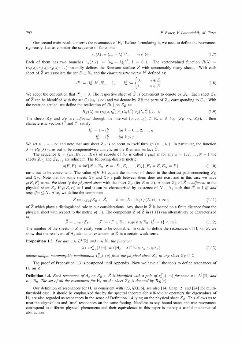
Theorem 1.5. Let the self-adjoint operator Hε, ε ∈ (0, 1), be as in (1.5). Let the sheet ZE ⊂ Z of the Riemannsurface Z be fixed. Define the associated set by:
S(E) :=n ∈ N : (lEn−1, l
En , l
En+1) ∈ (1, 0, 0), (0, 1, 1)
.
Let RE(ε) be as in Definition 1.4 and set R−E(ε) := RE(ε) ∩ C−. Then, the following claims hold:
(i) R−E(ε) ⊂ U(ε) :=λ ∈ C− : |νn−1 − λ||νn − λ| ≤ ε4n2, ∀n ∈ N
.
(ii) For any n ∈ S(E) and sufficiently small ε > 0 there is exactly one resonance λEn (Hε) ∈ C− of Hε on Z−Elying in a neighbourhood of νn, with the expansion
λEn (Hε) = νn −ε4
16
[(2n+ 1) + 2n(n+ 1)i
]+O(ε5), ε→ 0 + . (1.14)
(iii) For any n ∈ N \ S(E) and all sufficiently small ε, r > 0
R−E(ε) ∩ Dr(νn) = ∅.
FIG. 1.1. The region U(0.12) (for ε = 0.12) from Theorem 1.5 (i) (in grey) consists of 6connected components. The components located in the neighbourhoods of the points ν0, ν1, ν2,ν3, are not visible because of being too small. The plot is performed with the aid of Sagemath.
In view of Theorem 1.5 (i) for sufficiently small ε > 0, the resonances of Hε on any sheet of Z are located insome vicinity of the thresholds νn (see Figure 1.1). Such behavior is typical for problems with many thresholds;see e.g. [11, 13] and [14, §2.4, 3.4.2]. Note also that the estimate in Theorem 1.5 (i) reflects the correct order in εin the weak coupling limit ε → 0+ given in Theorem 1.5 (ii). However, the coefficient of ε4 in the definition ofU(ε) can be probably improved. Observe also that R−E(ε) ⊂ U(1) for any ε ∈ (0, 1).
According to Theorem 1.5 (ii)–(iii), the existence of a resonance near the threshold νn, n ∈ N, on a sheet ZEfor small ε > 0 depends only on the branches chosen for rn−1(λ), rn(λ), rn+1(λ) on ZE . Although, one cannotexclude that higher order terms in the asymptotic expansion (1.14) depend on the branches chosen for other squareroots. By exactly the same reason as in Theorem 1.2 (ii), we expect that the error term O(ε5) in Theorem 1.5 (ii)can be replaced by O(ε6). Theorem 1.5 (ii)–(iii) are proven by means of the Birman-Schwinger principle andthe analytic implicit function theorem. The implicit scalar equation on resonances derived in Lemma 4.1 givesanalyticity of ε 7→ λEn (Hε) for small ε > 0 and, as in the bound state case, it can be used to compute further termsin the expansion of λEn (Hε).
We point out that according to numerical tests that we performed, some resonances emerge from the innerpoints of the intervals (νn, νn+1), n ∈ N0, as ε → 1−. The mechanism for the creation of these resonances isunclear at the moment.
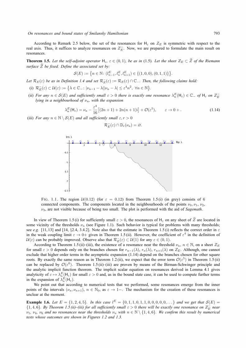
Example 1.6. Let E = 1, 2, 4, 5. In this case lE = 0, 1, 1, 0, 1, 1, 0, 0, 0, 0, 0, . . . and we get that S(E) =1, 4, 6. By Theorem 1.5 (ii)–(iii) for all sufficiently small ε > 0 there will be exactly one resonance on Z−E nearν1, ν4, ν6 and no resonances near the thresholds νn with n ∈ N \ 1, 4, 6. We confirm this result by numericaltests whose outcomes are shown in Figures 1.2 and 1.3.
794 P. Exner, V. Lotoreichik, M. Tater
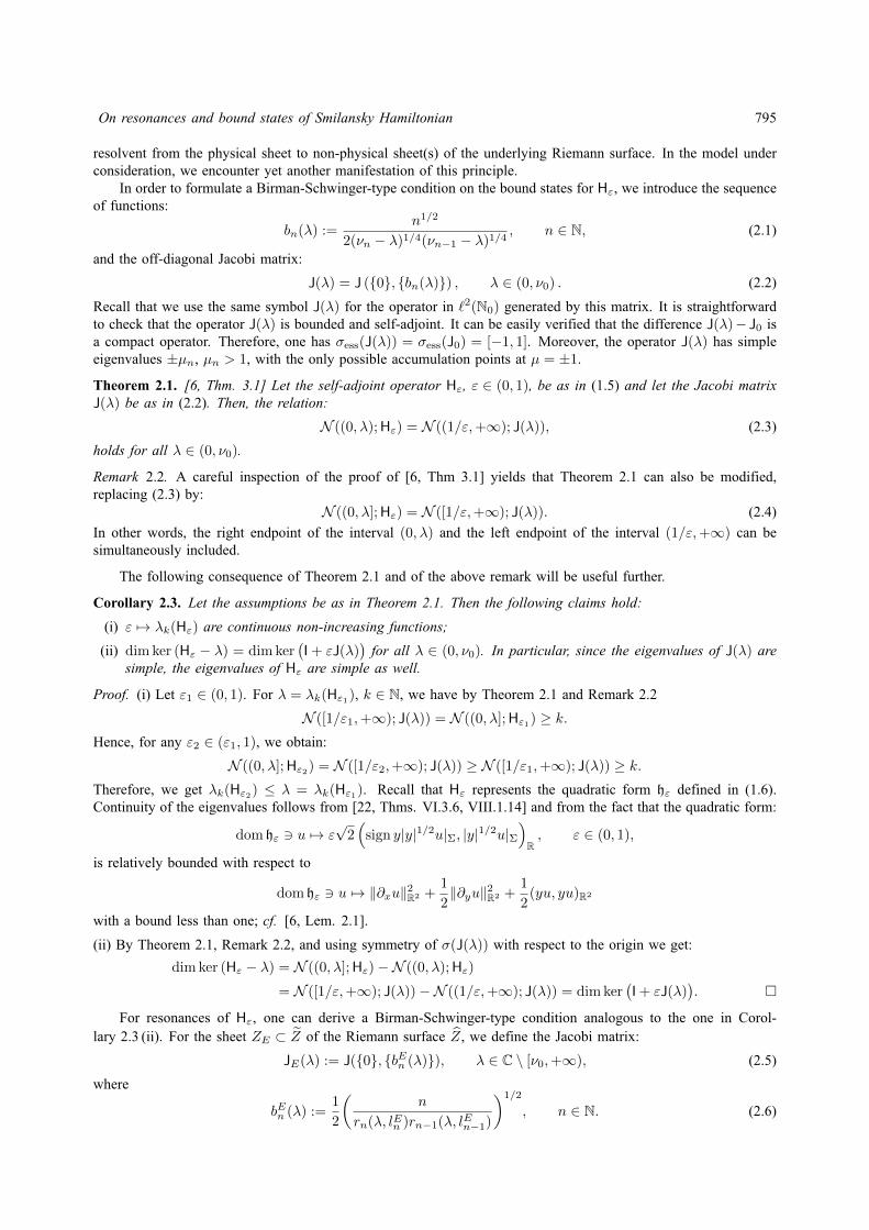
FIG. 1.2. Resonances of Hε with ε = 0.2 lying on Z−E with E = 1, 2, 4, 5 are computednumerically with the help of Mathematica. Unique weakly coupled resonances near the thresholdsν1 = 1.5, ν4 = 4.5, ν6 = 6.5 are located at the intersections of the curves.
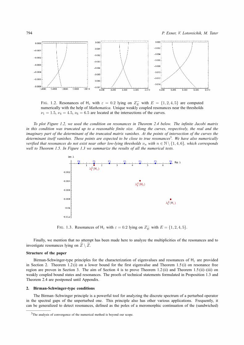
To plot Figure 1.2, we used the condition on resonances in Theorem 2.4 below. The infinite Jacobi matrixin this condition was truncated up to a reasonable finite size. Along the curves, respectively, the real and theimaginary part of the determinant of the truncated matrix vanishes. At the points of intersection of the curves thedeterminant itself vanishes. These points are expected to be close to true resonances3. We have also numericallyverified that resonances do not exist near other low-lying thresholds νn with n ∈ N \ 1, 4, 6, which correspondswell to Theorem 1.5. In Figure 1.3 we summarize the results of all the numerical tests.
FIG. 1.3. Resonances of Hε with ε = 0.2 lying on Z−E with E = 1, 2, 4, 5.
Finally, we mention that no attempt has been made here to analyze the multiplicities of the resonances and toinvestigate resonances lying on Z \ Z.
Structure of the paper
Birman-Schwinger-type principles for the characterization of eigenvalues and resonances of Hε are providedin Section 2. Theorem 1.2 (i) on a lower bound for the first eigenvalue and Theorem 1.5 (i) on resonance freeregion are proven in Section 3. The aim of Section 4 is to prove Theorem 1.2 (ii) and Theorem 1.5 (ii)–(iii) onweakly coupled bound states and resonances. The proofs of technical statements formulated in Proposition 1.3 andTheorem 2.4 are postponed until Appendix.
2. Birman-Schwinger-type conditions
The Birman–Schwinger principle is a powerful tool for analyzing the discrete spectrum of a perturbed operatorin the spectral gaps of the unperturbed one. This principle also has other various applications. Frequently, itcan be generalized to detect resonances, defined as the poles of a meromorphic continuation of the (sandwiched)
3The analysis of convergence of the numerical method is beyond our scope.
On resonances and bound states of Smilansky Hamiltonian 795
resolvent from the physical sheet to non-physical sheet(s) of the underlying Riemann surface. In the model underconsideration, we encounter yet another manifestation of this principle.
In order to formulate a Birman-Schwinger-type condition on the bound states for Hε, we introduce the sequenceof functions:
bn(λ) :=n1/2
2(νn − λ)1/4(νn−1 − λ)1/4, n ∈ N, (2.1)
and the off-diagonal Jacobi matrix:
J(λ) = J (0, bn(λ)) , λ ∈ (0, ν0) . (2.2)
Recall that we use the same symbol J(λ) for the operator in `2(N0) generated by this matrix. It is straightforwardto check that the operator J(λ) is bounded and self-adjoint. It can be easily verified that the difference J(λ)− J0 isa compact operator. Therefore, one has σess(J(λ)) = σess(J0) = [−1, 1]. Moreover, the operator J(λ) has simpleeigenvalues ±µn, µn > 1, with the only possible accumulation points at µ = ±1.
Theorem 2.1. [6, Thm. 3.1] Let the self-adjoint operator Hε, ε ∈ (0, 1), be as in (1.5) and let the Jacobi matrixJ(λ) be as in (2.2). Then, the relation:
N ((0, λ);Hε) = N ((1/ε,+∞); J(λ)), (2.3)
holds for all λ ∈ (0, ν0).
Remark 2.2. A careful inspection of the proof of [6, Thm 3.1] yields that Theorem 2.1 can also be modified,replacing (2.3) by:
N ((0, λ];Hε) = N ([1/ε,+∞); J(λ)). (2.4)
In other words, the right endpoint of the interval (0, λ) and the left endpoint of the interval (1/ε,+∞) can besimultaneously included.
The following consequence of Theorem 2.1 and of the above remark will be useful further.
Corollary 2.3. Let the assumptions be as in Theorem 2.1. Then the following claims hold:
(i) ε 7→ λk(Hε) are continuous non-increasing functions;
(ii) dim ker (Hε − λ) = dim ker(I + εJ(λ)
)for all λ ∈ (0, ν0). In particular, since the eigenvalues of J(λ) are
simple, the eigenvalues of Hε are simple as well.
Proof. (i) Let ε1 ∈ (0, 1). For λ = λk(Hε1), k ∈ N, we have by Theorem 2.1 and Remark 2.2
N ([1/ε1,+∞); J(λ)) = N ((0, λ];Hε1) ≥ k.Hence, for any ε2 ∈ (ε1, 1), we obtain:
N ((0, λ];Hε2) = N ([1/ε2,+∞); J(λ)) ≥ N ([1/ε1,+∞); J(λ)) ≥ k.Therefore, we get λk(Hε2) ≤ λ = λk(Hε1). Recall that Hε represents the quadratic form hε defined in (1.6).Continuity of the eigenvalues follows from [22, Thms. VI.3.6, VIII.1.14] and from the fact that the quadratic form:
dom hε 3 u 7→ ε√
2(
sign y|y|1/2u|Σ, |y|1/2u|Σ)R, ε ∈ (0, 1),
is relatively bounded with respect to
dom hε 3 u 7→ ‖∂xu‖2R2 +1
2‖∂yu‖2R2 +
1
2(yu, yu)R2
with a bound less than one; cf. [6, Lem. 2.1].
(ii) By Theorem 2.1, Remark 2.2, and using symmetry of σ(J(λ)) with respect to the origin we get:
dim ker (Hε − λ) = N ((0, λ];Hε)−N ((0, λ);Hε)
= N ([1/ε,+∞); J(λ))−N ((1/ε,+∞); J(λ)) = dim ker(I + εJ(λ)
).
For resonances of Hε, one can derive a Birman-Schwinger-type condition analogous to the one in Corol-lary 2.3 (ii). For the sheet ZE ⊂ Z of the Riemann surface Z, we define the Jacobi matrix:
JE(λ) := J(0, bEn (λ)), λ ∈ C \ [ν0,+∞), (2.5)
where
bEn (λ) :=1
2
(n
rn(λ, lEn )rn−1(λ, lEn−1)
)1/2
, n ∈ N. (2.6)
796 P. Exner, V. Lotoreichik, M. Tater
The Jacobi matrix JE(λ) in (2.5) is closed, bounded, and everywhere defined in `2(N0), but in general non-selfadjoint. For E = ∅ and λ ∈ (0, ν0) the Jacobi matrix J∅(λ) coincides with J(λ) in (2.2). In what follows it isalso convenient to set bE0 (λ) = 0. In the next theorem, we characterize resonances of Hε lying on the sheet ZE .
Theorem 2.4. Let the self-adjoint operator Hε, ε ∈ (0, 1), be as in (1.5). Let the sheet ZE ⊂ Z be fixed,let RE(ε) be as in Definition 1.4 and the associated operator-valued function JE(λ) be as in (2.5). Then, thefollowing equivalence holds:
λ ∈ RE(ε) ⇐⇒ ker (I + εJE(λ)) 6= 0. (2.7)
For E = ∅, the claim of Theorem 2.4 follows from Corollary 2.3 (ii). The proof of the remaining part ofTheorem 2.4 is postponed until Appendix. The argument essentially relies on Krein-type resolvent formula [7] forHε and on the analytic Fredholm theorem [25, Thm. 3.4.2].
Remark 2.5. Thanks to compactness of the difference JE(λ)−J0 we get by [23, Lem. XIII.4.3] that σess(εJE(λ)) =σess(εJ0)) = [−ε, ε]. Therefore, the equivalence (2.7) can be rewritten as:
λ ∈ RE(ε) ⇐⇒ −1 ∈ σd(εJE(λ)).
Identity JE(λ)∗ = JE(λ) combined with [22, Rem. III.6.23] and with Theorem 2.4 yields that the set RE(ε) issymmetric with respect to the real axis.
3. Localization of bound states and resonances
In this section we prove Theorem 1.2 (i) and Theorem 1.5 (i). The idea of the proof is to estimate the norm ofJE(λ) and to apply Corollary 2.3 (ii) and Theorem 2.4.
Proof of Theorem 1.2 (i) and Theorem 1.5 (i). The square of the norm of the operator JE(λ) in (2.5) can be esti-mated from above by:
‖JE(λ)‖2 ≤ supξ∈`2(N0),‖ξ‖=1
‖JE(λ)ξ‖2 ≤ supξ∈`2(N0),‖ξ‖=1
( ∑n∈N0
|bEn (λ)ξn−1 + bEn+1(λ)ξn+1|2)
≤ supξ∈`2(N0),‖ξ‖=1
(2∑n∈N0
(|bEn (λ)|2|ξn−1|2 + |bEn+1(λ)|2|ξn+1|2
))≤ 4 sup
n∈N0
|bEn (λ)|2 supξ∈`2(N0),‖ξ‖=1
‖ξ‖2 = 4 supn∈N|bEn (λ)|2,
(3.1)
where bEn (λ), n ∈ N0, are defined as in (2.6).If ‖εJE(λ)‖ < 1 holds for a point λ ∈ C−, then the condition ker (I+ εJE(λ)) 6= 0 is not satisfied. Thus, λ
cannot by Theorem 2.4 be a resonance of Hε lying on Z−E in the sense of Definition 1.4. In view of estimate (3.1)and of (2.6) to fulfil ‖εJE(λ)‖ < 1, it suffices to satisfy:
n
|νn−1 − λ|1/2|νn − λ|1/2<
1
ε2, ∀ n ∈ N,
or, equivalently,|νn − λ| · |νn−1 − λ| > ε4n2, ∀ n ∈ N.
Thus, the claim of Theorem 1.5 (i) is proven. If ‖εJ∅(λ)‖ < 1 holds for a point λ ∈ (0, 1/2) then the conditionker (I + εJ∅(λ)) 6= 0 is not satisfied. Thus, by Corollary 2.3 (ii), λ is not an eigenvalue of Hε. In view of (3.1)and (2.6) to fulfil ‖εJ∅(λ)‖ < 1, it suffices to satisfy:(
νn−1 − λ)(νn − λ
)= λ2 − 2nλ+ n2 − 1/4 > n2ε4, ∀ n ∈ N. (3.2)
The roots of the equation λ2 − 2nλ + n2 − 1/4 − n2ε4 = 0 are given by λ±n (ε) = n ±√
1/4 + n2ε4. Sinceλ+n (ε) > 1/2 for all n ∈ N, the condition (3.2) yields λ1(Hε) ≥ min
n∈Nλ−n (ε). For n ∈ N we have:
λ−n+1(ε)− λ−n (ε) = 1− (2n+ 1)ε4(14 + n2ε4
)1/2+(
14 + (n+ 1)2ε4
)1/2 ≥ 1− (2n+ 1)ε4
(2n+ 1)ε2= 1− ε2 > 0.
Hence, minn∈N
λ−n (ε) = λ−1 (ε) and the claim of Theorem 1.2 (i) follows.
On resonances and bound states of Smilansky Hamiltonian 797
4. The weak coupling regime: ε→ 0+
In this section, we prove Theorem 1.2 (ii) and Theorem 1.5 (ii)–(iii). Intermediate results of this section givenin Lemmata 4.1 and 4.3 are of an independent interest.
First, we introduce some auxiliary operators and functions. Let n ∈ N0 and the sheet ZE ⊂ Z be fixed. Wemake use of notation Pkl := en+k−2(·, en+l−2) with k, l ∈ 1, 2, 3. Note that for n = 0 we have Pk1 = P1k = 0for k = 1, 2, 3. It will also be convenient to decompose the Jacobi matrix JE(λ) in (2.5) as:
JE(λ) = Sn,E(λ) + Tn,E(λ), (4.1)
where the operator-valued functions λ 7→ Tn,E(λ),Sn,E(λ) are defined by:
Tn,E(λ) := bEn+1(λ) [P23 + P32] + bEn (λ) [P21 + P12] , Sn,E(λ) := JE(λ)− Tn,E(λ). (4.2)
Clearly, the operator-valued function Sn,E(·) is uniformly bounded on D1/2(νn). Moreover, for sufficientlysmall r = r(n) ∈ (0, 1/2) the bounded operator I + εSn,E(λ) is at the same time boundedly invertible for all(ε, λ) ∈ Ωr(n) := Dr × Dr(νn). Thus, the operator-valued function:
Rn,E(ε, λ) :=(I + εSn,E(λ)
)−1, (4.3)
is well-defined and analytic on Ωr(n) and, in particular, Rn,E(0, νn) = I. Furthermore, we introduce auxiliaryscalar functions Ωr(n) 3 (ε, λ) 7→ fEkl(ε, λ) by:
fEkl(ε, λ) :=(Rn,E(ε, λ)en+k−2, en+l−2
), k, l ∈ 1, 2, 3. (4.4)
Thanks to Rn,E(0, νn) = I we have fEkl(0, νn) = δkl. Finally, we introduce 3× 3 matrix-valued function:
Dr × D×r (νn) 3 (ε, λ) 7→ An,E(ε, λ) :=(aEkl(ε, λ)
)3,3k,l=1
(4.5)
with the entries given for k, l = 1, 2, 3 by:
aEkl(ε, λ) := bEn (λ)(fE1k(ε, λ)δ2l + fE2k(ε, λ)δ1l
)+ bEn+1(λ)
(fE2k(ε, λ)δ3l + fE3k(ε, λ)δ2l
). (4.6)
We remark that rankAn,E(ε, λ) ≤ 2 due to linear dependence between the first and the third columns in An,E(ε, λ).In the first lemma, we derive an implicit scalar equation which characterizes those points λ ∈ C \ [ν0,+∞)
near νn for which the condition ker (I+ εJE(λ)) 6= 0 is satisfied under additional assumption that ε > 0 is smallenough. This equation can be used to characterize the ‘true’ resonances for Hε as well as the weakly coupledbound state if n = 0 and E = ∅.
Lemma 4.1. Let the self-adjoint operator Hε, ε ∈ (0, 1), be as in (1.5). Let n ∈ N0 and the sheet ZE ⊂ Z befixed. Let r = r(n) > 0 be chosen as above. Then for all ε ∈ (0, r) a point λ ∈ Dr(νn) \ [ν0,∞) is a resonanceof Hε on ZE if, and only if
det(I + εAn,E(ε, λ)
)= 0.
Proof. Using the decomposition (4.1) of JE(λ) and the auxiliary operator in (4.3), we find:
dim ker (I + εJE(λ)) = dim ker (I + εSn,E(λ) + εTn,E(λ)) = dim ker (I + εRn,E(ε, λ)Tn,E(λ)) . (4.7)
Note that:rank (Rn,E(ε, λ)Tn,E(λ)) ≤ rank (Tn,E(λ)) ≤ 3
and, hence, using [26, Thm. 3.5 (b)], we get:
dim ker (I + εRn,E(ε, λ)Tn,E(λ)) ≥ 1 ⇐⇒ det (I + εRn,E(ε, λ)Tn,E(λ)) = 0. (4.8)
For the orthogonal projector P := P11 + P22 + P33 the identity Tn,E(λ) = Tn,E(λ)P is straightforward. Hence,employing [27, IV.1.5] we find:
det (I + εRn,E(ε, λ)Tn,E(λ)) = det (I + εRn,E(ε, λ)Tn,E(λ)P) = det (I + εPRn,E(ε, λ)Tn,E(λ)) . (4.9)
For k, l ∈ 1, 2, 3 we can write the following identities:
PkkPRn,E(ε, λ)Tn,E(λ)Pll = PkkRn,E(ε, λ)(bEn (λ) [P21 + P12] + bEn+1(λ) [P23 + P32]
)Pll
= PkkRn,E(ε, λ)(bEn (λ) [P2lδ1l + P1lδ2l] + bEn+1(λ) [P2lδ3l + P3lδ2l]
)= Pklb
En (λ)
[fE2k(ε, λ)δ1l + fE1k(ε, λ)δ2l
]+ Pklb
En+1(λ)
[fE2k(ε, λ)δ3l + fE3k(ε, λ)δ2l
]= aEkl(ε, λ)Pkl
798 P. Exner, V. Lotoreichik, M. Tater
with fEkl as in (4.4), and as a result we get
PRn,E(ε, λ)Tn,E(λ) =
3∑k=1
3∑l=1
aEkl(ε, λ)Pkl,
with aEkl(ε, λ) as in (4.6). Hence, the determinant in (4.9) can be expressed as:
det (I + εRn,E(ε, λ)Tn,E(λ)) = det(I + εAn,E(ε, λ))
where on the right-hand side we have the determinant of the 3× 3 matrix I + εAn,E(ε, λ); cf. (4.5). The claim oflemma then follows from (4.7), (4.8), and Theorem 2.4.
In the second lemma, we establish the existence and investigate properties of solutions of the scalar equation inLemma 4.1. To this aim it is natural to try to apply the analytic implicit function theorem. The main obstacle thatmakes a direct application of the implicit function theorem difficult lies in the fact that λ 7→ det(I+εAn,E(ε, λ)) isnot analytic near νn due to the cut on the real axis. We circumvent this obstacle by applying the analytic implicitfunction theorem to an auxiliary function which is analytic in the disc and has values in different sectors of thisdisc that are in direct correspondence with the values of λ 7→ det(I + εAn,E(ε, λ)) on the four different sheets inZ which are mutually adjacent in a proper way.
Assumption 4.2. Let n ∈ N0 and the sheet ZE ⊂ Z be fixed. Let the sheets ZF , ZG and ZH be such thatZE ∼n−1 ZF , ZF ∼n ZG and ZG ∼n−1 ZH . For r > 0 let the matrix-valued function Dr × D×r 3 (ε, κ) 7→Bn,E(ε, κ) be defined by:
Bn,E(ε, κ) :=
An,E(ε, νn − κ4), arg κ ∈ ΦE := (−π,− 3π
4 ] ∪ (0, π4 ],
An,F (ε, νn − κ4), arg κ ∈ ΦF := (− 3π4 ,−
π2 ] ∪ (π4 ,
π2 ],
An,G(ε, νn − κ4), arg κ ∈ ΦG := (−π2 ,−π4 ] ∪ (π2 ,
3π4 ],
An,H(ε, νn − κ4), arg κ ∈ ΦH := (−π4 , 0] ∪ ( 3π4 , π].
Tracing the changes in the characteristic vector along the path ZE ∼n−1 ZF ∼n ZG ∼n−1 ZH , one easilyverifies that ZH ∼n ZE . Thus, Bn,E is analytic on Dr × D×r for sufficiently small r > 0 which is essentially aconsequence of componentwise analyticity in Dr of vector-valued function:
κ 7→ R•(νn − κ4), • ∈ E,F,G,H for arg κ ∈ Φ•,
where R• is as in (1.9).
Lemma 4.3. Let n ∈ N0 and the sheet ZE ⊂ Z be fixed. Set (p, q, r) := (lEn−1, lEn , l
En+1). Let the matrix-valued
function Bn,E be as in Assumption 4.2. Then the implicit scalar equation:
det(I + εBn,E(ε, κ)
)= 0
has exactly two solutions κn,E,j(·) analytic near ε = 0 such that κn,E,j(0) = 0, satisfyingdet(I + εBn,E(ε, κn,E,j(ε))) = 0 pointwise for sufficiently small ε > 0, and having asymptotic expansions:
κn,E,j(ε) = ε(zn,E)
1/2j
2+O(ε2), ε→ 0+, (4.10)
where zn,E = (−1)q+r(n+ 1) + (−1)p+q+1ni.
Proof. First, we introduce the shorthand notations:
u(κ) := b•n(νn − κ4), v(κ) := b•n+1(νn − κ4), • ∈ E,F,G,H for arg κ ∈ Φ•.
Let bkl with k, l ∈ 1, 2, 3 be the entries of the matrix-valued function Bn,E . Furthermore, we define the scalarfunctions X = X(ε, κ), Y = Y (ε, κ), and Z = Z(ε, κ) by:
X := b11 + b22 + b33,
Y := b11b22 + b22b33 + b11b33 − b13b31 − b12b21 − b23b32,
Z := b11b22b33 + b13b32b21 + b12b23b31 − b13b31b22 − b12b21b33 − b11b23b32.
(4.11)
Employing an elementary formula for the determinant of 3× 3 matrix, the equation det(I + εBn,E(ε, κ)) = 0 canbe equivalently written as:
1 + εX(ε, κ) + ε2Y (ε, κ) + ε3Z(ε, κ) = 0. (4.12)
On resonances and bound states of Smilansky Hamiltonian 799
By a purely algebraic argument, one can derive from (4.6) that Z = 0. Hence, (4.12) simplifies to 1 + εX(ε, κ) +ε2Y (ε, κ) = 0. Introducing new parameter t := ε/κ, we can further rewrite this equation as:
1 + tκX(ε, κ) + t2κ2Y (ε, κ) = 0. (4.13)
Note also that the coefficients (ε, κ) 7→ κX(ε, κ), κ2Y (ε, κ) of the quadratic equation (4.13) are analytic in D2r .
For each fixed pair (ε, κ) the equation (4.13) has (in general) two distinct roots tj(ε, κ), j = 0, 1. The conditiondet(I + εBn,E(ε, κ)) = 0 with κ 6= 0 holds if, and only if at least one of the two conditions:
fj(ε, κ) := ε− κtj(ε, κ) = 0, j = 0, 1, (4.14)
is satisfied. Using analyticity of u(·) and v(·) near κ = 0, we compute:
limκ→0
κu = limr→0+
reiπ/8u(reiπ/8) = limr→0+
n1/2
2
reiπ/8
((−1 + ir4)1/2p (ir4)
1/2q )1/2
=n1/2eiπ/8
2((−1)p+qieiπ/4)1/2,
limκ→0
κv = limr→0+
reiπ/8v(reiπ/8) = limr→0+
(n+ 1)1/2
2
reiπ/8
((ir4)1/2q (1 + ir4)
1/2r )1/2
=(n+ 1)1/2eiπ/8
2((−1)q+reiπ/4)1/2.
Hence, we get:
limε,r→0+
reiπ/8bkl(ε, reiπ/8) = lim
r→0+reiπ/8u(reiπ/8)
(fE2k(0)δ3l + fE3k(0)δ2l
)+ limr→0+
reiπ/8v(reiπ/8)(fE1k(0)δ2l + fE2k(0)δ1l
)=n1/2eiπ/8
(δ2kδ3l + δ3kδ2l
)2((−1)p+qieiπ/4)1/2
+(n+ 1)1/2eiπ/8
(δ1kδ2l + δ2kδ1l
)2((−1)q+reiπ/4)1/2
.
Combining this with (4.11) we end up with:
lim(ε,κ)→0
κX = limε,r→0+
reiπ/8X(ε, reiπ/8) = limε,r→0+
reiπ/8[b11 + b22 + b33
](ε, reiπ/8) = 0,
lim(ε,κ)→0
κ2Y = limε,r→0+
r2eiπ/4Y (ε, reiπ/8)
= limε,r→0+
r2eiπ/4[b11b22 + b22b33 + b11b33 − b13b31 − b12b21 − b23b32
](ε, reiπ/8)
= limε,r→0+
r2eiπ/4[− b12b21 − b23b32
](ε, reiπ/8)
= −(
n1/2eiπ/8
2((−1)p+qieiπ/4)1/2
)2
−(
(n+ 1)1/2eiπ/8
2((−1)q+reiπ/4)1/2
)2
= − (−1)p+q+1ni
4− (−1)q+r(n+ 1)
4= −zn,E
4.
Hence, the roots tj(ε, κ) of (4.13) converge in the limit (ε, κ) → 0 to the roots 2[(zn,E)
1/2j
]−1, j = 0, 1, of the
quadratic equation zn,Et2 − 4 = 0. Moreover, analyticity of the coefficients in equation (4.13), the above limits,
and the formula for the roots of a quadratic equation imply analyticity of the functions (ε, κ) 7→ tj(ε, κ) near 0.
Step 2. The partial derivatives of fj in (4.14) with respect to ε and κ are given by ∂εfj = 1 − κ∂εtj and∂κfj = −tj − κ∂κtj . Analyticity of tj near 0 implies (∂εfj)(0) = 1 and (∂κfj)(0) = −tj . In particular, we haveshown that (∂κfj)(0) 6= 0. Since the functions fj(·) are analytic near 0 and satisfy fj(0) = 0, we can apply theanalytic implicit function theorem [25, Thm. 3.4.2] which yields existence of a unique function κj(·), analytic nearε = 0 such that κj(0) = 0 and that fj(ε, κj(ε)) = 0 holds pointwise. Moreover, the derivative of κj at ε = 0 canbe expressed as:
κ′j(0) = − (∂εfj)(0)
(∂κfj)(0)=
1
tj(0). (4.15)
Hence, we obtain Taylor expansion for κj near ε = 0:
κj(ε) = κj(0) + κ′j(0)ε+O(ε2) =ε
tj(0)+O(ε2) = ε
(zn,E)1/2j
2+O(ε2) ε→ 0 + .
The functions κj , j = 0, 1, satisfy all the requirements in the claim of the lemma.
Now we are prepared to prove Theorem 1.2 (ii) and Theorem 1.5 (ii)–(iii) from the introduction.
800 P. Exner, V. Lotoreichik, M. Tater
Proof of Theorem 1.2 (ii). By Proposition 1.1 (iv) we have N1/2(Hε) = 1 for all sufficiently small ε > 0. Recallthat we denote by λ1(Hε) the corresponding unique eigenvalue. Thus, we have by Lemma 4.1:
det(I + εA0,∅(ε, λ1(Hε))) = 0.
Using the construction of Assumption 4.2 for the physical sheet and n = 0, we obtain
det(I + εB0,∅(ε, (ν0 − λ1(Hε))1/4)) = det(I + εA0,∅(ε, λ1(Hε))) = 0,
where we have chosen the principal branch for (·)1/4. Thus, by Lemma 4.3, we get:
(ν0 − λ1(Hε))1/4 =
ε
2+O(ε2), ε→ 0+,
where we have used the fact that z0,∅ = 1. Hence, taking the fourth power of the left and right hand sides in theabove equation we arrive at:
λ1(Hε) = ν0 −ε4
16+O(ε5), ε→ 0 + .
Proof of Theorem 1.5 (ii)–(iii). Let n ∈ N and the sheet ZE ⊂ Z be fixed. Let us repeat the construction ofAssumption 4.2. By Lemma 4.3 we infer that there exist exactly two analytic solutions κn,E,j , j = 0, 1 of theimplicit scalar equation det(I + εBn,E(ε, κ)) = 0 such that κn,E,j(0) = 0. It can be checked that both solutionscorrespond to the same resonance and it suffices to analyze the solution κn,E := κn,E,0 only.
For all small enough ε > 0 the asymptotics (4.10) yields:
arg(κn,E(ε)) =1
2arg(zn,E) ∈ ΦE , if, and only if n ∈ S(E).
Hence, if n ∈ N \ S(E), Lemmata 4.1 and 4.3 imply that there will be no resonances in the vicinity of the pointλ = νn lying on Z−E for sufficiently small ε > 0. Thus, we have proven Theorem 1.5 (iii). While if n ∈ S(E) weget by Lemmata 4.1 and 4.3 that there will be exactly one resonance
λEn (Hε) = νn − (κn,E(ε))4,
in the vicinity of the point λ = νn lying on Z−E for sufficiently small ε > 0 and its asymptotic expansion is adirect consequence of the asymptotic expansion (4.10) given in Lemma 4.3. Thus, the claim of Theorem 1.5 (ii)follows.
APPENDIX
A. Krein’s formula, meromorphic continuation of resolvent, and condition on resonances
In this appendix, we use Krein’s resolvent formula for Smilansky Hamiltonian to prove Proposition 1.3 andTheorem 2.4 on meromorphic continuation of (Hε − λ)−1 to Z. The proposed continuation procedure is of aniterative nature wherein, we first extend (Hε − λ)−1 to the sheets adjacent to the physical sheet, then to the sheetswhich are adjacent to the sheets being adjacent to the physical sheet and so on.
To this aim, we define for n ∈ N0 the scalar functions C\[ν0,+∞) 7→ yn(λ) and (C\[ν0,+∞))×R 7→ ηn(λ;x)by:
yn(λ) := rn(λ)√νn, ηn(λ;x) := ν1/4
n exp(−rn(λ)|x|), (A.1)
where rn(·), n ∈ N0, is as in (1.7). Next, we introduce the following operator-valued function:
T(λ) : `2(N0)→ H, T(λ)cn := cnηn(λ;x).
For each fixed λ ∈ C \ [ν0,+∞) the operator T(λ) is bounded and everywhere defined and the adjoint of T(λ)acts as:
T(λ)∗un ∼ In(λ;un)n∈N0, In(λ;u) :=
∫R
ηn(λ;x)u(x)dx.
With these preparations, the resolvent difference of Hε and H0 can be expressed by [7, Thm. 6.1] (see also [4, Sec.6]) as follows:
(Hε − λ)−1 = (H0 − λ)−1 + T(λ)Y(λ)[(I + εJ∅(λ)
)−1 − I]Y(λ)T(λ)∗, λ ∈ C \ [ν0,+∞), (A.2)
where H0 is the Smilansky Hamiltonian with ε = 0, Y(λ) = diag(2yn(λ))−1/2 and J∅(λ) is as in (2.5). Theformula (A.2) can be viewed as a particular case of abstract Krein’s formula (see e.g. [29–31]) for the resolventdifference of two self-adjoint extensions of their common densely defined symmetric restriction.
On resonances and bound states of Smilansky Hamiltonian 801
Proof of Proposition 1.3 and Theorem 2.4. Let us fix n ∈ N0 and a sheet ZE ⊂ Z. We denote by Rn(λ) theresolvent of the self-adjoint operator H2(R) 3 f 7→ −f ′′ + νnf in the Hilbert space L2(R). We can express thefunction r∅n,ε(·;u) in (1.13) using Krein’s formula (A.2) as:
r∅n,ε(λ;u) =⟨(Hε − λ)−1u⊗ en, u⊗ en
⟩=⟨(H0 − λ)−1u⊗ en, u⊗ en
⟩+(Y(λ)
[(I + εJ∅(λ))
−1 − I]Y(λ)T(λ)∗u⊗ en,T(λ)∗u⊗ en
)= (Rn(λ)u, u)R + In(λ;u)In(λ;u)
([(I + εJ∅(λ))
−1 − I]Y(λ)en,Y(λ)∗en
)= (Rn(λ)u, u)R +
In(λ;u)In(λ;u)
2yn(λ)
[((I + εJ∅(λ)
)−1en, en
)− 1
].
Since (Rn(λ)u, u)R, yn(λ), In(λ;u), and In(λ;u) can be easily analytically continued to Z, to extend r∅n,ε(·;u)
meromorphically to the other sheets of the component Z it suffices to extend:
s∅n,ε(λ) :=(
(I + εJ∅(λ))−1 en, en
),
meromorphically from Z∅ to Z. The poles of the meromorphic extension of s∅n,ε(·) can be identified with theresonances of Hε in the sense of Definition 1.4.
To this aim, we set by definition:
sEn,ε(λ) :=(
(I + εJE(λ))−1 en, en
),
for any λ ∈ C \ [ν0,+∞) such that −1 /∈ σ(εJE(λ)). In what follows, we let ZE and ZF be two sheets of Z suchthat ZE ∼n−1 ZF with n ∈ N0
4. Suppose that λ 7→ sEn,ε(·) is well defined and meromorphic either on Z+E or on
Z−E . Next, we extend λ 7→ sEn,ε(·) meromorphically from Z±E to Z∓F . Without loss of generality, we restrict ourattention to the case that λ 7→ sEn,ε(·) is meromorphic on Z+
E and extend it meromorphically to Z−F . On the openset Ωn := C+ ∪ C− ∪ (νn−1, νn), the operator-valued function:
JEF (λ) :=
JE(λ), λ ∈ C+,
JF (λ), λ ∈ Ωn \ C+,
is analytic which is essentially a consequence of analyticity on Ωn of the entries b•m(λ) (with • = E for λ ∈ C+
and • = F for λ ∈ C−) for the underlying Jacobi matrix. Thus, the operator-valued function:
Ωn 3 λ 7→ AEFε (λ) := ε (I + εJ0)−1
(JEF (λ)− J0)
is also analytic on Ωn because of the analyticity of JEF (λ). Furthermore, the values of AEFε (·) are compactoperators thanks to compactness of the difference JEF (λ)− J0. Taking into account that:((
I + AEFε (λ))−1
en, (I + εJ0)−1 en
)=
sEn,ε(λ), λ ∈ C+,
sFn,ε(λ), λ ∈ Ωn \ C+,
we obtain from the analytic Fredholm theorem [28, Thm. VI.14] that C− 3 λ 7→ sFn,ε(λ) is a meromorphiccontinuation of C+ 3 λ 7→ sEn,ε(λ) across the interval (νn−1, νn) and that the poles of C− 3 λ 7→ sFn,ε(λ) satisfythe condition:
ker (I + εJF (λ)) 6= 0, λ ∈ C−.
Starting from the physical sheet Z∅, we use the above procedure iteratively to extend s∅n,ε(·) meromorphically to
the whole of Z thus proving Proposition 1.3 and Theorem 2.4.
Acknowledgements
This research was supported by the Czech Science Foundation (GACR) within the project 14-06818S.
4Recall that for any sheet ZE holds ZE ∼−1 ZE .
802 P. Exner, V. Lotoreichik, M. Tater
References
[1] Smilansky U. Irreversible quantum graphs. Waves Random Media, 2004, 14 (1), S143–S153.[2] Evans W. D., Solomyak M. Smilansky’s model of irreversible quantum graphs. I: The absolutely continuous spectrum. J. Phys. A: Math.
Gen., 2005, 38 (21), P. 4611–4627.[3] Evans W. D., Solomyak M. Smilansky’s model of irreversible quantum graphs. II: The point spectrum. J. Phys. A: Math. Gen., 2005, 38
(35), P. 7661–7675.[4] Naboko S., Solomyak M. On the absolutely continuous spectrum in a model of an irreversible quantum graph. Proc. Lond. Math. Soc.
(3), 2006, 92 (1), P. 251–272.[5] Rozenblum G., Solomyak M. On a family of differential operators with the coupling parameter in the boundary condition. J. Comput.
Appl. Math., 2007, 208 (1), P. 57–71.[6] Solomyak M. On the discrete spectrum of a family of differential operators. Funct. Anal. Appl., 2004, 38 (3), P. 217–223.[7] Solomyak M. On a mathematical model of irreversible quantum graphs. St. Petersburg Math. J., 2006, 17 (5), P. 835–864.[8] Solomyak M. On the limiting behaviour of the spectra of a family of differential operators. J. Phys. A: Math. Gen., 2006, 39 (33),
P. 10477–10489.[9] Guarneri I. Irreversible behaviour and collapse of wave packets in a quantum system with point interactions. J. Phys. A: Math. Theor.,
2011, 44 (48), 485304, 22 p.[10] Aslanyan A., Parnovski L., and Vassiliev D. Complex resonances in acoustic waveguides. Q. J. Mech. Appl. Math., 2000, 53 (3),
P. 429–447.[11] Duclos P., Exner P., Meller B. Open quantum dots: Resonances from perturbed symmetry and bound states in strong magnetic fields. Rep.
Math. Phys., 2001, 47 (2), P. 253–267.[12] Edward J. On the resonances of the Laplacian on waveguides. J. Math. Anal. Appl., 2002, 272 (1), P. 89–116.[13] Exner P., Gawlista R., Seba P., Tater M. Point interactions in a strip. Ann. Phys., 1996, 252 (1), P. 133–179.[14] Exner P., Kovarık H. Quantum waveguides. Springer, Cham., 2015, 382 p.[15] Christiansen T. Some upper bounds on the number of resonances for manifolds with infinite cylindrical ends. Ann. Henri Poincare, 2002,
3 (5), P. 895–920.[16] Christiansen T. Asymptotics for a resonance-counting function for potential scattering on cylinders. J. Funct. Anal., 2004, 216 (1),
P. 172–190.[17] Barseghyan D., Exner P. Spectral estimates for a class of Schrodinger operators with infinite phase space and potential unbounded from
below. J. Phys. A: Math. Theor., 2012, 45 (7), 075204, 14 p.[18] Barseghyan D., Exner P. A regular version of Smilansky model. J. Math. Phys., 2014, 55 (4), 042104, 13 p.[19] Barseghyan D., Exner P., Khrabustovskyi A., and Tater M. Spectral analysis of a class of Schrodinger operators exhibiting a parameter-
dependent spectral transition. J. Phys. A: Math. Theor., 2016, 49 (16), 165302.[20] Abramowitz M., Stegun I. Handbook of Mathematical Functions with Formulas, Graphs, and Mathematical Tables, U.S. Government
Printing Office, Washington, D.C:, 1964. 1046 p.[21] Chihara T. An introduction to orthogonal polynomials. Gordon and Breach Science Publishers, New York-London-Paris., 1978, 249 p.[22] Kato T. Perturbation theory for linear operators. Springer-Verlag, Berlin, 1995, 619 p.[23] Reed M., Simon B. Methods of modern mathematical physics. IV. Analysis of operators. Academic Press, New York, 1978, 396 p.[24] Motovilov A. Analytic continuation of S matrix in multichannel problems. Theoret. Math. Phys., 1993, 95 (3), P. 692–699.[25] Simon B. Basic complex analysis. A comprehensive course in analysis, part 2A. American Mathematical Society, Providence, 2015, 641 p.[26] Simon B. Trace ideals and their applications. 2nd ed. American Mathematical Society, Providence, 2005, 150 p.[27] Gohberg I. C., Krein M. G. Introduction to the theory of linear nonselfadjoint operators. Translations of Mathematical Monographs,
American Mathematical Society, Providence, RI, 1969, 378 p.[28] Reed M., Simon B. Methods of modern mathematical physics. I: Functional analysis. Academic Press, New York, 1980, 400 p.[29] Behrndt J., Langer M. Elliptic operators, Dirichlet-to-Neumann maps and quasi boundary triples. in: Operator Methods for Boundary
Value Problems, London Math. Soc. Lecture Note Series, 2012, 404, P. 121–160.[30] Bruning J., Geyler V., Pankrashkin K. Spectra of self-adjoint extensions and applications to solvable Schrodinger operators. Rev. Math.
Phys., 2008, 20 (1), P. 1–70.[31] Derkach V., Malamud M. Generalized resolvents and the boundary value problems for Hermitian operators with gaps. J. Funct. Anal.,
1991, 95 (1), P. 1–95.
NANOSYSTEMS: PHYSICS, CHEMISTRY, MATHEMATICS, 2016, 7 (5), P. 803–815
Spectral properties of a symmetric three-dimensional quantum dot with a pairof identical attractive δ-impurities symmetrically situated around the origin II
S. Albeverio1,2,3, S. Fassari2,4, and F. Rinaldi2,4
1Institut fur Angewandte Mathematik, HCM, IZKS, BiBoS, Universitat Bonn, Endenicheralee 60,D-53115 Bonn, Germany
2CERFIM, PO Box 1132, CH-6601 Locarno, Switzerland3Chair Professorship, Department of Mathematics and Statistics,King Fahd University of Petroleum and Minerals, Dhahran, KSA
4Universita degli Studi Guglielmo Marconi, Via Plinio 44, I-00193 Rome, Italy
PACS 02.30.Gp, 02.30.Hq, 02.30.Hq, 02.30.Lt, 02.30.Sa, 02.30.Tb, 03.65.Db, 03.65.Ge, 68.65.Hb
DOI 10.17586/2220-8054-2016-7-5-803-815
In this note, we continue our analysis (started in [1]) of the isotropic three-dimensional harmonic oscillator perturbed by a pair of identical
attractive point interactions symmetrically situated with respect to the origin, that is to say, the mathematical model describing a symmetric
quantum dot with a pair of point impurities. In particular, by making the coupling constant (to be renormalized) dependent also upon the
separation distance between the two impurities, we prove that it is possible to rigorously define the unique self-adjoint Hamiltonian that,
differently from the one introduced in [1], behaves smoothly as the separation distance between the impurities shrinks to zero. In fact, we
rigorously prove that the Hamiltonian introduced in this note converges in the norm-resolvent sense to that of the isotropic three-dimensional
harmonic oscillator perturbed by a single attractive point interaction situated at the origin having double strength, thus making this three-
dimensional model more similar to its one-dimensional analog (not requiring the renormalization procedure) as well as to the three-dimensional
model involving impurities given by potentials whose range may even be physically very short but different from zero. Moreover, we show
the manifestation of the Zeldovich effect, known also as level rearrangement, in the model investigated herewith. More precisely, we take
advantage of our renormalization procedure to demonstrate the possibility of using the concept of ‘Zeldovich spiral’, introduced in the case of
perturbations given by rapidly decaying potentials, also in the case of point perturbations.
Keywords: level crossing, degeneracy, point interactions, renormalisation, Schrodinger operators, quantum dots, perturbed quantum oscillators,
Zeldovich effect, level rearrangement.
Received: 27 June 2016
Revised: 25 July 2016
1. Introduction
The main purpose of this note is to extend the results of [1] by fixing the problematic behavior of theHamiltonian Hβ,~x0 studied therein in the limit x0 = | ± ~x0| → 0+, that is to say as the distance between the twotwin point perturbations shrinks to zero. As was noticed in [1], the Hamiltonian Hβ,~x0, the self-adjoint energyoperator of the three-dimensional isotropic harmonic oscillator perturbed by a pair of identical point interactionssymmetrically situated around the origin defined rigorously by means of a ’coupling constant renormalization’, doesnot converge to H2β , the one of the three-dimensional isotropic harmonic oscillator perturbed by a single pointinteraction situated at the origin having double strength. Such a singular behavior manifested by singular doublewells with point interactions in three dimensions is in sharp contrast with conventional double wells generatedby potentials, whose range may even be very short but non-zero. By citing [1] it is important to recall that’as is well known to Quantum Chemistry students, three-dimensional interactions with a nonzero range do notmanifest this singular behavior in the limit of the distance between the two centers shrinking to zero, as theclassical textbook example of H+
2 smoothly approaching He+ in the limit R → 0+ clearly shows’ (see [2–4]).The same phenomenon had been observed in [5] (see also [6–10]) dealing with another model involving a pairof identical point interactions symmetrically situated around the origin defined rigorously by using a ’couplingconstant renormalization’ as well, namely the one-dimensional energy operator in which the kinetic component isgiven by the Salpeter free Hamiltonian
√p2 +m2, m > 0.
As was fully proved in [10], this singular behavior does not occur in the one-dimensional analog of the modelgiven that the Dirac distribution is an infinitesimally small perturbation of the Laplacian in one dimension, which
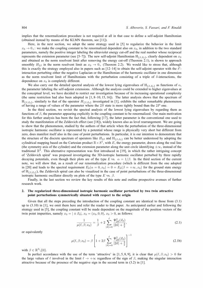
804 S. Albeverio, S. Fassari, and F. Rinaldi
implies that the renormalization procedure is not required at all in that case to define a self-adjoint Hamiltonian(obtained instead by means of the KLMN theorem, see [11]).
Here, in the next section, we adopt the same strategy used in [5] to regularize the behavior in the limitx0 → 0+: we make the coupling constant to be renormalized dependent also on x0, in addition to the two standardparameters, namely the positive integer labeling the ultraviolet energy cut-off and the real number whose reciprocalrepresents the extension parameter (see [5–7]). The new self-adjoint Hamiltonian Hβ,~x0, clearly dependent on x0and obtained as the norm resolvent limit after removing the energy cut-off (Theorem 2.1), is shown to approachsmoothly H2β in the norm resolvent limit as x0 → 0+ (Theorem 2.2). We would like to stress that, althoughthis is exactly the strategy employed also in papers such as [12–14] to obtain the self-adjoint operator with the δ′-interaction perturbing either the negative Laplacian or the Hamiltonian of the harmonic oscillator in one dimensionas the norm resolvent limit of Hamiltonians with the perturbation consisting of a triple of δ-interactions, thedependence on x0 is completely different.
We also carry out the detailed spectral analysis of the lowest lying eigenvalues of Hβ,~x0 as functions of α,the parameter labeling the self-adjoint extensions. Although the analysis could be extended to higher eigenvalues atthe conceptual level, we have decided to restrict our investigation because of its increasing operational complexity(the same restriction had also been adopted in [1, 8–10, 15, 16]). The latter analysis shows that the spectrum ofHβ,~x0, similarly to that of the operator Hβ,~x0 investigated in [1], exhibits the rather remarkable phenomenonof having a range of values of the parameter where the 2S state is more tightly bound than the 2P one.
In the third section, we revisit the spectral analysis of the lowest lying eigenvalues by regarding them asfunctions of β, the parameter appearing explicitly in the coupling constant to be renormalized. Our main motivationfor this further analysis has been the fact that, following [17], the latter parameter is the conventional one used tostudy the manifestation of the Zeldovich effect (see [18]), widely known also as level rearrangement. We are goingto show that the phenomenon, studied by the authors of that article when the perturbation of the three-dimensionalisotropic harmonic oscillator is represented by a potential whose range is physically very short but different fromzero, does manifest itself also in the case of point perturbations. In particular, it is our intention to demonstrate thatthe structure of the discrete spectrum of operators like H2β and Hβ,~x0 can be better understood by adopting thecylindrical mapping based on the Cartesian product R×S1, with E, the energy parameter, drawn along the real line(the symmetry axis of the cylinder) and the extension parameter along the unit circle identifying ±∞, instead of thetraditional R2. This alternative representation was first introduced in [19], in which the rather intriguing conceptof ‘Zeldovich spiral’ was proposed investigating the 3D-isotropic harmonic oscillator perturbed by three rapidlydecaying potentials, even though their plots are of the type E vs. α = 1/β. In the third section of the currentnote, we will show that, as a result of our renormalization procedure (which is different from the one adoptedin [20] and leads to the spectral requirement E0(α = 0, x0) = 0 = E0(β = +∞, x0) for the ground state energyof Hβ,~x0), the Zeldovich spiral can also be visualized in the case of point perturbations of the three-dimensionalisotropic harmonic oscillator directly on plots of the type E vs. β.
Finally, in the last section we review the key results of this note and outline prospective avenues of furtherresearch work.
2. The regularized three-dimensional isotropic harmonic oscillator perturbed by two twin attractivepoint perturbations symmetrically situated with respect to the origin
Given that all the steps preceding the introduction of the coupling constant are identical to those from (3.1)up to (3.10) in [1], we omit them here and refer the reader to that paper. As anticipated earlier and following thestrategy used in [5], the coupling constant will be made dependent on the magnitude of the position vectors of thetwin point impurities, namely x0 = | ± ~x0|, x0 = (x0, 0, 0), x0 > 0, as follows:
1
µ(`, β;x0)=
1
β+ 2
∑|~n|=0
Ψ22~n(~x0)
|2~n|+ 32
, (2.1)
or equivalently
µ(`, β;x0) = β
1 + 2β∑|~n|=0
Ψ22~n(~x0)
|2~n|+ 32
−1 (2.1b)
with β ∈ R3\0.In perfect accordance with the use of the term ‘attractive’ in [1, 5, 8, 9], it is clear that µ(`, β;x0) > 0 for
the large values of ` involved in the limit ` → +∞ regardless of the sign of β, making the singular interactionattractive because of the presence of the negative sign in the second term in (3.2) in [1].
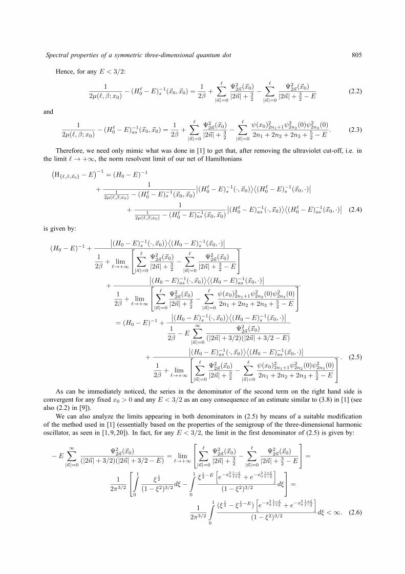
Spectral properties of a symmetric three-dimensional quantum dot 805
Hence, for any E < 3/2:
1
2µ(`, β;x0)− (H`
0 − E)−1s (~x0, ~x0) =1
2β+∑|~n|=0
Ψ22~n(~x0)
|2~n|+ 32
−∑|~n|=0
Ψ22~n(~x0)
|2~n|+ 32 − E
(2.2)
and
1
2µ(`, β;x0)− (H`
0 − E)−1as (~x0, ~x0) =1
2β+∑|~n|=0
Ψ22~n(~x0)
|2~n|+ 32
−∑|~n|=0
ψ(x0)22n1+1ψ22n2
(0)ψ22n3
(0)
2n1 + 2n2 + 2n3 + 52 − E
. (2.3)
Therefore, we need only mimic what was done in [1] to get that, after removing the ultraviolet cut-off, i.e. inthe limit `→ +∞, the norm resolvent limit of our net of Hamiltonians(
H`,β,~x0 − E)−1
= (H0 − E)−1
+1
12µ(`,β;x0)
− (H`0 − E)−1s (~x0, ~x0)
∣∣(H`0 − E)−1s (·, ~x0)
⟩⟨(H`
0 − E)−1s (~x0, ·)∣∣
+1
12µ(`,β;x0)
− (H`0 − E)−1as (~x0, ~x0)
∣∣(H`0 − E)−1as (·, ~x0)
⟩⟨(H`
0 − E)−1as (~x0, ·)∣∣ (2.4)
is given by:
(H0 − E)−1 +
∣∣(H0 − E)−1s (·, ~x0)⟩⟨
(H0 − E)−1s (~x0, ·)∣∣
1
2β+ lim`→+∞
∑|~n|=0
Ψ22~n(~x0)
|2~n|+ 32
−∑|~n|=0
Ψ22~n(~x0)
|2~n|+ 32 − E
+
∣∣(H0 − E)−1as (·, ~x0)⟩⟨
(H0 − E)−1as (~x0, ·)∣∣
1
2β+ lim`→+∞
∑|~n|=0
Ψ22~n(~x0)
|2~n|+ 32
−∑|~n|=0
ψ(x0)22n1+1ψ22n2
(0)ψ22n3
(0)
2n1 + 2n2 + 2n3 + 52 − E
= (H0 − E)−1 +
∣∣(H0 − E)−1s (·, ~x0)⟩⟨
(H0 − E)−1s (~x0, ·)∣∣
1
2β− E
∞∑|~n|=0
Ψ22~n(~x0)
(|2~n|+ 3/2)(|2~n|+ 3/2− E)
+
∣∣(H0 − E)−1as (·, ~x0)⟩⟨
(H0 − E)−1as (~x0, ·)∣∣
1
2β+ lim`→+∞
∑|~n|=0
Ψ22~n(~x0)
|2~n|+ 32
−∑|~n|=0
ψ(x0)22n1+1ψ22n2
(0)ψ22n3
(0)
2n1 + 2n2 + 2n3 + 52 − E
. (2.5)
As can be immediately noticed, the series in the denominator of the second term on the right hand side isconvergent for any fixed x0 > 0 and any E < 3/2 as an easy consequence of an estimate similar to (3.8) in [1] (seealso (2.2) in [9]).
We can also analyze the limits appearing in both denominators in (2.5) by means of a suitable modificationof the method used in [1] (essentially based on the properties of the semigroup of the three-dimensional harmonicoscillator, as seen in [1, 9, 20]). In fact, for any E < 3/2, the limit in the first denominator of (2.5) is given by:
− E∞∑|~n|=0
Ψ22~n(~x0)
(|2~n|+ 3/2)(|2~n|+ 3/2− E)= lim`→+∞
∑|~n|=0
Ψ22~n(~x0)
|2~n|+ 32
−∑|~n|=0
Ψ22~n(~x0)
|2~n|+ 32 − E
=
1
2π3/2
1∫0
ξ12
(1− ξ2)3/2dξ −
1∫0
ξ12−E
[e−x
20
1−ξ1+ξ + e−x
20
1+ξ1−ξ
](1− ξ2)3/2
dξ
=
1
2π3/2
1∫0
(ξ12 − ξ 1
2−E)[e−x
20
1−ξ1+ξ + e−x
20
1+ξ1−ξ
](1− ξ2)3/2
dξ <∞. (2.6)
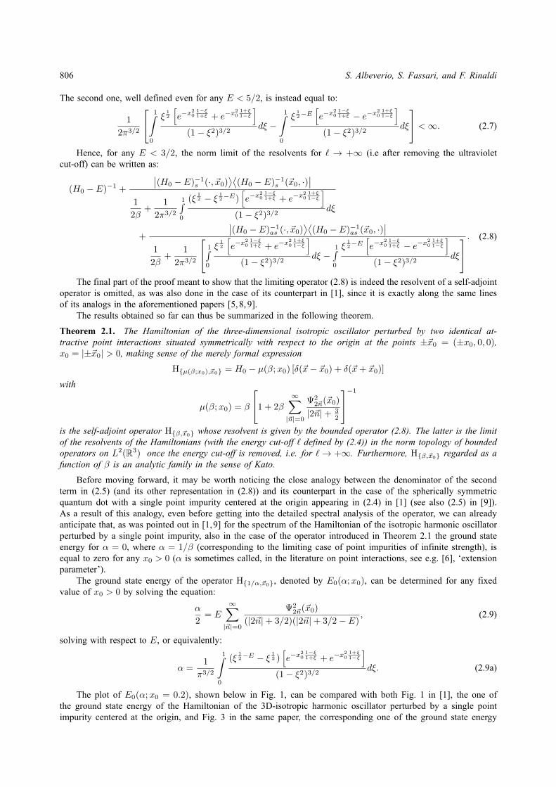
806 S. Albeverio, S. Fassari, and F. Rinaldi
The second one, well defined even for any E < 5/2, is instead equal to:
1
2π3/2
1∫0
ξ12
[e−x
20
1−ξ1+ξ + e−x
20
1+ξ1−ξ
](1− ξ2)3/2
dξ −1∫
0
ξ12−E
[e−x
20
1−ξ1+ξ − e−x
20
1+ξ1−ξ
](1− ξ2)3/2
dξ
<∞. (2.7)
Hence, for any E < 3/2, the norm limit of the resolvents for ` → +∞ (i.e after removing the ultravioletcut-off) can be written as:
(H0 − E)−1 +
∣∣(H0 − E)−1s (·, ~x0)⟩⟨
(H0 − E)−1s (~x0, ·)∣∣
1
2β+
1
2π3/2
1∫0
(ξ12 − ξ 1
2−E)[e−x
20
1−ξ1+ξ + e−x
20
1+ξ1−ξ
](1− ξ2)3/2
dξ
+
∣∣(H0 − E)−1as (·, ~x0)⟩⟨
(H0 − E)−1as (~x0, ·)∣∣
1
2β+
1
2π3/2
1∫0
ξ12
[e−x
20
1−ξ1+ξ + e−x
20
1+ξ1−ξ
](1− ξ2)3/2
dξ −1∫0
ξ12−E
[e−x
20
1−ξ1+ξ − e−x
20
1+ξ1−ξ
](1− ξ2)3/2
dξ
. (2.8)
The final part of the proof meant to show that the limiting operator (2.8) is indeed the resolvent of a self-adjointoperator is omitted, as was also done in the case of its counterpart in [1], since it is exactly along the same linesof its analogs in the aforementioned papers [5, 8, 9].
The results obtained so far can thus be summarized in the following theorem.
Theorem 2.1. The Hamiltonian of the three-dimensional isotropic oscillator perturbed by two identical at-tractive point interactions situated symmetrically with respect to the origin at the points ±~x0 = (±x0, 0, 0),x0 = |±~x0| > 0, making sense of the merely formal expression
Hµ(β;x0),~x0 = H0 − µ(β;x0) [δ(~x− ~x0) + δ(~x+ ~x0)]
with
µ(β;x0) = β
1 + 2β
∞∑|~n|=0
Ψ22~n(~x0)
|2~n|+ 32
−1is the self-adjoint operator Hβ,~x0 whose resolvent is given by the bounded operator (2.8). The latter is the limitof the resolvents of the Hamiltonians (with the energy cut-off ` defined by (2.4)) in the norm topology of boundedoperators on L2(R3) once the energy cut-off is removed, i.e. for `→ +∞. Furthermore, Hβ,~x0 regarded as afunction of β is an analytic family in the sense of Kato.
Before moving forward, it may be worth noticing the close analogy between the denominator of the secondterm in (2.5) (and its other representation in (2.8)) and its counterpart in the case of the spherically symmetricquantum dot with a single point impurity centered at the origin appearing in (2.4) in [1] (see also (2.5) in [9]).As a result of this analogy, even before getting into the detailed spectral analysis of the operator, we can alreadyanticipate that, as was pointed out in [1,9] for the spectrum of the Hamiltonian of the isotropic harmonic oscillatorperturbed by a single point impurity, also in the case of the operator introduced in Theorem 2.1 the ground stateenergy for α = 0, where α = 1/β (corresponding to the limiting case of point impurities of infinite strength), isequal to zero for any x0 > 0 (α is sometimes called, in the literature on point interactions, see e.g. [6], ‘extensionparameter’).
The ground state energy of the operator H1/α,~x0, denoted by E0(α;x0), can be determined for any fixedvalue of x0 > 0 by solving the equation:
α
2= E
∞∑|~n|=0
Ψ22~n(~x0)
(|2~n|+ 3/2)(|2~n|+ 3/2− E), (2.9)
solving with respect to E, or equivalently:
α =1
π3/2
1∫0
(ξ12−E − ξ 1
2 )[e−x
20
1−ξ1+ξ + e−x
20
1+ξ1−ξ
](1− ξ2)3/2
dξ. (2.9a)
The plot of E0(α;x0 = 0.2), shown below in Fig. 1, can be compared with both Fig. 1 in [1], the one ofthe ground state energy of the Hamiltonian of the 3D-isotropic harmonic oscillator perturbed by a single pointimpurity centered at the origin, and Fig. 3 in the same paper, the corresponding one of the ground state energy
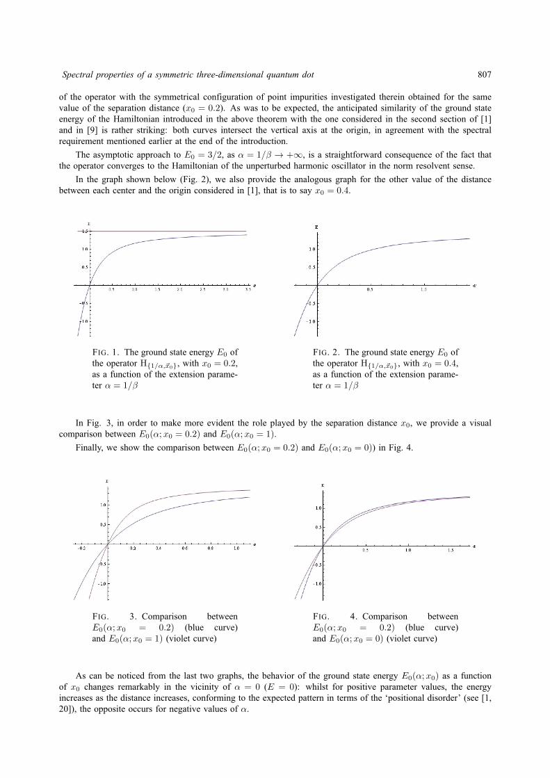
Spectral properties of a symmetric three-dimensional quantum dot 807
of the operator with the symmetrical configuration of point impurities investigated therein obtained for the samevalue of the separation distance (x0 = 0.2). As was to be expected, the anticipated similarity of the ground stateenergy of the Hamiltonian introduced in the above theorem with the one considered in the second section of [1]and in [9] is rather striking: both curves intersect the vertical axis at the origin, in agreement with the spectralrequirement mentioned earlier at the end of the introduction.
The asymptotic approach to E0 = 3/2, as α = 1/β → +∞, is a straightforward consequence of the fact thatthe operator converges to the Hamiltonian of the unperturbed harmonic oscillator in the norm resolvent sense.
In the graph shown below (Fig. 2), we also provide the analogous graph for the other value of the distancebetween each center and the origin considered in [1], that is to say x0 = 0.4.
FIG. 1. The ground state energy E0 ofthe operator H1/α,~x0, with x0 = 0.2,as a function of the extension parame-ter α = 1/β
FIG. 2. The ground state energy E0 ofthe operator H1/α,~x0, with x0 = 0.4,as a function of the extension parame-ter α = 1/β
In Fig. 3, in order to make more evident the role played by the separation distance x0, we provide a visualcomparison between E0(α;x0 = 0.2) and E0(α;x0 = 1).
Finally, we show the comparison between E0(α;x0 = 0.2) and E0(α;x0 = 0)) in Fig. 4.
FIG. 3. Comparison betweenE0(α;x0 = 0.2) (blue curve)and E0(α;x0 = 1) (violet curve)
FIG. 4. Comparison betweenE0(α;x0 = 0.2) (blue curve)and E0(α;x0 = 0) (violet curve)
As can be noticed from the last two graphs, the behavior of the ground state energy E0(α;x0) as a functionof x0 changes remarkably in the vicinity of α = 0 (E = 0): whilst for positive parameter values, the energyincreases as the distance increases, conforming to the expected pattern in terms of the ‘positional disorder’ (see [1,20]), the opposite occurs for negative values of α.
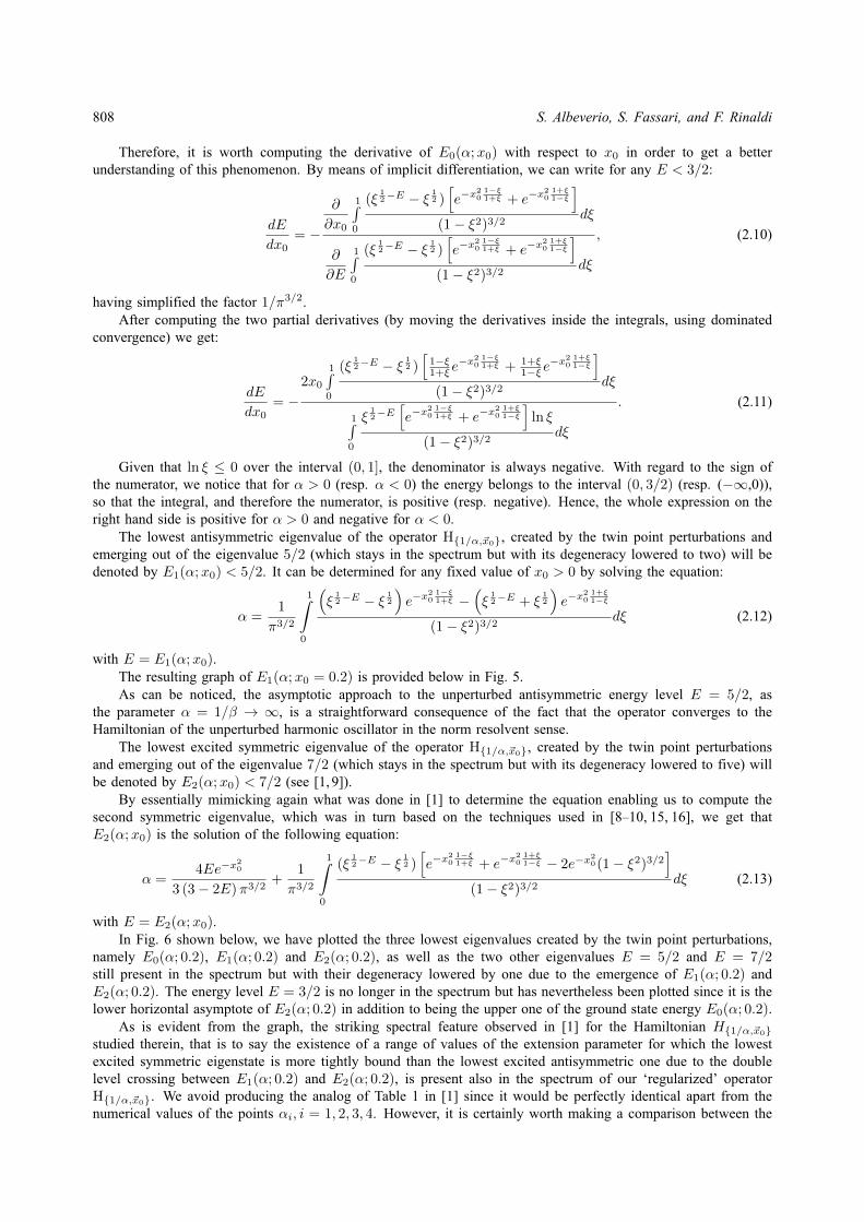
808 S. Albeverio, S. Fassari, and F. Rinaldi
Therefore, it is worth computing the derivative of E0(α;x0) with respect to x0 in order to get a betterunderstanding of this phenomenon. By means of implicit differentiation, we can write for any E < 3/2:
dE
dx0= −
∂
∂x0
1∫0
(ξ12−E − ξ 1
2 )[e−x
20
1−ξ1+ξ + e−x
20
1+ξ1−ξ
](1− ξ2)3/2
dξ
∂
∂E
1∫0
(ξ12−E − ξ 1
2 )[e−x
20
1−ξ1+ξ + e−x
20
1+ξ1−ξ
](1− ξ2)3/2
dξ
, (2.10)
having simplified the factor 1/π3/2.After computing the two partial derivatives (by moving the derivatives inside the integrals, using dominated
convergence) we get:
dE
dx0= −
2x01∫0
(ξ12−E − ξ 1
2 )[1−ξ1+ξ e
−x20
1−ξ1+ξ + 1+ξ
1−ξ e−x2
01+ξ1−ξ
](1− ξ2)3/2
dξ
1∫0
ξ12−E
[e−x
20
1−ξ1+ξ + e−x
20
1+ξ1−ξ
]ln ξ
(1− ξ2)3/2dξ
. (2.11)
Given that ln ξ ≤ 0 over the interval (0, 1], the denominator is always negative. With regard to the sign ofthe numerator, we notice that for α > 0 (resp. α < 0) the energy belongs to the interval (0, 3/2) (resp. (−∞,0)),so that the integral, and therefore the numerator, is positive (resp. negative). Hence, the whole expression on theright hand side is positive for α > 0 and negative for α < 0.
The lowest antisymmetric eigenvalue of the operator H1/α,~x0, created by the twin point perturbations andemerging out of the eigenvalue 5/2 (which stays in the spectrum but with its degeneracy lowered to two) will bedenoted by E1(α;x0) < 5/2. It can be determined for any fixed value of x0 > 0 by solving the equation:
α =1
π3/2
1∫0
(ξ
12−E − ξ 1
2
)e−x
20
1−ξ1+ξ −
(ξ
12−E + ξ
12
)e−x
20
1+ξ1−ξ
(1− ξ2)3/2dξ (2.12)
with E = E1(α;x0).The resulting graph of E1(α;x0 = 0.2) is provided below in Fig. 5.As can be noticed, the asymptotic approach to the unperturbed antisymmetric energy level E = 5/2, as
the parameter α = 1/β → ∞, is a straightforward consequence of the fact that the operator converges to theHamiltonian of the unperturbed harmonic oscillator in the norm resolvent sense.
The lowest excited symmetric eigenvalue of the operator H1/α,~x0, created by the twin point perturbationsand emerging out of the eigenvalue 7/2 (which stays in the spectrum but with its degeneracy lowered to five) willbe denoted by E2(α;x0) < 7/2 (see [1, 9]).
By essentially mimicking again what was done in [1] to determine the equation enabling us to compute thesecond symmetric eigenvalue, which was in turn based on the techniques used in [8–10, 15, 16], we get thatE2(α;x0) is the solution of the following equation:
α =4Ee−x
20
3 (3− 2E)π3/2+
1
π3/2
1∫0
(ξ12−E − ξ 1
2 )[e−x
20
1−ξ1+ξ + e−x
20
1+ξ1−ξ − 2e−x
20(1− ξ2)3/2
](1− ξ2)3/2
dξ (2.13)
with E = E2(α;x0).In Fig. 6 shown below, we have plotted the three lowest eigenvalues created by the twin point perturbations,
namely E0(α; 0.2), E1(α; 0.2) and E2(α; 0.2), as well as the two other eigenvalues E = 5/2 and E = 7/2still present in the spectrum but with their degeneracy lowered by one due to the emergence of E1(α; 0.2) andE2(α; 0.2). The energy level E = 3/2 is no longer in the spectrum but has nevertheless been plotted since it is thelower horizontal asymptote of E2(α; 0.2) in addition to being the upper one of the ground state energy E0(α; 0.2).
As is evident from the graph, the striking spectral feature observed in [1] for the Hamiltonian H1/α,~x0studied therein, that is to say the existence of a range of values of the extension parameter for which the lowestexcited symmetric eigenstate is more tightly bound than the lowest excited antisymmetric one due to the doublelevel crossing between E1(α; 0.2) and E2(α; 0.2), is present also in the spectrum of our ‘regularized’ operatorH1/α,~x0. We avoid producing the analog of Table 1 in [1] since it would be perfectly identical apart from thenumerical values of the points αi, i = 1, 2, 3, 4. However, it is certainly worth making a comparison between the
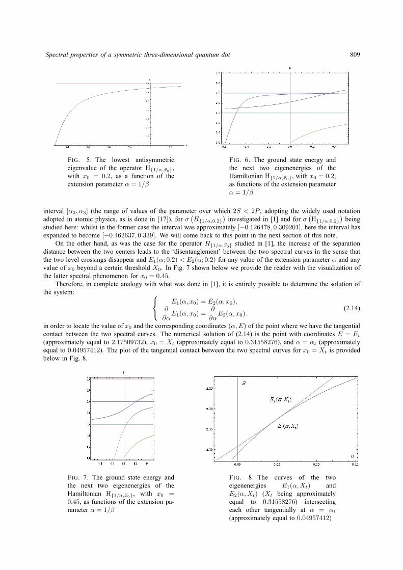
Spectral properties of a symmetric three-dimensional quantum dot 809
FIG. 5. The lowest antisymmetriceigenvalue of the operator H1/α,~x0,with x0 = 0.2, as a function of theextension parameter α = 1/β
FIG. 6. The ground state energy andthe next two eigenenergies of theHamiltonian H1/α,~x0, with x0 = 0.2,as functions of the extension parameterα = 1/β
interval [α2, α3] (the range of values of the parameter over which 2S < 2P , adopting the widely used notationadopted in atomic physics, as is done in [17]), for σ
(H1/α,0.2
)investigated in [1] and for σ
(H1/α,0.2
)being
studied here: whilst in the former case the interval was approximately [−0.126478, 0.309201], here the interval hasexpanded to become [−0.462637, 0.339]. We will come back to this point in the next section of this note.
On the other hand, as was the case for the operator H1/α,~x0 studied in [1], the increase of the separationdistance between the two centers leads to the ‘disentanglement’ between the two spectral curves in the sense thatthe two level crossings disappear and E1(α; 0.2) < E2(α; 0.2) for any value of the extension parameter α and anyvalue of x0 beyond a certain threshold X0. In Fig. 7 shown below we provide the reader with the visualization ofthe latter spectral phenomenon for x0 = 0.45.
Therefore, in complete analogy with what was done in [1], it is entirely possible to determine the solution ofthe system: E1(α, x0) = E2(α, x0),
∂
∂αE1(α, x0) =
∂
∂αE2(α, x0).
(2.14)
in order to locate the value of x0 and the corresponding coordinates (α,E) of the point where we have the tangentialcontact between the two spectral curves. The numerical solution of (2.14) is the point with coordinates E = Et(approximately equal to 2.17509732), x0 = Xt (approximately equal to 0.31558276), and α = αt (approximatelyequal to 0.04957412). The plot of the tangential contact between the two spectral curves for x0 = Xt is providedbelow in Fig. 8.
FIG. 7. The ground state energy andthe next two eigenenergies of theHamiltonian H1/α,~x0, with x0 =0.45, as functions of the extension pa-rameter α = 1/β
FIG. 8. The curves of the twoeigenenergies E1(α,Xt) andE2(α,Xt) (Xt being approximatelyequal to 0.31558276) intersectingeach other tangentially at α = αt(approximately equal to 0.04957412)
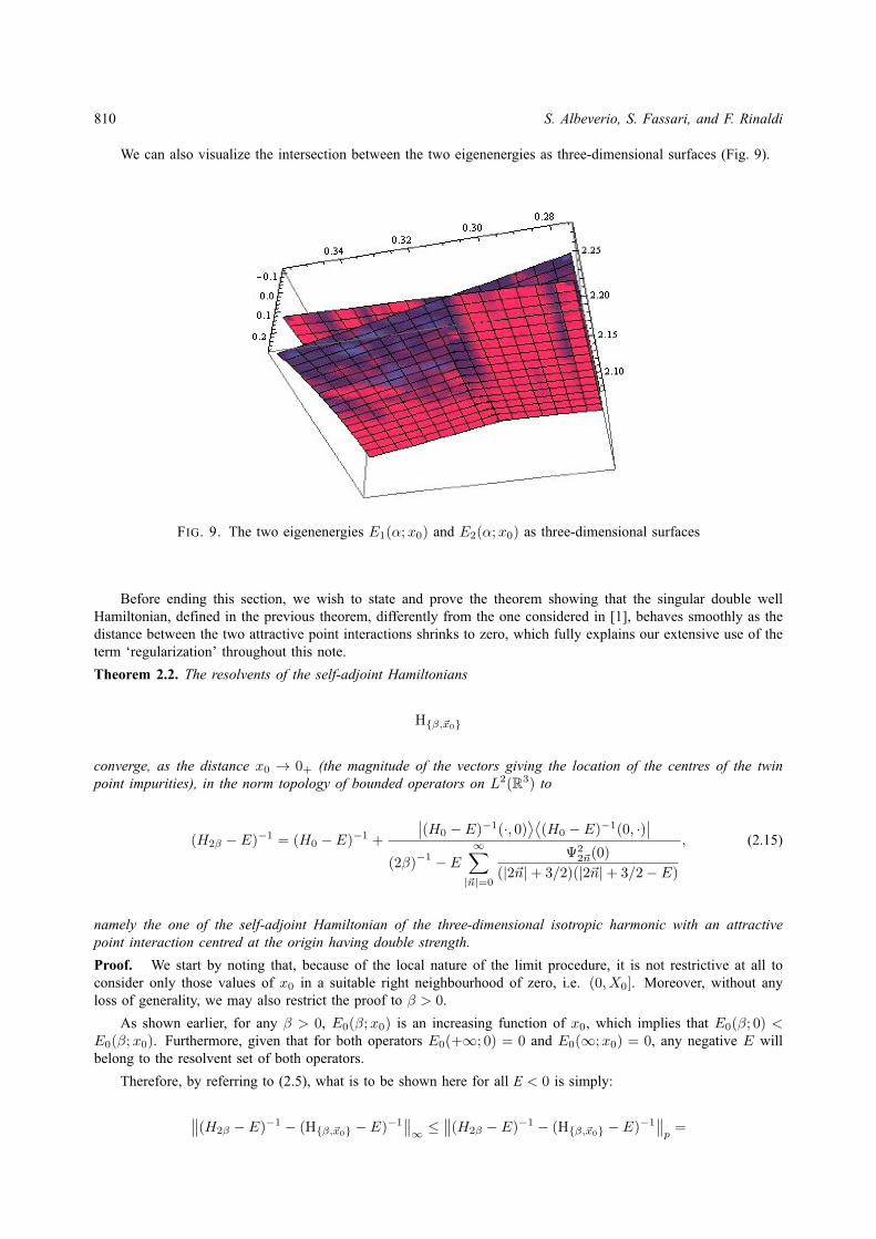
810 S. Albeverio, S. Fassari, and F. Rinaldi
We can also visualize the intersection between the two eigenenergies as three-dimensional surfaces (Fig. 9).
FIG. 9. The two eigenenergies E1(α;x0) and E2(α;x0) as three-dimensional surfaces
Before ending this section, we wish to state and prove the theorem showing that the singular double wellHamiltonian, defined in the previous theorem, differently from the one considered in [1], behaves smoothly as thedistance between the two attractive point interactions shrinks to zero, which fully explains our extensive use of theterm ‘regularization’ throughout this note.
Theorem 2.2. The resolvents of the self-adjoint Hamiltonians
Hβ,~x0
converge, as the distance x0 → 0+ (the magnitude of the vectors giving the location of the centres of the twinpoint impurities), in the norm topology of bounded operators on L2(R3) to
(H2β − E)−1 = (H0 − E)−1 +
∣∣(H0 − E)−1(·, 0)⟩⟨
(H0 − E)−1(0, ·)∣∣
(2β)−1 − E
∞∑|~n|=0
Ψ22~n(0)
(|2~n|+ 3/2)(|2~n|+ 3/2− E)
, (2.15)
namely the one of the self-adjoint Hamiltonian of the three-dimensional isotropic harmonic with an attractivepoint interaction centred at the origin having double strength.
Proof. We start by noting that, because of the local nature of the limit procedure, it is not restrictive at all toconsider only those values of x0 in a suitable right neighbourhood of zero, i.e. (0, X0]. Moreover, without anyloss of generality, we may also restrict the proof to β > 0.
As shown earlier, for any β > 0, E0(β;x0) is an increasing function of x0, which implies that E0(β; 0) <E0(β;x0). Furthermore, given that for both operators E0(+∞; 0) = 0 and E0(∞;x0) = 0, any negative E willbelong to the resolvent set of both operators.
Therefore, by referring to (2.5), what is to be shown here for all E < 0 is simply:
∥∥(H2β − E)−1 − (Hβ,~x0 − E)−1∥∥∞ ≤
∥∥(H2β − E)−1 − (Hβ,~x0 − E)−1∥∥p
=
Spectral properties of a symmetric three-dimensional quantum dot 811∥∥∥∥∥∥∥∥∥∥∥
∣∣(H0 − E)−1(·, 0)
⟩⟨(H0 − E)−1(0, ·)
∣∣(2β)
−1 − E∞∑|~n|=0
Ψ22~n(0)
(|2~n|+ 3/2)(|2~n|+ 3/2− E)
−∣∣(H0 − E)−1s (·, ~x0)
⟩⟨(H0 − E)−1s (~x0, ·)
∣∣(2β)
−1 − E∞∑|~n|=0
Ψ22~n(~x0)
(|2~n|+ 3/2)(|2~n|+ 3/2− E)
⊕∣∣(H0 − E)−1as (·, ~x0)
⟩⟨(H0 − E)−1as (~x0, ·)
∣∣(2β)
−1+ lim`→+∞
∑|~n|=0
Ψ22~n(~x0)
|2~n|+ 3/2−∑|~n|=0
ψ(x0)22n1+1ψ22n2
(0)ψ22n3
(0)
2n1 + 2n2 + 2n3 + 5/2− E
∥∥∥∥∥∥∥∥∥∥∥∥p
→ 0, (2.16)
as x0 → 0+, for any Schatten norm of index p > 3 (the fact that the resolvent of H0 belongs to any Schatten idealwith index p > 3 is shown in [9]). Since both direct summands inside the norm are operators of finite rank, theleft hand side of (2.16) is bounded from above by:∥∥∥∥∥∥∥∥∥∥∥
∣∣(H0 − E)−1(·, 0)⟩⟨
(H0 − E)−1(0, ·)∣∣
(2β)−1 − E
∞∑|~n|=0
Ψ22~n(0)
(|2~n|+ 3/2)(|2~n|+ 3/2− E)
−∣∣(H0 − E)−1s (·, ~x0)
⟩⟨(H0 − E)−1s (~x0, ·)
∣∣(2β)
−1 − E∞∑|~n|=0
Ψ22~n(~x0)
(|2~n|+ 3/2)(|2~n|+ 3/2− E)
∥∥∥∥∥∥∥∥∥∥∥1
+
∥∥∥∥∥∥∥∥∥∥∥∥∣∣(H0 − E)−1as (·, ~x0)
⟩⟨(H0 − E)−1as (~x0, ·)
∣∣(2β)
−1+ lim`→+∞
∑|~n|=0
Ψ22~n(~x0)
|2~n|+ 3/2−∑|~n|=0
ψ(x0)22n1+1ψ22n2
(0)ψ22n3
(0)
2n1 + 2n2 + 2n3 + 5/2− E
∥∥∥∥∥∥∥∥∥∥∥∥1
. (2.17)
Let us deal with the limit of the first summand. Of course, if we can prove that the second term inside thenorm converges to the first one in T1(L2(R3)) (the norm on the trace class operators acting on L2(R3)), then thenorm of their difference will necessarily converge to zero.
As can be guessed, the proof is bound to be rather similar to the one of Theorem 2.2(b) in [10] for theone-dimensional analog of the model since the behavior of the following series will play a crucial role:
((H0)−1s (~x0, ·), (H0 − E)−1s (·, ~x0)
)=
∞∑|~n|=0
Ψ22~n(~x0)
(|2~n|+ 3/2)(|2~n|+ 3/2− E), (2.18)
∥∥(H0 − E)−1s (~x0, ·)∥∥22
=
∞∑|~n|=0
Ψ22~n(~x0)
(|2~n|+ 3/2− E)2= (H0 − E)−2s (~x0, ~x0). (2.19)
As a consequence of the estimate (3.8) in [1], it is evident that, in order to take advantage of the dominatedconvergence theorem, it will not be possible to use the square of the uniform norm ‖ψ2n‖2∞, as was done in theone-dimensional case, since the latter decays only like 1/(2n)1/6 (see [21, 22]), a decay not sufficiently rapid toensure the convergence of
∞∑n=0
‖ψ2n‖2∞(2n+ 1/2)2/3
.
However, given that the limit procedure involves only those x0’s in (0, X0] for some suitable X0 > 0, weneed not use the global maximum of ψ2n in our quest for a dominating `1-sequence but rather the one over such aright vicinity of zero. Then, we can take advantage of the estimates (21) in [23] in order to state that, by choosingany X0 ≤
√3− 1, we are guaranteed that there exists a constant C such that:
∞∑n=0
ψ22n(x0)
(2n+ 1/2)2/3≤ 22/3√
π+
∞∑n=1
C2
(2n)1/2(2n+ 1/2)2/3<∞, (2.20)
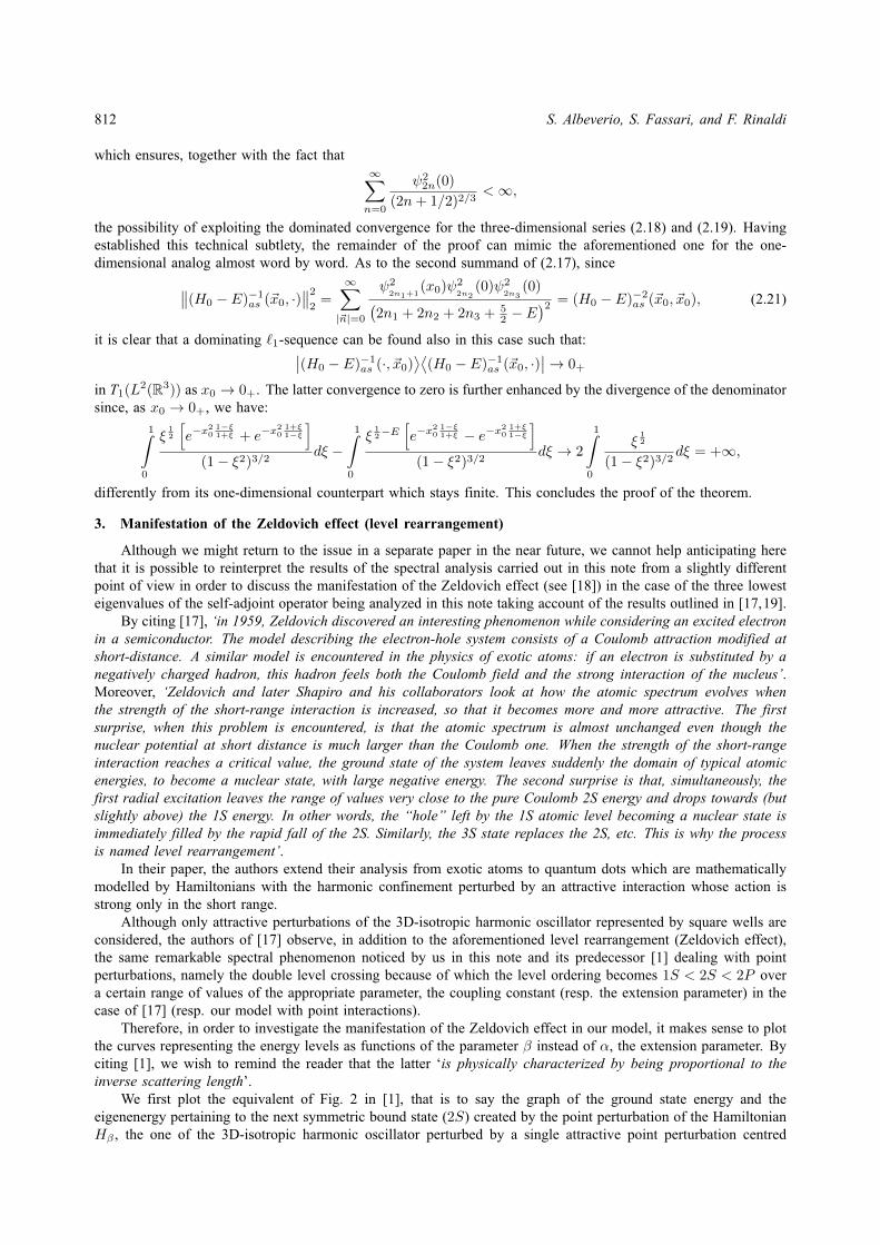
812 S. Albeverio, S. Fassari, and F. Rinaldi
which ensures, together with the fact that∞∑n=0
ψ22n(0)
(2n+ 1/2)2/3<∞,
the possibility of exploiting the dominated convergence for the three-dimensional series (2.18) and (2.19). Havingestablished this technical subtlety, the remainder of the proof can mimic the aforementioned one for the one-dimensional analog almost word by word. As to the second summand of (2.17), since∥∥(H0 − E)−1as (~x0, ·)
∥∥22
=
∞∑|~n|=0
ψ22n1+1
(x0)ψ22n2
(0)ψ22n3
(0)(2n1 + 2n2 + 2n3 + 5
2 − E)2 = (H0 − E)−2as (~x0, ~x0), (2.21)
it is clear that a dominating `1-sequence can be found also in this case such that:∣∣(H0 − E)−1as (·, ~x0)⟩⟨
(H0 − E)−1as (~x0, ·)∣∣→ 0+
in T1(L2(R3)) as x0 → 0+. The latter convergence to zero is further enhanced by the divergence of the denominatorsince, as x0 → 0+, we have:
1∫0
ξ12
[e−x
20
1−ξ1+ξ + e−x
20
1+ξ1−ξ
](1− ξ2)3/2
dξ −1∫
0
ξ12−E
[e−x
20
1−ξ1+ξ − e−x
20
1+ξ1−ξ
](1− ξ2)3/2
dξ → 2
1∫0
ξ12
(1− ξ2)3/2dξ = +∞,
differently from its one-dimensional counterpart which stays finite. This concludes the proof of the theorem.
3. Manifestation of the Zeldovich effect (level rearrangement)
Although we might return to the issue in a separate paper in the near future, we cannot help anticipating herethat it is possible to reinterpret the results of the spectral analysis carried out in this note from a slightly differentpoint of view in order to discuss the manifestation of the Zeldovich effect (see [18]) in the case of the three lowesteigenvalues of the self-adjoint operator being analyzed in this note taking account of the results outlined in [17,19].
By citing [17], ‘in 1959, Zeldovich discovered an interesting phenomenon while considering an excited electronin a semiconductor. The model describing the electron-hole system consists of a Coulomb attraction modified atshort-distance. A similar model is encountered in the physics of exotic atoms: if an electron is substituted by anegatively charged hadron, this hadron feels both the Coulomb field and the strong interaction of the nucleus’.Moreover, ‘Zeldovich and later Shapiro and his collaborators look at how the atomic spectrum evolves whenthe strength of the short-range interaction is increased, so that it becomes more and more attractive. The firstsurprise, when this problem is encountered, is that the atomic spectrum is almost unchanged even though thenuclear potential at short distance is much larger than the Coulomb one. When the strength of the short-rangeinteraction reaches a critical value, the ground state of the system leaves suddenly the domain of typical atomicenergies, to become a nuclear state, with large negative energy. The second surprise is that, simultaneously, thefirst radial excitation leaves the range of values very close to the pure Coulomb 2S energy and drops towards (butslightly above) the 1S energy. In other words, the “hole” left by the 1S atomic level becoming a nuclear state isimmediately filled by the rapid fall of the 2S. Similarly, the 3S state replaces the 2S, etc. This is why the processis named level rearrangement’.
In their paper, the authors extend their analysis from exotic atoms to quantum dots which are mathematicallymodelled by Hamiltonians with the harmonic confinement perturbed by an attractive interaction whose action isstrong only in the short range.
Although only attractive perturbations of the 3D-isotropic harmonic oscillator represented by square wells areconsidered, the authors of [17] observe, in addition to the aforementioned level rearrangement (Zeldovich effect),the same remarkable spectral phenomenon noticed by us in this note and its predecessor [1] dealing with pointperturbations, namely the double level crossing because of which the level ordering becomes 1S < 2S < 2P overa certain range of values of the appropriate parameter, the coupling constant (resp. the extension parameter) in thecase of [17] (resp. our model with point interactions).
Therefore, in order to investigate the manifestation of the Zeldovich effect in our model, it makes sense to plotthe curves representing the energy levels as functions of the parameter β instead of α, the extension parameter. Byciting [1], we wish to remind the reader that the latter ‘is physically characterized by being proportional to theinverse scattering length’.
We first plot the equivalent of Fig. 2 in [1], that is to say the graph of the ground state energy and theeigenenergy pertaining to the next symmetric bound state (2S) created by the point perturbation of the HamiltonianHβ , the one of the 3D-isotropic harmonic oscillator perturbed by a single attractive point perturbation centred
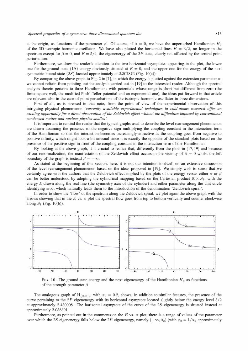
Spectral properties of a symmetric three-dimensional quantum dot 813
at the origin, as functions of the parameter β. Of course, if β = 0, we have the unperturbed Hamiltonian H0
of the 3D-isotropic harmonic oscillator. We have also plotted the horizontal lines E = 3/2, no longer in thespectrum except for β = 0, and E = 5/2, the eigenenergy of the 2P state, clearly not affected by the central pointperturbation.
Furthermore, we draw the reader’s attention to the two horizontal asymptotes appearing in the plot, the lowerone for the ground state (1S) energy obviously situated at E = 0, and the upper one for the energy of the nextsymmetric bound state (2S) located approximately at 2.307876 (Fig. 10(a)).
By comparing the above graph to Fig. 2 in [1], in which the energy is plotted against the extension parameter α,we cannot refrain from pointing out the analysis carried out in [19] to the interested reader. Although the spectralanalysis therein pertains to three Hamiltonians with potentials whose range is short but different from zero (thefinite square well, the modified Poshl-Teller potential and an exponential one), the ideas put forward in that articleare relevant also in the case of point perturbations of the isotropic harmonic oscillator in three dimensions.
First of all, as is stressed in that note, from the point of view of the experimental observation of thisintriguing physical phenomenon ‘currently available experimental techniques in cold-atoms research offer anexciting opportunity for a direct observation of the Zeldovich effect without the difficulties imposed by conventionalcondensed matter and nuclear physics studies’.
It is important to remind the reader that the typical graphs used to describe the level rearrangement phenomenonare drawn assuming the presence of the negative sign multiplying the coupling constant in the interaction termof the Hamiltonian so that the interaction becomes increasingly attractive as the coupling goes from negative topositive infinity, which might look a bit unusual since it is exactly the opposite of the standard plots based on thepresence of the positive sign in front of the coupling constant in the interaction term of the Hamiltonian.
By looking at the above graph, it is crucial to realize that, differently from the plots in [17, 19] and becauseof our renormalization, the manifestation of the Zeldovich effect occurs in the vicinity of β = 0 whilst the leftboundary of the graph is instead β = −∞.
As stated at the beginning of this section, here, it is not our intention to dwell on an extensive discussionof the level rearrangement phenomenon based on the ideas proposed in [19]. We simply wish to stress that wecertainly agree with the authors that the Zeldovich effect implied by the plots of the energy versus either α or βcan be better understood by adopting the cylindrical mapping based on the Cartesian product R × S1, with theenergy E drawn along the real line (the symmetry axis of the cylinder) and either parameter along the unit circleidentifying ±∞, which naturally leads them to the introduction of the denomination ‘Zeldovich spiral’.
In order to show the ‘flow’ of the spectrum along the Zeldovich spiral, we plot again the above graph with thearrows showing that in the E vs. β plot the spectral flow goes from top to bottom vertically and counter clockwisealong S1 (Fig. 10(b)).
FIG. 10. The ground state energy and the next eigenenergy of the Hamiltonian Hβ as functionsof the strength parameter β
The analogous graph of Hβ,~x0, with x0 = 0.2, shows, in addition to similar features, the presence of thecurve pertaining to the 2P eigenenergy with its horizontal asymptote located slightly below the energy level 5/2at approximately 2.450008. The horizontal asymptote of the curve of the 2S eigenenergy is situated instead atapproximately 2.058391.
Furthermore, as pointed out in the comments on the E vs. α plot, there is a range of values of the parameterover which the 2S eigenenergy falls below the 2P eigenenergy, namely (−∞, β2) (with β2 = 1/α2 approximately
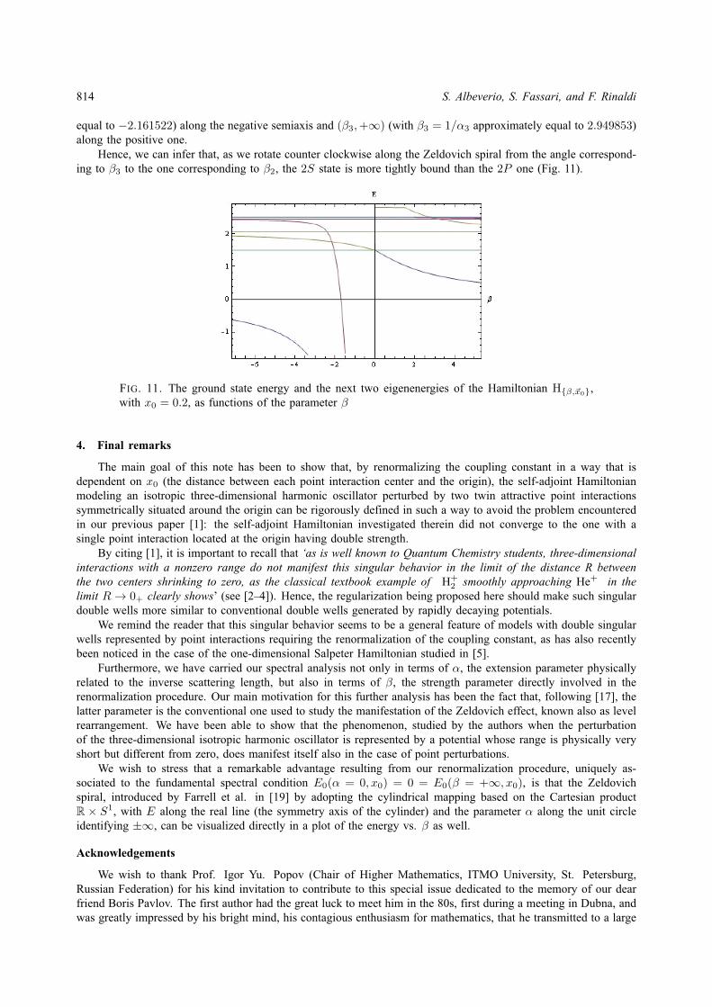
814 S. Albeverio, S. Fassari, and F. Rinaldi
equal to −2.161522) along the negative semiaxis and (β3,+∞) (with β3 = 1/α3 approximately equal to 2.949853)along the positive one.
Hence, we can infer that, as we rotate counter clockwise along the Zeldovich spiral from the angle correspond-ing to β3 to the one corresponding to β2, the 2S state is more tightly bound than the 2P one (Fig. 11).
FIG. 11. The ground state energy and the next two eigenenergies of the Hamiltonian Hβ,~x0,with x0 = 0.2, as functions of the parameter β
4. Final remarks
The main goal of this note has been to show that, by renormalizing the coupling constant in a way that isdependent on x0 (the distance between each point interaction center and the origin), the self-adjoint Hamiltonianmodeling an isotropic three-dimensional harmonic oscillator perturbed by two twin attractive point interactionssymmetrically situated around the origin can be rigorously defined in such a way to avoid the problem encounteredin our previous paper [1]: the self-adjoint Hamiltonian investigated therein did not converge to the one with asingle point interaction located at the origin having double strength.
By citing [1], it is important to recall that ‘as is well known to Quantum Chemistry students, three-dimensionalinteractions with a nonzero range do not manifest this singular behavior in the limit of the distance R betweenthe two centers shrinking to zero, as the classical textbook example of H+
2 smoothly approaching He+ in thelimit R→ 0+ clearly shows’ (see [2–4]). Hence, the regularization being proposed here should make such singulardouble wells more similar to conventional double wells generated by rapidly decaying potentials.
We remind the reader that this singular behavior seems to be a general feature of models with double singularwells represented by point interactions requiring the renormalization of the coupling constant, as has also recentlybeen noticed in the case of the one-dimensional Salpeter Hamiltonian studied in [5].
Furthermore, we have carried our spectral analysis not only in terms of α, the extension parameter physicallyrelated to the inverse scattering length, but also in terms of β, the strength parameter directly involved in therenormalization procedure. Our main motivation for this further analysis has been the fact that, following [17], thelatter parameter is the conventional one used to study the manifestation of the Zeldovich effect, known also as levelrearrangement. We have been able to show that the phenomenon, studied by the authors when the perturbationof the three-dimensional isotropic harmonic oscillator is represented by a potential whose range is physically veryshort but different from zero, does manifest itself also in the case of point perturbations.
We wish to stress that a remarkable advantage resulting from our renormalization procedure, uniquely as-sociated to the fundamental spectral condition E0(α = 0, x0) = 0 = E0(β = +∞, x0), is that the Zeldovichspiral, introduced by Farrell et al. in [19] by adopting the cylindrical mapping based on the Cartesian productR × S1, with E along the real line (the symmetry axis of the cylinder) and the parameter α along the unit circleidentifying ±∞, can be visualized directly in a plot of the energy vs. β as well.
Acknowledgements
We wish to thank Prof. Igor Yu. Popov (Chair of Higher Mathematics, ITMO University, St. Petersburg,Russian Federation) for his kind invitation to contribute to this special issue dedicated to the memory of our dearfriend Boris Pavlov. The first author had the great luck to meet him in the 80s, first during a meeting in Dubna, andwas greatly impressed by his bright mind, his contagious enthusiasm for mathematics, that he transmitted to a large
Spectral properties of a symmetric three-dimensional quantum dot 815
number of students. One of the topics we discussed was the subject of point interactions. He gave fundamentalcontributions to this area and, more generally, to spectral theory. The contacts with him and his research associateshappily accompanied our further scientific life.
The second author had the privilege of meeting him in February 1991 as we were both visiting Prof. Albeverioin Bochum. It was a great pleasure, shared also by the third author, to see him twenty-four years later in St.Petersburg on the occasion of the international conference ‘Mathematical Challenge of Quantum Transport inNanosystems’, held at ITMO University, St. Petersburg, Russian Federation (9–11 September 2015). It is withgreat gratitude that we acknowledge his scientific legacy and dedicate this work to his memory.
References
[1] Albeverio S., Fassari S., Rinaldi F. Spectral properties of a symmetric three-dimensional quantum dot with a pair of identical attractiveδ-impurities symmetrically situated around the origin. Nanosystems: Physics, Chemistry, Mathematics, 2016, 7 (2), P. 268–289.
[2] Schmidtke H.-H. Quantenchemie. Weinheim: VCH, 1987 (in German).[3] Byers Brown W., Steiner E. On the electronic energy of a one-electron diatomic molecule near the united atom. Journal of Chemical
Physics, 1966, 44, P. 3934.[4] Klaus M. On H+
2 for small internuclear separation. Journal of Physics A: Mathematical and General, 1983, 16, P. 2709–2720.[5] Albeverio S., Fassari S., Rinaldi F. The discrete spectrum of the spinless Salpeter Hamiltonian perturbed by δ-interactions. Journal of
Physics A: Mathematical and Theoretical, 2015, 48 (18), P. 185301.[6] Albeverio S., Gesztesy F., Høegh-Krohn R., Holden H. Solvable models in Quantum Mechanics. AMS (Chelsea Series) second edition,
2004.[7] Albeverio S., Kurasov P. Singular Perturbations of Differential Operators: Solvable Type Operators. Cambridge University Press, 2000.[8] Albeverio S., Fassari S., Rinaldi F. A remarkable spectral feature of the Schrodinger Hamiltonian of the harmonic oscillator perturbed
by an attractive δ′-interaction centred at the origin: double degeneracy and level crossing. Journal of Physics A: Mathematical andTheoretical, 2013, 46 (38), P. 385305.
[9] Fassari S., Inglese G. Spectroscopy of a three-dimensional isotropic harmonic oscillator with a δ-type perturbation. Helvetica PhysicaActa, 1996, 69, P. 130–140.
[10] Fassari S., Rinaldi F. On the spectrum of the Schrodinger Hamiltonian of the one-dimensional harmonic oscillator perturbed by twoidentical attractive point interactions. Reports on Mathematical Physics, 2012, 69 (3), P. 353–370.
[11] Reed M., Simon B. Fourier Analysis, Self-adjointness – Methods of Modern Mathematical Physics II, Academic Press NY, 1975.[12] Exner P., Neidhardt H., Zagrebnov V.A. Potential approximations to δ’: an inverse Klauder phenomenon with norm resolvent convergence.
Communications in Mathematical Physics, 2001, 22, P. 4593–4612.[13] Fassari S., Rinaldi F. On the spectrum of the Schrodinger Hamiltonian with a particular configuration of three point interactions. Reports
on Mathematical Physics, 2009, 64 (3), P. 367–393.[14] Albeverio S., Fassari S., Rinaldi F. The Hamiltonian of the harmonic oscillator with an attractive δ’-interaction centred at the origin as
approximated by the one with a triple of attractive δ-interactions. Journal of Physics A: Mathematical and Theoretical, 2016, 49 (2),P. 025302.
[15] Fassari S., Inglese G. On the spectrum of the harmonic oscillator with a δ-type perturbation. Helvetica Physica Acta, 1994, 67, P. 650–659.[16] Fassari S., Inglese G. On the spectrum of the harmonic oscillator with a δ-type perturbation II. Helvetica Physica Acta, 1997, 70,
P. 858–865.[17] Combescure M., Khare A., et al. Level rearrangement in exotic atoms and quantum dots. International Journal of Modern Physics B,
2006, 21 (22), P. 3765.[18] Zeldovich Ya.B. Energy levels in a distorted Coulomb field. Soviet Journal Solid State, 1960, 1, P. 1497.[19] Farrell A., MacDonald Z., van Zyl B. The Zeldovich effect in harmonically trapped, ultra-cold quantum gases. Journal of Physics A:
Mathematical and Theoretical, 2012, 45, P. 045303.[20] Bruning J., Geyler V., Lobanov I. Spectral properties of a short-range impurity in a quantum dot. Journal of Mathematical Physics, 2004,
45, P. 1267–1290.[21] Plancherel M., Rotach W. Sur les valeurs asymptotiques des polynomes d’Hermite. Commentarii Mathematici Helvetici, 1929, 1 (1),
P. 227–254.[22] Reed M., Simon B. Functional Analysis – Methods of Modern Mathematical Physics I. Academic Press, NY, 1972.[23] Mityagin B., Siegl P. Root system of singular perturbations of the harmonic oscillator type operators. Letters in Mathematical Physics,
2016, 106 (2), P. 147–167.
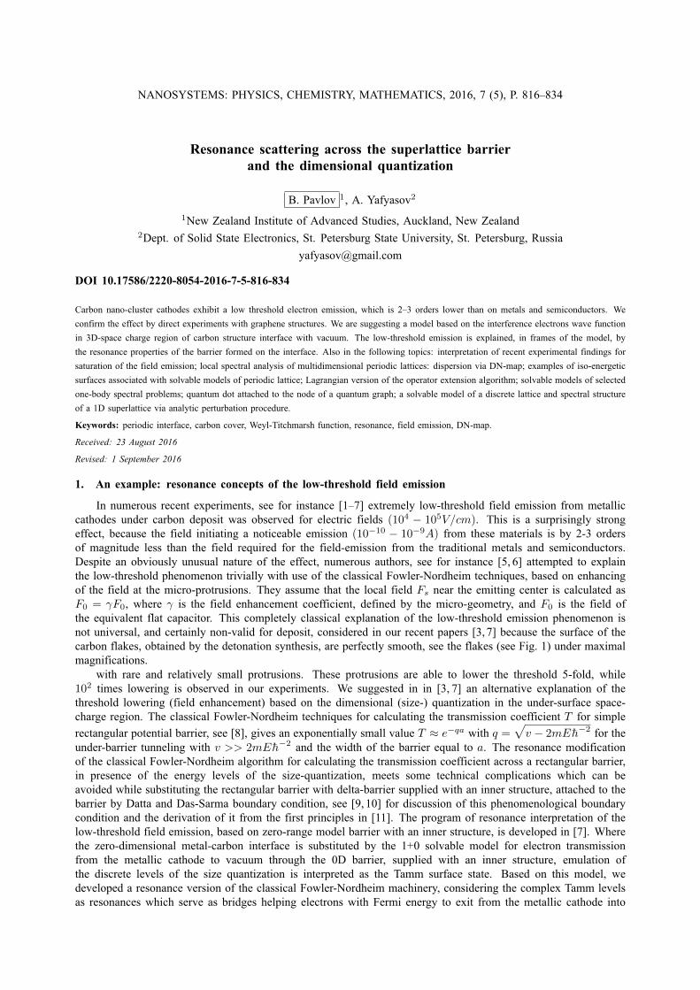
NANOSYSTEMS: PHYSICS, CHEMISTRY, MATHEMATICS, 2016, 7 (5), P. 816–834
Resonance scattering across the superlattice barrierand the dimensional quantization
B. Pavlov 1, A. Yafyasov2
1New Zealand Institute of Advanced Studies, Auckland, New Zealand2Dept. of Solid State Electronics, St. Petersburg State University, St. Petersburg, Russia
DOI 10.17586/2220-8054-2016-7-5-816-834
Carbon nano-cluster cathodes exhibit a low threshold electron emission, which is 2–3 orders lower than on metals and semiconductors. We
confirm the effect by direct experiments with graphene structures. We are suggesting a model based on the interference electrons wave function
in 3D-space charge region of carbon structure interface with vacuum. The low-threshold emission is explained, in frames of the model, by
the resonance properties of the barrier formed on the interface. Also in the following topics: interpretation of recent experimental findings for
saturation of the field emission; local spectral analysis of multidimensional periodic lattices: dispersion via DN-map; examples of iso-energetic
surfaces associated with solvable models of periodic lattice; Lagrangian version of the operator extension algorithm; solvable models of selected
one-body spectral problems; quantum dot attached to the node of a quantum graph; a solvable model of a discrete lattice and spectral structure
of a 1D superlattice via analytic perturbation procedure.
Keywords: periodic interface, carbon cover, Weyl-Titchmarsh function, resonance, field emission, DN-map.
Received: 23 August 2016
Revised: 1 September 2016
1. An example: resonance concepts of the low-threshold field emission
In numerous recent experiments, see for instance [1–7] extremely low-threshold field emission from metalliccathodes under carbon deposit was observed for electric fields (104 − 105V/cm). This is a surprisingly strongeffect, because the field initiating a noticeable emission (10−10 − 10−9A) from these materials is by 2-3 ordersof magnitude less than the field required for the field-emission from the traditional metals and semiconductors.Despite an obviously unusual nature of the effect, numerous authors, see for instance [5, 6] attempted to explainthe low-threshold phenomenon trivially with use of the classical Fowler-Nordheim techniques, based on enhancingof the field at the micro-protrusions. They assume that the local field Fs near the emitting center is calculated asF0 = γF0, where γ is the field enhancement coefficient, defined by the micro-geometry, and F0 is the field ofthe equivalent flat capacitor. This completely classical explanation of the low-threshold emission phenomenon isnot universal, and certainly non-valid for deposit, considered in our recent papers [3, 7] because the surface of thecarbon flakes, obtained by the detonation synthesis, are perfectly smooth, see the flakes (see Fig. 1) under maximalmagnifications.
with rare and relatively small protrusions. These protrusions are able to lower the threshold 5-fold, while102 times lowering is observed in our experiments. We suggested in in [3, 7] an alternative explanation of thethreshold lowering (field enhancement) based on the dimensional (size-) quantization in the under-surface space-charge region. The classical Fowler-Nordheim techniques for calculating the transmission coefficient T for simple
rectangular potential barrier, see [8], gives an exponentially small value T ≈ e−qa with q =√v − 2mEh−2 for the
under-barrier tunneling with v >> 2mEh−2 and the width of the barrier equal to a. The resonance modificationof the classical Fowler-Nordheim algorithm for calculating the transmission coefficient across a rectangular barrier,in presence of the energy levels of the size-quantization, meets some technical complications which can beavoided while substituting the rectangular barrier with delta-barrier supplied with an inner structure, attached to thebarrier by Datta and Das-Sarma boundary condition, see [9, 10] for discussion of this phenomenological boundarycondition and the derivation of it from the first principles in [11]. The program of resonance interpretation of thelow-threshold field emission, based on zero-range model barrier with an inner structure, is developed in [7]. Wherethe zero-dimensional metal-carbon interface is substituted by the 1+0 solvable model for electron transmissionfrom the metallic cathode to vacuum through the 0D barrier, supplied with an inner structure, emulation ofthe discrete levels of the size quantization is interpreted as the Tamm surface state. Based on this model, wedeveloped a resonance version of the classical Fowler-Nordheim machinery, considering the complex Tamm levelsas resonances which serve as bridges helping electrons with Fermi energy to exit from the metallic cathode into
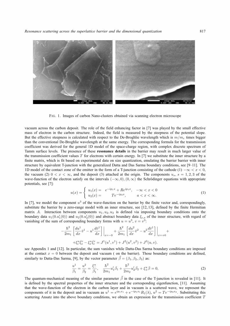
Resonance scattering across the superlattice barrier and the dimensional quantization 817
FIG. 1. Images of carbon Nano-clusters obtained via scanning electron microscope
vacuum across the carbon deposit. The role of the field enhancing factor in [7] was played by the small effectivemass of electron in the carbon structure. Indeed, the field is measured by the steepness of the potential slope.But the effective steepness is calculated with respect to the De-Broghlie wavelength which is m/me times biggerthan the conventional De-Broghlie wavelength at the same energy. The corresponding formula for the transmissioncoefficient was derived for the general 1D model of the space-charge region, with complex discrete spectrum ofTamm surface levels. The presence of these resonance details in the barrier may result in much larger value ofthe transmission coefficient values T for electrons with certain energy. In [7] we substitute the inner structure by afinite matrix, which is fit based on experimental data on size quantization, emulating the barrier barrier with innerstructure by equivalent T-junction with the generalized Datta and Das Sarma boundary conditions, see [9–11]. The1D model of the contact zone of the emitter in the form of a T-junction consisting of the cathode (1) −∞ < x < 0,the vacuum (2) 0 < x < ∞, and the deposit (3) attached at the origin. The components us, s = 1, 2, 3 of thewave-function of the electron satisfy on the intervals (−∞, 0), (0,∞) the Schrodinger equations with appropriatepotentials, see [7]:
u(x) =
u1(x) = e−ip1x +Reip1x, −∞ < x < 0
u2(x) = Te−ip2x, a < x <∞.(1)
In [7], we model the component u3 of the wave-function on the barrier by the finite vector and, correspondingly,substitute the barrier by a zero-range model with an inner structure, see [12, 13], defined by the finite Hermitianmatrix A. Interaction between components u1, u2, u3 is defined via imposing boundary conditions onto theboundary data u1(0.u′1(0)) and u2(0.u′2(0)) and abstract boundary data ξc,s of the inner structure, with regard ofvanishing of the sum of corresponding boundary forms with u = u3, v = v3:
− h2
2m1
[du1
dxv1 − u1 dv
1
dx
] ∣∣∣∣x=−0
+h2
2m1
[du2
dxv2 − u2 dv
1
dx
] ∣∣∣∣x=+0
+
+ξuc ξvs − ξus ξvc = J1(u1, v1) + J2(u2, v2) + J3(u, v).
see Appendix 1 and [12]. In particular, the sum vanishes while Datta-Das Sarma boundary conditions are imposedat the contact x = 0 between the deposit and vacuum ( on the barrier). Those boundary conditions are defined,similarly to Datta-Das Sarma, [9], by the vector parameter ~β = (β1, β2, β3) as:
u1
β1=u2
β2=ξu−β1,
h2
2m1u′1β1 +
h2
2m2u′2β2 + ξu+β = 0, (2)
The quantum-mechanical meaning of the similar parameter ~β in the case of the T-junction is revealed in [11]. Itis defined by the spectral properties of the inner structure and the corresponding eigenfunction, [11]. Assumingthat the wave-function of the electron in the carbon layer and in vacuum is a scattered wave, we represent thecomponents of it in the deposit and in vacuum as u1 = eip1x1 + e−ip1x1R1(λ), u2 = Te−ip2x2 . Substituting thisscattering Ansatz into the above boundary conditions, we obtain an expression for the transmission coefficient T
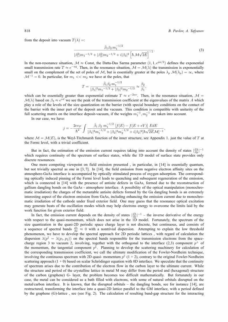
818 B. Pavlov, A. Yafyasov
from the deposit into vacuum T (λ) =:
β1β2m−1/21
|β21 |m1
−1/2 + |β22 |m2
−1/2 + i|β3|2[hM√
2E]−1 . (3)
In the non-resonance situation, M ≈ Const, the Datta-Das Sarma parameter (1, 1, eqa/2) defines the exponentialsmall transmission rate T ≈ e−aq . Then, in the resonance situation, M =M(λ) the transmission is exponentiallysmall on the complement of the set of poles of M, but is essentially greater at the poles λp M(λp) = ∞, whereM−1 = 0. In particular, for m1 << m2 we have at the poles, that
T =β1β2m
−1/21
|β1|2m1−1/2 + |β2|2m2
−1/2≈ β2
β1,
which can be essentially greater than exponential estimate T ≈ e−2av . Then, in the resonance situation, M =M(λ) based on β3 ≈ evd we see the peak of the transmission coefficient at the eigenvalues of the matrix A whichplay a role of the levels of the size quantization on the barrier (with special boundary conditions on the contact ofthe barrier with the inner part of the deposit and the vacuum. This condition is compatible with unitarity of thefull scattering matrix on the interface deposit-vacuum, if the weights m−1
1 ,m−12 are taken into account.
In our case, we have:
j = −2evF
h2
∫β1 β2 m
−1/21 [f(E)− f(E + eV )] EdE
|β1|2m−1/21 + |β2|2m−1/2
2 + i|β2|2[h√
2EM]−1,
whereM =M(E), is the Weyl-Titchmarsh function of the inner structure, see Appendix 1. just the value of T atthe Fermi level, with a trivial coefficient.
But in fact, the estimation of the emission current requires taking into account the density of states |∂λ∂p |−1
which requires continuity of the spectrum of surface states, while the 1D model of surface state provides onlydiscrete resonances.
One more competing viewpoint on field emission presented , in particular, in [14] is essentially quantum,but not trivially spectral as one in [3, 7]. In [14], the field emission from negative electron affinity sites on theatmosphere-GaAs interface is accompanied by optically stimulated process of oxygen adsorption. The correspond-ing optically induced pinning of the Fermi level leads to quenching and subsequent regeneration of the emission,which is connected in [14] with the presence of antisite defects in GaAs, formed due to the reconstruction ofgallium dangling bonds on the GaAs - atmosphere interface. A possibility of the optical manipulation (monochro-matic irradiation) the charges of the metastable antisite defects formed by the Ga dangling bonds is an extremelyinteresting aspect of the electron emission from GaAs, including enhancing the emission current due to monochro-matic irradiation of the cathode under fixed exterior field. One may guess that the resonance optical excitationmay generate beats of the oscillation modes which may help electrons energy to overcome the limits laid by thework function for given exterior field.
In fact, the emission current depends on the density of states |dλdp |−1 – the inverse derivative of the energy
with respect to the quasi-momentum, which does not arise in the 1D model. Fortunately, the spectrum of thesize quantization in the quasi-2D periodic space charge layer is not discrete, but continuous, and consists ofa sequence of spectral bands dλ
dp ≈ 0 with a nontrivial dispersion. Attempting to explain the low thresholdphenomenon, we have to develop the spectral approach for 2D periodic lattices , with regard of calculation thedispersion λ(p‖ = λ(p1, p2)) on the spectral bands responsible for the transmission electrons from the space-charge region 3 to vacuum 2, involving, together with the orthogonal to the interface (2,3) component p⊥ ofthe momentum, the tangential component p‖. Planning to develop the scattering machinery for calculation ofthe corresponding transmission coefficient, we call the ultimate modification of the Fowler-Nordheim technique,involving the continuous spectrum with 2D quasi- momentum p‖ (1 + 2), contrary to the original Fowler-Nordheimscattering approach (1 + 0) based on scalar Schrodinger equation with 0D interface. We speculate that the continuityof spectrum arises due to the contribution of the electron flow in the carbon layer to the ultimate current. Whilethe structure and period of the crystalline lattice in metal M may differ from the period and (hexagonal) structureof the carbon (graphene) G- layer, the problem becomes too difficult mathematically. But fortunately in ourcase, the metal can be considered as a bath filled with electrons, with some of natural orbitals disrupted on themetal/carbon interface. It is known, that the disrupted orbitals – the dangling bonds, see for instance [14], arerestructured, transforming the interface into a quasi-2D lattice parallel to the GM interface, with a period definedby the graphene (G)-lattice , see (see Fig. 2). The calculation of resulting band-gap structure for the interacting
Resonance scattering across the superlattice barrier and the dimensional quantization 819
FIG. 2. Due to exterior electric field, the space-charge layer (SC) on the interface of the carbonand metal is restructured into periodic quasi-2D lattice with a rectangular period, as shown. Thehorizontal periodicity of the structure is not affected by the exterior electric field, normal to theinterface, but the total band-gap structure is perturbed due to interaction of two periodic lattices,with equal periods, on the interface: one in metal M, another in carbon, G , resulting in thearisal of flat thin spectral bands of the size quantization
quasi-2D M and G lattices requires special analytical techniques using the Dirichlet-to-Neumann map, which ispresented in section 3 below.
2. Interpretation of recent experimental findings for saturation of the field emission
Contrary to the basic (2 + 1) model of the cathode, see Fig. 2. DN formalism, see below, section 4, allowsus to calculate the dispersion function of the spectral band of the size quantization in terms of the structure of thespace-charge region and the electric field applied.
But in fact the estimation of the emission current requires taking into account the density of states |∂λ∂p |−1,
which can’t be introduced properly in the 1D model. Fortunately, the spectrum of the size quantization in the quasi2D periodic space charge layer is continuous, and consists of a sequence of flat spectral bands, with nontrivialdispersion λ = λ(p). The ultimate version of explanation of the low threshold phenomenon, we suggest in thispaper, takes into account both size quantization of electrons in the space-charge layer cv due to perturbation ofthe periodic structure in the space-charge layer in 1D vertical direction p⊥ and the continuity of the correspondingspectrum due to periodicity of the quasi 2D structure in horizontal direction p‖ = (p1, p2). We call the ultimatemodification the “2+1” model of the cathode, see Fig. 1.
DN formalism, see below, section 4, allows calculation of the dispersion function of the spectral band of thesize quantization in terms of the structure of the space-charge period and electric field applied. We are able tocalculate the the gradient of the dispersion function dE = |∇pE(~p)|dp⊥ with E = p2/2m. Then, for the 2-Dsystem, the density of states in the 2-D is calculated as an integral on the surface S of the cathode [15]:
ρ(E) =1
(2πh)2
∫dS
|∇pE|=
1
2πh2
p∂E∂p
=m
2π h2 . (4)
Recent experiments done by our group confirm the continuity of spectrum 2D-size quantization and allow usto estimate the effective mass m∗ and the de Broglie wavelength in space-charge region depending on electron’s
concentration nex =1
q
τ∫0
J(t)dt, where j = I/S, I = 80 A is the current and S ≈ 0.75 cm2 – the area of the
cathode, τ ≈ 2 × 10⁻⁹ s. Monitoring of the current density allows us to estimate the experimental density ofcharges Q = 2.4× 10⁻⁷ Coul/cm2, which corresponds to density of electrons n ≈ 1.3× 1012 cm−2.
On another hand, from the size-quantization theory [15] the 2D density of electrons is estimated as:
n2D =m∗kT
2πh2 ln
(1 + exp
E0 − EFkT
)(5)
Here, m∗ is the effective electron mass, E0—the size-quantization level, EF—the Fermi level. In our case
E0 ≈ EF , nexp = n2D =m∗kT
2πh2 ln 2 (6)
The de Broglie electron wavelength [15] in graphene flakes is:
λ =2πh√
2m∗ (kT ). (7)
820 B. Pavlov, A. Yafyasov
Based on the preceding Equations (6) and (7), we estimate the electron effective mass and the de Broglieelectron
m∗ =(2πh)2
2(kT )(8)
At room temperature, we have λ ≈ 18 nm, m∗ ≤ 10−2 m0.The potential on the space-charge region of the cathode, covered with carbon flakes is defined by the electric
double layers formed by the electric field applied on the metal-carbon and carbon-vacuum interface and orientedby the outer normal looking toward vacuum. The horizontal periodicity of the cover is not affected by the field, butthe vertical periodicity is perturbed by the potential well defined by the electric field, see Fig. 2. We assume thatthe depth of penetration of the field into the carbon layer defines the width of the potential well and the steepnessof its wall. The hexagonal lattice can be represented as a periodic lattice with rectangular periods, 4 carbon atomsin each minimal period.
3. Resonance scattering on a low-dimensional superlattice and field emission from the metal-carboninterface
The above criticism of the resonance 0+1 scenario of the low-threshold field emission may be resolved basedon a combination of Bagraev’s findings in [14] on the periodic reconstruction of dangling bonds and recent resultsof our experimentalists [16], revealing the role of the continuous spectrum of the size quantization. Hereafter,we construct a solvable (2 + 1) model of a periodic 2D lattice on an interface of the Luttinger bath in metaland vacuum and calculate the scattering amplitude depending on resonance properties of the lattice period. Themodel can be used not only for analysis of the low-threshold emission, but also for studying the properties anddynamics stability of electric contact as a detail of a nano-device, or, generally, a quantum network. While simplestzero-range models of 2D lattices in 3D have been thoroughly investigated neglecting the “inner structure” see [17],the use of similar models with inner structure allows to interpret various instabilities of the contacts based onresonance properties of the of the inner structure.
Consider a flat 2D periodic lattice situated on the plane z = 0. Periods Ω~l =al1 < x1 < al1 + a
×
al2 < x2 < al2 + a
in model problem [17] contain a singular points in the corners. The lattice of singular
points is invariant with respect to the shifts by a~l. According to [17], the Laplacian restricted onto the domainD0 of smooth functions vanishing near singular points
a~l
can be extended to Laplacian with singular zero-rangepotential defined by a boundary condition at the singular points imposed onto elements from the union of the domainD0 of the restricted operator A0 and deficiency elements selected as Green functions G(x, al, λ0), =λ0 6= 0 ofthe Laplacian. Disregarding the inner structure, one can find the scattered waves and the waveguide eigenfunctionbased on the Ansatzes:
ΨS(x, ν, λ) = eip〈p,x〉 +∑a~l
G(x, a~l, λ)AS~l , (9)
ΨW (x, ν, λ) =∑a~l
G(x, a~l, λ)AW~l . (10)
The above ansatzes possess the asymptotics at the singular points:
ΨS(x, ν, λ) = uS =AS~l
4π|x− a~l|+BS~l + o(1). (11)
ΨW (x, ν, λ) = uW =AW~l
4π|x− a~l|+BW~l + o(1). (12)
They define the boundary forms on the domain D+0 of the adjoint operator −∆+
0 :
J(u, v) = 〈−∆+0 u, v〉+ 〈u,∆+
0 v〉 =∑~l
[〈B~l(u), A~l(v)〉 − 〈A~l(u), B~l(v)〉
], (13)
which vanish under “local” boundary condition, see [17] (with α = −4πG):
B~l + GA~l = 0. (14)
with an Hermitian (real) parameter G . The eigenfunctions (9, 10) are found in [17] from equations obtained viasubstitution of the coefficients AS~l = f(ν, λ)eip〈ν,a~L〉, AW~l = ei〈q,a~l〉. The quasi-momentum q(λ) for flat square
Resonance scattering across the superlattice barrier and the dimensional quantization 821
lattice a~L, see [17]:
G +i√λ
4π+∑~L 6=0
ei√λ|~La|
4π|~La|ei〈q,a
~l〉 = 0. (15)
Similarly, the scattering amplitude is found from the Ansatz (9 substituted to the above boundary condition:
ΨS(x, ν, λ) = eip〈p,x〉 + f(ν, λ)∑a~l
G(x, a~l, λ)ei√λ〈ν,a~l〉
which implies an equation for the amplitude f :
f = −
G +i√λ
4π+∑~L6=0
G(x, a~l, λ)ei√λ〈ν,a~L〉
−1
(16)
In [17], the ultimate formulae are simplified, for flat rectangular lattices, based on the Poisson identity∑n∈Z e
iτn =2π∑n∈Z δ(τ + 2πn) and explicit calculations of the lattice sums are involved. Notice that the resonance features
of the amplitude at the waveguide spectral bands arise when√λ〈ν, a~L〉 = 〈q, a~L〉. For the square flat lattices with
no inner structure, the resonance properties and effective masses on the waveguide spectral band are defined onlyby the geometry of the lattice, see [17] .
In this paper, we consider flat periodic square lattice situated on the plane z = 0, with inner structure. Thepresence of the inner structure defines the resonance properties of the lattice and may help to interpret instabilitiesof the scattering amplitude depending of properties of atoms filling the period. Consider countable set of equivalentfinite-dimensional spaces K~l ≡ K and a virtual lattice ⊕
∑~LA~L of equivalent operators A~L ≡ A. We use the
virtual lattice, based on operator extension procedure, to emulate the inner structure of the set of periods Ω~L.
Selecting non-overlapping deficiency subspacesA+ iI
A− iINi ≡ N−i, we introduce in the defect N ≡ Ni + N−i a
basis W rc ,W
rs r, see Appendix 1, and calculate the boundary form of the (formal) adjoint operator A+
0 in termsof the decomposition coefficients u, v ∈ D(A+
0 ):
u = u0 +∑r
W rc ξ
rc +W r
s ξrs = u0 +
∑r
A
A− iIΞrc −
I
A− iIΞrs,
with Ξrc , Ξrs ∈ Ni, u0 ∈ D(A0) and the boundary form for u = u0+A
A− iIΞuc−
I
A− iIΞus , v = v0+
A
A− iIΞvc−
I
A− iIΞvs :
JA(u, v) = 〈A+0 u, v〉 − 〈u,A
+0 v〉 = 〈Ξuc , Ξvs〉 − 〈Ξus (u), Ξvc 〉. (17)
The components of the solution u = u0 +A
A− iIΞuc −
I
A− iIΞus of the homogeneous equation A+
0 u − λu = 0
are connected by the Weyl-Titchmarsh function M = PNi
I + λA
A− λIPNi
:
PNi
I + λA
A− λIPNi
Ξuc + Ξus = 0. (18)
Self-adjoint extensions of the restricted operator A0 are parametrized by Hermitian matrices G : Ni → Ni, whichdefine the domain of the corresponding extensions as restriction of D(A+
0 ) onto the Lagrangian plane:
LB =
u0 +
[A
A− iIΞuc −
I
A− iIΞus )
], where Ξs(u) + BΞc(u) = 0, (19)
see Appendix 1 and more details in [12]. The spectrum of the extension is defined from the dispersion equation:
[M−B] Ξuc = 0. (20)
Attaching the quantum dots A~l to the periods Ω~l of the latticea~l
we supply the lattice in L2(R3) with an innerstructure so that we could consider the corresponding resonance scattering problem in L2(R3)⊕
∑vecLK~L, with
regard of the waveguide branch of spectrum, associated with the inner structure.
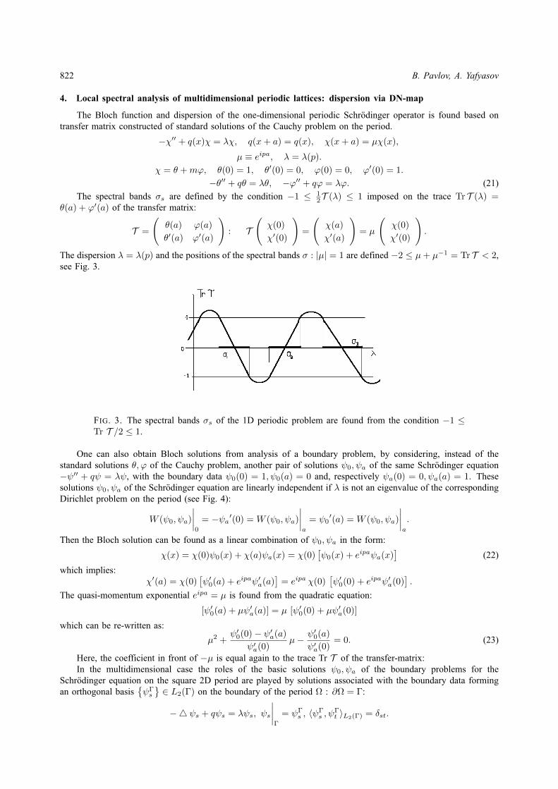
822 B. Pavlov, A. Yafyasov
4. Local spectral analysis of multidimensional periodic lattices: dispersion via DN-map
The Bloch function and dispersion of the one-dimensional periodic Schrodinger operator is found based ontransfer matrix constructed of standard solutions of the Cauchy problem on the period.
−χ′′ + q(x)χ = λχ, q(x+ a) = q(x), χ(x+ a) = µχ(x),
µ ≡ eipa, λ = λ(p).
χ = θ +mϕ, θ(0) = 1, θ′(0) = 0, ϕ(0) = 0, ϕ′(0) = 1.
−θ′′ + qθ = λθ, −ϕ′′ + qϕ = λϕ. (21)
The spectral bands σs are defined by the condition −1 ≤ 12T (λ) ≤ 1 imposed on the trace Tr T (λ) =
θ(a) + ϕ′(a) of the transfer matrix:
T =
(θ(a) ϕ(a)
θ′(a) ϕ′(a)
): T
(χ(0)
χ′(0)
)=
(χ(a)
χ′(a)
)= µ
(χ(0)
χ′(0)
).
The dispersion λ = λ(p) and the positions of the spectral bands σ : |µ| = 1 are defined −2 ≤ µ+ µ−1 = Tr T < 2,see Fig. 3.
FIG. 3. The spectral bands σs of the 1D periodic problem are found from the condition −1 ≤Tr T /2 ≤ 1.
One can also obtain Bloch solutions from analysis of a boundary problem, by considering, instead of thestandard solutions θ, ϕ of the Cauchy problem, another pair of solutions ψ0, ψa of the same Schrodinger equation−ψ′′ + qψ = λψ, with the boundary data ψ0(0) = 1, ψ0(a) = 0 and, respectively ψa(0) = 0, ψa(a) = 1. Thesesolutions ψ0, ψa of the Schrodinger equation are linearly independent if λ is not an eigenvalue of the correspondingDirichlet problem on the period (see Fig. 4):
W (ψ0, ψa)
∣∣∣∣0
= −ψa′(0) = W (ψ0, ψa)
∣∣∣∣a
= ψ0′(a) = W (ψ0, ψa)
∣∣∣∣a
.
Then the Bloch solution can be found as a linear combination of ψ0, ψa in the form:
χ(x) = χ(0)ψ0(x) + χ(a)ψa(x) = χ(0)[ψ0(x) + eipaψa(x)
](22)
which implies:χ′(a) = χ(0)
[ψ′0(a) + eipaψ′a(a)
]= eipa χ(0)
[ψ′0(0) + eipaψ′a(0)
].
The quasi-momentum exponential eipa = µ is found from the quadratic equation:
[ψ′0(a) + µψ′a(a)] = µ [ψ′0(0) + µψ′a(0)]
which can be re-written as:
µ2 +ψ′0(0)− ψ′a(a)
ψ′a(0)µ− ψ′0(a)
ψ′a(0)= 0. (23)
Here, the coefficient in front of −µ is equal again to the trace Tr T of the transfer-matrix:In the multidimensional case the roles of the basic solutions ψ0, ψa of the boundary problems for the
Schrodinger equation on the square 2D period are played by solutions associated with the boundary data formingan orthogonal basis
ψΓs
∈ L2(Γ) on the boundary of the period Ω : ∂Ω = Γ:
−4 ψs + qψs = λψs, ψs
∣∣∣∣Γ
= ψΓs , 〈ψΓ
s , ψΓt 〉L2(Γ) = δst.
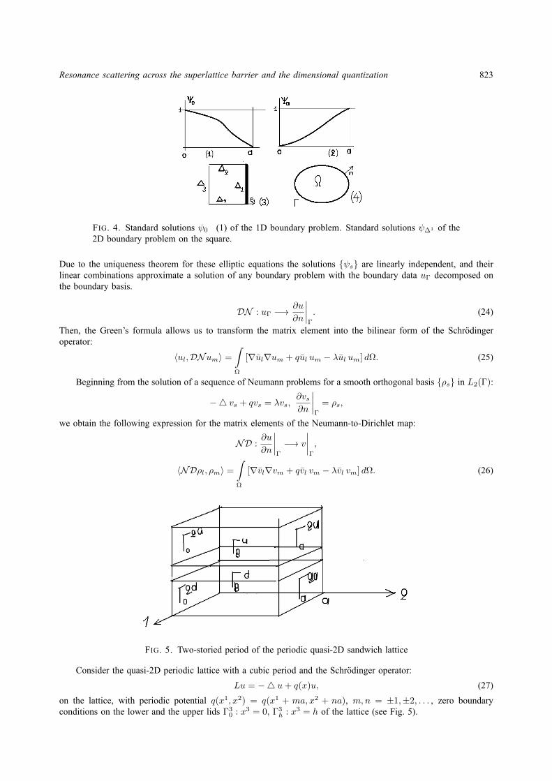
Resonance scattering across the superlattice barrier and the dimensional quantization 823
FIG. 4. Standard solutions ψ0 (1) of the 1D boundary problem. Standard solutions ψ∆1 of the2D boundary problem on the square.
Due to the uniqueness theorem for these elliptic equations the solutions ψs are linearly independent, and theirlinear combinations approximate a solution of any boundary problem with the boundary data uΓ decomposed onthe boundary basis.
DN : uΓ −→∂u
∂n
∣∣∣∣Γ
. (24)
Then, the Green’s formula allows us to transform the matrix element into the bilinear form of the Schrodingeroperator:
〈ul,DNum〉 =
∫Ω
[∇ul∇um + qul um − λul um] dΩ. (25)
Beginning from the solution of a sequence of Neumann problems for a smooth orthogonal basis ρs in L2(Γ):
−4 vs + qvs = λvs,∂vs∂n
∣∣∣∣Γ
= ρs,
we obtain the following expression for the matrix elements of the Neumann-to-Dirichlet map:
ND :∂u
∂n
∣∣∣∣Γ
−→ v
∣∣∣∣Γ
,
〈NDρl, ρm〉 =
∫Ω
[∇vl∇vm + qvl vm − λvl vm] dΩ. (26)
FIG. 5. Two-storied period of the periodic quasi-2D sandwich lattice
Consider the quasi-2D periodic lattice with a cubic period and the Schrodinger operator:
Lu = −4 u+ q(x)u, (27)
on the lattice, with periodic potential q(x1, x2) = q(x1 + ma, x2 + na), m,n = ±1,±2, . . . , zero boundaryconditions on the lower and the upper lids Γ3
0 : x3 = 0, Γ3h : x3 = h of the lattice (see Fig. 5).
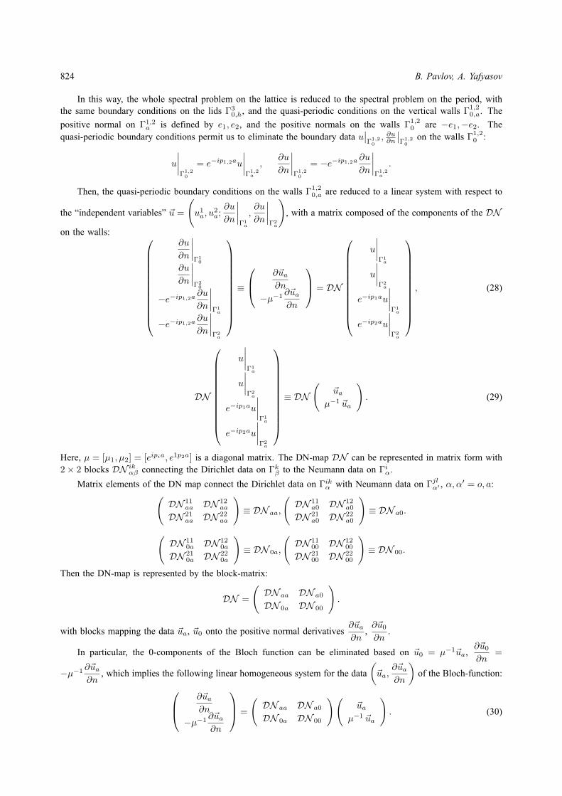
824 B. Pavlov, A. Yafyasov
In this way, the whole spectral problem on the lattice is reduced to the spectral problem on the period, withthe same boundary conditions on the lids Γ3
0,h, and the quasi-periodic conditions on the vertical walls Γ1,20,a. The
positive normal on Γ1,2a is defined by e1, e2, and the positive normals on the walls Γ1,2
0 are −e1,−e2. Thequasi-periodic boundary conditions permit us to eliminate the boundary data u
∣∣Γ1,2
0, ∂u∂n
∣∣Γ1,2
0on the walls Γ1,2
0 :
u
∣∣∣∣Γ1,2
0
= e−ip1,2au
∣∣∣∣Γ1,2a
,∂u
∂n
∣∣∣∣Γ1,2
0
= −e−ip1,2a∂u
∂n
∣∣∣∣Γ1,2a
.
Then, the quasi-periodic boundary conditions on the walls Γ1,20,a are reduced to a linear system with respect to
the “independent variables” ~u =
(u1a, u
2a;∂u
∂n
∣∣∣∣Γ1a
,∂u
∂n
∣∣∣∣Γ2a
), with a matrix composed of the components of the DN
on the walls:
∂u
∂n
∣∣∣∣Γ1
0
∂u
∂n
∣∣∣∣Γ2
0
−e−ip1,2a∂u
∂n
∣∣∣∣Γ1a
−e−ip1,2a∂u
∂n
∣∣∣∣Γ2a
≡
∂~ua∂n
−µ−1 ∂~ua∂n
= DN
u
∣∣∣∣Γ1a
u
∣∣∣∣Γ2a
e−ip1au
∣∣∣∣Γ1a
e−ip2au
∣∣∣∣Γ2a
, (28)
DN
u
∣∣∣∣Γ1a
u
∣∣∣∣Γ2a
e−ip1au
∣∣∣∣Γ1a
e−ip2au
∣∣∣∣Γ2a
≡ DN
(~ua
µ−1 ~ua
). (29)
Here, µ = [µ1, µ2] = [eipia, e1p2a] is a diagonal matrix. The DN-map DN can be represented in matrix form with2× 2 blocks DN ik
αβ connecting the Dirichlet data on Γkβ to the Neumann data on Γiα.
Matrix elements of the DN map connect the Dirichlet data on Γikα with Neumann data on Γjlα′ , α, α′ = o, a:(DN 11
aa DN 12aa
DN 21aa DN 22
aa
)≡ DN aa,
(DN 11
a0 DN 12a0
DN 21a0 DN 22
a0
)≡ DN a0.
(DN 11
0a DN 120a
DN 210a DN 22
0a
)≡ DN 0a,
(DN 11
00 DN 1200
DN 2100 DN 22
00
)≡ DN 00.
Then the DN-map is represented by the block-matrix:
DN =
(DN aa DN a0
DN 0a DN 00
).
with blocks mapping the data ~ua, ~u0 onto the positive normal derivatives∂~ua∂n
,∂~u0
∂n.
In particular, the 0-components of the Bloch function can be eliminated based on ~u0 = µ−1~ua,∂~u0
∂n=
−µ−1 ∂~ua∂n
, which implies the following linear homogeneous system for the data
(~ua,
∂~ua∂n
)of the Bloch-function: ∂~ua
∂n
−µ−1 ∂~ua∂n
=
(DN aa DN a0
DN 0a DN 00
)(~ua
µ−1 ~ua
). (30)
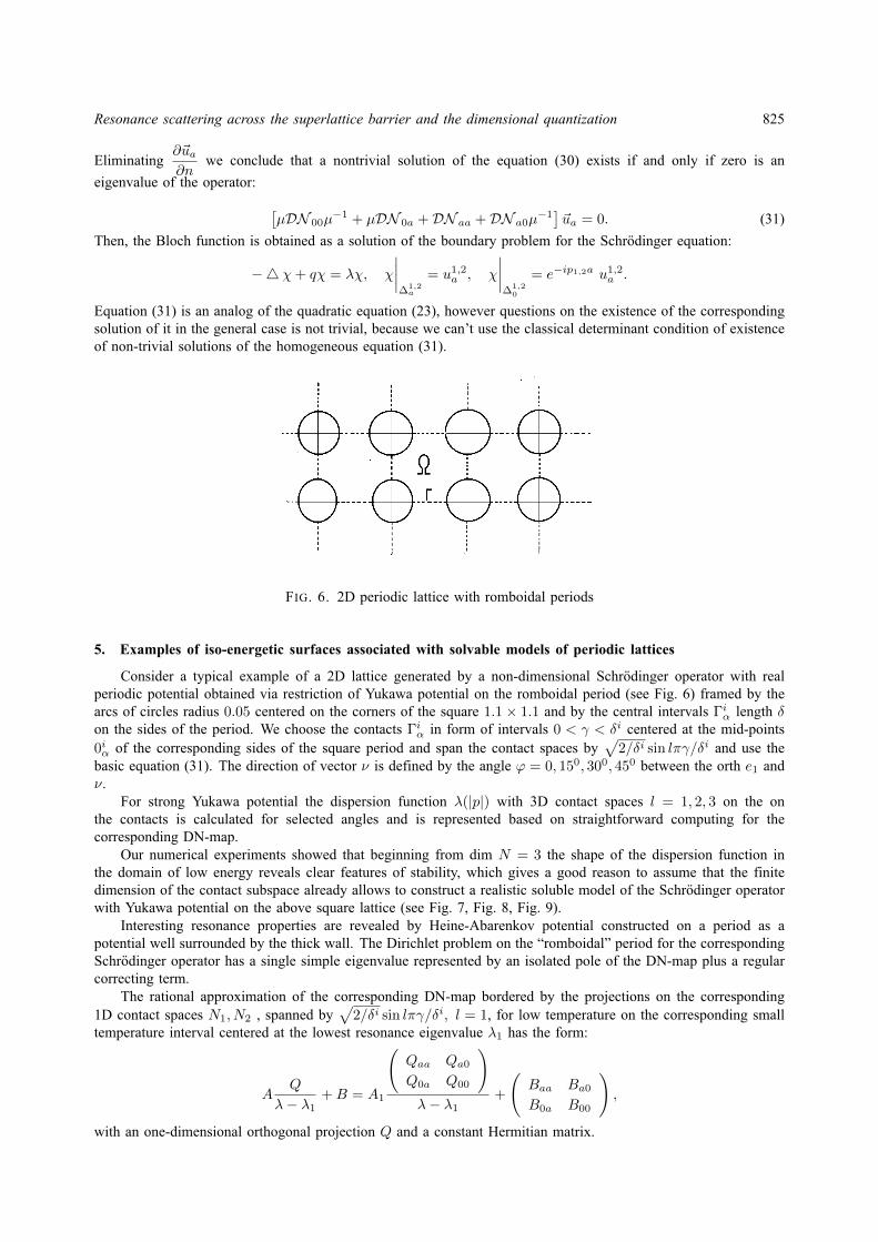
Resonance scattering across the superlattice barrier and the dimensional quantization 825
Eliminating∂~ua∂n
we conclude that a nontrivial solution of the equation (30) exists if and only if zero is an
eigenvalue of the operator: [µDN 00µ
−1 + µDN 0a +DN aa +DN a0µ−1]~ua = 0. (31)
Then, the Bloch function is obtained as a solution of the boundary problem for the Schrodinger equation:
−4 χ+ qχ = λχ, χ
∣∣∣∣∆1,2
a
= u1,2a , χ
∣∣∣∣∆1,2
0
= e−ip1,2a u1,2a .
Equation (31) is an analog of the quadratic equation (23), however questions on the existence of the correspondingsolution of it in the general case is not trivial, because we can’t use the classical determinant condition of existenceof non-trivial solutions of the homogeneous equation (31).
FIG. 6. 2D periodic lattice with romboidal periods
5. Examples of iso-energetic surfaces associated with solvable models of periodic lattices
Consider a typical example of a 2D lattice generated by a non-dimensional Schrodinger operator with realperiodic potential obtained via restriction of Yukawa potential on the romboidal period (see Fig. 6) framed by thearcs of circles radius 0.05 centered on the corners of the square 1.1× 1.1 and by the central intervals Γiα length δon the sides of the period. We choose the contacts Γiα in form of intervals 0 < γ < δi centered at the mid-points0iα of the corresponding sides of the square period and span the contact spaces by
√2/δi sin lπγ/δi and use the
basic equation (31). The direction of vector ν is defined by the angle ϕ = 0, 150, 300, 450 between the orth e1 andν.
For strong Yukawa potential the dispersion function λ(|p|) with 3D contact spaces l = 1, 2, 3 on the onthe contacts is calculated for selected angles and is represented based on straightforward computing for thecorresponding DN-map.
Our numerical experiments showed that beginning from dim N = 3 the shape of the dispersion function inthe domain of low energy reveals clear features of stability, which gives a good reason to assume that the finitedimension of the contact subspace already allows to construct a realistic soluble model of the Schrodinger operatorwith Yukawa potential on the above square lattice (see Fig. 7, Fig. 8, Fig. 9).
Interesting resonance properties are revealed by Heine-Abarenkov potential constructed on a period as apotential well surrounded by the thick wall. The Dirichlet problem on the “romboidal” period for the correspondingSchrodinger operator has a single simple eigenvalue represented by an isolated pole of the DN-map plus a regularcorrecting term.
The rational approximation of the corresponding DN-map bordered by the projections on the corresponding1D contact spaces N1, N2 , spanned by
√2/δi sin lπγ/δi, l = 1, for low temperature on the corresponding small
temperature interval centered at the lowest resonance eigenvalue λ1 has the form:
AQ
λ− λ1+B = A1
(Qaa Qa0
Q0a Q00
)λ− λ1
+
(Baa Ba0
B0a B00
),
with an one-dimensional orthogonal projection Q and a constant Hermitian matrix.
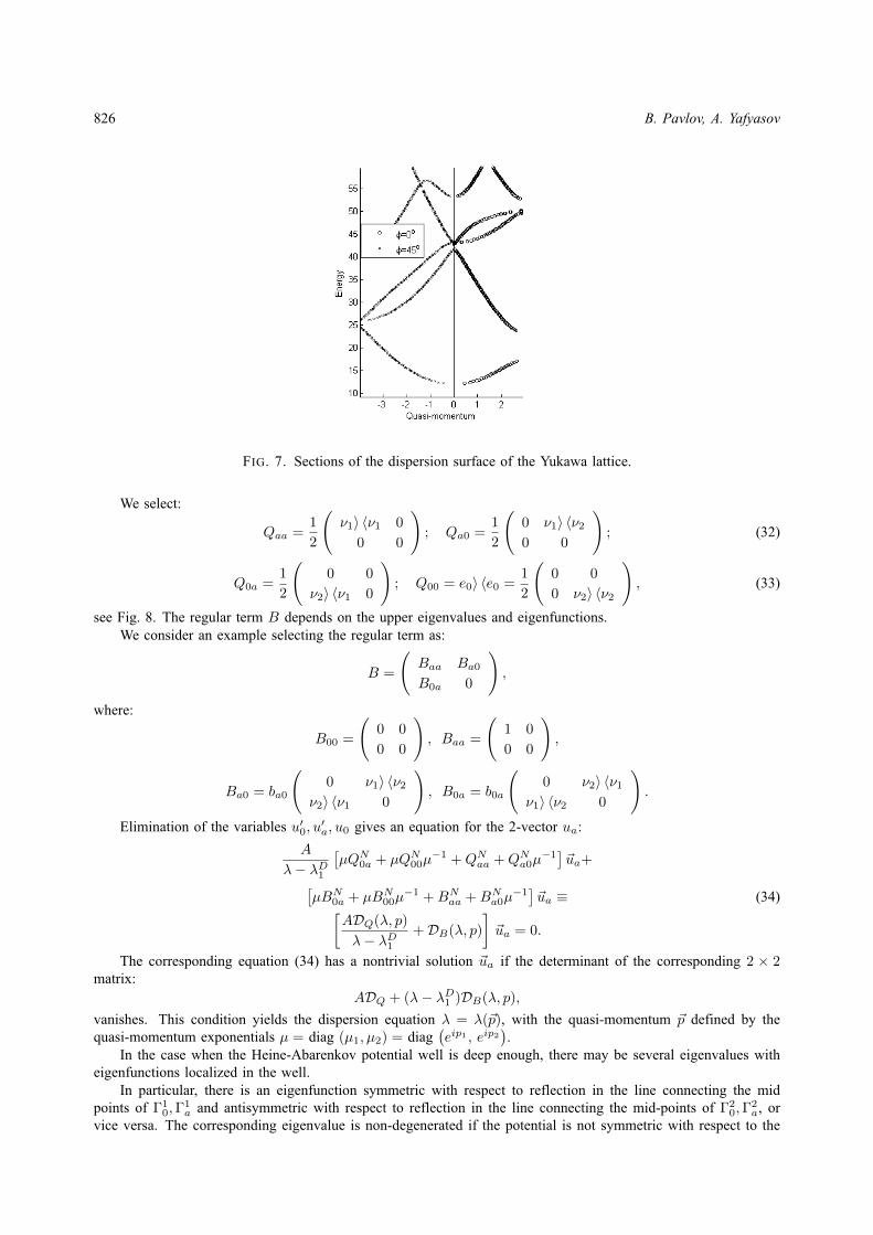
826 B. Pavlov, A. Yafyasov
FIG. 7. Sections of the dispersion surface of the Yukawa lattice.
We select:
Qaa =1
2
(ν1〉 〈ν1 0
0 0
); Qa0 =
1
2
(0 ν1〉 〈ν2
0 0
); (32)
Q0a =1
2
(0 0
ν2〉 〈ν1 0
); Q00 = e0〉 〈e0 =
1
2
(0 0
0 ν2〉 〈ν2
), (33)
see Fig. 8. The regular term B depends on the upper eigenvalues and eigenfunctions.We consider an example selecting the regular term as:
B =
(Baa Ba0
B0a 0
),
where:
B00 =
(0 0
0 0
), Baa =
(1 0
0 0
),
Ba0 = ba0
(0 ν1〉 〈ν2
ν2〉 〈ν1 0
), B0a = b0a
(0 ν2〉 〈ν1
ν1〉 〈ν2 0
).
Elimination of the variables u′0, u′a, u0 gives an equation for the 2-vector ua:
A
λ− λD1
[µQN0a + µQN00µ
−1 +QNaa +QNa0µ−1]~ua+[
µBN0a + µBN00µ−1 +BNaa +BNa0µ
−1]~ua ≡ (34)[
ADQ(λ, p)
λ− λD1+DB(λ, p)
]~ua = 0.
The corresponding equation (34) has a nontrivial solution ~ua if the determinant of the corresponding 2 × 2matrix:
ADQ + (λ− λD1 )DB(λ, p),
vanishes. This condition yields the dispersion equation λ = λ(~p), with the quasi-momentum ~p defined by thequasi-momentum exponentials µ = diag (µ1, µ2) = diag
(eip1 , eip2
).
In the case when the Heine-Abarenkov potential well is deep enough, there may be several eigenvalues witheigenfunctions localized in the well.
In particular, there is an eigenfunction symmetric with respect to reflection in the line connecting the midpoints of Γ1
0,Γ1a and antisymmetric with respect to reflection in the line connecting the mid-points of Γ2
0,Γ2a, or
vice versa. The corresponding eigenvalue is non-degenerated if the potential is not symmetric with respect to the
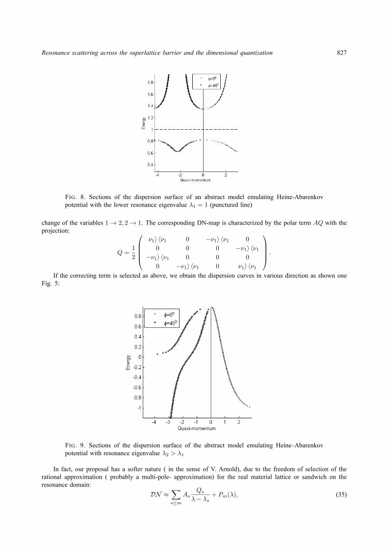
Resonance scattering across the superlattice barrier and the dimensional quantization 827
FIG. 8. Sections of the dispersion surface of an abstract model emulating Heine-Abarenkovpotential with the lower resonance eigenvalue λ1 = 1 (punctured line)
change of the variables 1→ 2, 2→ 1. The corresponding DN-map is characterized by the polar term AQ with theprojection:
Q =1
2
ν1〉 〈ν1 0 −ν1〉 〈ν1 0
0 0 0 −ν1〉 〈ν1
−ν1〉 〈ν1 0 0 0
0 −ν1〉 〈ν1 0 ν1〉 〈ν1
.
If the correcting term is selected as above, we obtain the dispersion curves in various direction as shown oneFig. 5:
FIG. 9. Sections of the dispersion surface of the abstract model emulating Heine–Abarenkovpotential with resonance eigenvalue λ2 > λ1
In fact, our proposal has a softer nature ( in the sense of V. Arnold), due to the freedom of selection of therational approximation ( probably a multi-pole- approximation) for the real material lattice or sandwich on theresonance domain:
DN ≈∑s≤m
AsQs
λ− λs+ Pm(λ), (35)
828 B. Pavlov, A. Yafyasov
the choice of the contacts/contact subspaces and temperature (interval of admissible values of energy). We speculatethat this problem, although it appears to be a mathematical one, lies outside of mathematics, on the interface withquantum chemistry, with its specific system of notions (covalent bonds, etc...) and methods.
.
Appendix 1: Lagrangian version of the operator extension algorithm
John von Neumann – nearly 90 years ago – tried to attract attention of physicists to the basic differencebetween symmetric and self-adjoint operators, see [18], and proposed a geometrical solution to the most importantproblem of construction of a self-adjoint extension of a symmetric operator. Unfortunately, this solution was not,at that time, properly recognized by physicists. A few years later, E. Fermi, attempting to describe scattering ofneutrons by nuclei, considered the Laplacian on a domain of smooth L2(R3) functions with typical singularity at
the origin u =Au
4π|x|+Bu +O(|x|) and discovered that the boundary form of the Laplacian:
J(u, v) = limδ→0
∫|x|>δ
[−∆uv + u∆v] d3x = AuBv − BuAv (36)
vanishes under the boundary condition B = γA with real γ. Later probably used another approach to the problemof extending of a symmetric operator to the corresponding self-adjoint, which yields a convenient formula forthe scattered waves, see [19]. Though the conventional proof of self-adjointness of the Laplacian under theabove boundary conditions was proposed 25 years later, see [20], the approach to operator extension based onthe boundary form proved to be extremely efficient, see for instance [12, 13, 21] 1In 1970’s, it was modifiedby introducing the inner structure into zero-range potential, see [12, 13], that allowed consideration of resonanceinteraction, which allows admission of fitting based on asymptotics Dirichlet-to-Neumann map of the correspondingunperturbed problem, see [22]. This approach allows one to develop an analytic perturbation technique forembedded eigenvalues, based on two step analytic perturbation procedure - a quantum Jump-Start analog of thecorresponding classical techniques developed by Poincare [23] and, in particular, to propose a convenient solvablemodel for Quantum Networks, supplied with inner structure on the nodes, see [24] 2.
Hereafter, we produce a brief review of the Lagrangian operator extension techniques for an abstract operator,presenting the corresponding symplectic boundary form in terms of appropriate analog of boundary values, andimposing the corresponding boundary conditions, to select a domain of the relevant self-adjoint extension as aLagrangian plane of the symplectic boundary form.
Consider a finite Hermitian matrix A in a finite-dimensional Hilbert space A : K → K, dim K = k. Select
a deficiency subspace Ni ∈ K, dim Ni < k/2, such that does not overlap with N−i =A+ iI
A− iINi and consider
the restriction A0 = A
∣∣∣∣D0
onto the subspace D0 ≡ (A − iI)−1 [K Ni]. The restricted operator is not densely
defined, but its formal adjoint can be defined by J. von Neumann formulae on the defect N = Ni + N−i asA+ni + ini = 0, ni ∈ Ni, A+n−i − in−i = 0, n−i ∈ N−i, see [25], where the operator extension procedure isdeveloped for A0. In [12,13], see also references therein, a simplectic version of the operator extension procedurewas proposed for A0, which is convenient for manufacturing zero-range perturbations with inner structure fordifferential operators, see for instance [12, 13, 24]. In particular, a quantum dot attached to the star-graph Γ = ∪γlis modeled in [24] based on zero-range potential with inner structure while reducing L → L0 the Schrodingeroperator by the condition of vanishing elements of the domain D(L0) near the knot x = 0 of the star, such that theadjoint opeartor L+
0 has the boundary form represented as a sum over all branches γl of the star graph Γ, meetingat the node x = 0:
Jext(u, v) =∑l
∫γl
[−u”
l vl + ulv”l
]dx =
∑l
[−u′lvl + ulv′l]
∣∣∣∣0
, (37)
1I. M. Gelfand attracted attention of mathematicians to importance of development a Lagrangian approach to operator extensions, basedon selecting a Lagrangian plane in the domain of the adjoint operator, which would serve an alternative to the J. von Neumann geometricalconstruction, [26].
2Notice, that I. Prigogine in 1973 formulated the hypothesis on the validity of the Poincare two-step algorithm of analytic perturbationprocedure for quantum problems, see [27], but could not prove it, because selected an incorrect anzsatz was selected for the correspondingIntermediate operator. The hypothesis was later proved for Quantum Networks based on the correct ansatz, [22], for the intermediate operator,presented in the form of zero-range model with an inner structure, constructed with use of Lagrangian technique of operator extensionprocedure [23]
Resonance scattering across the superlattice barrier and the dimensional quantization 829
with differentiation in an outgoing direction at the node. The boundary form of the inner Hamiltonian A iscalculated in a special representation of the boundary form J int(u, v), constructed based on an orthogonal basisel ⊂ Ni:W l
+
=
1
2
[el +
A+ iI
A− iIel
]=
A
A− iIel
and
W l−
=
1
2
[el −
A+ iI
A− iIel
]=
− 1
A− iIel
. (38)
Jext(u, v) =∑l
∫γl
[−u”
l vl + ulv”l
]dx =
∑l
[−u′lvl + ulv′l]
∣∣∣∣0
, (39)
with differentiation in an outgoing direction at the node. The boundary form of the inner Hamiltonian A iscalculated in a special representation of the boundary form J int(u, v), constructed based on an orthogonal basisel ⊂ Ni:W l
+
=
1
2
[el +
A+ iI
A− iIel
]=
A
A− iIel
and
W l−
=
1
2
[el −
A+ iI
A− iIel
]=
− 1
A− iIel
. (40)
Then, each element from the defect N = Ni + N−i can be represented as u =∑l
A
A− iIξl+ −
1
A− iIξl− ≡
A
A− iI~ξu+−
1
A− iI~ξu−, and the vectors ~ξu± ∈ Ni play roles of the boundary data. The boundary form of the formal
adjoint operator A+0 is calculated on elements u, v ∈ N from the defect as:
J int(u, v) = 〈A+u, v〉 − 〈u,A+v〉 = 〈~ξu+, ~ξv−〉 − 〈~ξu−, ~ξv+〉. (41)
The ultimate formula is valid tot only on the defect, but on the whole space K = D0 +N with A+0 extended from
N onto D0 as A0, that is , for u = u0 + uN :
A+(u0 + uN ) = A0u0 +A+0 uN ,
so that the addendum A0u0 does not contribute to the boundary form Jext(u, v), and Jext(u, v) = 〈A+uN , vN 〉 −〈uN , A+vN 〉. In particular, the boundary data ξu± for a solution of the homogeneous adjoint equation:
A+(u0 + uN )− λ(u0 + uN ) = 0
are connected by the Krein function M(λ) = PNi
I + λA
A− λI
∣∣∣∣Ni
as:
ξu− + PNi
I + λA
A− λI
∣∣∣∣Ni
ξu+ = 0. (42)
A self-adjoint extension of the restricted operator A0 on the defect is constructed as a part of the extendedadjoint operator onto the Lagrangian plane NB in the defect, submitted to the boundary condition:
~ξu− +B~ξu+ = 0, (43)
with an Hermitian operator B : Ni → Ni The boundary form (41) vanishes on the plane. Then, the correspondingself-adjoint extension of an original restricted operator A0 is defined as a sum A0 + AB acting according to thevon Neumann formulae respectively in D0 and in NB ⊂ N on elements:
u = u0 +A
A− iI~ξu+ −
I
A− iI~ξu−
with the boundary values connected by the above boundary conditions .The spectrum of the extension is defined by the Krein function:
PNi
I + λA
A− λIPNi ≡M(λ), (44)
which connects the boundary values ~ξu± of the solution u of the homogeneous adjoint equation A+u− λu = 0:
~ξu− +M(λ)~ξu+ = 0. (45)
and the spectrum of the extension AB is defined by the singularities of the corresponding ratio
I
B −M(λ), (46)
830 B. Pavlov, A. Yafyasov
which serves the inner factor in the Krein formula for the resolvent of the extension:I
AB − λI=
I
A− λI+A+ iI
A− λIPNi
I
B −M(λ)PNi
A− iIA− λI
. (47)
Appendix 2: Solvable models of selected one-body spectral problems
In this section we construct a one-body model of a quantum dot Ω attached to the node of a 1D quantumstar-graph Γ = Γ1 ∪ Γ2 ∪ Γ3 . . .Γn and a one-body model of 1D periodic chain. Despite selection of simplestalgebraic parameters for the corresponding solvable models, they have rich spectral propeties which can be easilymonitored due to the algebraic nature of the parameters selected. Both models are constructed via Lagrangianversion of the operator extension procedure, with regard of the symplectic boundary forms J balancing to zero onLagrangian planes, selected based on the corresponding boundary conditions.
Quantum dot attached to the node of a quantum graph
On a star-graph Γ = Γ1 ∪ Γ2 ∪ Γ3 . . .Γn of straight shoulders Γs attached to a compact domain Ω with asmooth boundary, we consider a spectral problem for a the 1D Schrodinger equation LΓ = −~u′′
Γ in L2(Γ, EΓ) withEΓ = Cn, with regard of appropriate boundary condition connecting it with the Schrodinger operator LΩuΩ =−∆uΩ + V uΩ on the domain Ω supplied with the zero boundary condition L2(∂Ω) EΩ. A bond B is imposedon the contact EΩ × EΓ with the projection PΩ ≡ PEΩ . This was done with the consideration of the boundaryforms calculated on both sides of the contact Γ ∩ ∂Ω in the corresponding contact subspaces Cn = EΓ, EΩ, withPΩ ≡ P
EΩ :
JΓ(uΓ, vΓ) ≡ 〈~u′Γ, ~vΓ〉 − 〈~uΓ, ~v′Γ〉, JΩ(uΩ, vΩ) ≡ −〈∂uΩ
∂n, PΩvΩ〉+ 〈PΩuΩ,
∂vΩ
∂n〉, (48)
and a boundary condition imposed with an Hermitian matrix:
B =
(0 beibie aii
),
(~u′Γ
−PΩ ∂uΩ
∂n
)+B
(~uΓ
PΩuΩ
)= 0, (49)
with an Hermitian operator aii : EΩ → EΩ and bei : EΩ → EΓ, bie = b+ei. We denote by M ≡ −PΩDNPΩ =∑l
PΩ ∂ϕl
∂n 〉〈∂ϕl
∂n PΩ
λl − λthe framed DN-map 3 of the quantum dot:
−∆uΩ + V uΩ = λuΩ, DN : uΩ →∂uΩ
∂n
∣∣∣∣∂Ω
,
and rewrite equation (49), for the scattering Ansatz eipx~e+ e−ipxS~e = ~u, p2 = λ:
ip(I − S)e+ beiPΩuΩ = 0
[M+ aii]PΩuΩ+ bie(I + S)e = 0.
(50)
Eliminating PΩuΩ and introducing bei 1M+aii
bie ≡ N b(λ), we obtain an expression for the scattering matrix:
S(p) =ip−N b
ip+N b, with =N b =λ > 0, (51)
in terms of the framed Neumann-to-Dirichlet map N b.Though the Dirichlet-to-Neumann map of the 3D domain Ω can be computed with standard programs, see
for instance [28], yet it is also convenient to substitute it by perturbation analysis [] using finite-dimensionalapproximation, taking into account only a finite number of eigenvalues λl or substituting the quantum dot byzero-range potential with inner structure, see [12,13]. In particular, for a 1D framed DN map, the framed ND-mapN b ≡ bei 1
M+aiibie has generally has asymptotes at infinity λ→∞:
N b(λ) = Aλ+ A0 +
k∑l=1
Alλl − λ
, (52)
with A ≥ 0, A0 = A0, Al ≥ 0. It is possible to select a finite-dimensional self-adjoint operator A : K → Kand an interaction B, with non-overlapping deficiency subspaces Ni, N−i such that, being attached to node of the
3The above formal series is actually divergent, but may be properly regularized, see for instance [29].
Resonance scattering across the superlattice barrier and the dimensional quantization 831
above star-graph Γ, plays a role of an inner Hamiltonian of a quantum dot with the scattering matrix (51) on thestar-graph, with the boundary conditions .
A solvable model of a discrete lattice
Consider a 1D periodic lattice ( a chain) of equivalent quantum dots Ω ≡ Ωl arising of equivalent finite-dimensional operators Al ≡ A : Kl → Kl, with equivalent non-overlapping 1D deficiency subspaces N l
i , Nl−i.
Each quantum dot is substituted by the zero-range potential with an inner structure as described in Appendix 1:
ξ+ ∼ PEuΩ
∣∣∣∣Γ
, ξ− ∼ −PE∂uΩ
∂n
∣∣∣∣Γ
, ξ− +Mξ+ = 0, (53)
and a pair of infinite-dimensional vectors ~ξ+ =∑l ξl−,
~ξ− =∑l ξl+, which play a role of the boundary values
for the whole chain. We choose the simplest translation - invariant boundary conditions, connecting the nearestneighbors in the chain as:
ξl− + b+ ξl−1+ + b0 + b ξl+1
+ = 0, or, alternativelyξl+ + c− ξl−1− + c0 + c ξl+1
− = 0. (54)
Denoting the sequence ξl shifted one step to the left as T+~ξ =ξl+1
and, similarly the sequence shifted one step
to the right T ~ξ =ξl−1
, we represent the above boundary conditions respectively as:
~ξ− +[b+T+ + b0 + bT
]~ξ+ = 0 ≡ ~ξ− +B~ξ+,
~ξ+ +[c+T+ + c0 + cT
]~ξ+ = 0 ≡ ~ξ+ + C~ξ−, (55)
Regarding the periodicity of the chain of quantum dots, the corresponding sequences of their Weyl-Titchmatsh orKrein finctions diag M≡ ⊕
∑Ml are also periodics:
T+diagMT = TdiagMT+ = diagM.
With 1D contact subspaces El ≡ E and the interaction B or C between the boundary data on the chain, the bound-ary values of the relevant Bloch functions ~Ξ are quasi-periodic Ξl± = eipl Ξ0
±, with regard to the quasimomentump:
MΞ0+ −
[b+e−ip + b0 + beip
]Ξ0
+ = 0, for the boundary codition B, and
Ξ0+ −M
[c+e−ip + c0 + ceip
]Ξ0
+ = 0 (56)
for the boundary condition C. In the case of the quantum dot substituted by the zero-range boundary conditionwith an inner structure, as in Appendix 1:
M = PEI + λA
A− λIPE = −PEAPE + PE
I +A2
A− λIPE ≈ −PEAPE −
PE(I +A2)PEλ
+O(1/λ)2 (57)
For a special choice of the boundary parameters −PEAPE = b0 with regards to M+ b0 → 0 or, correspondingly,c0PEAPE = 1 with regards to I +Mc0 → 0 while λ → ∞, we get for the special choice of the boundaryparameters:
PAI +A2
A− λPEΞ0
+ + 2|b| cos(p+ ϕb)Ξ0+ = 0, (58)
and correspondingly:
(I + c0PEAPE) Ξ0+ − PE
(I +A2)
A− λIPE2|c| cos(p+ ϕc)Ξ
0+ = 0. (59)
The Nevanlinna function PA(I+A2)A−λ PE is invertible on real axis, and the innverse is also a Nevanlinna function
arising from a pair E,G with a finite-dimensional operator G : K → K with selected deficiency subspace Ni = E4
−[PE
(I +A2)
A− λPE
]−1
= λ[PE(I +A2)PE
]−1 − PEGPE + PEI +G2
G− λIPE , (60)
hence first addendum in (59) multiplied by[PE
(I+A2)A−λ PE
]−1
yields:
(I + c0PEAPE)
[λ[PA(I +A2)PE
]−1Ξ0
+ − PEGPE + PEI +G2
G− λIPE
]Ξ0
+. (61)
4The operators A and G are connected similarly to Laplacean with Dirichlet and Neumann boundary conditions on a domain with a smoothboundary.
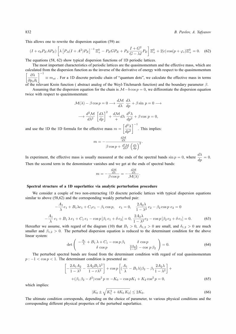
832 B. Pavlov, A. Yafyasov
This allows one to rewrite the dispersion equation (59) as:
(I + c0PEAPE)
[λ[PA(I +A2)PE
]−1Ξ0
+ − PEGPE + PEI +G2
G− λIPE
]Ξ0
+ + 2|c| cos(p+ ϕc)Ξ0+ = 0. (62)
The equations (58, 62) show typical dispersion functions of 1D periodic lattices.The most important characteristics of periodic lattices are the quasimomentum and the effective mass, which are
calculated from the dispersion function as the inverse of the derivative of energy with respect to the quasimomentum[∂λ
∂ps∂t
]−1
≡ mst . For a 1D discrete periodic chain of “quantum dots”, we calculate the effective mass in terms
of the relevant Krein function ( abstract analog of the Weyl-Titchmarsh function) and the boundary parameter β.Assuming that the dispersion equation for the chain isM−b cos p = 0, we differentiate the dispersion equation
twice with respect to quazimomentum:
M(λ)− β cos p = 0 −→ dMdλ
dλ
dp+ β sin p = 0 −→
−→ d2Mdλ2
[dλ
dp
]2
+dM+
dλd2λ
dp2+ β cos p = 0,
and use the 1D the 1D formula for the effective mass m =
[d2λ
dp2
]−1
. This implies:
m = −dMdλ
β cos p+ d2Mdλ2
(dλdp
)2 .
In experiment, the effective mass is usually measured at the ends of the spectral bands sin p = 0, wheredλ
dp= 0.
Then the second term in the denominator vanishes and we get at the ends of spectral bands:
m = −dMdλ
β cos p= −
dMdλ
M(λ).
Spectral structure of a 1D superlattice via analytic perturbation procedure
We consider a couple of two non-enteracting 1D discrete periodic lattices with typical dispersion equationssimilar to above (58,62) and the corresponding weakly perturbed pair:
−A1
λe1 +B1λe1 + C1e1 − β1 cos p, e1 = 0,
2A2λ
1− λ2e2 − β2 cos p e2 = 0
−A1
λe1 +B1 λ e1 + C1 e1 − cos p [β1 e1 + δ e2] = 0,
2A2λ
1− λ2e2 − cos p [β2 e2 + δ e1] = 0. (63)
Hereafter we assume, with regard of the diagram (10) that B1 > 0, A1,2 > 0 are small, and δ1,2 > 0 are muchsmaller and β1,2 > 0. The perturbed dispersion equation is reduced to the determinant condition for the abovelinear system:
det
(−A1
λ +B1 λ+ C1 − cos p β1 δ cos p
δ cos p 2A2λ1−λ2 − cos p β2
)= 0. (64)
The perturbed spectral bands are found from the determinant condition with regard of real quasimomentump : −1 < cos p < 1. The determinant condition is presented as:[
−2A1A2
1− λ2− 2A2B1λ
2
1− rλ2
]+ cos p
[(A1
λ−B1λ)β2 − β1
2A2λ
1− λ2
]+
+(β1 β2 − δ2) cos2 p ≡ −K0 − cos pK1 +K2 cos2 p = 0, (65)
which implies:
|K0 ±√K2
1 + 4K0K2| ≤ 2K0. (66)
The ultimate condition corresponds, depending on the choice of parameter, to various physical conditions and thecorresponding different physical properties of the perturbed superlattice.
Resonance scattering across the superlattice barrier and the dimensional quantization 833
FIG. 10. The spectral structure of the perturbed superlattice with regards to quasi-crossingsof terms of the underlying unperturbed lattices. The typical quasi-crossing for terms of theNevanlinna-class dispersion equations. The unperturbed spetral bands are shown as thin rectanglesmarked by numbers 1, 2
Acnowledgements
The autors are grateful to V. B. Bogevolnov for providing extremely interesting and inspiring material – thecarbon flakes obtained by detonation – which served main object of our experimental and the theoretical study.We are also grateful to Prof. G. Fursey, Prof. P. Konorov, Prof. P. Schwerdtfegger and Dr. Krista Steenbergen foran inspirating discussion of the mathematical analog of the shaky concept of chemical bound with respect to theproblem of selection appropriate contact subspaces for fitted solvable models of periodic lattices.
References
[1] Fursey G.N. Field emission in vacuum microelectronics. Kluwer Academic/Plenum Publishers (now Springer), New York, 2005.[2] Fursey G., Konorov P., Pavlov B. and Adil Yafyasov. Dimensional Quantization and the Resonance Concept of the Low-Threshold Field
Emission, Electronics, 2015, 4, P. 1101–1108.[3] Yafyasov A., Bogevolnov V., Fursey G., Pavlov B., Polyakov M., Ibragimov A. Low-threshold field emission from carbon nano-clusters.
Ultramicroscopy, 2011, 111, P. 409–414.[4] Bonard J-M., Stockli T., Majer F., W. de Heer, Chtelain A., Salvetat J-P., Forro L. Field-emission-Induced luminiscence from Carbon
Nanotubes. Phys. Rev. Letters, 81, 7–17 August 1998, P. 1441–1444.[5] Modinos A., Xanthakis J.P. Electron emission from amorphous carbon nitride film. Applied Physics Letters, Sept. 1998, 73,(13), P. 28.[6] Forbes G., Xanthakis J.P. Field penetration into amorphous-carbon films: consequences for field-induced electron emission. Surf. Interface
Anal.,2007, 39, P. 139–145.[7] Fursey G., Polyakov M., Pavlov B., Yafyasov A., Bogevolnov V. Exceptionally low Threshold of Field Emission from carbon nano-
clusters. Extended abstract. 24 International Vacuum Nanoelectronics conference. Bergishe Universitat, Wuppertal, Germany, 18–22 July2011.
[8] Flugge S. Practical Quantum Mechanics I, Ch.2. Springer Verlag, Heidelberg, new York, 1974, xvi, 331 p.[9] Datta S., Das Sarma B. Electronic analog of the electro-optic modulator. Appl. Phys. Lett., 1990, 56(7), P. 665–667.
[10] Shelykh I.A., Galki N.G.n, Bagraev N.T. Quantum splitter controlled by Rashba spin-orbit coupling. Phys. Rev.B, 2005, 72, P. 235316.[11] Harmer M., Pavlov B., Yafyasov A. Boundary condition at the junction. Journal of computational electronics, 2007, 6, P. 153–157.[12] Pavlov B. The theory of extensions and explicitly solvable models. (In Russian) Uspekhi Mat. Nauk, 1987, 42, P. 99–131.[13] Pavlov B. A solvable model for scattering on a junction and a modified analytic perturbation procedure. Operator theory: Advances and
Applications, 2009, 197, P. 281–335. Birkhauser, Basel/Switzerland.[14] Bagraev N.T. Metastable surface defects in p-type Ga As. Materials Science Forum vols, 1994, 143-147, P. 543–548.[15] Davies J.H. The Physics of Low-Dimensional Semiconductor. An Introduction, Cambridge University. Press: Cambridge, UK, 1998, P. 438.[16] Fursey G.N., Egorov N.V., Zakirov I.I., et al. Peculiarities of the total energy disribution of the field emission electrons from graphene-like
structures: Distribution on full energy. Radiotechnika i electronika., 2015, 6,11, P. 1–4. (in press) (In Russian).[17] Karpeshina Yu.E. Spectrum and Eigenfunctions of the Schrodinger operator in a three-dimensional space with periodic point potential of
two-dimensional lattice type. In Russian TMF, 1983, 57(3), P. 414–423.[18] von Neumann J. Mathematical foundations of quantum mechanics. Twelfth printing. Princeton Landmarks in Mathematics. Princeton
Paperbacks. Princeton University Press, Princeton, NJ, 1996.[19] Fermi E. Sul motto del neutroni nelle sostanze idrigenante. Ricerca Sci., 1936, P. 13–52.[20] Berezin F.A.,Faddeev L.D. A remark on the Schrodinger equation with with a singular potential. Soviet Math. Doklady, 1961, 2, P. 372–376.

834 B. Pavlov, A. Yafyasov
[21] Albeverio S. and Kurasov P. Singular Perturbations of Differential Operators. Solvable Schrodinger Type Operators. London MathematicalSociety Lecture Note Series vol 271, Cambridge University Press, 2000, xiv+429 p.
[22] Bagraev N., Mikhailova A., Pavlov B., Prokhorov L., Yafyasov A. Parametric regimes of a resonance quantum switch. Phys. Rev. B, 2005,71, P. 165308.
[23] Pavlov B., Antoniou I. Jump-start in the analytic perturbation procedure for the Friedrichs model. J. Phys. A (Math. Gen), 2005, 38,P. 4811–4823.
[24] Pavlov B. A star-graph model via operator extension. Mathematical Proceedings of the Cambridge Philosophical Society, 2007, 142(02),P. 365–384.
[25] Krasnoselskij M.A. On selfadjoint extensions of Hermitian Operators. (in Russian) Ukrainskij Mat.Journal, 1949, 1(21), P. 21–38.[26] S.P. Novikov private communication 2012, MIAN.[27] Prigogine I. Irreversibility as a symmetry-breacking process. Nature, 1976, 246, P. 9.[28] Martin G., Pavlov B., Yafyasov A. Resonance one-body scattering on a junction. Nanosystems: Physics, Chemistry, Mathematics, 2010,
1(1), P. 108–147.[29] Pavlov B. S-Matrix and Dirichlet-to-Neumann Operators. Scattering and Semigroup Theory. In: Scattering, ed. R.Pike, P. Sabatier,
Academic Press, Harcourt Science and Tech. Company. 2000, P. 1678–1688.
NANOSYSTEMS: PHYSICS, CHEMISTRY, MATHEMATICS, 2016, 7 (5), P. 835–841
Control and inverse problems for networks of vibrating stringswith attached masses
F. Al-Musallam1, S. Avdonin2, N. Avdonina2, J. Edward3
1Department of Mathematics, Kuwait University, P.O Box 5969 Safat, Kuwait2Department of Mathematics and Statistics, University of Alaska, Fairbanks, AK 99775, USA
3Department of Mathematics and Statistics, Florida International University, Miami, FL 33199, USA
[email protected], [email protected], [email protected], [email protected]
DOI 10.17586/2220-8054-2016-7-5-835-841
We consider the control and inverse problems for serially connected and tree-like networks of strings with point masses loaded at the internal
vertices. We prove boundary controllability of the systems and the identifiability of varying coefficients of the string equations along with the
complete information on the graph, i.e. the loaded masses, the lengths of the edges and the topology (connectivity) of the graph. The results
are achieved using the Titchmarch-Weyl function for the spectral problem and the Steklov-Poincare operator for the dynamic wave equation on
the tree. The general result is obtained by the leaf peeling method which reduces the inverse problem layer-by-layer from the leaves to the
fixed root of the tree.
Keywords: wave equation on graphs, inverse problem, boundary control.
Received: 12 September 2016
1. Introduction
This paper concerns the control and inverse problems for differential equations on quantum graphs. Byquantum graphs, we understand differential operators on geometric graphs coupled by certain vertex matchingconditions. B. S. Pavlov and his former student N. I. Gerasimenko were among the first researchers to develop amathematically rigorous approach to differential operators on metric graphs in the 1980’s [1, 2].
Network-like structures play a fundamental role in many scientific and engineering problems. The classicalproblem here that aries from applications is the problem of oscillations of the flexible structures made of strings,beams, cables, and struts. These models describe bridges, space-structures, antennas, transmission-line posts, steel-grid reinforcements and other typical objects of civil engineering. More recently, the applications on a muchsmaller scale have come into focus. In particular, hierarchical materials like ceramic or metallic foams, percolationnetworks and carbon and graphene nano-tubes, and graphene ribbons have attracted much attention.
Papers discussing differential and difference equations on graphs have been appearing in various areas ofscience and mathematics since the 1930’s, but in the last two decades, their numbers have grown enormously.Quantum graphs arise as natural models of various phenomena in chemistry (free-electron theory of conjugatedmolecules), biology (genetic networks, dendritic trees), geophysics, environmental science, disease control, andeven in the internet (internet or network tomography). In physics, interest in quantum graphs arose, in particular,from applications to nano-electronics and quantum waveguides. On the other hand, quantum graph theory gives riseto numerous challenging problems related to many areas of mathematics from combinatorics to PDEs and spectraltheory. Work on quantum graph theory and its applications have truly interdisciplinary character, and a series ofmeetings on this topic has stimulated collaboration of researchers from different areas of science, engineering andmathematics. A number of surveys and collections of papers on quantum graphs have appeared recently, and thefirst book on this topic by Berkolaiko and Kuchment [3] contains an excellent list of references.
Control and inverse theories constitute important parts of this rapidly developing area of applied mathematics— analysis on graphs. It is tremendously important for all aforementioned applications. However, these theorieshave not been sufficiently developed. Control and inverse problems for DEs on graphs appear to be much morecomplicated than similar problems on an interval (see, e.g. [4, 5] and references therein).
A new effective leaf-peeling method for solving inverse problems for differential equations on graphs withoutcycles has been proposed in [5] and developed further in [6, 7]. The main goal of the present paper is to extendthis method to DEs on graphs with attached point masses.
Let Γ = E ∪ V be a finite compact metric graph without cycles, where E = ejNj=1 is a set of edges and
V = νjN+1j=1 is a set of vertices. We recall that a graph is called a metric graph if every edge ej ∈ E is identified
with an interval (a2j−1, a2j) of the real line with a positive length lj = |a2j−1 − a2j |, and a graph is a tree if it
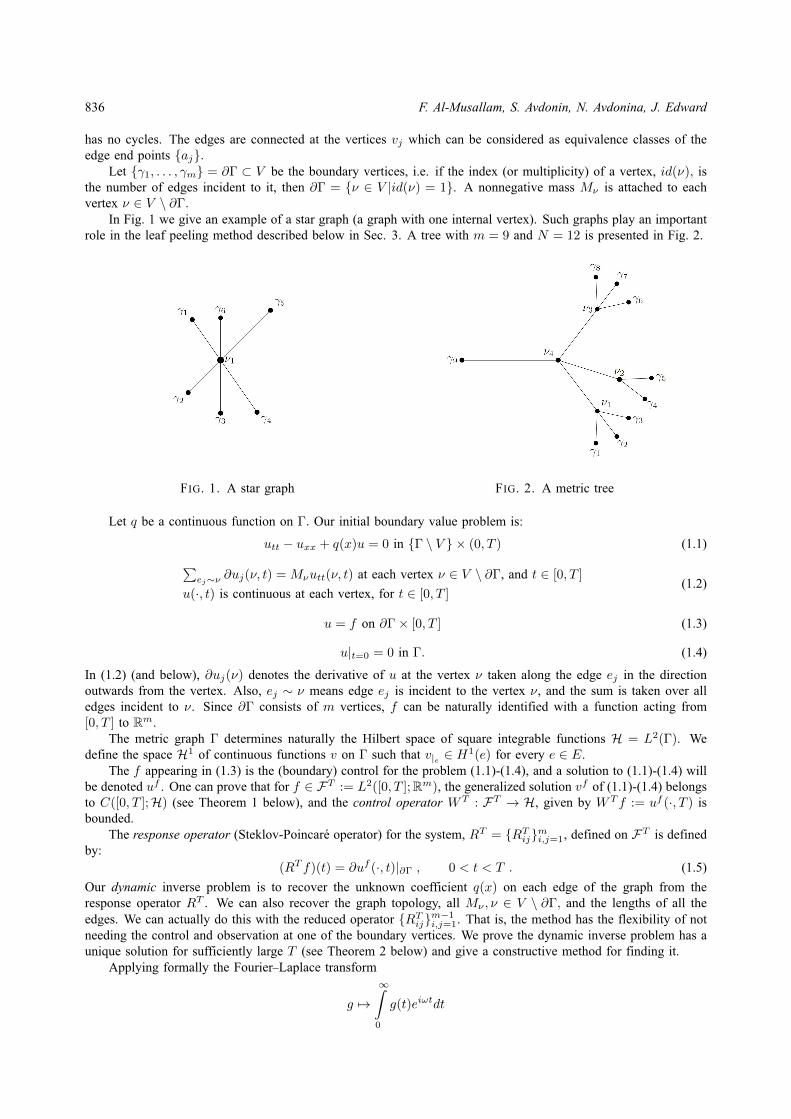
836 F. Al-Musallam, S. Avdonin, N. Avdonina, J. Edward
has no cycles. The edges are connected at the vertices vj which can be considered as equivalence classes of theedge end points aj.
Let γ1, . . . , γm = ∂Γ ⊂ V be the boundary vertices, i.e. if the index (or multiplicity) of a vertex, id(ν), isthe number of edges incident to it, then ∂Γ = ν ∈ V |id(ν) = 1. A nonnegative mass Mν is attached to eachvertex ν ∈ V \ ∂Γ.
In Fig. 1 we give an example of a star graph (a graph with one internal vertex). Such graphs play an importantrole in the leaf peeling method described below in Sec. 3. A tree with m = 9 and N = 12 is presented in Fig. 2.
FIG. 1. A star graph FIG. 2. A metric tree
Let q be a continuous function on Γ. Our initial boundary value problem is:
utt − uxx + q(x)u = 0 in Γ \ V × (0, T ) (1.1)∑ej∼ν ∂uj(ν, t) = Mνutt(ν, t) at each vertex ν ∈ V \ ∂Γ, and t ∈ [0, T ]
u(·, t) is continuous at each vertex, for t ∈ [0, T ](1.2)
u = f on ∂Γ× [0, T ] (1.3)
u|t=0 = 0 in Γ. (1.4)
In (1.2) (and below), ∂uj(ν) denotes the derivative of u at the vertex ν taken along the edge ej in the directionoutwards from the vertex. Also, ej ∼ ν means edge ej is incident to the vertex ν, and the sum is taken over alledges incident to ν. Since ∂Γ consists of m vertices, f can be naturally identified with a function acting from[0, T ] to Rm.
The metric graph Γ determines naturally the Hilbert space of square integrable functions H = L2(Γ). Wedefine the space H1 of continuous functions v on Γ such that v|e ∈ H1(e) for every e ∈ E.
The f appearing in (1.3) is the (boundary) control for the problem (1.1)-(1.4), and a solution to (1.1)-(1.4) willbe denoted uf . One can prove that for f ∈ FT := L2([0, T ];Rm), the generalized solution vf of (1.1)-(1.4) belongsto C([0, T ];H) (see Theorem 1 below), and the control operator WT : FT → H, given by WT f := uf (·, T ) isbounded.
The response operator (Steklov-Poincare operator) for the system, RT = RTijmi,j=1, defined on FT is definedby:
(RT f)(t) = ∂uf (·, t)|∂Γ , 0 < t < T . (1.5)
Our dynamic inverse problem is to recover the unknown coefficient q(x) on each edge of the graph from theresponse operator RT . We can also recover the graph topology, all Mν , ν ∈ V \ ∂Γ, and the lengths of all theedges. We can actually do this with the reduced operator RTij
m−1i,j=1. That is, the method has the flexibility of not
needing the control and observation at one of the boundary vertices. We prove the dynamic inverse problem has aunique solution for sufficiently large T (see Theorem 2 below) and give a constructive method for finding it.
Applying formally the Fourier–Laplace transform
g 7→∞∫
0
g(t)eiωtdt
Control and inverse problems for networks of vibrating strings with attached masses 837
to equations (1.1)–(1.3), we obtain the following boundary value problem depending on a complex parameterλ = ω2 :
−φxx(x, λ) + q(x)φ(x, λ) = λφ(x, λ) on Γ \ V , (1.6)∑ej∼ν ∂φj(ν, λ) = −λMνφ(ν, λ) at each vertex ν ∈ V \ ∂Γ,
φ(·, λ) is continuous at each vertex,(1.7)
The system of differential equations (1.6), (1.7) with zero Dirichlet boundary condition has only a trivial solutionfor λ /∈ R. Therefore, for any α ∈ Cm, this system of equations has a unique solution, φα(x, λ), satisfyingnon-zero boundary conditions:
φα(γj , λ) = αj , j = 1, 2, ...,m, α = col α1, . . . , αm, (1.8)
The m ×m matrix M(λ) defined by M(λ)α = ∂φα|∂Γ is called the Titchmarsh–Weyl matrix function, or theTW-function. The TW-function is also known as the (spectral) Dirichlet-to-Neumann map. The TW-functionM(λ)known for =λ > 0 will play the role of the spectral data for solving boundary inverse problems on graphs.
2. Main results
In the case of a string with loaded masses it was noticed [8, 9] that the wave transmitted through a mass ismore regular than the incoming wave. A similar effect also occurs for networks of strings. To formulate the result,we need the following definition. Among all paths from edge ei to the boundary vertex γj , let the degree, di, ofthe edge ei be the minimal (with respect to j) number of nonzero loaded masses on the path. For the followingtheorem we assume that q|ej ∈ Cdj (ej).
Theorem 1. Assume Mν > 0 for all ν. If f ∈ FT , then for any t ∈ [0, T ], uf (·, t) ∈ H and uf ∈ C([0, T ];H).Furthermore, for each ej ∈ E, uf |ej ∈ C([0, T ];Hdj (ej)).
The proof of the theorem is based on the analysis of the waves incoming to, transmitted through and reflectedfrom an inner vertex, taking into account the conditions (1.2). For the simplest graph of serially connected stringswith attached masses such a result was obtained in [8].
The next theorem describes the solution of the dynamic inverse problem.
Theorem 2. Let T∗ = 2 maxj 6=m distγj , γm. The operator RTijm−1i,j=1 known for T > T∗ uniquely determines
q on Γ, Mν : ν ∈ V \ ∂Γ, lj : j = 1, . . . , N and the graph topology. If the topology is known, all otherparameters can be found from the main diagonal RTii
m−1i=1 of the reduced response operator.
We also extend to our networks the leaf peeling method proposed in [5] (and generalized for strings withattached masses in [10]) and develop a constructive algorithm solving the inverse problem.
A spectral analog of Theorem 2 reads as follows.
Theorem 3. The reduced TW matrix function Mij(λ)m−1i,j=1 known for =λ > 0 uniquely determines q on Γ,
Mν : ν ∈ V \ ∂Γ, lj : j = 1, . . . , N and the graph topology. If the topology is known, all other parameterscan be found from the main diagonal Mii(λ)m−1
i=1 of the reduced TW matrix function.
3. Proof of Theorem 3
The response operator RT and TW-function M(λ) are connected with each other by the Fourier–Laplacetransform (see, e.g. [5]). Therefore, knowledge of M(λ) allows one to find RT for all T > 0, and knowledge ofRT for all T > 0 allows one to find M(λ).
In this section, we prove Theorem 3. We will give a brief description of an algorithm which allows us torecalculate the TW matrix function from the original graph to a smaller graph by “pruning” boundary edges.Ultimately, doing so allows us to reduce the original inverse problem on the graph to the inverse problem on asingle interval.
Our reduction algorithm combines both spectral and dynamical approaches, i.e. uses M(λ) and RT . As wementioned above, the TW matrix function determines the response operator for the system (1.1)-(1.4). Therefore,under the conditions of Theorem 3 the entries RTij , i, j = 1, . . . ,m− 1 are known for T > 0.
Step 1. Knowledge of RTjj for sufficiently large T allows one to recover the length of the edge e ∈ E incidentto γj , the potential q on e and the mass Mν , where ν ∈ V \ ∂Γ is an inner vertex to which e is incident. We canalso recover id(ν), the total number of edges incident to ν. The proof of these statements is based on the analysis
838 F. Al-Musallam, S. Avdonin, N. Avdonina, J. Edward
of the waves incoming to, transmitted through and reflected from vertex ν. Similar analysis was presented in [5]without the loaded masses; this was based on the boundary control method in inverse theory.
Step 2. We determine the boundary edges which have a common end point using the non-diagonal entries RTijof the response operator. Since the speed of wave propagation in the system (1.1)-(1.4) equals one, two boundaryedges, say, ei and ej , incident to the boundary edges γi and γj with the lengths li and lj have a common endpoint if and only if:
RTij =
0 for T < li + lj6= 0, for T > li + lj .
(3.1)
Definition of a sheaf. We consider a subgraph of Γ which is a star graph consisting of all edges incident to aninternal vertex v. This star graph is called a sheaf if all but one its edges are the boundary edges of Γ. It is knownthat any tree has at least two sheaves.
Step 3. Leaf peeling. We consider now a sheaf consisting, say, of several boundary edges e1, . . . , ep, p < m,incident to boundary vertices γ1, . . . , γp are connected at the vertex νs (see, e.g. vertices γ1, γ2, γ3, ν1 on Fig. 2).From Step 1, we know the potential on these edges, their lengths and the index of the vertex νs.
The index of the vertex νs is p+ 1 and there is exactly one internal edge incident to νs. We denote by M(λ)
the TW matrix function associated with the reduced graph Γ, i.e. the original graph Γ without the boundary edgese1, . . . , ep and vertices γ1, . . . , γp.
We denote by M0i(λ), Mi0(λ) and M00(λ) the entries of M(λ) related to the “new” boundary point νs0 ofthe graph Γ. The other entries of M(λ) are denoted by Mij , i, j = p + 1, . . . ,m. We demonstrate now how tofind the entries of M(λ).
First, we recalculate the entries M00(λ) and M0i(λ), i = p+ 1, . . . ,m− 1. we choose a boundary point, sayγ1, of the star-subgraph. Let φ(x, λ) be the solution to the problem (1.6), (1.7) subject to the boundary conditions:
φ(γ1, λ) = 1, φ(γj , λ) = 0, j = 2, . . . ,m− 1,m. (3.2)
We notice that on the boundary edge e1 the function φ solves the Cauchy problem:
−φ′′ + q(x)φ = λφ, x ∈ e1, (3.3)
φ(γ1, λ) = 1, φ′(γ1, λ) =M11(λ). (3.4)
On the other edges of the star subgraph it solves
−φ′′ + q(x)φ = λφ, x ∈ ei, i = 2, . . . , p, (3.5)
φ(γi, λ) = 0, φ′(γi, λ) =M1i(λ), i = 2, . . . , p. (3.6)
Since the potential on the edges e1, . . . , ep is known, we can solve the Cauchy problems (3.3), (3.4) and (3.5),(3.6) and use the matching conditions (1.7) at the internal vertex νs to recover the values φ(νs, λ) and φ′(νs, λ)on the “new” boundary edge at the “new” boundary point νs. Thus we obtain:
M00(λ) = φ′(νs,λ)φ(νs,λ) ,
M0i(λ) = M1i(λ)φ(νs,λ) , i = p+ 1, . . . ,m.
(3.7)
We recall that here =λ 6= 0, and so, φ(νs, λ) 6= 0. Otherwise, λ would be an eigenvalue of a selfadjoint operator.To find Mi0(λ) and Mij(λ) , i = p + 1, . . . ,m − 1 we fix γi (i > p) and consider the solution ψ(x, λ) to
(1.6), (1.7) with boundary conditions
ψ(γi, λ) = 1, ψ(γj , λ) = 0, j 6= i. (3.8)
The function ψ then solves the following Cauchy problems on the edges e1, . . . , ep:
−ψ′′ + q(x)ψ = λψ, x ∈ ej , j = 1, . . . , p, (3.9)
ψ(γj , λ) = 0, ψ′(γj , λ) =Mij(λ). (3.10)
Since we know the potential on the edges e1, . . . , ep, we can solve the Cauchy problems (3.9), (3.10) and use theconditions at the internal vertex νs to recover the values ψ(νs, λ) and ψ′(νs, λ) at the “new” boundary edge withthe “new” boundary point νs.
Now, we consider the following linear combination of the solutions φ and ψ:
ϕ(x, λ) = ψ(x, λ)− ψ(νs, λ)
φ(νs, λ)φ(x, λ) . (3.11)
Control and inverse problems for networks of vibrating strings with attached masses 839
It is easy to verify that on the subgraph Γ the function ϕ satisfies the boundary conditions:
ϕ(γi, λ) = 1, ϕ(γj , λ) = 0, j 6= i . (3.12)
Thus, from (3.11), we obtain that:
Mi0(λ) = ψ′(νs, λ)− ψ(νs, λ)M00(λ),
Mij(λ) =Mij(λ)− ψ(νs, λ)M0j(λ).(3.13)
To recover all elements of the reduced TW matrix function, we need to use this procedure for all i, j = p +1, . . . ,m− 1.
We conclude that the (reduced) TW-function for the graph Γ determines the (reduced) TW-function for thegraph Γ. The inverse problem is reduced to the inverse problem for a smaller graph. Since the graph Γ is finite,this procedure may be continued, but it ends after a finite number of steps.
The proofs of Theorems 1 and 2 for arbitrary tree will be presented in a forthcoming paper. The quantumgraph with the simplest topology — a network of serially connected strings — is considered in the next section.
4. Network of serially connected strings
We consider the wave equation on the interval [0, `] with N masses Mj > 0 attached at the points aj , j =1, . . . , N, where 0 = a0 < a1 < ... < aN < aN+1 = `. This is modeled by:
ρ(x)∂2u
∂t2− ∂2u
∂x2= 0, t ∈ (0, T ), x ∈ Ω := (0, a1) ∪ (a1, a2) ∪ . . . ∪ (aN , `),
u(a−j , t) = u(a+j , t), Mj utt(aj , t) = ux(a+
j , t)− ux(a−j , t),
u(x, 0) = ut(x, 0) = 0,
u(0, t) = f(t), f ∈ FT := L2(0, T ), u(`, t) = 0.
Here ρ is a positive function on [0, `] and ρ|[aj ,aj+1] ∈ Cj+2[aj , aj+1], j = 0, . . . , N .We show that the wave transmitted through a mass is more regular than the incoming wave. We define the
spaces W, WT :
W =φ ∈ L2(0, a1)×H1(a1, a2)× ...HN (aN , `) :
φ(a−j ) = φ(a+j ), φ′(a−j ) = φ′(a+
j )−Mj φ′′(a+
j )/ρ(a+j ), φ(`) = 0
,
WT = φ ∈W : φ(x) = 0 for x ≥ X(T ) ,where
T =
X(T )∫0
√ρ(x) dx , L =
l∫0
√ρ(x) dx .
The following result on the regularity of the solution of the initial boundary value problem stated above andon the controllability of this dynamical system has been proved in [8].
Theorem 4. Suppose T ≤ L :=l∫
0
√ρ(x) dx. For any f ∈ FT , uf ∈ C(0, T ;WT ) and for any φ ∈ WT , there
exists a unique f ∈WT such that uf (x, T ) = φ(x). Furthermore,
‖uf (·, T )‖W ‖f‖FT .
For T > L,
uf (·, T ) : f ∈ L2(0, T ) = W.
Our dynamical inverse problem is to recover unknown parameters of the system from the response operator
RT : FT 7→ FT , Dom(RT ) = f ∈ H1(0, T ), f(0) = 0,
(RT f)(t) = ufx(0, t), t ∈ (0, T ).
The main result is this section is:
Theorem 5. Let T > 2L. Given RT , one can find ρ(x), l, aj , and Mj , j = 1, . . . , N.
840 F. Al-Musallam, S. Avdonin, N. Avdonina, J. Edward
We prove this theorem in several steps. First, we consider the spectral boundary value problem correspondingour dynamical system:
−ϕ′′(x, λ) = λ2ρ(x)ϕ(x, λ), x ∈ Ω,
ϕ(0, λ) = ϕ(`, λ) = 0, ϕ(a−j , λ) = ϕ(a+j , λ),
−Mj λ2ϕ(aj , λ) = ϕ′(a+
j , λ)− ϕ′(a−j , λ) ∀j.The eigenvalues λ2
n of this problem are simple and the eigenfunctions ϕn form the orthonormal basis in the spaceH := L2
ρ(0, l)⊕RN with the inner product:
〈φ, ψ〉H =
l∫0
φ(x)ψ(x)ρ(x)dx+
N∑j=1
Mjφ(aj)ψ(aj) .
We setHT = φ ∈ H : φ(x) = 0 for x ≥ X(T ) .
The connecting operator is defined as:
CT : FT 7→ FT , (CT f, g)FT :=⟨uf (·, T ), ug(·, T )
⟩H .
The connecting operator can be written in the form CT = (UT )∗(UT ) where
UT : FT 7→WT , UT f = uf (·, T ).
The exact controllability (see Theorem 4) implies that CT is bounded and boundedly invertible.Our second step is:
Theorem 6. Operator CT can be explicitly expressed through the response operator on the double interval:CT = − 1
2 (ST )∗I2TR2TST , where:
(ST f)(t) =
f(t) if t ∈ [0, T ],
−f(2T − t) if t ∈ (T, 2T ],(I2T f)(t) =
t∫0
f(s)ds.
Sketch of the proof of Theorem 6. Set w(s, t) :=⟨uf (·, s), ug(·, t)
⟩H .
We notice that (CT f, g)FT = w(T, T and
wtt(s, t)− wss(s, t) =
l∫0
[uf (x, s)ugtt(x, t)− ufss(x, s)ug(x, t)]ρ(x)dx
+∑j
Mj [uf (aj , s)u
gtt(aj , t)− ufss(aj , s)ug(aj , t)] = (using ρutt = uxx)
=[uf (x, s)ugx(x, t)− ufx(x, s)ug(x, t)
]lx=0
= (Rf)(s)g(t)− f(s)(Rg)(t).
We use w(s, 0) = wt(s, 0) = w(0, t) = 0 to find w(T, T ) by D’Alembert’s formula.The next step is the construction of special bases in spaces FT and HT . Let T ≤ L and fn, n ∈ N , be
a basis in FT such that:
f ∈ C2[0, T ], f(0) = f ′(0) = 0,(CT fk, fn
)FT = δkn.
Due to controllability, ufn(·, T ) is an orthonormal basis in HT .
Next, we introduce two functions: φ0(x) = 1, φ1(x) = x, x ∈ [0, l] and let φ0T and φ1
T be their restrictionsto the interval [0, X(t)].
Theorem 7. The coefficients in the series representations of the functions φ0T , φ
1T with respect to the basis
ufj (·, T ) have the form
c0n := 〈φ0, ufn(·, T )〉H = −T∫
0
(T − t)(RT fn)(t) dt ,
c1n := 〈φ1, ufn(·, T )〉H =
T∫0
(T − t) fn(t) dt .
Control and inverse problems for networks of vibrating strings with attached masses 841
Sketch of the proof of Theorem 7. By the definition of the connection operator, we have:
〈φ0, ufn(·, T )〉H =
l∫0
ufn(x, T )ρ(x)dx+∑j
Mj ufn(aj , T )
=
T∫0
(T − t)
X(T )∫0
ufntt (x, t)ρ(x)dx+∑j
Mj ufntt (aj , t)
dt=
T∫0
(T − t)
X(T )∫0
ufnxx(x, t)dx+∑j
Mj ufntt (aj , t)
dt= −
T∫0
(T − t)ufnx (0, t) dt = −T∫
0
(T − t)(RT fn)(t) dt.
This proves the first statement of Theorem 7. The second one can be proved in a similar way.Now, we are ready to complete the solution of the dynamical inverse problem. We introduce two functions:
µ(T ) =
X(T )∫0
ρ(x)dx+∑
j: aj<X(T )
Mj ,
ν(T ) =
X(T )∫0
xρ(x)dx+∑
j: aj<X(T )
Mj aj .
They can be found using the theorem:
µ(T ) = 〈φ0T , φ
0T 〉H =
∑n
|c0n|2, ν(T ) = 〈φ0T , φ
1T 〉H =
∑n
c0n c1n .
Separating the singular and regular (integral) parts, we find Mj and aj from the singular parts. From the regularparts, we have:
µr(T ) = ρ(X(T )) X(T ), νr(T ) = X(T )ρ(X(T )) X(T ) .
From these relations, we find X(T ) and, finally, ρ(x).
Acknowledgments
The research of S. Avdonin was supported in part by the National Science Foundation, grant DMS 1411564and by the Ministry of Education and Science of Republic of Kazakhstan under the grant No. 4290/GF4.
References
[1] Gerasimenko N.I., Pavlov B.S. Scattering problems on noncompact graphs, Teoret. Mat. Fiz., 1988, 74, P. 345–359. Eng. transl., Theoret.and Math. Phys., 1988, 74, P. 230–240.
[2] Gerasimenko N.I. Inverse scattering problem on a noncompact graph. Teoret. Mat. Fiz., 1988, 75, P. 187–200. Translation in Theoret. andMath. Phys., 1988, 75, P. 460–470.
[3] Berkolaiko G., Kuchment P. Introduction to Quantum Graphs (Mathematical Surveys and Monographs vol 186). Providence, RI: AmericanMathematical Society, 2013.
[4] Avdonin S. Control problems on quantum graphs. Analysis on Graphs and Its Applications, Proceedings of Symposia in Pure Mathematics,AMS, 2008, 77, P. 507–521.
[5] Avdonin S., Kurasov P. Inverse problems for quantum trees. Inverse Problems and Imaging, 2008, 2 (1), P. 1–21.[6] Avdonin S., Bell J. Determining a distributed conductance parameter for a neuronal cable model defined on a tree graph. Journal of
Inverse Problems and Imaging, 2015, 9 (3), P. 645–659.[7] Avdonin S., Choque Rivero A., Leugering G., and Mikhaylov V. On the inverse problem of the two velocity tree-like graph. Zeit. Angew.
Math. Mech., 2015, 1–11. DOI 10.1002 zamm.201400126.[8] Avdonin S. and Edward J. Inverse problems for networks of vibrating strings with attached masses. SIAM Journal of Control and
Optimization, submitted.[9] Hansen S. and Zuazua E. Exact controllability and stabilization of a vibrating string with an interior point mass. SIAM J. Control Optim.,
1995, 33 (5), P. 1357–1391.[10] Avdonin S., Avdonina N. and Edward J. Boundary inverse problems for networks of vibrating strings with attached masses. Proceedings
of Dynamic Systems and Applications, 2016, 7, P. 41–44.
NANOSYSTEMS: PHYSICS, CHEMISTRY, MATHEMATICS, 2016, 7 (5), P. 842–853
Dynamical inverse problem for the discrete Schrodinger operator
A. S. Mikhaylov1,2, V. S. Mikhaylov1,2
1St. Petersburg Department of V. A. Steklov Institute of Mathematics of the Russian Academy of Sciences,7, Fontanka, 191023, St. Petersburg, Russia
2St. Petersburg State University, 7/9 Universitetskaya nab., 199034, St. Petersburg, Russia
[email protected], [email protected]
DOI 10.17586/2220-8054-2016-7-5-842-853
We consider the inverse problem for the dynamical system with discrete Schrodinger operator and discrete time. As inverse data, we take
a response operator, the natural analog of the dynamical Dirichlet-to-Neumann map. We derive two types of equations of inverse problem
and answer a question on the characterization of the inverse data, i.e. we describe the set of operators, which are response operators of the
dynamical system governed by the discrete Schrodinger operator.
Keywords: inverse problem, discrete Schrodinger operator, Boundary Control method, characterization of inverse data.
Received: 19 July 2016
Revised: 21 August 2016
Dedicated to the memory of B. S. Pavlov
1. Introduction
The theory of dynamical inverse problems is a wide area of modern mathematics, by now for all or almostall linear nonstationary equations of mathematical physics there exist an inverse theory more or less developed.Theories mostly covers the case of continuous problems, at the same time just a few attention is paid to discreteones. The primary goal of the paper is to improve this situation.
Let N be the set of positive natural numbers, N0 = N ∪ 0. We fix the infinite sequence of real num-bers (b1, b2, . . .), which we call the potential and consider the dynamical system with discrete time which is anatural analog of dynamical systems governed by the wave equation with potential on a semi-axis:
un,t+1 + un,t−1 − un+1,t − un−1,t + bnun,t = 0, n, t ∈ N0,
un,−1 = un,0 = 0, n ∈ N,u0,t = ft, t ∈ N0.
(1.1)
By analogy with continuous problems [1], we treat the real sequence f = (f0, f1, . . .) as a boundary control. Thesolution to (1.1) we denote by ufn,t.
Having fixed τ ∈ N, with (1.1) we associate the response operators, which maps the control f = (f0, . . . fτ−1)
to uf1,t:
(Rτf)t := uf1,t, t = 1, . . . , τ. (1.2)
The inverse problem we will be dealing with is to recover from Rτ (part of the) potential (b1, b2, . . . , bn) for somen. This problems is a natural discrete analog of the inverse problem for the wave equation where the inverse datais the dynamical Dirichlet-to-Neumann map, see [1].
We will be using the Boundary Control method [1] which was initially developed to treat multidimensionaldynamical inverse problems, but since then was applied to multi- and one- dimensional inverse dynamical, spectraland scattering problems, problems of signal processing and identification problems [2, 3].
In the second section, we study the forward problem: for (1.1) we prove the analog of d’Alembert integralrepresentation formula. Prescribing the Dirichlet condition at n = N+1, we consider the second dynamical systemwith boundary control at n = 0 (which will be an analog of the problem on the finite interval) and develop thesolution of this system in Fourier series. We analyze the dependence of two solutions on the potential, which leadus to the natural set up of the inverse problem. In the third section, we introduce and prove the representationformulae for the main operators of the BC method: response operator, control and connecting operators. In thefourth section, we derive two types of equations for the inverse problem and give a characterization of the inversedata. In the last section, we highlight the connections between the different types of inverse data.
The case of the Jacobi matrices of general type as well as the studying of the inverse spectral problem, i.e.recovering the semi-infinite matrix from the spectral measure, will be the subject of forthcoming publications.
Dynamical inverse problem for the discrete Schrodinger operator 843
2. Forward problems
We fix some positive integer T . By FT we denote the space of controls: FT := RT , f ∈ FT , f = (f0, . . . , fT−1).First, we derive the representation formulas for the solution to (1.1) which could be considered as analogs of
known formulas for the wave equation [4].
Lemma 1. The solution to (1.1) admits the representation:
un,t = ft−n +
t−1∑s=n
wn,sft−s−1, n, t ∈ N0. (2.1)
where wn,s satisfies the Goursat problem:wn,t+1 + wn,t−1 − wn+1,t − wn−1,t + bnwn,t = 0, n, s ∈ N0, s > n,
wn,n = −n∑k=1
bk, n ∈ N,
w0,t = 0, t ∈ N0.
(2.2)
Proof. We assume that ufn,t has a form (2.1) with unknown wn,s and plug it to equation in (1.1):
0 = bnft−n +t−1∑s=n
bnwn,sft−s−1 +
t∑s=n
wn,sft−s +
t−2∑s=n
wn,sft−s−2 −t−1∑
s=n+1
wn,sft−s−1 −t−1∑
s=n−1wn−1,sft−s−1.
Changing the order of summation, we get:
0 = bnft−n + wn+1,nft−n−1 − wn−1,n−1ft−n +
t−1∑s=n
ft−s−1 (bnwn,s − wn+1,s − wn−1,s)
+
t−1∑s=n−1
wn,s+1ft−s−1 +
t−1∑s=n+1
wn,s−1ft−s−1 = ft−n−1(wn+1,n − wn,n−1) + bnft−n
+
t−1∑s=n
ft−s−1 (wn,s+1 + wn.s−1 − wn+1,s − wn−1,s + bnwn,s) + ft−n(wn,n − wn−1,n−1).
Counting that wn,s = 0 when n > s and arbitrariness of f ∈ FT , we arrive at (2.1).
We fix N ∈ N. Along with (1.1) we consider the analog of the wave equation with the potential on theinterval: we assume that (bn) is finite: n = 1, . . . , N and impose the Dirichlet condition at n = N + 1. Then fora control f = (f0, f1, . . .) we consider:
vn,t+1 + vn,t−1 − vn+1,t − vn−1,t + bnvn,t = 0, t ∈ N0, n ∈ 0, . . . , N + 1
vn,−1 = vn,0 = 0, n = 1, 2, . . . , N + 1
v0,t = ft, vN+1,t = 0, t ∈ N0.
(2.3)
We denote the solution to (2.3) by vf .Let φn(λ) be the solution to:
φi+1 + φi−1 − bnφi = λφi,
φ0 = 0, φ1 = 1.(2.4)
We introduce the Hamiltonian:
HN :=
−b1 1 0 . . . 0
1 −b2 1 . . . 0
· · · · ·0 . . . 0 1 −bN
Let ϕk, λkNk=1 be eigenvectors chosen such that ϕk1 = 1 and eigenvalues of HN . Introduce the numbers ρk by:
(ϕk, ϕl) = δklρk, (2.5)
where (·, ·)– is a scalar product in RN .
844 A. S. Mikhaylov, V. S. Mikhaylov
Definition 1. The setλk, ρkNk=1 (2.6)
is called the spectral data.
On introducing vectors φn ∈ RN by the rule φni := φi(λn), n, i = 1, . . . , N, we have
Proposition 1. The solutions of φN+1(λ) = 0 are λn, n = 1, . . . , N ; and φni = ϕni , n, i = 1, . . . , N.
Proof. Take eigenvector ϕn corresponding to eigenvalue λn and compare it with φn. By the definition of ϕn andcondition in (2.4): ϕn1 = φn1 = 1. On the other hand, comparing the first line in the equation on eigenvaluesHNϕ
n = λnϕn and (2.4) for i = 1 we have:
−ϕn1 b1 + ϕn2 = λnϕn1 ,
φn2 − b1φn1 = λnφn1 ,
which implies ϕn2 = φn2 , for k < N comparing k−th line in HNϕn = λnϕn and (2.4) for i = k, we arrive at
ϕnk+1 = φnk+1. And for k = N :
−ϕnNbN + ϕnN−1 = λnϕnN ,
φnN+1 + φnN−1 − bNφnN = λnφnN ,
which holds if and only if φnN+1(λn) = 0.
We take y ∈ RN , y = (y1, . . . , yN ), for each n we multiply the equation in (2.3) by yn, sum up and evaluatethe following expression, changing the order of summation:
0 =
N∑n=1
(vn,t+1yn + vn,t−1yn − vn+1,tyn − vn−1,tyn + bnvn,tyn) =
N∑n=1
(vn,t+1yn + vn,t−1yn − vn,t(yn−1 + yn+1) + bnvn,tyn)− vN+1,tyN − v0,ty1 + v1,ty0 + vN,tyN+1. (2.7)
Now, we choose y = ϕl, l = 1 . . . , N . On counting that ϕl0 = ϕlN+1 = 0, ϕl1 = 1, v0,t = ft, vN+1,t = 0 weevaluate (2.7) arriving at:
0 =
N∑n=1
(vn,t+1ϕ
ln + vn,t−1ϕ
ln − vn,t
(ϕln−1 + ϕln+1 − bnϕln
))− ft = 0. (2.8)
Definition 2. For a, b ∈ l∞, we define the convolution c = a ∗ b ∈ l∞ by the formula:
ct =
t∑s=0
asbt−s, t ∈ N.
We assume that the solution to (2.3) has the form:
vfn,t =
N∑k=1
cktϕkn, n = 1, . . . , N
ft, n = 0.
(2.9)
Proposition 2. The coefficients ck admits the representation:
ck =1
ρkT (λk) ∗ f, (2.10)
where T (2λ) = (T1(2λ), T2(2λ), T3(2λ), . . .) are Chebyshev polynomials of the second kind.
Proof. We plug (2.9) into (2.8) and evaluate, counting that ϕln−1 + ϕln+1 − bnϕln = λlϕln:
N∑n=1
(vn,t+1 + vn,t−1 − λlvn,t)ϕln = ft,
N∑n=1
N∑k=1
(ckt+1ϕ
kn + ckt−1ϕ
kn − λlcktϕkn
)ϕln = ft.
Dynamical inverse problem for the discrete Schrodinger operator 845
Changing the order of summation and using (2.5), we finally arrive at the following equation on ckt , k = 1, . . . , N : ckt+1 + ckt−1 − λkckt =1
ρkft,
ck−1 = ck0 = 0.(2.11)
We assume that the solution to (2.11) has the form: ck =1
ρkT ∗ f, or
ckt =1
ρk
t∑l=0
Tlft−l. (2.12)
Plugging it into (2.11), we get:
1
ρk
(t+1∑l=0
flTt+1−l +
t−1∑l=0
flTt−1−l − λkt∑l=0
flTt−l
)=
1
ρkft,
t∑l=0
fl (Tt+1−l + Tt−1−l − λkTt−l) + ftT1 − ft−1T0 = ft.
We see that (2.12) holds if T solves: Tt+1 + Tt−1 − λkTt = 0,
T0 = 0, T1 = 1.
Thus Tk(2λ) are Chebyshev polynomials of the second kind.
3. Operators of the the BC method
As inverse data for (1.1), we use the analog of the dynamical response operator (dynamical Dirichlet-to-Neumann map) [1].
Definition 3. For (1.1), the response operator RT : FT 7→ RT is defined by the rule(RT f
)t= uf1,t, t = 1, . . . , T.
Introduce the notation: the response vector is the convolution kernel of the response operator, r = (r0, r1, . . . , rT−1) =(1, w1,1, w1,2, . . . w1,T−1). Then, in accordance with (2.1):(
RT f)t= uf1,t = ft−1 +
t−1∑s=1
w1,sft−1−s, t = 1, . . . , T ; (3.1)(RT f
)= r ∗ f·−1, where r0 = 1.
For system (2.3), we introduce the response operator by:
Definition 4. For the system in (2.3) the response operator RTi : FT 7→ RT is defined by the rule:(RTi f
)t= vf1,t, t = 1, . . . , T. (3.2)
The corresponding response vector we denote by (ri1, ri2, . . .). More information on this operator and on the
inverse spectral problem one can find in the last section.We introduce the inner space of dynamical system (1.1) HT := RT , h ∈ HT , h = (h1, . . . , hT ). For (1.1)
The control operator WT : FT 7→ HT is defined by the rule:
WT f := ufn,T , n = 1, . . . , T.
Directly from (2.1), we deduce that:(WT f
)n= ufn,T = fT−n +
T−1∑s=n
wn,sfT−s−1, n = 1, . . . , T. (3.3)
The following statement imply the controllability of the dynamical system (1.1).
846 A. S. Mikhaylov, V. S. Mikhaylov
Theorem 1. The operator WT is an isomorphism between FT and HT .
Proof. We fix some a ∈ HT and look for a control f ∈ FT such that WT f = a. To this aim we write down theoperator as:
WT f =
u1,Tu2,T·
uk,T·
uT,T
=
1 w1,1 w1,2 . . . . . . w1,T−1
0 1 w2,2 . . . . . . w2,T−1
· · · · · ·0 . . . 1 wk,k . . . wk,T−1· · · · · ·0 0 0 0 . . . 1
fT−1fT−2·
fT−k−1·f0
(3.4)
We introduce the notations:
JT : FT 7→ FT , (JT f)n = fT−1−n, n = 0, . . . , T − 1,
K ∈ RT×T , kij = 0, i > j, kii = 1, kij = wij−1, i < j.
Then, WT = (I +K) JT . Obviously, this operator is invertible, which proves the statement of the theorem.
For the system (2.3) the control operator WTi : FT 7→ HN is defined by the rule:
WTi f := vfn,T , n = 1, . . . , N.
The representation for this operator immediately follows from (2.9), (2.10).For the system (1.1) we introduce the connecting operator CT : FT 7→ FT by the quadratic form: for arbitrary
f, g ∈ FT we define (CT f, g
)FT =
(uf·,T , u
g·,T
)HT
=(WT f,WT g
)HT . (3.5)
We observe that CT =(WT
)∗WT , so CT is an isomorphism in FT . The fact that CT can be expressed in terms
of response R2T is crucial in BC-method.
Theorem 2. Connecting operator admits the representation in terms of inverse data:
CT = CTij , CTij =
T−max i,j∑k=0
r|i−j|+2k, r0 = 1. (3.6)
CT =
1 + r2 + . . .+ r2T−2 r1 + r3 + . . .+ r2T−3 . . . rT + rT−2 rT−1r1 + r3 + . . .+ r2T−3 1 + r2 + . . .+ r2T−4 . . . . . . rT−2
· · · · ·rT−3 + rT−1 + rT+1 . . . 1 + r2 + r4 r1 + r3 r2
rT + rT−2 . . . r1 + r3 1 + r2 r1rT−1 rT−2 . . . r1 1
Proof. For fixed f, g ∈ FT , we introduce the Blagoveshchensky function by:
ψn,t :=(uf·,n, u
g·,t)HT =
T∑k=1
ufk,nugk,t.
Then, we show that ψn,t satisfies some difference equation. Indeed, we can evaluate:
ψn,t+1 + ψn,t−1 − ψn+1,t − ψn−1,t =T∑k=1
ufk,n
(ugk,t+1 + ugk,t−1
)−
T∑k=1
(ufk,n+1 + ufk,n−1
)ugk,t =
T∑k=1
ufk,n
(ugk+1,t + ugk−1,t
)−
T∑k=1
(ufk+1,n + ufk−1,n
)ugk,t =
T∑k=1
ugk,t
(ufk+1,n + ufk−1,n
)+ ug0,tu
f1,n − u
f0,nu
g1,t + ugT+1,tu
fT,n − u
fT+1,nu
gT,t −
T∑k=1
ugk,t
(ufk+1,n + ufk−1,n
)=
gt(Rf)n − fn(Rg)t.
Dynamical inverse problem for the discrete Schrodinger operator 847
So, we arrive at the following boundary problem for ψn,t:ψn,t+1 + ψn,t−1 − ψn+1,t − ψn−1,t = hn,t, n, t ∈ N0,
ψ0,t = 0, ψn,0 = 0,(3.7)
hn,t = gt(Rf)n − fn(Rg)t.We introduce the set:
K(n, t) :=(n, t) ∪ (n− 1, t− 1), (n+ 1, t− 1) ∪ (n− 2, t− 2), (n, t− 2), (n+ 2, t− 2) ∪ . . .
∪(n− t, 0), (n− t+ 2, 0), . . . , (n+ t− 2, 0), (n+ t, 0)=
t⋃τ=0
τ⋃k=0
(n− τ + 2k, t− τ) .
The solution to (3.7) is given by:
ψn,t =∑
k,τ∈K(n,t−1)
h(k, τ).
We observe that ψT,T =(CT f, g
), so: (
CT f, g)=
∑k,τ∈K(T,T−1)
h(k, τ). (3.8)
Notice that in the r.h.s. of (3.8) the argument k runs from 1 to 2T − 1. We extend f ∈ FT , f = (f0, . . . , fT−1) tof ∈ F2T by:
fT = 0, fT+k = −fT−k, k = 1, 2, . . . , T − 1.
Due to this odd extension,∑
k,τ∈K(T,T−1)
fk(RT g)τ = 0, so (3.8) gives:
(CT f, g
)=
∑k,τ∈K(T,T−1)
gτ(R2T f
)k= g0
[(R2T f
)1+(R2T f
)3+ . . .+
(R2T f
)2T−1
]+ g1
[(R2T f
)2+(R2T f
)4+ . . .+
(R2T f
)2T−2
]+ . . .+ gT−1
(R2T f
)T.
Finally, we infer that:
CT f =((R2T f
)1+ . . .+
(R2T f
)2T−1 ,
(R2T f
)2+ . . .+
(R2T f
)2T−2 , . . . ,
(R2T f
)T
)from where the statement of the theorem follows.
One can observe that CTij satisfies the difference boundary problem.
Corollary 1. The kernel of CT satisfy:CTi,j+1 + CTi,j−1 − CTi+1,j − CTi−1,j = 0,
CTi,T = rT−i, CTT,j = rT−j , r0 = 1.
For the system (2.3) the connecting operator CTi : FT 7→ FT is introduced in the similar way: for arbitraryf, g ∈ FT we define: (
CTi f, g)FT =
(vf·,T , v
g·,T
)HN
=(WTi f,W
Ti g)HN . (3.9)
More information on CTi one can find in the final section.
4. Inverse problem
The dependence of the solution (1.1) uf on the potential (b1, b2, . . .) resembles one of the wave equation withthe potential: take some M ∈ N. From the very equation, one can see that the term ufn,t with smallest n, t,which depends on bM is ufM,M+1. Thus, uf1,t becomes dependent upon bM starting from t = 2M . This is ananalog of the finite wave propagation speed effect in the wave equation. Consider (2.3) with N =M . We see thatthe solution to (2.3) vf1,t does not ‘feel’ the boundary condition at n = M + 1: uf1,t = vf1,t for t = 1, . . . , 2M . Or
in other words, that means that R2M = R2Mi . This leads to the following natural set up of the inverse problem:
By the given operator R2M to recover the (part) of the potential (b1, . . . , bM ). In what follows, we will be dealingwith the IP for the system (1.1), only in the last section we comment on the system (2.3).
848 A. S. Mikhaylov, V. S. Mikhaylov
4.1. Krein equations
Let α, β ∈ R and y be solution to: yk+1 + yk−1 − bkyk = 0,
y0 = α, y1 = β.(4.1)
We set up the following control problem: to find a control fT ∈ FT such that:(WT fT
)k= yk, k = 1, . . . , T. (4.2)
Due to Theorem 1, this problem has unique solution. Let κT be a solution toκTt+1 + κTt−1 = 0, t = 0, . . . , T,
κTT = 0, κTT−1 = 1.(4.3)
We show that the control fT satisfies the Krein equation:
Theorem 3. The control fT , defined by (4.2) satisfies the following equation in FT :
CT fT = βκT − α(RT)∗ κT . (4.4)
Proof. Let us take fT solving (4.2). We observe that for any fixed g ∈ FT :
ugk,T =
T−1∑t=1
(ugk,t+1 + ugk,t−1
)κTt . (4.5)
Indeed, changing the order of summation in the r.h.s. of (4.5), we get:
T−1∑t=1
(ugk,t+1 + ugk,t−1
)κTt =
T−1∑t=1
(κTt+1 + κTt−1
)ugk,t + ugk,0κ
T1 − u
gk,Tκ
TT−1.
which gives (4.5) due to (4.3). Using this observation, we can evaluate:
(CT fT , g
)=
T∑k=1
ykugk,T =
T∑k=1
T−1∑t=0
(ugk,t+1 + ugk,t−1
)κTt yk
=
T−1∑t=0
κTt
(T∑k=1
(ugk+1,tyk + ugk−1,tyk − bku
gk,tyk
))
=
T−1∑t=0
κTt
(T∑k=1
(ugk,t(yk+1 + yk−1 − bkyk
)+ ug0,ty1 + ugT+1,tyT − u
g1,ty0 − u
gT,tyT+1
)
=
T−1∑t=0
κTt(βgt − α
(RT g
)t
)=(κT , βg − α
(RT g
))=(βκT − α
((RT)∗ κT) , g) .
From where (4.4) follows.
Having found fτ for τ = 1, . . . , T , we can recover the potential bn, n = 1, . . . , T − 1. Indeed: by theconstructions of fτ we have (W τfτ )τ = yτ , on the other hand, from (3.3) we can infer that (W τfτ )τ = fτ0 , thusy (4.1) can be recovered by:
yτ = fτ0 , τ = 1, . . . , T. (4.6)
And the potential can be found by:
bn =yn+1 + yn−1
yn, n = 1, . . . , T − 1. (4.7)
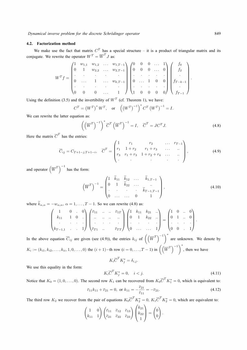
Dynamical inverse problem for the discrete Schrodinger operator 849
4.2. Factorization method
We make use the fact that matrix CT has a special structure – it is a product of triangular matrix and its
conjugate. We rewrite the operator WT =WTJ as:
WT f =
1 w1,1 w1,2 . . . w1,T−1
0 1 w2,2 . . . w2,T−1
· · · · ·0 . . . 1 . . . wk,T−1· · · · ·0 0 0 . . . 1
0 0 0 . . . 1
0 0 0 . . . 0
· · · · ·0 . . . 1 0 0
· · · · ·1 0 0 0 0
f0f2·
fT−k−1·
fT−1
.
Using the definition (3.5) and the invertibility of WT (cf. Theorem 1), we have:
CT =(WT
)∗WT , or
((WT
)−1)∗CT(WT
)−1= I.
We can rewrite the latter equation as:((W
T)−1)∗
CT(W
T)−1
= I, CT= JCTJ. (4.8)
Here the matrix CT
has the entries:
Cij = CT+1−j,T+1−i, CT=
1 r1 r2 . . . rT−1r1 1 + r2 r1 + r3 . . . ..
r3 r1 + r3 1 + r2 + r4 . . . ..
· · · · ·
, (4.9)
and operator(W
T)−1
has the form:
(W
T)−1
=
1 k11 k12 . . . k1,T−1
0 1 k22 . . . ..
· · · · kT−1,T−10 . . . . . . 0 1
, (4.10)
where kα,α = −wα,α, α = 1, . . . , T − 1. So we can rewrite (4.8) as:1 0 . 0
k11 1 0 .
· · · ·kT−1,1 . . 1
c11 .. .. c1T.. .. .. ..
· · · ·cT1 .. cTT
1 k11 k21 ..
0 1 k22 ..
· · · ·0 . . . . . . 1
=
1 0 .. 0
0 1 .. 0
· · · ·0 0 . 1
.
In the above equation Cij are given (see (4.9)), the entries kij of
((W
T)−1)∗
are unknown. We denote by
Ki := (ki1, ki2, . . . , kii, 1, 0, . . . , 0) the (i+ 1)−th row (i = 0, . . . , T − 1) in
((W
T)−1)∗
, then we have
KiCTK∗j = δi,j .
We use this equality in the form:
KiCTK∗j = 0, i < j. (4.11)
Notice that K0 = (1, 0, . . . , 0). The second row K1 can be recovered from K0CTK∗1 = 0, which is equivalent to:
c11k11 + c21 = 0, or k11 = −c21c11
= −c21. (4.12)
The third row K2 we recover from the pair of equations K0CTK∗2 = 0, K1C
TK∗2 = 0, which are equivalent to:(
1 0
k11 1
)(c11 c12 c13c21 c22 c23
)k21k221
=
(0
0
).
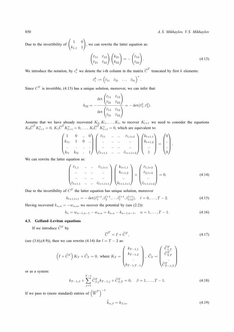
850 A. S. Mikhaylov, V. S. Mikhaylov
Due to the invertibility of
(1 0
k1,1 1
), we can rewrite the latter equation as:
(c11 c12c21 c22
)(k21k22
)= −
(c13c23
). (4.13)
We introduce the notation, by cki we denote the i-th column in the matrix CT
truncated by first k elements:
cki :=(c1i c2i . . . cki
)∗.
Since CT is invertible, (4.13) has a unique solution, moreover, we can infer that:
k22 = −det
(c11 c13c21 c23
)
det
(c11 c12c21 c22
) = −det(c21, c23).
Assume that we have already recovered K0,K1, . . . ,Kl, to recover Kl+1 we need to consider the equations
K0CTK∗l+1 = 0, K1C
TK∗l+1 = 0, . . . , KlC
TK∗l+1 = 0, which are equivalent to:
1 0 .. 0
k11 1 0 ..
. . . .
kl1 kl2 . 1
c11 .. .. c1,l+2
.. .. .. ..
.. .. .. ..
cl+1,1 .. .. cl+1,l+2
kl+1,1
kl+1,2
..
1
=
0
..
..
0
.
We can rewrite the latter equation as:c1,1 .. .. c1,l+1
.. .. .. ..
.. .. .. ..
cl+1,1 .. .. cl+1,l+1
kl+1,1
kl+1,2
..
kl+1,l+1
+
c1,l+2
c2,l+2
..
cl+1,l+2
= 0. (4.14)
Due to the invertibility of CT the latter equation has unique solution, moreover
kl+1,l+1 = −det(cl+11 , cl+1
2 , . . . cl+1l , cl+1
l+2), l = 0, . . . , T − 2. (4.15)
Having recovered kα,α = −wα,α, we recover the potential by (see (2.2)):
bn = wn−1,n−1 − wn,n = kn,n − kn−1,n−1, n = 1, . . . , T − 1. (4.16)
4.3. Gelfand–Levitan equations
If we introduce CT by
CT= I + CT , (4.17)
(see (3.6),(4.9)), then we can rewrite (4.14) for l = T − 2 as:
(I + CT
)KT + CT = 0, where KT =
kT−1,1kT−1,2.
kT−1,T−1
, CT =
CT1,TCT2,T.
CTT−1,T
or as a system:
kT−1,β +
T−1∑j=1
CTβ,jkT−1,j + CTβ,T = 0, β = 1, . . . , T − 1. (4.18)
If we pass to (more standard) entries of(W
T)−1
kα,β = kβ,α, (4.19)
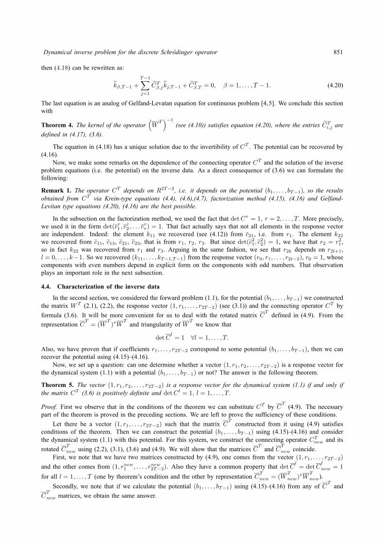
Dynamical inverse problem for the discrete Schrodinger operator 851
then (4.18) can be rewritten as:
kβ,T−1 +
T−1∑j=1
CTβ,j kj,T−1 + CTβ,T = 0, β = 1, . . . , T − 1. (4.20)
The last equation is an analog of Gelfand-Levatan equation for continuous problem [4,5]. We conclude this sectionwith
Theorem 4. The kernel of the operator(W
T)−1
(see (4.10)) satisfies equation (4.20), where the entries CTi,j are
defined in (4.17), (3.6).
The equation in (4.18) has a unique solution due to the invertibility of CT . The potential can be recovered by(4.16).
Now, we make some remarks on the dependence of the connecting operator CT and the solution of the inverseproblem equations (i.e. the potential) on the inverse data. As a direct consequence of (3.6) we can formulate thefollowing:
Remark 1. The operator CT depends on R2T−2, i.e. it depends on the potential (b1, . . . , bT−1), so the resultsobtained from CT via Krein-type equations (4.4), (4.6),(4.7), factorization method (4.15), (4.16) and Gelfand-Levitan type equations (4.20), (4.16) are the best possible.
In the subsection on the factorization method, we used the fact that detCτ = 1, τ = 2, . . . , T . More precisely,we used it in the form det(cτ1 , c
τ2 , . . . c
ττ ) = 1. That fact actually says that not all elements in the response vector
are independent. Indeed: the element k11 we recovered (see (4.12)) from c21, i.e. from r1. The element k22we recovered from c11, c13, c21, c23, that is from r1, r2, r3. But since det(c21, c
22) = 1, we have that r2 = r21 ,
so in fact k22 was recovered from r1 and r3. Arguing in the same fashion, we see that r2k depends on r2l+1,l = 0, . . . , k−1. So we recovered (k11, . . . , kT−1,T−1) from the response vector (r0, r1, . . . , r2t−2), r0 = 1, whosecomponents with even numbers depend in explicit form on the components with odd numbers. That observationplays an important role in the next subsection.
4.4. Characterization of the inverse data
In the second section, we considered the forward problem (1.1), for the potential (b1, . . . , bT−1) we constructedthe matrix WT (2.1), (2.2), the response vector (1, r1, . . . , r2T−2) (see (3.1)) and the connecting operator CT by
formula (3.6). It will be more convenient for us to deal with the rotated matrix CT
defined in (4.9). From the
representation CT= (W
T)∗W
Tand triangularity of W
Twe know that
detCl= 1 ∀l = 1, . . . , T.
Also, we have proven that if coefficients r1, . . . , r2T−2 correspond to some potential (b1, . . . , bT−1), then we canrecover the potential using (4.15)–(4.16).
Now, we set up a question: can one determine whether a vector (1, r1, r2, . . . , r2T−2) is a response vector forthe dynamical system (1.1) with a potential (b1, . . . , bT−1) or not? The answer is the following theorem.
Theorem 5. The vector (1, r1, r2, . . . , r2T−2) is a response vector for the dynamical system (1.1) if and only ifthe matrix CT (3.6) is positively definite and detCl = 1, l = 1, . . . , T .
Proof. First we observe that in the conditions of the theorem we can substitute CT by CT
(4.9). The necessarypart of the theorem is proved in the preceding sections. We are left to prove the sufficiency of these conditions.
Let there be a vector (1, r1, . . . , r2T−2) such that the matrix CT
constructed from it using (4.9) satisfiesconditions of the theorem. Then we can construct the potential (b1, . . . , bT−1) using (4.15)–(4.16) and considerthe dynamical system (1.1) with this potential. For this system, we construct the connecting operator CTnew and its
rotated CT
new using (2.2), (3.1), (3.6) and (4.9). We will show that the matrices CT
and CT
new coincide.First, we note that we have two matrices constructed by (4.9), one comes from the vector (1, r1, . . . , r2T−2)
and the other comes from (1, rnew1 , . . . , rnew2T−2). Also they have a common property that detCl= detC
l
new = 1
for all l = 1, . . . , T (one by theorem’s condition and the other by representation CT
new = (WT
new)∗W
T
new).
Secondly, we note that if we calculate the potential (b1, . . . , bT−1) using (4.15)–(4.16) from any of CT
and
CT
new matrices, we obtain the same answer.
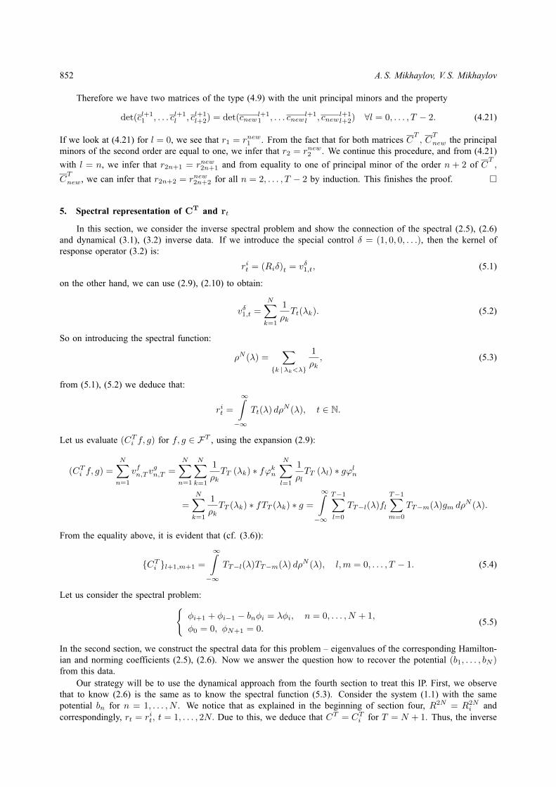
852 A. S. Mikhaylov, V. S. Mikhaylov
Therefore we have two matrices of the type (4.9) with the unit principal minors and the property
det(cl+11 , . . . cl+1
l , cl+1l+2) = det(cnew
l+11 , . . . cnew
l+1l , cnew
l+1l+2) ∀l = 0, . . . , T − 2. (4.21)
If we look at (4.21) for l = 0, we see that r1 = rnew1 . From the fact that for both matrices CT, C
T
new the principalminors of the second order are equal to one, we infer that r2 = rnew2 . We continue this procedure, and from (4.21)
with l = n, we infer that r2n+1 = rnew2n+1 and from equality to one of principal minor of the order n + 2 of CT,
CT
new, we can infer that r2n+2 = rnew2n+2 for all n = 2, . . . , T − 2 by induction. This finishes the proof.
5. Spectral representation of CT and rt
In this section, we consider the inverse spectral problem and show the connection of the spectral (2.5), (2.6)and dynamical (3.1), (3.2) inverse data. If we introduce the special control δ = (1, 0, 0, . . .), then the kernel ofresponse operator (3.2) is:
rit = (Riδ)t = vδ1,t, (5.1)
on the other hand, we can use (2.9), (2.10) to obtain:
vδ1,t =
N∑k=1
1
ρkTt(λk). (5.2)
So on introducing the spectral function:
ρN (λ) =∑
k |λk<λ
1
ρk, (5.3)
from (5.1), (5.2) we deduce that:
rit =
∞∫−∞
Tt(λ) dρN (λ), t ∈ N.
Let us evaluate (CTi f, g) for f, g ∈ FT , using the expansion (2.9):
(CTi f, g) =
N∑n=1
vfn,T vgn,T =
N∑n=1
N∑k=1
1
ρkTT (λk) ∗ fϕkn
N∑l=1
1
ρlTT (λl) ∗ gϕln
=
N∑k=1
1
ρkTT (λk) ∗ fTT (λk) ∗ g =
∞∫−∞
T−1∑l=0
TT−l(λ)fl
T−1∑m=0
TT−m(λ)gm dρN (λ).
From the equality above, it is evident that (cf. (3.6)):
CTi l+1,m+1 =
∞∫−∞
TT−l(λ)TT−m(λ) dρN (λ), l,m = 0, . . . , T − 1. (5.4)
Let us consider the spectral problem:φi+1 + φi−1 − bnφi = λφi, n = 0, . . . , N + 1,
φ0 = 0, φN+1 = 0.(5.5)
In the second section, we construct the spectral data for this problem – eigenvalues of the corresponding Hamilton-ian and norming coefficients (2.5), (2.6). Now we answer the question how to recover the potential (b1, . . . , bN )from this data.
Our strategy will be to use the dynamical approach from the fourth section to treat this IP. First, we observethat to know (2.6) is the same as to know the spectral function (5.3). Consider the system (1.1) with the samepotential bn for n = 1, . . . , N . We notice that as explained in the beginning of section four, R2N = R2N
i andcorrespondingly, rt = rit, t = 1, . . . , 2N. Due to this, we deduce that CT = CTi for T = N + 1. Thus, the inverse
Dynamical inverse problem for the discrete Schrodinger operator 853
problem can be solved in the following way: from the spectral data (2.6), we construct the spectral functionby (5.3). Then, we construct:
rt = rit =
∞∫−∞
Tt(λ) dρN (λ), t = 1, . . . , 2N,
CTlm = CTi l+1,m+1 =
∞∫−∞
TT−l(λ)TT−m(λ) dρN (λ), l,m = 0, . . . , N − 1.
After we have in hands the connecting operator, we can use the methods of section four to find (b1, . . . , bN ).
Acknowledgements
The research of Victor Mikhaylov was supported in part by NIR SPbGU 11.38.263.2014 and RFBR 14-01-00535. Alexandr Mikhaylov was supported by RFBR 14-01-00306; A. S. Mikhaylov and V. S. Mikhaylov werepartly supported by VW Foundation program ‘Modeling, Analysis, and Approximation Theory toward applicationin tomography and inverse problems’.
References
[1] Belishev M.I. Recent progress in the boundary control method. Inverse Problems, 2007, 23 (5), R1.[2] Avdonin S.A., Mikhaylov A.S., Mikhaylov V.S. On some applications of the Boundary Control method to spectral estimation and inverse
problems. Nanosystems: Phys. Chem. Math., 2015, 6 (1), P. 63–78.[3] Belishev M.I. C*-Algebras in reconstruction of manifolds. Nanosystems: Phys. Chem. Math., 2013, 4 (4), P. 484–489.[4] Avdonin S.A., Mikhaylov V.S. The boundary control approach to inverse spectral theory. Inverse Problems, 2010, 26 (4), 045009, 19 p.[5] Belishev M.I., Mikhailov V.S. Unified approach to classical equations of inverse problem theory. Journal of Inverse and Ill-Posed
Problems, 2012, 20 (4), P. 461–488.
NANOSYSTEMS: PHYSICS, CHEMISTRY, MATHEMATICS, 2016, 7 (5), P. 854–864
On direct and inverse spectral problems for sloshingof a two-layer fluid in an open container
N. G. Kuznetsov
Laboratory for Mathematical Modelling of Wave Phenomena,Institute for Problems in Mechanical Engineering, Russian Academy of Sciences,
V. O., Bol’shoy pr. 61, St. Petersburg, 199178, Russian Federation
PACS 02.30.Jr, 47.35.Bb DOI 10.17586/2220-8054-2016-7-5-854-864
We study the direct and inverse eigenvalue problems for a pair of harmonic functions with a spectral parameter in boundary and couplingconditions. The direct problem is relevant to sloshing frequencies of free oscillations of a two-layer fluid in a container. The upper fluidoccupies a layer bounded above by a free surface and below by a layer of fluid of greater density. Both fluids are assumed to be inviscid,incompressible, and heavy, whereas the free surface and the interface between fluids are considered bounded.
Keywords: Laplace equation, sloshing problem, two-layer fluid, eigenvalue, eigenfunction, inverse spectral problem.
Received: 19 August 2016
Revised: 5 September 2016
In memory of B. S. Pavlov (1936–2016)
1. Introduction
Linear water wave theory is a widely used approach for describing the behavior of surface waves in thepresence of rigid boundaries. In particular, this theory is a common tool for determining sloshing frequenciesand modes in containers occupied by a homogeneous fluid, that is, having constant density. The correspondingboundary spectral problem, usually referred to as the sloshing problem, has been the subject of a great number ofstudies over more than two centuries (a historical review can be found, for example, in [1]). In the comprehensivebook [2], an advanced technique based on spectral theory of operators in a Hilbert space was presented for studyingthis problem.
In the framework of the mathematical theory of linear water waves, substantial work has been done in thepast two decades for understanding the difference between the results valid for homogeneous and two-layer fluids(in the latter case the upper fluid occupies a layer bounded above by a free surface and below by a layer of fluidwhose density is greater than that in the upper one). These results concern wave/structure interactions and trappingof waves by immersed bodies (see, for example, [3–5] and references cited therein), but much less is known aboutthe difference between sloshing in containers occupied by homogeneous and two-layer fluids. To the author’sknowledge, there is only one related paper [6] with rigorous results for multilayered fluids, but it deals only withthe spectral asymptotics in a closed container. Thus, the first aim of the present paper is to fill in this gap at leastpartially.
Another aim is to consider the so-called inverse sloshing problem; that is, the problem of recovering somephysical parameters from known spectral data. The parameters to be recovered are the depth of the interfacebetween the two layers and the density ratio that characterizes stratification. It is demonstrated that for determiningthese two characteristics for fluids occupying a vertical-walled container with a horizontal bottom, one has tomeasure not only the two smallest sloshing eigenfrequencies, which must satisfy certain inequalities, but also toanalyze the corresponding free surface elevations.
1.1. Statement of the direct problem
Let two immiscible, inviscid, incompressible, heavy fluids occupy an open container whose walls and bottomare rigid surfaces. We choose rectangular Cartesian coordinates (x1, x2, y) so that their origin lies in the mean freesurface of the upper fluid and the y-axis is directed upwards. Then, the whole fluid domain W is a subdomain ofthe lower half-space −∞ < x1, x2 < +∞, y < 0. The boundary ∂W is assumed to be piece-wise smooth andsuch that every two adjacent smooth pieces of ∂W are not tangent along their common edge. We also supposethat each horizontal cross-section of W is a bounded two-dimensional domain; that is, a connected, open setin the corresponding plane. (The latter assumption is made for the sake of simplicity because it excludes thepossibility of two or more interfaces between fluids at different levels.) The free surface F bounding above the
Direct and inverse spectral problems for sloshing of a two-layer fluid 855
upper fluid of density ρ1 > 0 is the non-empty interior of ∂W ∩ y = 0. The interface I = W ∩ y = −h,where 0 < h < max|y| : (x1, x2, y) ∈ ∂W, separates the upper fluid from the lower one of density ρ2 > ρ1.We denote by W1 and W2 the domains W ∩ y > −h and W ∩ y < −h respectively; they are occupied bythe upper and lower fluids respectively. The surface tension is neglected and we suppose the fluid motion to beirrotational and of small amplitude. Therefore, the boundary conditions on F and I may be linearized. With atime-harmonic factor, say cosωt, removed, the velocity potentials u(1)(x1, x2, y) and u(2)(x1, x2, y) (they may betaken to be real functions) for the flow in W1 and W2 respectively must satisfy the following coupled boundaryvalue problem:
u(j)x1x1+ u(j)x2x2
+ u(j)yy = 0 in Wj , j = 1, 2, (1)
u(1)y = νu(1) on F, (2)
ρ(u(2)y − νu(2)
)= u(1)y − νu(1) on I, (3)
u(2)y = u(1)y on I, (4)
∂u(j)/∂n = 0 on Bj j = 1, 2. (5)
Here, ρ = ρ2/ρ1 > 1 is the non-dimensional measure of stratification, the spectral parameter ν is equal to ω2/g,where ω is the radian frequency of the water oscillations and g is the acceleration due to gravity; Bj = ∂Wj\(F∪I)is the rigid boundary of Wj . By combining (3) and (4), we get another form of the spectral coupling condition (3):
(ρ− 1)u(2)y = ν(ρu(2) − u(1)
)on I. (6)
We also suppose that the orthogonality conditions∫F
u(1) dx = 0 and
∫I
(ρu(2) − u(1)
)dx = 0, dx = dx1dx2, (7)
hold, thus excluding the zero eigenvalue of (1)–(5).When ρ = 1, conditions (3) and (4) mean that the functions u(1) and u(2) are harmonic continuations of each
other across the interface I . Then, problem (1)–(5) complemented by the first orthogonality condition (7) (thesecond condition (7) is trivial), becomes the usual sloshing problem for a homogeneous fluid. It is well-knownsince the 1950s that the latter problem has a positive discrete spectrum. This means that there exists a sequence ofpositive eigenvalues νWn ∞1 of finite multiplicity (the superscript W is used here and below for distinguishing thesloshing eigenvalues that correspond to the case, when a homogeneous fluid occupies the whole domain W , fromthose corresponding to a two-layer fluid which will be denoted simply by νn). In this sequence the eigenvaluesare written in increasing order and repeated according to their multiplicity; moreover, νWn → ∞ as n → ∞. Thecorresponding eigenfunctions un∞1 ⊂ H1(W ) form a complete system in an appropriate Hilbert space. Theseresults can be found in many sources, for example, in the book [2].
2. Variational principle
Let W be bounded. It is well known that the sloshing problem in W for homogeneous fluid can be cast intothe form of a variational problem and the corresponding Rayleigh quotient is as follows:
RW (u) =
∫W
|∇u|2 dxy∫F
u2 dx. (8)
In order to obtain the fundamental eigenvalue νW1 one has to minimize RW (u) over the subspace of theSobolev space H1(W ) consisting of functions that satisfy the first orthogonality condition (7). To find νWn forn > 1, one has to minimize (8) over the subspace of H1(W ) such that each of its element u satisfies thefirst condition (7) along with the following equalities
∫F
uuj dx = 0, where uj is either of the eigenfunctions
u1, . . . , un−1 corresponding to the eigenvalues νW1 , . . . , νWn−1.In the case of a two-layer fluid, we assume that the usual embedding theorems hold for both subdomains Wj ,
j = 1, 2 (the theorem about traces on smooth pieces of the boundary for elements of H1 included). This imposessome restrictions on ∂W , in particular, on the character of the intersections of F and I with ∂W ∩ y < 0. Then
856 N. G. Kuznetsov
using (6), it is easy to verify that the Rayleigh quotient for the two-layer sloshing problem has the following form:
R(u(1), u(2)) =
∫W1
∣∣∇u(1)∣∣2 dxdy + ρ∫W2
∣∣∇u(2)∣∣2 dxdy∫F
[u(1)
]2dx+ (ρ− 1)−1
∫I
[ρu(2) − u(1)
]2dx. (9)
To determine the fundamental sloshing eigenvalue ν1 one has to minimize R(u(1), u(2)) over the subspace ofH1(W1) ⊕ H1(W2) defined by both orthogonality conditions (7). In order to find νn for n > 1, one has tominimize (9) over the subspace of H1(W1) ⊕ H1(W2) such that every element
(u(1), u(2)
)of this subspace
satisfies the equalities:∫F
u(1) u(1)j dx = 0 and
∫I
[ρu(2) − u(1)
] [ρu
(2)j − u
(1)j
]dx = 0, j = 1, . . . , n− 1,
along with both conditions (7). Here,(u(1)j , u
(2)j
)is either of the eigensolutions corresponding to ν1, . . . , νn−1.
Now we are in a position to prove the following assertion.
Proposition 1. Let νW1 and ν1 be the fundamental eigenvalues of the sloshing problem in the bounded domainW for homogeneous and two-layer fluids respectively. Then the inequality ν1 < νW1 holds.
The restriction that W is bounded is essential as the example considered in Proposition 4 below demonstrates.
Proof. If u1 is an eigenfunction corresponding to νW1 , then
νW1 =
∫W
|∇u1|2 dxdy∫F
u21 dx.
Let u(1) and u(2) be equal to the restrictions of ρu1 and u1 to W1 and W2, respectively. Then the pair(u(1), u(2)
)is an admissible element for the Rayleigh quotient (9). Substituting it into (9), we obtain that:
R(ρu1, u1) =
∫W1
|∇u1|2 dxdy + ρ−1∫W2
|∇u1|2 dxdy∫F
u21 dx.
Comparing this equality with the previous one and taking into account that ρ > 1, one finds thatR(ρu1, u1) < νW1 . Since ν1 is the minimum of (9), we conclude that ν1 < νW1 .
3. Containers with vertical walls and horizontal bottoms
Let us consider the fluid domain W = x = (x1, x2) ∈ D, y ∈ (−d, 0), where D is a piece-wise smoothtwo-dimensional domain (the container’s horizontal cross-section) and d ∈ (0,∞] is the container’s constant depth.Thus, the container’s side wall ∂D × (−d, 0) is vertical, the bottom x ∈ D, y = −d is horizontal, whereas thefree surface and the interface are F = x ∈ D, y = 0 and I = x ∈ D, y = −h respectively, 0 < h < d.
For a homogeneous fluid occupying such a container, the sloshing problem is equivalent to the free membraneproblem. Indeed, putting
u(x, y) = v(x) cosh k(y + d)(u(x, y) = v(x) eky when d =∞
),
one reduces problem (1)–(5) with ρ = 1, complemented by the first orthogonality condition (7) to the followingspectral problem:
∇2xv + k2v = 0 in D, ∂v/∂nx = 0 on ∂D,
∫D
v dx = 0, (10)
where ∇x = (∂/∂x1, ∂/∂x2) and nx is a unit normal to ∂D in R2. It is clear that νW is an eigenvalue of theformer problem if and only if k2 is an eigenvalue of (10) and
νW = k tanh kd when d <∞(νW = k when d =∞
), k > 0. (11)
It is well-known that problem (10) has a sequence of positive eigenvalues k2n∞1 written in increasing order andrepeated according to their finite multiplicity, and such that k2n →∞ as n→∞. The corresponding eigenfunctionsform a complete system in H1(D).
Direct and inverse spectral problems for sloshing of a two-layer fluid 857
Let us describe the same reduction procedure in the case when W is occupied by a two-layer fluid and d <∞.Putting
u(1)(x, y) = v(x) [A cosh k(y + h) +B sinh k(y + h)], (12)
u(2)(x, y) = v(x)C cosh k(y + d), (13)
where A,B and C are constants, one reduces problem (1)–(5) and (7), ρ > 1, to problem (10) combined with thefollowing quadratic equation:
ν2 cosh kd− νk [sinh kd+ (ρ− 1) cosh kh sinh k(d− h)]
+ k2(ρ− 1) sinh kh sinh k(d− h) = 0, k > 0. (14)
Thus ν is an eigenvalue of the former problem if and only if ν satisfies (14), where k2 is an eigenvalue of (10).Indeed, the quadratic polynomial in ν on the left-hand side of (14) is the determinant of the following linear
algebraic system for A, B and C:
A = C[cosh k(d− h)− ν−1(ρ− 1) k sinh k(d− h)
], B = C sinh k(d− h), (15)
A (k sinh kh− ν cosh kh) + C sinh k(d− h) (k cosh kh− ν sinh kh) = 0. (16)
The latter arises when one substitutes expressions (12) and (13) into the boundary condition (2) and the couplingconditions (3) and (4). This homogeneous system defines eigensolutions of the sloshing problem provided thereexists a non-trivial solution, and so the determinant must vanish which is expressed by (14).
Let us show that the roots ν(+) and ν(−) of (14) are real in which case
ν(±) = kb±√D
2 cosh kd> 0 , (17)
where the inequality is a consequence of the formulae:
b = sinh kd+ (ρ− 1) cosh kh sinh k(d− h), (18)
D = b2 − 4 (ρ− 1) cosh kd sinh kh sinh k(d− h). (19)
Since D is a quadratic polynomial of ρ− 1, it is a simple application of calculus to demonstrate that it attainsthe minimum at
ρ− 1 =2 cosh kd sinh kh− sinh kd cosh kh
cosh2 kh sinh k(d− h),
and after some algebra one finds that this minimum is equal to
4 cosh kd sinh kh sinh k(d− h)
cosh2 kh> 0,
which proves the assertion. Thus we arrive at the following.
Proposition 2. If W is a vertical cylinder with horizontal bottom, then the sloshing problem for a two-layer fluidoccupying W has two sequences of eigenvalues
ν(+)n
∞1
andν(−)n
∞1
defined by (17) with k = kn > 0, where k2n is an eigenvalue of problem (10).
The same eigensolution (u(1), u(2)) corresponds to both ν(+)n and ν(−)n , where u(1) and u(2) (sloshing modes
in W1 and W2 respectively) are defined by formulae (12) and (13) with v belonging to the set of eigenfunctionsof problem (10) that correspond to k2n; furthermore, C is an arbitrary non-zero real constant, whereas A and Bdepend on C through (15).
Next, we analyze the behavior of ν(±)n as a function of ρ.
Proposition 3. For every n = 1, 2, . . . the functions ν(−)n and ν(+)n are monotonically increasing as ρ goes from
1 to infinity. Their ranges are:
(0, kn tanh knh) and (kn tanh knd, ∞)
respectively.
858 N. G. Kuznetsov
Proof. In order to prove the proposition, it is sufficient to show that:
∂(b±√D )
∂ρ= sinh k(d− h)
cosh kh±D−1/2
[cosh kh sinh kd
+(ρ− 1) cosh2 kh sinh k(d− h)− 2 cosh kd sinh kh]
> 0 . (20)
Since∂(b+
√D )
∂ρ
∣∣∣∣∣ρ=1
=2 sinh2 k(d− h)
sinh kd> 0 and
∂(b−√D )
∂ρ
∣∣∣∣∣ρ→∞
= 0 ,
inequality (20) is a consequence of the following one:
±∂2(b±
√D )
∂ρ2=
4 cosh kd sinh kh sinh3 k(d− h)
D3/2> 0 for all ρ > 1.
The second assertion immediately follows from the first one and formulae (17)–(19).
Combining Proposition 3 and formula (11), we arrive at the following assertion.
Corollary 1. The inequalities ν(−)n < νWn < ν(+)n hold for each n = 1, 2, . . . and every ρ > 1.
Dividing (17) by k and letting k = kn to infinity, it is straightforward to obtain the following.
Lemma 1. For every ρ > 1, the asymptotic formula:
ν(±)n ∼ ρ+ 1± |ρ− 3|4
kn as n→∞,
holds with the exponentially small remainder term; here k2n is an eigenvalue of (10).
In other words, there are three cases:
(i) if ρ = 3, then ν(±)n ∼ kn as n→∞;
(ii) if ρ > 3, then ν(−)n ∼ kn and ν(+)n ∼ (ρ− 1) kn/2 as n→∞;
(iii) if ρ ∈ (1, 3), then ν(−)n ∼ (ρ− 1) kn/2 and ν(+)n ∼ kn as n→∞.
Combining these relations and the asymptotic formula νWn ∼ kn as n → ∞ (it is a consequence of formula (11)defining νWn when a homogeneous fluid occupies W ), we obtain the following.
Corollary 2. As n→∞, we have that ν(−)n ∼ νWn when ρ ≥ 3, whereas ν(+)n ∼ νWn provided ρ ∈ (1, 3].
Another corollary of Lemma 1 concerns the distribution function N (ν) for the spectrum of problem (1)–(5)and (7). This function is equal to the total number of eigenvalues νn that do not exceed ν. An asymptotic formulafor N (ν) immediately follows from Lemma 1 and the asymptotic formula for the distribution of the spectrum forthe Neumann Laplacian (see [7], Chapter 6).
Corollary 3. The distribution function N (ν) of the spectrum for the sloshing of a two-layer fluid in a verticalcylinder of cross-section D has the following asymptotics:
N (ν) ∼[
4
(ρ− 1)2+ 1
]|D| ν2
4πas ν →∞.
Here, |D| stands for the area of D.
It should be also mentioned that in [6] the asymptotics for N (ν) was obtained for a multi-layer fluid occupyinga bounded closed container.
It follows from Lemma 1 and Corollary 2 that the asymptotic formula for the distribution function of thespectrum
νWn∞1
is similar to the above one, but the first term in the square brackets must be deleted. Moreover,in the case of homogeneous fluid the same asymptotic formula (up to the remainder term) holds for arbitrarilyshaped fluid domains (see [2], Section 3.3). Since the first term in the square brackets tends to infinity as ρ→ 1,the transition from the two-layer fluid to the homogeneous one in the asymptotic formula for N (ν) is a singularlimit in the sense described in [8]. A similar effect occurs for modes trapped by submerged bodies in two-layerand homogeneous fluids as was noted in [4].
In conclusion of this section, it should be noted that in the case of an infinitely deep vertical cylinder it is easyto verify that ν = k is an eigenvalue of the sloshing problem for a two-layer fluid if and only if k2 is an eigenvalueof problem (10). Comparing this assertion with that at the beginning of this section, we obtain the following.
Direct and inverse spectral problems for sloshing of a two-layer fluid 859
Proposition 4. In an infinitely deep vertical-walled container, the sloshing problem for a two-layer fluid has thesame set of eigenvalues and the same eigenfunctions of the form v(x) eky , k > 0, as the sloshing problem for ahomogeneous fluid in the same container; here, k2 is an eigenvalue and v is the corresponding eigenfunction ofproblem (10).
4. Inverse problem
Let a given container W be occupied by a two-layer fluid, but now we assume that the position of the interfacebetween layers and the density of the lower layer are unknown. The density of the upper layer is known becauseone can measure it directly. The sequence of eigenvalues
νWn∞1
corresponding to the homogeneous fluid is alsoknown because it depends only on the domain W . The inverse problem we are going to consider is to recover theratio of densities ρ and the depth of the interface h from measuring some sloshing frequencies on the free surface.Thus, we let the fundamental eigenvalue ν1 be known along with the second-largest one.
The formulated inverse problem is not always solvable. Indeed, according to Proposition 4, it has no solutionwhen W is an infinitely deep container with vertical walls. Moreover, the inverse problem is trivial for all domainswhen ν1 = νW1 . In this case, Proposition 1 implies that the fluid is homogeneous, that is, ρ = 1 and h = d.Therefore, we restrict ourselves to the case of vertically-walled containers having a finite depth d in what follows.
4.1. Reduction to transcendental equations
In view of what was said above, the inverse problem for W = D × (−d, 0) can be stated as follows. Findconditions that allow us to determine ρ > 1 and h ∈ (0, d) when the following two eigenvalues are known: thefundamental one ν1 and the smallest eigenvalue νN that is greater than ν1. Thus, N is such that k2n = k21 forall n = 1, . . . , N − 1, which means that the fundamental eigenvalue k21 of problem (10) is of multiplicity N − 1(of course, ν1 has the same multiplicity). For example, if D is a disc, then the multiplicity of k21 is two (see [9],Section 3.1), and so νN = ν3 in this case.
According to formula (17), we have that ν1 = ν(−)1 . Hence the first equation for ρ and h is as follows:
b1 −√D1 =
2 ν1k1
cosh k1d. (21)
Here, b1 and D1 are given by formulae (18) and (19) respectively with k = k1.To write down the second equation for ρ and h, we have the dilemma whether
νN = ν(−)N or νN = ν
(+)1 ? (22)
Let us show that either of these options is possible. Indeed, Proposition 3 implies that νN = ν(−)N provided ρ− 1
is sufficiently small. On the other hand, let us demonstrate that there exists a triple (ρ, d, h) for which νN = ν(+)1 .
For this purpose we have to demonstrate that the inequality
ν(−)N = kN
bN −√DN
2 cosh kNd≥ k1
b1 +√D1
2 cosh k1d= ν
(+)1
holds for some ρ, d and h. As above bj and Dj , j = 1, N , are given by formulae (18) and (19), respectively, withk = kj .
Let h = d/2, then we have:
4 ν(±)j = kj
(ρ+ 1) tanh kjd±
[(ρ+ 1)2 tanh2 kjd+ 8 (ρ− 1)
1− cosh kjd
cosh kjd
]1/2,
and so4[ν(−)N − ν(+)
1
]→ kN (ρ+ 1− |ρ− 3|)− k1 (ρ+ 1 + |ρ− 3|) as d→∞.
The limit is piecewise linear function of ρ, attains its maximum value 4(kN − k1) at ρ = 3 and is positive forρ ∈ (1 + 2 (k1/kN ), 1 + 2 (kN/k1)).
Summarizing, we arrive at the following.
Proposition 5. Let k2N be the smallest eigenvalue of problem (10) other than k21 , and let ν(−)N be the sloshingeigenvalue defined by (17)–(19) with k = kN . Then
(i) ν(−)N < ν(+)1 when ρ − 1 > 0 is sufficiently small (of course, its value depends on d, h and the domain
D);
(ii) ν(−)N > ν(+)1 when ρ ∈ (1 + 2 (k1/kN ), 1 + 2 (kN/k1)), h = d/2 and d is sufficiently large (of course, its
value depends on ρ and D).
860 N. G. Kuznetsov
Obviously, assertion (ii) can be extended to values of h that are sufficiently close to d/2.
4.2. Options for the second equation
Let us develop a procedure for determining which of the two equalities (22) can be chosen to complementequation (21) in order to find ρ and h. Our procedure is based on an analysis of the free surface elevationscorresponding to the measured values ν1 and νN . Indeed, when a two-layer fluid oscillates at the frequencydefined by some νj , the free surface elevation is proportional to the trace u
(1)j (x, 0) (see, for example, [10],
Section 227).
According to formula (12), the trace u(1)1 (x, 0) is a linear combination of linearly independent eigenfunctionsv1(x), . . . , vN−1(x) corresponding to the fundamental eigenvalue k21 of problem (10); of course, its multiplicity
is taken into account. By Proposition 2 the free surface elevation associated with ν(+)1 is also proportional to a
linear combination of v1, . . . , vN−1. Since these functions are known, one has to determine whether the measuredfree-surface elevation corresponding to νN can be represented in the form of such a combination and only in sucha form. If this is the case, then νN = ν
(+)1 < ν
(−)N and the following equation:
b1 +√D1 =
2 νNk1
cosh k1d (23)
forms the system for ρ and h together with (21).Besides, it can occur that the measured free-surface elevation corresponding to νN is representable in two
forms, one of which is a linear combination of v1, . . . , vN−1, whereas the other one involves the function vN aswell as other eigenfunctions corresponding to the eigenvalue k2N of problem (10) along with v1, . . . , vN−1. It is
clear that this happens when νN = ν(+)1 = ν
(−)N . Indeed, if all coefficients at the eigenfunctions of k2N vanish,
then the profile is represented by v1, . . . , vN−1, otherwise not. In this case, equation (21) can be complemented byeither equation (23) or the following one:
bN −√DN =
2 νNkN
cosh kNd. (24)
Of course, it is better to use the system that comprises equations (21) and (23) because the right-hand side termsin these equations are proportional.
If the measured free-surface elevation corresponding to νN cannot be represented as a linear combination ofv1, . . . , vN−1, then νN = ν
(−)N < ν
(+)1 , in which case the elevation is a linear combination of eigenfunctions that
correspond to the eigenvalue k2N of problem (10) the second largest after k21 . In this case, equation (21) must becomplemented by (24).
Thus, we arrive at the following procedure for reducing the inverse sloshing problem to a system of twoequations.
Procedure. Let v1, . . . , vN−1 be the set of linearly independent eigenfunctions of problem (10) corresponding tok21 . If the observed elevation of the free surface that corresponds to the measured value νN has a representation asa linear combination of v1, . . . , vN−1, then ρ and d must be determined from equations (21) and (23). Otherwise,equations (21) and (24) must be used.
The simplest case is when the fundamental eigenvalue of problem (10) is simple, that is, N = 2. Thenthe above procedure reduces to examining whether the free surface elevations corresponding to ν1 and ν2 areproportional or not. In the case of proportionality, equations (21) and (23) must be used. Equations (21) and (24)are applicable when there is no proportionality.
5. Solution of the transcendental systems
In this section, we consider the question how to solve systems (21) and (24), and (21) and (23) for finding ρand h.
5.1. System (21) and (23)
Equations (21) and (23) can be easily simplified. Indeed, the sum and difference of these equations are asfollows:
b1 =νN + ν1k1
cosh k1d and D1 =
(νN − ν1k1
)2
cosh2 k1d .
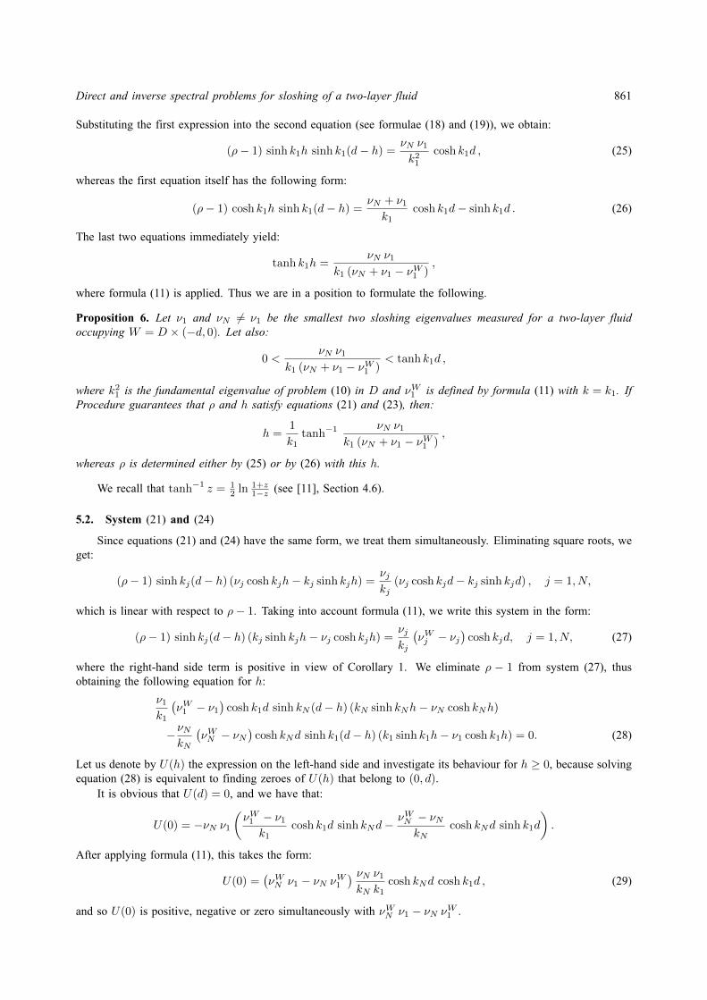
Direct and inverse spectral problems for sloshing of a two-layer fluid 861
Substituting the first expression into the second equation (see formulae (18) and (19)), we obtain:
(ρ− 1) sinh k1h sinh k1(d− h) =νN ν1k21
cosh k1d , (25)
whereas the first equation itself has the following form:
(ρ− 1) cosh k1h sinh k1(d− h) =νN + ν1k1
cosh k1d− sinh k1d . (26)
The last two equations immediately yield:
tanh k1h =νN ν1
k1 (νN + ν1 − νW1 ),
where formula (11) is applied. Thus we are in a position to formulate the following.
Proposition 6. Let ν1 and νN 6= ν1 be the smallest two sloshing eigenvalues measured for a two-layer fluidoccupying W = D × (−d, 0). Let also:
0 <νN ν1
k1 (νN + ν1 − νW1 )< tanh k1d ,
where k21 is the fundamental eigenvalue of problem (10) in D and νW1 is defined by formula (11) with k = k1. IfProcedure guarantees that ρ and h satisfy equations (21) and (23), then:
h =1
k1tanh−1
νN ν1k1 (νN + ν1 − νW1 )
,
whereas ρ is determined either by (25) or by (26) with this h.
We recall that tanh−1 z = 12 ln 1+z
1−z (see [11], Section 4.6).
5.2. System (21) and (24)
Since equations (21) and (24) have the same form, we treat them simultaneously. Eliminating square roots, weget:
(ρ− 1) sinh kj(d− h) (νj cosh kjh− kj sinh kjh) =νjkj
(νj cosh kjd− kj sinh kjd) , j = 1, N,
which is linear with respect to ρ− 1. Taking into account formula (11), we write this system in the form:
(ρ− 1) sinh kj(d− h) (kj sinh kjh− νj cosh kjh) =νjkj
(νWj − νj
)cosh kjd, j = 1, N, (27)
where the right-hand side term is positive in view of Corollary 1. We eliminate ρ − 1 from system (27), thusobtaining the following equation for h:
ν1k1
(νW1 − ν1
)cosh k1d sinh kN (d− h) (kN sinh kNh− νN cosh kNh)
−νNkN
(νWN − νN
)cosh kNd sinh k1(d− h) (k1 sinh k1h− ν1 cosh k1h) = 0. (28)
Let us denote by U(h) the expression on the left-hand side and investigate its behaviour for h ≥ 0, because solvingequation (28) is equivalent to finding zeroes of U(h) that belong to (0, d).
It is obvious that U(d) = 0, and we have that:
U(0) = −νN ν1(νW1 − ν1
k1cosh k1d sinh kNd−
νWN − νNkN
cosh kNd sinh k1d
).
After applying formula (11), this takes the form:
U(0) =(νWN ν1 − νN νW1
) νN ν1kN k1
cosh kNd cosh k1d , (29)
and so U(0) is positive, negative or zero simultaneously with νWN ν1 − νN νW1 .
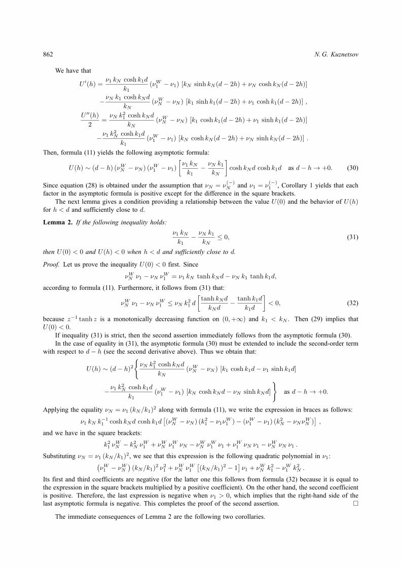
862 N. G. Kuznetsov
We have that
U ′(h) =ν1 kN cosh k1d
k1(νW1 − ν1) [kN sinh kN (d− 2h) + νN cosh kN (d− 2h)]
−νN k1 cosh kNd
kN(νWN − νN ) [k1 sinh k1(d− 2h) + ν1 cosh k1(d− 2h)] ,
U ′′(h)
2=νN k
21 cosh kNd
kN(νWN − νN ) [k1 cosh k1(d− 2h) + ν1 sinh k1(d− 2h)]
−ν1 k2N cosh k1d
k1(νW1 − ν1) [kN cosh kN (d− 2h) + νN sinh kN (d− 2h)] .
Then, formula (11) yields the following asymptotic formula:
U(h) ∼ (d− h) (νWN − νN ) (νW1 − ν1)
[ν1 kNk1
− νN k1kN
]cosh kNd cosh k1d as d− h→ +0. (30)
Since equation (28) is obtained under the assumption that νN = ν(−)N and ν1 = ν
(−)1 , Corollary 1 yields that each
factor in the asymptotic formula is positive except for the difference in the square brackets.The next lemma gives a condition providing a relationship between the value U(0) and the behavior of U(h)
for h < d and sufficiently close to d.
Lemma 2. If the following inequality holds:
ν1 kNk1
− νN k1kN
≤ 0, (31)
then U(0) < 0 and U(h) < 0 when h < d and sufficiently close to d.
Proof. Let us prove the inequality U(0) < 0 first. Since
νWN ν1 − νN νW1 = ν1 kN tanh kNd− νN k1 tanh k1d,
according to formula (11). Furthermore, it follows from (31) that:
νWN ν1 − νN νW1 ≤ νN k21 d[
tanh kNd
kNd− tanh k1d
k1d
]< 0, (32)
because z−1 tanh z is a monotonically decreasing function on (0,+∞) and k1 < kN . Then (29) implies thatU(0) < 0.
If inequality (31) is strict, then the second assertion immediately follows from the asymptotic formula (30).In the case of equality in (31), the asymptotic formula (30) must be extended to include the second-order term
with respect to d− h (see the second derivative above). Thus we obtain that:
U(h) ∼ (d− h)2
νN k
21 cosh kNd
kN(νWN − νN ) [k1 cosh k1d− ν1 sinh k1d]
−ν1 k2N cosh k1d
k1(νW1 − ν1) [kN cosh kNd− νN sinh kNd]
as d− h→ +0.
Applying the equality νN = ν1 (kN/k1)2 along with formula (11), we write the expression in braces as follows:
ν1 kN k−11 cosh kNd cosh k1d
[(νWN − νN ) (k21 − ν1νW1 )− (νW1 − ν1) (k2N − νNνWN )
],
and we have in the square brackets:
k21 νWN − k2N νW1 + νWN νW1 νN − νWN νW1 ν1 + νW1 νN ν1 − νWN νN ν1 .
Substituting νN = ν1 (kN/k1)2, we see that this expression is the following quadratic polynomial in ν1:(νW1 − νWN
)(kN/k1)2 ν21 + νWN νW1
[(kN/k1)2 − 1
]ν1 + νWN k21 − νW1 k2N .
Its first and third coefficients are negative (for the latter one this follows from formula (32) because it is equal tothe expression in the square brackets multiplied by a positive coefficient). On the other hand, the second coefficientis positive. Therefore, the last expression is negative when ν1 > 0, which implies that the right-hand side of thelast asymptotic formula is negative. This completes the proof of the second assertion.
The immediate consequences of Lemma 2 are the following two corollaries.
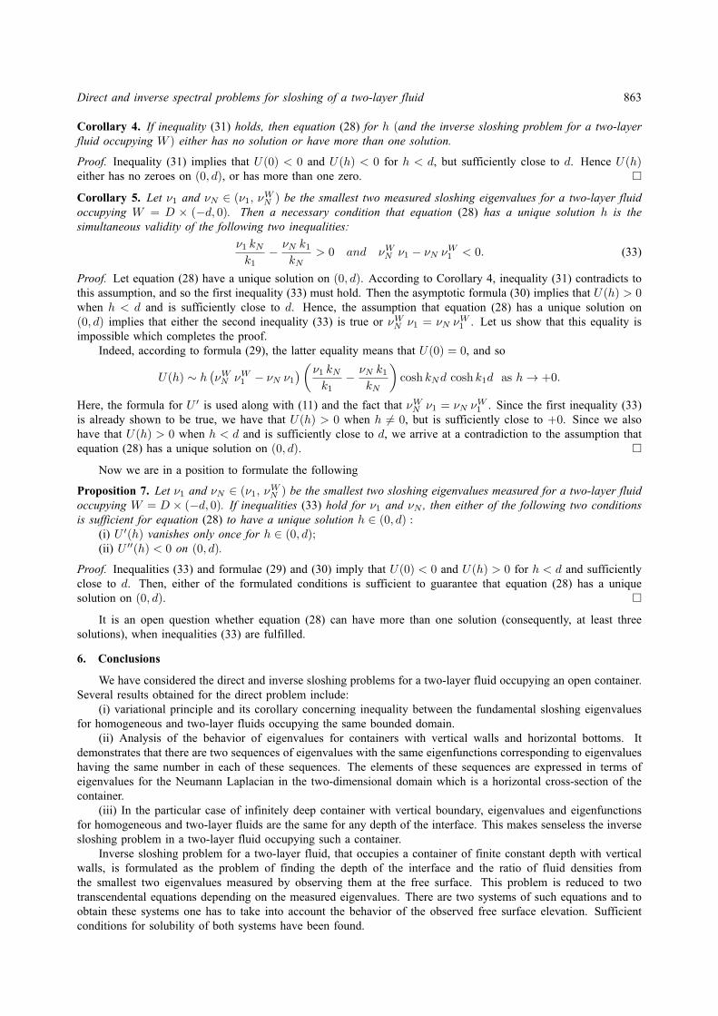
Direct and inverse spectral problems for sloshing of a two-layer fluid 863
Corollary 4. If inequality (31) holds, then equation (28) for h (and the inverse sloshing problem for a two-layerfluid occupying W ) either has no solution or have more than one solution.
Proof. Inequality (31) implies that U(0) < 0 and U(h) < 0 for h < d, but sufficiently close to d. Hence U(h)either has no zeroes on (0, d), or has more than one zero.
Corollary 5. Let ν1 and νN ∈ (ν1, νWN ) be the smallest two measured sloshing eigenvalues for a two-layer fluid
occupying W = D × (−d, 0). Then a necessary condition that equation (28) has a unique solution h is thesimultaneous validity of the following two inequalities:
ν1 kNk1
− νN k1kN
> 0 and νWN ν1 − νN νW1 < 0. (33)
Proof. Let equation (28) have a unique solution on (0, d). According to Corollary 4, inequality (31) contradicts tothis assumption, and so the first inequality (33) must hold. Then the asymptotic formula (30) implies that U(h) > 0when h < d and is sufficiently close to d. Hence, the assumption that equation (28) has a unique solution on(0, d) implies that either the second inequality (33) is true or νWN ν1 = νN ν
W1 . Let us show that this equality is
impossible which completes the proof.Indeed, according to formula (29), the latter equality means that U(0) = 0, and so
U(h) ∼ h(νWN νW1 − νN ν1
)(ν1 kNk1
− νN k1kN
)cosh kNd cosh k1d as h→ +0.
Here, the formula for U ′ is used along with (11) and the fact that νWN ν1 = νN νW1 . Since the first inequality (33)
is already shown to be true, we have that U(h) > 0 when h 6= 0, but is sufficiently close to +0. Since we alsohave that U(h) > 0 when h < d and is sufficiently close to d, we arrive at a contradiction to the assumption thatequation (28) has a unique solution on (0, d).
Now we are in a position to formulate the following
Proposition 7. Let ν1 and νN ∈ (ν1, νWN ) be the smallest two sloshing eigenvalues measured for a two-layer fluid
occupying W = D × (−d, 0). If inequalities (33) hold for ν1 and νN , then either of the following two conditionsis sufficient for equation (28) to have a unique solution h ∈ (0, d) :
(i) U ′(h) vanishes only once for h ∈ (0, d);(ii) U ′′(h) < 0 on (0, d).
Proof. Inequalities (33) and formulae (29) and (30) imply that U(0) < 0 and U(h) > 0 for h < d and sufficientlyclose to d. Then, either of the formulated conditions is sufficient to guarantee that equation (28) has a uniquesolution on (0, d).
It is an open question whether equation (28) can have more than one solution (consequently, at least threesolutions), when inequalities (33) are fulfilled.
6. Conclusions
We have considered the direct and inverse sloshing problems for a two-layer fluid occupying an open container.Several results obtained for the direct problem include:
(i) variational principle and its corollary concerning inequality between the fundamental sloshing eigenvaluesfor homogeneous and two-layer fluids occupying the same bounded domain.
(ii) Analysis of the behavior of eigenvalues for containers with vertical walls and horizontal bottoms. Itdemonstrates that there are two sequences of eigenvalues with the same eigenfunctions corresponding to eigenvalueshaving the same number in each of these sequences. The elements of these sequences are expressed in terms ofeigenvalues for the Neumann Laplacian in the two-dimensional domain which is a horizontal cross-section of thecontainer.
(iii) In the particular case of infinitely deep container with vertical boundary, eigenvalues and eigenfunctionsfor homogeneous and two-layer fluids are the same for any depth of the interface. This makes senseless the inversesloshing problem in a two-layer fluid occupying such a container.
Inverse sloshing problem for a two-layer fluid, that occupies a container of finite constant depth with verticalwalls, is formulated as the problem of finding the depth of the interface and the ratio of fluid densities fromthe smallest two eigenvalues measured by observing them at the free surface. This problem is reduced to twotranscendental equations depending on the measured eigenvalues. There are two systems of such equations and toobtain these systems one has to take into account the behavior of the observed free surface elevation. Sufficientconditions for solubility of both systems have been found.

864 N. G. Kuznetsov
References
[1] Fox D. W., Kuttler J. R. Sloshing frequencies. Z. angew. Math. Phys., 1983, 34, P. 668–696.[2] Kopachevsky N. D., Krein S. G. Operator Approach to Linear Problems of Hydrodynamics. Birkhauser, Basel – Boston – Berlin, 2001,
384 pp.[3] Cadby J. R., Linton C. M. Three-dimensional water-wave scattering in two-layer fluids. J. Fluid Mech., 2000, 423, P. 155–173.[4] Linton C. M., Cadby J. R. Trapped modes in a two-layer fluid. J. Fluid Mech., 2003, 481, P. 215–234.[5] Kuznetsov N., McIver M., McIver P. Wave interaction with two-dimensional bodies floating in a two-layer fluid: uniqueness and trapped
modes. J. Fluid Mech., 2003, 490, P. 321–331.[6] Karazeeva N. A., Solomyak M. Z. Asymptotics of the spectrum of the contact problem for elliptic equations of the second order. Selecta
Math. Sovietica, 1987, 6 (1), P. 151–161.[7] Courant R., Hilbert D. Methods of Mathematical Physics. Vol. 1. Interscience, N Y, 1953, 561 pp.[8] Berry M. Singular limits. Physics Today, 2002, 5, P. 10–11.[9] Bandle C. Isoperimetric Inequalities and Applications. Pitman, London, 1980, 228 pp.
[10] Lamb H. Hydrodynamics. Cambridge University Press, Cambridge, 1932, 738 pp.[11] Abramowitz M., Stegun I. A. Handbook of Mathematical Functions. Dover, Mineola, N Y, 1965, 1046 pp.
NANOSYSTEMS: PHYSICS, CHEMISTRY, MATHEMATICS, 2016, 7 (5), P. 865–868
Computer simulation of periodic nanostructures
E. N. Grishanov1, I. Y. Popov2
1National Research Ogarev Mordovia State University,68 Bolshevistskaya Str., Saransk 430005, Republic of Mordovia, Russia2ITMO University, Kronverkskiy, 49, St. Petersburg, 197101, Russia
[email protected], [email protected]
DOI 10.17586/2220-8054-2016-7-5-865-868
An algorithm and code for spectrum calculation for periodic nanostructures in homogeneous magnetic field are developed. The approach is based
on the zero-range potentials model. The mathematical background of the model is based on the theory of self-adjoint extensions of symmetric
operators.
Keywords: Periodic nanostructure, MPI, parallel computing.
Received: 11 September 2016
Revised: 18 September 2016
In memory of B. S. Pavlov (1936–2016)
1. Introduction
Rapid development of research in the field of nanostructures and complex molecules is not possible withoutcomputer modeling and simulations. Over the last two decades, a few algorithms and codes have appeared forcomputer modeling of such systems. These approaches allow researchers to predict properties of nanosystems andto construct nanostructures and molecules with predetermined properties without expensive experimentation. Someof the most popular programs of such type are HyperChem [1], Gamess [2], Gasussian and Molden.
In most cases, codes for nanostructure calculations do not use the direct solution to the Schrodinger equationdue to difficulties (or even impossibility) of obtaining explicit formulas and numerical approach complications. Eventhe use of the Hartree-Fock-Roothaan method in many cases cannot give results in a timely fashion. The complexityof calculations growths exponentially if the number of atoms in the basic cell increases. One faces this problemwhen calculating the spectrum of periodic arrays of quantum dots or nanotubes, graphene, etc.
This paper is devoted to describing the algorithm and code for the spectrum calculations of periodic nanostructuresin an homogeneous magnetic field [3], based on the operator extensions theory [4, 5]. This approach leads to anexplicitly solvable model.
2. Model construction
Let us construct a model of spinless charged particle of mass m and charge e in a 2D-periodic nanostructurewith the Bravais lattice Λ in a homogeneous magnetic field B. Let K be a set of atoms in the basic cell of Λ. Thewhole structure is described by the set:
Γ = Λ +K = κ+ λ : κ ∈ K, λ ∈ Λ.Consider the free particle magnetic Hamiltonian (Landau operator),
H0 =h
2m
(p− e
cA(r)
)2, (1)
where p = ih∇ is the momentum operator in R3, A(r) = 12B × r is the vector potential of the field B in
symmetric gauge. The Hamiltonian of the particle in 2D-periodic lattice is constructed as a perturbation of operator(1) by zero-range potentials posed at nodes of lattice Γ. This can formally be written as:
H = H0 +∑λ∈Λ
∑k∈K
αkδ(r− λ− k), (2)
where αk related to the interaction of the particle with the atom posed at k ∈ K. If the structure is homogeneous,then αk = α for any k ∈ K. Examples of such structures include graphene and carbon nanotubes.
866 E. N. Grishanov, I. Y. Popov
We use “restriction-extension” procedure (see, e.g., [6–8]). Consider symmetric operator S, being a restrictionof H on the space of functions from D(H0) are vanishing at γ ∈ Γ. We seek the model Hamiltonian as a self-adjointextension of the operator S. Resolvents of such operators are described by Krein’s formula:
RA(ζ) = R0(ζ)− Γ(ζ)[Q(ζ)−A]−1Γ∗(ζ), (3)
where Γ(ζ) is Krein Γ-function, Q(ζ) is the Q-function, correspondingly. Self-adjoint operator A, defined in thespace of boundary values (the dimension of the space coincides with the deficiency index of S), parameterize self-adjoint extension HA of S. We choose a diagonal A Relation [9] leads to an expression of the Green function GAof HA:
GA(r, r′; ζ) = G0(r, r′; ζ)−∑
γ,γ′∈Γ
[Q(ζ)−A]−1γ,γ ′ G0(r, γ; ζ)G0(γ ′, r′; ζ) . (4)
Here:
G0(r, r ′; ζ) = Φ(r, r ′)F1(r− r ′; ζ) = Φ(r, r ′)F2(r− r ′; ζ);
Φ(r, r ′) =m
2h2
√ξ
πexp
[−πiξ(r× r ′)− πξ(r⊥ − r⊥
′)2/2], (5)
F1(r; ζ) =
∞∑`=0
exp[−√
4πξ(`+ 1/2)− ζ|r|||]
√`+ 1/2− ζ/4πξ
L`(πξr2⊥), (6)
F2(r; ζ) =1√π
∞∫0
exp[−πξ
(r 2⊥/(e
t − 1) + r 2||/t)]
(1− e−t) exp [(1/2− ζ/4πξ)t]dt√t. (7)
In (5–7), r⊥ is a projection of r on the plane of lattice Λ, r|| = r− r⊥, L`(x) is the Laguerre polynomial, ξ is thedensity of the magnetic field B flux in units of flux quanta Φ0 = 2πhc/|e|. The Q-function in (4) has the form ofmatrix Q(ζ) = (Q(γ, γ′))γ,γ′∈Γ with entries:
Q(γ, γ ′; ζ) =
G0(γ, γ ′; ζ), γ 6= γ ′;
m
2h2
√ξ
πZ
(1
2,
1
2− ζ
4πξ
), γ = γ ′,
(8)
where Z(s, v) Hurvitz ζ [10].The spectrum of HA consists of two parts: the spectrum of H0 (well-known) and points in which the operator
Q(ζ)−A is not invertible or its inverse operator is bounded.It is known ( [11]) that for rational number of the magnetic flux η = N/M values that (N ∈ Z, M ∈ N) does
not change Λ when seeking of the spectrum for HA. The spectrum is determined by:
det[Q(p; ζ)− A(p)
]= 0, (9)
for each p ∈ T2η = [0, 1/M)× [0, 1). Matrices Q(p; ζ) is known and:
Q(p;m,κ;m′, κ ′; ζ) = exp[πi(m−m′)ξ(κ× a2)]×
∞∑λ1,λ2=−∞
Q (λ1a1 + (λ2M +m−m′)a2 + κ, κ ′; ζ)× (10)
expπiξ [κ× (λ1a1 + λ2Ma2)]− 2πi
(λp +
η
2λ1(λ2M +m+m′)
),
κ, κ′ ∈ K и m,m′ = 0, . . .M − 1.Matrix A(p) is block-diagonal with identical |K| × |K| blocks. The diagonalblock is in turn diagonal with constants characterizing the point-like interactions as the diagonal entries.
For each p ∈ T2η , equation (9) has |K|M solutions. The continuous branches of equation (9) solutions zl(p)
(l = 1, . . . , |K|M ) give one the bands of the operator spectrum. The dispersion equation can be solved numerically.
Computer simulation of periodic nanostructures 867
3. Code description
The most interesting problem in the field is construction of “flux-energy” diagrams, i.e. to find the spectrum foreach magnetic flux value η. The most remarkable diagram of such type is “Hofstadter butterfly” [12]. To constructthe diagram, it is necessary to solve equation (9) for different η values. For each η, we should find |K|M bands.Calculations for different η and different bands are independent, and can be performed simultaneously, i.e., it isnatural to use parallel computation methods. Independence of computing with respect to the data allows one to useinterface MPI [13]. Testing showed that organization of the following parallelization using of OpenMP is not usefuland leads to decreased calculation performance due to increase processor cores cache-misses.
The initial data for the code are:
• basic vectors of the Bravais lattice Λ,• coordinates of atoms from K, belonging to basic cell of the lattice Λ,• “interaction constants” for each atom from K,• vector B of the applied magnetic field.
The following instruments were used: compiler Free Pascal, libraries AlgLib and MPI Chamelion. Such a choiceallows one to use clusters of various architecture, controlled by operational systems such as Microsoft Windows HPCServer, Linux, FreeBSD.
After initiation, the code, using MPI, creates one control and a few calculating processes. The control processreads (from an input file) values of η = N/M and the bands numbers, distributes those among calculating processesand then collects the results. The calculating processes receive tasks from the control and send results to the control.For data exchange, the blocking functions MPI_Send and MPI_Recv are used. Due to the small amount of datatransfer, the speed of calculations is, really, independent on the interconnection and grows linearly with respect tothe number of cores used.
The code was used for for computing the spectrum of multi-layered graphene in a magnetic field [14] andperiodic arrays of nanotubes.The results are in agreement with other models [15]. In the case of nanotube arraycalculations, the code works with |K| = 224 carbon atoms in a basic cell. Using of codes analogous to HyperChem,leads to operation with hundreds of basic cells (correspondingly,tens of thousands atoms), and it gives one onlysmall part of the periodic array. Our approach gives an essential acceleration but, of course, cannot simulate edgesof the real nanostructure.
Acknowledgements
This work was partially financially supported by the Government of the Russian Federation (grant 074-U01), by Ministry of Science and Education of the Russian Federation (GOSZADANIE 2014/190, Projects No14.Z50.31.0031 and No. 1.754.2014/K), by DFG Grant NE 1439/3-1, by grant 16-11-10330 of Russian ScienceFoundation. The authors thanks National Research Ogarev Mordovia State University for the possibility to carry outcalculations.
References
[1] Howard A., McIver J., Collins J. HyperChem. Computational Chemistry. Hypercube, 1996, 350 p.[2] Butyrskaya E.V. Computational Chemistry: Theoretical Foundation and Using of Codes Gaussian and GaussView. М.: Solon Press, 2011,
224 p.[3] Grishanov E.N. Code for spectrum calculation for periodic nanostructures in a magnetic field. Certificate of state registration of code No
2016618953 from 10.08.2016.[4] Geyler V.A., Pavlov B.S., Popov I.Yu. One-particle spectral problem for superlattice with a constant magnetic field. Atti. Sem. Mat. Fis.
Univ. Modena., 1998, 46, P. 79—124.[5] Grishanov E.N., Eremin D.A., Ivanov D.A., Popov I.Yu., Smirnov P.I. Periodic chain of disks in a magnetic field: bulk states and edge
states. Nanosystems: Phys. Chem. Math., 2015, 6(5), P. 637–643.[6] Albeverio S., Kurasov P. Singular perturbations of differential operators. Solvable Schrodinger type operators. London Mathematical
Society Lecture Notes 271. Cambridge Univ. Press. Cambridge, 2000.[7] Pavlov B.S. The theory of extensions and explicity-solvable models. Russ. Math. Surv., 1997, 42(6), P. 127–168.[8] Albeverio S., Fassari S., Rinaldi F. Spectral properties of a symmetric three-dimensional quantum dot with a pair of identical attractive
d-impurities symmetrically situated around the origin. Nanosystems: Phys. Chem. Math., 2016, 7(2), P. 268–299.[9] Geyler V.A., Demidov V.V. Spectrum of three-dimensional Landau operator perturbed by a periodic point potential, TMF, 1995, 103(2),
P. 283-–294.[10] Bateman H., Erdelyi A. Higher transcendental functions, V.I. McGraw-Hill, New York, 1953.

868 E. N. Grishanov, I. Y. Popov
[11] Geyler V.A. The two-dimensional Scrodinger operator with a uniform magnetic field, and its perturbation by periodic zero-range potentials.St. Petersburg Math. J., 1992, 3, P. 489–532.
[12] Hofstadter D.R. Energy levels and wave functions of Bloch electrons in rational and irrational magnetic fields. Phys.Rev. B., 1976, 14,P. 2239–2249.
[13] Pacheco Peter S. Parallel Programming With MPI, Morgan Kaufmann, 1997, 418 p.[14] Grishanov E.N., Popov. I.Yu. Spectral properties of multi-layered graphene in a magnetic field. Superlattices and Microstructures, 2015,
86, P. 68–72.[15] Nemec N., Cuniberti G. Hofstadter butterflies of bilayer graphene. Phys. Rev. B (Rapid Comm.), 2007, 75, P. 201404(R).
NANOSYSTEMS: PHYSICS, CHEMISTRY, MATHEMATICS, 2016, 7 (5), P. 869–879
Cauchy problem for some fourth-order nonstrictly hyperbolic equations
V. I. Korzyuk, N. V. Vinh
Institute of Mathematics, Belarusain Academy of Sciences, Belarusian State University, Belarus
[email protected], [email protected]
DOI 10.17586/2220-8054-2016-7-5-869-879
We describe the analytic solution of the Cauchy problem for some fourth-order linear hyperbolic equations with constant coefficients in a half-
plane in the case of two independent variables, assuming certain conditions for the coefficients. Suitable conditions are assumed for the
coefficients, and the equation operator is composed of first-order linear operators.
Keywords: Cauchy problem, analytic solution, fourth-order hyperbolic equations, nonstrictly hyperbolic equations.
Received: 18 April 2016
Revised: 5 May 2016
1. Introduction
This work is devoted to considering the Cauchy problem on a half-plane for some fourth-order nonstrictlyhyperbolic linear equation with constant coefficients. The operator appearing in the equation involves a compositionof first-order differential operators. The Cauchy problem for such an equation was previously considered in [1, 2]in the case of a strictly hyperbolic equation (a Petrovskii hyperbolic equation [3, 4]). The general solution forboth strictly and nonstrictly hyperbolic equations of arbitrary order was constructed there as well. The case of anonstrictly hyperbolic equation with the coincidence of all characteristics was considered in [5], and the solutionsof the Cauchy problem in all cases of a nonstrictly hyperbolic third-order equation of such a form were obtainedin [6].
Unique solvability of the problem and the construction of solution for the Cauchy problem is one of theclassical problems in the theory of differential equations. Differential equations arise in the modelling of severalnatural phenomena, and the Cauchy problem is one of the first and most important.
The Cauchy problem for hyperbolic partial differential equations was studied by many mathematicians for along time, mostly by methods of functional analysis. In this paper, we suggest the following analytical methods forsolving the Cauchy problem. First, we find the general solutions using the characteristics of the equation. Next,from the general solution, we determine the solution which satisfies the Cauchy conditions. The latter step is themain difficulty for the determination of the required analytical solution. The general solution of the homogeneousequation depends on a number of arbitrary functions. To determine them, we use Cauchy differential conditions.This leads to the corresponding system of differential equations. In each particular case, solving this systemrequires a different method and approach. In addition, the solutions depend on a number of arbitrary constants. Inorder to prove the uniqueness of the solution for a given Cauchy problem, it is necessary to prove that all thesearbitrary constants are cross-eliminated after substitution into the general solution.
Partial differential equations of fourth order are encountered when studying mathematical models for certainnatural and physical processes. An example of such type of equations, is the fourth-order governing differentialequation for nanorod based on nonlocal second-order strain gradient model [see [7, 8]]:
EA(ε0a)2∂4u(t, x)
∂x4+ EA
∂2u(t, x)
∂x2− ρA∂
2u(t, x)
∂t2= 0, (1)
and the flexural wave equation for an Euler-Bernoulli beam has a fourth order derivative in space and is given as[see [9, 10]]:
EI∂4u(t, x)
∂x4+ ηA
∂u(t, x)
∂t+ ρA
∂2u(t, x)
∂t2= 0. (2)
On the plane R2 of two independent variables t and x, we introduce the half-plane Q = [0,+∞) × R onwhich we consider the following partial differential equation of fourth-order, for a function u : R2 3 Q ⊃ (t, x)→u(t, x) ∈ R :
L(4)u (t, x) =
4∏k=1
(∂t − a(k)∂x + b(k)
)u (t, x) = f(t, x), (t, x) ∈ Q, (3)
870 V. I. Korzyuk, N. V. Vinh
together with the initial conditions:
u|t=0 = ϕ0 (x) ,∂u
∂t
∣∣∣∣t=0
= ϕ1 (x) ,∂2u
∂t2
∣∣∣∣t=0
= ϕ2 (x) ,∂3u
∂t3
∣∣∣∣t=0
= ϕ3 (x) , (4)
where ∂t =∂
∂t, ∂x =
∂
∂x– are the first derivatives with respect to t, x and a(k), b(k) are given real numbers,
f : Q→ R with Q = [0,+∞)× R, the closure of Q.Consider the fourth-order homogeneous equation:
L(4)u (t, x) = 0, (t, x) ∈ Q, (5)
with
L(4) =
p∏k=1
(∂t − a(k)∂x + b(k)
)r(k), (6)
where p and r(k) are positive integers such that p ≤ 4 and r(1) + r(2) + ...+ r(p) = 4. By [2], the general solutionof Eq. (5) has the form:
u (t, x) =
p∑k=1
e−b(k)t
r(k)∑s=1
ts−1f (ks)(x+ a(k)t
). (7)
In this paper, we study five cases of fourth-order non-strictly hyperbolic equations, in particular:
Case 1: r(1) = 4 and r(j) = 0, j = 2, 4.Case 2: r(1) = 3,r(2) = 1 and r(m) = 0 with m = 3, 4.Case 3: r(1) = 2,r(2) = 2 and r(m) = 0 with m = 3, 4.Case 4: r(1) = 2,r(2) = 1,r(3) = 1 and r(4) = 0.Case 5: r(i) = 1 ∀i = 1, 4.
2. Main results
In this section, we consider the some cases for fourth-order non-strictly hyperbolic equations of the form (5).
Case 1: r(1) = 4 and r(j) = 0, j = 2, 4. Assume that the coefficients of (5) satisfy a(k) = a, b(k) = b, ∀k = 1, 4.Then, according to (7), the general solution of (5) can be written in the following form:
u (t, x) = e−bt(f1(x+ at) + tf2(x+ at) + t2f3(x+ at) + t3f4(x+ at)
). (8)
By plugging (8) into (4), after simplifying, we obtain:
f1(x) = ϕ0(x);
−bf1(x) + f2(x) + af ′1(x) = ϕ1(x);
b2f1(x) + 2f3(x)− 2b(f2(x) + af ′1(x)) + 2af ′2(x) + a2f ′′1 (x) = ϕ2(x);
−b3f1(x) + 6f4(x) + 3b2(f2(x) + af ′1(x)) + 6af ′3(x)
−3b(2f3(x) + 2af ′2(x) + a2f ′′1 (x)
)+ 3a2f ′′2 (x) + a3f ′′′1 (x) = ϕ3(x);
or equivalently:
f1(x) = ϕ0(x);
f2(x) = ϕ1(x) + bϕ0(x)− aϕ′0(x);
f3(x) =1
2
(ϕ2(x) + b2ϕ0(x) + 2bϕ1(x)− 2aϕ′1(x)− 2abϕ′0(x) + a2ϕ′′0(x)
);
f4(x) =1
6
(ϕ3(x) + b3ϕ0(x)− 3b2(ϕ1(x) + bϕ0(x))
− 3a(ϕ′2(x) + 2bϕ′1(x) + b2ϕ′0(x)− 2aϕ′′1(x)− 2abϕ′′0(x) + a2ϕ′′′0 (x)
)+ 3b
(ϕ2(x) + b2ϕ0(x) + 2bϕ1(x)
)− 3a2
(ϕ′′1(x) + bϕ′′0(x)− aϕ′′′0 (x)
)− a3ϕ′′′0 (x)
).
Cauchy problem for some fourth-order nonstrictly hyperbolic equations 871
Substituting f1(x), f2(x), f3(x), f4(x) into (8), finally we have:
u(t, x) =1
6e−bt((6 + 6bt+ 3b2t2 + b3t3)ϕ0(x+ at) + t(3(2 + 2bt+ b2t2)ϕ1(x+ at)
+ 3t(1 + bt)ϕ2(x+ at) + t2ϕ3(x+ at)− 6aϕ′0(x+ at)− 6abtϕ′0(x+ at)− 3ab2t2ϕ′0(x+ at)
− 6atϕ′1(x+ at)− 6abt2ϕ′1(x+ at)− 3at2ϕ′2(x+ at) + 3a2tϕ′′0(x+ at)
+ 3a2bt2ϕ′′0(x+ at) + 3a2t2ϕ′′1(x+ at)− a3t2ϕ′′′0 (x+ at)).
Case 2: The coefficients of (5) satisfy a(k) = a, b(k) = b with k = 1, 2, 3 and a(4) 6= a, b(k) – arbitrary constants.According to (7), the general solution of equation (5) has the form:
u (t, x) = e−bt(f1(x+ at) + tf2(x+ at) + t2f3(x+ at)
)+ e−b
(4)tf4(x+ a(4)t). (9)
Similarly, due to (4), we get the following system of differential equations for the functions fk(x) with k = 1, 2, 3, 4:
f1(x) + f4(x) = ϕ0(x);
−bf1(x) + f2(x)− b(4)f4(x) + af ′1(x) + a(4)f ′4(x) = ϕ1(x);
b2f1(x) + 2f3(x) + (b(4))2f4(x)− 2b(f2(x) + af ′1(x)) + 2af ′2(x)− 2a(4)b(4)f ′4(x)
+a2f ′′1 (x) + (a(4))2f ′′4 (x) = ϕ2(x);
−b3f1(x)− (b(4))3f4(x) + 3b2(f2(x) + af ′1(x)) + 6af ′3(x) + 3a(4)(b(4))2f ′4(x) + 3a2f ′′2 (x)
−3b(2f3(x)) + 2af ′2(x) + a2f ′′1 (x))− 3b(4)(a(4))2f ′′4 (x) + a3f ′′′1 (x) + (a(4))3f ′′′4 (x) = ϕ3(x).
For the sake of convenience, we introduce the following notations of differential operators: d1 = ad/dx − b,
d4 = a(4)d/dx − b(4) and dj1 = (ad/dx− b)j , dj4 =(a(4)d/dx− b(4)
)j. The system of differential equations for
the unknown function f1(x), f2(x), f3(x), f4(x) becomes:
f1(x) + f4(x) = ϕ0(x);
d1f1(x) + f2(x) + d4f4(x) = ϕ1(x);
d21f1(x) + 2d1f2(x) + 2f3(x) + d24f4(x) = ϕ2(x);
d31f1(x) + 3d21f2(x) + 6d1f3(x) + d34f4(x) = ϕ3(x).
Observe that the preceding system can be reduced to the one of differential equations with diagonal matrix.To this end, we apply the operator d4 to the first three equations in the system and subtract every other equationof the resulting system from the preceding one. As a result, we obtain:
f1(x) + f4(x) = ϕ0(x);
(d1 − d4)f1(x) + f2(x) = ϕ1(x)− d4ϕ0(x);
(d21 − d1d4)f1(x) + (2d1 − d4)f2(x) + 2f3(x) = ϕ2(x)− d4ϕ1(x);
(d31 − d21d4)f1(x) + (3d21 − 2d1d4)f2(x) + (6d1 − 2d4)f3(x) = ϕ3(x)− d4ϕ2(x).
By continuing transformations in a similar way, we receive:
f1(x) + f4(x) = ϕ0(x);
(d1 − d4)f1(x) + f2(x) = ϕ1(x)− d4ϕ0(x);
(d21 − d1d4)f1(x) + (2d1 − d4)f2(x) + 2f3(x) = ϕ2(x)− d4ϕ1(x);
(d31 − d21d4 − (d21 − d1d4)(3d1 − d4))f1(x) + (3d21 − 2d1d4 − (2d1 − d4)(3d1 − d4))f2(x) =
ϕ3(x)− d4ϕ2(x)− (3d1 − d4)(ϕ2(x)− d4ϕ1(x)),
instead of f2(x) by f1(x), we obtain third-order ODE for f1(x)(3d21 − 2d1d4 − (2d1 − d4)(3d1 − d4)
)(ϕ1(x)− d4ϕ0(x)− (d1 − d4)f1(x))
+(d31 − d21d4 − (d21 − d1d4)(3d1 − d4)
)f1(x) = ϕ3(x)− d4ϕ2(x)− (3d1 − d4) (ϕ2(x)− d4ϕ1(x))
or(d1 − d4)3f1(x) = Φ(x), (10)
872 V. I. Korzyuk, N. V. Vinh
where
Φ(x) = ϕ3(x)− 3d1ϕ2(x) + 3d21ϕ1(x)− d4(3d21 − 3d1d4 + d24
)ϕ0(x).
After solving (10), we have:
f1(x) = e
b− b(4)
a− a(4)x
(C1 + xC2 + x2C3) + Ψ(x), (11)
with Ψ(x) =1
2(a− a(4))3
x∫0
Φ(z)eb−b(4)
a−a(4)(x−z)
(x− z)2dz,
where C1, C2 and C3 are arbitrary integration constants. Then, using (11) and the first three equations ofsystem of differential equations, it is easy to find three other functions for the solution of (9):
f4(x) = ϕ0(x)− eb−b(4)
a−a(4)x(C1 + xC2 + x2C3)−Ψ(x),
f2(x) = ϕ1(x)− (d1 − d4)Ψ(x)− d4ϕ0(x)− (a− a(4))eb−b(4)
a−a(4)x(C2 + 2xC3),
f3(x) =1
2
(ϕ2(x)− d21f1(x)− 2d1f2(x)− d24f4(x)
)=
1
2ϕ2(x)− 1
2(d21 − d24)Ψ(x)− 1
2d24ϕ0(x)− d1ϕ1(x) + d1(d1 − d4)Ψ(x) + d1d4ϕ0(x)
+ eb−b(4)
a−a(4)x(
(a(4))2C3 − ba(4)C2 − 2ba(4)C3x− a2C3 + ab(4)C2 + 2ab(4)C3x)
+ eb−b(4)
a−a(4)x(−2aa(4)C3 + ba(4)C2 + 2ba(4)C3x+ 2a2C3 − ab(4)C2 − 2ab(4)C3x
).
Now, substituting f1(x), f2(x), f3(x), f4(x) into 9, we get the solution:
u(t, x) = e−bt (Ψ(x+ at) + t(ϕ1(x+ at)− (d1 − d4)Ψ(x+ at)− d4ϕ0(x+ at)))
+ e−btt2(
1
2ϕ2(x+ at)− 1
2(d21 − d24)Ψ(x+ at)− 1
2d24ϕ0(x+ at)
)+ e−btt2
(− d1ϕ1(x+ at) + d1(d1 − d4)Ψ(x+ at) + d1d4ϕ0(x+ at)
)+ e−b
(4)t(ϕ0(x+ a(4)t)−Ψ(x+ a(4)t)
).
Case 3: We have coefficients of equation (5) satisfy a(k) = a, b(k) = b with k = 1, 2, a(k) = c, b(k) = d withk = 3, 4, c 6= a and b, d – arbitrary constants. According to equation (7), the general solution of equation (5) inthis case has the form:
u (t, x) = e−bt (f1(x+ at) + tf2(x+ at)) + e−dt (f3(x+ ct) + tf4(x+ ct)) , (12)
we compute partial derivatives of first,second and third order in t and substitute them into the initial conditions(4), we get the following system of differential equations on the functions fk(x) with k = 1, 2, 3, 4:
f1(x) + f3(x) = ϕ0(x);
−bf1(x) + f2(x)− df3(x) + f4(x) + af ′1(x) + cf ′3(x) = ϕ1(x);
b2f1(x) + d2f3(x)− 2bf2(x)− 2abf ′1(x) + 2af ′2(x)− 2df4(x)− 2cdf ′3(x) + 2cf ′4(x)
+a2f ′′1 (x) + c2f ′′3 (x) = ϕ2(x);
−b3f1(x)− d3f3(x) + 3b2f2(x) + 3b2af ′1(x) + 3d2f4(x) + 3d2cf ′3(x)− 6abf ′2(x)
3ba2f ′′1 (x) + 3a2f ′′2 (x)− 6cdf ′4(x)− 3dc2f ′′3 (x) + 3c2f ′′4 (x) + a3f ′′′1 (x) + c3f ′′′3 (x) = ϕ3(x).
We introduce the following notation for differential operators: d1 = ad/dx − b, d2 = cd/dx − d anddj1 = (ad/dx− b)j , dj2 = (cd/dx− d)
j . In this notation, we rewrite system of differential equations for the
Cauchy problem for some fourth-order nonstrictly hyperbolic equations 873
unknown function f1(x), f2(x), f3(x), f4(x) in the form:
f1(x) + f3(x) = ϕ0(x);
d1f1(x) + f2(x) + d2f3(x) + f4(x) = ϕ1(x);
d21f1(x) + 2d1f2(x) + d22f3(x) + 2d2f4(x) = ϕ2(x);
d31f1(x) + 3d21f2(x) + d32f3(x) + 3d22f4(x) = ϕ3(x),
instead of f2(x), f3(x), f4(x) by f1(x), we obtain third-order ODE for f1(x):(−1
2d31 +
3
2d2d
21 +
1
2d32 −
3
2d1d
22
)f1(x) =
ϕ3(x)− 3
2d2ϕ2(x)− 3
2d1ϕ2(x) + 3d1d2ϕ1(x) +
1
2d32ϕ0(x)− 3
2d1d
22ϕ0(x),
or (d31 − 3d2d
21 + 3d1d
22 − d32
)f1(x) = Φ(x), (13)
where Φ(x) = −2ϕ3(x) + 3d2ϕ2(x) + 3d1ϕ2(x)− 6d1d2ϕ1(x)− d32ϕ0(x) + 3d1d22ϕ0(x).
Solving the third-order differential equation from (13), we get:
f1(x) = eb−da−cx
(C1 + xC2 + x2C3
)+
1
2(a− c)3
x∫0
Φ(z)eb−da−c (x−z)(x− z)2dz,
with Ψ(x) =1
2(a− c)3
x∫0
Φ(z)eb−da−c (x−z)(x− z)2dz, we obtain:
f1(x) = eb−da−cx
(C1 + xC2 + x2C3
)+ Ψ(x), (14)
where C1, C2 and C3 are arbitrary integration constants. Then, using function 14 and the first three equations ofsystem of differential equations it is easy to find three other functions for the solution of (12):
f3(x) = ϕ0(x)− eb−da−cx(C1 + xC2 + x2C3)−Ψ(x),
f2(x) = C4eb−da−cx − (a− c)C3e
b−da−cxx
+
x∫0
(ϕ2(z)− 2d2ϕ1(z)− (d21 − 2d2d1)Ψ(z) + d22ϕ0(z)− d22Ψ(z)
)e
b−da−c (x−z)
2(a− c)dz,
f4(x) = ϕ1(x)− d1Ψ(x)− d2ϕ0(x) + d2Ψ(x)− C4eb−da−cx + (a− c)C3e
b−da−cxx
−x∫
0
(ϕ2(z)− 2d2ϕ1(z)− (d21 − 2d2d1)Ψ(z) + d22ϕ0(z)− d22Ψ(z)
)e
b−da−c (x−z)
2(a− c)dz
− (a− c)eb−da−cx (C2 + 2C3x) .
Now, substitute f1(x), f2(x), f3(x), f4(x) into (12), we get the solution:
u(t, x) = e−btΨ(x+ at) + te−btΩ(x+ at) + e−dtϕ0(x+ ct)− e−dtΨ(x+ ct)
+ te−dt (−Ω(x+ ct) + ϕ1(x+ ct)− d1Ψ(x+ ct)− d2ϕ0(x+ ct) + d2Ψ(x+ ct)) ,
where
Ω(x) =
x∫0
(ϕ2(z)− 2d2ϕ1(z)− (d21 − 2d2d1)Ψ(z) + d22ϕ0(z)− d22Ψ(z)
)e
b−da−c (x−z)
2(a− c)dz.
874 V. I. Korzyuk, N. V. Vinh
Case 4: We have coefficients of equation (5) satisfy a(k) = a, b(k) = b with k = 1, 2, a(3) = c, b(3) = d, a(4) = e,b(4) = f , c 6= a 6= e and (b − d)(a − e) 6= (b − f)(a − c). According to equation (7), the general solution ofequation (5) in this case has the form:
u (t, x) = e−bt (f1(x+ at) + tf2(x+ at)) + e−dtf3(x+ ct) + e−ftf4(x+ et), (15)
we compute partial derivatives of first,second and third order in t and substitute them into the initial conditions(4), we get the following system of differential equations on the functions fk(x) with k = 1, 2, 3, 4:
f1(x) + f3(x) + f4(x) = ϕ0(x);
−bf1(x) + f2(x)− df3(x)− ff4(x) + af ′1(x) + cf ′3(x) + ef ′4(x) = ϕ1(x);
b2f1(x) + d2f3(x) + f2f4(x)− 2bf2(x)− 2abf ′1(x) + 2af ′2(x)
−2cdf ′3(x)− 2eff ′4(x) + a2f ′′1 (x) + c2f ′′3 (x) + e2f ′′4 (x) = ϕ2(x);
−b3f1(x)− d3f3(x)− f3f4(x) + 3b2f2(x) + 3b2af ′1(x) + 3cd2f ′3(x) + 3ef2f ′4(x)− 6abf ′2(x)
−3ba2f ′′1 (x) + 3a2f ′′2 (x)− 3c2df ′′3 (x)− 3e2ff ′′4 (x) + a3f ′′′1 (x) + c3f ′′′3 (x) + e3f ′′′4 (x) = ϕ3(x).
We introduce the following notation of differential operators: d1 = ad/dx− b, d3 = cd/dx− d, d4 = ed/dx− fand dj1 = (ad/dx− b)j , dj3 = (cd/dx− d)
j , dj4 = (ed/dx− f)j . In this notation, we rewrite system of differential
equations for the unknown function f1(x), f2(x), f3(x), f4(x) in the form:
f1(x) + f3(x) + f4(x) = ϕ0(x),
d1f1(x) + f2(x) + d3f3(x) + d4f4(x) = ϕ1(x),
d21f1(x) + 2d1f2(x) + d23f3(x) + d24f4(x) = ϕ2(x),
d31f1(x) + 3d21f2(x) + d33f3(x) + d34f4(x) = ϕ3(x),
orf1(x) + f3(x) + f4(x) = ϕ0(x),
(d1 − d4)f1(x) + f2(x) + (d3 − d4)f3(x) = ϕ1(x)− d4ϕ0(x),
(d21 − d4d1)f1(x) + (2d1 − d4)f2(x) + (d23 − d3d4)f3(x) = ϕ2(x)− d4ϕ1(x),
(d31 − d4d21)f1(x) + (3d21 − 2d4d1)f2(x) + (d33 − d4d23)f3(x) = ϕ3(x)− d4ϕ2(x),
orf1(x) + f3(x) + f4(x) = ϕ0(x),
(d1 − d4)f1(x) + f2(x) + (d3 − d4)f3(x) = ϕ1(x)− d4ϕ0(x),
(d21 − d4d1 − d3d1 + d3d4)f1(x) + (2d1 − d4 − d3)f2(x) = ϕ2(x)− d4ϕ1(x)− d3ϕ1(x) + d3d4ϕ0(x),
(d31 − d4d21 − d3d21 + d3d4d1)f1(x) + (3d21 − 2d4d1 − 2d3d1 + d3d4)f2(x) = ϕ3(x)− d4ϕ2(x)− d3ϕ2(x) + d3d4ϕ1(x),
instead of f1(x) by f2(x), we obtain second-order ODE for f2(x):
(d21 − d4d1 − d3d1 + d3d4)f2(x) =
ϕ3(x)− d4ϕ2(x)− d3ϕ2(x) + d3d4ϕ1(x)− d1ϕ2(x) + d1d4ϕ1(x) + d1d3ϕ1(x)− d1d3d4ϕ0(x),
or(d21 − d4d1 − d3d1 + d3d4)f2(x) = Φ(x), (16)
where
Φ(x) = ϕ3(x)− d4ϕ2(x)− d3ϕ2(x) + d3d4ϕ1(x)− d1ϕ2(x) + d1d4ϕ1(x) + d1d3ϕ1(x)− d1d3d4ϕ0(x).
Solving the second-order differential equation from (16), we get:
f2(x) = C1eb−da−cx + C2e
b−fa−ex +
x∫0
Φ(z)(e
b−da−c (x−z) − e
b−fa−e (x−z)
)b(c− e) + d(e− a) + f(a− c)
dz,
with Ω(x) =
x∫0
Φ(z)(e
b−da−c (x−z) − e
b−fa−e (x−z)
)b(c− e) + d(e− a) + f(a− c)
dz, we obtain:
f2(x) = C1eb−da−cx + C2e
b−fa−ex + Ω(x), (17)
Cauchy problem for some fourth-order nonstrictly hyperbolic equations 875
Then, using function (17), we find three other functions for the solution of (15):
f1(x) = C3eb−da−cx + C4e
b−fa−ex −
x∫0
(2d1 − d4 − d3)Ω(z)(e
b−da−c (x−z) − e
b−fa−e (x−z)
)b(c− e) + d(e− a) + f(a− c)
dz
+
x∫0
(ϕ2(z)− d4ϕ1(z)− d3ϕ1(z) + d3d4ϕ0(z))(e
b−da−c (x−z) − e
b−fa−e (x−z)
)b(c− e) + d(e− a) + f(a− c)
dz
−x∫
0
((a− e)C1e
b−da−c z − (a− c)C2e
b−fa−e z
)(e
b−da−c (x−z) − e
b−fa−e (x−z)
)(a− c)(a− e)
dz
= Θ(x) + C3eb−da−cx + C4e
b−fa−ex −
x∫0
((a− e)C1e
b−da−c z − (a− c)C2e
b−fa−e z
)(e
b−da−c (x−z) − e
b−fa−e (x−z)
)(a− c)(a− e)
dz
with
Θ(x) = −x∫
0
(2d1 − d4 − d3)Ω(z)(e
b−da−c (x−z) − e
b−fa−e (x−z)
)b(c− e) + d(e− a) + f(a− c)
dz
+
x∫0
(ϕ2(z)− d4ϕ1(z)− d3ϕ1(z) + d3d4ϕ0(z))(e
b−da−c (x−z) − e
b−fa−e (x−z)
)b(c− e) + d(e− a) + f(a− c)
dz,
and
f3(x) = C5ed−fc−e x +
x∫0
(ϕ1(z)− d4ϕ0(z)− (d1 − d4)f1(z)− f2(z)) ed−fc−e (x−z)
(c− e)dz
= C5ed−fc−e x +
x∫0
(ϕ1(z)− d4ϕ0(z)− (d1 − d4)Θ(z)− Ω(z)) ed−fc−e (x−z)
(c− e)dz
−x∫
0
(C1e
b−da−c z + C2e
b−fa−e z − (b− f)(C3e
b−da−c z + C4e
b−fa−e z
)e
d−fc−e (x−z)
(c− e)dz
−x∫
0
z∫0
(b− f)(
(a− e)C1eb−da−c t − (a− c)C2e
b−fa−e t
)(e
b−da−c (z−t) − e
b−fa−e (z−t)
)e
d−fc−e (x−z)
(a− c)(a− e)(c− e)dtdz
−x∫
0
((a− e)
(b−da−cC3e
b−da−c z + b−f
a−eC4eb−fa−e z
))e
d−fc−e (x−z)
(c− e)dz
+
x∫0
z∫0
((a− e)C1e
b−da−c t − (a− c)C2e
b−fa−e t
)(b−da−ce
b−da−c (z−t) − b−f
a−eeb−fa−e (z−t)
)e
d−fc−e (x−z)
(a− c)(c− e)dtdz,
876 V. I. Korzyuk, N. V. Vinh
f4(x) = ϕ0(x)−Θ(x)−x∫
0
(ϕ1(z)− d4ϕ0(z)− (d1 − d4)Θ(z)− Ω(z)) ed−fc−e (x−z)
(c− e)dz
+
x∫0
((a− e)C1e
b−da−c z − (a− c)C2e
b−fa−e z
)(e
b−da−c (x−z) − e
b−fa−e (x−z)
)(a− c)(a− e)
dz
+
x∫0
(C1e
b−da−c z + C2e
b−fa−e z − (b− f)(C3e
b−da−c z + C4e
b−fa−e z
)e
d−fc−e (x−z)
(c− e)dz
+
x∫0
z∫0
(b− f)(
(a− e)C1eb−da−c t − (a− c)C2e
b−fa−e t
)(e
b−da−c (z−t) − e
b−fa−e (z−t)
)e
d−fc−e (x−z)
(a− c)(a− e)(c− e)dtdz
+
x∫0
((a− e)
(b−da−cC3e
b−da−c z + b−f
a−eC4eb−fa−e z
))e
d−fc−e (x−z)
(c− e)dz
−x∫
0
z∫0
((a− e)C1e
b−da−c t − (a− c)C2e
b−fa−e t
)(b−da−ce
b−da−c (z−t) − b−f
a−eeb−fa−e (z−t)
)e
d−fc−e (x−z)
(a− c)(c− e)dtdz
− C3eb−da−cx − C4e
b−fa−ex − C5e
d−fc−e x.
After substitution of f1(x), f2(x), f3(x), f4(x) into equation (15), we get a solution of the Cauchy problem inthis case :
u(t, x) = e−btΘ(x+ at) + te−btΩ(x+ at) + e−ftϕ0(x+ et)− e−ftΘ(x+ et)
+ e−dtx+ct∫0
(ϕ1(z)− d4ϕ0(z)− (d1 − d4)Θ(z)− Ω(z)) ed−fc−e (x+ct−z)
(c− e)dz
− e−ftx+et∫0
(ϕ1(z)− d4ϕ0(z)− (d1 − d4)Θ(z)− Ω(z)) ed−fc−e (x+et−z)
(c− e)dz.
Case 5: We have coefficients of equation (5) satisfy a(i) 6= a(j) with ∀i, j = 1, 4 and (b(1) − b(2))(a(1) − a(3)) 6=(b(1) − b(3))(a(1) − a(2)), (b(1) − b(2))(a(1) − a(4)) 6= (b(1) − b(4))(a(1) − a(2)). According to equation (7), thegeneral solution of equation (5) in this case has the form:
u (t, x) = e−b(1)tf1(x+ a(1)t) + e−b
(2)tf2(x+ a(2)t) + e−b(3)tf3(x+ a(3)t) + e−b
(4)tf4(x+ a(4)t), (18)
we compute partial derivatives of first,second and third order in t and substitute them into the initial conditions (4),we get the following system of differential equations on the functions fk(x) with k = 1, 2, 3, 4 and we introduce
the following notation for differential operators: di = a(i)d/dx − b(i), and dji =(a(i)d/dx− b(i)
)with i = 1, 4
and j = 1, 3. In this notation, we rewrite the system of differential equations for the unknown function f1(x),f2(x), f3(x), f4(x) in the form:
f1(x) + f2(x) + f3(x) + f4(x) = ϕ0(x);
d1f1(x) + d2f2(x) + d3f3(x) + d4f4(x) = ϕ1(x);
d21f1(x) + d22f2(x) + d23f3(x) + d24f4(x) = ϕ2(x);
d31f1(x) + d32f2(x) + d33f3(x) + d34f4(x) = ϕ3(x);
or
f1(x) + f2(x) + f3(x) + f4(x) = ϕ0(x);
(d1 − d4)f1(x) + (d2 − d4)f2(x) + (d3 − d4)f3(x) = ϕ1(x)− d4ϕ0(x);
(d21 − d1d4 − d3d1 + d3d4)f1(x) + (d22 − d2d4 − d3d2 + d3d4)f2(x) = ϕ2(x)− d4ϕ1(x)− d3ϕ1(x) + d3d4ϕ0(x),
Cauchy problem for some fourth-order nonstrictly hyperbolic equations 877
instead of f2(x) by f1(x), we obtain third-order ODE for f1(x)
(d31 − d4d21 − d3d21 + d3d1d4)f1(x) + (d32 − d4d32 − d3d22 + d3d2d4)f2(x) =
ϕ3(x)− d4ϕ2(x)− d3ϕ2(x) + d3d4ϕ1(x);
(d31 − d4d21 − d3d21 + d3d1d4 − d2d21 + d2d1d4 + d2d3d1 − d2d3d4)f1(x) =
ϕ3(x)− d4ϕ2(x)− d3ϕ2(x) + d3d4ϕ1(x)− d2ϕ2(x) + d2d4ϕ1(x) + d2d3ϕ1(x)− d2d3d4ϕ0(x);
where
Φ(x) = ϕ3(x)− d4ϕ2(x)− d3ϕ2(x) + d3d4ϕ1(x)− d2ϕ2(x) + d2d4ϕ1(x) + d2d3ϕ1(x)− d2d3d4ϕ0(x).
After solving this equation, we receive
f1(x) = C1eb(1)−b(2)
a(1)−a(2)x
+ C2eb(1)−b(3)
a(1)−a(3)x
+ C3eb(1)−b(4)
a(1)−a(4)x
+
4∑k=2
x∫0
Φ(z)eb(1)−b(k)
a(1)−a(k)(x−z)
P ′(b(1)−b(k)
a(1)−a(k)
)(a(1) − a(2))(a(1) − a(3))(a(1) − a(4))
dz
= C1eb(1)−b(2)
a(1)−a(2)x
+ C2eb(1)−b(3)
a(1)−a(3)x
+ C3eb(1)−b(4)
a(1)−a(4)x
+ Ω(x),
where P (λ) =
(λ− b(1) − b(2)
a(1) − a(2)
)(λ− b(1) − b(3)
a(1) − a(3)
)(λ− b(1) − b(4)
a(1) − a(4)
)and
Ω(x) =
4∑k=2
x∫0
Φ(z)eb(1)−b(k)
a(1)−a(k)(x−z)
P ′(b(1)−b(k)
a(1)−a(k)
)(a(1) − a(2))(a(1) − a(3))(a(1) − a(4))
dz.
Then, using function f1(x), we find three other functions for the solution of (18):
f2(x) = Ψ(x) + C4eb(2)−b(3)
a(2)−a(3)x
+ C5eb(2)−b(4)
a(2)−a(4)x
−4∑k=2
x∫0
(a(1) − a(3))(a(1) − a(4))Ck−1(b(1) − b(k))2Π(x, z)
(a(1) − a(k))2(a(4)(b(2) − b(3)) + a(2)(b(3) − b(4)) + a(3)(b(4) − b(2)))dz
+
4∑k=2
x∫0
(b(1) − b(3))(a(1) − a(4))Ck−1(b(1) − b(k))Π(x, z)
(a(1) − a(k))(a(4)(b(2) − b(3)) + a(2)(b(3) − b(4)) + a(3)(b(4) − b(2)))dz
+
4∑k=2
x∫0
(b(1) − b(4))(a(1) − a(3))Ck−1(b(1) − b(k))Π(x, z)
(a(1) − a(k))(a(4)(b(2) − b(3)) + a(2)(b(3) − b(4)) + a(3)(b(4) − b(2)))dz
−4∑k=2
x∫0
(b(1) − b(4))(b(1) − b(3))Ck−1Π(x, z)
(a(4)(b(2) − b(3)) + a(2)(b(3) − b(4)) + a(3)(b(4) − b(2)))dz,
f3(x) =
x∫0
(ϕ1(z)− d4ϕ0(z)− (d1 − d4)f1(z)− (d2 − d4)f2(z))eb(3)−b(4)
a(3)−a(4)(x−z)
a(3) − a(4)dz + C6e
b(3)−b(4)
a(3)−a(4)x,
f4(x) = ϕ0(x)− f0(x)− f1(x)− f2(x)− f3(x),
where
Ψ(x) = −x∫
0
((d21 − d1d4 − d3d1 + d3d4)Ω(z))
(e
b(2)−b(4)
a(2)−a(4)(x−z) − e
b(2)−b(3)
a(2)−a(3)(x−z)
)a(4)(b(2) − b(3)) + a(2)(b(3) − b(4)) + a(3)(b(4) − b(2))
dz
+
x∫0
(ϕ2(z)− d4ϕ1(z)− d3ϕ1(z) + d3d4ϕ0(z))
(e
b(2)−b(4)
a(2)−a(4)(x−z) − e
b(2)−b(3)
a(2)−a(3)(x−z)
)a(4)(b(2) − b(3)) + a(2)(b(3) − b(4)) + a(3)(b(4) − b(2))
dz,
878 V. I. Korzyuk, N. V. Vinh
Π(x, z) = eb(1)−b(k)
a(1)−a(k)z(e
b(2)−b(4)
a(2)−a(4)(x−z) − e
b(2)−b(3)
a(2)−a(3)(x−z)
).
After substitution of f1(x), f2(x), f3(x), f4(x) into equation (18), we get a solution of the Cauchy problemin this case:
u(t, x) = e−b(1)tΩ(x+ a(1)t) + e−b
(2)tΨ(x+ a(2)t)
+ e−b(3)t
x+a(3)t∫0
(ϕ1(z)− d4ϕ0(z))eb(3)−b(4)
a(3)−a(4)(x+a(3)t−z)
a(3) − a(4)dz
− e−b(3)t
x+a(3)t∫0
((d1 − d4)Ω(z) + (d2 − d4)Ψ(z))eb(3)−b(4)
a(3)−a(4)(x+a(3)t−z)
a(3) − a(4)dz
+ e−b(4)t(ϕ0(x+ a(4)t)− Ω(x+ a(4)t)−Ψ(x+ a(4)t)
)− e−b
(4)t
x+a(4)t∫0
(ϕ1(z)− d4ϕ0(z))eb(3)−b(4)
a(3)−a(4)(x+a(4)t−z)
a(3) − a(4)dz
+ e−b(4)t
x+a(4)t∫0
((d1 − d4)Ω(z) + (d2 − d4)Ψ(z))eb(3)−b(4)
a(3)−a(4)(x+a(4)t−z)
a(3) − a(4)dz.
We obtain the following theorem:
Theorem 2.1. The Cauchy problem (4) – (5) has a unique classical solution in C4(Q) for arbitrary functionsϕj(j = 0, 3) in the class C3−j(R), j = 0, 3.
Now, consider the Cauchy problem for the inhomogeneous equation. Since the considered problem is linear,it follows that its solution u can be represented as the sum of two functions u = u + v, where u is a solution ofproblem (4) – (5), and v is a solution of following equations:
L(4)v (t, x) = f(t, x), (t, x) ∈ Q, (19)
with the homogeneous Cauchy conditions:
v|t=0 = 0,∂v
∂t
∣∣∣∣t=0
= 0,∂2v
∂t2
∣∣∣∣t=0
= 0,∂3v
∂t3
∣∣∣∣t=0
= 0. (20)
We define the function v(t, x) via the function w(t, τ, x) with a parameter τ ∈ [0,∞) by the relation:
v (t, x) =
t∫0
ω (t− τ, τ, x)dτ.
The function w treated as a function of the independent variables t and x is a solution of the homogeneousequation (5) with the Cauchy conditions:
ω|t=τ = 0,∂ω
∂t
∣∣∣∣t=τ
= 0,∂2ω
∂t2
∣∣∣∣t=τ
= 0,∂3ω
∂t3
∣∣∣∣t=τ
= f (τ, x) .
Indeed, we have:
v|t=0 =
0∫0
ω (−τ, τ, x)dτ = 0,
∂v
∂t
∣∣∣∣t=0
= ω(0, 0, x) +
0∫0
∂ω (t− τ, τ, x)
∂tdτ = 0,
∂2v
∂t2
∣∣∣∣t=0
=∂ω(0, 0, x)
∂t+
0∫0
∂2ω (t− τ, τ, x)
∂t2dτ = 0,
Cauchy problem for some fourth-order nonstrictly hyperbolic equations 879
∂3v
∂t3
∣∣∣∣t=0
=∂2ω(0, 0, x)
∂t2+
0∫0
∂3ω (t− τ, τ, x)
∂t3dτ = 0,
L(4)v (t, x) =
4∏k=1
(∂t − a(k)∂x + b(k)
)v (t, x) = f(t, x) +
t∫0
(L(4)ω (t− τ, τ, x)
)dτ = f(t, x).
Theorem 2.2. If the right-hand side of Eq. (3) belongs to the set C0,4(Q) and the functions ϕj(j = 0, 3)
occurring in condition (4) belong to the class C3−j(R), then for such arbitrary functions, there exists a uniqueclassical solution u = u+ v of problem (3), (4) in the class C4(Q), where u is the classical solution for problem(4), (5) and v is the solution for problem (19), (20).
References
[1] Korzyuk V.I., Kozlovskaya I.S. Solution of the Cauchy Problem for a Hyperbolic Equation with Constant Coefficients in the Case of TwoIndependent Variables. Differential Equations, 2012, 48 (5), P. 700–709.
[2] Korzyuk V.I., Kozlovskaya I.S. Solution of the Cauchy Problem for a Hyperbolic Equation for a Homogeneous Differential Operator inthe Case of Two Independent Variables. Dokl. NAN Belarusi, 2011, 55 (5), P. 9–13.
[3] Petrovskii I.G. On the Cauchy Problem for Systems of Linear Partial Differential Equations in a Domain of Non analytic Functions. Bull.Moskov. Univ. Mat. Mekh., 1938, 1 (7), P. 1–72.
[4] Korzyuk V.I. Equations of Mathematical Physics: lectures. Volume 4. Minsk, 2008 [in Russian].[5] Korzyuk V.I., Kozlovskaya I.S. Cauchy Problem for a Hyperbolic Equation with Constant Coefficients in the Case of Two Independent
Variables. Mathematical Modeling and Differential Equations: Proc. 3rd Int. Sci. Conf., September 17?-22, 2012, Brest-?Minsk, 2012,P. 171–176.
[6] Korzyuk V.I., Kozlouskaya I.S., Kozlov A.I. Caushy Problem in Half-Plane for Hyperbolic Equation with Constant Coefficients. InAnalytic Methods of Analysis and Differential Equations (AMADE 2012), Cambridge, 2013, P. 45–71.
[7] Gopalakrishnan S., Narendar S. Wave Propagation in Nanostructures. Springer International Publishing Switzerland, 2013.[8] Jalilir N. Piezoelectric-Based Vibration Control-From Macro to Micro/Nano Scale Systems. Springer Science + Business Media, LLC,
2010.[9] Doyle J.F. Wave propagation in structures. Springer, New York, 1999.
[10] Gopalakrishnan S., Mitra M. Wavelet Methods for Dynamical Problems With Application to Metallic, Composite, and Nano-CompositeStructures. Taylor and Francis Group, LLC, 2010.
NANOSYSTEMS: PHYSICS, CHEMISTRY, MATHEMATICS, 2016, 7 (5), P. 880–887
Spectral properties of a two–particle hamiltonian on a d-dimensional lattice
M. I. Muminov1, A. M. Khurramov2
1Universiti Teknologi Malaysia (UTM), 81310 Skudai, Johor Bahru, Malaysia2Department of Mechaniical and Mathematics, Samarkand State University, Uzbekistan
[email protected], [email protected]
DOI 10.17586/2220-8054-2016-7-5-880-887
A system of two arbitrary quantum particles moving on d-dimensional lattice interacting via some attractive potential is considered. The number
of eigenvalues of the family h(k) is studied depending on the interaction energy of particles and the total quasi-momentum k ∈ Td (Td –
d-dimensional torus). Depending on the interaction energy, the conditions for h(0) that has simple or multifold virtual level at 0 are found.
Keywords: two-particle hamiltonian, virtual level, multiplicity of virtual level.
Received: 17 May 2016
Revised: 6 June 2016
1. Introduction
Lattice two-particle Hamiltonians have been investigated in [1–3]. In [1], the problem of the two-particlebound states for the transfer-matrix in a wide class of Gibbs fields on the lattices in the high temperature domainsof (t 1), as well in [2] the appearance of bound state levels standing in a definite distance from the essentialspectrum has been shown for some quasi-momenta values. The spectral properties of the two-particle operatordepending on total quasi-momentum have been studied in [3].
In [4], it was proven that if the operator h(0) has a virtual level at the lower edge of essential spectrum, thenthe discrete spectrum of h(k) lying below the essential spectrum is always nonempty for any k ∈ Td \ 0. In [5],assuming that dispersion relations ε1(·) and ε2(·) are linearly dependent, it was proven that the positivity of h(0)implies the positivity of h(k) for all k.
In recent work [6], conditions were obtained for the discrete two-particle Schrodinger operator with zero-rangeattractive potential to have an embedded eigenvalue in the essential spectrum depending on the dimension of thelattice. In [7], the discrete spectra of one-dimensional discrete Laplacian with short range attractive perturbationwere studied.
In [8], a system of two arbitrary particles in a three-dimensional lattice with some dispersion relation wasconsidered. Particles interact via an attractive potential only on the neighboring knots of lattice. The existenceand absence of eigenvalues of the family h(k) depending on the energy of interaction and quasi-momentumk ∈ T3 (T3 – three dimensional torus) have been investigated. Moreover, depending on the interaction energy, theconditions were found for h(0) to have a simple, two-fold, or three-fold virtual level at 0. In [9], the two-particleSchrodinger operator h(k), k ∈ T3, associated with a system of two particles on the three-dimensional lattice, wasconsidered. Here, some 6N -dimensional integral operator is taken as the potential and the dispersion relation ischosen depending on N . In this work, the existence or absence of eigenvalues has also been studied for the familyh(k) depending on the interaction energy and total quasi-momentum k. Moreover, dependending on the interactionenergy, conditions were found for the operator h(0) that has 3N -fold eigenvalue and a 3N -fold virtual level.
The current work is a generalization of [8]. In this work, we consider the system of two arbitrary quantumparticles moving on the d-dimensional lattice and interacting via an attractive potential. For all values of k ∈ Td(Td – d-dimensional torus) the dependence of the number of eigenvalues of the family h(k) on the interactionenergy is studied. The conditions for that h(0) has simple or multifold virtual level (eigenvalue) at 0 are found ford = 3, 4 (d ≥ 5).
2. Statement of the Main Result
Let L2(Td) be the Hilbert space of square-integrable functions defined on d-dimensional lattice Td.Consider the two-particle Schrodinger operator h(k), k ∈ Td, associated with the direct integral expansion of
Hamiltonian of the system of two arbitrary particles, interacting via short-range pair potential [8], acting in L2(Td)as
h(k) = h0(k)− v,
Spectral properties of a two–particle hamiltonian on a d-dimensional lattice 881
here h0(k) – multiplication operator by a function:
Ek(p) = ε1(p) + ε2(k − p)
and v is an integral operator with kernel
v(p− s) = µ0 +
d∑α=1
µα cos(pα − sα), µα > 0.
Assumption 1. Additionally, we assume that εl, l = 1, 2 are real-valued, continuous, even and periodic functionswith period π in every variable.
Please note that the Weyl theorem on the essential spectrum [10] implies that the essential spectrum σess(h(k))of the operator h(k) coincides with the spectrum of the unperturbed operator h0(k):
σess(h(k)) = σ(h0(k)) = [m(k),M(k)],
where m(k) = minp∈Td
Ek(p), M(k) = maxp∈Td
Ek(p).
Since v ≥ 0, one has:
sup(h(k)f, f) ≤ sup(h0(k)f, f) = M(k)(f, f), f ∈ L2(Td),
and, thus, h(k) does not have eigenvalues lying above the essential spectrum:
σ(h(k)) ∩ (M(k),+∞) = ∅.
We set:
µ±i (k; z) =ci(k; z) + si(k; z)±
√(ci(k; z)− si(k; z))2 + 4ξ2i (k; z)
2[ci(k; z)si(k; z)− ξ2i (k; z)],
where
ci(k; z) =
∫Td
cos2 si ds
Ek(s)− z, si(k; z) =
∫Td
sin2 si ds
Ek(s)− z,
ξi(k; z) =
∫Td
sin si cos si ds
Ek(s)− z, z ≤ m(k).
Recall that ci(k; z)si(k; z)− ξ2i (k; z) ≥ 0.There exist (finite or infinite) limits:
limz→m(k)−0
b(k; z), limz→m(k)−0
ci(k; z), limz→m(k)−0
si(k; z), limz→m(k)−0
ξ2i (k; z),
where
b(k; z) =
∫Td
ds
Ek(s)− z.
Lemma 1. For any k ∈ Td there exists finite limits:
µ0(k) = limz→m(k)−0
1
b(k; z), (2.1)
µ±i (k) = limz→m(k)−0
µ±i (k; z), i = 1, . . . , d. (2.2)
Moreover,µ−i (k) ≤ µ+
i (k) for all k ∈ Td, i = 1, . . . , d.
Let us define the functions:
α(µ; k) =
0 if µ0 ∈ (0;µ0(k)],
1 if µ0 ∈ (µ0(k);∞),(2.3)
βi(µ; k) =
0 if µi ∈ (0;µ−i (k)],
1 if µi ∈ (µ−i (k);µ+i (k)],
2 if µi ∈ (µ+i (k);∞)
(2.4)
for all i = 1, . . . , d.
882 M. I. Muminov, A. M. Khurramov
Theorem 1. Let µ = (µ0, · · · , µd) ∈ Rd+1+ . Then, counting multiplicity, h(k) has exactly:
α(µ; k) +
d∑i=1
βi(µ; k)
eigenvalues below the essential spectrum.
Assumption 2. Assume that m(0) = minp∈Td
E0(p) = 0 and
M = p ∈ Td : m(0) = 0 = p1, · · · , pn, n <∞.Moreover, assume that around points of M E0(p) is of order ρ > 0:
c|p− pl|ρ ≤ E0(p) ≤ c1|p− pl|ρ as p→ pl, l = 1, . . . , n.
Let C(Td) be a Banach space of continuous periodic functions on Td and G(k; z) denote the (Birman-Schwinger) integral operator in L2(Td) with the kernel:
G(k; z; p, q) = v(p− q)(Ek(q))−1, p, q ∈ Td.Definition 1. We say that the operator h(0) has a virtual level at 0 (lower edge of essential spectrum) if 1 is aneigenvalue of G(0; 0) with some associated eigenfunction ψ ∈ L2(Td) satisfying:
ψ(·)E0(·)
∈ L1(Td) \ L2(Td).
The number of such linearly independent vectors ψ is called the multiplicity of virtual level of h(0).
We set:
µ0α = min
1
cα(0; 0),
1
sα(0; 0)
, α = 1, . . . , d.
We define the following sets depending on cα(0; 0) and sα(0; 0):
Lα1 =
µ0α :
1
cα(0; 0)> µ0
α
,
Lα2 =
µ0α :
1
cα(0; 0)= µ0
α, pαi =
π
2or pαi = −π
2for all i = 1, · · · , n
,
Lα3 =
µ0α :
1
cα(0; 0)= µ0
α, pαi 6=
π
2or pαi 6= −
π
2at least one i = 1, . . . , n
,
Mα1 =
µ0α :
1
sα(0; 0)> µ0
α
,
Mα2 =
µ0α :
1
sα(0; 0)= µ0
α, pαi = 0 or pαi = π for all i = 1, . . . , n
,
Mα3 =
µ0α :
1
sα(0; 0)= µ0
α, pαi 6= 0 or pαi 6= π at least one i = 1, . . . , n
,
where pαi – α-th coordinate of minimum point pi of E0(·).Let us define the following functions:
β(µ0) =
0 if µ0 ∈ (0;µ0(0)),
1 if µ0 = µ0(0),
γ(α) =
0 if µα ∈ (0;µ0
α) orµα ∈ Lα1 ∪ Lα2,1 if µα ∈ Lα3,
γ(α) =
0 if µα ∈ (0;µ0
α) or µα ∈ Lα1 ∪ Lα3,1 if µα ∈ Lα2,
η(α) =
0 if µα ∈ (0;µ0
α) or µα ∈Mα1 ∪Mα2,
1 if µα ∈Mα3,
η(α) =
0 if µα ∈ (0;µ0
α) or µα ∈Mα1 ∪Mα3,
1 if µα ∈Mα2.
Spectral properties of a two–particle hamiltonian on a d-dimensional lattice 883
Theorem 2. (i) Let ρ = 2, µ0 ∈ (0;µ0(0)], µα ∈ (0, µ0α], α = 1, . . . , d. Then
1) if d = 3, 4, then 0 is
β(µ0) +
d∑α=1
[γ(α) + η(α)]
– fold virtual level of h(0). In addition, ifd⋃
α=1
Lα2 ∩Mα2 6= ∅, then 0 is simultaneously
d∑α=1
[γ(α) + η(α)]
– fold eigenvalue of h(0).2) if d ≥ 5, then 0 is
β(µ0) +
d∑α=1
[γ(α) + η(α)]
– fold eigenvalue of h(0).
(ii) Let ρ ∈ (d
2, d), d > 3, µ0 ∈ (0;µ0(0)], µα ∈ (0, µ0
α], α = 1, . . . , d. Then 0 is at least
β(µ0) +
d∑α=1
[γ(α) + η(α)]
-fold virtual level of h(0).
Remark 1. 1) By definition of sets Lα2 and Mα2 for each α = 1, . . . , d one has Lα3 ∪Mα3 6= ∅. Moreover, inthis case, the multiplicity of the virtual level of h(0) is always not less than d if µα = µ0
α, α = 1, . . . , d.2) For ρ = 2 the function
E0(·) = E0(p) = ε1(p) + ε2(p), ε1(p) = ε2(p) = cos2 p1 +
d∑i=1
(1 + cos 2pi)
satisfies the assumptions of Theorem 2 withd⋃
α=1
Lα2 ∩Mα2 6= ∅. In addition, L12 6= ∅.
3) For ρ ∈(d
2, d
)the function:
E0(p) = ε1(p) + ε2(p), ε1(p) = ε2(p) =
(d∑i=1
(1− cos 2pi)
)ρ/2satisfies the assumptions of Theorem 2.
3. Eigenvalues of h(k)
Proof of Lemma 1. Note that proof of (2.1) is obvious.By definition µ−α (k; z) < µ+
α (k; z) for any z < m(k) and k ∈ Td. Notice that:
cα(k; z)sα(k; z)− ξ2α(k; z) =
∫Td
cos2 sαds
Ek(s)− z
∫Td
sin2 tαdt
Ek(t)− z−∫Td
sin sα cos sαds
Ek(s)− z
∫Td
sin tα cos tαdt
Ek(t)− z
=
∫Td
∫Td
12 cos2 sα sin2 tαdsdt
(Ek(s)− z)(Ek(t)− z)−∫Td
∫Td
sin sα cos sα sin tα cos tαdsdt
(Ek(s)− z)(Ek(t)− z)+
∫Td
∫Td
12 cos2 tα sin2 sαdsdt
(Ek(s)− z)(Ek(t)− z)
=1
2
∫Td
∫Td
sin2(sα − tα)dsdt
(Ek(s)− z)(Ek(t)− z). (3.1)
Hence, cα(k; z)sα(k; z)− ξ2α(k; z) > 0 for all z < m(k) and k ∈ Td.
884 M. I. Muminov, A. M. Khurramov
The function µ+α (k; z) we estimate as follows:
µ+α (k; z) =
cα(k; z) + sα(k; z) +√
(cα(k; z)− sα(k; z))2 + 4ξ2α(k; z)
2[cα(k; z)sα(k; z)− ξ2α(k; z)]
=cα(k; z) + sα(k; z) +
√(cα(k; z) + sα(k; z))2 − 4[cα(k; z)sα(k; z)− ξ2α(k; z)]
2[cα(k; z)sα(k; z)− ξ2α(k; z)]
<cα(k; z) + sα(k; z)
cα(k; z)sα(k; z)− ξ2α(k; z). (3.2)
Sincesin2(sα − tα)
Ek(t)− z> 0 for any z < m(k) and for a.e. k, s, t ∈ Td, there exists δ > 0 such that:
mink,z
∫Td
sin2(sα − tα)dsdt
Ek(t)− z≥ δ.
From here and from (3.1) we get:
cα(k; z)sα(k; z)− ξ2α(k; z) >δ
2
∫Td
ds
Ek(s)− z.
Since
cα(k; z) + sα(k; z) =
∫Td
ds
Ek(s)− z
from (3.2) we get uniform upper estimate:
µ+α (k; z) <
1
2δ.
From here we get (2.2).Lemma is proved.
Lemma 2. z < m(k) is an eigenvalue of h(k) if and only if ∆(k; z) = 0, where
∆(k; z) = (1− µ0b(k; z))
d∏α=1
([1− µαcα(k; z)][1− µαsα(k; z)]− µ2
αξ2α(k; z)
). (3.3)
Proof. Let z < m(k) be an eigenvalue of h(k) with associated eigenfunction f 6= 0. Then h(k)f = zf andso:
f = r0(z)vf, (3.4)
where r0(z) is a resolvent of h0(k). Introduce the following notations:
ϕ0 =
∫Td
f(s)ds, (3.5)
ϕα =
∫Td
cos sαf(s)ds, (3.6)
ψα =
∫Td
sin sαf(s)ds, α = 1, 2, 3, ...d. (3.7)
Then, (3.4) is rewritten as:
f(p) =µ0ϕ0
Ek(p)− z+
1
Ek(p)− z
d∑α=1
µα[cos pαϕα + sin pαψα]. (3.8)
From the π-periodicity of Ek(·) in each argument, it follows that:∫Td
cos sαds
Ek(s)− z=
∫Td
cos sα cos sβds
Ek(s)− z=
∫Td
cos sα sin sβds
Ek(s)− z=
∫Td
sin sα sin sβds
Ek(s)− z= 0, α 6= β. (3.9)
Spectral properties of a two–particle hamiltonian on a d-dimensional lattice 885
Putting (3.8) in the relations (3.5)–(3.7) and using (3.9), we get that ϕ0, ϕ1, ..., ϕd, ψ1, ψ2, ..., ψd satisfy the systemof (2d+ 1)-linear equations:
ϕ0 = µ0b(k; z)ϕ0,
ϕα = µαcα(k; z)ϕα + µαξα(k; z)ψα, α = 1, ..., d
ψα = µαξα(k; z)ϕα + µαsα(k; z)ψα, α = 1, ..., d.
(3.10)
This system of equations has a nonzero solution (ϕ0, . . . , ϕd, ψ1, . . . ψd) if and only if its determinant is zero,i.e. detD(k; z) = 0. It is easy to see that detD(k; z) = ∆(k; z).
Conversely, let ∆(k; z) = 0, z < m(k). Then, at least one of the equalities 1 − µ0b(k; z) = 0, [1 −µαcα(k; z)][1 − µαsα(k; z)] − µ2
αξ2α(k; z) = 0, α ∈ 1, . . . , d holds. Thus, the vector c = (c0, · · · , c2d) where
c0 = 1, cα = ϕα, cd+α = ψα, is a solution of (3.10). Consequently, one of the functions:
1
Ek(p)− z,
1
Ek(p)− zµα[ϕα cos pα + ψα sin pα]
is an eigenfunction of h(k) associated with eigenvelue z < m(k).Observe that ∆(k; ·) is the Fredholm determinant of the operator I − r0(z)v, i.e. ∆(k; z) = det(I − r0(z)v).
Moreover, it is well-known [11] that geometric multiplicity of eigenvalue 1 of r0(z)v coincides with the multiplicityof zero z of ∆(k; ·). Since the multiplicities of eigenvalues 1 and z of operators respectively r0(z)v and h(k)are the same, we get that multiplicity of zeros of ∆(k; ·) is equal to the multiplicity of eigenvalues of h(k). Thelemma is thus proved.
Proof of Theorem 1. Notice that the function:
∆α(k; z) = [1− µαcα(k; z)][1− µαsα(k; z)]− µ2αξ
2α(k; z),
is a Fredholm determinant associated with the operator I− r0(z)vα, where vα – is an integral operator with kernelvα(p− s) = µα cos(pα − sα).
Since vα is a two-dimensional operator, number of zeros βα(µ; k) with multiplicities of the function ∆α(k; ·),lying below m(k), is not more than 2. Function ∆α(k; ·) can be represented as:
∆α(k; z) = [cα(k; z)sα(k; z)− ξ2α(k; z)](µα − µ−α (k; z)
)(µα − µ+
α (k; z)). (3.11)
Since:lim
z→m(k)−0µ±α (k; z) = µ±α (k) <∞,
one has:
µα − µ±α (k;m(k)) =
≥ 0 if µα ∈ (0, µ±α (k)],
< 0 if µα ∈ (µ±α (k),∞).
Consequently, from (3.11) and (3.1) it can be deduced that:
βα(µ; k) =
0 if µα ∈ (0, µ−α (k)],
1 if µα ∈ (µ−α (k), µ+α (k)],
2 if µα ∈ (µ+α (k),∞).
Observe that the function 1 − µ0b(k; ·) is monotonously decreasing in (∞,m(k)). Thus for the number ofzeros α(µ; k) of the function ∆α(k; ·) below m(k) it holds:
α(µ; k) =
0 if µ0 ∈ (0;µ0(k)],
1 if µ0 ∈ (µ0(k);∞).
If µ0(k) = 0, then limz→m(k)−0
b(k; z) = +∞. Obviously, in this case α(µ; k) = 1 for any µ0 > 0.
The aforementioned facts imply that if: µ = (µ0, µ1, . . . , µd) ∈ Rd+1+ , then the function ∆(k; ·) has exactly:
α(µ; k) +
d∑i=1
βi(µ; k)
zeros (counting multiplicities) below m(k).Then, from Lemma 1, we get that for µ = (µ0, µ1, . . . , µd) ∈ Rd+1
+ the operator h(k) exactly:
α(µ; k) +
d∑i=1
βi(µ; k)
886 M. I. Muminov, A. M. Khurramov
zeros (counting multiplicities) below m(k).This finishes the proof.Proof of Theorem 2. We shall study the equation:
G(0; 0)ϕ = ϕ.
Notice that the function ∆(k; z), defined as (3.3) is the Fredholm determinant of I −G(k; z). From Hypothesis 2,the function ∆(k; z) is defined for k = 0, m(0) = 0. Since E0(·) is even, the function
ξi(0; z) =
∫Td
sin si cos sids
E0(s)− z= 0, z ≤ 0.
Consequently, the function ∆(0; z) can be represented as:
∆(0; z) = (1− µ0b(0; z))
d∏α=1
([1− µαcα(0; z)][1− µαsα(0; z)]
).
The following lemma can be proved analogously to Lemma 2.
Lemma 3. The number λ = 1 is an eigenvlue of G(0; 0) if and only if ∆(µ) = ∆(0; 0) = 0. In this case if
1 − µ0b(0; 0) = 0(
1 − µαcα(0; 0) = 0 or 1 − µαsα(0; 0) = 0), then the function ϕ0 = 1
(ϕα(p) = cos pα or
ψα(p) = sin pα
)is an eigenfucntion of the operator G(0; 0), associated with 1.
Obviously, ∆(µ) > 0 if µ0 ∈ (0;µ0(0)), µα ∈ (0;µ0α), α = 1, . . . , d. By Lemma 3 λ = 1 is not eigenvalue of
G(0; 0). Hence 0 is not an eigenvalue of h(0) for µ0 ∈ (0;µ0(0)), µα ∈ (0;µ0α), α = 1, . . . , d.
Further, consider the equation G(0; 0)ϕ = ϕ for µ0 = µ0(0), µα = µ0α, α = 1, . . . , d.
(i) a) Let ρ = 2, µ0 = µ0(0).According to Lemma 3, λ = 1 is an eigenvalue of G(0; 0), with associated eigenfunction ϕ0(p) = 1.It is easy to check that if d = 3, 4, then:
F0(·) ∈ L1(Td) \ L2(Td),and if d ≥ 5, then:
F0(·) ∈ L2(Td),where
F0(p) =1
E0(p).
It means that z = 0 is virtual level of h(0) for d = 3, 4, and eigenvalue for d ≥ 5.b) Let µα = µ0
α, α = 1, . . . , d. Then µα belongs one and only one of the sets Lα1, Lα2, Lα3 Mα1, Mα2,Mα3.
If µα ∈ Lα1(µα ∈ Mα1
), then 1 − µαcα(0; 0) > 0
(1 − µαsα(0; 0) > 0
). If µα ∈ Lα2
(µα ∈ Mα2
), then
cos p(α)i = 0
(sin p
(α)i = 0
)for all i = 1, . . . , d. In this case
Fα(·) ∈ L2(Td),(
Φα(·) ∈ L2(Td)), d ≥ 3,
where
Fα(p) =cos pαE0(p)
, Φα(p) =sin pαE0(p)
, α = 1, ..., d,
and, so, z = 0 is not virtual level of h(0) for d ≥ 3, but is an eigenvalue of this operator.
If µα ∈ Lα3(µα ∈Mα3
), then cos p
(α)i 6= 0
(sin p
(α)i 6= 0
)at least one of i = 1, . . . , d. Consequently,
Fα(·) ∈ L1(Td) \ L2(Td),(
Φα(·) ∈ L1(Td) \ L2(Td))
for d = 3, 4,
Fα(·) ∈ L2(Td),(
Φα(·) ∈ L2(Td))
for d > 4,
i.e. z = 0 is a virtual level (eigenvalue) of the operator h(0) for d = 3, 4 (d > 4).From a) and b) we deduce the following:if µ0 = µ0(0), then z = 0 is virtual level (eigenvalue) of h(0) for d = 3, 4 (d > 4);if µα ∈ Lα1 ∪ Lα2, then z = 0 is not virtual level of h(0) for d ≥ 3;if µα ∈ Lα3, then z = 0 is virtual level (eigenvalue) of the operator h(0) for d = 3, 4 (d > 4);
Spectral properties of a two–particle hamiltonian on a d-dimensional lattice 887
if µα ∈ Lα2, then z = 0 is eigenvalue of the operator h(0) for d ≥ 3;if µα ∈Mα1 ∪Mα2, then z = 0 is not virtual level of h(0) for d ≥ 3;if µα ∈Mα3, then z = 0 is a virtual level (eigenvalue) of h(0) for d = 3, 4 (d > 4);if µα ∈Mα2, then z = 0 is eigenvalue of h(0) for d ≥ 3.Part (i) of Theorem 2 is proved.Part (ii) of Theorem 2 is proved analogously.
Acknowledgements
This work was supported in part by the Malaysian Ministry of Education through the Research ManagementCentre (RMC), Universiti Teknologi Malaysia (PAS, Ref. No. PY/2014/04068, Vote: QJ130000.2726.01K82).
References
[1] Lakshtanov E.L., Minlos R.A. The Spectrum of Two-Particle Bound States for the Transfer Matrices of Gibbs Fields (an Isolated BoundState). Func. An. and Appl., 2004, 38 (3), P. 52–69.
[2] Lakshtanov E.L., Minlos R.A. Two-Particle Bound State Spectrum of Transfer Matrices for Gibbs Fields (Fields on the Two-DimensionalLattice. Adjacent Levels). Func. An. and Appl., 2005, 39 (1), P. 31–45.
[3] Faria da Veiga P.A., Ioriatti L., O’Carroll M. Energy-momentum spectrum of some two-particle lattice Schrodinger Hamiltonians. Phys.Rev. E, 2002, 66, P. 016130.
[4] Albeverio S., Lakaev S.N., Makarov K.A., Muminov Z.I. The threshold effects for the two-particle Hamiltonians. Comm. Math. Phys.,2006, 262, P. 91–115.
[5] Muminov M.E. Positivity of the two-particle Hamiltonian on a lattice. Theor. Math. Phys., 2007, 153 (3), P. 381–387.[6] Hiroshima F., Sakai I., Shirai T., Suzuki A. Note on the spectrum of discrete Schrodinger operators. J. Math-for-Industry, 2012, 4,
P. 105–108.[7] Higuchi Y., Matsumoto T., Ogurisu O. On the spectrum of a discrete Laplacian on Z with finitely supported potential. Lin. and Mult. Alg.,
2011, 59 (8), P. 917–927.[8] Muminov M.E., Khurramov A.M. Spectral properties of a two-particle Hamiltonian on a lattice. Theor. Math. Phys., 2013, 177 (3),
P. 482–496.[9] Muminov M.E., Khurramov A.M. Multiplicity of virtual levels at the lower edge of the continuous spectrum of a two-particle Hamiltonian
on a lattice. Theor. Math. Phys., 2014, 180 (3), P. 329–341.[10] Reed M., Simon B. Methods of modern Mathematical Physics. V. 4. Analysis of Operators. Academic Press, London, 1980.[11] Albeverio S., Gesztesy F., Krohn R.H., Holden H. Solvable Models in Quantum Mechanics. Springer-Verlag, New York. 1988.
NANOSYSTEMS: PHYSICS, CHEMISTRY, MATHEMATICS, 2016, 7 (5), P. 888–892
Characterization of the normal subgroups of finite indexfor the group representation of a Cayley tree
F. H. Haydarov
National University of Uzbekistan, Tashkent, Uzbekistan
haydarov [email protected]
DOI 10.17586/2220-8054-2016-7-5-888-892
In this paper we give a characterization of normal subgroups for the group representation of the Cayley tree.
Keywords: Cayley tree, Gk-group, normal subgroup, homomorphism, epimorphism.
Received: 4 August 2016
Revised: 29 August 2016
1. Introduction
The method used for the description of Gibbs measures on Cayley trees is the method of Markov randomfield theory and recurrent equations of this theory, however, the modern theory of Gibbs measures on trees usesnew tools such as group theory, information flows on trees, node-weighted random walks, contour methods ontrees, nonlinear analysis. A very recently published book [1] discusses all above-mentioned methods for describingGibbs measures on trees. In the configuration of physical system is located on a lattice (in our case on the graphof a group), then the configuration can be considered as a function defined on the lattice. There are many worksdevoted to several kind of partitions of groups (lattices) (see e.g. [1–5, 7]).
One of the central problems in the theory of Gibbs measures is to study periodic Gibbs measures correspondingto a given Hamiltonian. For any normal subgroups H of the group Gk, we define H-periodic Gibbs measures.
In Chapter 1 of [1] several normal subgroups were constructed for the group representation of the Cayleytree. In [6], we found full description of normal subgroups of index four and six for the group. In this paper, wecontinue this investigation and construct all normal subgroups of index eight and ten for the group representationof the Cayley tree.
Cayley tree. A Cayley tree (Bethe lattice) Γk of order k ≥ 1 is an infinite homogeneous tree, i.e., a graphwithout cycles, such that exactly k + 1 edges originate from each vertex. Let Γk = (V,L) where V is the set ofvertices and L that of edges (arcs).
A group representation of the Cayley tree. Let Gk be a free product of k + 1 cyclic groups of the secondorder with generators a1, a2, ...ak+1, respectively.
A one to one correspondence is known to exist between the set of vertices V of the Cayley tree Γk and thegroup Gk(see [1]).
To obtain this correspondence, we fix an arbitrary element x0 ∈ V and let it correspond to the unit element e ofthe group Gk. Using a1, ..., ak+1, we numerate the nearest-neighbors of element e, moving by positive direction.Next, we give the numeration for the nearest-neighbors of each ai, i = 1, ..., k + 1 by aiaj , j = 1, ..., k + 1.Since all ai have the common neighbor e, we give to it aiai = a2
i = e. Other neighbors are numerated startingfrom aiai by the positive direction. We numerate the set of all the nearest-neighbors of each aiaj by wordsaiajaq, q = 1, ..., k + 1, starting from aiajaj = ai by the positive direction. Iterating this argument, one gets aone-to-one correspondence between the set of vertices V of the Cayley tree Γk and the group Gk.
Any(minimally represented) element x ∈ Gk has the following form: x = ai1ai2 ...ain , where 1 ≤ im ≤k+ 1,m = 1, ..., n. The number n is called the length of the word x and is denoted by l(x). The number of lettersai, i = 1, ..., k + 1, that enter the non-contractible representation of the word x is denoted by wx(ai).
Proposition 1. [8] Let ϕ be homomorphism of the group Gk with the kernel H. Then H is a normal subgroupof the group Gk and ϕ(Gk) ' Gk/H, (where Gk/H is a quotient group) i.e., the index |Gk : H| coincides withthe order |ϕ(Gk)| of the group ϕ(Gk).
Let H be a normal subgroup of a group G. The natural homomorphism g from G onto the quotient groupG/H is given by the formula g(a) = aH for all a ∈ G. Then, Kerϕ = H .
Characterization of the normal subgroups of finite index 889
Definition 1. Let M1,M2, ...,Mm be some sets and Mi 6= Mj , for i 6= j. We call the intersection ∩mi=1Mi
contractible if there exists i0(1 ≤ i0 ≤ m) such that:
∩mi=1Mi =(∩i0−1i=1 Mi
)∩(∩mi=i0+1Mi
).
Let Nk = 1, ..., k + 1. The following Proposition describes several normal subgroups of Gk.
Put
HA =
x ∈ Gk |
∑i∈A
ωx(ai) is even
, A ⊂ Nk. (1.1)
Proposition 2. [1] For any ∅ 6= A ⊆ Nk, the set HA ⊂ Gk satisfies the following properties: (a) HA is a normalsubgroup and |Gk : HA| = 2;(b) HA 6= HB , for all A 6= B ⊆ Nk;(c) Let A1, A2, ..., Am ⊆ Nk. If ∩mi=1HAi
is non-contractible, then it is a normal subgroup of index 2m.
Theorem 1. [6]1. The group Gk does not have normal subgroups of odd index ( 6= 1).2. The group Gk has a normal subgroups of arbitrary even index.
2. New normal subgroups of finite index
2.1. The case of index eight
Definition 2. A group G is called a dihedral group of degree 4 (i.e.,D4) if G is generated by two elements aand b satisfying the relations:
o(a) = 4, o(b) = 2, ba = a3b.
Definition 3. A group G is called a quaternion group (i.e., Q8) if G is generated by two elements a, b satisfyingthe relation:
o(a) = 4, a2 = b2, ba = a3b.
Remark 1. [8] D4 is not isomorph to Q8.
Definition 4. A commutative group G is called a Klein 8-group (i.e.,K8) if G is generated by three elementsa, b and c satisfying the relations: o(a) = o(b) = o(c) = 2.
Proposition 3. [8] There exist (up to isomorphism) only two noncommutative nonisomorphic groups of order 8
Proposition 4. Let ϕ be a homomorphism of the group Gk onto a group G of order 8. Then, ϕ(Gk) is isomorphto either D4 or K8.
Proof. Case 1 Let ϕ(Gk) be isomorph to any noncommutative group of order 8. By Proposition 1, ϕ(Gk)is isomorph to either D4 or Q8. Let ϕ(Gk) ' Q8 and eq be an identity element of the group Q8. Then,eq = ϕ(e) = ϕ(a2
i ) = (ϕ(ai))2 where ai ∈ Gk, i ∈ Nk. Hence, for the order of ϕ(ai), we have o(ϕ(ai)) ∈ 1, 2.
It is easy to check there are only two elements of the group Q8 which order of element less than two. This iscontradict.
Case 2 Let ϕ(Gk, ∗) be isomorph to any commutative group (G, ∗1) of order 8. Then, there exist distinctelements a, b ∈ G such that o(a) = o(b) = 2. Let H = e, a, b, ab. It’s easy to check that (H, ∗1) is a normalsubgroup of the group (G, ∗1). For c /∈ H we have H 6= cH (cH = c ∗1 H). Hence ϕ(Gk, ∗) is isomorph to onlyone commutative group (cH ∪H, ∗1). Clearly (cH ∪H, ∗1) ' K8.
The group G has finit generators of the order two and r is the minimal number of such generators of thegroup G and without loss of generality, we can take these generators to be b1, b2, ...br. Let e1 be an identityelement of the group G. We define homomorphism from Gk onto G. Let Ξn = A1, A2, ..., An be a partitionof Nk\A0, 0 ≤ |A0| ≤ k + 1− n. Then, we consider homomorphism un : a1, a2, ..., ak+1 → e1, b1..., bm as
un(x) =
e1, if x = ai, i ∈ A0
bj , if x = ai, i ∈ Aj , j = 1, n.(2.1)
890 F. H. Haydarov
For b ∈ G, we denote that Rb[b1, b2, ..., bm] is a representation of the word b by generators b1, b2, ..., br, r ≤ m.We define the homomorphism γn : G→ G by the formula
γn(x) =
e1, if x = e1
bi, if x = bi, i = 1, r
Rbi [b1, ..., br], if x = bi, i 6= 1, r
(2.2)
We set:
H(p)Ξn
(G) = x ∈ Gk| l(γn(un(x))) is divisible by 2p, 2 ≤ n ≤ k − 1. (2.3)
Let γn(un(x))) = x. We introduce the following equivalence relation on the set Gk : x ∼ y if x = y. Thisrelation is readily confirmed to be reflexive, symmetric and transitive.
Proposition 5. Let Ξn = A1, A2, ..., An be a partition of Nk\A0, 0 ≤ |A0| ≤ k+ 1− n. Then H(p)Ξp
(G) is anormal subgroup of index 2p of the group Gk.
Proof. For x = ai1ai2 ...ain ∈ Gk it’s sufficient to show that x−1H(p)Ξn
(G) x ⊆ H(p)Ξn
(G). Suppose that there existy ∈ Gk such that l(y) ≥ 2p. Let y = bi1bi2 ...biq , q ≥ 2p and S = bi1 , bi1bi2 , ..., bi1bi2 ...biq. Since S ⊆ Gthere exist x1, x2 ∈ S such that x1 = x2. But this contradicts y, which is a non-contractible. Thus we haveproved that l(y) < 2p. Hence, for any x ∈ H
(p)Ξn
(G) we have x = e1. Next, we take any element z from the
set x−1H(p)Ξn
(G) x. Then, z = x−1h x for some h ∈ H(p)Ξn
(G). We have z = γn(vn(z)) = γn(vn(x−1h x)
)=
= γn(vn(x−1)vn(h)vn(x)
)= γn
(vn(x−1)
)γn (vn(h)) γn (vn(x)) . From γn (vn(h)) = e1, we get z = e1 i.e.,
z ∈ H(p)Ξn
(G). This completes the proof.
Since A1, A2, A3 ⊂ Nk and ∩3i=1HAi
is non-contractible we denote the following set:
< = ∩3i=1HAi
| A1, A2, A3 ⊂ Nk.
Theorem 2. For the group Gk, the following statement is hold:
H| H is a normal subgroup of Gk with |Gk : H| = 8 =
= H(4)C0C1C2
(D4)| C1, C2 is a partition of Nk \ C0 ∪ <.
Proof. Let φ be a homomorphism with |Gk : Kerφ| = 8. Then by Proposition 2 we have φ(Gk) ' K8 andφ(Gk) ' D4.
Let φ : Gk → K8 be an epimorphism. For any nonempty sets A1, A2, A3 ⊂ Nk, we give a one to onecorrespondence betweenoperatornameKerφ| φ(Gk) ' K8 and <. Let ai ∈ Gk, i ∈ Nk. We define following homomorphism corre-sponding to the set A1, A2, A3:
φA1A2A3(ai) =
a, if i ∈ A1 \ (A2 ∪A3)
b, if i ∈ A2 \ (A1 ∪A3)
c, if i ∈ A3 \ (A1 ∪A2)
ab, if i ∈ (A1 ∩A2) \ (A1 ∩A2 ∩A3)
ac, if i ∈ (A1 ∩A3) \ (A1 ∩A2 ∩A3)
bc, if i ∈ (A2 ∩A3) \ (A1 ∩A2 ∩A3)
abc, if i ∈ A1 ∩A2 ∩A3
e, if i ∈ Nk \ (A1 ∪A2 ∪A3).
If i ∈ ∅, then we’ll accept that there is no index i ∈ Nk for which that condition is not satisfied. It is easy tocheck KerφA1A2A3
= HA1∩HA2
∩HA3. Hence Kerφ| φ(Gk) ' K8 = <.
Now, we’ll consider the case φ(Gk) ' D4. Let φ : Gk → D4 be epimorphisms. Put
C0 = i| φ(ai) = e, C1 = i| φ(ai) = b, C2 = i| φ(ai) = ab.
Characterization of the normal subgroups of finite index 891
One can construct following homomorphism (corresponding to C0, C1, C2)
φC0C1C2(x) =
e, if x = e
a, if x = b2b1a2, if x = b2b1b2b1a3, if x = b2b1b2b1b2b1b, if x = b1ab, if x = b2a2b, if x = b2b1b2a3b, if x = b2b1b2b1b2.
Immediately, we conclude Ker(φC0C1C2) = H(4)C0C1C2
(D4). We have constructed all homomorphisms φ on thegroup Gk which |Gk : Kerφ| = 8. Thus by Proposition 1, one gets:
H| |Gk : H| = 8 ⊆ H(4)C0C1C2
(D4)| C1, C2 is a partition of Nk \ C0 ∪ <.
By Proposition 2 and Proposition 5, we can easily see that:
< ∪ H(4)C0C1C2
(D4)| C1, C2 is a partition of Nk \ C0 ⊆ H| |Gk : H| = 8.
The theorem is proved.
Corollary 1. The number of all normal subgroups of index 8 for the group Gk is equal to: 8k+1 − 6 · 4k+1 +3k+1 + 9 · 2k+1 − 5.
Proof. Number of elements of the set HA ⊂ Gk, ∅ 6= A ⊂ Nk is 2k+1−1. Then |<| = (2k+1)(2k+1−2)(2k+2−3).Let C0 ⊂ Nk be a fixed set and |C0| = p. If C1, C2 is a partition of Nk \ C0 then there are 2k−p+1 − 2 ways to
choose the sets C1 and C2. Hence the cardinality of H(4)C0C1C2
(D4)| C1, C2 is a partition of Nk \ C0 is equal to
(2k+1 − 2)C0k+1 + (2k − 2)C1
k+1 + ...+ 2Ck−1k+1 = 3k+1 − 2k+2 + 1.
Since < and H(4)C0C1C2
(D4)| C1, C2 ⊂ Nk are disjoint sets, the cardinality of the union of these sets is 8k+1 −6 · 4k+1 + 3k+1 + 9 · 2k+1 − 5.
2.2. Case of index ten
Let the group R10 be generated by the permutations:
π1 = (1, 2)(3, 4)(5, 6), π2 = (2, 3)(4, 5).
Proposition 6. Let ϕ be a homomorphism of the group Gk onto a group G of order 10. Then, ϕ(Gk) is isomorphto R10.
Proof. Let (G, ∗) be a group and |G| = 10. Suppose there exist an epimorphism from Gk onto G. It is easy tocheck that there are at least two elements a, b ∈ Gk such that o(a) = o(b) = 2. If a ∗ b = b ∗ a, then (H, ∗) is asubgroup of the group (G, ∗), where H = e, a, b, a∗b. Then, by Lagrange’s theorem, |G| is divided by |H| but 10is not divided by 4. Hence, a∗b 6= b∗a. We have e, a, b, a∗b, b∗a ⊂ G If G is generated by three elements, thenthere exist an element c such that c /∈ e, a, b, a∗b, b∗a. Then, the set e, a, b, a∗b, b∗a, c, c∗a, c∗b, c∗a∗b, c∗b∗amust be equal to G. Since G is a group, we get a ∗ b ∗ a = b but from o(a) = 2 the last equality is equivalent toa ∗ b = b ∗ a. This is a contradiction. Hence, by Lagrange’s theorem it is easy to see:
G = e, a, b, a ∗ b, b ∗ a, a ∗ b ∗ a, b ∗ a ∗ b, a ∗ b ∗ a ∗ b, b ∗ a ∗ b ∗ a, a ∗ b ∗ a ∗ b ∗ a,
where o(a ∗ b) = 5. Namely G ' R10. This completes the proof.
Theorem 3. For the group Gk, the following statement is holds:
H| | H is a normal subgroup of Gk with |Gk : H| = 10 =
= H(5)B0B1B2
(R10)| B1, B2 is a partition of the set Nk \B0.
892 F. H. Haydarov
Proof. Let φ be a homomorphism with |Gk : Kerφ| = 10. By Proposition 6 φ(Gk) ' R10 and by Proposition 5we can easily see:
H(5)B0B1B2
(R10)| B1, B2 is a partition of the set Nk \B0 ⊂ H| |Gk : H| = 10.Let ϕ : Gk → R10 be epimorphisms. We denote:
B0 = i| ϕ(ai) = e, B1 = i| ϕ(ai) = a, B2 = i| ϕ(ai) = b.Then, we can show this homomorphism (corresponding to B1, B2, B3), i.e.,
φB0B1B2(x) =
e, if x = e
a, if x = b1b, if x = b2a ∗ b, if x = b1b2b ∗ a, if x = b2b1a ∗ b ∗ a, if x = b1b2b1b ∗ a ∗ b, if x = b2b1b2a ∗ b ∗ a ∗ b, if x = b1b2b1b2b ∗ a ∗ b ∗ a, if x = b2b1b2b1a ∗ b ∗ a ∗ b ∗ a, if x = b1b2b1b2b1.
We have constructed all homomorphisms φ on the group Gk which |Gk : Kerφ| = 10. Hence:
Kerφ| |Gk : Kerφ| = 10 ⊂ H(5)B0B1B2
(R10)| B1, B2 is a partition of the set Nk \B0.By Proposition 1:
H| |Gk : H| = 10 = H(5)B0B1B2
(R10)| B1, B2 is a partition of the set Nk \B0.The theorem is proved.
Corollary 2. The number of all normal subgroups of index 10 for the group Gk is equal to 3k+1 − 2k+2 + 1.
Proof. The proof of this Corollary is similar to proof of Corollary 1.
Acknowledgements
I am deeply grateful to Professor U. A. Rozikov for the attention to my work.
References
[1] U.A. Rozikov. Gibbs measures on a Cayley trees, World Sci. Pub, Singapore, 2013.[2] Cohen D.E., Lyndon R.C. Free bases for normal subgroups of free groups, Trans. Amer. Math. Soc., 1963, 108, P. 526–537.[3] Ganikhodjaev N.N., Rozikov U.A. Description of periodic extreme Gibbs measures of some lattice model on the Cayley tree, Theor. Math.
Phys., 1997, 111, P. 480–486.[4] G.I. Botirov. Functional equations for the Potts model with competing interactions on a Cayley tree. Nanosystems: physics, chemistry,
mathematics, 2016, 7(3), P. 401–404.[5] Young J.W. On the partitions of a group and the resulting classification, Bull. Amer. Math. Soc., 1927, 33, P. 453–461.[6] U.A. Rozikov, F.H. Haydarov. Normal subgroups of finite index for the group represantation of the Cayley tree, TWMS Jour. Pure. Appl.
Math., 2014, 5, P. 234–240.[7] Kurosh A.G. Group theory, Akademic Verlag, Berlin, 1953.[8] D.S. Malik, J.N. Mordeson, M.K. Sen. Fundamentals of Abstract Algebra, McGraw-Hill Com., 1997.
NANOSYSTEMS: PHYSICS, CHEMISTRY, MATHEMATICS, 2016, 7 (5), P. 893–899
Translation-invariant Gibbs measures for a model with logarithmic potentialon a Cayley tree
Yu. Kh. Eshkabilov1, Sh. P. Bobonazarov2, R. I. Teshaboev3
1National University of Uzbekistan, Tashkent, Uzbekistan2Tashkent Institute of Irrigation and Melioration, Tashkent, Uzbekistan
3Termez State University, Termez, Uzbekistan
[email protected], [email protected], teshaboyev [email protected]
DOI 10.17586/2220-8054-2016-7-5-893-899
In this paper, we consider a model with logarithmical potential and with the set [0, 1] of spin values, on a Cayley tree Γk of the order k. In
the case k = 2, 3, we shall prove that, there is a unique translation-invariant splitting Gibbs measure for this model. For the case k = 4, we
show that there are three translation-invariant Gibbs measures for this model.
Keywords: Cayley tree, configuration, translation-invariant Gibbs measure, fixed point, nonlinear operator.
Received: 15 April 2016. Revised: 25 May 2016.
1. Introduction
One of the central problems in the theory of Gibbs measures is to describe infinite-volume (or limiting) Gibbsmeasures corresponding to a Hamiltonian. The existence of such measures for a wide class of Hamiltonians wasestablished in the ground-breaking work of Dobrushin. However, complete analysis of a set of limiting GMs for aspecific Hamiltonian is quite often a difficult problem.
In [1,2,6,9–11,14–16] for several models on Cayley tree Γk with the order k, using the Markov random fieldtheory, Gibbs measures are described. These papers are devoted to models with a finite set of spin values. In [8],the Potts model with a countable set of spin values on a Cayley tree Γk is considered and it was shown that theset of translation-invariant splitting Gibbs measures of the model contains at most one point, independently onparameters of the Potts model with countable set of spin values on the Cayley tree. This is a crucial differencefrom the models with a finite set of spin values, since those may have more than one translation-invariant Gibbsmeasure.
In [12], a Hamiltonian with an uncountable set (a set with continuum cardinality) of spin values (with the set[0, 1] of spin values) on a Cayley tree Γk is considered and it was shown that: the existence translation-invariantsplitting Gibbs measure of the Hamiltonian is equivalent to the existence a positive fixed point of some nonlinearintegral operator. For k = 1, the model with the continuous potential function was shown to have a uniquetranslation-invariant splitting Gibbs measure. In the case k ≥ 2, some models which have the unique splittingGibbs measure were constructed. In the paper [4], sufficient conditions were found for the potential functionof the model on a Cayley tree Γk with an uncountable set of spin values under which the model had uniquetranslation-invariant splitting Gibbs measure. In [3, 5], several models were constructed, of which these modelshad at least two translational-invariant Gibbs measures, i.e the existence of phase transition for some models on aCayley tree Γk (k ≥ 2) was proven.
This paper is a continuation of previous investigations [3–5, 12]. We shall construct model with a logarithmicpotential on a Cayley tree Γk. We reduced the studying of translation-invariant Gibbs measures to a description ofthe fixed points for some nonlinear operator on R2. In the case k = 2, 3, we shall prove that, for the Hamiltonianon a Cayley tree Γk with logarithmic potential, there is a unique translation-invariant splitting Gibbs measure. Inthe case k = 4, we show that, for the model on Γ4 with the logarithmic potential there are three translation-invariantGibbs measures, i.e. there is a phase transition.
2. Preliminaries
A Cayley tree Γk = (V,L) of order k ∈ N is an infinite homogeneous tree, i.e., a graph without cycles, withexactly k + 1 edges incident to each vertex. Here, V is the set of vertices and L that of edges (arcs).
Consider models where the spin takes values in the set [0, 1], and is assigned to the vertices of the tree. ForA ⊂ V , a configuration σA on A is an arbitrary function σA : A → [0, 1]. We denote ΩA = [0, 1]A the set of all
894 Yu. Kh. Eshkabilov, Sh. P. Bobonazarov, R. I. Teshaboev
configurations on A. A configuration σ on V is then defined as a function x ∈ V 7→ σ(x) ∈ [0, 1]; the set of allconfigurations is [0, 1]V . The Hamiltonian of the model is :
H(σ) = −J∑〈x,y〉∈L
ξσ(x),σ(y), σ ∈ ΩV , (2.1)
where J ∈ R \ 0 and ξ : (u, v) ∈ [0, 1]2 → ξuv ∈ R is a given bounded, measurable function. As usual, 〈x, y〉represents the nearest neighbor vertices.
Let λ be the Lebesgue measure on [0, 1]. On the set of all configurations on A, the a priori measure λA isintroduced as the |A| fold product of the measure λ. Here and subsequently, |A| denotes the cardinality of A.Below, Wm represents a ‘sphere’ and Vm for a ‘ball’ on the tree, of radius m = 1, 2, . . ., centered at a fixed vertexx0 (an origin):
Wm = x ∈ V : d(x, x0) = m, Vm = x ∈ V : d(x, x0) ≤ m;and
Lm = 〈x, y〉 ∈ L : x, y ∈ Vm.Here, distance d(x, y), x, y ∈ V , is the length of (i.e. the number of edges in) the shortest path connecting xwith y. ΩVn
is the set of configurations in Vn (and ΩWnthat in Wn; see below). Furthermore, σ
∣∣Vn
and ω∣∣Wn+1
denote the restrictions of configurations σ, ω ∈ Ω to Vn and Wn+1, respectively. Next, σn : x ∈ Vn 7→ σn(x) is aconfiguration in Vn. For each σn ∈ ΩVn
, we define:
H (σn) = −J∑
〈x,y〉∈Ln
ξσn(x),σn(y).
We write x < y if the path from x0 to y goes through x. Call vertex y a direct successor of x if y > xand x, y are nearest neighbors. We denote by S(x) the set of direct successors of x. We observe that any vertexx 6= x0 has k direct successors and x0 has k + 1.
Let h : x ∈ V 7→ hx = (ht,x, t ∈ [0, 1]) ∈ R[0,1] be mapping of x ∈ V \ x0. Given n = 1, 2, . . ., considerthe probability distribution µ(n) on ΩVn defined by
µ(n)(σn) = Z−1n exp
(−βH(σn) +
∑x∈Wn
hσ(x),x
), (2.2)
where β =1
T, T > 0 is temperature. Here, as before, σn : x ∈ Vn 7→ σ(x) and Zn is the corresponding partition
function:
Zn =
∫ΩVn
exp
(−βH(σn) +
∑x∈Wn
hσ(x),x
)λVn
(dσn). (2.3)
The probability distributions µ(n) are compatible [12] if for any n ≥ 1 and σn−1 ∈ ΩVn−1:∫
ΩWn
µ(n)(σn−1 ∨ ωn)λWn(d(ωn)) = µ(n−1)(σn−1). (2.4)
Here, σn−1 ∨ ωn ∈ ΩVnis the concatenation of σn−1 and ωn. In this case, there exists [12] a unique measure µ
on ΩV such that, for any n and σn ∈ ΩVn , µ
(σ∣∣∣Vn
= σn
)= µ(n)(σn).
The measure µ is called the splitting Gibbs measure corresponding to Hamiltonian (2.1) and function x 7→ hx,x 6= x0.
Proposition 2.1. [12] The probability distributions µ(n)(σn), n = 1, 2, . . ., in (2.2) are compatible iff for anyx ∈ V \ x0 the following equality holds:
f(t, x) =∏
y∈S(x)
∫ 1
0exp(Jβξtu)f(u, y)du∫ 1
0exp(Jβξ0u)f(u, y)du
. (2.5)
Here, and below f(t, x) = exp(ht,x − h0,x), t ∈ [0, 1] and du = λ(du) is the Lebesgue measure.
Translation-invariant Gibbs measures for a model with logarithmic potential on a Cayley tree 895
From Proposition 2.1, it follows that for any h = hx ∈ R[0,1], x ∈ V satisfying (2.5) there exists a uniqueGibbs measure µ and vice versa. However, the analysis of solutions to (2.5) is not easy. Let ξtu be a continuousfunction. We put
C+[0, 1] = f ∈ C[0, 1] : f(x) ≥ 0, C+0 [0, 1] = C+[0, 1] \ θ ≡ 0.
We define the operator Rk : C+0 [0, 1]→ C+
0 [0, 1] by
(Rkf)(t) =
(∫ 1
0K(t, u)f(u)du∫ 1
0K(0, u)f(u)du
)k, k ∈ N,
where K(t, u) = exp(Jβξtu), f(t) > 0, t, u ∈ [0, 1].We will solve the equation (2.5) in the class of translational-invariant functions f(t, x), i.e f(t, x) = f(t) for
any x ∈ V . For such functions, equation (2.5) can be written as:
Rk(f)(t) = f(t). (2.6)
Note that equation (2.6) is not linear for any k ∈ N. For every k ∈ N we consider Hammerstein’s integraloperator Hk acting in the cone C+[0, 1] as
(Hkf)(t) =
1∫0
K(t, u)fk(u)du, k ∈ N.
We denoteM0 = f ∈ C+[0, 1] : f(0) = 1.
Lemma 2.2. [4] Let k ≥ 2. The equation
Rkf = f, f ∈ C+0 [0, 1] (2.7)
has a nontrivial positive solution iff the Hammerstein’s equation
Hkf = λf, f ∈ C+[0, 1] (2.8)
has a positive solution in M0 for some λ > 0.
Let k ≥ 2. Then, we can easily verify that: if the number λ0 > 0 is eigenvalue of the operator Hk, then anarbitrary positive number is an eigenvalue of the operator Hk (see [4]). Consequently, we obtain:
Lemma 2.3. Let k ≥ 2. The equation (2.7) has a nontrivial positive solution iff the Hammerstein’s operator Hk
has a nontrivial positive fixed point. Moreover, the number of nontrivial positive fixed points of the operator Rkis equal to the number of nontrivial positive fixed points of the Hammerstein’s operator Hk.
Note, that if there is more than one nontrivial positive fixed point for the the Hammerstein’s operator, Hk,then there is more than one translation-invariant Gibbs measure for the model (2.1) corresponding to these fixedpoints. We say that a phase transition occurs for the model (2.1), if the Hammerstein’s operator Hk has more thanone nontrivial positive fixed point. The number of the fixed points depends on the parameters of the model (2.1)and the order of Cayley tree Γk.
3. A model on Cayley tree with logarithmic potential
We consider Hamiltonian H on the Cayley tree Γk by rule:
H(σ) = −∑〈x,y〉∈L
ln(1 + 4θ
(σ(x)− 1
2
) (σ(y)− 1
2
))β
, σ ∈ ΩV , (3.1)
where θ is a coupling constant and 0 < θ < 1, i.e. in the (2.1) function of potential is defined by the formula:
ξt,u =ln(1 + 4θ
(t− 1
2
) (u− 1
2
))Jβ
.
The main aim of this paper is to study translation-invariant Gibbs measures for model (3.1) on the Cayleytree Γk. We define Hammerstein’s operator Hk on C[0, 1] by the equality:
(Hkf)(t) =
1∫0
(1 + 4θ
(t− 1
2
)(u− 1
2
))fk(u)du. (3.2)
896 Yu. Kh. Eshkabilov, Sh. P. Bobonazarov, R. I. Teshaboev
We set:
k1 =
k, if k is even,k − 1, if k is odd,
and
k2 =
k, if k is odd,k − 1, if k is even.
We define operator P on R2 by the rule:
P (x, y)→ (x′, y′),
where
x′ =
k1/2∑j=0
(2θ)2j
2j + 1A2jk x
k−2jy2j ,
y′ =
(k2+1)/2∑j=1
(2θ)2j−1
2(2j + 1)A2j−1k xk−2j+1y2j−1.
Here
Amn =n!
m!(n−m)!.
Lemma 3.1. Let k ≥ 2. The Hammerstein’s operator Hk (3.2) has a nontrivial positive fixed point iff the operator
P has a fixed point (x0, y0), such that x0 > 0 and f0(t) = x0 + 4θy0
(t− 1
2
)> 0 for all t ∈ [0, 1], moreover
the function f0(t) = x0 + 4θy0
(t− 1
2
)is a positive fixed point of the Hammerstein’s operator Hk.
Proof. Necessity. We set:
c1 =
1∫0
fk(u)du (3.3)
and
c2 =
1∫0
(u− 1
2
)fk(u)du. (3.4)
It is clear, that c1 > 0. Let the Hammerstein’s operator Hk (3.2) has a positive fixed point f(t). Then, for thefunction f(t), the equality:
f(t) = c1 + 4θc2
(t− 1
2
)(3.5)
is holds.Consequently, for the parameter c1, from the equality (3.3), we have:
c1 =
1∫0
(c1 + 4θc2
(u− 1
2
))kdu =
k∑j=0
Ajkck−j1 (4θc2)j
1∫0
(u− 1
2
)jdu =
=
k∑j=0
Ajkck−j1 (4θc2)j
1/2∫−1/2
ujdu =
k1/2∑j=0
(2θ)2j
2j + 1A2jk c
k−2j1 c2j2 .
Analogously, for the parameter c2, by equality (3.4), we get:
c2 =
1∫0
(u− 1
2
)(c1 + 4θc2
(u− 1
2
))kdu =
k∑j=0
Ajkck−j1 (4θc2)j
1∫0
(u− 1
2
)j+1
du
=
k∑j=0
Ajkck−j1 (4θc2)j
1/2∫−1/2
uj+1du =
(k2+1)/2∑j=1
(2θ)2j−1
2j + 1A2j−1k ck−2j+1
1 c2j−12 .
Translation-invariant Gibbs measures for a model with logarithmic potential on a Cayley tree 897
Therefore, the point (c1, c2) is a fixed point of the operator P .Sufficiency. We assume that x0 > 0 and the point (x0, y0) is a fixed point of the operator P, i.e. the following
equalities for numbers x0 and y0 numbers are satisfied:k1/2∑j=0
(2θ)2j
2j + 1A2jk x
k−2j0 y2j
0 = x0,
(k2+1)/2∑j=1
(2θ)2j−1
2(2j + 1)A2j−1k xk−2j+1
0 y2j−10 = y0.
We can simply prove that the function f0(t) = x0 + 4θy0
(t− 1
2
)is a fixed point of the Hammerstein’s
operator Hk, i.e. Hkf0 = f0. This completes the proof.
Proposition 3.2. For each k ∈ N, the function f0(t) ≡ 1 is a fixed point of the Hammerstein’s operator Hk.
Proof. One can clearly see that:
(Hk)f0(t) =
1∫0
(1 + 4θ
(t− 1
2
)(u− 1
2
))du ==
1∫0
du+ 4θ
(t− 1
2
) 1/2∫−1/2
udu = 1 = f0(t).
4. Uniqueness of translation-invariant Gibbs measures for the model (3.1)
In [12], a Hamiltonian with an uncountable set of spin values (with the set [0, 1] of spin values) on the Cayleytree Γk was considered for a continuous potential ξt,u. For k = 1, it was shown that the model (2.1) with thecontinuous potential function has a unique translation-invariant splitting Gibbs measure. This statement holds forthe model (3.1). We study translation-invariant splitting Gibbs measure for the model (3.1) for the case k ≥ 2.
Theorem 4.1. The model H (3.1) on the Cayley tree of order two has a unique translation-invariant Gibbsmeasure.
Proof. Let be k = 2. Then, the operator P assumes the following simple form:
P (x, y) =
(x2 +
4
3y2,
2
3θxy
).
For a fixed point (x, y) of the operator P , we have the following system of algebraic equations:x2 +
4
3y2 = x,
2
3θxy = y.
It follows that, the operator P has a unique nontrivial fixed point (1, 0), as θ ∈ (0, 1). By lemma 3.1, theHammerstein’s operator H2 has a unique nontrivial positive fixed point f0(t) ≡ 1. Therefore, by lemma 2.3, themodel H (3.1) on the Cayley tree of order two has a unique translation-invariant Gibbs measure.
Theorem 4.2. The model H (3.1) on the Cayley tree of order three has the unique translation-invariant Gibbsmeasure.
Proof. Let k = 3. Then, the operator P assumes the following form:
P (x, y) =
(x3 + 4θ2xy2, θx2y +
4
5θ3y3
).
For a fixed point (x, y) of the operator P , we have the following system of algebraic equations: x3 + 4θ2xy2 = x,
θx2y +4
5θ3y3 = y.
It follows that, the point (1, 0) is a fixed point of the operator P . Consequently, by lemma 3.1, the functionf0(t) ≡ 1 is a fixed point of the Hammerstein’s operator H3. Conversely, for the case x > 0, y 6= 0, the lastsystem of algebraic equations is equivalent to the following system of algebraic equations: x2 + 4θ2y2 = 1,
θx2 +4
5θ3y2 = 1.
898 Yu. Kh. Eshkabilov, Sh. P. Bobonazarov, R. I. Teshaboev
We find x2 = 1− 4θ2y2. Hence, for y, we have:(1− 4θ2y2
)θ +
4
5θ3y2 = 1,
i.e.
y2 =5(θ − 1)
16θ3.
This is impossible, as θ ∈ (0, 1).Thus, the operator P has a unique nontrivial fixed point (1, 0). Therefore, by lemmas 3.1 and 2.3, the
model H (3.1) on the Cayley tree of order three has a unique translation-invariant Gibbs measure.
5. A phase transition for the model (3.1)
In this section, we consider the model (3.1) on the Cayley tree Γ4. In the case k = 4, the operator P is actingon R2 by the rule:
P (x, y) =
(x4 + 8θ2x2y2 +
16
5θ4y4,
4
3θx3y +
16
5θ3xy3
).
Theorem 5.1. Let k = 4. Then:(a) for all θ ∈ (0, 3/4] the model H (3.1) on the Cayley tree Γk has a unique translation-invariant Gibbs
measure;(b) for all θ ∈ (3/4, 1) the model H (3.1) on the Cayley tree Γk has three translation-invariant Gibbs
measures.
Proof. Let k = 4. For a fixed point (x, y) of the operator P , we have the following system of algebraic equations:x4 + 8θ2x2y2 +
16
5θ4y4 = x,
4
3θx3y +
16
5θ3xy3 = y.
In the case x > 0, y = 0, the above system of algebraic equations has the solution (1, 0). We assume thaty 6= 0. Then, we have x 6= 0 and from the second equation of the last system of equations, we obtain:
y2 =5(3− 4θx3)
48θ3x. (5.1)
This means that:
0 < x <3
√3
4θ. (5.2)
From the first equation of the system of equations, for a fixed point of the operator P , we obtain:
16
9x6 +
3θ − 5
3θx3 − 5
16θ2= 0. (5.3)
We set z = x3. Then, z > 0 and for the unknown variable z, by the equality (5.3), we have the quadraticequation:
16
9z2 +
3θ − 5
3θz − 5
16θ2= 0. (5.4)
One clearly sees that equation (5.4) has two roots:
z1 = z1(θ) =−1 + 5
3θ −√D
329
< 0, z2 = z2(θ) =−1 + 5
3θ +√D
329
> 0,
where
D = D(θ) =
(1− 5
3θ
)2
+20
9θ2.
Therefore, for x, by the lemma 3.1 and the inequality (5.2), we obtain x = x1 = x1(θ), where
x1(θ) = 3√z2(θ) <
3
√3
4θ.
Translation-invariant Gibbs measures for a model with logarithmic potential on a Cayley tree 899
The question then arises: does the inequality (5.2) hold for x1(θ) for all values of the parameter θ ∈ (0, 1)?
To this end, we consider the inequality x1(θ) <3
√3
4θ. This is equivalent to the inequality:
−1 + 53θ +
√D
329
<3
√3
4θ. (5.5)
Hence, it follows that√D < 1 +
1
θ. It means(
1− 5
3θ
)2
+20
9θ2<
(1 +
1
θ
)2
.
From the last inequality, we get θ >3
4. Thus, for the case
3
4< θ < 1, by equality (5.1), the operator P has
three fixed points:(1, 0), (x1(θ), y1(θ)) , (x1(θ),−y1(θ)) ,
where
y1(θ) =1
4θ
√5(3− 4θx3
1(θ))
3θx1(θ)> 0.
We note that if 0 < θ ≤ 3
4, then the operator P has a unique fixed point: (1, 0). Consequently, by lemmas 2.3
and 3.1, for all θ ∈(
0,3
4
]the model H (3.1) on the Cayley tree Γ4 has a unique translation-invariant Gibbs
measure. In the case3
4< θ < 1 by the lemma 3.1, the Hammerstein’s operator H4 has three positive fixed points:
f0(t) ≡ 1, f1(t) = x1(θ) + 4θy1(θ)
(t− 1
2
), f2(t) = x1(θ)− 4θy1(θ)
(t− 1
2
).
Because fi(t) > 0 for all t ∈ [0, 1], where i = 1, 2. Therefore, By lemma 2.3 for all θ ∈ (3/4, 1) themodel H (3.1) on the Cayley tree Γ4 has three translation-invariant Gibbs measures. This completes the proof.
Finally we note that in the case θ ∈(
3
4, 1
)for the model H (3.1) on the Cayley tree Γ4 there is a phase
transition.
References
[1] Bleher P.M., Ganikhodjaev N.N. On pure phases of the Ising model on the Bethe lattice. Theor. Probab. Appl., 1990, 35, P. 216–227.[2] Bleher P.M., Ruiz J., Zagrebnov V.A. On the purity of the limiting Gibbs state for the Ising model on the Bethe lattice. Journ. Statist.
Phys., 1995, 79, P. 473–482.[3] Eshkabilov Yu.Kh., Haydarov F.H., Rozikov U.A. Non-uniqueness of Gibbs Measure for Models with Uncountable Set of Spin Values on
a Cayley Tree. J. Stat. Phys., 2012, 147, P. 779–794.[4] Eshkabilov Yu.Kh, Haydarov F.H., Rozikov U.A. Uniqueness of Gibbs Measure for Models With Uncountable Set of Spin Values on a
Cayley Tree. Math. Phys. Anal. Geom., 2013, 16, P. 1–17.[5] Eshkabilov Yu.Kh., Rozikov U.A., Botirov G.I. Phase Transitions for a Model with Uncountable Set of Spin Values on a Cayley Tree.
Lobachevskii Journal of Mathematics, 2013, 34 (3), P. 256–263.[6] Ganikhodjaev N.N. On pure phases of the ferromagnet Potts with three states on the Bethe lattice of order two. Theor. Math. Phys., 1990,
85, P. 163–175.[7] Ganikhodjaev N.N., Rozikov U.A. Description of periodic extreme Gibbs measures of some lattice model on the Cayley tree. Theor. and
Math. Phys., 1997, 111, P. 480–486.[8] Ganikhodjaev N.N., Rozikov U.A. The Potts model with countable set of spin values on a Cayley Tree. Letters Math. Phys., 2006, 75,
P. 99–109.[9] Ganikhodjaev N.N., Rozikov U.A. On Ising model with four competing interactions on Cayley tree. Math. Phys. Anal. Geom., 2009, 12,
P. 141–156.[10] Preston C. Gibbs states on countable sets. Cambridge University Press, London, 1974.[11] Rozikov U.A. Partition structures of the Cayley tree and applications for describing periodic Gibbs distributions. Theor. and Math. Phys.,
1997, 112, P. 929–933.[12] Rozikov U.A., Eshkabilov Yu.Kh. On models with uncountable set of spin values on a Cayley tree: Integral equations. Math. Phys. Anal.
Geom., 2010, 13, P. 275–286.[13] Sinai Ya.G. Theory of phase transitions: Rigorous Results. Pergamon, Oxford, 1982.[14] Spitzer F. Markov random fields on an infinite tree. Ann. Prob., 1975, 3, P. 387–398.[15] Suhov Y.M., Rozikov U.A. A hard-core model on a Cayley tree: an example of a loss network. Queueing Syst., 2004, 46, P. 197–212.[16] Zachary S. Countable state space Markov random fields and Markov chains on trees. Ann. Prob., 1983, 11, P. 894–903.

Information for authors
900
INFORMATION FOR AUTHORS
The journal publishes research articles and reviews, and also short scientific papers (letters) which are unpublished and have not been accepted for publication in other magazines. Articles should be submitted in English. All articles are reviewed, then if necessary come back to the author to completion.
The journal is indexed in Chemical Abstract Service of the American Chemical Society and in Russian Scientific Citation Index. Author should submit the following materials: 1. Article file in English, containing article title, the initials and the surname of the authors,
Institute (University), postal address, the electronic address, the summary, keywords, MSC or PACS index, article text, the list of references.
2. Files with illustrations, files with tables. 3. The covering letter in English containing the article information (article name, MSC or
PACS index, keywords, the summary, the literature) and about all authors (the surname, names, the full name of places of work, the mailing address with the postal code, contact phone number with a city code, the electronic address).
4. The expert judgement on possibility of publication of the article in open press (for authors from Russia).
Authors can submit a paper and the corresponding files to the following addresses: [email protected], [email protected]. Text requirements
Articles should be prepared with using of text editors MS Word or LaTEX (preferable). It is necessary to submit a pdf copy. In the name of files the English alphabet is used. The recommended size of short communications (letters) is 4 – 6 pages, research articles: 6 – 15 pages, reviews: 30 pages.
Recommendations for text in MS Word: Formulas should be written using Math Type. Figures and tables with captions should
be inserted in the text. Additionally, authors present separate files for all figures and Word files of tables.
NANOSYSTEMS: PHYSICS, CHEMISTRY, MATHEMATICS
N A N O
Ф &Х &М
Information for authors
901
Recommendations for text in LaTex: Please, use standard LaTex without macros and additional style files. The list of
references should be included in the main LaTex file. Single LaTex file of the paper with the corresponding pdf file should be submitted.
References in the article text are given in square brackets. The list of references should
be prepared in accordance with the following samples: [1] Surname N. Book Title. Nauka Publishing House, Saint Petersburg, 2000, 281 pp. [2] Surname N., Surname N. Paper title. Journal Name, 2000, 1(5), P. 17-23. [3] Surname N., Surname N. Lecture title. In: Abstracts/Proceedings of the Conference,
Place and Date, P. 17-23, 2000. [4] Surname N., Surname N. Paper title, 2010. URL: http://books.ifmo.ru/ntv. [5] Surname N., Surname N. Patent Name. Patent No. 11111, Bul. No. 33, 5 pp., 2010. [6] Surname N., Surname N. Thesis Title. Thesis for full doctor degree in math. and
physics, Saint Petersburg, 105 pp., 2000.
Requirements to illustrations
Illustrations should be submitted as separate black-and-white files. Formats of files – jpeg, eps, tiff.

NANOSYSTEMS: PHYSICS, CHEMISTRY, MATHEMATICS
Журнал зарегистрирован Федеральной службой по надзору в сфере связи, информационных технологий и массовых коммуникаций (свидетельство ПИ ФС 77 - 49048 от 22.03.2012 г.) ISSN 2220-8054 Учредитель: федеральное государственное автономное образовательное учреждение высшего образования «Санкт-Петербургский национальный исследовательский университет информационных технологий, механики и оптики» Издатель: федеральное государственное автономное образовательное учреждение высшего образования «Санкт-Петербургский национальный исследовательский университет информационных технологий, механики и оптики» Отпечатано в Учреждении «Университетские телекоммуникации» Адрес: 197101, Санкт-Петербург, Кронверкский пр., 49 Подписка на журнал НФХМ На первое полугодие 2017 года подписка осуществляется через ОАО Агентство «Роспечать» Подписной индекс 57385 в каталоге «Издания органов научно-технической информации»
N A N O
Ф &Х &М


![[PHYSICS, CHEMISTRY & MATHEMATICS] PART A PHYSICS](https://img.pdfslide.net/doc/110x75/61ffccc96fcd340f94038045/physics-chemistry-amp-mathematics-part-a-physics.jpg)